Deterministic and stochastic particle methods for the Fokker-Planck equation in S–formulation with application to point set registration
Abstract
We present two particle methods for point set registration in bounded domains based on the Fokker-Planck equation. The first method relies on a moving least squares discretization of the S–formulation, in which moving grid points (particles) are advected by the drift associated with the target distribution, while diffusion is resolved on a dynamically evolving particle cloud. This setting naturally leads to strong compression and expansion of the particle cloud. Obstacles are handled by enforcing reflective boundary conditions through a novel ghost point method. The second method is a Monte Carlo solver for the associated Langevin stochastic differential equation. It relies on a local approximation of the logarithmic gradient of the evolving particle density to extract macroscopic osmotic paths from individual stochastic trajectories. Owing to its inherent parallelism, this method exhibits excellent scalability and is well suited for high–dimensional registration problems. We illustrate the main features and performance of both approaches through extensive numerical experiments.
Acronyms: PSR (point set registration), MOR (model order reduction), MLS (moving least squares), FPE (Fokker-Planck equation)
1 Introduction
1.1 Point set registration in bounded domains
The problem of finding coordinate transformations to align two or more point clouds is of broad interest in science and engineering. In model order reduction (MOR), coordinate transformations are employed to align point clouds that are associated with coherent features of the solution field (e.g., shocks) [15, 16, 35, 42], to enhance data compression. In image processing [3, 4, 5], registration techniques are employed to determine realistic interpolations of two objects, estimate displacements between frames and combine information from different images. In many applications, coordinate transformations must satisfy specific geometric constraints to prevent the displacement of point clouds into invalid regions; mathematically, this often requires the mapping to be a bijection from the domain of interest onto itself.
Given the two- or three-dimensional domain , and the reference and the target point clouds , and , we seek a flow of diffeomorphisms such that (i) is equal to the identity for and is continuous with respect to ; (ii) is a diffeomorphism of the domain that preserves its boundary for all ; (iii) the mapped point cloud is close — in the Hausdorff distance — to the target point cloud as . Note that, since the point correspondences are unknown, directly estimating both the correspondence and the transformation generally leads to a challenging combinatorial optimization problem. Several methods for point set registration (PSR) recast the deterministic problem in a probabilistic setting to avoid the need for combinatorial optimization [49]. In more detail, we assume that and are independent and identically distributed (iid) samples from two probability distributions with densities and . Both densities are nonnegative and normalized to have unit mass. Next, we seek a transport map that interpolates the two densities, that is, the pushforward measure converges to as . Expectation-maximization procedures have been proposed to directly estimate the transformation that registers the two point clouds [32]; see also [27] for an application to MOR in bounded domains. Alternatively, in [17], we resorted to the Fokker-Planck equation (FPE) to determine the transport map. The FPE describes the evolution of a probability density and reads as a linear parabolic equation with Neumann boundary conditions on , constant diffusion and time-independent advection. As discussed in Section 2, we can prove that converges to as under mild assumptions on the reference and the target distributions.
In this work, we build upon [17] to devise a general PSR method in bounded domains based on the FPE. The application of the FPE to PSR requires addressing three major tasks.
- 1.
Density estimation: given the point clouds and , estimate the probability densities and .
- 2.
Numerical approximation of the Fokker-Planck equation: determine an estimate of the solution to the FPE.
- 3.
Transport of particles: estimate the flow based on the estimate of the density and use it to determine the particles’ trajectories.
In this work, we focus on the latter two tasks: first, we propose a moving least squares (MLS) method for the FPE; second, we present a Monte Carlo (MC) method that relies on the stochastic formulation of the FPE; finally, we discuss the sensitivity of the procedure with respect to the choice of the density.
1.2 Contributions and relation to previous work
The present work builds on the use of the Fokker-Planck equation as a tool for point set registration in bounded domains. As shown in [17], the FPE provides a natural framework for mapping probability distributions. This is particularly advantageous in bounded domains or in the presence of obstacles, where alternative approaches based on optimal transport require the solution of highly nonlinear evolution equations and the explicit treatment of constraints, which rapidly becomes prohibitive. In contrast, the FPE is a linear parabolic equation with time–independent coefficients, for which reflective boundaries are straightforward to impose. In this work, we further argue that particle methods are especially well suited for the numerical approximation of the FPE in the context of point set registration. Since the goal is to map distributions with typically local support, particle formulations concentrate the computational effort where the density is non–negligible, whereas grid–based methods must discretize the full domain. Moreover, particle methods can directly provide the trajectories of the induced transport map, which are essential for applications such as registration–based model order reduction [11]. Motivated by these observations, we develop two complementary particle methods for this purpose.
The first contribution of this paper is a deterministic particle method for the FPE based on a moving least squares (MLS) discretization [29, 30]. Meshfree MLS techniques have been widely used for the numerical solution of partial differential equations, notably within generalized finite difference [10, 26] and moving particle semi–implicit (MPS) methods [43, 44], due to their flexibility in handling complex geometries without mesh generation. While such methods have been successfully applied to incompressible flow problems [25, 19], their extension to diffusion–dominated kinetic equations such as the FPE poses additional challenges. In this work, we formulate an MLS discretization of the FPE in its S–formulation and adopt a Lagrangian viewpoint in which particles are advected by the drift associated with the target distribution, while diffusion is resolved on a dynamically evolving particle cloud. This setting gives rise to strong compression and expansion of the particle distribution and requires a careful treatment of boundary conditions, which we enforce through a novel ghost point method that consistently imposes no–flux constraints at the boundary. To the best of our knowledge, this is the first least–squares particle method specifically adapted to the FPE and employed for point set registration.
The second particle approach considered in this paper is a stochastic method that relies on the Langevin stochastic differential equation associated with the FPE [21]. Monte Carlo simulation of stochastic dynamics provides a classical alternative to deterministic PDE solvers, with well–established theoretical foundations and excellent scalability [8]. In the present context, the stochastic formulation offers two key advantages. First, it bypasses the explicit numerical solution of the FPE by simulating independent reflected Langevin trajectories, which naturally encode the desired boundary behavior. Second, the method only requires explicit knowledge of the score of the target density, that is, its logarithmic gradient, while the source distribution is represented implicitly by the initial particle ensemble. We show how to recover deterministic osmotic paths from the stochastic trajectories, thus reconstructing the transport map required for point set registration. To account for spatial and temporal variations in the particle density, we introduce an adaptive-radius procedure that adjusts the sampling regions used to estimate these paths. This approach connects the present work to recent developments in score–based learning [39].
The remainder of the paper is organized as follows. In Section 2, we recall the Fokker-Planck formulation for point set registration and introduce its deterministic and stochastic representations. Section 3.1 presents the MLS particle method, including the spatial discretization, time integration, and boundary treatment. In Section 4.1, we describe the Monte Carlo method based on reflected Langevin dynamics and detail the extraction of osmotic paths from the stochastic simulations. Section 5 contains numerical experiments that assess the accuracy and robustness of both methods on a range of test cases, including registration problems with obstacles. Finally, Section 6 summarizes the main results and outlines directions for future research.
2 Formulation
In this section, we recall the formulation of point set registration based on the FPE and introduce the deterministic and stochastic viewpoints that underpin the proposed methods. We first describe the deterministic Fokker-Planck formulation and the associated transport map, and then review its stochastic counterpart based on Langevin dynamics, which forms the basis of the Monte Carlo approach.
2.1 Fokker-Planck equation for point set registration
As discussed in the introduction, given the probability densities and and the particles and such that
| (1) |
we seek a transport map such that the density associated with the pushforward measure
converges to as . Below, we illustrate how the FPE can be used to achieve this goal.
We introduce the solution to the FPE,
| (2) |
where , with denoting the score of . The score represents the spatial rate of change of the density relative to its local value. The unit normal to points outward from the domain . Finally, we define the velocity
| (3) |
and the associated flow map
| (4) |
The next theorem provides a rigorous justification of the previous definitions. We refer to [17] and to the references therein for the proofs.
Theorem 2.1.
Theorem 2.1 provides the foundation for the use of the FPE for PSR; we can distinguish between three tasks.
- 1.
Density estimation: given the point clouds and , estimate the densities and .
- 2.
Numerical approximation of the Fokker-Planck equation: determine an estimate of the solution to (2).
- 3.
Transport of particles: integrate the equations (4) to determine the particles’ trajectories.
We note that the algorithm directly exploits the density as it provides the initial condition for the FPE; on the other hand, we only need the score of the target density, . The density estimation procedure should ensure the satisfaction of the hypotheses of Theorem 2.1 (cf. (5)). As shown in Section 5.5, the choice of the density has a direct impact on the stiffness of the PDE (2) and ultimately on the difficulty of its numerical approximation.
Following [17], we investigate two different methods for the approximation of the particles’ trajectories. We note that we rely on the hypothesis that the velocity (3) is Lipschitz continuous. As discussed in [1], it is possible to rigorously extend the definition of the transport map to abstract spaces. We also note that the particle methods discussed in Section 3 couple the numerical approximation of (2) with the transport of particles (4).
2.2 S-formulation of the Fokker-Planck equation
In Section 2.1 we introduced the FPE for the density and the transport velocity . With this notation, the first equation in (2) can be written as
Dividing by 11 1 Here we assume in for all time. As a consequence of the discrete maximum principle, if , then . and introducing the variable as , we obtain the equation
By exploiting the definition of in (3), we obtain a transport equation for the new variable , which can be rewritten in the following mixed Lagrangian-Eulerian formulation:
| (6) |
This equation takes the form of a viscous Hamilton-Jacobi equation, which has been widely studied in other contexts, such as optimal control. In the absence of the term, the equation has been analyzed in [6]. In addition, it can be recast in a Lagrangian-Eulerian formulation as follows:
| (7) |
where the total derivative is taken along the flow induced by the velocity . This formulation is particularly suitable in the context of particle methods: each particle carries information about its position, , and the value of the unknown, . We expect that the stiffness in system (7) arises from the diffusion term , which is linear in this formulation and therefore more amenable to an implicit treatment (see Section 3). The boundary conditions in (2) take the more standard Neumann form
| (8) |
which can be easily implemented in a particle scheme by the use of ghost particles mirrored across the boundary (see Section 3.3).
Remark 2.1.
In the absence of the driving term (that is, when is constant in ), Eq. (2) reduces to the linear heat equation for the density . The velocity then becomes the osmotic velocity associated with the diffusion process
The flow map induced by such osmotic velocity transforms the initial density into the density , which solves the heat equation. This observation is at the core of a particle method for the heat equation based on the direct reconstruction of the osmotic velocity from the particle distribution [37]. If, on the other hand, one includes the potential , then the flow map asymptotically transforms the initial density into the target density . This is consistent with the convergence result stated in Theorem 2.1. The connection between particle methods based on osmotic velocity and the diffusion equation has been studied in [36] and [37].
2.3 Stochastic formulation of the Fokker-Planck equation
We recall here the stochastic counterpart of the Fokker-Planck formulation introduced in Section 2. This derivation provides both a probabilistic interpretation of (2) and the basis for the Monte Carlo method described in Section 4.
Consider the stochastic differential equation (SDE)
| (9) |
where is a standard -dimensional Wiener process and . Equation (9) is the first-order Langevin (Smoluchowski) dynamics associated with the potential . The SDE is related to the Fokker-Planck equation in the following way. Let .
Applying Itô’s formula to [50, Chapter 4] gives
Taking expectations and noting that the stochastic integral has zero mean, we obtain
If we denote by the density of , the preceding quantity can be written as
Since and all its derivatives vanish at the boundary, we can apply integration by parts to obtain an evolutionary equation for
which coincides with (2). We refer for instance to [34, Sec. 3.4] for a detailed derivation of the FPE from the corresponding SDE.
Since is bounded, the stochastic process must remain in the closure almost surely for all . The probabilistic counterpart of the no-flux (Neumann) boundary condition in the FPE (2) is the reflected SDE
| (10) |
where is the inward unit normal on and denotes the boundary local time. This non-decreasing process remains constant while lies in the interior of the domain and increases only when reaches the boundary; equivalently,
Consequently, the term acts only at the boundary and provides the minimal inward displacement required to prevent the stochastic trajectory from leaving the domain. Existence, pathwise uniqueness, and the precise link to the Neumann boundary condition for the associated FPE were established by Lions and Sznitman [31] in smooth or Lipschitz domains.
The stochastic formulation can replace the deterministic solution of the FPE by the simulation of independent reflected Langevin trajectories. The stochastic formulation has the following requirements.
- •
The target density enters the Langevin drift only through its score, . Consequently, the target density only needs to be known up to a positive multiplicative constant.
- •
The initial distribution does not need to be known analytically. It is sufficient to initialize the particles with samples satisfying (1). They implicitly define the empirical measure
that acts as a discrete approximation of .
3 Meshfree method for the Fokker-Planck equation
In this section, we introduce the meshfree method based on the S-formulation of the FPE introduced in Section 2.2:
| (11) | ||||
| (12) |
with and initial condition , and boundary conditions (8). In the MLS method, we consider a set of grid points , initially distributed according to . The grid points are moved according to the characteristic equation (12). On the moving grid, we solve equation (11). By solving the equation with a set of moving grid points or particles, all computational resources are used to advance the solution where the distribution is non-zero. There is no need to discretize the equations on some truncated subdomain of using a fine mesh.
For the application of this method to point set registration, we require several ingredients. The characteristic equation (12) and population equation (11) require the gradient and Laplacian of . These quantities are either known analytically, or it can be approximated, see Appendix A on density estimation. The initial distribution of particles is sampled from , or analogously . It is therefore sufficient to know the distribution up to a multiplicative constant, or analogously up to an additive constant.
In Section 3.1, we illustrate the MLS method used to discretize the right-hand sides of Equations (11) and (12). Then, in Section 3.2, we discuss the time discretization method. Finally, in Section 3.3, we discuss boundary conditions.
3.1 Moving Least Squares
In this section, we summarize a two-dimensional Moving Least Squares (MLS) method. Consider a set of points initially distributed according to . We associate to each point a local central neighborhood , as illustrated in Figure 1. The set contains the closest neighbors to point , i.e.,
| (13) |
where denotes the Euclidean distance, . These neighbors can be computed efficiently using a stationary background grid, see [38, Sec. 3.2]. We define as the distance to the farthest point in ,
| (14) |
MLS approximates by performing a Taylor expansion around the point , temporarily neglecting the time dependence of . This yields
| (15) |
with
| (16) |
where and . Equation (15) defines a polynomial in and with coefficients that approximates the data near . Spatial derivatives at are then approximated by minimizing the norm of the interpolation error in with respect to some weight function
| (17) |
We use a Gaussian weight function
| (18) |
although many other choices exist [38]. The least-squares problem can be solved by standard techniques such as an SVD or QR decomposition. Rescaling of the vector is performed to avoid problems due to ill-conditioning. Solving (17) simultaneously provides approximations of all five derivatives contained in . Each approximation can be written as a finite-difference formula:
| (19) | ||||||
| (20) | ||||||
| (21) | ||||||
The coefficients are obtained from the corresponding rows of the weighted least-squares pseudoinverse. In particular, the Laplacian is approximated by
| (22) |
Because we used a quadratic approximation in (15), first-order derivatives are approximated to second-order, and second-order derivatives achieve first-order accuracy. The extension to higher orders or higher dimensions is straightforward.
We introduce the following vector/matrix notation. The vector is a concatenation of the and coordinates of all points. Similarly, we define the vector containing all the values ,
Then, we define the sparse matrices such that the matrix-vector products and yield discrete approximations of the the Laplacian and the first derivatives in and , respectively. For example, the matrix contains the coefficients on the off-diagonal and on its diagonal. Similarly, the off-diagonal entries of are . The MLS approximations of the spatial derivatives are used to discretize the spatial variable in the S-formulation of the Fokker-Planck equation.
Remark 3.1.
The MLS method presented here suffers from ill-conditioning for higher-order approximations due to the use of a shifted monomial basis. The Local Anisotropic Basis Function Method (LABFM) provides a promising alternative [22, 23]. It employs better-conditioned basis functions and does not rely on the solution to a least-squares method to determine the coefficients. In our numerical experiments, LABFM performed well for basic test cases such as those in Section 5.2, but exhibited boundary instabilities in the test cases from Sections 5.4 and 5.5. We therefore use the quadratic MLS discretization described above throughout this work. Developing a robust boundary treatment for LABFM is left for future investigation.
3.2 Time discretization
3.2.1 First-order scheme
To avoid stiffness due to the diffusion operator, we discretize (11) with an implicit Euler method. The characteristic equation (12) is discretized using an explicit Euler method. Although the spatial derivatives of can be obtained analytically, they are also approximated using the discrete operators and . This yields a well-balanced scheme that preserves the equilibrium at the discrete level. The resulting fully discrete scheme is
| (23) | ||||
| (24) |
where the superscript denotes the numerical solution at time , with . First, the particle positions are updated using Equation (24). The discrete spatial operators at the next time step, and , are then computed by solving the least-squares problems (17) at every point. Finally, the log-density is updated by solving the linear system (23). In Section 3.4, we discuss how to evaluate stably. This scheme is first-order in time. Due to the underlying MLS approximation, Equation (23) is first-order in space, while Equation (24) is second-order in space. To control the explicit integration of the characteristic equation, we approximate the Jacobian of its velocity at every node by the Hessian of ,
Linearizing the characteristic equation around the current particle position gives . For a negative eigenvalue of , the explicit Euler method is stable provided that . Since the second derivatives are readily available from the MLS approximation, computing these eigenvalues is inexpensive. We therefore use the most negative eigenvalue to define a conservative local stability restriction,
where
and denotes the user-defined maximum allowed time step. The factor provides a conservative safety margin relative to the explicit Euler stability bound.
3.2.2 Second-order scheme
The first-order scheme from Section 3.2.1 can be extended to second-order using the Implicit-Explicit (IMEX) Runge-Kutta framework [2]. In this work, we use the ARS(1, 2, 2) scheme, of which the Butcher tableaux are given by
This scheme corresponds to applying the explicit midpoint rule to the characteristic equation (12) (left tableau) and the implicit midpoint rule to the population equation (11) (right tableau). In conclusion, the second-order method reads as
3.3 Boundary conditions
By discretizing the distribution with a finite set of particles, we inevitably obtain particles on the boundary of the convex hull of all particles. We refer to these particles as edge particles. Edge particles do not require any additional treatment compared to particles that lie strictly inside the convex hull of all particles. Spatial derivatives for the density equation (23) and characteristic equation (24) associated with an edge particle can still be computed using MLS from the set . However, we note that this neighborhood is no longer centered around the edge particle, but ‘upwinded’ in the direction of the nearest neighboring particles. This feature gives this method its interesting property: the spatial domain does not need to be truncated and discretized.
For the application to point set registration, reflective boundary conditions at walls are required. These can be implemented using ghost particles. All particles within a certain distance of a reflective wall are reflected across the wall. We refer to the reflected particles as ghost particles. We associate to each ghost particle the same value of the log-density and as the associated ‘true’ particle. Then, when particles venture close to the boundary, ghost particles are automatically included in their neighborhoods . Due to the reflection of the log-density to the ghost particle, the ghost particles will act as a reflective force. When a particle is on the boundary, due to symmetry of the stencil, the normal component of the velocity of the particle with respect to the boundary is zero.
Remark 3.2.
Reflective boundary conditions can alternatively be enforced by imposing zero normal velocity directly in the least-squares problem [41]. We tested this constrained formulation in preliminary numerical experiments; for the configurations considered here, however, the ghost-particle approach exhibited greater numerical robustness. We therefore employ the ghost-particle treatment throughout this work and do not investigate the constrained formulation further.
3.4 Evaluation of the score
In the numerical experiments below, the final density is estimated using a Gaussian mixture model (GMM) or kernel density estimation (KDE); see [14, Chapter 6] and Appendix A. In the GMM case, direct evaluation of the score
can cause numerical underflow when all component densities are very small. The score depends only on the relative contributions of the mixture components. Consequently, multiplying all weighted component densities by the same positive factor does not change the score because this factor cancels between the numerator and denominator. We exploit this invariance using the log-sum-exp trick [7]: before exponentiation, we subtract the largest weighted component log-density. The largest rescaled contribution is then equal to one, while all others lie between zero and one, preventing simultaneous underflow in the numerator and denominator.
For , define the exponent and normalization terms
such that for . We introduce the weighted component log-densities and their maximum,
and define the component responsibilities
The density can be recovered as
while the common factor cancels from the score. Since the score of the -th Gaussian component is , the mixture score is the responsibility-weighted average
4 Monte Carlo simulation of the Langevin stochastic dynamics with boundaries
In this section, we outline a stochastic particle method for point set registration. First, in Section 4.1, we discuss the discretization and treatment of the boundary conditions. Then, in Section 4.2, we discuss how to obtain the osmotic paths from the stochastic particles. Finally, in Section 4.2.1, we give a method to adaptively tune a hyperparameter that balances the bias and Monte Carlo error.
4.1 Monte Carlo particle method
The Langevin SDE (9) is discretized using a standard Euler–Maruyama scheme [24, Chapter 10] with particles
| (31) |
where is the identity matrix. Initial positions are sampled from the distribution . The evaluation of the score in Equation (31) is done using the log-sum-exp trick from Section 3.4. This scheme is of weak order one, meaning that expectations of sufficiently smooth functionals of the solution are approximated with first-order accuracy in the time step. Since the diffusion coefficient is constant, the scheme is also of strong order one, i.e., individual sample paths are approximated with first-order accuracy in the mean-square sense. For a more detailed discussion of numerical methods for SDEs, we refer the reader to [24].
In the numerical experiments for bounded domains, we will study the dynamics past fully reflective obstacles. In order to simulate the Skorokhod problem [31] in the presence of obstacles, we adopt a consistent approximation. For simplicity, we consider circular obstacles with center and radius , and we denote by the position of the particle generated by Equation (31) that is inside the circle, i.e., . Here, the subscript indexes the particles, while the subscript identifies the obstacle. Then, the particles are symmetrically reflected outward. That is, they are placed at a distance
from the center of the obstacle along the same radial direction. The final update for their position reads
See also Figure 2.
4.2 Osmotic paths
We now require a method to extract the ‘osmotic paths’, which are the solutions of
| (32) |
from the stochastic paths generated by the discretized SDE (31). We do so by considering a small circular neighborhood of radius centered at . We define the indices of the particles inside the small circle as , and denotes the number of such particles. Then, we solve (32) with a first-order method,
| (33) |
The score of , i.e. , can be evaluated at the center of the small circle ; however, the score of must be approximated using the particles in the local neighborhood . Theorem 4.1 yields a method to achieve this.
First, we define the following objects. Let be a twice continuously differentiable probability density function. For and , define the ball . The ball is the continuous neighborhood corresponding to the index set . Now, define
and the local mean-shift vector
| (34) |
The following theorem connects the score of a density with the local mean-shift vector in Equation (34).
Theorem 4.1.
Given , suppose that the density is of class and . Then, the mean-shift vector defined in (34) satisfies
or equivalently,
| (35) |
Proof.
Making the change of variables gives
| (36) |
We perform a Taylor expansion of at ,
where denotes the Hessian. Then, the integrands in Equation (36) can be expanded. For the mass , we find
| (37) |
where the linear term vanishes due to symmetry. Expansion of the numerator yields
The odd terms in vanish due to symmetry. The remaining quadratic term yields
such that
| (38) |
Combining Equations (37) and (38), we find
This completes the proof. ∎
We are given a collection of particles , generated by the discretized Langevin dynamics (31), which thus sample the distribution . These particles can now be used to approximate the score of by combining the result of the previous theorem (35) and by approximating the integrals in Equation (34) in a Monte Carlo fashion,
| (39) |
The right-hand side of Equation (39) contains the mean shift vector with respect to the center of the circle. If the density gradient is zero, the mean shift vector will be zero, due to the symmetry of the particles around . In contrast, when the density gradient is nonzero, on average, particles will be more concentrated in the direction of the gradient. As a result, the mean shift vector will tend to point along the gradient direction, with a magnitude proportional to the magnitude of the gradient. The size of the circular region is a hyperparameter that controls the trade-off between statistical and deterministic errors along the osmotic path. For larger regions, the statistical error of the mean shift vector is reduced, as more samples contribute to the estimate. However, this comes at the cost of increased bias due to higher-order terms in the Taylor expansion. Conversely, smaller regions reduce this bias but lead to higher statistical error. The mean shift vector was first derived in [13] in the context of nonparametric gradient estimation of densities and is widely used in mode seeking, clustering, and density optimization [48].
4.2.1 Optimal radius for bias-variance balancing of the score estimator
We now use the score estimator (39) to relate the optimal radius to the local particle density to balance the bias and variance of the score estimator. The deterministic truncation error is by Theorem 4.1. Each displacement , with , has magnitude at most and therefore a standard deviation of order . Consequently, the standard deviation of the sample mean in (39) is . Multiplication by gives the statistical error
The expected number of particles in the neighborhood is
where is the total number of Monte Carlo particles. Writing for brevity and replacing by its leading-order expectation, the total error in the score estimate is
Let and denote constants such that
Neglecting higher-order terms, the minimum is obtained by differentiating the expression with respect to , giving
and hence
Thus, the optimal radius and the expected number of particles inside the neighborhood scale with the density as
We introduce a proportionality constant for the optimal radius as
| (40) |
with . We note that the density in equation (40) is position and time-dependent. The proportionality constant is calibrated empirically using the simple problem presented in Section 5.1. In principle, its value is problem-dependent and should therefore be recalibrated for each simulation. However, since all point sets considered here are represented by Gaussian distributions of comparable scale, we use the same calibrated value in the subsequent experiments. We use the following algorithm to update the radius of a small circular neighborhood. We initialize the radius as . Then, in every time step, the density in the ball is estimated using the radius and number of particles in the ball at the previous time step
| (41) |
Then, the new radius is computed from the lagged density estimate and (40) as . For robustness, we apply two additional safeguards. First, if the old neighborhood is empty, i.e., , the density is undefined and we set . In either case, the resulting radius is restricted to the interval , thereby preventing excessively small or large neighborhoods. The complete Monte Carlo procedure is summarized in Algorithm 1.
Remark 4.1.
Alternatively to the procedure above, one could recompute the density using the new radius and iterate to obtain a more self-consistent relation between the local density and the optimal radius.
Remark 4.2.
The same particle ensemble is used both to estimate the local density in (41) and to evaluate the mean-shift estimator in (39). Consequently, the adaptive radius and the score estimate are statistically dependent. This dependence can be reduced by sample splitting: one independent particle ensemble determines the radius, while a second ensemble evaluates the score. Independence is not required for consistency as the radius is guaranted to stay bounded; and sample splitting requires additional particles and thus increases computational cost. In the point-set registration experiment, the shared- and split-ensemble formulations produced nearly identical paths. Thus, for the particle counts considered here, the effect of this statistical dependence appears negligible.
5 Numerical experiments
In this section, we perform several tests to evaluate the performance of the proposed MLS method and the stochastic particle method. First, in Section 5.1, we empirically obtain an optimal scaling constant for the adaptive radius algorithm used to obtain the osmotic paths from the random trajectories in the Monte Carlo method. Then, in Section 5.2, we consider a simple test case with only diffusion to check the order of the MLS method and verify the behavior of the stochastic method. In Section 5.3, we use the FPE to map two Gaussians onto one another. In Section 5.4, we add an obstacle to verify the reflective boundary conditions. Finally, in Section 5.5, we apply both methods to a test case for point set registration [18]. The software used for all simulations and figure generation is publicly available at [46].
5.1 Calibration of the adaptive-radius constant
We consider an initial Gaussian with and . The exact score of the initial Gaussian is
| (42) |
To calibrate the adaptive radius function (40), we proceed in the following manner. We generate 10 logarithmically spaced candidate radii between and . The reference density is defined as the median of the exact initial density evaluated at the 51 region centers,
| (43) |
It therefore represents a typical density at the locations where the score is estimated. For each candidate reference radius , the radius of the -th region is set to
| (44) |
in accordance with (40), with . For every reference radius, we estimate the score of the initial Gaussian using the method from Section 4.2. The error of the score is then averaged over realizations of particles and 51 regions, i.e.,
| (45) |
We select the candidate reference radius that minimizes (45). The proportionality constant is subsequently computed as . This gives
| (46) |
5.2 Diffusion test case
We consider an initial Gaussian with and . The target log-density is set to zero so that only diffusion takes place. In this simplified case, the analytical solution for the density is given by
with and .
5.2.1 MLS
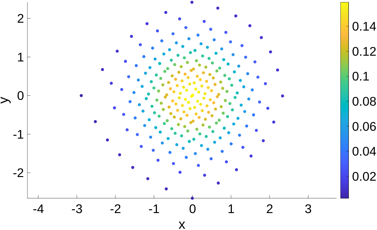
The initial points for the MLS method are sampled from in the following way. First, quasi-random points on the domain are generated using a van der Corput sequence [33]. These points are then mapped to the distribution using the inverse transform sampling method [8]. In Figure 3(a), the initial distribution of points for is plotted. The simulation is performed with an increasing number of particles up to time . The neighborhoods of particles consist of points. Since the characteristic interparticle distance in two dimensions scales as , we refine the maximum time step according to
The eigenvalue-based adaptive criterion does not impose a smaller time step in this test. Because the logarithm of the Gaussian solution remains quadratic, its spatial derivatives are reproduced exactly by the quadratic MLS approximation, up to numerical errors. The observed errors are therefore dominated by the temporal discretization. Accordingly, the Euler and midpoint methods exhibit errors of order and , respectively. The error at final time is measured in the relative norm
| (47) |
The convergence graph for the first-order Euler method and the second-order IMEX midpoint method is shown in Figure 3(b). We observe first- and second-order convergence for the Euler and midpoint methods, respectively, consistent with their temporal discretization errors. In Figure 3(c), the paths of several particles are plotted. As expected, we observe that the particles travel on straight lines outward from the origin.
5.2.2 Stochastic method
We now perform the same test case with the Monte Carlo method described in Section 4.1. One million particles are randomly sampled from the initial distribution. These Monte Carlo particles are then advanced using the discretized SDE for 200 time steps, with , up to time 2. To obtain the osmotic paths, we place several small regions of fixed radius at the same locations as in the MLS simulation, see Figure 3(c). Initially, the small regions contain between 494 and 31,968 particles, depending on the location of the small region compared to the center of the initial distribution. The osmotic paths are then obtained by advancing the location of the small regions using the approximation of the score, see Section 4.2. The locations of the particles and the osmotic paths are plotted in Figure 4(a). As before, we observe the small regions move on radially outward trajectories, with the expected Monte Carlo noise. Initially, some small regions lie at the edge of the particle cloud and therefore contain few particles, resulting in noisy paths. Then, as time evolves, the average number of particles per region decreases, and the same particles spread out over a larger area. Thus, as time increases, the paths also become noisier. In Figure 4(b), the same simulation is performed with the adaptive radius method from Section 4.2.1. Clearly, the adaptive radius selection is able to balance the bias and Monte Carlo error, significantly improving the results.
5.3 Advection-diffusion test case
We now consider a second scenario in which a Gaussian with and is mapped onto a Gaussian at the origin with standard deviation . Due to the difference in means of the distributions, we now also expect advection to take place. In this case, the exact solution is given by a Gaussian with mean and covariance matrix [20]
with . The simulations are performed up to time .
5.3.1 MLS
As in the previous example, we use quasi-randomly distributed points and keep the number of neighbors . The simulation is carried out on grids of progressively finer resolution. Similarly to before, the time step is refined according to
| (48) |
In addition to reporting the error of the density at the final positions (47), we also plot the relative error in the particle positions.
| (49) |
The true final position can be computed by integrating the characteristic equation (12), using the exact solution of the density, with a higher-order Runge-Kutta method. The convergence graph is given in Figure 5. The methods again achieve first-order and second-order for the density and -coordinate. The error in the -coordinate is omitted because it behaves identically to the error in the -coordinate. In Figure 6(a), the initial distribution and final distribution are plotted, as well as several particle paths. We plot both the paths of the particles during simulations, and the paths obtained by integrating the characteristic equation (12) with the exact solution. The midpoint method is also visually more accurate.
5.3.2 Stochastic method
For comparison, we repeat the test case with the Monte Carlo particle method. Ten million Monte Carlo particles are sampled from the initial condition and advanced through time with time step . We place several small regions with initial radius at the same initial locations as in the MLS simulation, see Figure 6(a). Throughout the simulation, the radii are adapted to balance the bias and Monte Carlo error. The results are plotted in Figure 6(b). We observe good agreement between the paths generated by the Monte Carlo method and those computed by integrating the osmotic velocity with an expression for the exact density distribution.
5.4 Transport of a Gaussian across a cylinder
5.4.1 Problem setup
We consider a test case from [18] in which a Gaussian is transported to another Gaussian with a circular obstacle between them. The initial and final distributions are given by
The circular obstacle has radius and is placed at the origin, . The introduction of the obstacle allows us to test how the MLS and Monte Carlo methods handle boundary conditions. Moreover, it provides motivation for using the FPE for point set registration, as solving the FPE on a bounded domain is simpler than addressing optimal transport problems in the presence of obstacles. We perform the simulation with the MLS particle method and the stochastic particle method up to the final time .
5.4.2 MLS
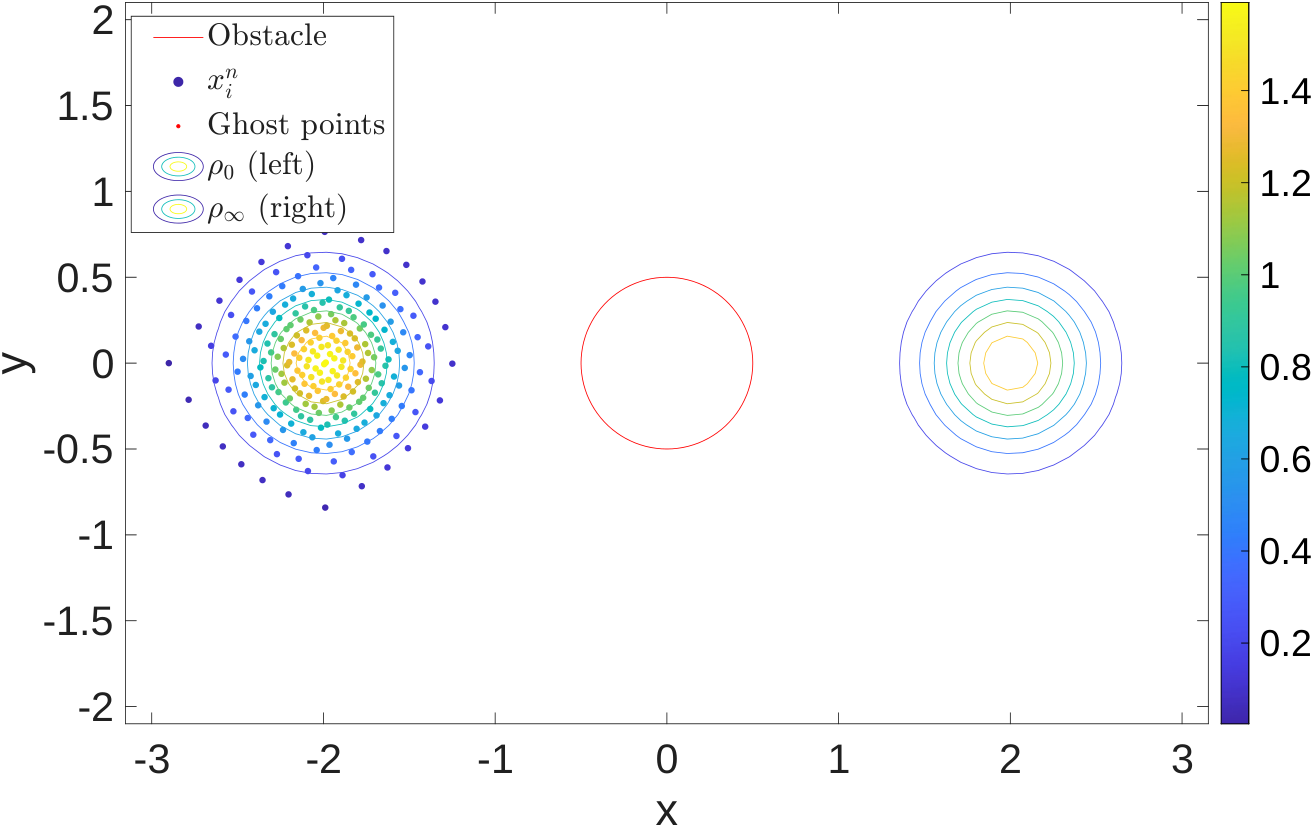
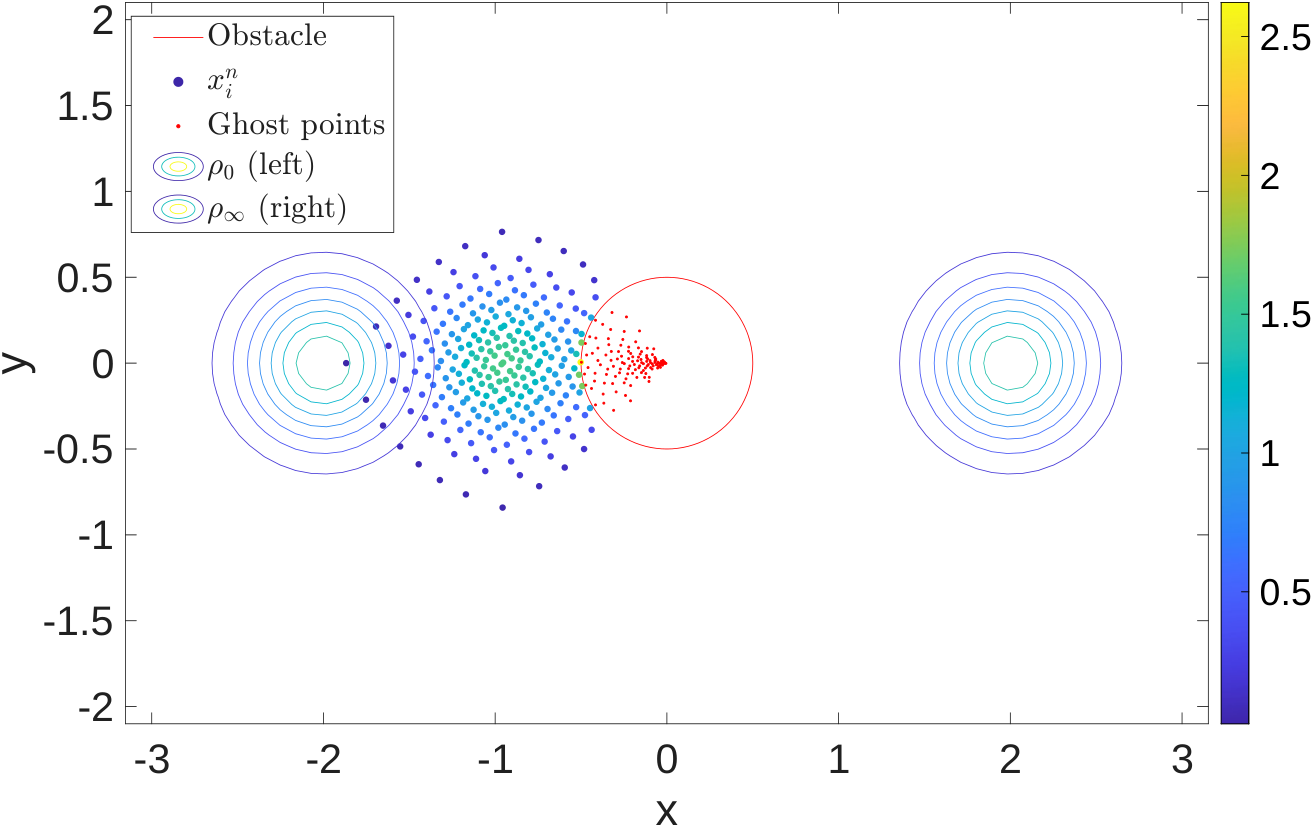
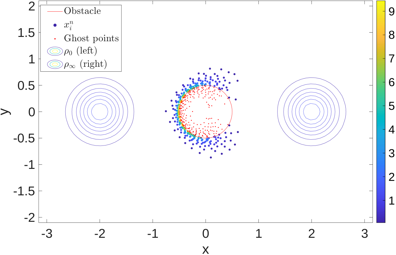
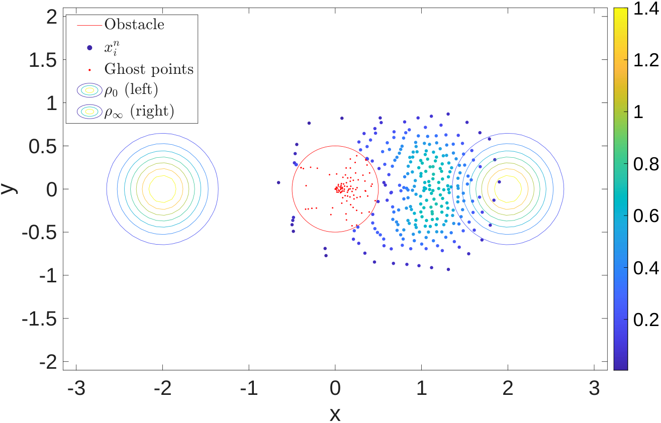
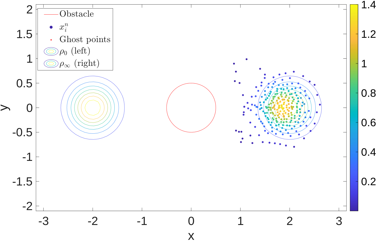
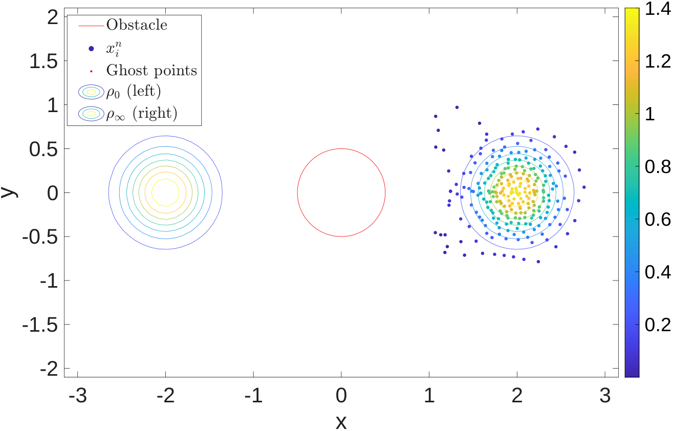
The initial distribution of particles is sampled using quasi-random numbers from the initial distribution . The simulation is performed with time step . We use particles. Each particle is assigned neighbors in every time step. The simulation is performed with the IMEX midpoint method, as it is slightly more accurate than the IMEX Euler method. During the simulation, the adaptive time-stepping criterion reduces the time step when the particle cloud becomes irregular upon interacting with the boundary. The distribution of the particles and the ghost particles at several moments in time are plotted in Figure 7. We observe that the particle distribution splits into two groups, one of which moves along the top of the obstacle, the other along the bottom. As the particle cloud hits the boundary of the obstacle, we observe a significant increase in density. The ghost point method correctly enforces the reflective boundary condition. Behind the obstacle, the groups merge into the final distribution. While the particles were initially distributed according to , at the final time the particle distribution is slightly distorted. We note that the small asymmetries between the upper and lower halves of the distribution are due to the initial asymmetric particle distribution.
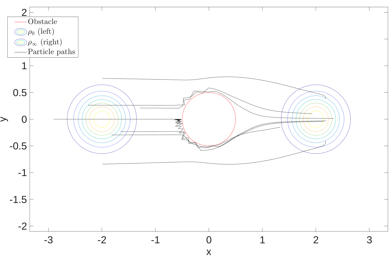
Some particle paths are plotted in Figure 9(a). We observe a flow of particles around the boundary of the obstacle. One particle that approaches the obstacle boundary at a perpendicular angle, somewhat abruptly turns up to avoid the boundary.
5.4.3 Stochastic method
The simulation uses particles. Because steep particle-density gradients develop near the obstacle, we use a relatively small time step of . The radii of the small regions are initialized as and subsequently updated using the adaptive-radius procedure described in Section 4.2.1. Figure 8 shows the Monte Carlo particle distribution at several times. The particle cloud encounters the obstacle, stretches around it, and ultimately detaches from the boundary before converging to the target distribution. The corresponding osmotic paths are shown in Figure 9(b). Near the obstacle, we observe discontinuities in the osmotic paths as the small regions hit the obstacle. This is due to the high density of particles around the obstacle. This very large density gradient, computed through the mean shift vector, briefly overcomes the drift to the target distribution and pushes the small regions back. For some small regions, such as the one that hits the obstacle at a perpendicular angle, this process repeats several times.


5.5 Point set registration across a cylinder
We consider the point set registration problem across a cylinder from [18]. The goal is to map an initial point cloud onto a target point cloud and obtain the trajectories of the mapping. We define the point clouds as
| (50) | ||||
| (51) |
where , , , and . The initial and target point clouds are the left and right halves of a circle separated by a distance of 2. The initial and target point clouds are each approximated using a Gaussian mixture model and kernel density estimation with a Gaussian kernel, see Appendix A. The weights, means and covariance matrices of the GMMs are given in Appendix B. The bandwidths of the initial and target distributions obtained using KDE are . At the origin, we place a cylindrical obstacle with radius .
The two density-estimation techniques yield distinct approximations of the initial and target densities. We apply the midpoint MLS method to both approximations to assess the influence of the density-estimation technique. For a qualitative comparison between the two particle methods under the same density model, we additionally apply the Monte Carlo method using the GMM approximations. All simulations are performed up to the final time .
5.5.1 MLS
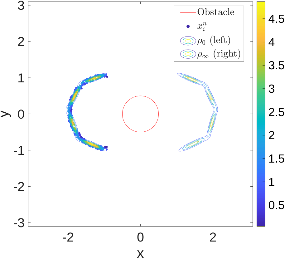
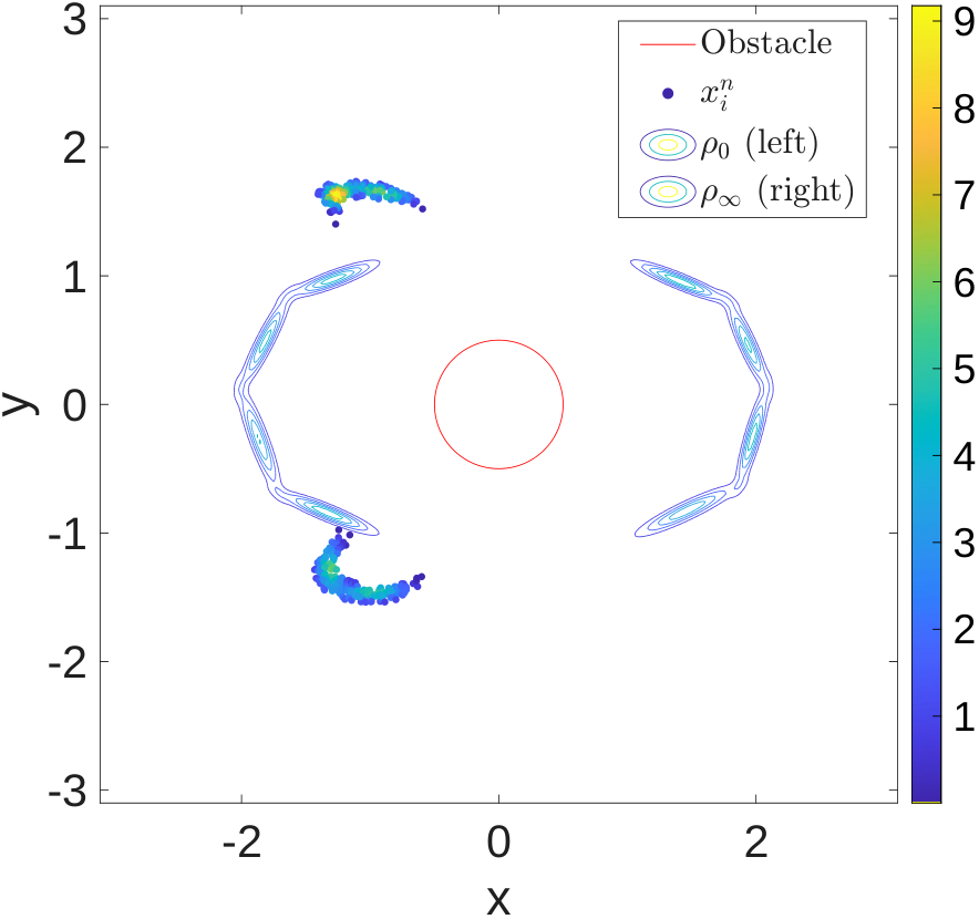
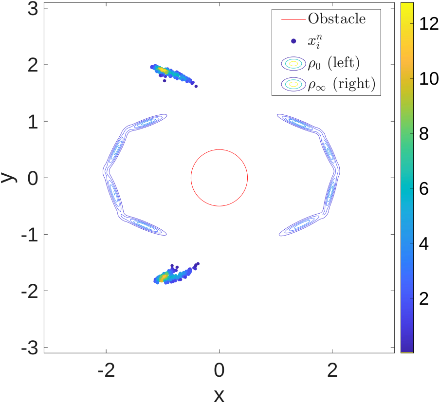
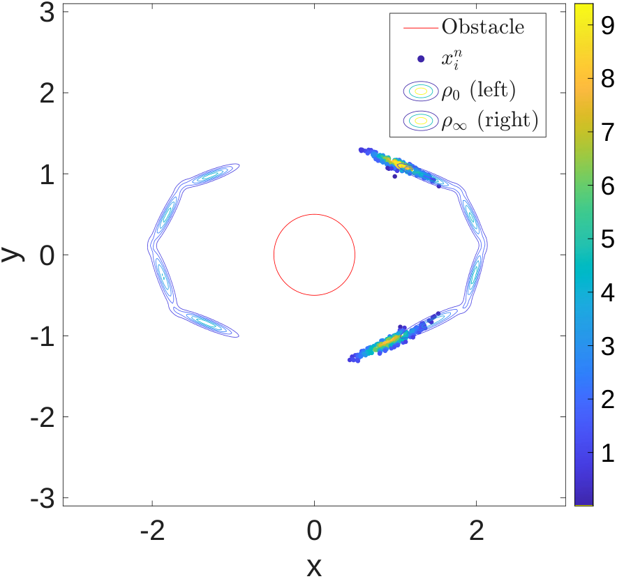
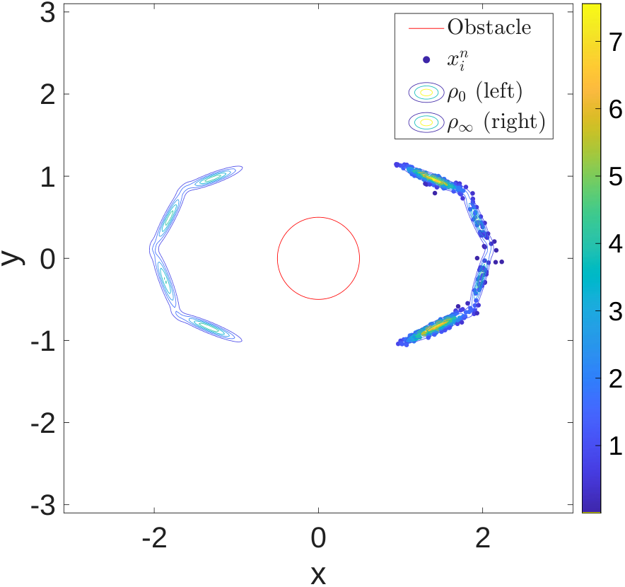
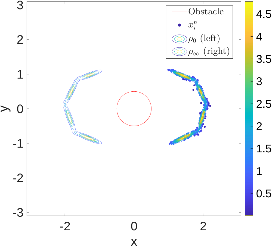
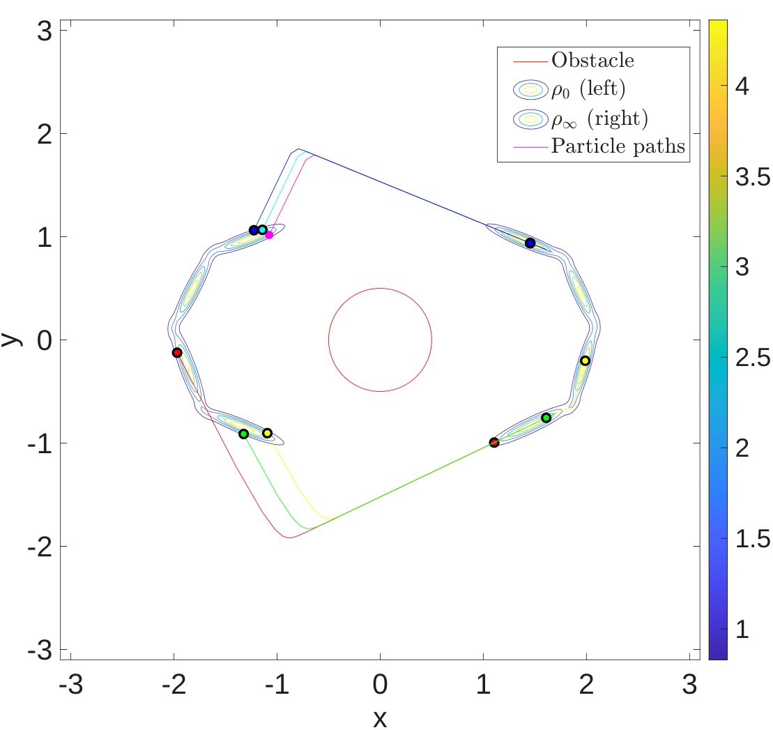
The initial positions of the MLS particles are set to the point cloud given by Equation (50). The MLS particles are thus not ‘evenly’ distributed through the use of the pseudo-random numbers as was the case in the previous simulations. Then, the MLS particles are advanced according to the FPE to the target distribution that is represented by either a GMM or a KDE. We therefore emphasize that the MLS method does not explicitly map the point cloud point-wise to . Instead, the MLS method maps the initial point cloud to the target distribution . It is therefore important for the distribution to fit the target point cloud in the sense that the target point cloud must behave like a sample from . The simulation is conducted with the MLS midpoint method with neighbors and a maximum time step of . We first perform a simulation using a GMM approximation of the target point cloud. The MLS point distribution as well as the initial and target GMMs are plotted in Figure 10 at several time steps. In Figure 10(a), we find that the initial GMM is visually a good approximation for the initial point cloud. Then, we observe that the initial distribution splits into two clouds that advance around the obstacle. We note that the asymmetry in the top and bottom particle clouds is due to the asymmetry of the initial condition. The two particle clouds merge when reaching the final distribution . Note that no ghost points are created during the simulation because the cloud does not move close enough to the obstacle. At the final time, we clearly observe the four Gaussians of the final distribution in the density plot. Some osmotic paths are plotted in Figure 11(a). We find that all particles first move outward and then ‘collapse’ onto the final distribution.
The simulation is repeated using KDE approximations of both the initial and target densities. We emphasize that the initial positions of the MLS particles remain as before. The resulting paths are shown in Figure 11(b). In this case, ghost particles are created and the MLS particles interact with the boundary. We find that the KDE approximation of the initial cloud of points is visibly less accurate than the GMM approximation. In addition, the paths generated from this simulation are qualitatively very different from the GMM case. We conclude that the choice of density estimation procedure has a significant impact on the results if the FPE is used for point set registration.


5.5.2 Stochastic method
We repeat the simulation in which the point clouds are approximated with a GMM. We first sample particles from the GMM that approximates the initial point cloud. We then place six small regions of radius at the initial positions of six selected MLS particles from Equation (50). The simulation is performed with a time step and the adaptive-radius method. The osmotic paths are plotted in Figure 11(c). The paths follow the same qualitative route as those obtained with the MLS method using the GMM, although their final center locations differ appreciably.
5.6 Discussion
For the purpose of point set registration, the two particle methods for the FPE presented here are viable options. The MLS method, although the more difficult of the two to implement, yields accurate results. Thanks to the use of an adaptive stencil, the method can handle test cases in which the point cloud undergoes strong expansion (Section 5.3) and deformation (Section 5.4). In addition, the ghost point method correctly enforces reflective boundary conditions, which enables point set registration in bounded domains. We do note that stability of meshfree methods remains an open question. There is no guarantee of the stability of meshfree discretizations for every possible point cloud. Hence, adaptive time stepping criteria such as the one presented in Section 3.2.1 remain necessary. Contrary to meshfree methods, the stability of Monte Carlo methods for SDEs is well-understood. Moreover, the Monte Carlo method is effectively trivial to implement and very easily parallelizable, yielding potentially very efficient algorithms for point set registration. For the purpose of tracing the osmotic paths, the Monte Carlo method inherently introduces noise to the mapping of the point clouds. However, the results in Section 5.2 demonstrate that the adaptive radius method substantially reduces this effect. Finally, we note that in regions with large density variations, the current mean-shift approach to estimate the score (Section 5.4) is sensitive to the time step and size of the region.
6 Conclusion and Outlook
In this work, we propose two particle-based methods for point set registration in bounded domains, both grounded in the Fokker-Planck formulation of probability transport. By recasting the registration problem as the evolution of a probability density toward a prescribed target distribution, we obtain a continuous flow of mappings that naturally respects mass conservation and boundary constraints while avoiding explicit point-to-point matching.
The first method is a deterministic particle approach based on a moving least squares discretization of the S-formulation of the Fokker-Planck equation. By evolving particles according to the drift induced by the target distribution and resolving diffusion on a dynamically deforming particle cloud, this method directly produces coherent transport paths suitable for registration. A key feature of this approach is the use of a ghost point technique to impose reflective boundary conditions, which enables a consistent and robust treatment of walls and obstacles without the need for mesh generation or domain truncation. The numerical experiments demonstrate that the method can accurately capture strong compression, expansion, and splitting of particle clouds induced by both the drift and the domain geometry.
The second method adopts a stochastic viewpoint and relies on Monte Carlo simulation of the reflected Langevin dynamics associated with the Fokker-Planck equation. Rather than solving the PDE explicitly, this approach evolves large ensembles of particles and reconstructs macroscopic osmotic paths from the stochastic trajectories using a local approximation of the score of the evolving particle distribution. While inherently noisy, this method is straightforward to implement, embarrassingly parallel, and highly scalable, making it particularly attractive for high-dimensional settings where deterministic discretizations become prohibitively expensive. The numerical results highlight that the two approaches are complementary. The MLS-based method offers higher accuracy and smoother trajectories at a relatively modest particle count, at the cost of additional algorithmic complexity and stability considerations. In contrast, the Monte Carlo method trades deterministic accuracy for simplicity and scalability and provides a viable alternative when large numbers of particles and parallel computing resources are available.
Several directions for future work naturally arise. On the deterministic side, adaptive strategies for stencil selection, time stepping, and particle refinement could further improve robustness in regions of strong deformation or near boundaries. On the stochastic side, an adaptive time-stepping procedure could enhance the quality of the recovered osmotic paths. In view of developing a practically viable point set registration method, a systematic investigation of different density estimation techniques and their influence on transport paths would also be of significant interest. Finally, an interesting direction for future research is the study of the Schrödinger bridge problem in bounded domains [9].
Acknowledgments: This work was supported by the European Union’s Framework Program for Research and Innovation Horizon Europe under the Marie Skłodowska-Curie Doctoral Networks action (HORIZON-MSCA-2021-DN-01), Grant Agreement No. 101072546 (DATAHYKING).
Appendix A Density estimation
The first step of our method consists of estimating the densities and that enter (2). The broad literature on density estimation ranges from classical statistical methods [14] to recent methods closely linked to generative artificial intelligence [28]. The choice of method critically depends on the number of data points, the dimension , and the task of interest. In this work, we target two- and three-dimensional domains and expect datasets of moderate size, . Therefore, in the numerical experiments, we consider two methods: kernel density estimation (KDE) and Gaussian mixture models (GMMs).
A.1 Kernel density estimation
We introduce the kernel that satisfies
| (52a) | |||
| Next, given the samples , , we define the KDE: | |||
| (52b) | |||
| Here, denotes the surface measure of the unit sphere in , is the kernel bandwidth, and is chosen so that . If , then . In a bounded domain, the normalization constant generally also depends on the sample locations because the kernels are truncated by the boundary. | |||
For sufficiently smooth densities, the estimator converges in probability to the true density under the standard conditions and as . The asymptotically optimal bandwidth scales as [45]. In practice, we use cross-validation to determine . We consider leave-one-out cross-validation (LOOCV) [40] and least-squares cross-validation (LSCV) [45, Chapter 6.1], which lead to similar results in the experiments of Section 5.
The choice of the kernel function is important for both approximation and stability. The kernel should be sufficiently regular to ensure that its gradient is Lipschitz continuous and should be strictly positive within its support. Its tail behavior also plays a major role in the numerical approximation of the FPE. For rapidly decaying kernels, if a unique closest sample dominates the sum in the far field, then (52b) can be approximated by
which implies
and thus
| (53) |
Table 1 reports the expression of for widely used kernels. We observe markedly different behaviors of in the far field.
| Kernel | ||
|---|---|---|
| Gaussian | ||
| Matérn () | ||
| inverse multiquadric |
For Gaussian kernels (), we find : this implies that the advection term of the FPE satisfies
| (54) |
in the far field; on the other hand, for inverse multiquadric kernels ( with ), we find . Although the nearest-sample approximation need not hold for this heavy-tailed kernel, a direct expansion of the full KDE shows that its score vanishes in the far field. We leave a detailed comparison of kernel functions and their impact on point set registration to future work.
A.2 Gaussian mixture models
GMMs are widely used for density estimation in low dimensions. They provide a compact representation of a density in terms of multivariate Gaussian components,
| (55) |
where the weights satisfy , the means satisfy , and the covariance matrices satisfy , where denotes the set of symmetric positive definite matrices. As in [17], we use the MATLAB function fitgmdist to fit the GMMs and the Akaike information criterion (AIC) [14, Chapter 7] to select . To improve numerical robustness, we set the RegularizationValue option of fitgmdist to .
Appendix B GMM parameters
In Section 5.5, the initial and target distributions are each approximated by a GMM. The weights, means, and covariance matrices of each component are listed below. All reported values are rounded to four decimal places; the simulations use the full-precision parameters provided in the accompanying code [46]. Consequently, the displayed mixture weights may not sum exactly to one and should be renormalized if used directly.
B.1 Initial distribution
Weights: .
Means:
Covariances:
B.2 Target distribution
Weights: .
Means:
Covariances:
References
- [1] (2017) Lecture notes on the DiPerna–Lions theory in abstract measure spaces. In Annales de la Faculté des sciences de Toulouse: Mathématiques, Vol. 26, pp. 729–766. Cited by: §2.1.
- [2] (1995) Implicit-Explicit Methods for Time-Dependent Partial Differential Equations. SIAM Journal on Numerical Analysis 32 (3), pp. 797–823 (en). External Links: ISSN 0036-1429, 1095-7170, Link, Document Cited by: §3.2.2.
- [3] (2019) Voxelmorph: a learning framework for deformable medical image registration. IEEE transactions on medical imaging 38 (8), pp. 1788–1800. Cited by: §1.1.
- [4] (2005) Computing large deformation metric mappings via geodesic flows of diffeomorphisms. International journal of computer vision 61, pp. 139–157. Cited by: §1.1.
- [5] (2023) Feature-based image metamorphosis. In Seminal Graphics Papers: Pushing the Boundaries, Volume 2, pp. 529–536. Cited by: §1.1.
- [6] (2015) Local and global estimates of solutions of hamilton–jacobi parabolic equation with absorption. Advances in Differential Equations 20 (11–12), pp. 1077–1114. Cited by: §2.2.
- [7] (2021) Accurately computing the log-sum-exp and softmax functions. IMA Journal of Numerical Analysis 41 (4), pp. 2311–2330 (en). External Links: ISSN 0272-4979, 1464-3642, Link, Document Cited by: §3.4.
- [8] (1998) Monte Carlo and quasi-Monte Carlo methods. Acta Numerica 7, pp. 1–49 (en). External Links: ISSN 0962-4929, 1474-0508, Link, Document Cited by: §1.2, §5.2.1.
- [9] (2021) Reflected Schrödinger bridge: density control with path constraints. In 2021 American Control Conference (ACC), pp. 1137–1142. External Links: Document Cited by: §6.
- [10] (2024) Stencil and kernel optimisation for mesh-free very high-order generalised finite difference method. Mathematics and Computers in Simulation 218, pp. 49–78 (en). External Links: ISSN 03784754, Link, Document Cited by: §1.2.
- [11] (2024) Model order reduction by convex displacement interpolation. Journal of Computational Physics 514, pp. 113230 (en). External Links: ISSN 00219991, Link, Document Cited by: §1.2.
- [12] (2025) Improving the robustness of neural ODEs with minimal weight perturbation. arXiv preprint arXiv:2501.10740. Cited by: Remark A.1.
- [13] (1975) The estimation of the gradient of a density function, with applications in pattern recognition. IEEE Transactions on Information Theory 21 (1), pp. 32–40. External Links: ISSN 0018-9448, 1557-9654, Link, Document Cited by: §4.2.
- [14] (2009) The elements of statistical learning. Springer Series in Statistics, Springer New York Inc., New York, NY, USA. Cited by: §A.2, Appendix A, §3.4.
- [15] (2014) Advection modes by optimal mass transfer. Physical Review E 89 (2), pp. 022923. Cited by: §1.1.
- [16] (2022) Mapping of coherent structures in parameterized flows by learning optimal transportation with Gaussian models. Journal of Computational Physics 471, pp. 111671. Cited by: §1.1.
- [17] (2025) Point-set registration in bounded domains via the Fokker–Planck equation. Comptes Rendus. Mathématique 363 (G8), pp. 809–824. Cited by: §A.2, §1.1, §1.1, §1.2, §2.1, §2.1.
- [18] (2025) Point-set registration in bounded domains via the Fokker–Planck equation. Comptes Rendus. Mathématique 363 (G8), pp. 809–824 (en). External Links: ISSN 1631-073X, 1778-3569, Link, Document Cited by: §5.4.1, §5.5, §5.
- [19] (2020) An enhanced weakly-compressible MPS method for free-surface flows. Computer Methods in Applied Mechanics and Engineering 360, pp. 112771 (en). External Links: ISSN 00457825, Link, Document Cited by: §1.2.
- [20] (2007) Stochastic processes in physics and chemistry. 3rd ed edition, North-Holland personal library, Elsevier, Amsterdam, The Netherlands Oxford, UK (eng). External Links: ISBN 978-0-444-52965-7 Cited by: §5.3.
- [21] (1998) Brownian Motion and Stochastic Calculus. Graduate Texts in Mathematics, Vol. 113, Springer New York, New York, NY (en). External Links: ISBN 978-0-387-97655-6 978-1-4612-0949-2, Link, Document Cited by: §1.2.
- [22] (2020) High order difference schemes using the local anisotropic basis function method. Journal of Computational Physics 415, pp. 109549 (en). External Links: ISSN 00219991, Link, Document Cited by: Remark 3.1.
- [23] (2022) High-order simulations of isothermal flows using the local anisotropic basis function method (LABFM). Journal of Computational Physics 449, pp. 110760 (en). External Links: ISSN 00219991, Link, Document Cited by: Remark 3.1.
- [24] (1992) Numerical Solution of Stochastic Differential Equations. Springer Berlin Heidelberg, Berlin, Heidelberg. External Links: ISBN 978-3-642-08107-1 978-3-662-12616-5, Link, Document Cited by: §4.1, §4.1.
- [25] (1998) Numerical analysis of breaking waves using the moving particle semi-implicit method. International Journal for Numerical Methods in Fluids 26 (7), pp. 751–769 (en). External Links: ISSN 0271-2091, 1097-0363, Link, Document Cited by: §1.2.
- [26] (2001) Grid free method for solving the poisson equation. Technical report Technical Report 25, Fraunhofer-Gesellschaft. External Links: Link Cited by: §1.2.
- [27] (2026) Parametric vector flows for registration fields in bounded domains with applications to nonlinear interpolation of shock-dominated flows. arXiv preprint arXiv:2601.22712. Cited by: §1.1.
- [28] (2025) The principles of diffusion models. arXiv preprint arXiv:2510.21890. Cited by: Appendix A.
- [29] (1981) Surfaces generated by moving least squares methods. Mathematics of Computation 37 (155), pp. 141–158 (en). External Links: ISSN 0025-5718, 1088-6842, Link, Document Cited by: §1.2.
- [30] (1998) The approximation power of moving least-squares. Mathematics of Computation 67 (224), pp. 1517–1531 (en). External Links: ISSN 0025-5718, 1088-6842, Link, Document Cited by: §1.2.
- [31] (1984) Stochastic differential equations with reflecting boundary conditions. Communications on Pure and Applied Mathematics 37 (4), pp. 511–537. Cited by: §2.3, §4.1.
- [32] (2010) Point set registration: coherent point drift. IEEE transactions on pattern analysis and machine intelligence 32 (12), pp. 2262–2275. Cited by: §1.1.
- [33] (1992) Random number generation and quasi- Monte Carlo methods. Regional conference series in applied mathematics, Society for Industrial and Applied Mathematics, Philadelphia, Pa (eng). External Links: ISBN 978-0-89871-295-7 Cited by: §5.2.1.
- [34] (2014) Stochastic processes and applications. Springer. Cited by: §2.3.
- [35] (2025) Registration-based nonlinear model reduction of parametrized aerodynamics problems with applications to transonic Euler and RANS flows. Journal of Computational Physics 521, pp. 113576. Cited by: §1.1.
- [36] (1990) A particle method for collisional kinetic equations. I. Basic theory and one-dimensional results. Journal of Computational Physics 87 (2), pp. 270–300. Cited by: Remark 2.1.
- [37] (1990) Deterministic diffusion of particles. Communications on Pure and Applied Mathematics 43 (6), pp. 697–733. Cited by: Remark 2.1.
- [38] (2006) M-matrices in meshless finite difference methods. Berichte aus der Mathematik, Shaker, Aachen (eng). External Links: ISBN 978-3-8322-5643-2 Cited by: §3.1, §3.1.
- [39] (2020) Score-Based Generative Modeling through Stochastic Differential Equations. arXiv. Note: Version Number: 2 External Links: Link, Document Cited by: §1.2.
- [40] (1974) Cross-validatory choice and assessment of statistical predictions. Journal of the royal statistical society: Series B (Methodological) 36 (2), pp. 111–133. Cited by: §A.1.
- [41] (2018) Conservation and accuracy in meshfree generalized finite difference methods. Fraunhofer Verlag, Stuttgart (eng). External Links: ISBN 978-3-8396-1325-2 Cited by: Remark 3.2.
- [42] (2020) A registration method for model order reduction: data compression and geometry reduction. SIAM Journal on Scientific Computing 42 (2), pp. A997–A1027. Cited by: §1.1.
- [43] (2014) Least squares moving particle semi-implicit method. Computational Particle Mechanics 1 (3), pp. 277–305 (en). External Links: ISSN 21964386, Link, Document Cited by: §1.2.
- [44] (2023) Compact moving particle semi-implicit method for incompressible free-surface flow. Computer Methods in Applied Mechanics and Engineering 414, pp. 116168 (en). External Links: ISSN 00457825, Link, Document Cited by: §1.2.
- [45] (2006) All of nonparametric statistics. Springer. Cited by: §A.1.
- [46] Moving Least Squares Method for Point Set Registration Cited by: Appendix B, §5.
- [47] (2015) Location and scale mixtures of Gaussians with flexible tail behaviour: properties, inference and application to multivariate clustering. Computational Statistics & Data Analysis 90, pp. 61–73. Cited by: Remark A.1.
- [48] (1995) Mean shift, mode seeking, and clustering. IEEE Transactions on Pattern Analysis and Machine Intelligence 17 (8), pp. 790–799 (en). External Links: ISSN 01628828, Link, Document Cited by: §4.2.
- [49] (2019) A review of point set registration: from pairwise registration to groupwise registration. Sensors 19 (5), pp. 1191. Cited by: §1.1.
- [50] (2003) Stochastic differential equations. 6th edition, Springer. Cited by: §2.3.