Before It Fades: Reinforcing Temporal Representations at Inference Time in VideoLLMs
Abstract
Video Large Language Models (VideoLLMs) receive frames in sequential order and interpret how visual content evolves along the temporal axis, yet temporal reasoning remains a persistent weakness across architectures. Reversing the frame order of a video, a transformation that should invert temporal answers, often leaves the final prediction unchanged. We investigate where this failure originates by defining the temporal divergence vector , the layer-wise representational difference induced by reversing temporal order. Tracking its magnitude across layers reveals a consistent temporal divergence profile where the divergence peaks at intermediate layers and progressively diminishes toward the output. We confirm this peak is specific to temporal reasoning and functionally critical for predictions, establishing that VideoLLMs acquire temporal information at intermediate layers but fail to maintain it to the output. This progressive fading motivates our method, Temporal Activation Injection (TAI), which extracts at the peak of the profile for each input and reinjects it into subsequent layers following the measured decay. TAI requires no training and consistently improves temporal reasoning across three VideoLLMs and four benchmarks with negligible impact on non-temporal tasks. Code is available at https://github.com/Youngwoo-git/Before-It-Fades.
1 Introduction
Video Large Language Models (VideoLLMs) enable interpreting ordered sequences of visual frames through the reasoning capabilities of large language models, advancing video understanding across tasks [2, 1, 3]. Temporal reasoning is central to this process, as these models receive frames in sequential order and interpret how visual content evolves along the temporal axis. Yet it remains a persistent weakness across architectures [4, 16, 26], and Fig. 1 illustrates a representative failure case. Reversing the frame order of a video is a transformation that should invert the answer to a temporal question, yet the model produces the same prediction for both inputs, failing to perform temporal reasoning.
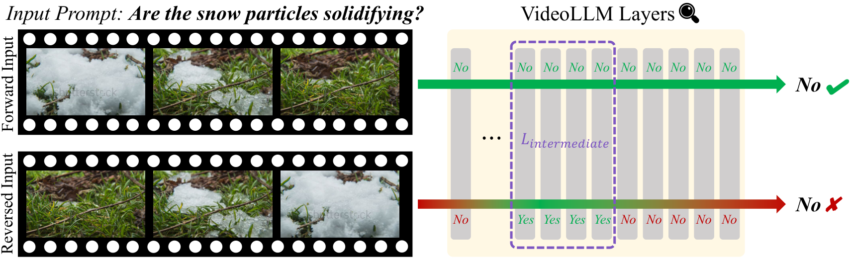
Improving temporal reasoning in VideoLLMs has been approached from multiple directions. Training-based methods learn temporal capabilities through dedicated objectives [26, 14]. Inference-time methods, predominantly contrastive decoding [28, 18, 25], contrast output distributions from temporally distorted inputs to adjust final predictions. Both regard temporal reasoning failure as a given limitation and address it externally, without investigating where it originates. However, we observe in Fig. 1 that this failure may not be inherent, as the representation at assigns a higher probability to the correct answer for the reversed input before subsequent layers overturn it. This indicates that representations sensitive to temporal order emerge but are not maintained through the remaining layers, raising our central question: where do representations sensitive to temporal order concentrate and shift across layers, and how can we intervene there to improve temporal reasoning?
To answer this question, we quantify how these representations change across layers, identifying where they concentrate and how they evolve toward the output. To isolate the contribution of temporal order in these representations, we reverse the frame order of each video to construct a pair that differs only along the temporal axis while sharing all spatial content and text conditioning. To measure this contribution at each layer, we define the representational difference between the two inputs as the temporal divergence vector . Tracking its normalized magnitude across layers produces the temporal divergence profile, which follows a shared pattern across all architectures we evaluate: the divergence peaks in the mid-to-late layers, then progressively diminishes toward the output. We confirm that this peak is specific to temporal reasoning through question-conditioned analysis and that it is functionally critical for the model’s predictions through causal intervention. These results establish that VideoLLMs acquire temporal information at intermediate layers and rely on it for their predictions, yet this information progressively fades before reaching the output.
This progressive fading presents a natural intervention point, motivating our method, Temporal Activation Injection (TAI), which extracts at the peak of the temporal divergence profile for each input and reinjects it into subsequent layers following the measured decay. captures the direction and magnitude by which temporal information is expressed in the representation at each layer, and adding it to subsequent layers compensates for the signal that the model produces but fails to maintain. TAI uses the temporal divergence profile itself as layer-wise weights, grounding the intervention in quantities measured from the model. TAI requires no training, adapts to each input through its own , and operates entirely at inference time without modifying model weights.
We evaluate TAI across three VideoLLMs with diverse architectures [2, 1, 3] on temporal reasoning benchmarks [16, 4, 26] and a general video understanding benchmark [13]. TAI consistently improves temporal reasoning across all three models with negligible impact on non-temporal performance. Improvements concentrate on categories whose answers depend on frame order, while categories invariant under reversal receive minimal effect, confirming that TAI selectively targets temporal reasoning. Across all experiments, the temporal divergence profile serves as both an analytical tool that reveals where temporal information concentrates and a practical basis for targeted intervention.
Our contributions are as follows:
- •
We introduce the temporal divergence vector and its layer-wise profile, revealing that VideoLLMs acquire temporal information at intermediate layers but fail to maintain it to the output.
- •
We propose Temporal Activation Injection (TAI), a training-free method that leverages the temporal divergence profile to improve temporal reasoning in VideoLLMs.
- •
We demonstrate consistent improvements in temporal reasoning across three VideoLLMs and four benchmarks with negligible impact on non-temporal tasks.
2 Related Works
2.1 Temporal Reasoning in VideoLLMs
VideoLLMs [2, 1, 3, 10, 15, 29] integrate video encoders [30, 24] with LLM backbones and adopt temporal-aware enhancements [21, 19], yet consistently struggle with temporal reasoning [4, 16]. Prior work has approached this limitation from multiple angles. Through probing and training, T3 [14] demonstrates that video embeddings capture sufficient temporal information yet the LLM decoder fails to leverage it, localizing the bottleneck to the language model without identifying where within it the deficiency arises. ArrowRL [26] observes that models show little sensitivity at the output level when videos are reversed or shuffled, and addresses it through reinforcement learning. Mechanistic analyses offer a complementary perspective. Kim et al. [7] find that temporal reasoning relies on a sparse set of effective pathways rather than the full attention graph, and causal interventions on the last token confirm that temporal information is progressively aggregated into the prediction position through cross-modal attention [21]. However, these analyses trace how temporal information flows but not how this signal evolves in subsequent layers. Our work builds on these findings, establishing that the temporal signal peaks at intermediate layers and progressively diminishes toward the output, and addresses this decay without additional training.
2.2 Inference-Time Model Steering
Recent methods steer LLM behavior at inference time by manipulating either intermediate hidden states or output distributions, and several have been adapted to improve temporal faithfulness in VideoLLMs. In the first direction, Representation Engineering (RepE) [31] controls model behavior by manipulating concept directions within hidden states without modifying model weights. ITI [12] trains linear probes per attention head to locate truthful directions, and CAA [20] computes mean activation differences from contrastive pairs. SADI [23] and CAST [9] adapt the intervention to input context but still rely on labeled data to learn the steering directions. Rather than steering hidden states, a separate line of work targets temporal faithfulness through contrastive decoding. TCD [28], VTD [18], and SEASON [25] contrast output distributions from temporally distorted inputs to suppress unfaithful predictions, while DINO-HEAL [11] adjusts predictions using features from a separate vision model. These methods operate without examining the model’s internal representations, intervening at the output level or relying on external signals. Our analysis reveals that temporal signals peak at intermediate layers and substantially degrade by the time logits are produced. Our method operates at the intermediate representation level, extracting input-specific temporal vectors where temporal information concentrates without ground-truth annotations or parameter updates.
3 Analysis of Temporal Representations
Reversing the temporal order of frames alters the internal representations of models during inference, but where and how much the activations diverge across layers has not been characterized. We term this layer-wise activation divergence the temporal divergence. Since the reversed video shares identical spatial content and text conditioning with the original, any difference in hidden states isolates the contribution of temporal order. We pair each input video with its time-reversed counterpart , obtained by reversing the frame sequence along the temporal axis. We conduct our analysis across three VideoLLMs of comparable scale with diverse architectures: Qwen2.5-VL-7B [2], Qwen3-VL-8B [1], and InternVL2.5-8B [3]. We use 50 temporally reversed video pairs with binary temporal questions from TempCompass [16], where ground-truth answers invert under reversal.

3.1 Layer-wise Temporal Divergence
To track temporal divergence across layers, we focus on the last token, which under causal attention is the only position that has attended to all preceding visual and textual tokens [31, 12]. We extract the hidden state at this position for each layer , where is the number of layers and the hidden dimension. We denote the last token hidden states under the two inputs as and , and define the temporal divergence vector . The magnitude of at a given layer reflects how much the hidden state changes when frame order is reversed. For fair comparison across layers, we normalize by the forward activation norm to account for the monotonic growth of hidden state magnitudes with layer depth, yielding the scalar normalized temporal divergence :
| (1) |
We compute for each of the three models and report the mean temporal divergence profiles in Fig. 2 (a, solid) using temporal questions from TempCompass [16]. A consistent pattern emerges across all architectures. Through the initial layers, remains low as the model processes visual and textual tokens without substantial divergence. Starting from the intermediate layers, rises sharply and peaks in the mid-to-late layers. After this peak, progressively declines toward the final layers, falling to values comparable to or below those at the start, though some models exhibit a slight uptick near the last layer consistent with hidden state jumps [22]. The convergence of this profile across models with different vision encoders, LLM backbones, positional encoding schemes, and training recipes indicates that captures a shared computational regularity in how decoder-only VideoLLMs process frame order dependent information.
This convergence across architectures reflects more than the flow of temporal information through the model, as quantifies where temporal information concentrates at the representation level across layers. Reversing the frame sequence inverts the answer to temporal questions while keeping the prompt and all other input components intact, so any divergence in the resulting representations isolates the effect of altering the temporal axis. By tracking this divergence at the last token, the position whose representation drives the final prediction, captures how temporal information reaches the prediction across layers. Because is computed only with hidden states from a single forward pass on each video, it requires no ground-truth annotations, trained probes, or model modification, and can be applied to characterize any VideoLLM that exposes intermediate representations.
3.2 Temporal Specificity of Divergence
has favorable properties as a diagnostic for finding the place of divergence, yet whether the divergence at the peak is bound to temporal reasoning specifically remains to be verified. The peak in may capture every representational difference caused by reversal, or it may reflect the subset specific to temporal reasoning. To examine which of these holds, we hold the video pair constant and vary only the question. If the divergence at the peak is determined by the video alone, should remain stable across different questions on the same video pair. If instead responds to what the model is asked to reason about, the profile should shift with the question. We test this by evaluating on the same forward and reversed video pairs under three question conditions. (1) Temporal questions from TempCompass [16] that require frame order awareness to answer (e.g., Is the person moving downwards?), and two control conditions we construct to isolate temporal specificity: (2) a spatial question whose answer does not change under reversal (Is this video filmed indoors or outdoors?), and (3) a video-irrelevant question unrelated to visual content (Does a week have seven days?).
Fig. 2 (a, dashed and dotted) illustrates under the two non-temporal conditions on the same video pairs. Unlike the temporal condition described in Sec. 3.1, the distinctive peak is substantially attenuated and remains comparatively low through the later layers. The same video pairs produce different profiles depending solely on the question, confirming that the peak reflects the last token selectively aggregating temporal information when the task demands it rather than passively inheriting frame order differences from the visual input. The peak in therefore provides a reliable, question-conditioned indicator of where to intervene for temporal reasoning.
3.3 Functional Importance and Signal Decay
The peak in emerges where the last token selectively aggregates temporal information, but whether the model actually depends on this signal for its predictions remains to be tested. To assess this, we apply attention knockout [5] to the last token at each layer, setting the attention mask for the last token position attending to all positions at layer . This removes the last token’s access to the video and prompt tokens it would normally attend to, blocking the flow of information into the prediction position at that layer. We sweep this intervention across all layers and measure the resulting change in ground truth answer probability on subtasks related to temporal reasoning [16]. Fig. 2 (b) shows that blocking layers in the early or final stages produces modest effects, while blocking the region around the peak causes the largest probability drop. This region aligns precisely with the peak in Fig. 2 (a), confirming that the temporal information concentrated at these layers is actively utilized for the final prediction rather than an incidental activation pattern. The same layers that produce the largest temporal divergence in Sec. 3.1 and respond selectively to temporal questions in Sec. 3.2 are also where the last token draws most heavily on temporal information for its prediction.
The profiles in Fig. 2 (a) further reveal that this temporal information does not persist beyond the peak. After the peak, declines progressively across all three models, consistent with broader findings that later LLM layers contribute diminishing semantic value [6]. This decay at the representation level accounts for the prediction-level failure observed in Fig. 1, where the correct answer at is overturned by subsequent layers. The profile therefore identifies both where to secure the temporal information before it fades and how much compensation each subsequent layer requires, presenting a natural intervention point grounded in the temporal divergence profile of the model. The experiments in Sec. 5 validate that compensating for this decay consistently improves temporal reasoning across all models, with the specificity analysis in Sec. 5.3 confirming that the compensation selectively targets temporal categories of the benchmarks with minimal effect on non-temporal ones, suggesting the decay constitutes an addressable stage of inference for temporal reasoning.
4 Temporal Activation Injection

The natural intervention point identified in Sec. 3, where temporal information concentrates and subsequently diminishes, motivates our method, Temporal Activation Injection (TAI), illustrated in Fig. 3. TAI extracts temporal information at the peak of the profile and reinjects it into the last token at subsequent layers where this information diminishes, compensating for the decay identified in Sec. 3.3. The entire process operates on hidden states that the model already computes during inference, requiring no ground-truth annotations, additional training, or model modification.
Extraction. Given an input video and prompt , we construct its time-reversed counterpart by reversing the frame sequence. The analysis in Sec. 3 identified that temporal information concentrates around the peak layers of the profile and progressively decays afterward. We therefore set the source layer to the peak immediately before this decay begins and process through the model up to , capturing the last token hidden state . All layers beyond are bypassed via early termination to avoid unnecessary computation. We then process through the full model, capturing at the same layer and applying injection at subsequent layers as described below.
| (2) |
We do not normalize to utilize the full directional vector in the representation space. While the profile-derived weights distribute the injection across layers at the model level, the magnitude of adapts the injection strength at the input level, so that videos sensitive to frame reversal naturally receive stronger injection while temporally invariant inputs receive near-zero correction. Unlike fixed steering vectors, is extracted separately for each video and remains input-specific.
Profile-guided injection. The profile measured in Sec. 3.1 demonstrates that the temporal divergence concentrates around the peak layer and progressively decreases in the subsequent layers. We leverage this empirically measured profile directly as a per-layer injection schedule. For each layer , we modify the last token hidden state as:
| (3) |
where is a global scaling coefficient and is pre-computed per model from the mean profile, while adapts per input. Because follows the profile rather than a uniform or heuristic schedule, the injection is grounded in quantities measured from the model. Post-peak layers whose representations still carry a substantial temporal component receive proportionally larger injection, while deeper layers receive lighter additions that respect their established role in shaping the final prediction [6, 5]. Since the profile is measured at the last token position, injection is applied exclusively at that position, leaving all other token representations and model parameters unchanged.
Implementation Details. The source layer is set to the peak of the profile before the decay begins, which consistently falls in the mid-to-late layers across the models we evaluate. The profile weights are pre-computed once per model from 50 forward-reverse video pairs with temporal questions from TempCompass [16], requiring only the videos and questions without any ground-truth annotations, and stored as a lightweight configuration. Since the profile captures a structural property of the model rather than properties of specific videos, it generalizes across inputs and stabilizes with relatively few samples, as detailed in Appendix B.
5 Experiments
5.1 Experimental Setup
We apply TAI to three VideoLLMs of comparable scale with diverse architectures: Qwen2.5-VL-7B, Qwen3-VL-8B, and InternVL2.5-8B. For temporal reasoning, we evaluate on TempCompass [16], TVBench [4], and AoTBench [26]. For general video understanding, we use MVBench [13]. We compare against recent training-free methods TCD [28] and DINO-HEAL [11], and the training-based ArrowRL [26]. All experiments are conducted on a single A6000 GPU with 16-frame uniform temporal sampling, and accuracy is reported in %. The divergence profile required for profile-guided injection is computed once per model in Sec. 3 and reused across all evaluations. The scaling coefficient in Eq. 3 is set per model and held constant across all benchmarks for that model.
| Models | Training- free | TempCompass | TVBench | ||||||||||||||
|---|---|---|---|---|---|---|---|---|---|---|---|---|---|---|---|---|---|
| Act | Attr | Dir | Ord | Spd | AVG | AC | AL | AS | ES | MD | OC | OS | ST | UA | AVG | ||
| Qwen2.5-VL-7B | - | 94.9 | 77.2 | 59.1 | 75.8 | 59.2 | 73.4 | 25.9 | 37.5 | 62.9 | 42.0 | 32.3 | 55.4 | 40.0 | 82.2 | 31.7 | 44.6 |
| +TCD | ✓ | 94.7 | 80.0 | 60.0 | 77.6 | 58.8 | 74.2 | 26.1 | 40.6 | 63.8 | 42.5 | 33.6 | 54.1 | 39.1 | 82.2 | 30.5 | 45.0 |
| +DINO-HEAL | ✓ | 95.5 | 74.9 | 58.2 | 74.8 | 59.0 | 72.7 | 26.9 | 40.0 | 64.1 | 42.0 | 31.5 | 53.4 | 38.7 | 83.2 | 32.9 | 45.0 |
| +ArrowRL | ✗ | 95.3 | 82.8 | 60.6 | 76.4 | 59.7 | 75.0 | 32.5 | 38.1 | 66.8 | 43.5 | 34.9 | 54.7 | 31.6 | 80.5 | 46.3 | 46.9 |
| +TAI (Ours) | ✓ | 93.2 | 83.8 | 61.4 | 79.7 | 60.1 | 75.6 | 26.7 | 40.0 | 67.0 | 43.0 | 34.5 | 58.8 | 39.1 | 86.5 | 31.7 | 46.6 |
| Qwen3-VL-8B | - | 94.7 | 79.7 | 60.5 | 84.1 | 66.6 | 77.1 | 28.4 | 40.0 | 72.8 | 55.0 | 53.4 | 43.9 | 33.3 | 81.6 | 51.2 | 49.9 |
| +TCD | ✓ | 94.1 | 80.8 | 61.2 | 84.7 | 65.5 | 77.2 | 29.9 | 39.4 | 69.8 | 57.5 | 51.3 | 44.6 | 33.8 | 83.8 | 51.2 | 49.9 |
| +DINO-HEAL | ✓ | 95.1 | 80.4 | 60.3 | 84.1 | 66.1 | 77.2 | 28.5 | 41.2 | 71.4 | 53.5 | 53.4 | 45.3 | 31.6 | 83.2 | 48.8 | 49.6 |
| +TAI (Ours) | ✓ | 94.4 | 83.6 | 61.5 | 86.2 | 65.1 | 78.0 | 29.1 | 40.6 | 73.5 | 62.0 | 60.3 | 50.0 | 37.3 | 86.5 | 43.9 | 52.6 |
| InternVL2.5-8B | - | 91.8 | 74.1 | 54.0 | 74.9 | 59.3 | 70.9 | 29.1 | 45.6 | 65.4 | 75.0 | 97.4 | 62.2 | 38.7 | 87.6 | 35.4 | 57.2 |
| +TCD | ✓ | 91.5 | 78.8 | 54.0 | 76.7 | 58.8 | 72.0 | 31.3 | 46.2 | 63.8 | 76.5 | 97.4 | 62.2 | 36.4 | 86.5 | 34.1 | 57.2 |
| +DINO-HEAL | ✓ | 91.5 | 76.1 | 54.9 | 76.7 | 60.0 | 71.9 | 29.1 | 45.6 | 63.8 | 76.0 | 96.1 | 73.6 | 37.3 | 87.6 | 32.9 | 57.4 |
| +TAI (Ours) | ✓ | 92.2 | 81.8 | 55.4 | 79.8 | 59.4 | 73.6 | 28.9 | 46.2 | 70.5 | 76.0 | 97.0 | 63.5 | 38.2 | 87.0 | 36.6 | 58.3 |
| Models | Training- free | RevF | UCF | T2V | V2T | QA | AVG |
|---|---|---|---|---|---|---|---|
| Qwen2.5-VL-7B | - | 50.0 | 51.6 | 53.8 | 63.2 | 46.7 | 54.5 |
| +TCD | ✓ | 49.3 | 51.6 | 54.4 | 64.0 | 52.0 | 56.4 |
| +DINO-HEAL | ✓ | 50.0 | 51.4 | 54.9 | 63.9 | 50.0 | 55.9 |
| +ArrowRL | ✗ | 50.7 | 55.2 | 55.1 | 64.5 | 56.1 | 58.2 |
| +TAI (Ours) | ✓ | 50.0 | 51.6 | 53.8 | 65.9 | 55.3 | 57.7 |
| Qwen3-VL-8B | - | 50.0 | 51.6 | 51.3 | 62.2 | 58.1 | 56.6 |
| +TCD | ✓ | 50.0 | 51.8 | 51.6 | 64.0 | 60.6 | 57.9 |
| +DINO-HEAL | ✓ | 50.0 | 51.6 | 51.6 | 62.7 | 57.9 | 56.7 |
| +TAI (Ours) | ✓ | 50.0 | 51.6 | 51.3 | 66.7 | 65.2 | 59.9 |
| InternVL2.5-8B | - | 50.0 | 51.6 | 53.2 | 55.8 | 56.1 | 54.6 |
| +TCD | ✓ | 50.0 | 51.6 | 52.3 | 57.2 | 58.9 | 55.6 |
| +DINO-HEAL | ✓ | 50.0 | 51.6 | 53.4 | 56.2 | 55.6 | 54.7 |
| +TAI (Ours) | ✓ | 50.0 | 51.6 | 53.4 | 58.2 | 60.1 | 56.6 |
| Models | Training- free | Temporal- Relevant | Temporal- Irrelevant | Hybrid | AVG |
|---|---|---|---|---|---|
| Qwen2.5-VL-7B | - | 58.8 | 58.5 | 77.7 | 62.9 |
| +TCD | ✓ | 59.2 | 58.0 | 77.7 | 63.0 |
| +DINO-HEAL | ✓ | 58.7 | 58.6 | 78.3 | 63.1 |
| +ArrowRL | ✗ | 57.0 | 55.5 | 77.1 | 61.1 |
| +TAI (Ours) | ✓ | 59.7 | 58.0 | 79.6 | 63.7 |
| Qwen3-VL-8B | - | 65.5 | 60.6 | 78.8 | 67.4 |
| +TCD | ✓ | 65.3 | 61.0 | 79.1 | 67.4 |
| +DINO-HEAL | ✓ | 65.4 | 60.2 | 78.8 | 67.3 |
| +TAI (Ours) | ✓ | 65.9 | 60.5 | 78.8 | 67.6 |
| InternVL2.5-8B | - | 67.8 | 63.5 | 89.0 | 71.6 |
| +TCD | ✓ | 67.7 | 64.0 | 89.0 | 71.6 |
| +DINO-HEAL | ✓ | 68.3 | 63.0 | 90.9 | 72.1 |
| +TAI (Ours) | ✓ | 68.0 | 63.4 | 89.0 | 71.6 |
5.2 Video Reasoning Benchmarks
Temporal reasoning. Tab. 1 and Tab. 3 report results on three temporal reasoning benchmarks. TAI consistently improves over the baseline across all three models and all three benchmarks without any training, reflecting the shared pattern in the profile across architectures identified in Sec. 3. Among training-free methods, TAI achieves the highest average and reaches competitive performance with ArrowRL on Qwen2.5-VL-7B, which requires reinforcement learning with curated temporal rewards and dedicated training. Improvements concentrate on categories sensitive to frame order, such as detecting directional motion or ordering sequential events, while categories that can be resolved from a single frame or remain invariant under reversal receive minimal effect, resulting in consistent overall gains across all benchmarks and models.
General video understanding. Tab. 3 evaluates whether TAI degrades general understanding capabilities. We use MVBench grouped by relevance to temporal information of the input frames, with detailed grouping and per-subtask results in Appendix E. TAI improves the temporal-relevant group across all three models, while the temporal-irrelevant and hybrid groups present only minor fluctuations with no decline in overall performance, demonstrating that TAI preserves general video understanding capabilities while improving on temporal reasoning.

| Method | Action | Attr Change | Direction | Order | Speed |
|---|---|---|---|---|---|
| Baseline | 94.9 | 77.2 | 59.1 | 75.8 | 59.2 |
| TAI () | 1.7 | 6.6 | 2.3 | 3.9 | 0.9 |
| Anti-TAI () | 0.4 | 36.3 | 12.6 | 27.4 | 0.7 |
| 0.059 | 0.169 | 0.074 | 0.138 | 0.057 |
5.3 Steering Specificity
Fig. 4 illustrates the relationship between frame reversal sensitivity and on individual TempCompass examples. Categories whose answers change under reversal, such as Attribute Change, Direction, and Order, produce larger values than reversal-invariant categories like Action and Speed. Without any supervision, separates time-variant from time-invariant inputs and scales with each input, allowing TAI to inject at a strength matched to the input itself.
Tab. 4 validates that encodes a temporal signal. Inverting the sign of reverses the injection direction and selectively degrades the three reversal-sensitive categories, whose answers change under frame reversal, with Attribute Change dropping 36.3%, Order 27.4%, and Direction 12.6%, while the two reversal-invariant categories, Action and Speed, remain within 1% of baseline under Anti-TAI. The per-category in the bottom row confirms that both the magnitude of improvement and degradation track the strength of the extracted temporal signal, with the reversal-sensitive categories producing larger and larger performance shifts in both directions than the reversal-invariant ones. Among the reversal-sensitive categories, Direction produces a relatively smaller due to heterogeneity within the category, as detailed in Appendix G. These results establish that identifies a component of the representation critical for temporal order reasoning and that TAI enhances this component, enabling the model to better comprehend temporal progression in videos.
5.4 Ablation Studies
| Schedule | Accuracy |
|---|---|
| Baseline | 73.4 |
| Uniform () | 75.4 |
| Reversed profile | 75.1 |
| Ours | 75.6 |
Injection schedule. Tab. 5 compares schedules for distributing across layers on Qwen2.5-VL-7B. All schedules improve over the baseline, yet their gains differ. A uniform schedule treats every layer equally and does not reflect the natural decay of temporal signal in later layers. Because originates from the representation space of the peak layer, injecting it more strongly into deeper layers where the temporal signal is weaker, as the reversed schedule does, is less aligned with the downstream representations and yields lower gains. Our profile-guided schedule derives directly from each model’s profile, naturally matching the layer-wise signal strength without additional schedule tuning.

Configuration sensitivity. Fig. 5 reports sensitivity to four configuration choices in TAI. (a) TAI improves over the baseline at every frame count, with only marginal difference at 2 frames where the two frames provide limited temporal cues for , with gains growing as more frames provide richer temporal cues and saturating beyond 16 frames where additional frames yield only marginally richer cues for the short TempCompass videos. (b) Sweeping from to in increments of , TAI outperforms the baseline at every value, with performance increasing steadily up to and plateauing beyond. (c) Extracting from the peak layer yields the largest gain, with earlier layers producing near-zero improvement and later layers showing reduced effect, validating the profile as a reliable indicator of where to extract. Together with the profile-guided injection weights , this leaves as the only free hyperparameter in TAI. (d) Single-layer extraction () performs best, yet widening the window to , , or degrades performance only gradually, consistent with the gradual shape of the profile around the peak rather than a narrow spike.
| Method | AoTBench | TempCompass | TVBench |
|---|---|---|---|
| Baseline | 54.5 | 73.4 | 44.6 |
| + TAI | +3.2 | +2.2 | +2.0 |
| ArrowRL | 58.2 | 75.0 | 46.9 |
| + TAI | +2.1 | +1.5 | +0.9 |
Orthogonality with training-based methods. TAI operates at inference time without modifying model parameters and can therefore be applied on top of any weight-modified backbone. We verify this by applying TAI to both the vanilla and ArrowRL-trained Qwen2.5-VL-7B. As reported in Tab. 6, TAI yields consistent gains in both settings. Even after ArrowRL strengthens temporal reasoning through weight-level optimization, TAI provides further improvement through activation-level steering, confirming the two operate through complementary mechanisms.
6 Conclusion
We introduce the temporal divergence vector and its layer-wise profile, establishing that VideoLLMs acquire temporal information at intermediate layers but fail to maintain it to the output. The temporal divergence profile identifies both where this information concentrates and how it decays, providing a natural intervention point grounded in the model. Leveraging this profile, we propose Temporal Activation Injection (TAI), a training-free method that extracts at the peak and reinjects it into subsequent layers following the decay reflected in the profile, compensating for the signal that the model produces but does not preserve. TAI adapts to each input through the magnitude of , selectively improving tasks dependent on temporal information while leaving non-temporal capabilities largely unaffected. Experiments across three VideoLLMs and four benchmarks confirm this. The profile determines both the extraction layer and the injection schedule from the model, leaving as the only free hyperparameter. TAI provides additional gains on top of training-based methods, confirming orthogonality to weight-level optimization. In VideoLLMs, temporal information concentrates at intermediate layers yet diminishes before reaching the output, and leveraging it before it fades proves sufficient to improve the temporal reasoning essential for video understanding.
7 Limitations
This work focuses on temporal information arising from the sequential ordering of frames. While this covers important aspects such as event ordering, directional motion, and attribute change over time, video understanding involves additional factors including spatial reasoning, object interactions, and audio-visual correspondence that fall outside the scope of this work. The framework could in principle be extended to capture other axes of variation by designing appropriate contrastive pairs beyond frame order reversal, but exploring such extensions remains future work.
References
- [1] Shuai Bai, Yuxuan Cai, Ruizhe Chen, Keqin Chen, Xionghui Chen, Zesen Cheng, Lianghao Deng, Wei Ding, Chang Gao, Chunjiang Ge, et al. Qwen3-vl technical report. arXiv preprint arXiv:2511.21631, 2025a.
- [2] Shuai Bai, Keqin Chen, Xuejing Liu, Jialin Wang, Wenbin Ge, Sibo Song, Kai Dang, Peng Wang, Shijie Wang, Jun Tang, Humen Zhong, Yuanzhi Zhu, Mingkun Yang, Zhaohai Li, Jianqiang Wan, Pengfei Wang, Wei Ding, Zheren Fu, Yiheng Xu, Jiabo Ye, Xi Zhang, Tianbao Xie, Zesen Cheng, Hang Zhang, Zhibo Yang, Haiyang Xu, and Junyang Lin. Qwen2.5-vl technical report, 2025b.
- [3] Zhe Chen, Jiannan Wu, Wenhai Wang, Weijie Su, Guo Chen, Sen Xing, Muyan Zhong, Qinglong Zhang, Xizhou Zhu, Lewei Lu, et al. Internvl: Scaling up vision foundation models and aligning for generic visual-linguistic tasks. In Proceedings of the IEEE/CVF conference on computer vision and pattern recognition, pages 24185–24198, 2024.
- [4] Daniel Cores, Michael Dorkenwald, Manuel Mucientes, Cees GM Snoek, and Yuki M Asano. Lost in time: A new temporal benchmark for videollms. arXiv preprint arXiv:2410.07752, 2024.
- [5] Mor Geva, Jasmijn Bastings, Katja Filippova, and Amir Globerson. Dissecting recall of factual associations in auto-regressive language models. In Proceedings of the 2023 Conference on Empirical Methods in Natural Language Processing, pages 12216–12235, 2023.
- [6] Andrey Gromov, Kushal Tirumala, Hassan Shapourian, Paolo Glorioso, and Dan Roberts. The unreasonable ineffectiveness of the deeper layers. In The Thirteenth International Conference on Learning Representations, 2025. URL https://openreview.net/forum?id=ngmEcEer8a.
- [7] Minji Kim, Taekyung Kim, and Bohyung Han. Map the flow: Revealing hidden pathways of information in videoLLMs. In The Fourteenth International Conference on Learning Representations, 2026. URL https://openreview.net/forum?id=QCB0HN61TU.
- [8] Christopher A Kurby and Jeffrey M Zacks. Segmentation in the perception and memory of events. Trends in cognitive sciences, 12(2):72–79, 2008.
- [9] Bruce W. Lee, Inkit Padhi, Karthikeyan Natesan Ramamurthy, Erik Miehling, Pierre Dognin, Manish Nagireddy, and Amit Dhurandhar. Programming refusal with conditional activation steering. In The Thirteenth International Conference on Learning Representations, 2025.
- [10] Bo Li, Yuanhan Zhang, Dong Guo, Renrui Zhang, Feng Li, Hao Zhang, Kaichen Zhang, Peiyuan Zhang, Yanwei Li, Ziwei Liu, et al. Llava-onevision: Easy visual task transfer. arXiv preprint arXiv:2408.03326, 2024a.
- [11] Chaoyu Li, Eun Woo Im, and Pooyan Fazli. Vidhalluc: Evaluating temporal hallucinations in multimodal large language models for video understanding. In Proceedings of the IEEE/CVF Conference on Computer Vision and Pattern Recognition, pages 13723–13733, 2025a.
- [12] Kenneth Li, Oam Patel, Fernanda Viégas, Hanspeter Pfister, and Martin Wattenberg. Inference-time intervention: Eliciting truthful answers from a language model. In Thirty-seventh Conference on Neural Information Processing Systems, 2023.
- [13] Kunchang Li, Yali Wang, Yinan He, Yizhuo Li, Yi Wang, Yi Liu, Zun Wang, Jilan Xu, Guo Chen, Ping Luo, et al. Mvbench: A comprehensive multi-modal video understanding benchmark. In Proceedings of the IEEE/CVF Conference on Computer Vision and Pattern Recognition, pages 22195–22206, 2024b.
- [14] Lei Li, Yuanxin Liu, Linli Yao, Peiyuan Zhang, Chenxin An, Lean Wang, Xu Sun, Lingpeng Kong, and Qi Liu. Temporal reasoning transfer from text to video. In The Thirteenth International Conference on Learning Representations, 2025b. URL https://openreview.net/forum?id=sHAvMp5J4R.
- [15] Bin Lin, Yang Ye, Bin Zhu, Jiaxi Cui, Munan Ning, Peng Jin, and Li Yuan. Video-llava: Learning united visual representation by alignment before projection. In Proceedings of the 2024 conference on empirical methods in natural language processing, pages 5971–5984, 2024.
- [16] Yuanxin Liu, Shicheng Li, Yi Liu, Yuxiang Wang, Shuhuai Ren, Lei Li, Sishuo Chen, Xu Sun, and Lu Hou. Tempcompass: Do video llms really understand videos? In Findings of the Association for Computational Linguistics: ACL 2024, pages 8731–8772, 2024.
- [17] nostalgebraist. interpreting GPT: the logit lens, 2020. URL https://www.lesswrong.com/posts/AcKRB8wDpdaN6v6ru/interpreting-gpt-the-logit-lens. LessWrong blog post.
- [18] Daiqing Qi, Dongliang Guo, Hanzhang Yuan, Handong Zhao, Mengxuan Hu, Lehan Yang, and Sheng Li. Improve temporal reasoning in multimodal large language models via video contrastive decoding. In The Thirty-ninth Annual Conference on Neural Information Processing Systems, 2025. URL https://openreview.net/forum?id=2nIAtsUC27.
- [19] Ali Rasekh, Erfan Bagheri Soula, Omid Daliran, Simon Gottschalk, and Mohsen Fayyaz. Enhancing temporal understanding in video-llms through stacked temporal attention in vision encoders. arXiv preprint arXiv:2510.26027, 2025.
- [20] Nina Rimsky, Nick Gabrieli, Julian Schulz, Meg Tong, Evan Hubinger, and Alexander Turner. Steering llama 2 via contrastive activation addition. In Proceedings of the 62nd Annual Meeting of the Association for Computational Linguistics (Volume 1: Long Papers), pages 15504–15522, 2024.
- [21] Yumeng Shi, Quanyu Long, Yin Wu, and Wenya Wang. Causality matters: How temporal information emerges in video language models. In Proceedings of the AAAI Conference on Artificial Intelligence, volume 40, pages 9006–9014, 2026.
- [22] Keigo Shibata, Kazuki Yano, Ryosuke Takahashi, Jaesung Lee, Wataru Ikeda, and Jun Suzuki. Suppressing final layer hidden state jumps in transformer pretraining. In Vera Demberg, Kentaro Inui, and Lluís Marquez, editors, Findings of the Association for Computational Linguistics: EACL 2026, pages 1236–1262, Rabat, Morocco, March 2026. Association for Computational Linguistics. ISBN 979-8-89176-386-9. doi: 10.18653/v1/2026.findings-eacl.64. URL https://aclanthology.org/2026.findings-eacl.64/.
- [23] Weixuan Wang, JINGYUAN YANG, and Wei Peng. Semantics-adaptive activation intervention for LLMs via dynamic steering vectors. In The Thirteenth International Conference on Learning Representations, 2025.
- [24] Yi Wang, Kunchang Li, Xinhao Li, Jiashuo Yu, Yinan He, Guo Chen, Baoqi Pei, Rongkun Zheng, Zun Wang, Yansong Shi, et al. Internvideo2: Scaling foundation models for multimodal video understanding. In European conference on computer vision, pages 396–416. Springer, 2024.
- [25] Chang-Hsun Wu, Kai-Po Chang, Yu-Yang Sheng, Hung-Kai Chung, Kuei-Chun Wang, and Yu-Chiang Frank Wang. Season: Mitigating temporal hallucination in video large language models via self-diagnostic contrastive decoding, 2025.
- [26] Zihui Xue, Mi Luo, and Kristen Grauman. Seeing the arrow of time in large multimodal models. In The Thirty-ninth Annual Conference on Neural Information Processing Systems, 2025. URL https://openreview.net/forum?id=OYciB30Z4n.
- [27] Jiayi Yuan, Hao Li, Xinheng Ding, Wenya Xie, Yu-Jhe Li, Wentian Zhao, Kun Wan, Jing Shi, Xia Hu, and Zirui Liu. Understanding and mitigating numerical sources of nondeterminism in LLM inference. In The Thirty-ninth Annual Conference on Neural Information Processing Systems, 2025. URL https://openreview.net/forum?id=Q3qAsZAEZw.
- [28] Jiacheng Zhang, Yang Jiao, Shaoxiang Chen, Na Zhao, Zhiyu Tan, Hao Li, Xingjun Ma, and Jingjing Chen. Eventhallusion: Diagnosing event hallucinations in video llms. arXiv preprint arXiv:2409.16597, 2024a.
- [29] Yuanhan Zhang, Jinming Wu, Wei Li, Bo Li, Zejun Ma, Ziwei Liu, and Chunyuan Li. Llava-video: Video instruction tuning with synthetic data. arXiv preprint arXiv:2410.02713, 2024b.
- [30] Long Zhao, Nitesh Bharadwaj Gundavarapu, Liangzhe Yuan, Hao Zhou, Shen Yan, Jennifer J. Sun, Luke Friedman, Rui Qian, Tobias Weyand, Yue Zhao, Rachel Hornung, Florian Schroff, Ming-Hsuan Yang, David A Ross, Huisheng Wang, Hartwig Adam, Mikhail Sirotenko, Ting Liu, and Boqing Gong. Videoprism: A foundational visual encoder for video understanding. In Forty-first International Conference on Machine Learning, 2024. URL https://openreview.net/forum?id=oBP8vXFJNQ.
- [31] Andy Zou, Long Phan, Sarah Chen, James Campbell, Phillip Guo, Richard Ren, Alexander Pan, Xuwang Yin, Mantas Mazeika, Ann-Kathrin Dombrowski, et al. Representation engineering: A top-down approach to ai transparency. arXiv preprint arXiv:2310.01405, 2023.
Appendix
Analysis and Profile Estimation
Additional Results
Implementation Details
Visualization Details and Examples
Appendix A Justification for Layer-Level Last-Token Extraction

The analysis in Sec. 3 measures temporal divergence exclusively at the last-token hidden state of each layer output. Fig. A presents additional experiments on Qwen2.5-VL-7B [2] that validate this design choice across three dimensions: token position (Sec. A.1), sub-layer computation (Sec. A.2), and attention head granularity (Sec. A.3).
A.1 Temporal Information Transfers from Video to Text Tokens
We extend the measurement to video tokens, text tokens, and the last token separately, as illustrated in Fig. A (a). Video tokens exhibit high divergence from the earliest layers, as temporally reversed videos contain different visual content. Text tokens receive identical input across the forward and reversed conditions, yet their divergence increases steadily across layers. This progressive increase directly demonstrates that the attention mechanism transfers temporal information from video tokens into text representations. Under causal attention, the last token is the only position that attends to all preceding video and text tokens, making it a natural aggregation point for the temporal signal transferred from video to text representations. Accordingly, its rises as both video and text representations accumulate temporal information, peaking at Layer 20 as measured in Sec. 3.1. The peak observed in the main analysis therefore reflects the culmination of this layer-wise temporal processing pipeline, consistent with recent analyses of cross-modal information flow in VideoLLMs [7, 21].
A.2 Layer Output Retains the Most Complete Temporal Signal
We compare the temporal divergence of the MLP block and the full layer output, as illustrated in Fig. A (b). Both exhibit similar profile shapes, yet the full layer output consistently maintains higher magnitude. This gap indicates that the full layer output benefits from the entire computation pipeline, where the attention block extracts temporal information and the MLP further processes it, rather than either component alone. We therefore extract the steering vector from the full layer output, as it retains the most complete temporal signal.
A.3 Head-Level Temporal Sensitivity Dissolves After Projection
We examine per-head temporal sensitivity before and after the attention output projection , as illustrated in Fig. A (c) and (d). We measure the per-head temporal divergence magnitude, , for each attention head independently. Before , a small number of heads at the peak layers exhibit notably higher , indicating that certain heads respond more strongly to temporal differences in the input. After projects the concatenated head outputs into the hidden representation passed to subsequent layers, this concentration largely disappears and the signal becomes uniformly distributed across heads. All subsequent computation operates on this post-projection representation, meaning that even if representation engineering were applied at the head level, the injected signal would be flattened by the learned projection before reaching downstream layers. Layer-level extraction avoids this bottleneck and retains the full temporal signal as composed by the model.
Appendix B Robustness of Profile Estimation
The temporal divergence profile used throughout this work is computed from 50 forward-reverse video pairs with binary temporal questions from TempCompass. Fig. B examines how the profile changes as the number of pairs varies. The overlay in Fig. B(a) shows that the characteristic peak-then-decay shape emerges with as few as 5 pairs, and the Pearson correlation with the 50-pair profile in Fig. B(b) exceeds 0.95 at and reaches near-perfect agreement by . The profile shape is therefore robust to the number of pairs, confirming that it captures a structural property of the model rather than properties of specific videos. We use 50 pairs to ensure stable estimates for downstream analyses that depend on precise layer-wise values, such as the attention knockout experiment in Sec. 3.3.

| Profile Source | Runs | Peak | TempCompass | TVBench | AoTBench |
|---|---|---|---|---|---|
| TempCompass | 1 | L20 | 75.58 | 46.58 | 57.70 |
| TVBench | 9 | L20 | -0.15 | 0.00 | 0.00 |
| AoTBench | 9 | L20 | -0.11 | -0.19 | +0.28 |
Beyond the number of pairs, we further examine whether the profile depends on the source of the videos. On Qwen2.5-VL-7B, we re-estimate the profile from TVBench and AoTBench videos with pairs and three random seeds each. Since TVBench contains only multi-choice questions, we use a standardized yes/no temporal probe “Is this video playing in reverse?” across all domains, consistent with the binary temporal questions used in Sec. 3.1. As shown in Tab. A, the peak consistently falls at L20 in all 18 additional runs. To test whether the source affects TAI itself, we replace the TempCompass profile with the TVBench or AoTBench profile estimated from 50 pairs with the first seed, which leaves accuracy nearly unchanged on every benchmark. Tab. A reports these differences relative to the TempCompass profile to two decimal places, since rounding to one decimal place would distort such small differences. The profile therefore captures a structural property of the model rather than of the source videos, and requires no per-domain recalibration.
Appendix C Generalization to Additional Model Families
We further examine TAI on Molmo2-O-7B and Gemma4-12B, two model families not addressed in the main paper. Molmo2-O-7B is built on the OLMo backbone with 32 layers, and Gemma4-12B is a natively multimodal model with 48 layers. For both models, we extract the profile following Sec. 3.1 and evaluate TAI on TempCompass with 16-frame input and . As shown in Fig. C and Tab. B, both models exhibit the peak-then-decay profile, and TAI improves over the baseline on both. Even on these recent models, simply locating the peak as , extracting there, and injecting it into the subsequent layers yields performance gains without further modification to these models.
| Model | LM Backbone | #Layers | Baseline | +TAI | ||
|---|---|---|---|---|---|---|
| Molmo2-O-7B | OLMo | 32 | 23 | 75.8 | 77.6 | +1.8 |
| Gemma4-12B | Native | 48 | 46 | 70.6 | 72.4 | +1.8 |

Appendix D Robustness of TAI Gains
Each reported accuracy is deterministic for a fixed input since all methods use greedy decoding. We therefore examine whether the gains of TAI hold under input perturbations on TempCompass with Qwen2.5-VL-7B, applying the paired McNemar test to each comparison. For frame sampling, we perturb each sampled frame position around the uniform grid with different random seeds and evaluate all TempCompass formats. For question phrasing, we evaluate the yes/no format with two prompt variants, Prompt A Based on the video, {question} and Prompt B Could you tell me: {question}, since the other formats embed answer options within the question. As shown in Tab. D and Tab. D, TAI improves over the baseline under every perturbation with statistical significance. TAI also improves at every number of sampled frames, as presented in Fig. 5(a).
Sampling Baseline TAI McNemar Uniform 73.39 75.58 +2.19 Seed 0 73.50 75.61 +2.11 Seed 1 73.52 76.16 +2.64 Mean 73.47±0.06 75.78±0.27 +2.31±0.23 –
Prompt Baseline TAI McNemar Original 72.5 75.5 +3.0 Prompt A 72.7 76.4 +3.7 Prompt B 73.4 75.6 +2.2 Mean 72.9±0.4 75.8±0.4 +3.0±0.6 –
Appendix E Detailed Empirical Results
We group MVBench subtasks by whether their ground-truth answers depend on temporal information of the input frames, following the criterion described in Sec. N.
- •
Temporal-relevant (10 tasks): Action Antonym, Action Localization, Action Prediction, Action Sequence, Character Order, Egocentric Navigation, Moving Direction, Object Shuffle, Scene Transition, State Change.
- •
Temporal-irrelevant (4 tasks): Action Count, Fine-grained Action, Object Interaction, Unexpected Action.
- •
Hybrid (4 tasks): Counterfactual Inference, Moving Attribute, Moving Count, Object Existence. These tasks originate from the CLEVRER dataset and contain a mixture of temporal-dependent and temporal-independent questions within each subtask.
Please refer to Tab. E for the full per-subtask breakdown.
| Models | Training -Free |
Act. Antonym |
Act. Count |
Act. Local. |
Act. Pred. |
Act. Seq. |
Char. Order |
Counterfact. |
Ego. Nav. |
Fine Act. |
Mov. Attr. |
Mov. Count |
Mov. Dir. |
Obj. Exist. |
Obj. Inter. |
Obj. Shuf. |
Scene Trans. |
State Chg. |
Unexp. Act. |
AVG |
|---|---|---|---|---|---|---|---|---|---|---|---|---|---|---|---|---|---|---|---|---|
| Qwen2.5-VL-7B | - | 74.5 | 46.5 | 41.0 | 58.0 | 67.0 | 73.5 | 70.5 | 32.0 | 46.0 | 91.0 | 62.5 | 52.5 | 86.9 | 67.5 | 44.0 | 91.0 | 54.5 | 74.0 | 62.9 |
| +TCD | ✓ | 76.0 | 46.0 | 42.0 | 61.0 | 70.2 | 73.5 | 66.5 | 31.0 | 46.0 | 92.0 | 63.5 | 52.0 | 88.9 | 66.0 | 43.0 | 89.0 | 54.5 | 74.0 | 63.0 |
| +DINO-HEAL | ✓ | 73.5 | 47.0 | 43.0 | 60.5 | 67.6 | 74.0 | 71.0 | 33.5 | 47.0 | 92.0 | 65.0 | 49.5 | 85.4 | 65.5 | 42.5 | 90.0 | 53.5 | 75.0 | 63.1 |
| +ArrowRL | ✗ | 74.5 | 42.5 | 41.0 | 60.0 | 70.2 | 68.0 | 64.0 | 31.5 | 45.5 | 92.0 | 67.0 | 52.0 | 85.4 | 66.0 | 31.5 | 88.0 | 54.0 | 68.0 | 61.1 |
| +TAI (Ours) | ✓ | 77.5 | 46.0 | 42.0 | 60.5 | 70.7 | 73.5 | 70.0 | 33.5 | 46.5 | 92.5 | 66.5 | 53.0 | 89.4 | 64.5 | 41.0 | 91.0 | 55.0 | 75.0 | 63.7 |
| Qwen3-VL-8B | - | 81.5 | 41.0 | 41.0 | 70.5 | 76.1 | 76.5 | 70.5 | 38.0 | 49.5 | 92.0 | 68.5 | 64.5 | 84.3 | 71.0 | 41.5 | 94.0 | 72.5 | 81.0 | 67.4 |
| +TCD | ✓ | 79.5 | 43.5 | 41.5 | 72.0 | 75.5 | 78.0 | 70.0 | 38.0 | 48.5 | 92.0 | 70.0 | 63.5 | 84.3 | 72.5 | 39.0 | 93.0 | 73.0 | 79.5 | 67.4 |
| +DINO-HEAL | ✓ | 82.5 | 39.5 | 42.0 | 71.5 | 76.6 | 77.5 | 70.0 | 37.0 | 49.0 | 91.5 | 69.0 | 62.5 | 84.8 | 72.0 | 41.5 | 93.0 | 71.0 | 80.5 | 67.3 |
| +TAI (Ours) | ✓ | 82.5 | 43.5 | 41.5 | 68.0 | 75.5 | 81.0 | 66.0 | 40.5 | 47.5 | 93.0 | 72.0 | 68.0 | 84.3 | 70.0 | 39.5 | 92.0 | 71.0 | 81.0 | 67.6 |
| InternVL2.5-8B | - | 89.0 | 47.0 | 46.0 | 77.5 | 83.0 | 77.5 | 79.0 | 40.5 | 45.0 | 98.5 | 82.0 | 77.0 | 96.5 | 86.0 | 38.5 | 92.0 | 58.0 | 76.0 | 71.6 |
| +TCD | ✓ | 89.0 | 50.5 | 44.5 | 77.5 | 83.0 | 76.0 | 78.5 | 40.5 | 44.5 | 98.5 | 82.0 | 75.5 | 97.0 | 85.0 | 39.0 | 92.0 | 60.0 | 76.0 | 71.6 |
| +DINO-HEAL | ✓ | 90.0 | 47.0 | 45.0 | 78.0 | 84.0 | 77.5 | 80.0 | 39.0 | 44.0 | 99.0 | 86.5 | 82.0 | 98.0 | 85.0 | 38.5 | 92.0 | 58.0 | 76.0 | 72.1 |
| +TAI (Ours) | ✓ | 90.0 | 46.5 | 45.5 | 79.0 | 82.4 | 77.0 | 80.0 | 42.0 | 44.5 | 97.0 | 81.5 | 74.5 | 97.5 | 86.5 | 39.0 | 92.5 | 58.5 | 76.0 | 71.6 |
Appendix F Free-Form Generation and Injection Position
Beyond the single-token answers of the benchmarks, we examine whether TAI carries over to free-form generation. For such answers, TAI injects once at the last token where the answer is produced, whereas free-form generation produces a response token by token, so we qualitatively examine TAI under two injection positions. In the all-token setting, is injected at every decoding step so that each generated token receives the temporal signal directly. In the first-token setting, it is injected only when generating the first token, and the remaining tokens receive the temporal signal only through attention to the steered representation of that token. We generate responses with Qwen2.5-VL-7B to a sunrise video and its reversed counterpart, which depicts a sunset. As shown in Fig. D, the baseline describes both videos as a sunset, although the forward video depicts a sunrise. TAI describes each direction correctly under both injection positions, capturing the temporal direction regardless of where is injected. The generated responses also remain comparable to the baseline in fluency and detail.

Appendix G Within-Category Variation of

G.1 Heterogeneity in TempCompass Direction Category
The smaller average on Direction relative to Attribute Change and Order in Tab. 4 reflects internal heterogeneity within the category. Fig. E shows three Direction questions whose differs by nearly an order of magnitude despite all belonging to the same category. In Fig. E(a), the circular pattern rotates so quickly that the sampled frames alone are insufficient to determine whether the rotation is clockwise, leaving the temporal cue for reversal weak and yielding . In Fig. E(b), the man is a basketball player jumping to dunk, and the dominant motion is vertical rather than horizontal, leaving the left-to-right direction only weakly present and producing a moderate . In Fig. E(c), the girl is clearly jumping into water, and the reversed video depicts the opposite event of jumping out of water rather than into it, producing . The Direction average in Tab. 4 therefore lands between Attribute Change and Order on the high side and Action and Speed on the low side, because the category mixes weakly cued cases with strongly cued ones. Thus, measuring per input and modulating the steering strength accordingly is essential for TAI, as it matches the injection magnitude to the temporal cue actually present in each video and question.
G.2 Marginal Gains on Temporal-Relevant Tasks
The improvement from TAI on the temporal-relevant group of MVBench in Tab. 3 is consistently positive but smaller than on TempCompass. The same input-level mechanism analyzed in Sec. G.1 extends to the task level. While MVBench tasks such as Action Sequence and Moving Direction belong to temporal-relevant categories by topic, the underlying videos and questions vary in how strongly the temporal cue is present. We expect on these inputs to be on average smaller than on TempCompass questions where the answer flips under reversal in a controlled manner, leading to smaller injection magnitudes and thus smaller absolute gains.
Appendix H Adaptive Injection Magnitude on AoTBench
AoTBench consists of five subtasks that differ in how their input videos respond to temporal reversal. Rtimev2t and AoTBenchQA present single-direction videos where reversing the frame order changes the temporal content, producing a meaningful and enabling TAI to improve performance. In contrast, ReverseFilm, UCF101, and Rtimet2v construct each input by concatenating a forward video clip with its reversed copy through a black frame, yielding as illustrated in Fig. I. This structure is invariant under temporal reversal, as , though uniform frame sampling may not produce a perfectly palindromic sequence, resulting in small but nonzero . Tab. F confirms this separation, with reversal-sensitive subtasks producing an order of magnitude larger than reversal-invariant ones. TAI therefore applies near-zero injection on the invariant subtasks without task-specific conditioning, demonstrating that the input-level adaptation in Sec. 4 naturally distinguishes between reversal-sensitive and invariant inputs.
| Subtask | ReverseFilm | UCF101 | Rtimet2v | Rtimev2t | AoTBenchQA |
|---|---|---|---|---|---|
| Reversal | Invariant | Sensitive | |||
| 0.042 | 0.024 | 0.033 | 0.190 | 0.172 | |
Appendix I Analysis and Experiment Configuration
All analyses and experiments are conducted on a single NVIDIA A6000 GPU. The attention knockout experiments in Sec. 3.3 use a sliding window of layers for stability, with for Qwen2.5-VL-7B (28 layers), for Qwen3-VL-8B (36 layers), and for InternVL2.5-8B (32 layers). The scaling coefficient in Eq. 3 is set to for Qwen2.5-VL-7B, for Qwen3-VL-8B, and for InternVL2.5-8B, and held constant across all benchmarks for each model. Since TAI involves no stochastic components, all results are fully deterministic and do not require seed selection or repeated runs. All reported accuracies on TempCompass [16], TVBench [4], AoTBench [26], and MVBench [13] use micro-averaging across all models and methods for fair comparison.
Appendix J Choice of Frame Count
We use throughout this work. Tab. G reports the median video duration of each benchmark together with the resulting inter-frame interval . At , the median video yields between and seconds, comparable to the duration of the discrete events that these benchmarks probe, such as a person turning, an object falling, or a hand pouring liquid. Doubling to halves these intervals to to seconds, in which case successive frames fall within the same event and add negligible temporal information. This range aligns with the timescale at which humans naturally segment continuous video into discrete events [8].
A small number of videos are shorter than the typical event timescale itself. Across the four benchmarks, of videos have duration below seconds, with the highest concentration of in MVBench, where frames already approach dense sampling. While both baseline and TAI accuracies are higher at and the improvement due to TAI is also larger (Fig. 5(a)), this gap reflects redundant within-event sampling rather than additional temporal information. We therefore adopt to align with the event-level granularity of these benchmarks and to ensure fair comparison against reported baselines.
| Benchmark | Median duration | at | at |
|---|---|---|---|
| TempCompass | 10.0 s | 0.63 s | 0.31 s |
| MVBench | 13.0 s | 0.81 s | 0.41 s |
| TVBench | 20.0 s | 1.25 s | 0.63 s |
| AoTBench | 20.0 s | 1.25 s | 0.63 s |
Appendix K Baseline Reproduction Details
We reproduced three baselines under our 16-frame evaluation protocol: TCD [28] and DINO-HEAL [11] as training-free methods, and ArrowRL [26] as a training-based method.
For TCD, we set the number of distorted frames to 4 and swept the weighting coefficient at intervals, refined to near the optimum, selecting as the most stable configuration across benchmarks. For DINO-HEAL, we followed the setting reported in the original paper. For ArrowRL, since the method requires additional training and the pretrained weights are publicly available only for Qwen2.5-VL-7B, we used the released checkpoint for reproduction.
| Models | Micro | Macro |
|---|---|---|
| Qwen2.5-VL-7B | 54.5 | 53.1 |
| +ArrowRL | 58.2 | 56.3 |
| +TAI (Ours) | 57.7 | 55.3 |
| Qwen3-VL-8B | 56.6 | 54.6 |
| +TAI (Ours) | 59.9 | 57.0 |
| InternVL2.5-8B | 54.6 | 53.3 |
| +TAI (Ours) | 56.6 | 54.7 |
The ArrowRL scores we report on AoTBench are lower than those in the original paper. Every number in this work comes from our own evaluation under the same hardware and protocol rather than from reported values, since LLM inference results are known to vary across hardware and system configurations [27]. The original ArrowRL results are obtained on GH200 GPUs, whereas all our evaluations run on a single A6000 GPU. Tab. 3 and Tab. 6 report the micro-average over all AoTBench samples. Tab. H additionally reports the macro-average over subtasks. TAI improves over the baseline under both conventions on all three models, and the ranking of all methods in Tab. 3 remains identical under macro-averaging. The averaging convention therefore does not affect our conclusions on AoTBench.
We also attempted to reproduce VTD [18] and SEASON [25], both with no official codebase available, but both methods degraded below the unmodified baseline under our 16-frame protocol, as shown in Tab. I. SEASON targets an 8-frame setting, and its temporal homogenization constructs contrastive negatives inside the vision encoder in an architecture-specific manner, making faithful adaptation to other backbones infeasible. VTD was designed for 32-frame inputs, creating a fundamental frame mismatch with our 16-frame protocol. Additionally, the original paper does not define how masked tokens are replaced, leaving a critical implementation detail ambiguous. We therefore excluded both methods from our main comparison.
| Method | Act | Attr | Dir | Ord | Spd | AVG | |
|---|---|---|---|---|---|---|---|
| Baseline | 94.9 | 77.2 | 59.1 | 75.8 | 59.2 | 73.4 | — |
| + SEASON | 93.2 | 72.2 | 53.7 | 71.8 | 58.3 | 70.1 | -3.3 |
| + VTD | 92.2 | 70.9 | 53.9 | 68.8 | 56.7 | 68.8 | -4.6 |
Appendix L Computational Cost Analysis
Tab. J compares the computational overhead of inference-time methods. All timings are averaged over 100 samples with 3 warmup iterations excluded, measured on the same hardware and input configuration. Contrastive decoding methods such as TCD require up to two full forward passes, while SEASON requires up to three forward passes plus a self-diagnostic step that computes per-layer attention distributions. In our reproduction, the self-diagnostic mechanism requires reading attention weight matrices from intermediate decoder layers, which is incompatible with flash attention. As no official implementation was available, we implemented SEASON with eager attention following the method description in the original paper. VTD similarly requires reading decoder attention weights for its momentum importance scoring, necessitating eager attention as well. DINO-HEAL adds a lightweight DINOv2 forward pass to the standard model forward.The eager attention requirement of SEASON and VTD incurs additional memory overhead from storing full attention matrices. While VTD remains efficient in wall-clock time, SEASON incurs substantial overhead from its three forward passes combined with the self-diagnostic computation, as reflected in Tab. J. TAI performs a partial reverse pass up to at cost with vision feature caching that avoids redundant vision encoding, combined with a full forward pass at . TAI maintains near-baseline peak memory and is compatible with flash attention, while staying below two full forward passes in wall-clock time, making it competitive in both memory and computational overhead compared to existing inference-time approaches.
| Method | Max. Fwd Passes | Peak Mem (GB) | Time (s/sample) |
|---|---|---|---|
| Baseline | 18.66 | ||
| DINO-HEAL | + DINOv2 | 19.23 | |
| TCD | 18.70 | ||
| VTD | + distort. | 21.82 | |
| SEASON | + diag. | 24.46 | |
| TAI (Ours) | 18.70 |
Appendix M Details of Fig. 1
The failure case in Fig. 1 is drawn from a real TempCompass binary question evaluated on Qwen2.5-VL-7B. We apply logit lens [17] at each layer by projecting the last token hidden state through the model’s language model head to obtain Yes/No probabilities. The figure displays the first layer L0 and the final 9 layers L19 to L27 of the 28-layer model, where L19 to L22 correspond to approximately 70 to 80% of the model depth, aligning with the peak region identified in Sec. 3. The color gradient indicates the relative probability of the correct answer, with green denoting higher probability for the correct answer and red denoting higher probability for the incorrect answer. For the forward video, the correct answer maintains higher probability than the incorrect answer throughout all displayed layers. For the reversed video, the correct answer emerges at but is progressively overturned by subsequent layers, converging to the same prediction as the forward input by the final layer.
Appendix N Per-Benchmark Examples of Input-Level Variation
We provide qualitative examples from each benchmark showing how varies across task categories or subtasks, and across individual inputs within them. The underlying principle is simple. If reversing the input frames does not change the answer, is low; if reversal flips the answer, is high. All values are measured at on Qwen2.5-VL-7B with frames.
TVBench examples are shown in Figs. F and G. Subtasks on which TAI improves by 2 to 4 points such as Action Localization, Moving Direction, Scene Transition, Action Sequence, and Object Count carry mid-to-high , while Object Shuffle and Unexpected Action carry low and show no TAI gain. The Object Shuffle example is informative. The question concerns the final state of an occlusion game and is order-sensitive in principle, yet the model can answer correctly from the last frame alone, so reversing the frame order barely changes the model’s response and stays low.
AoTBench examples are shown in Figs. H and I. The benchmark splits into two structurally different groups. AoTBenchQA and Rtimev2t use single forward or reversed videos, and the example for AoTBenchQA shows a leaf changing color with a high , while the Rtimev2t example of a person jogging up stairs sits at a moderate . UCF101, ReverseFilm, and Rtimet2v concatenate two segments separated by a 2-second black frame and ask which segment is reversed. Reversing this concatenated input mostly swaps the two halves and preserves nearly all visual content, so is uniformly low and TAI gain is negligible.
MVBench examples are shown in Fig. J, with one video from each of the three groups defined in Sec. E. The Temporal-Relevant example from Action Sequence asks what the person did after closing the door and carries . The Temporal-Irrelevant example from Unexpected Action asks what makes the video lively and carries . The Hybrid example from Moving Attribute asks the shape of an object stationary at the end and carries , falling between the two extremes. The ordering across the three groups mirrors the absolute gain pattern in Tab. 3.
The qualitative pattern is consistent across the three benchmarks. tracks how much the answer depends on the order of the input frames, and the magnitude of TAI’s gain on each subtask follows the typical of its inputs.


