Auto-Formalizing Neuro-Symbolic Predictors
![[Uncaptioned image]](2610.01519v1/figures/mnist-0.png) ,
Weixin Chen2, ,
Han Zhao2,
Andrea Passerini1,
Stefano Teso1,
,
Weixin Chen2, ,
Han Zhao2,
Andrea Passerini1,
Stefano Teso1, ![[Uncaptioned image]](2610.01519v1/figures/mnist-1.png) ,
Antonio Vergari3,
,
Antonio Vergari3,
1University of Trento, Italy 2University of Illinois Urbana-Champaign, USA 3University of Edinburgh, UK
{samuele.bortolotti,andrea.passerini,stefano.teso}@unitn.it
{weixinc2,hanzhao}@illinois.edu avergari@ed.ac.uk ††thanks: Corresponding author: samuele.bortolotti@unitn.it. $†$ Work started when Samuele Bortolotti was visiting the APRIL lab, University of Edinburgh. $
$ Equal contribution.
$ $ Shared supervision.
Abstract
Neuro-Symbolic (NeSy) predictors incorporate prior knowledge into the prediction process of neural networks, ensuring that outputs satisfy specified constraints, making them particularly suitable for high-stakes applications where compliance with domain knowledge is essential. A key bottleneck in this paradigm is the acquisition of symbolic constraints: encoding domain knowledge into logical formulas remains a manual and expert-intensive process. In this work, we investigate the extent to which auto-formalization via LLMs can systematically translate textual knowledge into symbolic knowledge that can be plugged into NeSy predictors. To this end, we introduce auto-nesy-bench, a new benchmark for evaluating constraint formalization and its impact on downstream accuracy of NeSy predictors. Through an extensive evaluation across several domains, we find that LLMs can formalize constraints to a meaningful extent, generating formulas that are often similar to those provided by human experts. Moreover, when the generated formulas are syntactically valid, they can lead to high-quality downstream predictions. The code and benchmark are available at https://unitn-sml.github.io/auto-nesy-bench/.
A Preprint
1 Introduction
Neuro-Symbolic (NeSy) AI combines the learning capabilities of neural networks with the reasoning capabilities of symbolic systems, making it a promising paradigm for building reliable AI models (De Raedt et al., 2021; Garcez et al., 2022). A prominent and well-studied class of NeSy models is that of NeSy predictors (Manhaeve et al., 2018; Badreddine et al., 2022; Chen et al., 2026b), which incorporate prior knowledge into the prediction process to ensure that outputs comply with domain-specific constraints (Giunchiglia and Lukasiewicz, 2020; Giunchiglia et al., 2024; Chen et al., 2026a), making them suitable for high-stakes applications (Giunchiglia et al., 2022; Giunchiglia et al., 2025; Dash et al., 2022).
Such models typically assume that the constraints are provided beforehand, requiring a domain expert to identify the relevant knowledge and formalize it into a representation that can be incorporated into the predictor. This requirement persists even in recent frameworks such as DeepLog (Derkinderen et al., 2026) and ULLER (Van Krieken et al., 2024), which aim to make NeSy predictors more accessible to practitioners, as the formalization of logical constraints still falls on the end user. This raises a natural question: what if an end user wants to deploy a NeSy predictor but has no expert available to formalize the required knowledge? We address this gap by leveraging Large Language Models (LLMs) as domain experts to formalize natural language into symbolic constraints.
Recent work has shown that LLMs can generate constraint programs directly from natural language descriptions (Tsouros et al., 2023; Michailidis et al., 2024). Existing benchmarks target either Boolean satisfiability (SAT), such as satbench (Wei et al., 2025), or CP, such as dcpbench (Michailidis et al., 2025b), but do not evaluate how generated constraints affect learning and downstream NeSy performance. To address this gap, we introduce auto-nesy-bench, a challenging NeSy benchmark that extends the well-established rsbench (Bortolotti et al., 2024) with prompts, data instances, output annotations, and evaluation metrics in which the task is to formalize a logical constraint in conjunctive normal form (CNF) out of a textual description (see Fig. 1).
We therefore evaluate both the quality of constraints generated by modern and frontier LLMs on satbench, dcpbench, and auto-nesy-bench, as well as their downstream impact when integrated into state-of-the-art NeSy predictors, such as semantic probabilistic layers (Ahmed et al., 2022, SPL), or employed as soft constraints using semantic loss (Xu et al., 2018, SL) on auto-nesy-bench. To instantiate this evaluation, the LLM formalizes the constraints in propositional logic (PL) in one of several formalisms ranging from a textual representation of a CNF such as DIMACS (Johnson and Trick, 1996) or natural language (NAT) to Python programs using PySAT (Ignatiev et al., 2018), CPMpy (Guns, 2019) and SymPy (Meurer et al., 2017), each one coming with different challenges (see Section 3.1). Our results show that high-performing LLMs can formalize NeSy tasks, but performance depends on the level of detail in the constraint description. When the generated formulas are syntactically valid, formalization errors can have little impact on downstream predictions.
Our contributions: We introduce auto-nesy-bench, a benchmark for evaluating auto-formalization in NeSy tasks. We investigate the following research questions: (RQ1) Can LLMs formalize logical constraints from natural language descriptions? and (RQ2) How do NeSy models perform when provided with LLM-generated constraints? To address RQ1, we analyze the problem from multiple perspectives, examining which types of (a) LLMs, (b) input formats, and (c) output formats lead to the best results, as well as which configurations fail. For RQ2, we evaluate two representative state-of-the-art NeSy approaches, a layer and a loss, using LLM-generated constraints.
2 NeSy Predictors
Among NeSy approaches (De Raedt et al., 2021; Garcez et al., 2022), here we focus on NeSy predictors, classifiers designed for reliability (Giunchiglia et al., 2022; Chen and Zhao, 2025; Chen et al., 2026a). Given an input , these models predict a (multi-)label while leveraging prior knowledge , which is usually expressed in the form of structural (Di Liello et al., 2020) or safety requirements (Hoernle et al., 2022). The model then produces a predictive distribution that assigns lower (Xu et al., 2018; van Krieken et al., 2023), or even provably zero (Manhaeve et al., 2018; Ahmed et al., 2022), probability to outputs that violate the constraint .
As an example, consider Fig. 1, where a NeSy predictor determines whether a car can move forward from input observation , such as an image of the road. Let green, clear, and forward denote Boolean variables indicating whether the traffic light is green, the road is clear, and the car moves forward, respectively. We impose the domain constraint , stating that the car can move forward when the traffic light is green and the road is clear. While the neural network may assign nonzero probability to output combinations that violate , a NeSy predictor incorporates into the prediction process. It assigns zero probability to invalid combinations and renormalizes the remaining probability mass. For example, , , and is ruled out because it violates , while all combinations satisfying remain possible.
Existing NeSy predictors differ along two main dimensions. First, they vary in the underlying logical formalism they support, i.e., propositional logic (Ahmed et al., 2022; Giunchiglia et al., 2024), first-order logic (Manhaeve et al., 2018; Zhou, 2019; Badreddine et al., 2022; Pojer et al., 2024; Pojer et al., 2025), and satisfiability modulo theory over linear real arithmetic (Kurscheidt et al., 2025; Kurscheidt et al., 2026). Second, they differ in how they enforce constraint satisfaction, relying on paradigms such as probabilistic logic (Lippi and Frasconi, 2009; Marra and Kuželka, 2021; Pryor et al., 2023; Skryagin et al., 2022; Maene and Raedt, 2023) or fuzzy logic (Diligenti et al., 2017; Donadello et al., 2017; Badreddine et al., 2022).
In this work, we focus primarily on semantic probabilistic layers (SPL) (Ahmed et al., 2022), a representative state-of-the-art NeSy predictor for PL. SPL is a predictive layer that can be placed on top of a neural network to enforce logical constraints. It combines the unconstrained predictive distribution produced by the neural network with a constraint distribution , represented as a differentiable probabilistic circuit (Darwiche, 2001; Vergari et al., 2019; Choi et al., 2020) obtained through knowledge compilation (Darwiche and Marquis, 2002). The resulting predictive distribution is given by the tractable product of experts:
| (1) |
where is the partition function, i.e., the weighted model count induced by (Chavira and Darwiche, 2008), which can be computed exactly with circuits (Vergari et al., 2021). By doing this, SPL provably allocates zero probability mass to invalid output combinations, making it reliable in high-stakes scenarios. However, to work SPL requires that the constraint is given as an input as a well-formed CNF. As this might not always be possible or easy, we investigate next how to auto-formalize out of a textual description that we assume to be more easily accessible. An alternative to SPL is to use soft constraints. A representative NeSy approach is the semantic loss (SL) (Xu et al., 2018), which minimizes the negative log-partition function in Eq. 1, see Section I.2.3.
3 Auto-formalizing Neuro-Symbolic Predictors
Our goal is to use an LLM as an expert that translates natural language domain knowledge into symbolic constraints that can be later used by a NeSy predictor. The resulting pipeline, shown in Fig. 1, consists of two stages: first, the LLM formalizes the constraints; then, the generated formula is incorporated into the NeSy predictor and used during learning and inference.
LLMs as constraint experts. Recently, reasoning models have been developed to improve performance on complex tasks by generating intermediate reasoning steps before producing a final answer (Wei et al., 2022; Guo et al., 2025). Following Michailidis et al. (2025b), we treat an LLM as a black-box function , where is the model vocabulary and denotes the set of finite token sequences. As shown in Fig. 1, given a prompt, the LLM produces an output sequence without requiring access to its weights, logits, hidden states, or training data.
3.1 Constraint Formalization
Learning symbolic constraints from data has been extensively studied as constraint acquisition (De Raedt et al., 2018; Tsouros et al., 2024; Tsouros et al., 2025). Existing approaches typically learn constraints from labeled satisfying and violating assignments or through interaction with an oracle or solver (De Raedt et al., 2016; Bessiere et al., 2017; Freuder and Wallace, 1992). In our setting, instead of learning from a collection of examples, the LLM receives a single natural language description of the domain knowledge and acts as the constraint-acquisition mechanism (Michailidis et al., 2024).
We focus on PL and use CNF as the target language for constraints. A CNF can be expressed through several equivalent representations, including high-level modeling languages and libraries such as CPMpy, SymPy, and PySAT. For example, as depicted in Fig. 1, the constraint can be expressed in any of these representations, despite representing the same logical relation. We consider these different representations because they reflect interfaces practitioners actually use to specify constraints, from low-level solver formats to high-level modeling libraries, allowing us to test whether LLMs auto-formalization ability depends on the target syntax.
Among these, Python-based libraries (PySAT, CPMpy, SymPy) are of particular interest, as LLMs have repeatedly been shown to be especially capable of generating correct Python code (Chen et al., 2021; Austin et al., 2021; Li et al., 2022), making it a natural interface to test for auto-formalization. We also consider direct generation of Boolean formulas in natural language (NAT) and DIMACS CNF, i.e., the common standard for SAT solvers (Johnson and Trick, 1996). As shown in Fig. 1, all these representations are translated into DIMACS, to unify evaluation (see Section 5.1).
Prompting. Each prompt frames the LLM as an expert in SAT solving and constraint modeling, specifies the syntax of the target representation (DIMACS, NAT, PySAT, CPMpy, or SymPy), provides the grounded variables, and requires the generated formula to be contained within a <cnf>...</cnf> block. Unlike Michailidis et al. (2025b), we also investigate how performance varies with the level of detail provided in the prompt (Section 5.1), thereby assessing the extent to which auto-formalization depends on the user’s expertise. Complete prompts are provided in Appendix F.
Symbol grounding. A key challenge in translating natural language descriptions into logical constraints is identifying relevant symbols and consistently mapping them to logical variables, a problem known as symbol grounding (Harnad, 1990). Recent work has shown that widely used open weight LLMs can struggle to correctly identify symbols in data (Wüst et al., 2025; Debole et al., 2026). Furthermore, comparing formulas that use different symbols requires an additional alignment step (Bortolotti et al., 2025), making evaluation substantially more challenging. Since our goal is to study constraint formalization rather than symbol identification, we provide the LLM with the complete set of primary variables for each task. Each variable is specified by its name and meaning.22 2 Different formats require additional information, e.g., DIMACS index. Details are given in Appendix F. As illustrated in Fig. 1, this grounded set of variables serves as the interface between the natural language description and the target representation, allowing us to evaluate whether the LLM correctly captures the intended constraint independently of symbol identification. The LLM may still introduce auxiliary variables, provided that they are explicitly defined in terms of the primary variables.
Self-verification. Following Michailidis et al. (2025b), we allow the LLM to iteratively correct its output over multiple stages. When a syntax error is detected, we provide a correction prompt containing the erroneous formula and corresponding error message. The LLM has to return either [[OK]] if no correction is needed, or [[FIXED]] followed by the corrected formula in a <cnf>...</cnf> block. Before and after each correction step, we automatically fix formatting issues that do not require LLM reasoning, such as incorrect DIMACS headers or missing Python imports (see Appendix C).
Formalization evaluation. Existing benchmarks, such as satbench and dcpbench, primarily rely on satisfiability results to evaluate the quality of the generated formulas. In satbench, this amounts to checking whether the generated formula has the same satisfiability status as the ground-truth formula, i.e., whether both are SAT or UNSAT. In dcpbench, the evaluation instead tests whether a generated CP solution is feasible and satisfies the ground-truth constraint. These metrics are not suitable for the full auto-formalization pipeline, as we are interested not only in whether a formula is SAT, but also in which solutions it admits. This is because NeSy predictors such as SPL assign probability mass only to satisfiable assignments, preventing the final distribution from assigning mass to UNSAT assignments. To capture this, we evaluate the agreement between the valid assignments of the generated formula and those of the ground-truth formula using model counting (MC) (Chavira and Darwiche, 2008). We obtain the entries of the confusion matrix by counting the valid assignments satisfying both the ground-truth and the generated formula :
| (2) |
i.e., true positive, false positive, false negative and true negative, respectively. We compute these quantities exactly for tasks with at most variables and use ApproxMC (Chakraborty et al., 2016) for larger instances (see Appendix B for details), then derive F1, precision, and recall. Recall is particularly important in our setting as SPL uses the constraints to restrict the space of possible outputs. If a generated constraint incorrectly excludes a valid assignment, the predictor cannot assign probability mass to that assignment, making the corresponding configuration impossible to predict (Grivas et al., 2022; Grivas et al., 2024). Finally, we report the proportion of generated formulas containing syntax errors.
3.2 From Auto-Formalization To NeSy Predictors
Once generated, each CNF formula is embedded into an SPL (Ahmed et al., 2022) and, as an alternative, used as a SL (Xu et al., 2018). CNFs are compiled into sentential decision diagrams (SDDs) (Darwiche, 2011) via the PySDD Python library. For SPL, the SDD is loaded as a differentiable probabilistic circuit using cirkit (The april Lab, 2024), while SL uses KLay (Maene et al., 2025).
Training and inference. SPL is trained by minimizing the negative log-likelihood of the target label using maximum likelihood: . In contrast, SL uses a standard classifier and incorporates through a penalty loss: , i.e., the negative log-probability that the network predictions satisfy . At test time, we perform maximum a posteriori inference over the predictive distribution, i.e., for SPL and for SL. The quality of the LLM-generated constraints can affect the final predictor in two ways: incorrect constraints may rule out valid predictions, while incomplete or weak constraints may allow invalid predictions. These effects are hard in SPL, where the formula determines the feasible predictions, but act as a training bias in SL. Thus, we evaluate not only whether LLMs generate valid constraints, but also whether those constraints yield correct predictions.
Metrics. In addition to F1, accuracy, and recall, we introduce three metrics tailored to our setting: formula relationship (Rel), consistency (Con), and model-count ratio (MC-R). Rel characterizes the relationship between the generated formula and the ground-truth formula , distinguishing four cases: equal (), permissive (), strict (), and incomparable (). A permissive formula admits all valid assignments but also some invalid ones, while a strict formula admits only valid assignments, but excludes some valid ones. Incomparable formulas exhibit both types of errors. Con measures the proportion of assignments consistent with the ground-truth constraint, while MC-R measures the relative number of satisfying assignments admitted by the generated formula. This is useful for strict and permissive cases, as it quantifies the extent to which the set of satisfying assignments admitted by the generated formula differs from that of the ground-truth formula, e.g., if a permissive formula has , then admits times as many satisfying assignments as the ground-truth. Further details are reported in Appendix B.
4 Auto-NeSy-Bench
The proposed pipeline raises two questions: (RQ1) can an LLM correctly formalize the intended domain knowledge? and (RQ2) how do LLM-generated constraints affect the behavior of the resulting NeSy predictor? Existing constraint-generation benchmarks address the first question in standalone CP settings, such as dcpbench, or SAT settings, such as satbench, while NeSy benchmarks typically assume pre-existing background knowledge. Thus, neither evaluates the full pipeline from natural language descriptions to formal constraints and their downstream impact on NeSy predictors. To address this gap, we introduce auto-nesy-bench, a benchmark designed to evaluate LLM-based auto-formalization and its downstream impact on NeSy predictors. We first describe the existing benchmarks and then introduce auto-nesy-bench. Additional details are in Appendix D.
SATBench. satbench (Wei et al., 2025) evaluates LLMs logical reasoning through natural language description of puzzles generated from CNF formulas. The original benchmark contains instances, including both satisfiable and unsatisfiable problems. We repurpose its paired natural language descriptions and reference CNF formulas to evaluate auto-formalization. We exclude UNSAT instances because, when equipped with SPL, they assign zero probability to every possible configuration, resulting in an uninformative downstream predictor. After excluding these instances and applying the consistency checks described in Section D.1, we retain SAT instances.
DCPBench-Open. We repurpose dcpbench (Michailidis et al., 2025a; Michailidis et al., 2026) for auto-formalization, creating a new version of the original benchmark consisting of instances containing natural language descriptions of combinatorial problems collected from multiple sources. These problems are designed for CP, where the goal is to construct a constraint-based model rather than enumerate the set of solutions. Consequently, the benchmark includes problems involving both discrete and continuous variables, as well as optimization problems. Optimization problems are not suitable for our NeSy predictor setting, as they seek a single optimal solution rather than a set of valid solutions. Similarly, instances involving continuous variables fall outside the scope of PL. We therefore discard such instances during preprocessing. We also remove constraints that lead to excessive circuit sizes during knowledge compilation, as well as instances whose formulas fail to convert into CNF. Additionally, our formulation differs from the original use of the dataset in that, for instance-specific problems, we explicitly ground the relevant instance in the constraint formalization. After this preprocessing, we obtain instances, which we use to evaluate the auto-formalization capabilities of the LLMs.
Auto-NeSy-Bench. auto-nesy-bench is an extension of rsbench (Bortolotti et al., 2024) which originally contained datasets spanning mathematical reasoning and high-stakes applications, and was designed to study the quality of concepts in NeSy predictors (Marconato et al., 2023). We expand rsbench to representative NeSy problems adapted from established NeSy datasets, including sudoku (Augustine et al., 2022), road-r (Giunchiglia et al., 2023), sushi (Kamishima, 2003), and warcraft (Pogančić et al., 2020). Unlike existing SAT and CP benchmarks, which typically provide a single fixed problem description, auto-nesy-bench pairs each task with natural language descriptions at multiple levels of granularity, together with annotated examples, so that it can be used to evaluate every stage of the auto-formalization pipeline, from constraint extraction through downstream NeSy prediction. Appendix D details how each problem was adapted and describes the granularity levels of the natural language descriptions and the corresponding dataset statistics.
5 Experimental Results
We try to answer our RQ1 and RQ2 by evaluating several open-weight LLMs families: Qwen(-Coder) (Yang et al., 2025; Cao et al., 2026), Gemma-3/4 (Team et al., 2025; Team et al., 2026), Mistral-Nemo (Jiang et al., 2023), DeepSeek-R1-Distill (Liu et al., 2024), Olmo (Groeneveld et al., 2024), Phi (Abdin et al., 2025), and GPT-OSS (OpenAI, 2025). Sizes vary from 8.2B to 117B parameters. Every LLM has been evaluated unquantized, except for GPT-OSS that comes natively quantized.
5.1 RQ1: Auto-formalization of Logical Constraints
We structure our analysis along three main axes. First, we compare different LLMs to assess their auto-formalization capability. Second, we investigate how prompt configuration affects performance. Finally, we compare different output formats to identify the most effective for formalizing constraints.
Settings. For each benchmark, we consider two prompting strategies, i.e., zero-shot (ZS) and zero-shot chain-of-thought (ZS-CoT), and five output formats, i.e., DIMACS, NAT, PySAT, CPMpy, and SymPy, yielding ten configurations per LLM and benchmark. For auto-nesy-bench, we additionally evaluate two prompt variants with different levels of detail. Due to computational constraints, we evaluate a broader range of LLMs on auto-nesy-bench, our novel benchmark, while evaluating a subset of LLMs on satbench and dcpbench. This allows us to thoroughly evaluate our new benchmark while also providing validation across existing benchmarks. Due to space constraints, we defer additional experiments and SPL ablations using LLM-generated formulas from less detailed prompts to Appendix I, along with an analysis of SL with soft constraints in Section I.2.3.
| Dataset | Model | F1 () | Precision () | Recall () | Syntax ER () |
|---|---|---|---|---|---|
| auto-nesy-bench | qwen3-8b | ||||
| mistral-nemo | |||||
| phi4-reasoning-plus | |||||
| gpt-oss-20b | |||||
| gemma3-27b | |||||
| gemma4-31b | |||||
| olmo3-32b-think | |||||
| qwen3-32b | |||||
| deepseek-r1-llama-70b | |||||
| qwen3-coder-next | |||||
| gpt-oss-120b | |||||
| dcpbench | gpt-oss-20b | ||||
| deepseek-r1-llama-70b | |||||
| qwen3-coder-next | |||||
| gpt-oss-120b | |||||
| satbench | gemma4-31b | ||||
| qwen3-coder-next | |||||
| gpt-oss-120b |
| Dataset | Variant | Config. | F1 () | Precision () | Recall () | Syntax ER () |
|---|---|---|---|---|---|---|
| auto-nesy-bench | Description | Non-Detailed | ||||
| Detailed | ||||||
| Prompting | ZS | |||||
| ZS-CoT | ||||||
| dcpbench | Prompting | ZS | ||||
| ZS-CoT | ||||||
| satbench | Prompting | ZS | ||||
| ZS-CoT |
Can LLMs formalize logical constraints? We average each LLM contribution across all output formats and prompting strategies. To make the comparison fair, we consider only the detailed prompt for auto-nesy-bench. Table 1 shows that model choice substantially affects auto-formalization performance. On auto-nesy-bench, gpt-oss-120b performs best, achieving an F1 of (precision , recall ), followed by gemma4-31b with an F1 of . These two LLMs also exhibit the lowest syntax error rates, at and , respectively. In contrast, gemma-3-27b performs the worst in F1, achieving only and a syntax error rate of , indicating that a large fraction of its generated formalizations cannot be successfully parsed. No LLM reaches perfect performance, indicating that auto-nesy-bench remains a non-trivial challenge for these popular open-weight LLMs. On satbench, gpt-oss-120b achieves near-optimal performance, with an F1 of , followed by gemma4-31b with an F1 of . In contrast, performance drops substantially on dcpbench, where gpt-oss-120b achieves an F1 of only . Thus, auto-nesy-bench offers a challenging yet substantially more tractable setting than dcpbench. Across datasets and models, recall is generally higher than precision, suggesting that generated formulas tend to be permissive, admitting some invalid assignments rather than excluding valid ones.
How impactful is the prompt? To answer this question, we vary (i) the granularity of the prompt, and (ii) the introduction of CoT. To do that, we averaged each model and output modality. We evaluate (i) on auto-nesy-bench, as it is the only benchmark providing this level of granularity. As shown in Table 2 (Description), detailed descriptions substantially improve auto-formalization performance: increasing F1 from to , precision from to and recall from to . This improvement is unlikely to be attributed to easier parsing, as detailed prompts exhibit a higher syntax error rate, i.e., vs for non detailed descriptions. To evaluate (ii), we compare ZS and ZS-CoT prompting across all three benchmarks. As shown in Table 2 (Prompting), CoT improves F1: from to on auto-nesy-bench, to on dcpbench, and to on satbench. However, its impact on recall and syntax errors varies across datasets: recall decreases slightly on dcpbench, while syntax errors increase on auto-nesy-bench and dcpbench but decrease on satbench. Overall, CoT consistently improves F1, but its benefits are dataset dependent. Full prompts are reported in Appendix F.
How important is the LLM output format? We average each model-prompting configuration, using only the detailed auto-nesy-bench prompt for a fair comparison. As shown in Table 3, code-based formats (PySAT, CPMpy, SymPy) outperform direct DIMACS and NAT generation on auto-nesy-bench and dcpbench. On auto-nesy-bench, CPMpy achieves the highest F1 (), precision (), and recall (), while SymPy ranks second in all three metrics. Both outperform DIMACS and NAT in F1 ( and ), with PySAT at . On dcpbench, CPMpy has again the highest F1 () and precision (), while DIMACS has the highest recall (); all code-based formats outperform NAT and DIMACS in F1. In contrast, NAT performs best on satbench, achieving an F1 of , followed by SymPy at . Performance does not correlate with syntax errors: DIMACS achieves the lowest error (, , and ).
| Dataset | Format | F1 () | Precision () | Recall () | Syntax ER () |
|---|---|---|---|---|---|
| auto-nesy-bench | DIMACS | ||||
| NAT | |||||
| PySAT | |||||
| CPMpy | |||||
| SymPy | |||||
| dcpbench | DIMACS | ||||
| NAT | |||||
| PySAT | |||||
| CPMpy | |||||
| SymPy | |||||
| satbench | DIMACS | ||||
| NAT | |||||
| PySAT | |||||
| CPMpy | |||||
| SymPy |
5.2 RQ2: Downstream Impact of LLM-Generated Constraints
The generated formula alone does not reveal its impact on a downstream NeSy predictor: a formula may differ substantially from the ground truth yet have little effect on prediction, or achieve a high F1 score while remaining unusable in practice. To address this, we embed LLM-generated formulas into an SPL and evaluate the resulting models, closing the loop between auto-formalization and downstream NeSy predictors. We performed this evaluation on auto-nesy-bench using gpt-oss-120b, olmo3-32b-think and qwen3-8b, representing large, medium, and small models, respectively, all of which perform well on auto-nesy-bench (see Table 1). For each LLM, we use its best-performing configuration: CPMpy output with a detailed CoT prompt (see Table 2 and Table 3). For each (LLM, task) pair, we train an SPL using the LLM-generated formula as prior knowledge and compare it with the same backbone trained using the ground-truth constraint.
| G-T | gpt-oss-120b | olmo3-32b-think | qwen3-8b | |||||||||||
|---|---|---|---|---|---|---|---|---|---|---|---|---|---|---|
| Task | F1 | Rec | F1 | Rec | Rel | MC-R | F1 | Rec | Rel | MC-R | F1 | Rec | Rel | MC-R |
| bdd-oia | ||||||||||||||
| bdd-oia-2 | ||||||||||||||
| cebab | ||||||||||||||
| chx | ||||||||||||||
| cifar10 | ||||||||||||||
| cifar100 | ||||||||||||||
| cle4evr | ||||||||||||||
| fashion | ||||||||||||||
| kand-logic | ||||||||||||||
| kand-logic-2 | ||||||||||||||
| mn-add-bin | ||||||||||||||
| mn-add | ||||||||||||||
| mn-mul-bin | ||||||||||||||
| mn-mul | ||||||||||||||
| road-r | ||||||||||||||
| sudoku | ||||||||||||||
| sushi | ||||||||||||||
| warcraft | ||||||||||||||
Discussion. Across models, Table 4 shows that LLM-generated formulas are, in most cases, both usable, i.e., the auto-formalization pipeline produces a syntactically valid and executable formula, and exactly correct (), i.e., they yield the same set of valid assignments. Empirically, an SPL equipped with LLM-generated constraints achieves performance comparable to that obtained with the ground-truth formula, with average differences in F1 and recall below and , respectively. The main exception is kand-logic-2 with qwen3-8b, whose generated formula captures only of valid assignments (MC-R ). In contrast, over-approximations (), such as warcraft , have little effect on downstream predictions. This suggests that, in-distribution, the negative effect of overly permissive formulas can be mitigated during training, as the model can learn to assign lower probability to output combinations that violate the ground-truth constraints. All formulas in Table 4 achieve perfect consistency (see Appendix I). Failures are also unevenly distributed across models. Table 4 shows that gpt-oss-120b produces a valid formula on every task ( failures), while olmo3-32b-think and qwen3-8b fail on and tasks respectively, roughly evenly split between degenerate (), unproduced (), and run-failure () formulas (see Table 24 for details).
6 Related Work
Constraint Modeling in LLMs. Recent research has explored LLMs as a tool to translate natural language descriptions into formal constraint, logic, or CP models (Tsouros et al., 2023; Michailidis et al., 2024; Michailidis et al., 2025b). This direction has also been explored through in-context and retrieval-augmented strategies for example selection (Michailidis et al., 2024), active-learning (Mechqrane et al., 2024; Mechqrane and Bessiere, 2026), fine-tuning (Shi et al., 2025), SAT solving (Hazra et al., 2025), and anomaly detection (Zhang and Jain, 2026). A parallel line uses LLMs as natural-language-to-symbolic translators paired with external solvers or provers, targeting propositional and first-order logic (Liu et al., 2026; Pan et al., 2025b; Pan et al., 2025a), ontologies (Strader et al., 2024), or executable programs (Austin et al., 2021). Orthogonal approaches generate answer set programming (ASP) rules (Kareem et al., 2024), synthesize inductive logic programming benchmarks (Helff et al., 2026), and ground symbols from natural language descriptions (Stein et al., 2025). However, these works evaluate end-task accuracy or formalization quality, and none targets auto-formalization for NeSy predictors.
Knowledge Acquisition in NeSy. Knowledge acquisition is a well-studied problem in NeSy AI and statistical relational learning (De Raedt et al., 2021). Existing approaches fall into two settings: (i) learning explicit knowledge from data, and (ii) learning models that acquire explicit and interpretable knowledge. The former aims to recover symbolic knowledge from training examples using a predefined vocabulary, as in inductive logic programming and its probabilistic extensions (Muggleton and De Raedt, 1994; De Raedt and Kersting, 2008). The latter includes a growing body of NeSy models (Daniele et al., 2023; Tang and Ellis, 2023; Shindo et al., 2023; Shindo et al., 2024; Wüst et al., 2024; Debot et al., 2024), which may be unreliable due to reasoning shortcuts (Bortolotti et al., 2025). Both settings assume that the predicate vocabulary is specified by a human expert or that the knowledge is learned from data. Instead, we study whether LLMs can formalize it from natural language descriptions.
7 Conclusion
To the best of our knowledge, ours is the first benchmark and end-to-end pipeline for LLM-based auto-formalization of NeSy predictors, using constraints either as a layer or training loss. We investigate its opportunities and limitations, showing that the best-performing LLMs can generate high-quality formulas that perform comparably to manually constructed ones in downstream NeSy predictors, and that their performance depends on the quality of the constraint specification. Our results further highlight which LLMs, prompting strategies, and output formats are most suitable for auto-formalization, while showing that smaller models can struggle substantially. More broadly, we see this as a step toward promoting NeSy AI adoption: our goal is not to replace domain experts, but to support them, since generated formulas remain interpretable and can be inspected and corrected.
Future Work. Our evaluation is restricted to propositional logic formulas with SPL and SL as representative NeSy approaches. We focus on formulas compatible with current NeSy pipelines, as handling substantially more complex constraints remains a general challenge in NeSy AI (Huang et al., 2021). We leave the effects of automatic symbol extraction (Stein et al., 2025) and their downstream consequences (Marconato et al., 2026) for future work. Additional future directions include evaluating auto-formalization with a broader range of NeSy predictors, including architectures that support first order logic, such as DeepProbLog (Manhaeve et al., 2018), LogicTensorNetworks (Rinaldi and Serafini, 2026; Badreddine et al., 2022), and ASP-based models (Aspis et al., 2022; Yang et al., 2020; Skryagin et al., 2023; Cunnington et al., 2024). Another direction is to study auto-formalization with more complex constraint formalisms, such as satisfiability modulo theory over linear real arithmetic (Kolb et al., 2018; De Smet et al., 2023; Kurscheidt et al., 2025; Kurscheidt et al., 2026), as well as uncertainty estimation (Marconato et al., 2024; Ruggieri and Pugnana, 2025; Bortolotti et al., 2026) and fine-tuning (Calanzone et al., 2025).
Author Contributions
The original idea of auto-formalizing Neuro-Symbolic predictors was conceived by Antonio Vergari and later refined together with Stefano Teso, Andrea Passerini, and Samuele Bortolotti. It was subsequently discussed with Weixin Chen and Han Zhao, who were independently working on a similar topic. Samuele Bortolotti designed the pipeline and constructed the benchmark, which was later discussed and refined with Weixin Chen. The metrics were formalized by Stefano Teso in discussion with Samuele Bortolotti. Samuele Bortolotti and Weixin Chen conducted the experiments and wrote the manuscript. Antonio Vergari, Stefano Teso, Andrea Passerini, and Han Zhao supervised the work.
Acknowledgments
The authors are grateful to Paolo Morettin, Emanuele Marconato, Emile van Krieken, and Nicolas Lazzari for useful discussion. The authors acknowledge the CINECA award under the ISCRA initiative for the availability of high performance computing resources and support. Funded by the European Union. The views and opinions expressed are however those of the author(s) only and do not necessarily reflect those of the European Union, the European Health and Digital Executive Agency (HaDEA) or the European Research Executive Agency. Neither the European Union nor the granting authority can be held responsible for them. Grant Agreement no. 101120763 - TANGO. Antonio Vergari is supported by the “UNREAL: Unified Reasoning Layer for Trustworthy ML” project (EP/Y023838/1) selected by the ERC and funded by UKRI EPSRC. Stefano Teso was partially supported by the Flemish Government under the Flemish research foundation (FWO) project “Neurosymbolic AI for Constraint Learning” (Project G047124N). Weixin Chen and Han Zhao are partially supported by an NSF grant #2504555.
References
- Phi-4-reasoning technical report. arXiv preprint arXiv:2504.21318. Cited by: Appendix E, §5.
- Cebab: estimating the causal effects of real-world concepts on nlp model behavior. Advances in Neural Information Processing Systems 35, pp. 17582–17596. Cited by: §D.3, Table 9.
- Semantic Probabilistic Layers for Neuro-Symbolic Learning. In NeurIPS, Cited by: Table 8, §1, §2, §2, §2, §3.2.
- Optuna: a next-generation hyperparameter optimization framework. In Proceedings of the 25th ACM SIGKDD international conference on knowledge discovery & data mining, pp. 2623–2631. Cited by: Appendix H.
- Embed2Sym - Scalable Neuro-Symbolic Reasoning via Clustered Embeddings. In Proceedings of the 19th International Conference on Principles of Knowledge Representation and Reasoning, pp. 421–431. External Links: Document, Link Cited by: §7.
- Visual sudoku puzzle classification: a suite of collective neuro-symbolic tasks. In International Workshop on Neural-Symbolic Learning and Reasoning (NeSy), Cited by: §D.3, Table 8, §4.
- Program synthesis with large language models. arXiv preprint arXiv:2108.07732. Cited by: §3.1, §6.
- Logic tensor networks. Artificial Intelligence 303, pp. 103649. Cited by: §1, §2, §7.
- Constraint acquisition. Artificial Intelligence 244, pp. 315–342. Cited by: §3.1.
- A neuro-symbolic benchmark suite for concept quality and reasoning shortcuts. Advances in neural information processing systems 37, pp. 115861–115905. Cited by: §D.3.1, §D.3, §D.3, §D.3, §D.3, Table 8, Table 8, Table 9, Table 9, §1, §4.
- Shortcuts and identifiability in concept-based models from a neuro-symbolic lens. In Advances in Neural Information Processing Systems, D. Belgrave, C. Zhang, H. Lin, R. Pascanu, P. Koniusz, M. Ghassemi, and N. Chen (Eds.), Vol. 38, Main Conference, pp. 173204–173243. External Links: Document, Link Cited by: §3.1, §6.
- Concise and logically consistent conformal sets for neuro-symbolic concept-based models. arXiv preprint arXiv:2605.18202. Cited by: §D.3, §D.3, §D.3, Table 8, §7.
- Logically consistent language models via neuro-symbolic integration. In International Conference on Learning Representations, Vol. 2025, pp. 54495–54522. Cited by: §7.
- Qwen3-coder-next technical report. External Links: 2603.00729, Link Cited by: §5.
- Algorithmic improvements in approximate counting for probabilistic inference: from linear to logarithmic sat calls. In IJCAI, Cited by: §B.1, §3.1.
- On probabilistic inference by weighted model counting. Artificial Intelligence. 172 (6-7), pp. 772–799. Cited by: §B.1, §I.2.3, §2, §3.1.
- Evaluating large language models trained on code. arXiv preprint arXiv:2107.03374. Cited by: §3.1.
- Can VLMs reason robustly? a neuro-symbolic investigation. Transactions on Machine Learning Research. Note: External Links: ISSN 2835-8856, Link Cited by: §1, §2.
- Neural probabilistic circuits: enabling compositional and interpretable predictions through logical reasoning. Machine Learning 115 (9), pp. 207. Cited by: §1.
- Understanding and improving adversarial robustness of neural probabilistic circuits. In NeurIPS, Cited by: §2.
- Probabilistic circuits: a unifying framework for tractable probabilistic modeling. Technical report University of California, Los Angeles (UCLA). Cited by: §2.
- TorchXRayVision: a library of chest x-ray datasets and models. In Proceedings of The 5th International Conference on Medical Imaging with Deep Learning, E. Konukoglu, B. Menze, A. Venkataraman, C. Baumgartner, Q. Dou, and S. Albarqouni (Eds.), Proceedings of Machine Learning Research, Vol. 172, pp. 231–249. External Links: Link Cited by: §D.3, Table 8, Table 9.
- The role of foundation models in neuro-symbolic learning and reasoning. arXiv preprint arXiv:2402.01889. Cited by: §7.
- Deep symbolic learning: discovering symbols and rules from perceptions. In IJCAI, Cited by: §6.
- A knowledge compilation map. Journal of Artificial Intelligence Research 17, pp. 229–264. Cited by: §2.
- Decomposable negation normal form. Journal of the ACM (JACM) 48, pp. 608–647. Cited by: §2.
- SDD: a new canonical representation of propositional knowledge bases. In Twenty-Second International Joint Conference on Artificial Intelligence, Cited by: §3.2.
- A review of some techniques for inclusion of domain-knowledge into deep neural networks. Scientific Reports. Cited by: §1.
- Learning constraint satisfaction problems: an ilp perspective. In Data Mining and Constraint Programming: Foundations of a Cross-Disciplinary Approach, pp. 96–112. Cited by: §3.1.
- From statistical relational to neural-symbolic artificial intelligence. In IJCAI, Cited by: §1, §2, §6.
- Probabilistic inductive logic programming. In Probabilistic Inductive Logic Programming: Theory and Applications, L. De Raedt, P. Frasconi, K. Kersting, and S. Muggleton (Eds.), pp. 1–27. External Links: ISBN 978-3-540-78652-8, Document, Link Cited by: §6.
- Learning constraints from examples. In AAAI, Cited by: §3.1.
- Neural probabilistic logic programming in discrete-continuous domains. In Uncertainty in Artificial Intelligence, pp. 529–538. Cited by: §7.
- If concept bottlenecks are the question, are foundation models the answer?. Machine Learning 115 (5), pp. 97. Cited by: §3.1.
- Interpretable concept-based memory reasoning. In NeurIPS, Cited by: §6.
- The deeplog neurosymbolic machine. External Links: 2508.13697, Link Cited by: §1.
- Bert: pre-training of deep bidirectional transformers for language understanding. In Proceedings of the 2019 conference of the North American chapter of the association for computational linguistics: human language technologies, volume 1 (long and short papers), pp. 4171–4186. Cited by: §H.1, §H.1, Appendix H.
- Efficient generation of structured objects with constrained adversarial networks. Advances in neural information processing systems 33, pp. 14663–14674. Cited by: §2.
- Semantic-based regularization for learning and inference. Artificial Intelligence. Cited by: §2.
- Logic tensor networks for semantic image interpretation. In IJCAI, Cited by: §2.
- Slowfast networks for video recognition. In 2019 IEEE/CVF international conference on computer vision (ICCV), pp. 6201–6210. Cited by: §H.1, §H.1, Appendix H.
- Partial constraint satisfaction. Artificial Intelligence 58 (1-3), pp. 21–70. Cited by: §3.1.
- Neural-symbolic learning and reasoning: a survey and interpretation. Neuro-Symbolic Artificial Intelligence: The State of the Art 342, pp. 1. Cited by: §1, §2.
- Machine learning with requirements: a manifesto. Neurosymbolic Artificial Intelligence 1 (), pp. NAI–240767. External Links: Document, Link, https://doi.org/10.3233/NAI-240767 Cited by: §1.
- Coherent hierarchical multi-label classification networks. NeurIPS. Cited by: §1.
- ROAD-r: the autonomous driving dataset with logical requirements. Machine Learning 112 (9), pp. 3261–3291. Cited by: §D.3.1, §D.3, Table 8, Table 9, §4.
- Deep learning with logical constraints. pp. 5478–5485. External Links: Link, Document Cited by: §1, §2.
- CCN+: a neuro-symbolic framework for deep learning with requirements. International Journal of Approximate Reasoning, pp. 109124. Cited by: §1, §2.
- Low-rank softmax can have unargmaxable classes in theory but rarely in practice. In Proceedings of the 60th Annual Meeting of the Association for Computational Linguistics (Volume 1: Long Papers), S. Muresan, P. Nakov, and A. Villavicencio (Eds.), Dublin, Ireland, pp. 6738–6758. External Links: Link, Document Cited by: §3.1.
- Taming the sigmoid bottleneck: provably argmaxable sparse multi-label classification. In Proceedings of the AAAI Conference on Artificial Intelligence, Vol. 38, pp. 12208–12216. Cited by: §3.1.
- OLMo: accelerating the science of language models. In Proceedings of the 62nd Annual Meeting of the Association for Computational Linguistics (Volume 1: Long Papers), ACL 2024, Bangkok, Thailand, August 11-16, 2024, L. Ku, A. Martins, and V. Srikumar (Eds.), pp. 15789–15809. External Links: Link, Document Cited by: Appendix E, §5.
- Increasing modeling language convenience with a universal n-dimensional array, cppy as python-embedded example. In Proceedings of the 18th workshop on Constraint Modelling and Reformulation at CP (Modref 2019), Vol. 19. Cited by: §1.
- Deepseek-r1: incentivizing reasoning capability in llms via reinforcement learning. arXiv preprint arXiv:2501.12948. Cited by: Appendix E, §3.
- The symbol grounding problem. Physica D: Nonlinear Phenomena 42 (1–3), pp. 335–346. External Links: ISSN 0167-2789, Document Cited by: §3.1.
- Have large language models learned to reason? a characterization via 3-sat phase transition. arXiv preprint arXiv:2504.03930. Cited by: §6.
- Deep residual learning for image recognition. In Proceedings of the IEEE conference on computer vision and pattern recognition, pp. 770–778. Cited by: §H.1, §H.1, Appendix H.
- SLR: automated synthesis for scalable logical reasoning. In Proceedings of the 64th Annual Meeting of the Association for Computational Linguistics (Volume 1: Long Papers), M. Liakata, V. P. Moreira, J. Zhang, and D. Jurgens (Eds.), San Diego, California, United States, pp. 402–426. External Links: Link, Document, ISBN 979-8-89176-390-6 Cited by: §6.
- Multiplexnet: towards fully satisfied logical constraints in neural networks. In AAAI, Cited by: §2.
- Scallop: from probabilistic deductive databases to scalable differentiable reasoning. NeurIPS. Cited by: §D.2, §7.
- PySAT: A Python toolkit for prototyping with SAT oracles. In SAT, pp. 428–437. External Links: Link, Document Cited by: §D.3, §1.
- Mistral 7b. External Links: 2310.06825, Link Cited by: Appendix E, §5.
- Cliques, coloring, and satisfiability: second dimacs implementation challenge, october 11-13, 1993. Vol. 26, American Mathematical Soc.. Cited by: §1, §3.1.
- Clevr: a diagnostic dataset for compositional language and elementary visual reasoning. In CVPR, Cited by: §D.3, Table 8.
- Nantonac collaborative filtering: recommendation based on order responses. In Proceedings of the ninth ACM SIGKDD international conference on Knowledge discovery and data mining, pp. 583–588. Cited by: §D.3, Table 8, Table 9, §4.
- Using learning from answer sets for robust question answering with llm. In International Conference on Logic Programming and Nonmonotonic Reasoning, pp. 112–125. Cited by: §6.
- Adam: A method for stochastic optimization. In 3rd International Conference on Learning Representations (ICLR), Cited by: Appendix H.
- Learning SMT(LRA) constraints using SMT solvers. In IJCAI, Cited by: §7.
- Learning multiple layers of features from tiny images. Cited by: §D.3, §D.3, Table 8, Table 8, Table 9.
- The theory and practice of MAP inference over non-convex constraints. CoRR abs/2602.08681. Cited by: §2, §7.
- A probabilistic neuro-symbolic layer for algebraic constraint satisfaction. In Proceedings of the Forty-first Conference on Uncertainty in Artificial Intelligence, S. Chiappa and S. Magliacane (Eds.), Proceedings of Machine Learning Research, Vol. 286, pp. 2431–2471. External Links: Link Cited by: §2, §7.
- Efficient memory management for large language model serving with pagedattention. In Proceedings of the 29th symposium on operating systems principles, pp. 611–626. Cited by: Appendix A.
- The mnist database of handwritten digits. http://yann. lecun. com/exdb/mnist/. Cited by: §D.3, §D.3, Table 9.
- Competition-level code generation with alphacode. Science 378 (6624), pp. 1092–1097. Cited by: §3.1.
- Microsoft coco: common objects in context. In European conference on computer vision, pp. 740–755. Cited by: §H.1.
- Prediction of protein -residue contacts by markov logic networks with grounding-specific weights. Bioinformatics. Cited by: §2.
- Deepseek-v3 technical report. arXiv preprint arXiv:2412.19437. Cited by: Appendix E, §5.
- VeriTrans: fine-tuned llm-assisted nl-to-pl translation via a deterministic neuro-symbolic pipeline. arXiv preprint arXiv:2604.10341. Cited by: §6.
- Klay: accelerating arithmetic circuits for neurosymbolic ai. In ICLR, Cited by: §I.2.3, §3.2.
- Soft-unification in deep probabilistic logic. In Thirty-seventh Conference on Neural Information Processing Systems, Cited by: §2.
- DeepProbLog: Neural Probabilistic Logic Programming. NeurIPS. Cited by: §D.3, §D.3, Table 8, Table 8, §1, §2, §2, §7.
- Symbol grounding in neuro-symbolic ai: a gentle introduction to reasoning shortcuts. Journal of Artificial Intelligence Research 86. External Links: Document Cited by: §7.
- BEARS make neuro-symbolic models aware of their reasoning shortcuts. In Uncertainty in Artificial Intelligence (UAI), Cited by: §7.
- Not all neuro-symbolic concepts are created equal: analysis and mitigation of reasoning shortcuts. In NeurIPS, Cited by: §D.3, §4.
- Neural markov logic networks. In Uncertainty in Artificial Intelligence, Cited by: §2.
- Using Large Language Models to Improve Query-based Constraint Acquisition. In Proceedings of the Thirty-Third International Joint Conference on Artificial Intelligence, Jeju, South Korea, pp. 1916–1925. External Links: Link, Document Cited by: §6.
- Active constraint acquisition using large language models. J. Artif. Intell. Res. 85. External Links: Link, Document Cited by: §6.
- Few-shot image classification algorithm based on attention mechanism and weight fusion. Journal of Engineering and Applied Science 70 (1), pp. 14. Cited by: §H.1.
- SymPy: symbolic computing in python. PeerJ Computer Science 3, pp. e103. External Links: ISSN 2376-5992, Link, Document Cited by: §1.
- DCP-bench-open. Zenodo. External Links: Document, Link Cited by: §D.2, §4.
- Constraint modelling with llms using in-context learning. In CP, LIPIcs, Vol. 307, pp. 20:1–20:27. Cited by: §1, §3.1, §6.
- CP-bench: evaluating large language models for constraint modelling. In 28th European Conference on Artificial Intelligence (ECAI), Frontiers in Artificial Intelligence and Applications, Vol. 413, pp. 861–868. Cited by: §D.2, Table 6, §1, §3.1, §3.1, §3, §6.
- DCP-bench-open: evaluating llms for constraint modelling of discrete combinatorial problems. External Links: 2506.06052, Link Cited by: §4.
- Inductive logic programming: theory and methods. The Journal of Logic Programming 19, pp. 629–679. Cited by: §6.
- Kandinsky patterns. Artificial Intelligence 300, pp. 103546. External Links: ISSN 0004-3702, Document, Link Cited by: §D.3, Table 8, Table 8.
- Gpt-oss-120b & gpt-oss-20b model card. External Links: 2508.10925, Link Cited by: Appendix E, §5.
- Fine-tuned large language models for logical translation: reducing hallucinations with lang2logic. In 2025 International Symposium on Networks, Computers and Communications (ISNCC), pp. 1–4. Cited by: §6.
- LangSAT: a novel framework combining nlp and reinforcement learning for sat solving. arXiv preprint arXiv:2512.04374. Cited by: §6.
- Differentiation of blackbox combinatorial solvers. In International Conference on Learning Representations, External Links: Link Cited by: §D.3, Table 9, §4.
- Generalized reasoning with graph neural networks by relational bayesian network encodings. In Proceedings of the Second Learning on Graphs Conference, S. Villar and B. Chamberlain (Eds.), Proceedings of Machine Learning Research, Vol. 231, pp. 16:1–16:12. External Links: Link Cited by: §2.
- A neuro-symbolic approach for probabilistic reasoning on graph data. arXiv preprint arXiv:2507.21873. Cited by: §2.
- NeuPSL: neural probabilistic soft logic. In Proceedings of the Thirty-Second International Joint Conference on Artificial Intelligence, IJCAI-23, E. Elkind (Ed.), pp. 4145–4153. Note: Main Track External Links: Document, Link Cited by: §2.
- To ask or not to ask: learning to require human feedback. arXiv preprint arXiv:2510.08314. Cited by: §D.3.
- Faster R-CNN: towards real-time object detection with region proposal networks. IEEE Trans. Pattern Anal. Mach. Intell. 39 (6), pp. 1137–1149. Cited by: §D.3, §H.1, Appendix H.
- SLTN: structural logic tensor networks. External Links: 2608.11136, Link Cited by: §7.
- Things machine learning models know that they don’t know. In AAAI, pp. 28684–28693. Cited by: §7.
- ConstraintLLM: a neuro-symbolic framework for industrial-level constraint programming. In Proceedings of the 2025 Conference on Empirical Methods in Natural Language Processing, pp. 16010–16030. Cited by: §6.
- (Alpha)ilp: thinking visual scenes as differentiable logic programs. Machine Learning 112 (5), pp. 1465–1497. Cited by: §6.
- Learning differentiable logic programs for abstract visual reasoning. Machine Learning 113 (11), pp. 8533–8584. Cited by: §6.
- Scalable neural-probabilistic answer set programming. Journal of Artificial Intelligence Research 78, pp. 579–617. Cited by: §7.
- Neural-probabilistic answer set programming. In Proceedings of the International Conference on Principles of Knowledge Representation and Reasoning, Vol. 19, pp. 463–473. Cited by: §2.
- The road to generalizable neuro-symbolic learning should be paved with foundation models. arXiv preprint arXiv:2505.24874. Cited by: §6, §7.
- Indoor and outdoor 3d scene graph generation via language-enabled spatial ontologies. IEEE Robotics and Automation Letters 9 (6), pp. 4886–4893. Cited by: §6.
- From perception to programs: regularize, overparameterize, and amortize. In ICML, Cited by: §6.
- Gemma 4 technical report. arXiv preprint arXiv:2607.02770. Cited by: Appendix E, §5.
- Gemma 3 technical report. arXiv preprint arXiv:2503.19786. Cited by: Appendix E, §5.
- Explanatory interactive machine learning. In Proceedings of the 2019 AAAI/ACM Conference on AI, Ethics, and Society, pp. 239–245. Cited by: Appendix C.
- cirkit: a python framework to build, learn and reason about probabilistic circuits and tensor networks External Links: Link Cited by: Appendix A, §3.2.
- Generalizing constraint models in constraint acquisition. In Proceedings of the AAAI Conference on Artificial Intelligence, Vol. 39, pp. 11362–11371. Cited by: §3.1.
- Holy grail 2.0: from natural language to constraint models. arXiv preprint arXiv:2308.01589. Cited by: §1, §6.
- Learning to learn in interactive constraint acquisition. In Proceedings of the AAAI Conference on Artificial Intelligence, Vol. 38, pp. 8154–8162. Cited by: §3.1.
- Uller: a unified language for learning and reasoning. In International Conference on Neural-Symbolic Learning and Reasoning, pp. 219–239. Cited by: §1.
- A-nesi: a scalable approximate method for probabilistic neurosymbolic inference. In Advances in Neural Information Processing Systems, A. Oh, T. Naumann, A. Globerson, K. Saenko, M. Hardt, and S. Levine (Eds.), Vol. 36, pp. 24586–24609. External Links: Document, Link Cited by: §2.
- A compositional atlas of tractable circuit operations for probabilistic inference. NeurIPS. Cited by: §2.
- Tractable probabilistic models: Representations, algorithms, learning, and applications. Tutorial at the 35th Conference on Uncertainty in Artificial Intelligence (UAI). Cited by: §2.
- Tree-structured parzen estimator: understanding its algorithm components and their roles for better empirical performance. arXiv preprint arXiv:2304.11127. Cited by: Appendix H.
- SATBench: benchmarking LLMs’ logical reasoning via automated puzzle generation from SAT formulas. In Proceedings of the 2025 Conference on Empirical Methods in Natural Language Processing (EMNLP), pp. 33832–33849. Cited by: §D.1, Table 6, §1, §4.
- Chain-of-thought prompting elicits reasoning in large language models. Advances in neural information processing systems 35, pp. 24824–24837. Cited by: §3.
- Pix2Code: learning to compose neural visual concepts as programs. In Proceedings of the Fortieth Conference on Uncertainty in Artificial Intelligence, N. Kiyavash and J. M. Mooij (Eds.), Proceedings of Machine Learning Research, Vol. 244, pp. 3829–3852. External Links: Link Cited by: §6.
- Bongard in wonderland: visual puzzles that still make ai go mad?. In International Conference on Machine Learning, pp. 68118–68142. Cited by: §3.1.
- Fashion-MNIST: a Novel Image Dataset for Benchmarking Machine Learning Algorithms. ArXiv abs/1708.07747. Cited by: §D.3, Table 8, Table 9.
- A semantic loss function for deep learning with symbolic knowledge. In ICML, Proceedings of Machine Learning Research, Vol. 80, pp. 5498–5507. Cited by: §D.3, §D.3, §I.2.3, §I.2.3, §1, §2, §2, §3.2.
- Explainable object-induced action decision for autonomous vehicles. In IEEE/CVF Conference on Computer Vision and Pattern Recognition (CVPR), Cited by: §D.3, Table 8, Table 8, Table 9.
- Qwen3 technical report. arXiv preprint arXiv:2505.09388. Cited by: Appendix E, §5.
- NeurASP: embracing neural networks into answer set programming. In IJCAI 2020, Cited by: §7.
- LLM-assisted logic rule learning: scaling human expertise for time series anomaly detection. arXiv preprint arXiv:2601.19255. Cited by: §6.
- Abductive learning: towards bridging machine learning and logical reasoning. Science China. Information Sciences 62 (7), pp. 76101. Cited by: §2.
Appendix A Implementation
All the experiments are implemented using Python 3.12.4 with PyTorch 2.11. LLM evaluation was performed using vLLm (Kwon et al., 2023) on different clusters:
| Model | Link | CUDA | vLLM | GPUs | ||
|---|---|---|---|---|---|---|
| qwen3-32b | Qwen/Qwen3-32B | 12.5.0 | 0.23.0 | 2 A100 80 GB | ||
| mistral-nemo | mistralai/Mistral-Nemo-Instruct-2407 | |||||
| phi4-reasoning-plus | microsoft/Phi-4-reasoning-plus | |||||
| gemma3-27b | google/gemma-3-27b-it | 12.6 | 0.23.0 | 1–2 RTX PRO 6000 Blackwell 96 GB (sm_120) | ||
| gemma4-31b | google/gemma-4-31B-it | |||||
| olmo3-32b-think | allenai/Olmo-3-32B-Think | 12.6 | 0.23.0 |
| ||
| qwen3-8b | Qwen/Qwen3-8B | 12.6 | 0.19.0 | 2 RTX 4090 24 GB | ||
| gpt-oss-120b | openai/gpt-oss-120b | 12.6 | 0.23.0 | 1 H200 NVL 141 GB | ||
| gpt-oss-20b | openai/gpt-oss-20b | |||||
| qwen3-coder-next | Qwen/Qwen3-Coder-Next | 12.6 | 0.23.0 |
| ||
| deepseek-r1-llama-70b | deepseek-ai/DeepSeek-R1-Distill-Llama-70B | 12.6 | 0.23.0 |
|
SPL and SL experiments were done using two RTX 4090s. The implementations of SPL were taken verbatim from cirkit (The april Lab, 2024). Datasets were either taken from their original repository or generated. All the details are provided in Appendix D. All the tested models are open-weight, directly downloaded from HuggingFace. Hyperparameters are in Appendix G and Appendix H.
Appendix B Metrics
In this section, we go through all the metrics we used in our experiments.
B.1 Auto-formalization
Let be the LLM-generated formula and the ground-truth formula over propositional variables. The syntax error rate is computed (after the self-verification step, if present) as
| (3) |
Confusion-matrix counts are obtained via model counting (MC) (Chavira and Darwiche, 2008): exactly when the task has variables, and with ApproxMC (Chakraborty et al., 2016) otherwise. Here, TP, FP, FN, and TN denote true positives, false positives, false negatives, and true negatives, respectively. For formulas without auxiliary variables, all four cells are counted independently:
| (4) |
where is encoded by PySAT Tseitin negation with auxiliary variables kept disjoint between the two negated formulas.
Formats such as CPMpy and SymPy may introduce Tseitin auxiliary variables during conversion. Let denote the predicted encoding over primary variables and auxiliary variables , and let denote its projection onto . Negating the encoding clause-by-clause is not equivalent to negating this projection: in general, , and the latter may admit spurious assignments. We therefore never negate an encoding containing auxiliary variables. Instead, all reported quantities are computed from , with the projection performed before any negation or conjunction.
We compute only
| (5) |
and derive , , . When ApproxMC is used, each of the three calls is run at confidence , so all , and TP counts hold jointly with probability (union bound).
B.2 Downstream NeSy predictor
During our SPL and SL evaluation pipeline, we rely on standard supervised learning metrics such as F1 score, accuracy, precision and recall. Here, we describe additional metrics we used for a qualitative analysis of the downstream NeSy predictor. All the metrics are computed on a hold-out test set.
Consistency (Con). This metric measures whether the final maximum a posteriori prediction of the NeSy predictor complies with the ground-truth formula.
| (6) |
If the consistency is not , it indicates that some predicted assignments do not satisfy the constraints. Such predictions can be harmful to the downstream application.
Ground-truth vs predicted formula relationship (Rel). For each (model, task) pair, we classify the LLM-generated formula against the task ground-truth formula into one of four exact relations. We test the two subset relations exactly:
| (7) |
The pair is then assigned one of four relations:
| (8) |
permissive means the LLM formula admits every valid assignment plus some invalid ones (false positives only); strict means it excludes some valid assignments (false negatives, which permanently remove support to valid assignments from the predictive distribution); incomparable means both kinds of error occur simultaneously.
Model-count ratio (MC-R). We additionally report the ratio of the two formulas model counts
| (9) |
which quantifies how much more (or less) permissive is even when the qualitative relation is not equal, e.g., for a permissive formula means it admits 75% more satisfying assignments than the ground-truth.
Appendix C Error Taxonomy
When evaluating auto-formalization, we use error not only as a means of analysis, but also as feedback for self-correction (Teso and Kersting, 2019). We partition errors into two categories: general, comprising errors inherent to the resulting DIMACS representation regardless of the source format, and generation, comprising errors introduced by the particular process used to generate the DIMACS.
General (applies to DIMACS directly, and to NAT, and to PySAT/ CPMpy/SymPy executed output):
| Code | Trigger |
|---|---|
| no_cnf_tags | Output missing <cnf>...</cnf> tags |
| invalid_header | p cnf N M line absent or malformed |
| clause_no_zero | Clause does not terminate with 0 |
| empty_clause | A clause contains only 0 |
| invalid_content | Non-integer content in a clause body |
| missing_num_vars | Header present but missing or zero |
| clause_count_mismatch | Declared clause count disagrees with body |
| literal_out_of_range | A literal exceeds |
| formula_too_complex | NAT to CNF conversion blows up |
| zero_literal_in_clause | DIMACS delimiter not at the end of the clause |
Generation (format-specific, precedes or replaces the DIMACS layer):
| Format | Code | Trigger |
|---|---|---|
| PySAT | execution_error | Program raised an error when executed |
| timeout_error | Program execution exceeded the time limit | |
| encoder_aux_collision | PySAT encoder auxiliary-variable index collision risk | |
| CPMpy | execution_error | Program raised an error when executed |
| timeout_error | Program execution exceeded the time limit | |
| unknown_variable | Referenced variable outside the declared mapping | |
| non_boolean_variable | Declared variable is not Boolean | |
| SymPy | execution_error | Program raised an error when executed |
| timeout_error | Program execution exceeded the time limit | |
| unknown_variable | Referenced variable outside the declared mapping | |
| NAT | no_cnf_tags | Output missing <cnf>...</cnf> tags |
| empty_formula | Nothing between the tags | |
| parse_error | Expression fails to parse | |
| invalid_operator | Operator other than AND/OR/NOT (any case) | |
| empty_clause | Empty clause () in the expression | |
| unknown_variable | A formula symbol outside the expected mapping |
A single output may trigger more than one code. The preamble auto-fix step repairs missing_num_vars and clause_count_mismatch by recomputing the header from the clause bodies directly, without an additional LLM query; it applies wherever the DIMACS- syntax layer applies (DIMACS and the compiled output of PySAT/CPMpy/ SymPy), not to NAT. Such triggers will be contained in the self-verification step for guiding the LLM in the correction.
Appendix D Datasets
In this section, we describe all the datasets used during our evaluation. A comparison about dataset statistics, specically, clause and variable counts is provided in Table 6.
| Dataset | Problems | Variables | Clauses | NeSy-Ready | ||||
|---|---|---|---|---|---|---|---|---|
| Min | Max | Mean | Min | Max | Mean | |||
| satbench (Wei et al., 2025) | ✗ | |||||||
| dcpbench (Michailidis et al., 2025b) | ✗ | |||||||
| auto-nesy-bench (ours) | ✓ | |||||||
D.1 SATBench
satbench (Wei et al., 2025) is a benchmark for evaluating the logical reasoning capabilities of LLMs through natural language descriptions of problems generated from CNF formulas. Each instance pairs a Boolean formula with a natural language scenario and descriptions of its variables, allowing models to reason about the underlying logical constraints expressed in natural language and determine whether the constraints are satisfiable.
For our auto-formalization setting, we repurpose these paired natural language descriptions and reference CNF formulas to evaluate whether models can recover the underlying logical constraints from natural language. We use the LLM4Code/SATBench Hugging Face dataset pinned at revision 186740e. The original dataset contains instances, evenly split between SAT () and UNSAT () formulas. We discard the latter because an UNSAT formula has no valid use for a NeSy predictor. Additionally, we remove 9 SAT malformed instances (mismatch between the declared variable/clause count). This leaves instances for evaluation.
Across these instances, the number of clauses ranges from 4 to 50, and the number of variables ranges from 5 to 90. Each instance specifies Boolean variables indexed by coordinates (e.g., x_0_0), together with a natural language problem description and variable descriptions. An example is provided in Table 7.
| Natural-language constraint | CNF clause | DIMACS encoding |
|---|---|---|
| Ana signs up for watering duty. | 1 0 | |
| Either Ben does not sign up, or Ana does not sign up. | -2 -1 0 | |
| Either Ana does not sign up, or Emma signs up. | -1 5 0 | |
| Either Carla does not sign up, or Ben signs up. | -3 2 0 |
D.2 DCPBench-Open
DCP-Bench-Open (Michailidis et al., 2025b; Michailidis et al., 2025a) contains CP problems, including puzzles, scheduling tasks, and CSPLib instances. An input instance consists of a natural language description, a CP instance, a reference CPMpy model, and an example solution. Unlike satbench, these reference models can contain arithmetic constraints.
To make this benchmark suitable for an auto-formalization task, we instantiate the reference CPMpy models with their instance data and convert the constraints into CNF using the to_cnf33 3 https://cpmpy.readthedocs.io/en/latest/api/transformations/to_cnf.html CPMpy function, encoding the variables as one-hot. As they cannot be used by a NeSy predictor, we exclude optimization problems, constraints that result in an error during CNF conversion, and conversions that exceed a s timeout due to scalability issues (Huang et al., 2021). The experiments reported in the main paper use a subset of 85 problems with usable DIMACS targets. To avoid introducing additional bias, we remove the problem name from the natural language description. To make the instances compatible with satbench and auto-nesy-bench, we explicitly specify the Boolean variables by enumerating them and stating their value ranges, e.g., 1-101: men: integer, domain [0, 100].
Example (room_assignment). The natural language description presents a room assignment problem. Specifically, we are asked to assign four room requests to five rooms, numbered to , with one room per request and no overlapping requests assigned to the same room. The concrete instance has start dates May , , , and , and end dates May , , , and , respectively, all in . The first request is preassigned to room . We write to denote the room assigned to request , the CP constraints are:
| (10) |
The actual variable declaration supplied in the prompt is:
1-5: room_assignments_0: integer, domain [0, 4] 6-10: room_assignments_1: integer, domain [0, 4] 11-15: room_assignments_2: integer, domain [0, 4] 16-20: room_assignments_3: integer, domain [0, 4] Let mean , an equivalent CNF over these variables is
The first line enforces exactly one room per request; the second enforces the pre-assignment and prevents room sharing.
D.3 Auto-NeSy-Bench
auto-nesy-bench consists of a set of 18 NeSy tasks. These are established NeSy visual-reasoning benchmarks and vary from single-digit to hundred-plus-variable formulas. Table 8 lists every task with its ground-truth formula size.
| Task | Variables | Clauses |
|---|---|---|
| chx (Cohen et al., 2022) | 9 | 27 |
| fashion (Xiao et al., 2017) | 10 | 46 |
| bdd-oia-2 (Xu et al., 2020) | 11 | 17 |
| cle4evr (Johnson et al., 2017) | 12 | 28 |
| cifar10 (Krizhevsky et al., 2009) | 15 | 157 |
| mn-add-bin (Manhaeve et al., 2018) | 13 | 512 |
| mn-mul-bin (Bortolotti et al., 2024) | 15 | 712 |
| sushi (Kamishima, 2003) | 16 | 56 |
| kand-logic-2 (Müller and Holzinger, 2021) | 24 | 1328 |
| warcraft (Ahmed et al., 2022) | 24 | 289 |
| bdd-oia (Xu et al., 2020) | 25 | 31 |
| cebab (Bortolotti et al., 2026) | 25 | 1070 |
| kand-logic (Müller and Holzinger, 2021) | 36 | 129648 |
| mn-add (Manhaeve et al., 2018) | 39 | 364 |
| road-r (Giunchiglia et al., 2023) | 41 | 243 |
| sudoku (Augustine et al., 2022) | 64 | 400 |
| cifar100 (Krizhevsky et al., 2009) | 100 | 4951 |
| mn-mul (Bortolotti et al., 2024) | 102 | 3514 |
chx. We use ChestX-Rays (Cohen et al., 2022), following the preprocessing of Pugnana et al. (2025). The dataset consists of images of X-ray scans, annotated with four binary symptoms: Fracture, Pneumothorax, Airspace opacity, and Nodule/mass, forming the concept vector . We adopt the logical formalization introduced in Bortolotti et al. (2026), where the target label is determined solely by the total number of present symptoms, i.e., , mapping to five severity levels (healthy, green_code, yellow_code, orange_code, and red_code). The resulting dataset contains training, validation, and test samples.

fashion & cifar100. Following (Xu et al., 2018), we formalized FashionMNIST (Xiao et al., 2017) and CIFAR100 (Krizhevsky et al., 2009) as one-hot prediction task. Formally,
| (11) |
FashionMNIST consists of grayscale images of garments in classes ( train / test); CIFAR100 consists of colored images evenly distributed over fine-grained classes ( images per class, standard / train/test split). In both cases, we hold out training images for validation.


cifar10. We use CIFAR-10 (Krizhevsky et al., 2009), following the preprocessing and logical formalization of Bortolotti et al. (2026). The original dataset contains images from classes; we use training, validation, and test samples. Each image is associated with a binary concept vector , encoding the semantic attributes ani, wng, met, whl, hai, hrn, and snt. Class labels are deterministically inferred from these concepts through the logical rules of Bortolotti et al. (2026). The concept-label mapping is intentionally non-injective, making the pairs automobile/truck and dog/horse indistinguishable from concepts alone.

bdd-oia & bdd-oia-2. BDD-OIA is an autonomous driving task consisting of frames retrieved from driving scene videos (Xu et al., 2020; Bortolotti et al., 2024). We provide two versions of this dataset in order to encode different levels of granularity. Originally, each frame comes with four binary labels (move_forward, stop, turn_left, and turn_right) and binary concepts that provide an explanation for the selected actions. The first version adopts a similar prior knowledge defined in Marconato et al. (2023), which we briefly summarize here for completeness. For the move_forward and stop actions, the following logical rules are used:
| (12) | ||||
For the turning actions, the following rules define the conditions for executing a left turn:
| (13) | ||||
The rules for turn_right are defined analogously by replacing the left-related concepts with their corresponding right-related counterparts. The symbols , , , , and are abbreviations, not additional benchmark variables. The second version of the dataset instead simply filters the concepts and action maintaining only those related to the move_forward and stop actions. The dataset itself consists of 16k fully annotated training frames, along with 2k and 4.5k labeled frames for validation and testing, respectively. Instead of processing the full frames, we rely on the embeddings of a pretrained Faster-RCNN (Ren et al., 2017) provided by Bortolotti et al. (2024).
mn-add & mn-add-bin. MN-Add, originally introduced in Manhaeve et al. (2018), is a canonical benchmark for NeSy AI. Each sample consists of two MNIST (LeCun, 1998) digit images representing digits , with the target defined as their arithmetic sum:
| (14) |
The dataset contains k training, k validation, and k test examples. We provide two versions of this task, one in which the digits are encoded as one-hot, and another in which the digits are encoded as a single binary value.

mn-mul & mn-mul-bin. MN-Mul is a variant of MN-Add (Manhaeve et al., 2018). Each sample consists of two MNIST (LeCun, 1998) digit images representing digits , with the target defined as their arithmetic product:
| (15) |
The dataset contains k training, k validation, and k test examples. We provide two versions of this task, one in which the digits are encoded as one-hot, and another in which the digits are encoded as a single binary value.
sushi. We use the SUSHI3 tabular preference dataset (Kamishima, 2003), in which respondents each provide a total order over sushi varieties, and adopt the ranking formalization of Xu et al. (2018). Each order is split into a -item context sub-ranking (conditioning input) and a -item label sub-ranking. The label is encoded as a permutation matrix: variable is true iff item is assigned rank , for ( Boolean variables). A valid assignment is exactly a permutation matrix, i.e., every item receives exactly one rank and every rank is taken by exactly one item. We split the respondents into // for train/validation/test.
kand-logic & kand-logic-2. Kand-Logic is a two-image relational variant of the Kandinsky-pattern benchmark (Müller and Holzinger, 2021), provided through rsbench (Bortolotti et al., 2024). Each sample consists of two images, each containing three geometric primitives; every primitive carries a shape (square, triangle, circle) and a color (red, blue, yellow), each being an one-hot vector, i.e., variables per primitive, per image, in total. The pair is positive iff both images realize the same pattern category on shape or on color, where a category is one of same (all three primitives equal), pair (exactly two equal), or diff (all three distinct). We also include kand-logic-2, which uses two primitives per image ( variables): with only two primitives, the pair category is undefined and same/diff become complementary. Training data is produced by running rsbench SyntheticKandinskyGenerator to emit single-figure images, pairing images that share a pattern category, and verifying every sample against the ground-truth formula before writing it; we generate // train/validation/test samples per variant.


sudoku. We use a VisualSudoku task in the spirit of Augustine et al. (2022): each cell of a grid is rendered with an MNIST image ( to ), and the model must decide whether the depicted grid is a valid solution. The one-hot encoding uses variable for “cell holds digit ” with and ( Boolean variables). An assignment is valid iff it is a complete solution: exactly one digit per cell and each digit appearing exactly once in every row, every column, and every box. We use // train/validation/test grids drawn from the valid boards (with random digit relabelings).

road-r. ROAD-R (Giunchiglia et al., 2023) is an extension of the ROAD autonomous driving dataset with a set of hand-written logical requirements over the label space. Each frame is annotated with an agent class (one of ), a traffic-light color (red/amber/green, at most one), a set of actions (16), and a set of locations (12), which result in Boolean variables (- agent, - color, - action, - location). Unlike the other tasks, the target CNF is not compiled from a Python program: it is the requirements are provided by the authors ( variables, clauses). Samples are -frame clips ending at each annotated key-frame. It consists of k samples, split // by source video.
warcraft. We use a Warcraft shortest-path task in the spirit of Pogančić et al. (2020). For simplicity, maps are procedurally generated: each of the grid cells is assigned one of terrain classes i.i.d. uniformly at random, then rendered with a real Warcraft II terrain tile of the matching class. The model must decide whether the depicted set of grid edges is the minimum-cost simple path from the top-left cell to the bottom-right cell . The encoding uses one Boolean variable per grid edge, i.e., Boolean variables in total. An assignment is valid iff it is a complete solution: the source and sink each have exactly one selected incident edge and they trace a single simple path between the two corners. Each of the terrain classes carries a per-cell traversal cost (i.e., ). The ground-truth optimal path is computed in advance. We use // train/validation/test grids, each rendered as a image.

cebab. We use CEBaB (Abraham et al., 2022), a dataset of restaurant reviews annotated via human-mediated counterfactual edits along four aspects: food, service, noise, and ambiance, each labeled with a majority sentiment (Positive, Negative, Neutral, or unknown), forming four one-hot arrays. We adopt the logical formalization of Bortolotti et al. (2026), which adds a fifth concept, review_majority, obtained from the original to star rating into the same four values, giving . The target label is a one-hot vote over the five concepts (positive, negative, neutral, unknown, conflict): the majority class among the five wins, higher-priority classes break ties in their favor, and a positive/negative tie at the overall maximum yields conflict. We use the CEBaB v observational split: training, validation, and test reviews.
Sample from cebab.
Review text:
    "Limoncello has excellent Italian food. So good,
    that it tastes homemade. The only drawback is that
    it is so loud in the restaurant."

GROUND-TRUTH ANNOTATION:
    food     aspect majority = Positive
    service  aspect majority = unknown
    noise    aspect majority = Negative
    ambiance aspect majority = unknown
    review   majority        = Positive   (raw star rating: "4")
cle4evr. CLE4EVR is a two-object relational variant of the CLEVR visual reasoning benchmark (Johnson et al., 2017), provided through rsbench (Bortolotti et al., 2024). Each image depicts exactly two 3D-rendered objects; every object carries a shape (cube, sphere, cylinder) and a color (red, blue, green), each a -way one-hot vector with variables per object, in total. An assignment is valid iff the two objects share the same shape and the same color. Scenes are rendered via Blender/Cycles, with both objects constructed to match by construction so every sample satisfies the ground-truth formula by design. We generate // train/validation/test images.

Construction of the target DIMACS. We use PySAT (Ignatiev et al., 2018) to compile each task validity predicate into an equivalent DIMACS CNF over the variable layout described above. Every compiled formula is cross-checked against a Python oracle, exhaustively when the variable count permits ( assignments).44 4 All formulas were independently written and consistently checked by two of the authors. road-r is the only exception: its CNF is taken unchanged from its dataset rather than compiled.
Constructing the task descriptions. Each task is presented to the LLM using a fixed prompt scaffold (Appendix F), instantiated with two hand-written components: a constraint description and a variable list. We provide the constraint description in two variants with different levels of granularity. The detailed description presents each rule and explicitly lists the background facts that should not be encoded. The not detailed description details the same intended task more concisely in ordinary prose, leaving more of the rule decomposition to the model and, in some cases, leaving constraints or modeling conventions implicit (e.g., “the car may move forward iff it is allowed to proceed and the road ahead is clear”). Full prompts are shown in Section D.3.2. Both descriptions, as well as the per-variable descriptions, were independently written by two of the authors, who first impersonated an expert and then a non-expert who at least knew the task they wanted to solve. The authors then compared their versions clause by clause and reconciled all discrepancies until reaching full agreement; the released texts are the resulting consensus versions. Thus, the constraint-description explicitness is the only factor that differs between the natural and formalized conditions: the surrounding prompt template, variable numbering, and injected variable list are byte-identical across conditions.
D.3.1 Licensing and Redistribution
We plan to release the benchmark under a two-license split, following common practice for mixed-provenance NeSy and vision benchmarks: one license for our own code, and one for the data artifacts we redistribute. We plan to distribute the code under the BSD-3-Clause55 5 https://opensource.org/license/bsd-3-clause license.
Redistributed data artifacts. We plan to release labels, CNF targets, and any bundled images or features under CC BY-NC-SA 4.066 6 https://creativecommons.org/licenses/by-nc-sa/4.0/deed.en. This is the most restrictive license among the datasets in auto-nesy-bench and is inherited from ROAD-R (Giunchiglia et al., 2023), which is released under CC BY-NC-SA 4.0. All other bundled datasets are distributed under licenses that are equally or more permissive (MIT77 7 https://opensource.org/license/mit, BSD-3-Clause, CC BY 4.0, or unrestricted). The datasets mn-add, mn-mul (and their -bin variants), kand-logic, kand-logic-2, bdd-oia, and bdd-oia-2 are sourced from rsbench88 8 https://unitn-sml.github.io/rsbench through its companion codebase, rsbench-code99 9 https://github.com/unitn-sml/rsbench-code (Bortolotti et al., 2024). Detailed licensing information for all datasets is provided in Table 9.
| Dataset | Task(s) | License | Redistributed |
|---|---|---|---|
| MNIST (LeCun, 1998) | mn-add(mul)(-bin) | Unrestricted (NIST-derived) | ✓ |
| Fashion-MNIST (Xiao et al., 2017) | fashion | MIT | ✓ |
| CIFAR-based (Krizhevsky et al., 2009) | cifar10(100) | No explicit license | ✗ |
| BDD-OIA (Xu et al., 2020) | bdd-oia(-2) | See (Bortolotti et al., 2024) | ✓ |
| ROAD-R (Giunchiglia et al., 2023) | road-r | CC BY-NC-SA 4.0 | ✓ |
| SUSHI3 (Kamishima, 2003) | sushi | Research use permitted; redistribution forbidden. | ✗ |
| CEBaB (Abraham et al., 2022) | cebab | CC BY 4.0 | ✓ |
| ChestX-Rays (Cohen et al., 2022) | chx | Unrestricted (NIH), attribution requested | ✓ |
| Warcraft tiles (Pogančić et al., 2020) | warcraft | MIT | ✓ |
| Kandinsky/CLEVR (Bortolotti et al., 2024) | kand-logic(-2), cle4evr | BSD-3-Clause | ✓ |
Datasets not redistributed. For the datasets marked ✗ above, the released codebase cannot bundle the data. Instead, it will provide a download script that retrieves each dataset directly from its original source when first needed.
SUSHI3. This dataset is not redistributed with the benchmark and must be downloaded directly from Kamishima’s archive (https://www.kamishima.net/sushi/). Its license explicitly states that “You must not redistribute.” While research use is permitted, redistribution of the dataset is expressly prohibited.
CIFAR-10 / CIFAR-100. These datasets cannot be redistributed with a new benchmark and can be instead downloaded on demand via torchvision (https://www.cs.toronto.edu/~kriz/cifar.html). We follow this approach because the datasets do not provide an explicit license or redistribution grant from their creators.
D.3.2 Constraint descriptions (detailed vs. non-detailed)
For each task, we give the {problem} text in both phrasings. Here we list all the prompts used for auto-nesy-bench.
mn-add-bin.
[DETAILED] We want to formalize the single-digit addition task (full range: digits 0-9). Logical constraints: - The first digit is binary encoded (value between 0 and 9). - The second digit is binary encoded (value between 0 and 9). - The sum is binary encoded (value between 0 and 18). - The sum is equal to the first digit plus the second digit in binary. [NOT DETAILED] We want to formalize the single-digit addition task (full range: digits 0-9). Logical constraints: - The sum is equal to the first digit plus the second digit in binary.
mn-add.
[DETAILED] We want to formalize the single-digit addition task (full range: digits 0-9). Logical constraints: - The first digit must have exactly one value from 0 to 9. - The second digit must have exactly one value from 0 to 9. - The sum must have exactly one value from 0 to 18. - The sum must equal the first digit plus the second digit. [NOT DETAILED] We want to formalize the single-digit addition task (full range: digits 0-9). Logical constraints: - The sum must equal the first digit plus the second digit.
mn-mul-bin.
[DETAILED] We want to formalize the single-digit multiplication task (full range: digits 0-9). Logical constraints: - The first digit is binary encoded (value between 0 and 9). - The second digit is binary encoded (value between 0 and 9). - The product is binary encoded (value between 0 and 81). - The product is equal to the first digit multiplied by the second digit in binary. [NOT DETAILED] We want to formalize the single-digit multiplication task (full range: digits 0-9). Logical constraints: - The product is equal to the first digit multiplied by the second digit in binary.
mn-mul.
[DETAILED] We want to formalize the single-digit multiplication task (full range: digits 0-9). Logical constraints: - The first digit must have exactly one value from 0 to 9. - The second digit must have exactly one value from 0 to 9. - The product must have exactly one value from 0 to 81. - The product is equal to the first digit multiplied by the second digit. [NOT DETAILED] We want to formalize the single-digit multiplication task (full range: digits 0-9). Logical constraints: - The product is equal to the first digit multiplied by the second digit.
chx.
[DETAILED] We want to formalize a clinical severity-scoring rule for chest X-ray findings. Logical constraints: The severity code is determined by the number of findings that are present: - no findings correspond to healthy - one finding to green_code - two findings to yellow_code - three findings to orange_code - four findings to red_code. Exactly one of the emergency codes must be true. [NOT DETAILED] We want to formalize a clinical severity-scoring rule for chest X-ray findings. Logical constraints: - The severity code is determined by the number of findings that are present (from 0 - healthy, to 4 - red code). - Exactly one of the emergency codes must be true.
fashion.
[DETAILED] We want to formalize a constraint on a dress classification task: every clothing image belongs to exactly one of the classes. Logical constraints: - The item must belong to exactly one class. - No two classes can be assigned to the same item. [NOT DETAILED] We want to formalize a constraint on a dress classification task: every clothing image belongs to exactly one of the classes. Logical constraints: - The item must belong to exactly one class.
cifar10.
[DETAILED] We want to formalize an object classification task. Logical constraints: - The object is an airplane if it has wings and is metallic, but has no wheels and is not an animal, hairy, horned, or snouted. - The object is either a car or truck if it has wheels and is metallic, but has no wings and is not an animal, hairy, horned, or snouted. - The object is a bird if it is an animal with wings, but has no wheels and is not metallic, hairy, horned, or snouted. - The object is a frog if it is an animal with no wheels, wings, metallic surface, hair, horns, or snout. - The object is a deer if it is an animal that is hairy and has horns and a snout, but has no wheels, wings, or metallic surface. - The object is a cat if it is an animal that is hairy, but has no wheels, wings, metallic surface, horns, or snout. - The object is either a dog or horse if it is an animal that is hairy and has a snout, but has no wheels, wings, metallic surface, or horns. - The object is a ship if it is metallic, but has no wheels or wings and is not an animal, hairy, horned, or snouted. - Exactly one of the object class must be true. If the object does not exactly match any of these descriptions, it cannot be classified as any of the above. [NOT DETAILED] We want to formalize an object classification task. Logical constraints: - An airplane has wings and is metallic. - A car or truck has wheels and is metallic. - A bird is an animal with wings. - A frog is an animal with none of the listed physical features. - A deer is an animal with hair, horns, and a snout. - A cat is an animal with hair. - A dog or horse is an animal with hair and a snout. - A ship is metallic but has no animal features. - Exactly one class must be true. If the object does not exactly match any of these descriptions, it cannot be classified as any of the above.
cifar100.
[DETAILED] We want to formalize a constraint on a general object classification task: every image belongs to exactly one of the classes. Logical constraints: - The object belongs to exactly one class. - No two classes can be assigned to the same object. [NOT DETAILED] We want to formalize a constraint on a general object classification task: every image belongs to exactly one of the classes. Logical constraints: - The object belongs to exactly one class.
sushi.
[DETAILED] We want to formalize the validity of a ranking of sushi types across preference ranks. Logical constraints: - Each sushi item must be assigned to exactly one preference rank. - Every rank must be assigned to exactly one sushi item. - Each sushi item cannot be assigned to more than one rank. - No two sushi items can share the same rank. [NOT DETAILED] We want to formalize the validity of a ranking of sushi types across preference ranks. Logical constraints: - Encode a valid permutation matrix representing a complete ranking of the four sushi items.
sudoku.
[DETAILED] We want to formalize a grid validity task (4x4 grid). Logical constraints: - Each cell must contain exactly one digit. - Every row must contain each digit exactly once. - Every column must contain each digit exactly once. - Every 2x2 box must contain each digit exactly once. - The four 2x2 boxes are: - Rows 0-1 and Columns 0-1 - Rows 0-1 and Columns 2-3 - Rows 2-3 and Columns 0-1 - Rows 2-3 and Columns 2-3 - The constraints apply simultaneously to all 16 cells of the grid [NOT DETAILED] We want to formalize a grid validity task (4x4 grid). Logical constraints: - Each cell must contain exactly one digit. - Each digit 1-4 appears exactly once in each row, each column, and every 2x2 box.
warcraft.
[DETAILED] We want to formalize a grid-pathfinding validity task on a 4x4 grid. Logical constraints: - The selected variables represent the edges belonging to a path on the 4x4 grid. - The path must start at the top-left cell (0,0). - Exactly one of the two edges incident to the start cell (right or down) must be selected. - The path must end at the bottom-right cell (3,3). - Exactly one of the two edges incident to the end cell (left or up) must be selected. - Every other cell in the grid must have either: - no incident selected edges (the path does not pass through the cell), or - exactly two incident selected edges (one edge enters the cell and one edge leaves it). - No intermediate cell may have exactly one or more than two incident selected edges. - The selected edges must form a continuous path connecting the start cell to the end cell. - The selected edges must not contain any closed cycle. - There must not be any disconnected loop or additional cycle elsewhere in the grid. - The selected edges must form exactly one simple path from cell (0,0) to cell (3,3). [NOT DETAILED] We want to formalize a grid-pathfinding validity task on a 4x4 grid. Logical constraints: - The selected edges should form one simple path on the 4x4 grid starting from cell (0,0) to cell (3,3). - No loops, cycles, or disconnected paths are allowed.
kand-logic.
[DETAILED] We want to formalize a pattern-recognition task: whether two images share a common shape/color pattern. Logical constraints: - Each primitive has exactly one shape and one color. - The two images must share either the same color pattern or the same shape pattern: - a color pattern is defined by whether the three primitives in an image all have the same color, exactly two share the same color, or all three have different colors. - a shape pattern is defined by whether the three primitives all have the same shape, exactly two share the same shape, or all three have different shapes. [NOT DETAILED] We want to formalize a pattern-recognition task: whether two images share a common shape/color pattern. Logical constraints: - The two images must share a pattern. This happens if the same color/shape pattern applies to all three objects, exactly two objects, or none in both images.
kand-logic-2.
[DETAILED] We want to formalize a pattern-recognition task: whether two images share a common shape/color pattern. Logical constraints: - Each primitive has exactly one shape and one color. - The two images must share either the same color pattern or the same shape pattern: - a color pattern is defined by whether the two primitives in an image have the same color or different colors. - a shape pattern is defined by whether the two primitives have the same shape or different shapes. [NOT DETAILED] We want to formalize a pattern-recognition task: whether two images share a common shape/color pattern. Logical constraints: - The two images must share a pattern. This happens if the same color/shape pattern applies to both objects or to neither in both images.
bdd-oia.
[DETAILED] We want to formalize a decision task: choosing driving actions from a set of binary road-condition variables. Domain notes (background only, do NOT encode these as CNF clauses; the concept variables above are free inputs, not constrained against each other): - red_light and green_light are not physically both true at once. - road_clear is true exactly when none of car/person/rider/other_obstacle hold. Logical constraints: - The car can move forward if and only if there is a green light, it can follow the vehicle ahead, or the road is clear, provided that there is no red light and nothing is blocking the way, such as a traffic sign, a vehicle blocking the passage, a pedestrian, a cyclist, or any other obstacle. - The car must stop if and only if there is a red light indicating that it must stop, a traffic sign requiring it to stop, or something is blocking the way, such as a vehicle blocking the passage, a pedestrian, a cyclist, or any other obstacle. - The car can turn left if and only if there is a left lane available, the left traffic light is green, or it can follow another vehicle turning left, provided that there is no indication that no left lane is available, no obstacle is blocking the left turn, and there is no solid line preventing the maneuver. - The car can turn right if and only if there is a right lane available, the right traffic light is green, or it can follow another vehicle turning right, provided that there is no indication that no right lane is available, no obstacle is blocking the right turn, and there is no solid line preventing the maneuver. [NOT DETAILED] We want to formalize a decision task: choosing driving actions from a set of binary road-condition variables. Logical constraints: - The car can move forward if and only if it is allowed to proceed and the road ahead is clear. - The car must stop if and only if a traffic signal, sign, or obstacle requires it to stop. - The car can turn left if and only if the maneuver is permitted and the left lane is clear. - The car can turn right if and only if the maneuver is permitted and the right lane is clear. Note: red_light and green_light are not physically both true at once, and road_clear is true exactly when none of car/person/rider/other_obstacle hold, but these are background facts about how the inputs behave in practice, not additional rules to encode.
bdd-oia-2.
[DETAILED] We want to formalize a decision task: choosing driving actions from a set of binary road-condition variables. Domain notes (background only, do NOT encode these as CNF clauses; the concept variables above are free inputs, not constrained against each other): - red_light and green_light are not physically both true at once. - road_clear is true exactly when none of car/person/rider/other_obstacle hold. Logical constraints: - The car can move forward if and only if there is a green light, it can follow the vehicle ahead, or the road is clear, provided that there is no red light and nothing is blocking the way, such as a traffic sign, a vehicle blocking the passage, a pedestrian, a cyclist, or any other obstacle. - The car must stop if and only if there is a red light indicating that it must stop, a traffic sign requiring it to stop, or something is blocking the way, such as a vehicle blocking the passage, a pedestrian, a cyclist, or any other obstacle. [NOT DETAILED] We want to formalize a decision task: choosing driving actions from a set of binary road-condition variables. Logical constraints: - The car can move forward if and only if it is allowed to proceed and the road ahead is clear. - The car must stop if and only if a traffic signal, sign, or obstacle requires it to stop. Note: red_light and green_light are not physically both true at once, and road_clear is true exactly when none of car/person/rider/other_obstacle hold, but these are background facts about how the inputs behave in practice, not additional rules to encode.
cle4evr.
[DETAILED] We want to formalize a co-occurrence matching task between two objects in a scene. Logical constraints: - Both objects must have the same shape and the same color. - Each object must have exactly one shape and one color. [NOT DETAILED] We want to formalize a co-occurrence matching task between two objects in a scene. Logical constraints: - Both objects must have the same shape and the same color.
cebab.
[DETAILED] We want to formalize an overall-sentiment aggregation rule for restaurant reviews. Logical constraints: - Exactly one output label must be true. - The label is positive if and only if positive sentiment is the most common sentiment across the five sentiments, including cases where it ties with neutral or unknown, but not with negative. - The label is negative if and only if negative sentiment is the most common sentiment across the five sentiments, including cases where it ties with neutral or unknown, but not with positive. - The label is neutral if and only if neutral sentiment is strictly more common than both positive and negative sentiment, including cases where it ties with unknown. - The label is unknown if and only if unknown is strictly more common than positive, negative, and neutral sentiment. - The label is conflict if and only if positive and negative sentiment are tied as the most common sentiments. [NOT DETAILED] We want to formalize an overall-sentiment aggregation rule for restaurant reviews. Logical constraints: - The output label is determined by a majority vote over the five input sentiments: positive, negative, neutral, and unknown. - In case of a tie, use the priority order: Positive > Negative > Neutral > Unknown. - If positive and negative are tied for the highest count, the output is Conflict.
road-r.
[DETAILED] We want to formalize a consistency-checking task from autonomous driving. Picture a single frame of dash-cam footage from a self-driving car, with a box drawn around one detected road user or traffic light. An annotator has labeled that one detection with a whole set of tags at once, i.e., what kind of agent it is, what it’s doing, where it is, and, if it’s a traffic light, what color it’s showing. Logical constraints: - Exactly one agent class must be true: pedestrian, car, cyclist, motorbike, medium vehicle, large vehicle, bus, emergency vehicle, traffic light, or other traffic light. - At least one location must be true among vehicle lane, outgoing lane, outgoing cycle lane, incoming lane, incoming cycle lane, pavement, left pavement, right pavement, junction, crossing location, bus stop, or parking area. Traffic-light locations are also permitted by the stated requirement. - If the detection is pushing an object, it must be a pedestrian. - A pedestrian must have at least one of: pushing an object, moving away, moving towards, moving, stopped, turning left, turning right, waiting to cross, crossing from the left, crossing from the right, or crossing. - Crossing, crossing from the left, crossing from the right, moving, moving towards, moving away, or stopped requires the detection to be a road user: pedestrian, car, cyclist, motorbike, medium vehicle, large vehicle, bus, or emergency vehicle. - Waiting to cross requires the detection to be a pedestrian or cyclist. - An emergency vehicle, bus, large vehicle, motorbike, or car must have at least one of the specified driving actions: overtaking, moving away, moving towards, moving, braking, stopped, indicating left, indicating right, hazard lights on, turning left, turning right, crossing from the left, crossing from the right, or crossing. - A cyclist must have at least one action from crossing, moving away, moving towards, moving, braking, stopped, indicating left, indicating right, turning left, turning right, overtaking, waiting to cross, crossing from the left, or crossing from the right. - Hazard lights require the detection to be an emergency vehicle, car, medium vehicle, large vehicle, bus, or motorbike. - Overtaking, indicating left, indicating right, or braking requires the detection to be a cyclist, medium vehicle, large vehicle, bus, motorbike, emergency vehicle, or car. - Turning left or turning right requires the detection to be a car, cyclist, motorbike, medium vehicle, large vehicle, bus, or emergency vehicle. - If crossing is true, the detection must be a pedestrian or cyclist. - The following agent classes are mutually exclusive: - car with cyclist, motorbike, medium vehicle, large vehicle, bus, emergency vehicle, traffic light, other traffic light, or pedestrian - cyclist with motorbike, medium vehicle, large vehicle, bus, emergency vehicle, traffic light, other traffic light, or pedestrian - motorbike with medium vehicle, large vehicle, bus, emergency vehicle, traffic light, other traffic light, or pedestrian - medium vehicle with large vehicle, bus, emergency vehicle, traffic light, other traffic light, pedestrian - large vehicle with bus, emergency vehicle, traffic light, other traffic light, pedestrian - bus with emergency vehicle, traffic light, other traffic light, or pedestrian - emergency vehicle with traffic light, other traffic light, or pedestrian - traffic light with other traffic light - Traffic-light colours are mutually exclusive: red, amber, and green cannot occur together. - Red, amber, or green requires the detection to be a traffic light or another traffic light. - Traffic-light colours are incompatible with the road-user classes and actions specified in the requirements. In particular, red/amber/green cannot occur together with pedestrian, car, cyclist, motorbike, medium vehicle, large vehicle, bus, or emergency vehicle, and cannot occur with the prohibited movement/action combinations listed in the requirements. - Traffic lights and other traffic lights cannot have the prohibited actions such as moving away, moving towards, moving, braking, stopped, indicating left/right, hazard lights, turning left/right, overtaking, waiting to cross, crossing from either side, crossing, or pushing an object. - Traffic lights and other traffic lights are also incompatible with pedestrian. - The following action pairs cannot occur together: - moving away and moving - moving towards and moving - moving and stopped - indicating left and indicating right - braking and waiting to cross - braking and pushing an object - crossing and braking - waiting to cross and indicating left - waiting to cross and indicating right - waiting to cross and overtaking - waiting to cross and crossing from the left - waiting to cross and crossing from the right - waiting to cross and crossing - pedestrian and overtaking - pedestrian and indicating left - pedestrian and indicating right - pedestrian and hazard lights - pedestrian and braking - pedestrian and pushing an object - The following location pairs cannot occur together: - outgoing lane and outgoing cycle lane - vehicle lane and incoming cycle lane - outgoing lane and incoming cycle lane - incoming lane and outgoing cycle lane - outgoing lane and pavement - incoming cycle lane and outgoing cycle lane - outgoing lane and right pavement - incoming cycle lane and pavement - crossing location and outgoing lane - vehicle lane and parking area - bus stop and outgoing lane - outgoing lane and parking area - bus stop and outgoing cycle lane - parking area and outgoing cycle lane - crossing location and incoming cycle lane - left pavement and right pavement - incoming lane and parking area - incoming cycle lane and bus stop - incoming cycle lane and parking area - pavement and parking area - left pavement and parking area - right pavement and parking area - junction and parking area - crossing location and bus stop - crossing location and parking area - bus stop and parking area - All of the above constraints apply simultaneously to the same detection. [NOT DETAILED] We want to formalize a consistency-checking task from autonomous driving. Picture a single frame of dash-cam footage from a self-driving car, with a box drawn around one detected road user or traffic light. An annotator has labeled that one detection with a whole set of tags at once, i.e., what kind of agent it is, what it’s doing, where it is, and, if it’s a traffic light, what color it’s showing. Logical constraints: - Exactly one agent class must be true. - At least one location must be true. - Each agent class can only have its valid actions. - Each action can only apply to valid agent classes. - Each agent class can only occur in valid locations. - Traffic lights can only have a valid traffic-light colour and no movement actions. - Red, amber, and green are mutually exclusive. - Pushing an object is only allowed for pedestrians. - Crossing and waiting-to-cross are only allowed for valid road users. - Invalid agent-class combinations are not allowed. - Invalid agent-action combinations are not allowed. - Invalid agent-location combinations are not allowed. - Invalid action-action combinations are not allowed. - Invalid location-location combinations are not allowed. - All constraints apply to the same detection.
D.3.3 Variable lists
The block below is substituted verbatim for {variables}. Each line is “<index>: <name>: <description>”.
chx (9).
1: fracture: a bone fracture is visible 2: pneumothorax: a pneumothorax (collapsed lung) is visible 3: airspace_opacity: airspace opacity (e.g. consolidation or infiltrate) is visible 4: nodule_mass: a nodule or mass is visible 5: healthy: no findings are present 6: green_code: green emergency code 7: yellow_code: yellow emergency code 8: orange_code: orange emergency code 9: red_code: red emergency code
fashion (10).
1: class_0_tshirt_top: the clothing item is a t-shirt 2: class_1_trouser: the clothing item is a pair of trousers 3: class_2_pullover: the clothing item is a pullover 4: class_3_dress: the clothing item is a dress 5: class_4_coat: the clothing item is a coat 6: class_5_sandal: the footwear is a sandal 7: class_6_shirt: the clothing item is a shirt 8: class_7_sneaker: the footwear is a sneaker 9: class_8_bag: the item is a bag 10: class_9_ankle_boot: the footwear is an ankle boot
bdd-oia-2 (11).
1: green_light: the traffic light ahead is green 2: follow: a lead vehicle is present and can be followed 3: road_clear: the road ahead is clear (no obstacles) 4: red_light: the traffic light ahead is red 5: traffic_sign: a stop/yield sign is visible 6: car: there is a car blocking the way 7: person: there is a pedestrian crossing the street 8: rider: there is a rider blocking the way 9: other_obstacle: there is an obstacle blocking the way 10: move_forward: proceed straight ahead 11: stop_action: come to a stop
cle4evr (12).
1: obj1_shape_cube: the first object is a cube 2: obj1_shape_sphere: the first object is a sphere 3: obj1_shape_cylinder: the first object is a cylinder 4: obj1_color_red: the first object is red 5: obj1_color_blue: the first object is blue 6: obj1_color_green: the first object is green 7: obj2_shape_cube: the second object is a cube 8: obj2_shape_sphere: the second object is a sphere 9: obj2_shape_cylinder: the second object is a cylinder 10: obj2_color_red: the second object is red 11: obj2_color_blue: the second object is blue 12: obj2_color_green: the second object is green
cifar10 (15).
1: whl: the object has wheels 2: met: the object is metallic 3: wng: the object has wings 4: ani: the object is an animal 5: hai: the object is hairy 6: hrn: the object has horns 7: snt: the object has a snout 8: label_airplane: the object is an airplane 9: label_car_or_truck: the object is either a car or a truck 10: label_bird: the object is a bird 11: label_frog: the object is a frog 12: label_deer: the object is a deer 13: label_cat: the object is a cat 14: label_dog_or_horse: the object is either a dog or a horse 15: label_ship: the object is a ship
mn-mul-bin (15).
1: d1_bit0: the least significant bit of the first digit 2: d1_bit1: the second bit of the first digit 3: d1_bit2: the third bit of the first digit 4: d1_bit3: the most significant bit of the first digit 5: d2_bit0: the least significant bit of the second digit 6: d2_bit1: the second bit of the second digit 7: d2_bit2: the third bit of the second digit 8: d2_bit3: the most significant bit of the second digit 9: prod_bit0: the least significant bit of the product 10: prod_bit1: the second bit of the product 11: prod_bit2: the third bit of the product 12: prod_bit3: the fourth bit of the product 13: prod_bit4: the fifth bit of the product 14: prod_bit5: the sixth bit of the product 15: prod_bit6: the most significant bit of the product
sushi (16).
1..4: item_0_rank_{0..3}: sushi item 0 is assigned to rank {0..3} 5..8: item_1_rank_{0..3}: sushi item 1 is assigned to rank {0..3} 9..12: item_2_rank_{0..3}: sushi item 2 is assigned to rank {0..3} 13..16: item_3_rank_{0..3}: sushi item 3 is assigned to rank {0..3} (rendered as 16 explicit lines "item_i_rank_j: sushi item i is assigned to rank j")
mn-add-bin (13).
1: d1_bit0: the least significant bit of the first digit 2: d1_bit1: the second bit of the first digit 3: d1_bit2: the third bit of the first digit 4: d1_bit3: the most significant bit of the first digit 5: d2_bit0: the least significant bit of the second digit 6: d2_bit1: the second bit of the second digit 7: d2_bit2: the third bit of the second digit 8: d2_bit3: the most significant bit of the second digit 9: sum_bit0: the least significant bit of the sum 10: sum_bit1: the second bit of the sum 11: sum_bit2: the third bit of the sum 12: sum_bit3: the fourth bit of the sum 13: sum_bit4: the most significant bit of the sum
kand-logic-2 (24).
For im in {1,2}, primitive p in {1,2}: im{im}_p{p}_shape_square : primitive p in image im is a square im{im}_p{p}_shape_triangle : primitive p in image im is a triangle im{im}_p{p}_shape_circle : primitive p in image im is a circle im{im}_p{p}_color_red : primitive p in image im is red im{im}_p{p}_color_blue : primitive p in image im is blue im{im}_p{p}_color_yellow : primitive p in image im is yellow Indices 1..24 in the order (im1 p1, im1 p2, im2 p1, im2 p2), 6 bits each.
warcraft (24).
1..12: edge_right_r_c (r=0..3, c=0..2): the edge between cells (r,c) and (r,c+1) is part of the path 13..24: edge_down_r_c (r=0..2, c=0..3): the edge between cells (r,c) and (r+1,c) is part of the path
bdd-oia (25).
1: green_light: the traffic light ahead is green 2: follow: a lead vehicle is present and can be followed 3: road_clear: the road ahead is clear (no obstacles) 4: red_light: the traffic light ahead is red 5: traffic_sign: a stop/yield sign is visible 6: car: there is a car blocking the way 7: person: there is a pedestrian crossing the street 8: rider: there is a rider blocking the way 9: other_obstacle: there is an obstacle blocking the way 10: left_lane: there is a left lane enabling a left turn 11: left_green_light: there is a green light enabling a left turn 12: left_follow: a lead vehicle on the left lane is present and can be followed 13: no_left_lane: there is no left lane 14: left_obstacle: there is an obstacle blocking the left lane 15: left_solid_line: there is a solid line preventing a left turn 16: right_lane: there is a right lane enabling a left turn 17: right_green_light: there is a green light enabling a right turn 18: right_follow: a lead vehicle on the right lane is present and can be followed 19: no_right_lane: there is no right lane 20: right_obstacle: there is an obstacle blocking the right lane 21: right_solid_line: there is a solid line preventing a right turn 22: move_forward: proceed straight ahead 23: stop_action: come to a stop 24: turn_left: turn left 25: turn_right: turn right
cebab (25).
1: food_aspect_majority_positive: positive sentiment toward the food 2: food_aspect_majority_negative: negative sentiment toward the food 3: food_aspect_majority_neutral: neutral sentiment toward the food 4: food_aspect_majority_unknown: unknown sentiment toward the food 5: service_aspect_majority_positive: positive sentiment toward the service 6: service_aspect_majority_negative: negative sentiment toward the service 7: service_aspect_majority_neutral: neutral sentiment toward the service 8: service_aspect_majority_unknown: unknown sentiment toward the service 9: noise_aspect_majority_positive: positive sentiment toward the noise 10: noise_aspect_majority_negative: negative sentiment toward the noise 11: noise_aspect_majority_neutral: neutral sentiment toward the noise 12: noise_aspect_majority_unknown: unknown sentiment toward the noise 13: ambiance_aspect_majority_positive: positive sentiment toward the ambiance 14: ambiance_aspect_majority_negative: negative sentiment toward the ambiance 15: ambiance_aspect_majority_neutral: neutral sentiment toward the ambiance 16: ambiance_aspect_majority_unknown: unknown sentiment toward the ambiance 17: review_majority_positive: positive overall review sentiment 18: review_majority_negative: negative overall review sentiment 19: review_majority_neutral: neutral overall review sentiment 20: review_majority_unknown: unknown overall review sentiment 21: label_positive: final assessment of the restaurant is positive 22: label_negative: final assessment of the restaurant is negative 23: label_neutral: final assessment of the restaurant is neutral 24: label_unknown: final assessment of the restaurant is unknown 25: label_conflict: final assessment of the restaurant is conflicting
kand-logic (36).
Same schema as kand-logic-2 but with 3 primitives per image: For im in {1,2}, primitive p in {1,2,3}: im{im}_p{p}_shape_{square,triangle,circle}, im{im}_p{p}_color_{red,blue,yellow} Indices 1..36 in the order (im1 p1..p3, im2 p1..p3), 6 bits each.
mn-add (39).
1..10: d1_{0..9}: the first digit is {0..9} 11..20: d2_{0..9}: the second digit is {0..9} 21..39: s_{0..18}: the sum is {0..18}
road-r (41).
Agent (one-hot): 1: ped the detection is a pedestrian 2: car the detection is a car 3: cyc the detection is a cyclist 4: mobike the detection is a motorbike 5: med_veh the detection is a medium vehicle 6: lar_veh the detection is a large vehicle 7: bus the detection is a bus 8: em_veh the detection is an emergency vehicle 9: tl the detection is a traffic light 10: oth_tl the detection is another traffic light Traffic-light colour (at most one): 11: red the traffic light is red 12: amber the traffic light is amber 13: green the traffic light is green Action: 14: mov_away the detected agent is moving away 15: mov_tow the detected agent is moving towards the ego vehicle 16: mov the detected agent is moving 17: brake the detected agent is braking 18: stop the detected agent is stopped 19: incat_left the agent is indicating left 20: incat_rht the agent is indicating right 21: haz_lit the agent has its hazard lights on 22: tur_lft the agent is turning left 23: tur_rht the agent is turning right 24: ovtak the agent is overtaking 25: wait_2x the agent is waiting to cross 26: xing_fm_lft the agent is crossing from the left 27: xing_fm_rht the agent is crossing from the right 28: xing the agent is crossing 29: push_obj the agent is pushing an object Location: 30: veh_lane the detection is in a vehicle lane 31: outgo_lane the detection is in an outgoing lane 32: outgo_cyc_lane the detection is in an outgoing cycle lane 33: incom_lane the detection is in an incoming lane 34: incom_cyc_lane the detection is in an incoming cycle lane 35: pav the detection is on the pavement 36: lft_pav the detection is on the left pavement 37: rht_pav the detection is on the right pavement 38: jun the detection is at a junction 39: xing_loc the detection is at a crossing location 40: bus_stop the detection is at a bus stop 41: parking the detection is in a parking area
sudoku (64).
index i*16 + j*4 + v -> cell_i_j_val_v (i,j in 0..3, v in 1..4): "cell at row i, column j contains digit v"
cifar100 (100).
1..100: class_{0..99}: the image belongs to class {0..99}
mn-mul (102).
1..10: d1_{0..9}: the first digit is {0..9} 11..20: d2_{0..9}: the second digit is {0..9} 21..102: p_{0..81}: the product is {0..81}
Appendix E Large Language Models
Backends span eight open-weight model families Qwen(-Coder) (Yang et al., 2025), Gemma (Team et al., 2025; Team et al., 2026), Mistral-Nemo (Jiang et al., 2023), DeepSeek-R1-Distill (Guo et al., 2025; Liu et al., 2024), Olmo (Groeneveld et al., 2024), Phi (Abdin et al., 2025), GPT-OSS (OpenAI, 2025)) at parameter counts from 8.2B to 117B. Table 5 lists every checkpoint. We load each checkpoint unquantized in bfloat16. gpt-oss-20b and gpt-oss-120b are the only exceptions to this policy: both ship with their own native low-bit format (MXFP4 under vLLM) and are loaded as-is. We choose instruction-tuned models when possible.
Appendix F Prompts
Each (dataset, output format, prompting mode) combination has its own template (fonesy/prompts/<dataset>_<format>[_cot].txt); modes are ZS and ZS-CoT. We show the representative ZS DIMACS template for each of the three datasets below.
auto-nesy-bench.
You are an expert in SAT solving and constraint modeling. Your task is to convert the following logical problem into a CNF formula in DIMACS format. The Boolean variables are numbered as follows: {variables} DIMACS format rules: - First line: p cnf <num_vars> <num_clauses> - Each subsequent line is one clause: space-separated integers ending with 0 - Positive integer i = variable i is True; negative integer -i = variable i is False - Variable numbers MUST match exactly the mapping above Problem: {problem} Strict output rules: - Start your answer with <cnf> and end with </cnf> - Every clause line MUST end with 0 - NO markdown, NO code fences, NO backticks, NO explanation outside the tags
satbench.
{scenario} {variable_mapping} Use only the mapped variables; do not introduce auxiliary variables. Logical constraints (encode EXACTLY these as CNF clauses, and nothing else): {conditions}
dcpbench.
You are an expert in SAT solving and constraint modeling. Your task is to convert the following logical problem into a CNF formula in DIMACS format. This problem’s declared variables are: {variables} DIMACS format rules: - First line: p cnf <num_vars> <num_clauses> - Each subsequent line is one clause: space-separated integers ending with 0 - Positive integer i = variable i is True; negative integer -i = variable i is False - Each declared variable’s numbered range above IS its one-hot expansion, in ascending domain-value order (e.g. "1-101: men: integer, domain [0, 100]" means variable 1 is true iff men=0, variable 2 iff men=1, ..., variable 101 iff men=100); exactly one variable in each range must be true - If you need additional Boolean variables for auxiliary sub-expressions, number them consecutively starting right after the highest number shown above Problem: {problem} Strict output rules: - Start your answer with <cnf> and end with </cnf> - Every clause line MUST end with 0 - NO markdown, NO code fences, NO backticks, NO explanation outside the tags
The self-correction prompt (shared by all three datasets) supplies the original problem, the proposed CNF, and the detected error message, and requires the model to answer [[OK]] or [[FIXED]] followed by a corrected <cnf>...</cnf> block.
Other output formats. The templates described above correspond to the DIMACS variants. The remaining four formats, i.e., PySAT, CPMpy, SymPy, and NAT, retain the same role sentence, the variables and problem slots, and the <cnf>...</cnf> wrapper. They differ only in the format-specific instructions and in how the variable list is to be interpreted.
- •
PySAT: the model generates a Python program rather than raw clauses. The program imports CNF from pysat.formula and sys, appends clauses as lists of non-zero integers, and writes the resulting formula using cnf.to_fp(sys.stdout). Variable indices must match the provided mapping. When using CardEnc or PBEnc, the model must specify top_id=N or vpool=IDPool(start_from=N+1) to ensure that auxiliary variable IDs do not overlap with the mapped variables.
- •
CPMpy: the model generates a Python program that declares one cp.boolvar(name=’<name>’) for each listed variable. Variables are therefore identified by name rather than by integer index. The model combines these Boolean variables using &, |, and ~, and passes the resulting constraint list to the pre-injected _print_dimacs([...]) function, which must not be redefined. For dcpbench, variable names follow the convention <name>_eq<value>, with one Boolean variable for each value in the domain.
- •
SymPy: the model generates a Python program using Symbol(’<name>’) to represent variables and to_cnf(expr, simplify=False) to convert the resulting expression to CNF. The resulting formula is passed to the pre-injected _print_dimacs(cnf_expr) function. Variable naming follows the same convention as in CPMpy.
- •
Natural-language operators (nat): the model produces no code and does not use variable numbering. Variables are referred to by name, and the output must have the form (lit OR lit ...) AND (...). The operators AND, OR, and NOT are accepted in any letter case. XOR, NAND, NOR, XNOR, and the symbols &, |, and ~ are not permitted. Each clause must be enclosed in parentheses, and clauses must be joined by a top-level AND.
The output constraints are adapted accordingly. The requirement that every clause end with 0 applies only to the DIMACS formats, while the code-based formats require the generated program to print a valid DIMACS formula to standard output. In the ZS-CoT variants, the strict output constraints are replaced by an instruction to perform the reasoning inside <think></think> before emitting the final <cnf> block. Self-correction uses a dedicated template for each format while retaining the same [[OK]]/[[FIXED]] protocol.
Appendix G LLMs Hyperparameters and Model Selection
Each evaluation has a budget of self-verification steps.
We do not tune any decoding hyperparameter. For every model, the sampling configuration, whether to sample at all, the temperature , the nucleus threshold (top_p), (top_k), and any repetition penalty, is taken straight from the model HuggingFace model card / generation_config.json, i.e., the provider’s own recommended inference settings. Almost all values in Table 10 come directly from that source; the few exceptions (e.g., repetition_penalty for the Gemma checkpoints, eager attention for the Qwen family) are documented mitigations for known degenerate-decoding or numerical issues.
The only decoding value we set ourselves is the generation-length cap. Because a target CNF can span thousands of clauses, we use new tokens across all settings; this budget is identical for every model and every cluster. Reasoning-tuned checkpoints (qwen3-8b, qwen3-32b, the deepseek-r1-llama-70b, phi4-reasoning-plus, olmo3-32b-think, and the gpt-oss family) keep their internal “thinking” traces enabled; all other models follow their card greedy-vs.-sampling recommendation.
| Model | sample | rep. pen. | think | precision | |||
|---|---|---|---|---|---|---|---|
| qwen3-32b | ✓ | 0.6 | 0.95 | 20 | – | ✓ | bf16 |
| qwen3-8b | ✓ | 0.6 | 0.95 | 20 | – | ✓ | bf16 |
| qwen3-coder-next | ✓ | 1.0 | 0.95 | 40 | – | – | bf16 |
| mistral-nemo | – | – | – | – | – | – | bf16 |
| phi4-reasoning-plus | ✓ | 0.8 | 0.95 | 50 | – | ✓ | bf16 |
| gemma3-27b-it | ✓ | 0.7 | 0.95 | 64 | 1.3 | – | bf16 |
| gemma4-31B-it | ✓ | 0.7 | 0.95 | 64 | 1.3 | – | bf16 |
| olmo3-32b-think | ✓ | 0.6 | 0.95 | – | – | ✓ | bf16 |
| deepseek-r1-llama-70b | ✓ | 0.6 | 0.95 | – | – | ✓ | bf16 |
| gpt-oss-20b | – | – | – | – | – | (native) | MXFP4 |
| gpt-oss-120b | – | – | – | – | – | (native) | MXFP4 |
Appendix H SPL and SL Model Selection
All SPL and SL experiments use the Adam (Kingma and Ba, 2015) optimizer. Hyperparameters were selected through Bayesian optimization with Optuna (Akiba et al., 2019), using a TPE sampler (Watanabe, 2023) (all with seed ) together with a median pruner that early-stops clearly bad trials from their intermediate per-epoch validation F1. Each study maximizes the best validation macro-F1 that a trial reaches over its own epochs. Studies ran trials of epochs each for mn-add-bin, mn-add, mn-mul-bin, mn-mul, sudoku, bdd-oia, bdd-oia-2, sushi, cle4evr and kand-logic; trials of epochs each for fashion, warcraft, cifar10, cifar100, chx and cebab; and trials of epochs each for road-r due to time constraints.
Only three quantities are tuned: the learning rate , searched log-uniformly over ; the SPL head width , over integers in ; and the batch size , searched over a categorical grid that depends on the backbone and on the formula source. For the ground-truth formulas, spans over by default, restricted to for the ResNet-18 (He et al., 2016) and BERT (Devlin et al., 2019) backbones for memory reasons. For the LLM-predicted formulas the grid is for all Conv4, MLP, ResNet-18 and BERT tasks, with three exceptions: for chx and cebab under gpt-oss-120b, and for cifar10, cifar100 and chx under qwen3-8b. For the Faster-RCNN (Ren et al., 2017) backbones (cle4evr, kand-logic, kand-logic-2) the grid is in all settings. For road-r with the SlowFast (Feichtenhofer et al., 2019) backbone the search space is narrower: , and, for the ground-truth formula, ; the gpt-oss-120b search used .
Final numbers are obtained by retraining the selected configuration for a fixed epochs1010 10 for road-r due to time constraints. with no early stopping; the reported test metrics use the final-epoch model. Every task is trained with the same seeds for consistency, specifically ; we report mean std.
The circuit has no trainable parameters of its own: it is compiled offline from each task CNF into a smooth structured-probabilistic layer whose sum layers are conditionally parameterized by a softmax gate function. A small MLP head maps the backbone feature vector (dimension ) to the gate-function weights with which is parametrized.
Even when two formulas are logically equivalent (Rel is ), they do not necessarily yield the same circuit. The generated formula may use a different syntactic encoding of the same constraint; in particular, CPMpy and SymPy CNF lowering introduces auxiliary Tseitin variables. We existentially quantify these variables out during compilation, so the resulting circuit is defined over the same primary variables as the ground-truth circuit. However, the compiled structure, such as the vtree and SDD size, and consequently the number of sum-layer parameters produced by the network, depends on the specific CNF and may therefore differ from that of the ground-truth circuit.1111 11 This affects only the SPL circuit and not the neural backbone. As a result, optimal hyperparameters do not transfer across formulas, even when the formulas are logically equivalent. We therefore perform a separate hyperparameter search for each formula.
Below we list the configurations that performed best on each auto-nesy-bench dataset ( / / ; optimizer Adam; backbone ) for ground-truth SPL formulas.
- •
mn-add-bin / mn-add: / , / , / , Conv4.
- •
mn-mul-bin / mn-mul: / , / , / , Conv4.
- •
sudoku: , , , Conv4.
- •
fashion: , , , Conv4.
- •
warcraft: , , , Conv4.
- •
cifar10: , , , ResNet-18.
- •
cifar100: , , , ResNet-18.
- •
chx: , , , ResNet-18.
- •
bdd-oia / bdd-oia-2: / , / , / , MLP (over 2048-d Faster-RCNN features).
- •
sushi: , , , MLP (over 36-d one-hot context).
- •
cle4evr: , , , Faster-RCNN.
- •
kand-logic / kand-logic-2: , , , Faster-RCNN.
- •
cebab: , , , BERT.
- •
road-r: , , , SlowFast-50.
Below, instad, we list the configurations that performed best on each auto-nesy-bench dataset ( / / ; optimizer Adam; backbone ) for the LLM-predicted SPL formulas. We omit listing datasets for which the LLM did not produce a valid formula.
gpt-oss-120b.
- •
mn-add-bin: , , , Conv4.
- •
mn-add: , , , Conv4.
- •
mn-mul-bin: , , , Conv4.
- •
mn-mul: , , , Conv4.
- •
sudoku: , , , Conv4.
- •
fashion: , , , Conv4.
- •
warcraft: , , , Conv4.
- •
cifar10: , , , ResNet-18.
- •
cifar100: , , , ResNet-18.
- •
chx: , , , ResNet-18.
- •
bdd-oia: , , , MLP.
- •
bdd-oia-2: , , , MLP.
- •
sushi: , , , MLP.
- •
cle4evr: , , , Faster-RCNN.
- •
kand-logic: , , , Faster-RCNN.
- •
kand-logic-2: , , , Faster-RCNN.
- •
cebab: , , , BERT.
- •
road-r: , , , Slowfast-50.
olmo3-32b-think.
- •
mn-add: , , , Conv4.
- •
mn-mul-bin: , , , Conv4.
- •
mn-mul: , , , Conv4.
- •
fashion: , , , Conv4.
- •
warcraft: , , , Conv4.
- •
cifar10: , , , ResNet-18.
- •
cifar100: , , , ResNet-18.
- •
bdd-oia-2: , , , MLP.
- •
sushi: , , , MLP.
- •
cle4evr: , , , Faster-RCNN.
- •
kand-logic-2: , , , Faster-RCNN.
- •
cebab: , , , BERT.
qwen3-8b.
- •
mn-add-bin: , , , Conv4.
- •
mn-add: , , , Conv4.
- •
mn-mul: , , , Conv4.
- •
sudoku: , , , Conv4.
- •
fashion: , , , Conv4.
- •
cifar10: , , , ResNet-18.
- •
cifar100: , , , ResNet-18.
- •
bdd-oia: , , , MLP.
- •
sushi: , , , MLP.
- •
cle4evr: , , , Faster-RCNN.
- •
kand-logic-2: , , , Faster-RCNN.
- •
chx: , , , ResNet-18.
Due to time constraints, we reused the same hyperparameters for SL (Section I.2.3).
H.1 SPL Model Architectures
Six architectures are used as backbones across the SPL and SL experiments. Conv4 (Meng et al., 2023) and ResNet-18 (He et al., 2016) are trained from scratch (random initialization); Faster-RCNN (Ren et al., 2017) is COCO-pretrained (Lin et al., 2014) and fine-tuned jointly with the head; BERT (Devlin et al., 2019) is frozen with a trainable head; Slowfast-50 (Feichtenhofer et al., 2019) is trained from scratch. We assign: Conv4 for the MNIST-based tasks, sudoku, fashion and warcraft; ResNet-18 for cifar10, cifar100 and chx; a 2-3 layer MLP over precomputed feature vectors for bdd-oia, bdd-oia-2 and sushi; Faster-RCNN for cle4evr, kand-logic and kand-logic-2; bert-base-uncased for CEB; and Slowfast-50 for road-r. The ResNet-18 and BERT stacks are the standard torchvision/transformers definitions (see Tables 12 and 14). The remaining three are detailed below.
Conv4. A four-block CNN used for the MNIST-based tasks, i.e., sudoku, fashion and warcraft. Table 11 details the layer configuration.
| Input | Layer Type | Parameter | Activation |
|---|---|---|---|
| Conv2d + BatchNorm2d | depth, kernel, stride, padding | ReLU | |
| MaxPool2d | kernel, stride | ||
| more identical blocks, depth | |||
| AdaptiveAvgPool2d | output | ||
| Flatten | dim | ||
| Linear | |||
ResNet-18. The standard He et al. (2016) ResNet-18, randomly initialized (weights=None) and trained jointly with the SPL head from scratch, used for cifar10, cifar100 and chx. The stem convolution is swapped only when the input is not 3-channel; every other layer is the unmodified torchvision definition. Table 12 details the layer configuration.
| Input | Layer Type | Parameter | Activation |
|---|---|---|---|
| Conv2d + BatchNorm2d | depth, kernel, stride, padding | ReLU | |
| MaxPool2d | kernel, stride, padding | ||
| BasicBlock (layer1) | depth , stride | ReLU | |
| BasicBlock (layer2) | depth , stride (block 1) | ReLU | |
| BasicBlock (layer3) | depth , stride (block 1) | ReLU | |
| BasicBlock (layer4) | depth , stride (block 1) | ReLU | |
| AdaptiveAvgPool2d | output | ||
| Flatten | dim | ||
| Linear |
MLP. For tasks whose inputs are pre-extracted feature vectors rather than images, i.e., bdd-oia (2048-d Faster-RCNN embeddings) and Sushi (36-d one-hot context ranking), a small - layer MLP is trained from scratch. Table 13 details the configuration.
| Input | Layer Type | Parameter | Activation |
|---|---|---|---|
| Linear | ReLU | ||
| Linear | () | ReLU | |
| Linear |
BERT. For cebab, review text is tokenized (max length ) and encoded with a frozen bert-base-uncased (Devlin et al., 2019); only a small LinearReLU projection stack on top of the pooled [CLS] token is trained, sharing its / configuration with the MLP backbone (Table 13). Table 14 details the configuration.
| Input | Layer Type | Parameter | Activation |
|---|---|---|---|
| tokenized input (input_ids, attention_mask) | max length | ||
| BertModel (bert-base-uncased, frozen) | Transformer encoder layers, | ||
| hidden, heads, | |||
| FFN | GELU (internal) | ||
| [CLS] pooled token | — | ||
| Linear | ReLU | ||
| Linear () | ReLU | ||
| Linear |
Slowfast-50. For road-r, whose samples are short video clips, we adopt the Slowfast-50 backbone (Feichtenhofer et al., 2019; two-pathway 3D ResNet, bottleneck block counts ), vendored from the official ROAD-R codebase and trained from scratch. Each sample is an -frame box-crop clip of shape . The fast pathway processes all frames at a reduced channel width (); the slow pathway processes every second frame () at full width; lateral connections fuse fast features into the slow pathway after each stage. We global-average-pool the final (c5) feature map over time and space and concatenate the two pathways ( slow fast channels), which feeds the SPL head. Table 15 details the stage configuration.
| Stage | Slow pathway | Fast pathway | Output (slow / fast ch.) |
|---|---|---|---|
| data | sample frames () | all frames | / |
| conv1 | Conv3d , | Conv3d , | / |
| pool1 | MaxPool3d , | MaxPool3d , | / |
| res2 | bottleneck | bottleneck | / |
| res3 | bottleneck, stride | bottleneck, stride | / |
| res4 | bottleneck, stride | bottleneck, stride | / |
| res5 | bottleneck, dilation | bottleneck, dilation | / |
| fusion | lateral Conv3d () fastslow after pool1 / res2 / res3 / res4 | ||
| head | global avg-pool over , concat slowfast | ||
| (SPL head) | |||
Appendix I Additional Results
In this section we discuss additional results and ablation for the two stages of the auto-formalization pipeline.
I.1 Auto-Formalization
In this section, we present additional results along the three axes of inputs, models, and outputs. We also provide an error analysis to better understand the errors of the generated formalizations. This investigation is divided into four components, i.e., input-level analysis, model-level analysis, output-level analysis, error analysis.
I.1.1 Input-Level Analysis
How does problem complexity influence auto-formalization performance? Beyond the prompt granularity studied in the main text (Section 5.1), auto-formalization performance may also depend on problem complexity. We consider two quantifiable proxies for complexity: the number of variables and clauses in the ground-truth DIMACS formula. Intuitively, larger formulas impose a greater formalization burden, as the model must track more variables and consistently encode more logical interactions, increasing the risk of omissions and inconsistencies. To conduct this analysis, for each benchmark, we average the F1 scores across model configurations for problems of different sizes, considering the number of variables and clauses separately. As formula sizes span several orders of magnitude, we use their base-10 logarithms and fit a separate univariate linear regression for each dataset and complexity measure. The resulting slope represents the expected change in mean F1 for a tenfold increase in the number of variables or clauses. We also report the metric, which measures the fraction of between-problem variation in F1 explained by the corresponding complexity measure. Figure 10 shows the problem-level observations, fitted regression lines, and confidence intervals.
All six fitted slopes are negative: across all three datasets, mean F1 decreases as either the number of variables or clauses increases, suggesting that larger target formulas are generally more difficult to formalize. On auto-nesy-bench, a tenfold increase in the number of variables is associated with an F1 decrease of (, ), while a tenfold increase in the number of clauses corresponds to a decrease of (, ). Thus, among the 18 auto-nesy-bench problems, clause count is more informative than variable count, although the small sample size warrants caution. On dcpbench, the slopes for variable and clause count are and , respectively. The corresponding fits explain roughly - of the problem-level variation (, for variables; , for clauses).
On satbench, the slopes are for variables (, ) and for clauses (, ), indicating that mean F1 decreases with formula size on this benchmark as well.
Overall, larger target formulas are associated with lower auto-formalization performance, but the magnitude of this effect is dataset-dependent. The results also suggest that problem complexity may not be fully captured by the formula size.
I.1.2 Model-Level Analysis
How well can each model perform under its best-performing setting? In the main text, we analyze model performance on each dataset across the ten configurations, averaging over two prompting strategies and five output formats. Here, we further examine the performance of each model by selecting its best-performing configuration. To make the comparison fair, we selected the detailed version of the prompt for auto-nesy-bench. For each model, we select the prompting-format configuration that achieves the highest F1 score. As shown in Table 16, selecting the best configuration for each model yields substantial improvements over averaging all configurations equally. On auto-nesy-bench, the mean F1 across models increases from to ; on dcpbench, it increases from to ; and on satbench, it increases from to . These gaps indicate that matching the prompting strategy and output format to each model is important for auto-formalization performance. The selected configurations also reveal clear preferences across datasets. On auto-nesy-bench, ten of the eleven models select ZS-CoT, with deepseek-r1-llama-70b as the only exception. Seven of the eleven selected configurations use CPMpy, three use SymPy, and one uses NAT, indicating a strong preference for high-level symbolic programming formats. On dcpbench, three of the four models select ZS, while three select CPMpy and one selects SymPy. On satbench, all three evaluated models select ZS-CoT with NAT. Together, these results suggest that the preferred prompting strategy and output format depend on the dataset, although high-level code formats are predominant on auto-nesy-bench and dcpbench. Several models achieve very strong performance under their best configurations. On auto-nesy-bench, gemma4-31b achieves the highest F1 and precision, at and , respectively, followed by gpt-oss-120b, with an F1 of and precision of . Both also attain near-perfect recall, reaching and , respectively. On dcpbench, gpt-oss-120b achieves the highest F1 () with ZS and CPMpy, followed by qwen3-coder-next () with ZS-CoT and CPMpy, gpt-oss-20b () with ZS and CPMpy, and deepseek-r1-llama-70b () with ZS and SymPy. On satbench, all three models select ZS-CoT and NAT, with gemma4-31b achieving the highest F1 of , followed by gpt-oss-120b at and qwen3-coder-next at . These results show that, with an appropriate prompting strategy and output format, some current open-weight LLMs can formalize logical constraints from natural language descriptions with very high accuracy on auto-nesy-bench and satbench. At the same time, the substantially lower best-configuration performance on dcpbench indicates that reliable auto-formalization remains challenging for more difficult instances.
| Dataset | Model | Prompt | Format | F1 () | Precision () | Recall () | Syn. ER () |
|---|---|---|---|---|---|---|---|
| auto-nesy-bench | deepseek-r1-llama-70b | ZS | SymPy | ||||
| gemma3-27b | ZS-CoT | NAT | |||||
| gemma4-31b | ZS-CoT | CPMpy | |||||
| gpt-oss-120b | ZS-CoT | CPMpy | |||||
| gpt-oss-20b | ZS-CoT | SymPy | |||||
| mistral-nemo | ZS-CoT | CPMpy | |||||
| olmo3-32b-think | ZS-CoT | CPMpy | |||||
| phi4-reasoning-plus | ZS-CoT | SymPy | |||||
| qwen3-32b | ZS-CoT | CPMpy | |||||
| qwen3-8b | ZS-CoT | CPMpy | |||||
| qwen3-coder-next | ZS-CoT | CPMpy | |||||
| Average | — | — | |||||
| dcpbench | deepseek-r1-llama-70b | ZS | SymPy | ||||
| gpt-oss-120b | ZS | CPMpy | |||||
| gpt-oss-20b | ZS | CPMpy | |||||
| qwen3-coder-next | ZS-CoT | CPMpy | |||||
| Average | — | — | |||||
| satbench | gemma4-31b | ZS-CoT | NAT | ||||
| gpt-oss-120b | ZS-CoT | NAT | |||||
| qwen3-coder-next | ZS-CoT | NAT | |||||
| Average | — | — |
Complete Section 5.1 results. Tables 17, 18 and 19 report the underlying results for every available model, prompting strategy, and output format. Each entry is averaged across the problems in the corresponding dataset.
| Model | Prompt | Format | F1 () | Precision () | Recall () | Syntax ER () |
|---|---|---|---|---|---|---|
| deepseek-r1-llama-70b | ZS | CPMpy | ||||
| deepseek-r1-llama-70b | ZS | DIMACS | ||||
| deepseek-r1-llama-70b | ZS | NAT | ||||
| deepseek-r1-llama-70b | ZS | PySAT | ||||
| deepseek-r1-llama-70b | ZS | SymPy | ||||
| deepseek-r1-llama-70b | ZS-CoT | CPMpy | ||||
| deepseek-r1-llama-70b | ZS-CoT | DIMACS | ||||
| deepseek-r1-llama-70b | ZS-CoT | NAT | ||||
| deepseek-r1-llama-70b | ZS-CoT | PySAT | ||||
| deepseek-r1-llama-70b | ZS-CoT | SymPy | ||||
| gemma3-27b | ZS | CPMpy | ||||
| gemma3-27b | ZS | DIMACS | ||||
| gemma3-27b | ZS | NAT | ||||
| gemma3-27b | ZS | PySAT | ||||
| gemma3-27b | ZS | SymPy | ||||
| gemma3-27b | ZS-CoT | CPMpy | ||||
| gemma3-27b | ZS-CoT | DIMACS | ||||
| gemma3-27b | ZS-CoT | NAT | ||||
| gemma3-27b | ZS-CoT | PySAT | ||||
| gemma3-27b | ZS-CoT | SymPy | ||||
| gemma4-31b | ZS | CPMpy | ||||
| gemma4-31b | ZS | DIMACS | ||||
| gemma4-31b | ZS | NAT | ||||
| gemma4-31b | ZS | PySAT | ||||
| gemma4-31b | ZS | SymPy | ||||
| gemma4-31b | ZS-CoT | CPMpy | ||||
| gemma4-31b | ZS-CoT | DIMACS | ||||
| gemma4-31b | ZS-CoT | NAT | ||||
| gemma4-31b | ZS-CoT | PySAT | ||||
| gemma4-31b | ZS-CoT | SymPy | ||||
| gpt-oss-120b | ZS | CPMpy | ||||
| gpt-oss-120b | ZS | DIMACS | ||||
| gpt-oss-120b | ZS | NAT | ||||
| gpt-oss-120b | ZS | PySAT | ||||
| gpt-oss-120b | ZS | SymPy | ||||
| gpt-oss-120b | ZS-CoT | CPMpy | ||||
| gpt-oss-120b | ZS-CoT | DIMACS | ||||
| gpt-oss-120b | ZS-CoT | NAT | ||||
| gpt-oss-120b | ZS-CoT | PySAT | ||||
| gpt-oss-120b | ZS-CoT | SymPy | ||||
| gpt-oss-20b | ZS | CPMpy | ||||
| gpt-oss-20b | ZS | DIMACS | ||||
| gpt-oss-20b | ZS | NAT | ||||
| gpt-oss-20b | ZS | PySAT | ||||
| gpt-oss-20b | ZS | SymPy | ||||
| gpt-oss-20b | ZS-CoT | CPMpy | ||||
| gpt-oss-20b | ZS-CoT | DIMACS | ||||
| gpt-oss-20b | ZS-CoT | NAT | ||||
| gpt-oss-20b | ZS-CoT | PySAT | ||||
| gpt-oss-20b | ZS-CoT | SymPy | ||||
| mistral-nemo | ZS | CPMpy | ||||
| mistral-nemo | ZS | DIMACS | ||||
| mistral-nemo | ZS | NAT | ||||
| mistral-nemo | ZS | PySAT | ||||
| mistral-nemo | ZS | SymPy | ||||
| mistral-nemo | ZS-CoT | CPMpy | ||||
| mistral-nemo | ZS-CoT | DIMACS | ||||
| mistral-nemo | ZS-CoT | NAT | ||||
| mistral-nemo | ZS-CoT | PySAT | ||||
| mistral-nemo | ZS-CoT | SymPy | ||||
| olmo3-32b-think | ZS | CPMpy | ||||
| olmo3-32b-think | ZS | DIMACS | ||||
| olmo3-32b-think | ZS | NAT | ||||
| olmo3-32b-think | ZS | PySAT | ||||
| olmo3-32b-think | ZS | SymPy | ||||
| olmo3-32b-think | ZS-CoT | CPMpy | ||||
| olmo3-32b-think | ZS-CoT | DIMACS | ||||
| olmo3-32b-think | ZS-CoT | NAT | ||||
| olmo3-32b-think | ZS-CoT | PySAT | ||||
| olmo3-32b-think | ZS-CoT | SymPy | ||||
| phi4-reasoning-plus | ZS | CPMpy | ||||
| phi4-reasoning-plus | ZS | DIMACS | ||||
| phi4-reasoning-plus | ZS | NAT | ||||
| phi4-reasoning-plus | ZS | PySAT | ||||
| phi4-reasoning-plus | ZS | SymPy | ||||
| phi4-reasoning-plus | ZS-CoT | CPMpy | ||||
| phi4-reasoning-plus | ZS-CoT | DIMACS | ||||
| phi4-reasoning-plus | ZS-CoT | NAT | ||||
| phi4-reasoning-plus | ZS-CoT | PySAT | ||||
| phi4-reasoning-plus | ZS-CoT | SymPy | ||||
| qwen3-32b | ZS | CPMpy | ||||
| qwen3-32b | ZS | DIMACS | ||||
| qwen3-32b | ZS | NAT | ||||
| qwen3-32b | ZS | PySAT | ||||
| qwen3-32b | ZS | SymPy | ||||
| qwen3-32b | ZS-CoT | CPMpy | ||||
| qwen3-32b | ZS-CoT | DIMACS | ||||
| qwen3-32b | ZS-CoT | NAT | ||||
| qwen3-32b | ZS-CoT | PySAT | ||||
| qwen3-32b | ZS-CoT | SymPy | ||||
| qwen3-8b | ZS | CPMpy | ||||
| qwen3-8b | ZS | DIMACS | ||||
| qwen3-8b | ZS | NAT | ||||
| qwen3-8b | ZS | PySAT | ||||
| qwen3-8b | ZS | SymPy | ||||
| qwen3-8b | ZS-CoT | CPMpy | ||||
| qwen3-8b | ZS-CoT | DIMACS | ||||
| qwen3-8b | ZS-CoT | NAT | ||||
| qwen3-8b | ZS-CoT | PySAT | ||||
| qwen3-8b | ZS-CoT | SymPy | ||||
| qwen3-coder-next | ZS | CPMpy | ||||
| qwen3-coder-next | ZS | DIMACS | ||||
| qwen3-coder-next | ZS | NAT | ||||
| qwen3-coder-next | ZS | PySAT | ||||
| qwen3-coder-next | ZS | SymPy | ||||
| qwen3-coder-next | ZS-CoT | CPMpy | ||||
| qwen3-coder-next | ZS-CoT | DIMACS | ||||
| qwen3-coder-next | ZS-CoT | NAT | ||||
| qwen3-coder-next | ZS-CoT | PySAT | ||||
| qwen3-coder-next | ZS-CoT | SymPy |
| Model | Prompt | Format | F1 () | Precision () | Recall () | Syntax ER () |
|---|---|---|---|---|---|---|
| deepseek-r1-llama-70b | ZS | CPMpy | ||||
| deepseek-r1-llama-70b | ZS | DIMACS | ||||
| deepseek-r1-llama-70b | ZS | NAT | ||||
| deepseek-r1-llama-70b | ZS | PySAT | ||||
| deepseek-r1-llama-70b | ZS | SymPy | ||||
| deepseek-r1-llama-70b | ZS-CoT | CPMpy | ||||
| deepseek-r1-llama-70b | ZS-CoT | DIMACS | ||||
| deepseek-r1-llama-70b | ZS-CoT | NAT | ||||
| deepseek-r1-llama-70b | ZS-CoT | PySAT | ||||
| deepseek-r1-llama-70b | ZS-CoT | SymPy | ||||
| gpt-oss-120b | ZS | CPMpy | ||||
| gpt-oss-120b | ZS | DIMACS | ||||
| gpt-oss-120b | ZS | NAT | ||||
| gpt-oss-120b | ZS | PySAT | ||||
| gpt-oss-120b | ZS | SymPy | ||||
| gpt-oss-120b | ZS-CoT | CPMpy | ||||
| gpt-oss-120b | ZS-CoT | DIMACS | ||||
| gpt-oss-120b | ZS-CoT | NAT | ||||
| gpt-oss-120b | ZS-CoT | PySAT | ||||
| gpt-oss-120b | ZS-CoT | SymPy | ||||
| gpt-oss-20b | ZS | CPMpy | ||||
| gpt-oss-20b | ZS | DIMACS | ||||
| gpt-oss-20b | ZS | NAT | ||||
| gpt-oss-20b | ZS | PySAT | ||||
| gpt-oss-20b | ZS | SymPy | ||||
| gpt-oss-20b | ZS-CoT | CPMpy | ||||
| gpt-oss-20b | ZS-CoT | DIMACS | ||||
| gpt-oss-20b | ZS-CoT | NAT | ||||
| gpt-oss-20b | ZS-CoT | PySAT | ||||
| gpt-oss-20b | ZS-CoT | SymPy | ||||
| qwen3-coder-next | ZS | CPMpy | ||||
| qwen3-coder-next | ZS | DIMACS | ||||
| qwen3-coder-next | ZS | NAT | ||||
| qwen3-coder-next | ZS | PySAT | ||||
| qwen3-coder-next | ZS | SymPy | ||||
| qwen3-coder-next | ZS-CoT | CPMpy | ||||
| qwen3-coder-next | ZS-CoT | DIMACS | ||||
| qwen3-coder-next | ZS-CoT | NAT | ||||
| qwen3-coder-next | ZS-CoT | PySAT | ||||
| qwen3-coder-next | ZS-CoT | SymPy |
| Model | Prompt | Format | F1 () | Precision () | Recall () | Syntax ER () |
|---|---|---|---|---|---|---|
| gemma4-31b | ZS | CPMpy | ||||
| gemma4-31b | ZS | DIMACS | ||||
| gemma4-31b | ZS | NAT | ||||
| gemma4-31b | ZS | PySAT | ||||
| gemma4-31b | ZS | SymPy | ||||
| gemma4-31b | ZS-CoT | CPMpy | ||||
| gemma4-31b | ZS-CoT | DIMACS | ||||
| gemma4-31b | ZS-CoT | NAT | ||||
| gemma4-31b | ZS-CoT | PySAT | ||||
| gemma4-31b | ZS-CoT | SymPy | ||||
| gpt-oss-120b | ZS | CPMpy | ||||
| gpt-oss-120b | ZS | DIMACS | ||||
| gpt-oss-120b | ZS | NAT | ||||
| gpt-oss-120b | ZS | PySAT | ||||
| gpt-oss-120b | ZS | SymPy | ||||
| gpt-oss-120b | ZS-CoT | CPMpy | ||||
| gpt-oss-120b | ZS-CoT | DIMACS | ||||
| gpt-oss-120b | ZS-CoT | NAT | ||||
| gpt-oss-120b | ZS-CoT | PySAT | ||||
| gpt-oss-120b | ZS-CoT | SymPy | ||||
| qwen3-coder-next | ZS | CPMpy | ||||
| qwen3-coder-next | ZS | DIMACS | ||||
| qwen3-coder-next | ZS | NAT | ||||
| qwen3-coder-next | ZS | PySAT | ||||
| qwen3-coder-next | ZS | SymPy | ||||
| qwen3-coder-next | ZS-CoT | CPMpy | ||||
| qwen3-coder-next | ZS-CoT | DIMACS | ||||
| qwen3-coder-next | ZS-CoT | NAT | ||||
| qwen3-coder-next | ZS-CoT | PySAT | ||||
| qwen3-coder-next | ZS-CoT | SymPy |
How does auto-formalization performance vary with model size? Understanding how model capabilities change with scale is a central question in the study of LLMs. Comparing models with different parameters can reveal whether a capability improves with scale and how consistent this relationship is. We therefore study how auto-formalization performance varies with model size. For each model, we average F1 across the ten configurations formed by two prompting strategies and five output formats. We then fit an ordinary least-squares regression of the mean F1 compared to the LLM parameter count on a log-10 scale. The slope measures the expected change in mean F1 associated with a tenfold increase in model size. Our comparison includes eleven models on auto-nesy-bench, ranging from 8.2B to 117B total parameters, four models on dcpbench, and three models on satbench.
As shown in Fig. 11, the connection between auto-formalization performance and model size varies across datasets. On auto-nesy-bench, the fitted slope is , corresponding to an estimated F1 increase of for a tenfold increase in parameter count. The correlation is moderate (), with model size explaining of the between-model variation (); however, the association is not statistically significant (). With only eleven models spanning different architectures, model families, and training procedures, this result does not establish a general scaling law. On dcpbench, the fitted slope is smaller (), with and . This association is also not statistically significant, and the regression is based on only four models; it should therefore be interpreted as a descriptive trend rather than evidence of general scaling. On satbench, the fitted slope is weakly negative (), with , , and . The 117B gpt-oss-120b achieves higher F1 than the 80B qwen3-coder-next ( vs. ), but the 31B gemma4-31b also substantially outperforms the latter ( vs. ). With only three models, this comparison cannot establish a scaling relationship. Model size also does not fully determine performance. On auto-nesy-bench, gpt-oss-20b and olmo3-32b-think achieve F1 scores of and , respectively, outperforming the larger 70B deepseek-r1-llama-70b () and 80B qwen3-coder-next (). Even qwen3-8b achieves an F1 of . Overall, larger models tend to perform better on auto-nesy-bench and dcpbench, but this trend does not extend to satbench, and parameter count explains only part of the observed variation. The deviations from the fitted trends suggest that architecture, training, and other model characteristics also contribute substantially to auto-formalization performance.
I.1.3 Output-Level Analysis
Which output format achieves the best performance? The proposed pipeline allows an LLM to generate a CNF in one of five output formats: DIMACS, NAT, PySAT, CPMpy, or SymPy code. Each representation is then deterministically compiled into DIMACS, providing a common representation for evaluation. The choice of output format substantially affects performance. In the main paper, we report the average performance of each output format across matched runs. Here, we break down these results by model to examine how individual models perform across output formats. Figure 12 shows the F1 score for each model-format pair, averaged over the two prompting strategies (ZS and ZS-CoT). Output formats are ordered from highest to lowest according to their mean F1 across models. Models are similarly ordered according to their mean F1 across output formats.
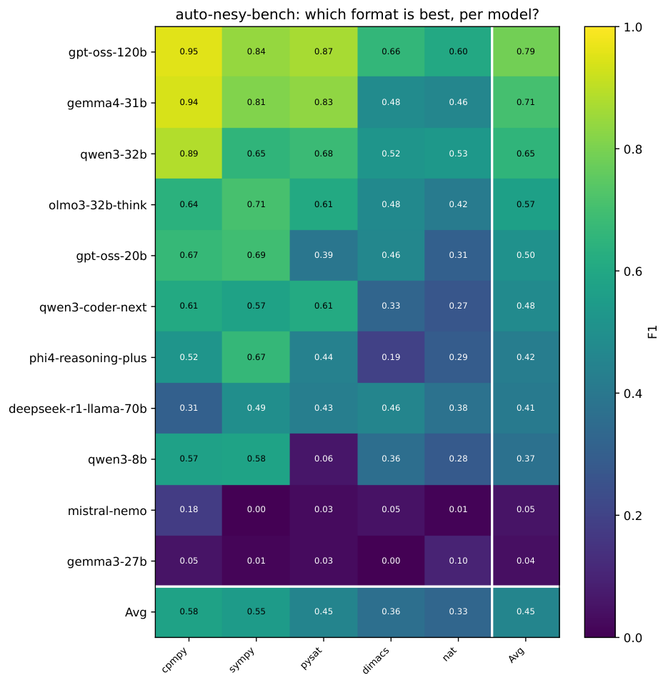


Code-based formats perform best on average on auto-nesy-bench. CPMpy achieves the highest across-model mean F1 at , followed by SymPy at . PySAT ranks third at , while direct DIMACS generation reaches and NAT performs worst at . Thus, compared with generating the final representation directly, the two strongest higher-level formats improve mean F1 by approximately -. This suggests that allowing models to generate a high-level symbolic program may make formalization easier than requiring them to construct the low-level DIMACS encoding directly, potentially because code is more prevalent in LLM training data.
However, the best output format varies across models. The strongest model overall on auto-nesy-bench, gpt-oss-120b, achieves its highest F1 with CPMpy (), compared with for PySAT, for SymPy, for DIMACS, and for NAT. In contrast, SymPy performs best for several other competitive models, including olmo3-32b-think (), gpt-oss-20b (), and qwen-8b (). qwen-coder-next performs similarly with PySAT () and CPMpy (). Thus, while CPMpy and SymPy are the strongest formats on average, choosing the format for a specific model can yield substantial additional gains.
A similar preference for code-based formats emerges on dcpbench, although the best format varies more substantially across models. Across models, CPMpy achieves the highest mean F1 (), followed by PySAT () and SymPy (). At the model level, however, deepseek-r1-llama-70b performs best with SymPy (), gpt-oss-120b with PySAT (), gpt-oss-20b with CPMpy (), and qwen-coder-next with CPMpy (). No single code-based format is therefore consistently best across models.
The pattern is different on satbench. Here, NAT is the strongest format on average across models, achieving an F1 of . It is also the strongest format for gpt-oss-120b () and qwen-coder-next (), while gemma4-31b performs best with CPMpy (), compared with for NAT. Thus, the advantage of code-based representations observed on auto-nesy-bench and dcpbench does not transfer uniformly across datasets.
Overall, these results show that no single output format consistently dominates across models and datasets. Higher-level code representations, particularly CPMpy and SymPy, perform well on auto-nesy-bench and dcpbench, whereas NAT is substantially stronger on satbench. The choice of output format should therefore be viewed as a model- and dataset-dependent factor in formalization performance.
I.1.4 Syntactic Error Analysis
Finally, we examine which errors most often prevent the auto-formalization pipeline from producing valid formulas and whether these errors differ across models and output formats. We focus on syntactic errors, including missing output delimiters, parsing errors, malformed DIMACS content, program-execution failures, and timeouts. The complete error taxonomy is provided in Appendix C.
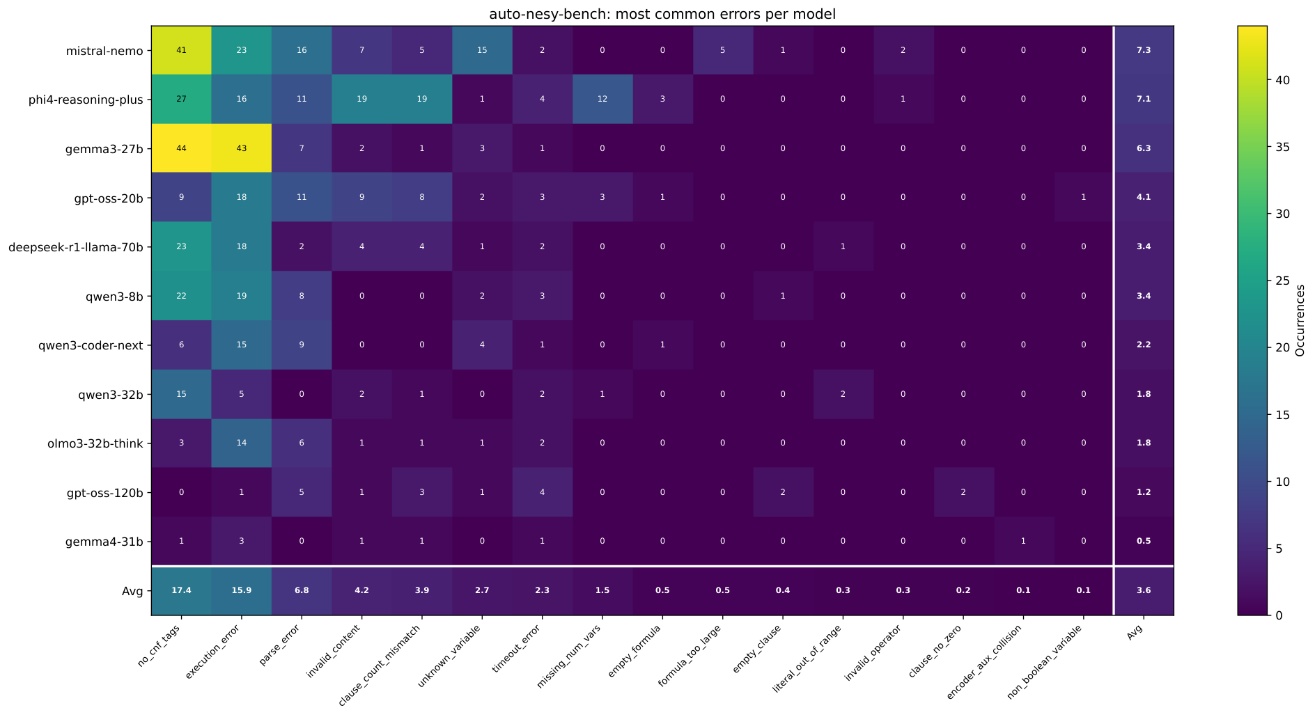


Figure 13 shows that errors are concentrated in a small number of categories and models. On auto-nesy-bench, no_cnf_tags is the most common error category, with occurrences, followed by execution_error (), parse_error (), invalid_content (), and clause_count_mismatch (). mistral-nemo has the most errors overall, with an average of errors per error type. This includes execution errors and missing-tag errors. phi4-reasoning-plus follows with an average of errors per type, while gemma3-27b averages , with execution errors and missing-tag errors. In contrast, gemma4-31b has only errors per type, and gpt-oss-120b has , with one execution error and no missing-tag errors. These results show that auto-formalization depends not only on the LLM reasoning ability, but also on its ability to follow formatting instructions and produce outputs that can be parsed and executed correctly. On dcpbench, execution errors are the most common category, averaging occurrences per model, followed by missing tags (), unknown variables (), and parsing errors (). gpt-oss-20b has the largest mean count across error types (), followed by deepseek-r1-llama-70b (), qwen3-coder-next (), and gpt-oss-120b (). On satbench, qwen3-coder-next has the most errors, with execution errors and an average of errors per type. In contrast, gpt-oss-120b has only three errors in total, with no execution errors. gemma4-31b has eleven errors: ten invalid-content errors and one execution error.
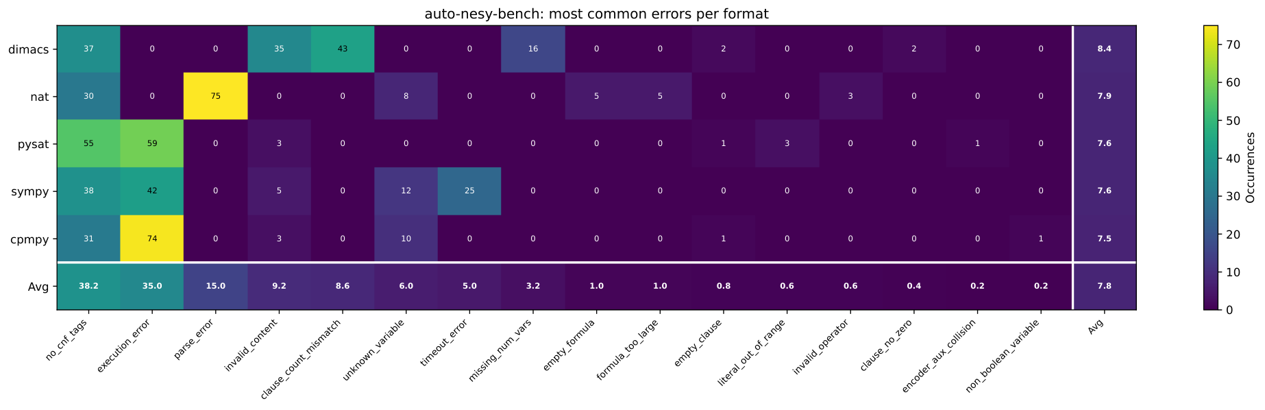


The format-level analysis in Fig. 14 shows that the types of errors vary substantially across output formats. On auto-nesy-bench, direct DIMACS generation has the highest mean count ( occurrences per error type), despite having the lowest syntax error rate, as a single output can contribute to multiple error codes. Its main errors are clause-count mismatches (), missing <cnf> tags (), and invalid content (). In contrast, NAT mainly fails during parsing ( errors), followed by missing tags (). Code-based formats largely avoid these errors but introduce execution failures: PySAT, CPMpy, and SymPy produce , , and execution errors, respectively. CPMpy has the lowest mean count overall (), while SymPy produces timeouts, suggesting that symbolic conversion can become a computational bottleneck. Missing <cnf> tags occur across all formats, ranging from to instances, indicating a general instruction-following issue. On dcpbench, PySAT has the lowest average number of errors (), while DIMACS has a higher average of . Clause-count mismatches () and invalid content () are still common errors. The NAT format has the highest mean count (), including parsing errors, while PySAT and CPMpy produce and execution errors, respectively. SymPy averages , including execution errors, unknown-variable errors, and timeouts. On satbench, DIMACS has the lowest mean count (), followed by NAT (). Execution errors dominate the code-based formats, with for CPMpy, for PySAT, and for SymPy; all are produced by qwen3-coder-next except for one CPMpy execution error from gemma4-31b. Overall, the types of errors depend on the output format. Higher-level formats reduce manual encoding errors but can cause more errors considering code execution, symbolic conversion, and computational cost.
I.2 Downstream Results of LLM-Generated Formulas on NeSy Predictors
In the following tables, we report the full evaluation results for the ground-truth formulas and the formulas generated by gpt-oss-120b, olmo3-32b-think, and qwen3-8b, as discussed in Section 5.2.
I.2.1 Downstream Results with Detailed Prompts on SPL
| Task | Consistency | Accuracy | Precision | Recall | F1 | Rel | MC-R |
|---|---|---|---|---|---|---|---|
| bdd-oia-2 | |||||||
| cebab | |||||||
| cifar10 | |||||||
| cifar100 | |||||||
| cle4evr | |||||||
| fashion | |||||||
| kand-logic-2 | |||||||
| mn-add | |||||||
| mn-mul-bin | |||||||
| mn-mul | |||||||
| sushi | |||||||
| warcraft |
| Task | Consistency | Accuracy | Precision | Recall | F1 | Rel | MC-R |
|---|---|---|---|---|---|---|---|
| bdd-oia | |||||||
| cifar10 | |||||||
| cifar100 | |||||||
| cle4evr | |||||||
| fashion | |||||||
| kand-logic-2 | |||||||
| mn-add-bin | |||||||
| mn-add | |||||||
| mn-mul | |||||||
| sudoku | |||||||
| sushi |
| Task | Consistency | Accuracy | Precision | Recall | F1 | Rel | MC-R |
|---|---|---|---|---|---|---|---|
| bdd-oia | |||||||
| bdd-oia-2 | |||||||
| cebab | |||||||
| chx | |||||||
| cifar10 | |||||||
| cifar100 | |||||||
| cle4evr | |||||||
| fashion | |||||||
| kand-logic | |||||||
| kand-logic-2 | |||||||
| mn-add-bin | |||||||
| mn-add | |||||||
| mn-mul-bin | |||||||
| mn-mul | |||||||
| road-r | |||||||
| sudoku | |||||||
| sushi | |||||||
| warcraft |
| Task | Consistency | Accuracy | Precision | Recall | F1 | Rel | MC-R |
|---|---|---|---|---|---|---|---|
| bdd-oia | |||||||
| bdd-oia-2 | |||||||
| cebab | |||||||
| chx | |||||||
| cifar10 | |||||||
| cifar100 | |||||||
| cle4evr | |||||||
| fashion | |||||||
| kand-logic | |||||||
| kand-logic-2 | |||||||
| mn-add-bin | |||||||
| mn-add | |||||||
| mn-mul-bin | |||||||
| mn-mul | |||||||
| road-r | |||||||
| sudoku | |||||||
| sushi | |||||||
| warcraft |
Failed attempts. Table 24 accounts for missing results in Table 4 and Table 30, all under the CPMpy +CoT configuration used throughout the SPL downstream evaluation. We distinguish three categories. Formula degenerate means a CNF was produced and compiles, but is unusable: either it is unsatisfiable (0 models, confirmed directly via model counting), or it declares variables the encoded constraint never actually uses, e.g., olmo3-32b-think/mn-add-bin formula, for instance, omits 4 of its 13 declared variables entirely, i.e., (sum_bit1-sum_bit4). No formula produced means the auto-formalization run for that (model, task, format, prompt) combination never emitted a usable CNF to begin with. Run failure means that a valid formula exist, but the run fails due to SDD compilation. Five of the thirteen errors are caused by incorrect formulas: olmo3-32b-think/bdd-oia, olmo3-32b-think/mn-add-bin, qwen3-8b/kand-logic, qwen3-8b/chx, and qwen3-8b/road-r.
| Model | Task | Category | Reason (CPMpy+CoT) |
| olmo3-32b-think | bdd-oia | formula degenerate | UNSAT (0 models) |
| olmo3-32b-think | kand-logic | no formula produced | no CNF generated |
| olmo3-32b-think | sudoku | no formula produced | no CNF generated |
| olmo3-32b-think | chx | run failure | CUDA device-side assert |
| olmo3-32b-think | road-r | run failure | process stalled |
| olmo3-32b-think | mn-add-bin | formula degenerate | 4 of 13 declared variables are missing |
| qwen3-8b | kand-logic | formula degenerate | UNSAT (0 models) |
| qwen3-8b | chx | formula degenerate | formula omits 1 of 9 oracle concept variables |
| qwen3-8b | bdd-oia-2 | no formula produced | no CNF generated |
| qwen3-8b | cebab | no formula produced | no CNF generated |
| qwen3-8b | warcraft | run failure | oracle/formula output-shape mismatch |
| qwen3-8b | mn-mul-bin | run failure | SDD compilation error |
| qwen3-8b | road-r | formula degenerate | UNSAT (0 models) |
I.2.2 What Happens When SPL Is Equipped with LLM-Generated Formulas from Less Detailed Prompts?
To study this ablation, we run the same experiment as for SPL in Section 5.2, but use a less fine-grained prompt description. This is possible because auto-nesy-bench is the only auto-formalization benchmark that supports this setting. Below, we compare the ground-truth model (which is the same as in Section 5.2) with the models trained under this setting.
Discussion. Table 25 shows the SPL results with CPMpy output using CoT and non-detailed prompt. In this setting, LLM-generated formulas are still usable in most cases, but they are much less likely to be exactly correct than when using detailed prompts (Table 4). Only about half of the usable formulas are equal to the ground-truth, i.e., Rel is ( for gpt-oss-120b, for olmo3-32b-think, and for qwen3-8b), whereas the remaining ones are mostly incomparable () or strict (). As a result, the generated formulas are farther from the ground-truth formula. The average F1 and recall are and for gpt-oss-120b, and for olmo3-32b-think, and and for qwen3-8b. With detailed prompts, these differences are less than and , respectively. This gap is mainly caused by non-equivalent formulas, which reduce F1 by – on average. As with detailed prompts, overly strict formulas are the most harmful. On kand-logic-2, the formulas produced by gpt-oss-120b and olmo3-32b-think capture only of the valid assignments (MC-R ), reducing F1 by and , respectively. incomparable formulas can be just as harmful. For example, gpt-oss-120b on cifar10 loses F1, while olmo3-32b-think loses on chx and on mn-add-bin. In contrast, over-approximations () have little effect. On cifar10, the formulas produced by olmo3-32b-think and qwen3-8b allow about more assignments than the ground truth, yet reduce F1 by only -. This suggests that the model can learn to down-weight these spurious output combinations during training. equal formulas perform almost as well as the ground truth on nearly all tasks. The main exception is sudoku, where F1 drops by - even though the formula is equivalent to the ground truth. Unlike with detailed prompts, predictions are no longer always consistent with the ground-truth constraints. incomparable and unknown formulas can allow assignments that the ground truth rejects, which lowers SPL consistency. For example, on road-r, consistency drops by , , and for gpt-oss-120b, olmo3-32b-think, and qwen3-8b, respectively. On kand-logic, it drops by for qwen3-8b. In contrast, strict and permissive formulas never produce inconsistent predictions. Failures are also more common for the strongest model: gpt-oss-120b fails on tasks, compared with with detailed prompts. olmo3-32b-think and qwen3-8b each fail on tasks. Most failures are caused by degenerate formulas that leave some task variables unconstrained or are unsatisfiable (see Table 29). Overall, these results show that the task specification matters as much as the choice of LLM. Detailed prompts are important for obtaining correct formulas and, consequently, SPL performance close to that achieved with expert-provided knowledge.
| G-T | gpt-oss-120b | olmo3-32b-think | |||||||||||
| Task | F1 | Rec | Cons | F1 | Rec | Cons | Rel | MC-R | F1 | Rec | Cons | Rel | MC-R |
| bdd-oia | – | – | – | – | – | – | – | – | – | – | |||
| bdd-oia-2 | – | – | – | – | – | ||||||||
| cebab | – | – | – | – | – | – | – | – | – | – | |||
| chx | |||||||||||||
| cifar10 | |||||||||||||
| cifar100 | |||||||||||||
| cle4evr | |||||||||||||
| fashion | |||||||||||||
| kand-logic | unknown | – | – | – | – | – | – | ||||||
| kand-logic-2 | |||||||||||||
| mn-add-bin | |||||||||||||
| mn-add | |||||||||||||
| mn-mul-bin | – | – | – | – | – | ||||||||
| mn-mul | |||||||||||||
| road-r | |||||||||||||
| sudoku | |||||||||||||
| sushi | |||||||||||||
| warcraft | – | – | – | – | – | ||||||||
| G-T | qwen3-8b | |||||||
| Task | F1 | Rec | Cons | F1 | Rec | Cons | Rel | MC-R |
| bdd-oia | – | – | – | – | – | |||
| bdd-oia-2 | – | – | – | – | – | |||
| cebab | – | – | – | – | – | |||
| chx | – | – | – | – | – | |||
| cifar10 | ||||||||
| cifar100 | ||||||||
| cle4evr | ||||||||
| fashion | ||||||||
| kand-logic | unknown | – | ||||||
| kand-logic-2 | ||||||||
| mn-add-bin | ||||||||
| mn-add | ||||||||
| mn-mul-bin | ||||||||
| mn-mul | – | – | – | – | – | |||
| road-r | ||||||||
| sudoku | ||||||||
| sushi | ||||||||
| warcraft | – | – | – | – | – | |||
| Task | Consistency | Accuracy | Precision | Recall | F1 | Rel | MC-R |
|---|---|---|---|---|---|---|---|
| bdd-oia-2 | |||||||
| chx | |||||||
| cifar10 | |||||||
| cifar100 | |||||||
| cle4evr | |||||||
| fashion | |||||||
| kand-logic | unknown | – | |||||
| kand-logic-2 | |||||||
| mn-add-bin | |||||||
| mn-add | |||||||
| mn-mul-bin | |||||||
| mn-mul | |||||||
| road-r | |||||||
| sudoku | |||||||
| sushi | |||||||
| warcraft |
| Task | Consistency | Accuracy | Precision | Recall | F1 | Rel | MC-R |
|---|---|---|---|---|---|---|---|
| chx | |||||||
| cifar10 | |||||||
| cifar100 | |||||||
| cle4evr | |||||||
| fashion | |||||||
| kand-logic-2 | |||||||
| mn-add-bin | |||||||
| mn-add | |||||||
| mn-mul | |||||||
| road-r | |||||||
| sudoku | |||||||
| sushi |
| Task | Consistency | Accuracy | Precision | Recall | F1 | Rel | MC-R |
|---|---|---|---|---|---|---|---|
| cifar10 | |||||||
| cifar100 | |||||||
| cle4evr | |||||||
| fashion | |||||||
| kand-logic | unknown | – | |||||
| kand-logic-2 | |||||||
| mn-add-bin | |||||||
| mn-add | |||||||
| mn-mul-bin | |||||||
| road-r | |||||||
| sudoku | |||||||
| sushi |
Failed attempts (non-detailed prompts). Table 29 accounts for the missing results in Table 25, using the same CPMpy +CoT configuration but with non-detailed prompts. We use the same three categories as for detailed prompts (Table 24). Most errors are now formula-degenerate ( out of ). In bdd-oia, all three models omit part of the scene description: gpt-oss-120b never uses of the variables (follow, left_follow, no_left_lane, right_follow, no_right_lane), while olmo3-32b-think and qwen3-8b omit . On bdd-oia-2, both smaller models also drop the follow concept. The qwen3-8b formula for mn-mul omits of its variables, corresponding exactly to the product classes that no pair of digits can produce (e.g., p_11, p_13, and p_17). Rather than explicitly constraining these variables to false, the formula leaves them unconstrained. Two formulas are unsatisfiable: olmo3-32b-think/warcraft and qwen3-8b/cebab. Finally, the qwen3-8b formula for chx admits only a single assignment, leaving no parameters in the compiled circuit for SPL to learn. The remaining four gaps are no formula produced: cebab for gpt-oss-120b and olmo3-32b-think, kand-logic and mn-mul-bin for olmo3-32b-think, and warcraft for qwen3-8b. Unlike with detailed prompts, there are no run failures: every usable formula is trained successfully. With detailed prompts, gpt-oss-120b produced a usable formula for every task. Without them, even the strongest model fails on tasks, and failures for all models are more often caused by incorrect formulas than by pipeline issues. This suggests that, without a detailed specification, LLMs tend to under-specify the constraints rather than fail to produce a formula altogether.
| Model | Task | Category | Reason (CPMpy+CoT, non-detailed prompt) |
|---|---|---|---|
| gpt-oss-120b | bdd-oia | formula degenerate | 5 of 25 task variables are missing |
| gpt-oss-120b | cebab | no formula produced | no CNF generated |
| olmo3-32b-think | bdd-oia | formula degenerate | 6 of 25 task variables are missing |
| olmo3-32b-think | bdd-oia-2 | formula degenerate | 1 of 11 task variables is missing |
| olmo3-32b-think | warcraft | formula degenerate | UNSAT (0 models) |
| olmo3-32b-think | cebab | no formula produced | no CNF generated |
| olmo3-32b-think | kand-logic | no formula produced | no CNF generated |
| olmo3-32b-think | mn-mul-bin | no formula produced | no CNF generated |
| qwen3-8b | bdd-oia | formula degenerate | 6 of 25 task variables are missing |
| qwen3-8b | bdd-oia-2 | formula degenerate | 1 of 11 task variables is missing |
| qwen3-8b | cebab | formula degenerate | UNSAT (0 models) |
| qwen3-8b | mn-mul | formula degenerate | 45 of 102 task variables are missing |
| qwen3-8b | chx | formula degenerate | no trainable circuit parameters |
| qwen3-8b | warcraft | no formula produced | no CNF generated |
I.2.3 What if the Constraints are Soft? Semantic Loss Downstream Results with Detailed Prompts
In addition to the SPL results, we further analyze the downstream performance under a different NeSy approach based on the semantic loss (SL) (Xu et al., 2018), which incorporates logical constraints as a penalty loss rather than explicitly enforcing them during prediction. Specifically, we replicate the same SPL analysis (CPMpy +CoT and detailed prompt in Section 5.2) using the SL.
Semantic Loss. Given an input and an unconstrained predictive distribution , SL (Xu et al., 2018) incorporates a logical constraint by maximizing the probability mass assigned to its satisfying assignments. Assuming conditional independence of the variables given the model outputs, it is defined as
| (16) |
where is the number of primary Boolean output variables. For a Boolean variable, is a shorthand for if and otherwise. Thus, the sum computes the total probability assigned to all satisfying assignments, and the negative logarithm penalizes the model when this probability is low. The sum in Eq. 16 is exactly the weighted model count (WMC) (Chavira and Darwiche, 2008) of under the weights induced by .
Implementation. For these experiments, we reuse the same SDDs compiled for the SPL experiments. At training time, the SDD is loaded using KLay (Maene et al., 2025), which makes the WMC, and hence of , faster. Unlike SPL, which explicitly incorporates logical constraints into the prediction mechanism, SL treats as a soft constraint through an additional differentiable loss term. In our setting, it is combined with the downstream task objective as
| (17) |
where controls the strength of the logical constraint. As all the benchmarks in auto-nesy-bench are classification tasks, corresponds to the negative log-likelihood, while for all SL experiments is set to .
Architectures. SL uses the same per-task backbones as SPL. We only replace the SPL head, which outputs the parameters of the circuit, with a classification head: an MLP with three hidden layers with ReLU activations, whose width is set to the SPL head width tuned for that task, and one output per variable of the CNF. Each output is passed through a sigmoid, so that factorizes into independent Bernoulli distributions over the variables; this is the distribution on which computes the probability of satisfying , with the positive and negative literal weights given by and . At test time, each variable is predicted by thresholding its probability at ; for tasks with a single multi-class output, we predict the class whose output-bit pattern is most likely.
Discussion. Table 30 reports the SL experiments in the same setting as Section 5.2, i.e., using the formulas generated by the LLMs with detailed prompts, chain-of-thought, and CPMpy as output format. Without SL, the unconstrained network is often inconsistent with the ground-truth formula: its consistency is below on seven of the tasks, ranging from on sushi and on sudoku to on warcraft, whereas simpler tasks such as cle4evr, fashion, and the mn datasets are already almost fully consistent (). Adding the SL with an equivalent formula () never decreases consistency and increases it on all tasks that leave room for improvement, most notably on sushi, where it rises from to -, and on road-r and cebab ( to ). Unlike SPL (see Section 5.2), however, whose predictions satisfy the formula by construction, SL only encourages consistency during training, and it rarely reaches : on the hardest tasks it remains far from it (kand-logic -, sudoku -). Downstream performance, for equal () formulas, is almost unaffected by the semantic loss (mean F1 between and across LLMs), with gains concentrated on the most constrained tasks (sudoku, to F1; mn-mul-bin, up to ). The only formula that reduces consistency is the one generated by qwen3-8b for kand-logic-2 ( Cons, F1). This formula is too strict (): it admits only of the assignments allowed by the ground truth (MC-R ), so it rules out most of the labels seen during training. Interestingly, as for SPL, permissive formulas () are much less harmful: on warcraft, the formulas of gpt-oss-120b and olmo3-32b-think still improve consistency by and , respectively. Probably the classification loss also contributes by assigning low probability mass on invalid combinations.
| Unconstrained | G-T | gpt-oss-120b | |||||||||||
|---|---|---|---|---|---|---|---|---|---|---|---|---|---|
| Task | F1 | Rec | Cons | F1 | Rec | Cons | Rel | MC-R | F1 | Rec | Cons | Rel | MC-R |
| bdd-oia | |||||||||||||
| bdd-oia-2 | |||||||||||||
| cebab | |||||||||||||
| chx | |||||||||||||
| cifar10 | |||||||||||||
| cifar100 | |||||||||||||
| cle4evr | |||||||||||||
| fashion | |||||||||||||
| kand-logic | |||||||||||||
| kand-logic-2 | |||||||||||||
| mn-add-bin | |||||||||||||
| mn-add | |||||||||||||
| mn-mul-bin | |||||||||||||
| mn-mul | |||||||||||||
| road-r | |||||||||||||
| sudoku | |||||||||||||
| sushi | |||||||||||||
| warcraft | |||||||||||||
| Unconstrained | olmo3-32b-think | qwen3-8b | |||||||||||
| Task | F1 | Rec | Cons | F1 | Rec | Cons | Rel | MC-R | F1 | Rec | Cons | Rel | MC-R |
| bdd-oia | – | – | – | – | – | ||||||||
| bdd-oia-2 | – | – | – | – | – | ||||||||
| cebab | – | – | – | – | – | ||||||||
| chx | – | – | – | – | – | – | – | – | – | – | |||
| cifar10 | |||||||||||||
| cifar100 | |||||||||||||
| cle4evr | |||||||||||||
| fashion | |||||||||||||
| kand-logic | – | – | – | – | – | – | – | – | – | – | |||
| kand-logic-2 | |||||||||||||
| mn-add-bin | – | – | – | – | – | ||||||||
| mn-add | |||||||||||||
| mn-mul-bin | – | – | – | – | – | ||||||||
| mn-mul | |||||||||||||
| road-r | – | – | – | – | – | – | – | – | – | – | |||
| sudoku | – | – | – | – | – | ||||||||
| sushi | |||||||||||||
| warcraft | – | – | – | – | – | ||||||||
| Task | Consistency | Accuracy | Precision | Recall | F1 |
|---|---|---|---|---|---|
| bdd-oia | |||||
| bdd-oia-2 | |||||
| cebab | |||||
| chx | |||||
| cifar10 | |||||
| cifar100 | |||||
| cle4evr | |||||
| fashion | |||||
| kand-logic | |||||
| kand-logic-2 | |||||
| mn-add-bin | |||||
| mn-add | |||||
| mn-mul-bin | |||||
| mn-mul | |||||
| road-r | |||||
| sudoku | |||||
| sushi | |||||
| warcraft |
| Task | Consistency | Accuracy | Precision | Recall | F1 | Rel | MC-R |
|---|---|---|---|---|---|---|---|
| bdd-oia | |||||||
| bdd-oia-2 | |||||||
| cebab | |||||||
| chx | |||||||
| cifar10 | |||||||
| cifar100 | |||||||
| cle4evr | |||||||
| fashion | |||||||
| kand-logic | |||||||
| kand-logic-2 | |||||||
| mn-add-bin | |||||||
| mn-add | |||||||
| mn-mul-bin | |||||||
| mn-mul | |||||||
| road-r | |||||||
| sudoku | |||||||
| sushi | |||||||
| warcraft |
| Task | Consistency | Accuracy | Precision | Recall | F1 | Rel | MC-R |
|---|---|---|---|---|---|---|---|
| bdd-oia | |||||||
| bdd-oia-2 | |||||||
| cebab | |||||||
| chx | |||||||
| cifar10 | |||||||
| cifar100 | |||||||
| cle4evr | |||||||
| fashion | |||||||
| kand-logic | |||||||
| kand-logic-2 | |||||||
| mn-add-bin | |||||||
| mn-add | |||||||
| mn-mul-bin | |||||||
| mn-mul | |||||||
| road-r | |||||||
| sudoku | |||||||
| sushi | |||||||
| warcraft |
| Task | Consistency | Accuracy | Precision | Recall | F1 | Rel | MC-R |
|---|---|---|---|---|---|---|---|
| bdd-oia-2 | |||||||
| cebab | |||||||
| cifar10 | |||||||
| cifar100 | |||||||
| cle4evr | |||||||
| fashion | |||||||
| kand-logic-2 | |||||||
| mn-add | |||||||
| mn-mul-bin | |||||||
| mn-mul | |||||||
| sushi | |||||||
| warcraft |
| Task | Consistency | Accuracy | Precision | Recall | F1 | Rel | MC-R |
|---|---|---|---|---|---|---|---|
| bdd-oia | |||||||
| cifar10 | |||||||
| cifar100 | |||||||
| cle4evr | |||||||
| fashion | |||||||
| kand-logic-2 | |||||||
| mn-add-bin | |||||||
| mn-add | |||||||
| mn-mul | |||||||
| sudoku | |||||||
| sushi |
I.2.4 Soft Constraints with Semantic Loss equipped with LLM-Generated Formulas from Less Detailed Prompts
As for SPL in Section I.2.2, we replicate the same exact analysis for SL, i.e., CPMpy with CoT and less detailed prompts.
| Unconstrained | G-T | gpt-oss-120b | |||||||||||
|---|---|---|---|---|---|---|---|---|---|---|---|---|---|
| Task | F1 | Rec | Cons | F1 | Rec | Cons | Rel | MC-R | F1 | Rec | Cons | Rel | MC-R |
| bdd-oia | – | – | – | – | – | ||||||||
| bdd-oia-2 | |||||||||||||
| cebab | – | – | – | – | – | ||||||||
| chx | |||||||||||||
| cifar10 | |||||||||||||
| cifar100 | |||||||||||||
| cle4evr | |||||||||||||
| fashion | |||||||||||||
| kand-logic | unknown | – | |||||||||||
| kand-logic-2 | |||||||||||||
| mn-add-bin | |||||||||||||
| mn-add | |||||||||||||
| mn-mul-bin | |||||||||||||
| mn-mul | |||||||||||||
| road-r | |||||||||||||
| sudoku | |||||||||||||
| sushi | |||||||||||||
| warcraft | |||||||||||||
| Unconstrained | olmo3-32b-think | qwen3-8b | |||||||||||
| Task | F1 | Rec | Cons | F1 | Rec | Cons | Rel | MC-R | F1 | Rec | Cons | Rel | MC-R |
| bdd-oia | – | – | – | – | – | – | – | – | – | – | |||
| bdd-oia-2 | – | – | – | – | – | – | – | – | – | – | |||
| cebab | – | – | – | – | – | – | – | – | – | – | |||
| chx | – | – | |||||||||||
| cifar10 | |||||||||||||
| cifar100 | |||||||||||||
| cle4evr | |||||||||||||
| fashion | |||||||||||||
| kand-logic | – | – | – | – | – | unknown | – | ||||||
| kand-logic-2 | |||||||||||||
| mn-add-bin | |||||||||||||
| mn-add | |||||||||||||
| mn-mul-bin | – | ||||||||||||
| mn-mul | – | – | – | – | – | ||||||||
| road-r | |||||||||||||
| sudoku | |||||||||||||
| sushi | |||||||||||||
| warcraft | – | – | – | – | – | – | – | – | – | – | |||
Discussion. Table 36 propose the same SL experiments from Table 30 but using formulas generated from non-detailed prompts. equal formulas () behave similarly to those generated from detailed prompts: they never reduce consistency by more than and provide the same gains on all the tasks, e.g., sushi ( to Cons) and sudoku ( to Cons, to F1), while leaving downstream performance mostly unaffected. However, only about half of the produced formulas are exactly correct (, , and for gpt-oss-120b, olmo3-32b-think, and qwen3-8b, respectively), and the non-equal formulas are often harmful. With detailed prompts, only a single formula reduced consistency; here, the strict and incomparable formulas reduce consistency on most of the tasks, often by a large margin: kand-logic-2 ( to Cons for all three models), chx ( for olmo3-32b-think), mn-add-bin ( for olmo3-32b-think), road-r ( for qwen3-8b), and cifar10 ( for gpt-oss-120b). These formulas also reduce F1, e.g., by up to for qwen3-8b/chx, whose formula admits only a single assignment of the concepts. Unlike SPL, however, SL can still be trained with such a formula as it is used as a loss function. The reason is the same as for the too-strict formula in Table 30. If the formula excludes some assignments that are actually present in the training data, the two losses give conflicting signals: the classification loss encourages the model to predict the ground-truth assignments, while the semantic loss pushes it away from them because they violate the formula. The model therefore ends up in a compromise that may satisfy neither the formula nor the ground-truth labels. As a result, the average consistency gain of SL over the unconstrained model drops from about with detailed prompts to for gpt-oss-120b and qwen3-8b, and becomes negative for olmo3-32b-think (). The mean F1 ranges from to . Permissive formulas () remain harmless, as with detailed prompts and for SPL. On cifar10, formulas admitting about more assignments than the ground truth still slightly improve consistency (). Similarly, the permissive gpt-oss-120b formula for warcraft improves both F1 () and consistency (), since a superset of the valid assignments can still exclude some invalid ones. Overall, SL is more robust than SPL to imperfect formulas because it uses the formula as a soft training signal rather than enforcing it on every prediction. As a result, incorrect formulas do not necessarily prevent training, although they can still hurt performance when they conflict with the ground truth.
| Task | Consistency | Accuracy | Precision | Recall | F1 | Rel | MC-R |
|---|---|---|---|---|---|---|---|
| chx | – | – | |||||
| cifar10 | |||||||
| cifar100 | |||||||
| cle4evr | |||||||
| fashion | |||||||
| kand-logic | unknown | – | |||||
| kand-logic-2 | |||||||
| mn-add-bin | |||||||
| mn-add | |||||||
| mn-mul-bin | |||||||
| road-r | |||||||
| sudoku | |||||||
| sushi |
| Task | Consistency | Accuracy | Precision | Recall | F1 | Rel | MC-R |
|---|---|---|---|---|---|---|---|
| chx | |||||||
| cifar10 | |||||||
| cifar100 | |||||||
| cle4evr | |||||||
| fashion | |||||||
| kand-logic-2 | |||||||
| mn-add-bin | |||||||
| mn-add | |||||||
| mn-mul | |||||||
| road-r | |||||||
| sudoku | |||||||
| sushi |
| Task | Consistency | Accuracy | Precision | Recall | F1 | Rel | MC-R |
|---|---|---|---|---|---|---|---|
| bdd-oia-simple | |||||||
| chx | |||||||
| cifar10 | |||||||
| cifar100 | |||||||
| cle4evr | |||||||
| fashion- | |||||||
| kand-logic | unknown | – | |||||
| kand-logic-2 | |||||||
| mn-add-bin | |||||||
| mn-add | |||||||
| mn-mul-bin | |||||||
| mn-mul | |||||||
| road-r | |||||||
| sudoku | |||||||
| sushi | |||||||
| warcraft |