跳到论文正文
W Papers独立论文阅读器 arXiv:2610.01474 论文正文 计算阅读时间 · 0%
引用这篇论文根据当前论文元数据生成,正式投稿前建议核对。


License: CC BY 4.0
arXiv:2610.01474v1 [eess.SP] 01 Oct 2026

Cramér-Rao Bound Optimization for Joint Beamforming and Mode Selection in RDARS-Assisted ISAC Systems

Ahmad Reza Hassanshahi    Rouhollah Amiri    Fereidoon Behnia
Abstract

Integrated Sensing and Communication (ISAC) is a foundation of 6G networks, demanding architectures that simultaneously enhance sensing accuracy and communication reliability. This paper presents a Reconfigurable Distributed Antenna and Reflecting Surface (RDARS) aided ISAC framework, where an RDARS overcomes the limitations of conventional passive Reconfigurable Intelligent Surfaces (RIS) and Distributed Antenna Systems (DAS). By enabling each element to dynamically operate in either reflection or connection mode, RDARS synergistically harnesses reflection gain, distribution gain, and an additional mode-selection gain. We investigate the joint optimization of transmit beamforming at the base station and dynamic mode selection at the RDARS to minimize the sensing performance metric, namely the Cramér-Rao Bound (CRB) for target localization, while guaranteeing a minimum required Signal-to-Interference-plus-Noise Ratio (SINR) for multiple communication users. To solve the resulting non-convex and mixed-integer problem, we develop an efficient iterative algorithm based on the Alternating Optimization (AO) framework, effectively leveraging Majorization-Minimization (MM) and Penalty methods. Comprehensive simulations validate the proposed design, demonstrating that the dynamic RDARS configuration achieves a superior trade-off between the Position Error Bound (PEB) and communication SINR, significantly outperforming benchmark passive RIS and DAS systems.

Index Terms: 
Integrated Sensing and Communication (ISAC), Reconfigurable Distributed Antennas and Reflecting Surface (RDARS), Reconfigurable Intelligent Surface (RIS), Signal-to-Interference-plus-Noise Ratio (SINR), Cramér-Rao Bound (CRB), beamforming, mode selection.

I Introduction

The relentless advancement towards 6G networks is characterized by a strategic migration to higher frequency bands, such as mmWave and Terahertz. This transition unlocks a paradigm where radio signals transcend their traditional role, facilitating not only high-speed data transmission but also the acquisition of high-resolution information about the surrounding environment [1, 2, 3, 4]. This convergence is formalized in Integrated Sensing and Communication (ISAC), a key enabling technology that effectively optimizes spectral and hardware resources by consolidating sensing and communication functionalities [5, 6, 7, 8, 9, 10]. Emerging applications, including autonomous navigation, smart cities, and industrial automation, demand not merely connectivity but an elevated capacity for environmental perception and comprehension [5]. ISAC is thus poised to be integral to 6G, providing the critical real-time environmental awareness required for these applications [5]. Furthermore, architectures like the Distributed Antenna Systems (DAS) and its evolutions (e.g., cell-free massive MIMO), which distribute network elements to reduce access distance, can provide a foundational infrastructure conducive to the deployment of sophisticated ISAC frameworks, despite challenges related to power and complexity [11, 12].

I-A Related Works

The design of ISAC systems fundamentally involves a trade-off between communication performance and sensing accuracy, often quantified by distinct metrics. On the communication side, common objectives are the maximization of the sum rate [13, 14] or the guaranteeing of a minimum Signal-to-Interference-plus-Noise Ratio (SINR) for each user [15, 16]. Conversely, sensing performance is frequently evaluated through the maximization of radar Signal-to-Clutter-plus-Noise Ratio [17, 18], beamforming gain towards targets [19, 20], or the minimization of the Cramér-Rao Bound (CRB) [21, 22], which provides a lower bound on the variance of unbiased estimators for sensing parameters like target direction or distance. The system architecture plays a pivotal role in managing these trade-offs. While DAS and their evolutions offer a distribution gain, they incur high power consumption and hardware costs [11, 12]. Reconfigurable Intelligent Surface (RIS) has emerged as a low-cost alternative to reshape the wireless environment [23, 24]. Subsequent variants like Simultaneously Transmitting and Reflecting RIS (STAR-RIS) [25, 26] and Hybrid Relay-RIS (HR-RIS) [27, 28] have been developed to overcome inherent limitations such as limited coverage and the multiplicative fading effect. Recent research has extensively explored the integration of these surfaces into ISAC, focusing on joint beamforming design for both fully-passive RIS and active/hybrid variants to balance communication and sensing objectives [21, 22, 29, 30, 31, 32, 33, 34]. To harness the benefits of both DAS and RIS, the novel Reconfigurable Distributed Antennas and Reflecting Surfaces (RDARS) architecture was proposed in [35]. The RDARS, whose elements operating in either connected or reflected mode, achieves a hybrid distribution and reflection gain. After the preliminary work in [35], RDARS has begun to explore its potential by designing an active/passive beamformer in MIMO communication systems [36, 37] and investigating the trade-off between rate and SNR in an RDARS-aided ISAC system [38]. However, a critical gap remains unaddressed: the integration of RDARS within an ISAC framework optimized for sensing accuracy via the CRB. To the best of our knowledge, no existing work has jointly optimized transmit beamforming and RDARS configuration to minimize the position CRB for target localization under stringent communication QoS constraints. While [38] studies RDARS-aided ISAC using sensing SINR, our work adopts the position-domain CRB as the localization metric. Recent closely related developments include an RDARS ISAC/localization demonstration, hybrid-RIS mode-selection designs, active-RIS CRB optimization, and tri-mode RDARS-ISAC waveform/mode switching [39, 40, 41, 42]. None of these works addresses the joint connected/reflected RDARS mode selection and transmit design for position-CRB minimization under multi-user SINR constraints. In the proposed formulation, the RDARS configuration changes both the communication channel and the geometry-dependent Fisher information contributed by the BS/RDARS-target paths. This localization-oriented coupling, rather than the use of standard AO/MM tools by itself, is the main technical distinction from prior RDARS-ISAC designs.

I-B Contributions

This paper jointly optimizes transmit beamforming and dynamic mode selection in an RDARS-aided ISAC system to minimize the CRB while ensuring multi-user SINR. The NP-hard problem, involving variable coupling and unit-modulus/binary constraints, is addressed via an Alternating Optimization (AO) framework combining relaxation, successive approximation/MM, and penalty methods. Simulations confirm its superiority over passive RIS and DAS benchmarks in beampattern, geometry, and Position Error Bound (PEB)-SINR trade-off. The main contributions are:

  • •

    Tractable SINR and CRB expressions as functions of active beamforming 𝐅\mathbf{F}, reflection coefficients 𝚽\bm{\Phi}, and mode selection 𝐀\mathbf{A}, enabling a concrete problem formulation.

  • •

    An efficient AO-based iterative algorithm decomposing the problem into sub-problems, with MM/successive approximation handling non-convexities and penalty terms enforcing SINR and mode-selection consistency.

  • •

    Extensive simulations evaluating beampatterns, geometry, and sensing-communication trade-off. The proposed RDARS outperforms passive RIS and DAS, achieving lower PEB under same SINR constraints by exploiting hybrid distribution and reflection gains.

I-C Outline

The remainder of this paper is organized as follows. Section II presents the RDARS-assisted ISAC system model, including communication and radar channels, and defines the SINR and CRB metrics. Section III derives the CRB via the FIM, establishing the theoretical lower bound for localization accuracy. Section IV formulates the joint beamforming and mode selection problem and develops an AO-based solution integrating MM and penalty techniques. Section V provides simulation results, including beampatterns, trade-off analyses, geometric evaluations, and parametric studies, to validate the superiority of the proposed scheme over benchmarks in terms of PEB and SINR. Finally, Section VI concludes the paper.

Notations: Scalars, vectors, and matrices are denoted by italic, bold lowercase, and bold uppercase letters, respectively. For a matrix 𝐀\mathbf{A}, (⋅)T(\cdot)^{T}, (⋅)∗(\cdot)^{*}, (⋅)H(\cdot)^{H}, and tr⁡(⋅)\operatorname{tr}(\cdot) denote transpose, conjugate, conjugate-transpose, and trace; 𝐀⁡(i,j)\mathbf{A}(i,j) denotes its (i,j)(i,j)-th entry, and ‖𝐀‖F\|\mathbf{A}\|_{F} is the Frobenius norm. diag⁡(𝐚)\operatorname{diag}(\mathbf{a}) forms a diagonal matrix from vector 𝐚\mathbf{a}, blkdiag⁡(⋅)\mathrm{blkdiag}(\cdot) forms a block-diagonal matrix, and vec⁡(⋅)\operatorname{vec}(\cdot) denotes vectorization. For a complex number, |⋅||\cdot| is the modulus and ∥⋅∥\|\cdot\| the Euclidean norm; ℜ⁡{⋅}\Re\{\cdot\} and ℑ⁡{⋅}\Im\{\cdot\} extract real and imaginary parts. 𝔼​{⋅}\mathbb{E}\{\cdot\} denotes statistical expectation, and 𝒞​𝒩​(𝝁,𝚺)\mathcal{CN}(\bm{\mu},\mathbf{\Sigma}) represents a CSCG distribution. ℝa×b\mathbb{R}^{a\times b} and ℂa×b\mathbb{C}^{a\times b} denote the sets of a×ba\times b real and complex matrices, respectively. 𝐈\mathbf{I} and 𝐎\mathbf{O} are the identity and zero matrices, whose dimensions are clear from the context.

II Problem Formulation And System Model

II-A Scenario Description

We consider an ISAC system comprising a Base Station (BS), KK single-antenna users, a target and an RDARS panel, operating under MIMO-OFDM signaling with NsN_{s} subcarriers and the subcarrier spacing Δ​f\Delta f. We use centered frequency indices n∈𝒩s≜{−(Ns−1)/2,…,(Ns−1)/2}n\in\mathcal{N}_{s}\triangleq\{-(N_{s}-1)/2,\ldots,(N_{s}-1)/2\}; for even NsN_{s}, these are half-integer offsets with respect to the band center. The objective is to accurately sense and locate the target while ensuring user communications remain at a desirable level. The performance is evaluated using the communication SINR and the radar CRB metrics. A schematic of the scenario is shown in Fig. 1.

The BS, equipped with Mt=Mr=MM_{t}=M_{r}=M antennas arranged in a Uniform Linear Array (ULA), concurrently serves KK users and detects a point target. The RDARS consists of NN elements arranged in a Uniform Planar Array (UPA) configuration, each dynamically switchable between two modes: reflected mode (passive phase shifting) and connected mode (active transmission and reception). Only a≪Na\ll N elements operate in connected mode for hardware efficiency. The binary diagonal matrix 𝐀=diag⁡{a1,…,aN}\mathbf{A}=\mathrm{diag}\{a_{1},\dots,a_{N}\} indicates the mode of each element (ai=1a_{i}=1 for connected, ai=0a_{i}=0 for reflected). The reflection coefficients are modeled by 𝚽=diag⁡{ϕ1,…,ϕN}\bm{\Phi}=\mathrm{diag}\{\phi_{1},\dots,\phi_{N}\}, where ϕi=|ϕi|​ej​arg​(ϕi)\phi_{i}=|\phi_{i}|e^{j\mathrm{arg}(\phi_{i})} with arg⁡(ϕi)∈[0,2​π)\mathrm{arg}({\phi}_{i})\in[0,2\pi) and |ϕi|=1|\phi_{i}|=1. The overall RDARS reflection effect is captured by (𝐈−𝐀)​𝚽(\mathbf{I}-\mathbf{A})\bm{\Phi}. In downlink, the BS and connected RDARS elements act as a distributed antenna system. The transmitted signal is

𝐗⁡[n]=[𝐱1​[n]𝐱2​[n]]=[𝐅1𝐅2]​𝐬​[n]≜𝐅𝐬⁡[n],∀n∈𝒩s.\mathbf{X}[n]=\scalebox{0.9}{$\begin{bmatrix}\mathbf{x}_{1}[n]\\ \mathbf{x}_{2}[n]\end{bmatrix}=\begin{bmatrix}\mathbf{F}_{1}\\ \mathbf{F}_{2}\end{bmatrix}\mathbf{s}[n]\triangleq\mathbf{F}\mathbf{s}[n]$},\quad\scalebox{0.9}{$\forall n\in\mathcal{N}_{s}$}. (1)

where 𝐬⁡[n]∼𝒞​𝒩​(𝟎,𝐈K)\mathbf{s}[n]\sim\mathcal{CN}(\mathbf{0},\mathbf{I}_{K}) contains user data symbols, and 𝐅1∈ℂM×K\mathbf{F}_{1}\in\mathbb{C}^{M\times K} and 𝐅2∈ℂa×K\mathbf{F}_{2}\in\mathbb{C}^{a\times K} are beamforming matrices at the BS and RDARS connected elements, respectively, and we define 𝐑X​1\mathbf{R}_{X1} and 𝐑X​2\mathbf{R}_{X2} as follows:

𝐑X​1=𝐅1​𝐅1H,𝐑X​2=𝐅2​𝐅2H.\mathbf{R}_{X1}=\scalebox{0.9}{$\mathbf{F}_{1}\mathbf{F}_{1}^{H},\quad\quad\mathbf{R}_{X2}=\mathbf{F}_{2}\mathbf{F}_{2}^{H}$}. (2)

II-B Communication Channel

The communication channels in the considered system are defined as follows. Let 𝐇b​r∈ℂN×M\mathbf{H}_{br}\in\mathbb{C}^{N\times M} represent the channel matrix between the BS and RDARS, 𝐡b​u,k∈ℂM\mathbf{h}_{bu,k}\in\mathbb{C}^{M} denote the channel vector from the BS to the kk-th user, and 𝐡r​u,k∈ℂN\mathbf{h}_{ru,k}\in\mathbb{C}^{N} signify the channel vector from the RDARS to the kk-th user. All channel components are characterized by a general Rician fading model. Specifically, the BS-RDARS channel 𝐇b​r\mathbf{H}_{br} is expressed as

𝐇b​r=αb​r​(κ​𝐇b​rLoS+1−κ​𝐇b​rNLoS),\mathbf{H}_{br}=\scalebox{0.9}{$\sqrt{\alpha_{br}}\left(\sqrt{\kappa}\,\mathbf{H}_{br}^{\text{LoS}}+\sqrt{1-\kappa}\,\mathbf{H}_{br}^{\text{NLoS}}\right)$}, (3)

where αb​r\alpha_{br} is the path loss coefficient, κ\kappa denotes the Rician factor, 𝐇b​rNLoS\mathbf{H}_{br}^{\text{NLoS}} represents the non-line-of-sight (NLoS) component whose entries are independent and identically distributed (i.i.d.) complex Gaussian random variables, i.e., 𝐇b​rNLoS​(i,j)∼𝒞​𝒩​(0,1)\mathbf{H}_{br}^{\text{NLoS}}(i,j)\sim\mathcal{CN}(0,1), and 𝐇b​rLoS\mathbf{H}_{br}^{\text{LoS}} is the deterministic line-of-sight (LoS) component.

Considering the described system model, the received signal at the kk-th user can be formulated as:

𝐘u,k​[n]\displaystyle\mathbf{Y}_{u,k}[n] =(𝐡b​u,kT+𝐡r​u,kT​(𝐈−𝐀)​𝚽​𝐇b​r)​𝐱1​[n]+𝐡r​u,kT​𝐀a​𝐱2​[n]+𝐙C,k​[n]\displaystyle=\scalebox{0.8}{$\displaystyle\left(\mathbf{h}_{bu,k}^{T}+\mathbf{h}_{ru,k}^{T}(\mathbf{I}-\mathbf{A})\bm{\Phi}\mathbf{H}_{br}\right)\mathbf{x}_{1}[n]+\mathbf{h}_{ru,k}^{T}\mathbf{A}_{a}\mathbf{x}_{2}[n]+\mathbf{Z}_{C,k}[n]$}
=𝐡kT​𝐅𝐬​[n]+𝐙C,k​[n],\displaystyle=\scalebox{0.95}{$\mathbf{h}_{k}^{T}\mathbf{F}\mathbf{s}[n]+\mathbf{Z}_{C,k}[n]$}, (4)

where 𝐡k=[𝐡b​u,kT+𝐡r​u,kT(𝐈−𝐀)𝚽𝐇b​r,𝐡r​u,kT𝐀a]T\mathbf{h}_{k}=\left[\mathbf{h}_{bu,k}^{T}+\mathbf{h}_{ru,k}^{T}(\mathbf{I}-\mathbf{A})\bm{\Phi}\mathbf{H}_{br},\quad\mathbf{h}_{ru,k}^{T}\mathbf{A}_{a}\right]^{T} represents the composite communication channel from the BS and the RDARS’s connected elements to the kk-th user, and 𝐙C,k​[n]∼𝒞​𝒩​(𝟎,σk2)\mathbf{Z}_{C,k}[n]\sim\mathcal{CN}(\mathbf{0},\mathbf{\sigma}^{2}_{k}) is the additive white Gaussian noise (AWGN). It is important to highlight the introduction of an additional selection matrix 𝐀a∈ℝN×a\mathbf{A}_{a}\in\mathbb{R}^{N\times a} in (4), which is employed to handle the dimensionality mismatch between the signal vectors 𝐱1​[n]\mathbf{x}_{1}[n] and 𝐱2​[n]\mathbf{x}_{2}[n]. Specifically, 𝐀a\mathbf{A}_{a} is constructed by extracting the aa columns from the master selection matrix 𝐀\mathbf{A} that correspond to the connected-mode elements. This relationship can be compactly expressed as 𝐀=𝐀a​𝐀aT\mathbf{A}=\mathbf{A}_{a}\mathbf{A}_{a}^{\mathrm{T}}.

Based on the received communication signal model (4), the SINR for the kk-th user can be formulated as:

SINRu,k=|𝐡kT​𝐟k|2∑i≠kK|𝐡kT​𝐟i|2+σk2,\textbf{SINR}_{u,k}=\frac{\left|\mathbf{h}_{k}^{\mathrm{T}}\mathbf{f}_{k}\right|^{2}}{\sum_{i\neq k}^{K}\left|\mathbf{h}_{k}^{\mathrm{T}}\mathbf{f}_{i}\right|^{2}+\sigma_{k}^{2}}, (5)

where 𝐟i\mathbf{f}_{i} denotes the ii-th column of the composite beamforming matrix 𝐅\mathbf{F}, for i=1,…,Ki=1,\ldots,K, representing the beamforming vector dedicated to user ii.

Refer to caption

Fig. 1: The system model of an RDARS-aided ISAC system.

II-C Radar Channel

This section analyzes the received radar signal. As shown in Fig. 1, the radar channel comprises five distinct propagation paths:

  1. 1.

    BS →\to Target →\to BS Path: The signal travels directly from the BS to the target and back to the BS.

  2. 2.

    BS →\to Target →\to RDARS Path: The signal propagates from the BS to the target and is then reflected back to the RDARS’s connected elements.

  3. 3.

    BS →\to Target →\to RDARS →\to BS Path: The signal travels from the BS to the target and is then reflected to the RDARS’s reflection elements and is finally reflected back to the BS.

  4. 4.

    RDARS →\to Target →\to RDARS Path: The signal is transmitted from the RDARS’s connected elements to the target and returns to the RDARS.

  5. 5.

    RDARS →\to Target →\to BS Path: The signal transmitted from the connected elements of RDARS to the target and is then reflected back to the BS.

The BS, located at 𝐪∈ℝ2\mathbf{q}\in\mathbb{R}^{2}, serves KK single-antenna users at 𝐮∈ℝ2\mathbf{u}\in\mathbb{R}^{2} while sensing a point target at 𝐩∈ℝ2\mathbf{p}\in\mathbb{R}^{2}, aided by an RDARS at 𝐫∈ℝ2\mathbf{r}\in\mathbb{R}^{2}. The total received radar signal for subcarrier nn is given by:

𝐘R​[n]=[α1​e−j​2​π​n​Δ​f​τ1​𝐆1​𝐱1​[n]+α3​e−j​2​π​n​Δ​f​τ3​𝐆3​𝐱1​[n]+α5​e−j​2​π​n​Δ​f​τ5​𝐆5​𝐱2​[n]α2​e−j​2​π​n​Δ​f​τ2​𝐆2​𝐱1​[n]+α4​e−j​2​π​n​Δ​f​τ4​𝐆4​𝐱2​[n]]+𝐙R​[n],\mathbf{Y}_{R}[n]=\begin{bmatrix}\alpha_{1}e^{-j2\pi n\Delta f\tau_{1}}{\mathbf{G}}_{1}\mathbf{x}_{1}[n]\\ +\alpha_{3}e^{-j2\pi n\Delta f\tau_{3}}{\mathbf{G}}_{3}\mathbf{x}_{1}[n]\\ +\alpha_{5}e^{-j2\pi n\Delta f\tau_{5}}{\mathbf{G}}_{5}\mathbf{x}_{2}[n]\\ \alpha_{2}e^{-j2\pi n\Delta f\tau_{2}}{\mathbf{G}}_{2}\mathbf{x}_{1}[n]\\ +\alpha_{4}e^{-j2\pi n\Delta f\tau_{4}}{\mathbf{G}}_{4}\mathbf{x}_{2}[n]\end{bmatrix}+\mathbf{Z}_{R}[n],\\ (6)

where the path delays are:

τ1\displaystyle\tau_{1} =2c​‖𝐪−𝐩‖2,\displaystyle=\scalebox{0.9}{$\frac{2}{c}\|\mathbf{q}-\mathbf{p}\|_{2}$}, (7)
τ2\displaystyle\tau_{2} =τ5=1c​[‖𝐫−𝐩‖2+‖𝐪−𝐩‖2],\displaystyle=\tau_{5}=\scalebox{0.9}{$\frac{1}{c}\left[\|\mathbf{r}-\mathbf{p}\|_{2}+\|\mathbf{q}-\mathbf{p}\|_{2}\right]$}, (8)
τ3\displaystyle\tau_{3} =1c​[‖𝐪−𝐫‖2+‖𝐫−𝐩‖2+‖𝐩−𝐪‖2],\displaystyle=\scalebox{0.9}{$\frac{1}{c}\left[\|\mathbf{q}-\mathbf{r}\|_{2}+\|\mathbf{r}-\mathbf{p}\|_{2}+\|\mathbf{p}-\mathbf{q}\|_{2}\right]$}, (9)
τ4\displaystyle\tau_{4} =2c​‖𝐫−𝐩‖2.\displaystyle=\scalebox{0.9}{$\frac{2}{c}\|\mathbf{r}-\mathbf{p}\|_{2}$}. (10)

The term Δ​f\Delta f denotes the subcarrier spacing and 𝐙R​[n]∼𝒞​𝒩​(𝟎,σ2​𝐈)\mathbf{Z}_{R}[n]\sim\mathcal{CN}(\mathbf{0},\sigma^{2}\mathbf{I}) represents AWGN. The parameters αk\alpha_{k} denote the complex path gains. Here, θ1\theta_{1} is the BS-target angle, θ2\theta_{2} is the RDARS-target direction in a global frame, θ3\theta_{3} is the BS-RDARS angle in the BS frame, θ4\theta_{4} is the RDARS-BS angle in the RDARS frame, and θ5\theta_{5} is the same RDARS-target direction expressed in the RDARS local frame. The array orientations are assumed known, so θ5=θ2+ψ0\theta_{5}=\theta_{2}+\psi_{0} for a known frame offset ψ0\psi_{0}, and therefore ∂θ5/∂θ2=1\partial\theta_{5}/\partial\theta_{2}=1. The beamforming gain matrices 𝐆k\mathbf{G}_{k} are defined as follows: 𝐆1=𝐚⁡(θ1)​𝐚H​(θ1)\mathbf{G}_{1}=\mathbf{a}(\theta_{1})\mathbf{a}^{H}(\theta_{1}), 𝐆2=𝐀aT​𝐛​(θ2)​𝐚H​(θ1)\mathbf{G}_{2}=\mathbf{A}_{a}^{T}\mathbf{b}(\theta_{2})\mathbf{a}^{H}(\theta_{1}), 𝐆3=g​𝐚​(θ1)​𝐚H​(θ3)\mathbf{G}_{3}=g\,\mathbf{a}(\theta_{1})\mathbf{a}^{H}(\theta_{3}), 𝐆4=𝐀aT​𝐛​(θ2)​𝐛H​(θ2)​𝐀a\mathbf{G}_{4}=\mathbf{A}_{a}^{T}\mathbf{b}(\theta_{2})\mathbf{b}^{H}(\theta_{2})\mathbf{A}_{a}, and 𝐆5=𝐚⁡(θ1)​𝐛H​(θ2)​𝐀a\mathbf{G}_{5}=\mathbf{a}(\theta_{1})\mathbf{b}^{H}(\theta_{2})\mathbf{A}_{a}. Where 𝐚⁡(⋅)\mathbf{a}(\cdot) denotes the BS array response and 𝐛eff​(⋅)=𝐀aT​𝐛full​(⋅)\mathbf{b}_{\text{eff}}(\cdot)=\mathbf{A}_{a}^{T}\mathbf{b}_{\text{full}}(\cdot) represents the effective array response of the connected RDARS elements. The gain factor gg for path 3 is computed as follows (where 𝐜⁡(⋅)\mathbf{c}(\cdot) corresponds to the RDARS reflected elements array response):

g=𝐜H​(θ4)​[(𝐈−𝐀)​𝚽]​𝐜​(θ5).g=\mathbf{c}^{H}(\theta_{4})\left[(\mathbf{I}-\mathbf{A})\bm{\Phi}\right]\mathbf{c}(\theta_{5}). (11)

II-D Performance Metrics

To evaluate and compare different systems, appropriate performance metrics must be defined. For ISAC systems, these typically fall into two categories: communication metrics (e.g., data rate or SINR) and radar metrics (e.g., target localization accuracy). In this work, we adopt the SINR as the communication metric and the CRB as the radar performance metric. The CRB provides a fundamental lower bound on the covariance matrix of any unbiased estimator [43]. Based on the received signal model in (6), the complete parameter vector 𝜸∈ℝ12\bm{\gamma}\in\mathbb{R}^{12} includes both the target position and the path loss coefficients is given by 𝜸=[𝐩T,𝜶T]T\bm{\gamma}=[\mathbf{p}^{T},\bm{\alpha}^{T}]^{T}, where 𝜶=[𝜶1T,𝜶2T,𝜶3T,𝜶4T,𝜶5T]T\bm{\alpha}=[\bm{\alpha}_{1}^{T},\bm{\alpha}_{2}^{T},\bm{\alpha}_{3}^{T},\bm{\alpha}_{4}^{T},\bm{\alpha}_{5}^{T}]^{T} and each sub-vector 𝜶k\bm{\alpha}_{k} contains the real and imaginary parts of the path loss coefficient for the kk-th path, i.e., 𝜶k=[ℜ⁡{αk},ℑ⁡{αk}]T\bm{\alpha}_{k}=[\Re\{\alpha_{k}\},\Im\{\alpha_{k}\}]^{T}.

Let 𝜸^\hat{\bm{\gamma}} be an estimate of 𝜸\bm{\gamma} obtained from the observations 𝐘R​[n]\mathbf{Y}_{R}[n]’s. The Mean Squared Error (MSE) matrix satisfies the inequality [43]:

𝔼⁡{(𝜸^−𝜸)​(𝜸^−𝜸)T}≥𝐉𝜸−1,\scalebox{0.9}{$\mathbb{E}\left\{(\hat{\bm{\gamma}}-\bm{\gamma})(\hat{\bm{\gamma}}-\bm{\gamma})^{T}\right\}\geq\mathbf{J}_{\bm{\gamma}}^{-1}$}, (12)

where 𝐉𝜸\mathbf{J}_{\bm{\gamma}} is the FIM for 𝜸\bm{\gamma}. In particular, for the target position estimate 𝐩^\hat{\mathbf{p}}, (12) yields a lower bound on the localization MSE:

𝔼⁡{(𝐩^−𝐩)​(𝐩^−𝐩)T}≥CRB​(𝐩).\scalebox{0.9}{$\mathbb{E}\left\{(\hat{\mathbf{p}}-\mathbf{p})(\hat{\mathbf{p}}-\mathbf{p})^{T}\right\}\geq\textrm{CRB}(\mathbf{p})$}. (13)

III Calculation of the CRB of Target Position

This section analyzes the fundamental limits of target localization by deriving the corresponding FIM. Following the received signal model in (6), the complete parameter vector 𝜸∈ℝ12\bm{\gamma}\in\mathbb{R}^{12} is defined to encapsulate both the target position and the path loss coefficients:

𝜸=[𝐩T,𝜶T]T,\bm{\gamma}=[\mathbf{p}^{T},\bm{\alpha}^{T}]^{T}, (14)

where 𝜶=[𝜶1T,𝜶2T,𝜶3T,𝜶4T,𝜶5T]T\bm{\alpha}=[\bm{\alpha}_{1}^{T},\bm{\alpha}_{2}^{T},\bm{\alpha}_{3}^{T},\bm{\alpha}_{4}^{T},\bm{\alpha}_{5}^{T}]^{T}. Each sub-vector 𝜶k\bm{\alpha}_{k} comprises the real and imaginary parts of the path loss coefficient for the kk-th path, i.e., 𝜶k=[ℜ⁡{αk},ℑ⁡{αk}]T\bm{\alpha}_{k}=[\Re\{\alpha_{k}\},\Im\{\alpha_{k}\}]^{T}.

To simplify the analysis, we introduce a reparameterization from 𝜸\bm{\gamma} to an intermediate vector 𝜼=[𝝉T,𝜽T,𝜶T]T∈ℝ17\bm{\eta}=[\bm{\tau}^{T},\bm{\theta}^{T},\bm{\alpha}^{T}]^{T}\in\mathbb{R}^{17}, where 𝝉=[τ1,τ2,τ3,τ4,τ5]T\bm{\tau}=[\tau_{1},\tau_{2},\tau_{3},\tau_{4},\tau_{5}]^{T} contains the time delays and 𝜽=[θ1,θ2]T\bm{\theta}=[\theta_{1},\theta_{2}]^{T}. For the compact closed-form expressions below, we adopt a resolvable-path approximation: distinct paths are separable over the OFDM/array observation aperture, the centered subcarrier indexing above is used, and the relevant delay/gain and angle/gain score inner products vanish. Under this stated approximation,

𝐉𝜼=blkdiag⁡[𝐉τ,𝐉θ,𝐉α].\mathbf{J}_{\bm{\eta}}=\operatorname{blkdiag}[\mathbf{J}_{\tau},\mathbf{J}_{\theta},\mathbf{J}_{\alpha}]. (15)

If these orthogonality conditions are not satisfied, the full FIM must be retained and the position EFIM is obtained directly from the Schur complement in (23). Under the adopted approximation, the required diagonal terms are:

Jτi,τi\displaystyle J_{\tau_{i},\tau_{i}} =2σ2|αi|2(2πΔf)2tr{𝐆i𝐑x​1𝐆iH}∑n=−(Ns−1)/2(Ns−1)/2n2,i=1,2,3\displaystyle=\scalebox{0.81}{$\frac{2}{\sigma^{2}}|\alpha_{i}|^{2}(2\pi\Delta f)^{2}\mathrm{tr}\{\mathbf{G}_{i}\mathbf{R}_{x1}\mathbf{G}_{i}^{H}\}\sum_{n=-(N_{s}-1)/2}^{(N_{s}-1)/2}n^{2}$},\quad\scalebox{0.81}{$i=1,2,3$} (16)
Jτj,τj\displaystyle J_{\tau_{j},\tau_{j}} =2σ2|αj|2(2πΔf)2tr{𝐆j𝐑x​2𝐆jH}∑n=−(Ns−1)/2(Ns−1)/2n2,j=4,5\displaystyle=\scalebox{0.81}{$\frac{2}{\sigma^{2}}|\alpha_{j}|^{2}(2\pi\Delta f)^{2}\mathrm{tr}\{\mathbf{G}_{j}\mathbf{R}_{x2}\mathbf{G}_{j}^{H}\}\sum_{n=-(N_{s}-1)/2}^{(N_{s}-1)/2}n^{2}$},\quad\scalebox{0.81}{$j=4,5$} (17)
Jθ1,θ1\displaystyle J_{\theta_{1},\theta_{1}} =2​Nsσ2​(∑k∈{1,2,3}|αk|2​tr​{𝐆˙k,θ1​𝐑x​1​𝐆˙k,θ1H}+|α5|2​tr​{𝐆˙5,θ1​𝐑x​2​𝐆˙5,θ1H}),\displaystyle=\scalebox{0.7}{$\frac{2{N}_{s}}{\sigma^{2}}\Bigg(\sum_{k\in\{1,2,3\}}|\alpha_{k}|^{2}\,\mathrm{tr}\{\dot{\mathbf{G}}_{k,\theta_{1}}\mathbf{R}_{x1}\dot{\mathbf{G}}_{k,\theta_{1}}^{H}\}+|\alpha_{5}|^{2}\,\mathrm{tr}\{\dot{\mathbf{G}}_{5,\theta_{1}}\mathbf{R}_{x2}\dot{\mathbf{G}}_{5,\theta_{1}}^{H}\}\Bigg)$}, (18)
Jθ2,θ2\displaystyle J_{\theta_{2},\theta_{2}} =2​Nsσ2​(|α2|2​tr⁡{𝐆˙2,θ2​𝐑x​1​𝐆˙2,θ2H}+|α3|2​tr⁡{𝐆˙3,θ2​𝐑x​1​𝐆˙3,θ2H}CLOSE\displaystyle=\scalebox{0.74}{$\frac{2N_{s}}{\sigma^{2}}\Big(|\alpha_{2}|^{2}\operatorname{tr}\{\dot{\mathbf{G}}_{2,\theta_{2}}\mathbf{R}_{x1}\dot{\mathbf{G}}_{2,\theta_{2}}^{H}\}+|\alpha_{3}|^{2}\operatorname{tr}\{\dot{\mathbf{G}}_{3,\theta_{2}}\mathbf{R}_{x1}\dot{\mathbf{G}}_{3,\theta_{2}}^{H}\}$}
OPEN+|α4|2​tr⁡{𝐆˙4,θ2​𝐑x​2​𝐆˙4,θ2H}+|α5|2​tr⁡{𝐆˙5,θ2​𝐑x​2​𝐆˙5,θ2H}),\displaystyle\quad\scalebox{0.74}{$+|\alpha_{4}|^{2}\operatorname{tr}\{\dot{\mathbf{G}}_{4,\theta_{2}}\mathbf{R}_{x2}\dot{\mathbf{G}}_{4,\theta_{2}}^{H}\}+|\alpha_{5}|^{2}\operatorname{tr}\{\dot{\mathbf{G}}_{5,\theta_{2}}\mathbf{R}_{x2}\dot{\mathbf{G}}_{5,\theta_{2}}^{H}\}\Big)$}, (19)
Jαi,αi\displaystyle J_{\alpha_{i},\alpha_{i}} =2σ2​tr​{𝐆i​𝐑x​1​𝐆iH}​Ns​𝐈2,i=1,2,3\displaystyle=\scalebox{0.78}{$\frac{2}{\sigma^{2}}\mathrm{tr}\{\mathbf{G}_{i}\mathbf{R}_{x1}\mathbf{G}_{i}^{H}\}{N}_{s}\mathbf{I}_{2}$},\quad\scalebox{0.81}{$i=1,2,3$} (20)
Jαj,αj\displaystyle J_{\alpha_{j},\alpha_{j}} =2σ2​tr​{𝐆j​𝐑x​2​𝐆jH}​Ns​𝐈2,j=4,5\displaystyle=\scalebox{0.78}{$\frac{2}{\sigma^{2}}\mathrm{tr}\{\mathbf{G}_{j}\mathbf{R}_{x2}\mathbf{G}_{j}^{H}\}{N}_{s}\mathbf{I}_{2}$},\quad\scalebox{0.81}{$j=4,5$} (21)

where 𝐆i\mathbf{G}_{i} are the beamforming gain matrices, and 𝐆˙i,θk\dot{\mathbf{G}}_{i,\theta_{k}} denotes the derivative of 𝐆i\mathbf{G}_{i} with respect to θk\theta_{k}. In particular, 𝐆˙3,θ2\dot{\mathbf{G}}_{3,\theta_{2}} includes the dependence of gg on θ5=θ2+ψ0\theta_{5}=\theta_{2}+\psi_{0}. Under the same resolvable-path/orthogonality approximation, Jθ1,θ2=0J_{\theta_{1},\theta_{2}}=0. To obtain the position EFIM, we must eliminate the nuisance parameters. The full FIM for 𝜸\bm{\gamma} is partitioned as:

𝐉𝜸=[𝐉p​p𝐉p​α𝐉α​p𝐉α​α],\mathbf{J}_{\bm{\gamma}}=\begin{bmatrix}\mathbf{J}_{pp}&\mathbf{J}_{p\alpha}\\ \mathbf{J}_{\alpha p}&\mathbf{J}_{\alpha\alpha}\end{bmatrix}, (22)

where 𝐉p​p\mathbf{J}_{pp} corresponds to the position parameters, 𝐉α​α\mathbf{J}_{\alpha\alpha} corresponds to the path gains, and 𝐉p​α=𝐉α​pT\mathbf{J}_{p\alpha}=\mathbf{J}_{\alpha p}^{T} represents the coupling between them. The position EFIM is then obtained via the Schur complement:

𝐉e=𝐉p​p−𝐉p​α​𝐉α​α−1​𝐉α​p.\mathbf{J}_{e}=\scalebox{0.9}{$\mathbf{J}_{pp}-\mathbf{J}_{p\alpha}\mathbf{J}_{\alpha\alpha}^{-1}\mathbf{J}_{\alpha p}$}. (23)

Under the resolvable-path and score-orthogonality approximation stated above, the position–gain information block vanishes, i.e., 𝐉p​α=𝐎\mathbf{J}_{p\alpha}=\mathbf{O}, and the Schur complement reduces to:

𝐉e=𝐉p​p=𝚵T​𝐉m​𝚵,\mathbf{J}_{e}=\scalebox{0.9}{$\mathbf{J}_{pp}=\bm{\Xi}^{T}\mathbf{J}_{m}\bm{\Xi}$}, (24)

where 𝐉𝒎=blkdiag⁡[𝐉τ,𝐉θ]\mathbf{J}_{\bm{m}}=\operatorname{blkdiag}[\mathbf{J}_{\tau},\mathbf{J}_{\theta}] and the components 𝚵\bm{\Xi} and 𝐓\mathbf{T} (with 𝐓\mathbf{T} being the Jacobian transformation matrix) are defined in (69). The position-related submatrix denoted as effective FIM is given by:

𝐉e=𝚵T​𝐉m​𝚵=[J1,1J1,2J1,2J2,2].\mathbf{J}_{e}=\scalebox{0.9}{$\bm{\Xi}^{T}\mathbf{J}_{m}\bm{\Xi}$}=\scalebox{0.9}{$\begin{bmatrix}J_{1,1}&J_{1,2}\\ J_{1,2}&J_{2,2}\end{bmatrix}$}. (25)

Identifiability of the target position requires 𝐉e=𝐉p​p−𝐉p​α​𝐉α​α−1​𝐉α​p≻0\mathbf{J}_{e}=\mathbf{J}_{pp}-\mathbf{J}_{p\alpha}\mathbf{J}_{\alpha\alpha}^{-1}\mathbf{J}_{\alpha p}\succ 0. Degeneracy occurs whenever the available delay/angle score vectors fail to span both position dimensions, for example when distinct paths become locally indistinguishable or the transmit design places a sensing null toward the target. Collinearity can degrade conditioning for some geometries, but is not asserted here to be singular in every case. The CRB is well-defined for the simulated configurations for which 𝐉e\mathbf{J}_{e} is positive definite (Fig. 7). Clutter can be modeled as colored noise 𝐑n=σ2​𝐈+𝐑c\mathbf{R}_{n}=\sigma^{2}\mathbf{I}+\mathbf{R}_{c}, extending the framework via σ2​𝐈→𝐑c+σ2​𝐈\sigma^{2}\mathbf{I}\to\mathbf{R}_{c}+\sigma^{2}\mathbf{I}. Moreover, dynamic RCS can be addressed via chance constraints, as demonstrated in recent ISAC literature [44, 45], which enhance robustness to RCS fluctuations. These extensions are identified as future work. Finally, the CRB of target position is given by:

CRB=tr⁡(𝐉e−1)=J1,1+J2,2J1,1​J2,2−J1,22=𝐫H​𝐦+𝐦H​𝐫𝐫H​𝐁~​𝐫,\begin{split}\text{CRB}=\operatorname{tr}(\mathbf{J}_{e}^{-1})=\frac{J_{1,1}+J_{2,2}}{J_{1,1}J_{2,2}-J_{1,2}^{2}}=\frac{\mathbf{r}^{H}\mathbf{m}+\mathbf{m}^{H}\mathbf{r}}{\mathbf{r}^{H}\tilde{\mathbf{B}}\mathbf{r}},\end{split} (26)

where we have defined the unified vector 𝐫=[𝐫1T,𝐫2T]T∈ℂM2+a2\mathbf{r}=[\mathbf{r}_{1}^{T},\mathbf{r}_{2}^{T}]^{T}\in\mathbb{C}^{M^{2}+a^{2}} with 𝐫1≜vec​(𝐑X​1)\mathbf{r}_{1}\triangleq\text{vec}(\mathbf{R}_{X1}) and 𝐫2≜vec​(𝐑X​2)\mathbf{r}_{2}\triangleq\text{vec}(\mathbf{R}_{X2}). The parameters 𝐦\mathbf{m} and 𝐁~\tilde{\mathbf{B}} are defined in (86) and (87). The details of the CRB calculation, are provided in Appendix A.

IV Joint Beamforming and Mode Selection

IV-A Problem Formulation

This paper aims to enhance target positioning accuracy while guaranteeing multi-user communication performance. We formulate an optimization problem that minimizes the CRB under strict SINR constraints, jointly optimizing the composite transmit beamforming matrix 𝐅\mathbf{F}, the RDARS reflection matrix 𝚽\bm{\Phi}, and the selection matrices 𝐀\mathbf{A} and 𝐀a\mathbf{A}_{a}. Using the SINR and CRB analyses in (5) and (26), the detailed optimization problem is formulated as:

(P1) min𝐅,𝚽,𝐫,𝐀,𝐀a𝐫H​𝐦+𝐦H​𝐫𝐫H​𝐁~​𝐫\displaystyle\min_{\mathbf{F},\bm{\Phi},\mathbf{r},\mathbf{A},\mathbf{A}_{a}}\quad\scalebox{0.9}{$\frac{\mathbf{r}^{H}\mathbf{m}+\mathbf{m}^{H}\mathbf{r}}{\mathbf{r}^{H}\tilde{\mathbf{B}}\mathbf{r}}$}
s.t. 𝐫1=vec⁡(∑k=1K𝐅1,k),\displaystyle\mathbf{r}_{1}=\scalebox{0.9}{$\operatorname{vec}\left(\sum_{k=1}^{K}\mathbf{F}_{1,k}\right)$}, (27a)
𝐫2=vec⁡(∑k=1K𝐅2,k),\displaystyle\mathbf{r}_{2}=\scalebox{0.9}{$\operatorname{vec}\left(\sum_{k=1}^{K}\mathbf{F}_{2,k}\right)$}, (27b)
|𝐡kT​[𝐟1,k𝐟2,k]|2−γ¯k​∑i≠kK|𝐡kT​[𝐟1,i𝐟2,i]|2≥γ¯k​σk2,\displaystyle\scalebox{0.9}{$\left|\mathbf{h}_{k}^{T}\begin{bmatrix}\mathbf{f}_{1,k}\\ \mathbf{f}_{2,k}\end{bmatrix}\right|^{2}-\overline{\gamma}_{k}\sum_{i\neq k}^{K}\left|\mathbf{h}_{k}^{T}\begin{bmatrix}\mathbf{f}_{1,i}\\ \mathbf{f}_{2,i}\end{bmatrix}\right|^{2}\geq\overline{\gamma}_{k}\sigma_{k}^{2}$}, (27c)
‖𝐅‖F2≤Pt,\displaystyle\scalebox{0.9}{$\|\mathbf{F}\|_{F}^{2}\leq P_{t}$}, (27d)
|𝚽⁡(i,i)|=1,∀i,\displaystyle\scalebox{0.9}{$|\bm{\Phi}(i,i)|=1,\quad\forall i$}, (27e)
𝐀=𝐀a​𝐀aT,\displaystyle\scalebox{0.9}{$\mathbf{A}=\mathbf{A}_{a}\mathbf{A}_{a}^{T}$}, (27f)
𝐀(i,i)∈{0,1},i=1,…,N,\displaystyle\scalebox{0.9}{$\mathbf{A}(i,i)\in\{0,1\},\quad i=1,\dots,N$}, (27g)
tr⁡(𝐀)=a,\displaystyle\scalebox{0.9}{$\operatorname{tr}(\mathbf{A})=a$}, (27h)

where 𝐫=[𝐫1T,𝐫2T]T\mathbf{r}=[\mathbf{r}_{1}^{T},\mathbf{r}_{2}^{T}]^{T} and 𝐅=[𝐅1T,𝐅2T]T\mathbf{F}=[\mathbf{F}_{1}^{T},\mathbf{F}_{2}^{T}]^{T}. In optimization problem (P1), constraints (27a) and (27b) represent the vectorization of the submatrices of 𝐅\mathbf{F}. Constraint (27c) ensures that each user kk achieves a minimum SINR threshold γ¯k\overline{\gamma}_{k}. Constraint (27d) imposes a total power budget PtP_{t}, while (27e) enforces unit-modulus reflection coefficients. Constraints (27f), (27g), and (27h) define the feasible set for the mode selection matrices.

Problem (P1) is non-convex and challenging. To address this, we employ an AO framework that decomposes the problem into tractable sub-problems solved iteratively, integrating MM and penalty techniques. The procedure alternates between optimizing the beamforming matrix 𝐅\mathbf{F} with fixed 𝐀,𝐀a\mathbf{A},\mathbf{A}_{a}, and 𝚽\bm{\Phi}, and optimizing the reflection coefficients 𝚽\bm{\Phi} along with the mode selection matrices 𝐀\mathbf{A} and 𝐀a\mathbf{A}_{a} with fixed 𝐅\mathbf{F}.

IV-B Transmit Beamforming Matrix Optimization

This section presents the proposed methodology for the joint design of beamforming, phase, and mode selection in the RDARS-aided ISAC system.

For fixed 𝚽\bm{\Phi}, 𝐀\mathbf{A}, and 𝐀a\mathbf{A}_{a}, the optimization problem with respect to 𝐅\mathbf{F} is given by

(P2) min𝐅,𝐫𝐫H​𝐦+𝐦H​𝐫𝐫H​𝐁~​𝐫\displaystyle\min_{\mathbf{F},\mathbf{r}}\quad\frac{\mathbf{r}^{H}\mathbf{m}+\mathbf{m}^{H}\mathbf{r}}{\mathbf{r}^{H}\tilde{\mathbf{B}}\mathbf{r}}
s.t. (27a),(27b),(27c),(27d).\displaystyle\eqref{eq:r1-vec},\eqref{eq:r2-vec},\eqref{eq:sinr},\eqref{eq:power}. (28a)

Let us define 𝐅1,k≜𝐟1,k​𝐟1,kH\mathbf{F}_{1,k}\triangleq\mathbf{f}_{1,k}\mathbf{f}_{1,k}^{H}, 𝐅2,k≜𝐟2,k​𝐟2,kH\mathbf{F}_{2,k}\triangleq\mathbf{f}_{2,k}\mathbf{f}_{2,k}^{H}, 𝐅12,k≜𝐟1,k​𝐟2,kH\mathbf{F}_{12,k}\triangleq\mathbf{f}_{1,k}\mathbf{f}_{2,k}^{H}, and 𝐇k≜𝐡k∗​𝐡kT\mathbf{H}_{k}\triangleq\mathbf{h}_{k}^{*}\mathbf{h}_{k}^{T}. Thus, the beamforming optimization problem (P2) can be reformulated as

(P3)min𝐫1,𝐫2,(𝐅1,k)k=1K,(𝐅2,k)k=1K,(𝐅12,k)k=1K⁡𝐫H​𝐦+𝐦H​𝐫𝐫H​𝐁~​𝐫\displaystyle\text{(P3)}\quad\min_{\begin{subarray}{c}\mathbf{r}_{1},\mathbf{r}_{2},{(\mathbf{F}_{1,k})}_{k=1}^{K},\\ {(\mathbf{F}_{2,k})}_{k=1}^{K},{(\mathbf{F}_{12,k})}_{k=1}^{K}\end{subarray}}\scalebox{0.9}{$\frac{\mathbf{r}^{H}\mathbf{m}+\mathbf{m}^{H}\mathbf{r}}{\mathbf{r}^{H}\tilde{\mathbf{B}}\mathbf{r}}$}
s.t.(27a),(27b),\displaystyle\text{s.t.}\quad\quad\quad\eqref{eq:r1-vec},\eqref{eq:r2-vec}, (29a)
∑k=1Ktr⁡{[𝐅1,k𝐅12,k𝐅12,kH𝐅2,k]}≤Pt,\displaystyle\scalebox{0.9}{$\sum_{k=1}^{K}\operatorname{tr}\left\{\begin{bmatrix}\mathbf{F}_{1,k}&\mathbf{F}_{12,k}\\ \mathbf{F}_{12,k}^{H}&\mathbf{F}_{2,k}\end{bmatrix}\right\}\leq P_{t}$}, (29b)
tr⁡{𝐇k​[𝐅1,k𝐅12,k𝐅12,kH𝐅2,k]}−γ¯k​∑i=1i≠kKtr⁡{𝐇k​[𝐅1,i𝐅12,i𝐅12,iH𝐅2,i]}≥γ¯k​σk2.\displaystyle\scalebox{0.72}{$\displaystyle\operatorname{tr}\left\{\mathbf{H}_{k}\begin{bmatrix}\mathbf{F}_{1,k}&\mathbf{F}_{12,k}\\ \mathbf{F}_{12,k}^{H}&\mathbf{F}_{2,k}\end{bmatrix}\right\}-\overline{\gamma}_{k}\sum_{{\begin{subarray}{c}{i=1}\\ {i\neq k}\end{subarray}}}^{K}\operatorname{tr}\left\{\mathbf{H}_{k}\begin{bmatrix}\mathbf{F}_{1,i}&\mathbf{F}_{12,i}\\ \mathbf{F}_{12,i}^{H}&\mathbf{F}_{2,i}\end{bmatrix}\right\}\geq\overline{\gamma}_{k}\sigma_{k}^{2}$}. (29c)

To solve the non-convex problem (P3), we combine Dinkelbach’s method [46] with a successive convex approximation of the lifted transmit-covariance problem. Define

𝐗k≜[𝐅1,k𝐅12,k𝐅12,kH𝐅2,k]⪰𝟎,rank(𝐗k)=1,∀k.\mathbf{X}_{k}\triangleq\begin{bmatrix}\mathbf{F}_{1,k}&\mathbf{F}_{12,k}\\ \mathbf{F}_{12,k}^{H}&\mathbf{F}_{2,k}\end{bmatrix}\succeq\mathbf{0},\qquad\operatorname{rank}(\mathbf{X}_{k})=1,\quad\forall k. (30)

Then,

𝐫1\displaystyle\mathbf{r}_{1} =vec(∑k=1K𝐗k(1,1)),𝐫2=vec(∑k=1K𝐗k(2,2)),\displaystyle=\operatorname{vec}\!\left(\sum_{k=1}^{K}\mathbf{X}_{k}^{(1,1)}\right),\quad\mathbf{r}_{2}=\operatorname{vec}\!\left(\sum_{k=1}^{K}\mathbf{X}_{k}^{(2,2)}\right), (31)
𝐫\displaystyle\mathbf{r} =[𝐫1T,𝐫2T]T.\displaystyle=[\mathbf{r}_{1}^{T},\mathbf{r}_{2}^{T}]^{T}.

where 𝐗k(i,j)\mathbf{X}_{k}^{(i,j)} denotes the (i,j)(i,j)-th block. Using Appendix A, write

f0​(𝐫)=N⁡(𝐫)D⁡(𝐫),N⁡(𝐫)=𝐫H​𝐦+𝐦H​𝐫,D⁡(𝐫)=𝐫H​𝐁~​𝐫.f_{0}(\mathbf{r})=\frac{N(\mathbf{r})}{D(\mathbf{r})},\qquad N(\mathbf{r})=\mathbf{r}^{H}\mathbf{m}+\mathbf{m}^{H}\mathbf{r},\quad D(\mathbf{r})=\mathbf{r}^{H}\widetilde{\mathbf{B}}\mathbf{r}. (32)

On the identifiable feasible set, D⁡(𝐫)>0D(\mathbf{r})>0. The matrix 𝐁~\widetilde{\mathbf{B}} is Hermitian but is not assumed positive semidefinite. At Dinkelbach iteration ii, we therefore solve a local convex approximation of

min𝐫1,𝐫2,{𝐗k}⁡N⁡(𝐫)−ς(i)​D​(𝐫),\min_{\mathbf{r}_{1},\mathbf{r}_{2},\{\mathbf{X}_{k}\}}\;N(\mathbf{r})-\varsigma^{(i)}D(\mathbf{r}), (33)

and update

ς(i+1)=N⁡(𝐫(i+1))D⁡(𝐫(i+1)).\varsigma^{(i+1)}=\frac{N(\mathbf{r}^{(i+1)})}{D(\mathbf{r}^{(i+1)})}. (34)

Let 𝐁~=𝐁+−𝐁−\widetilde{\mathbf{B}}=\mathbf{B}_{+}-\mathbf{B}_{-} be its spectral decomposition into positive and negative semidefinite parts, with 𝐁+,𝐁−⪰𝟎\mathbf{B}_{+},\mathbf{B}_{-}\succeq\mathbf{0}. At the current iterate 𝐫(t)\mathbf{r}^{(t)}, the concave term is majorized as

−ς(i)​𝐫H​𝐁+​𝐫≤−2​ς(i)​ℜ⁡{𝐫H​𝐁+​𝐫(t)}+const.-\varsigma^{(i)}\mathbf{r}^{H}\mathbf{B}_{+}\mathbf{r}\leq-2\varsigma^{(i)}\Re\{\mathbf{r}^{H}\mathbf{B}_{+}\mathbf{r}^{(t)}\}+\mathrm{const}. (35)

After dropping constants, the resulting convex subproblem is

(P4)min𝐫1,𝐫2,{𝐗k}⁡ 2​ℜ​{𝐦H​𝐫}−2​ς(i)​ℜ⁡{𝐫H​𝐁+​𝐫(t)}\displaystyle\text{(P4)}\quad\min_{\mathbf{r}_{1},\mathbf{r}_{2},\{\mathbf{X}_{k}\}}\;2\Re\{\mathbf{m}^{H}\mathbf{r}\}-2\varsigma^{(i)}\Re\{\mathbf{r}^{H}\mathbf{B}_{+}\mathbf{r}^{(t)}\}
+ς(i)​𝐫H​𝐁−​𝐫\displaystyle\hskip 68.2866pt+\varsigma^{(i)}\mathbf{r}^{H}\mathbf{B}_{-}\mathbf{r}
s.t.(31),(29c),𝐗k⪰𝟎,∀k,\displaystyle\text{s.t.}\quad\eqref{eq:r1r2_Xk},\;\eqref{New-SINR},\quad\mathbf{X}_{k}\succeq\mathbf{0},\ \forall k,
∑k=1Ktr⁡(𝐗k)≤Pt.\displaystyle\hskip 34.1433pt\sum_{k=1}^{K}\operatorname{tr}(\mathbf{X}_{k})\leq P_{t}. (36a)

Problem (P4) is solved with a standard convex solver such as CVX [47] after dropping the rank-one constraints in (30); hence, it is an SDR of (P3). If the relaxed solution is rank one, the beamformers follow directly by factorization. Otherwise, a standard Gaussian-randomization/rank-one recovery followed by SINR-feasibility power rescaling is used, and the feasible candidate with the smallest original CRB is retained. Accordingly, this transmit update is relaxation based and no global-optimality claim is made.

IV-C Reflection Matrix and Selection Matrices Optimization

Variables 𝚽\bm{\Phi}, 𝐀\mathbf{A} and 𝐀a\mathbf{A}_{a} share diagonal structures with unit-modulus properties: (diag​(𝚽))H​diag​(𝚽)=N(\text{diag}(\bm{\Phi}))^{H}\text{diag}(\bm{\Phi})=N, (diag​(𝐀))T​diag​(𝐀)=a(\text{diag}(\mathbf{A}))^{T}\text{diag}(\mathbf{A})=a, and (vec​(𝐀a))T​vec​(𝐀a)=a(\text{vec}(\mathbf{A}_{a}))^{T}\text{vec}(\mathbf{A}_{a})=a. Thus, we optimize them jointly. Given fixed 𝐅1\mathbf{F}_{1} and 𝐅2\mathbf{F}_{2}, the corresponding sub-problem is given by:

(P5) min𝚽,𝐀,𝐀aCRB\displaystyle\min_{\bm{\Phi},\mathbf{A},\mathbf{A}_{a}}\quad\text{CRB}
s.t.(27c),(27e),(27f),(27g),(27h).\displaystyle\text{s.t.}\quad\eqref{eq:sinr},\eqref{eq:phi},\eqref{eq:A-Aa},\eqref{eq:A},\eqref{eq:a}. (37a)

To handle the coupled constraints (27c) and (27f), we employ the penalty method. Introduce auxiliary variables sk,is_{k,i} such that:

|sk,k|2∑i≠kK|sk,i|2+σk2≥γ¯k,∀k=1,…,K.\displaystyle\scalebox{0.9}{$\frac{|s_{k,k}|^{2}}{\sum_{i\neq k}^{K}|s_{k,i}|^{2}+\sigma_{k}^{2}}\geq\overline{\gamma}_{k}$},\quad\forall k=1,\dots,K. (38)
𝐡kT​𝐟i=sk,i,∀k,∀i.\displaystyle\scalebox{0.9}{$\mathbf{h}_{k}^{T}\mathbf{f}_{i}=s_{k,i}$},\quad\forall k,\forall i. (39)

Incorporating (27f) and (39) as penalty terms yields:

(P6) min𝚽,𝐀,𝐀a,sk,iCRB+12​ρ1​∑k=1K∑i=1K|𝐡kT​𝐟i−sk,i|2\displaystyle\min_{\bm{\Phi},\mathbf{A},\mathbf{A}_{a},s_{k,i}}\quad\scalebox{0.9}{$\text{CRB}+\frac{1}{2\rho_{1}}\sum_{k=1}^{K}\sum_{i=1}^{K}|\mathbf{h}_{k}^{T}\mathbf{f}_{i}-s_{k,i}|^{2}$}
    

+12​ρ2​‖𝐀−𝐀a​𝐀aT‖F2+\frac{1}{2\rho_{2}}\|\mathbf{A}-\mathbf{A}_{a}\mathbf{A}_{a}^{T}\|_{F}^{2}

s.t.(27e),(27g),(27h),(38),\displaystyle\text{s.t.}\quad\eqref{eq:phi},\eqref{eq:A},\eqref{eq:a},\eqref{eq:Sk1}, (40a)

where ρ1\rho_{1} and ρ2\rho_{2} are penalty coefficients. Problem (P6) is still non-convex, but the constraints are now decoupled across variables. To solve Problem (P6), we iteratively update the following four blocks.

IV-C1 Update sk,is_{k,i}

With fixed 𝚽\bm{\Phi}, 𝐀\mathbf{A}, and 𝐀a\mathbf{A}_{a}, the sub-problem for sk,is_{k,i} is given by:

(P7) minsk,i∑k=1K∑i=1K|𝐡kT​𝐟i−sk,i|2\displaystyle\min_{s_{k,i}}\quad\scalebox{0.9}{$\sum_{k=1}^{K}\sum_{i=1}^{K}|\mathbf{h}_{k}^{T}\mathbf{f}_{i}-s_{k,i}|^{2}$}
s.t.(38).\displaystyle\text{s.t.}\quad\eqref{eq:Sk1}. (41a)

The objective consists of KK independent terms, and for each kk the variables {sk,i,∀i}\{s_{k,i},\forall i\} are separable. Hence, KK sub-problems can be solved independently. The kk-th sub-problem is:

(P8) minsk,i∑i=1K|𝐡kT​𝐟i−sk,i|2\displaystyle\min_{s_{k,i}}\quad\scalebox{0.9}{$\sum_{i=1}^{K}|\mathbf{h}_{k}^{T}\mathbf{f}_{i}-s_{k,i}|^{2}$}
s.t.(38).\displaystyle\text{s.t.}\quad\eqref{eq:Sk1}. (42a)

Problem (P8) is a quadratically constrained quadratic program. Strong duality holds when Slater’s condition is satisfied, enabling the use of the Lagrangian dual method [48]. Introducing the dual variable μk≥0\mu_{k}\geq 0, the Lagrangian is:

ℒ⁡(sk,i,μk)=\displaystyle\mathcal{L}(s_{k,i},\mu_{k})=

∑i=1K|𝐡kT​𝐟i−sk,i|2\sum_{i=1}^{K}|\mathbf{h}_{k}^{T}\mathbf{f}_{i}-s_{k,i}|^{2}

+μk​(γ¯k​(∑i≠kK|sk,i|2+σk2)−|sk,k|2).\displaystyle\scalebox{0.9}{$+\mu_{k}\left(\overline{\gamma}_{k}\left(\sum_{i\neq k}^{K}|s_{k,i}|^{2}+\sigma_{k}^{2}\right)-|s_{k,k}|^{2}\right)$}. (43)

The dual function is:

fdual​(μk)=minsk,i⁡L⁡(sk,i,μk).\scalebox{0.9}{$f_{\text{dual}}(\mu_{k})=\min_{s_{k,i}}L(s_{k,i},\mu_{k})$}. (44)

For fdual​(μk)f_{\text{dual}}(\mu_{k}) to be bounded, μk\mu_{k} must satisfy 0≤μk<10\leq\mu_{k}<1. The proof is omitted for simplicity. Setting the first-order derivative to zero yields the optimal value of sk,is_{k,i} is:

sk,i⋆={𝐡kT​𝐟i1+μk​γ¯k,i≠k,𝐡kT​𝐟k1−μk,i=k,s_{k,i}^{\star}=\scalebox{0.9}{$\begin{cases}\dfrac{\mathbf{h}_{k}^{T}\mathbf{f}_{i}}{1+\mu_{k}\overline{\gamma}_{k}},&i\neq k,\\[3.00003pt] \dfrac{\mathbf{h}_{k}^{T}\mathbf{f}_{k}}{1-\mu_{k}},&i=k,\end{cases}$} (45)

where μk\mu_{k} is determined to satisfy the complementary slackness condition:

μk​(γ¯k​(∑i≠k|sk,i⋆​(μk)|2+σk2)−|sk,k⋆​(μk)|2)=0.\scalebox{0.9}{$\mu_{k}\!\left(\overline{\gamma}_{k}\!\left(\sum_{i\neq k}|s_{k,i}^{\star}(\mu_{k})|^{2}+\sigma_{k}^{2}\right)-|s_{k,k}^{\star}(\mu_{k})|^{2}\right)=0$}. (46)

This can be efficiently found via a one-dimensional search technique.

IV-C2 Update ϕ\bm{\phi}

With sk,is_{k,i}, 𝐀\mathbf{A}, and 𝐀a\mathbf{A}_{a} fixed, we use the equality penalty already introduced in (P6), rather than introducing a second SINR-violation penalty. Partition 𝐟i=[𝐟1,iT,𝐟2,iT]T\mathbf{f}_{i}=[\mathbf{f}_{1,i}^{T},\mathbf{f}_{2,i}^{T}]^{T} and define

ck,i\displaystyle c_{k,i} ≜𝐡b​u,kT​𝐟1,i+𝐡r​u,kT​𝐀a​𝐟2,i,\displaystyle\triangleq\mathbf{h}_{bu,k}^{T}\mathbf{f}_{1,i}+\mathbf{h}_{ru,k}^{T}\mathbf{A}_{a}\mathbf{f}_{2,i}, (47)
𝐛k,i\displaystyle\mathbf{b}_{k,i} ≜diag⁡(𝐇b​r​𝐟1,i)​(𝐈−𝐀)​𝐡r​u,k.\displaystyle\triangleq\operatorname{diag}(\mathbf{H}_{br}\mathbf{f}_{1,i})(\mathbf{I}-\mathbf{A})\mathbf{h}_{ru,k}. (48)

Then 𝐡kT​𝐟i=ck,i+ϕT​𝐛k,i\mathbf{h}_{k}^{T}\mathbf{f}_{i}=c_{k,i}+\bm{\phi}^{T}\mathbf{b}_{k,i}, and the phase-update subproblem is

(P9)minϕ\displaystyle\text{(P9)}\quad\min_{\bm{\phi}}\; CRB⁡(ϕ)+12​ρ1​∑k=1K∑i=1K|ϕT​𝐛k,i+ck,i−sk,i|2\displaystyle\operatorname{CRB}(\bm{\phi})+\frac{1}{2\rho_{1}}\sum_{k=1}^{K}\sum_{i=1}^{K}|\bm{\phi}^{T}\mathbf{b}_{k,i}+c_{k,i}-s_{k,i}|^{2}
s.t.  |ϕn|=1,∀n.\displaystyle|\phi_{n}|=1,\quad\forall n. (49a)

For fixed 𝐀\mathbf{A} and 𝐀a\mathbf{A}_{a}, only 𝐆3\mathbf{G}_{3} depends on ϕ\bm{\phi}. Because both gg and its θ2\theta_{2}-derivative enter the corrected FIM, Appendix B writes CRB⁡(ϕ)=F⁡(S0​(ϕ),S1​(ϕ))\operatorname{CRB}(\bm{\phi})=F(S_{0}(\bm{\phi}),S_{1}(\bm{\phi})), where S0=|g|2=ϕH​𝐐0​ϕS_{0}=|g|^{2}=\bm{\phi}^{H}\mathbf{Q}_{0}\bm{\phi} and S1=|∂g/∂θ2|2=ϕH​𝐐1​ϕS_{1}=|\partial g/\partial\theta_{2}|^{2}=\bm{\phi}^{H}\mathbf{Q}_{1}\bm{\phi}. Moreover, the communication penalty can be written as ϕH​𝐐c​ϕ+2​ℜ⁡{ϕH​𝐪c}+const\bm{\phi}^{H}\mathbf{Q}_{c}\bm{\phi}+2\Re\{\bm{\phi}^{H}\mathbf{q}_{c}\}+\mathrm{const}, where

𝐐c=∑k,i𝐛k,i∗​𝐛k,iT,𝐪c=∑k,i𝐛k,i∗​(ck,i−sk,i).\mathbf{Q}_{c}=\sum_{k,i}\mathbf{b}_{k,i}^{*}\mathbf{b}_{k,i}^{T},\qquad\mathbf{q}_{c}=\sum_{k,i}\mathbf{b}_{k,i}^{*}(c_{k,i}-s_{k,i}). (50)

At iteration tt, we use the local first-order SCA model of F⁡(S0,S1)F(S_{0},S_{1}) at (s0,t,s1,t)(s_{0,t},s_{1,t}), with μq,t=∂F/∂Sq\mu_{q,t}=\partial F/\partial S_{q}, q∈{0,1}q\in\{0,1\}. This gives the local quadratic problem

(P10)minϕ\displaystyle\text{(P10)}\quad\min_{\bm{\phi}}\; ϕH​𝐒t​ϕ+2​ℜ⁡{ϕH​𝐯t}\displaystyle\bm{\phi}^{H}\mathbf{S}_{t}\bm{\phi}+2\Re\{\bm{\phi}^{H}\mathbf{v}_{t}\}
s.t.  |ϕn|=1,∀n,\displaystyle|\phi_{n}|=1,\quad\forall n, (51a)

where 𝐒t=μ0,t​𝐐0+μ1,t​𝐐1+(2​ρ1)−1​𝐐c\mathbf{S}_{t}=\mu_{0,t}\mathbf{Q}_{0}+\mu_{1,t}\mathbf{Q}_{1}+(2\rho_{1})^{-1}\mathbf{Q}_{c} and 𝐯t=(2​ρ1)−1​𝐪c\mathbf{v}_{t}=(2\rho_{1})^{-1}\mathbf{q}_{c}. With 𝐌t=λmax​(𝐒t)​𝐈\mathbf{M}_{t}=\lambda_{\max}(\mathbf{S}_{t})\mathbf{I}, unimodular quadratic majorization [49] yields the candidate

ϕc=−exp⁡(j​arg⁡((𝐒t−𝐌t)​ϕ(t)+𝐯t)).\bm{\phi}^{\rm c}=-\exp\!\left(j\arg\left((\mathbf{S}_{t}-\mathbf{M}_{t})\bm{\phi}^{(t)}+\mathbf{v}_{t}\right)\right). (52)

Since the first-order CRB model is local rather than a global upper bound, the candidate is accepted only if it does not increase the original fixed-ρ1\rho_{1} objective in (P9); otherwise the current phase vector is retained.

IV-C3 Update of 𝐚\mathbf{a}

Let 𝐚=[a1,…,aN]T\mathbf{a}=[a_{1},\ldots,a_{N}]^{T} and 𝐀=diag⁡(𝐚)\mathbf{A}=\operatorname{diag}(\mathbf{a}). With ϕ\bm{\phi}, sk,is_{k,i}, and 𝐀a\mathbf{A}_{a} fixed, the block subproblem consistent with (P6) is

(P11)min𝐚\displaystyle\text{(P11)}\quad\min_{\mathbf{a}}\; CRB⁡(𝐚)+12​ρ1​∑k,i|𝐡kT​𝐟i−sk,i|2\displaystyle\operatorname{CRB}(\mathbf{a})+\frac{1}{2\rho_{1}}\sum_{k,i}|\mathbf{h}_{k}^{T}\mathbf{f}_{i}-s_{k,i}|^{2}
+12​ρ2​‖𝐀−𝐀a​𝐀aT‖F2\displaystyle+\frac{1}{2\rho_{2}}\|\mathbf{A}-\mathbf{A}_{a}\mathbf{A}_{a}^{T}\|_{F}^{2}
s.t.  an∈{0,1},𝟏T​𝐚=a.\displaystyle a_{n}\in\{0,1\},\quad\mathbf{1}^{T}\mathbf{a}=a. (53a)

For Path 3, define g0≜𝐜H​(θ4)​𝚽​𝐜​(θ5)g_{0}\triangleq\mathbf{c}^{H}(\theta_{4})\bm{\Phi}\mathbf{c}(\theta_{5}) and 𝐯≜𝐜⁡(θ4)¯⊙ϕ⊙𝐜⁡(θ5)\mathbf{v}\triangleq\overline{\mathbf{c}(\theta_{4})}\odot\bm{\phi}\odot\mathbf{c}(\theta_{5}), so that g=g0−𝐚T​𝐯g=g_{0}-\mathbf{a}^{T}\mathbf{v}. Likewise, with 𝐜˙​(θ5)=∂𝐜⁡(θ5)/∂θ2\dot{\mathbf{c}}(\theta_{5})=\partial\mathbf{c}(\theta_{5})/\partial\theta_{2}, we have ∂g/∂θ2=g˙0−𝐚T​𝐯˙\partial g/\partial\theta_{2}=\dot{g}_{0}-\mathbf{a}^{T}\dot{\mathbf{v}}, where g˙0≜𝐜H​(θ4)​𝚽​𝐜˙​(θ5)\dot{g}_{0}\triangleq\mathbf{c}^{H}(\theta_{4})\bm{\Phi}\dot{\mathbf{c}}(\theta_{5}) and 𝐯˙≜𝐜⁡(θ4)¯⊙ϕ⊙𝐜˙​(θ5)\dot{\mathbf{v}}\triangleq\overline{\mathbf{c}(\theta_{4})}\odot\bm{\phi}\odot\dot{\mathbf{c}}(\theta_{5}). Hence the Path-3 information is quadratic in the binary vector 𝐚\mathbf{a}. For the communication penalty, define

𝐭k,i\displaystyle\mathbf{t}_{k,i} ≜−diag⁡(𝐡r​u,k)​𝚽​𝐇b​r​𝐟1,i,\displaystyle\triangleq-\operatorname{diag}(\mathbf{h}_{ru,k})\bm{\Phi}\mathbf{H}_{br}\mathbf{f}_{1,i}, (54)
dk,i\displaystyle d_{k,i} ≜𝐡b​u,kT​𝐟1,i+𝐡r​u,kT​𝚽​𝐇b​r​𝐟1,i+𝐡r​u,kT​𝐀a​𝐟2,i,\displaystyle\triangleq\mathbf{h}_{bu,k}^{T}\mathbf{f}_{1,i}+\mathbf{h}_{ru,k}^{T}\bm{\Phi}\mathbf{H}_{br}\mathbf{f}_{1,i}+\mathbf{h}_{ru,k}^{T}\mathbf{A}_{a}\mathbf{f}_{2,i}, (55)

so that 𝐡kT​𝐟i=𝐚T​𝐭k,i+dk,i\mathbf{h}_{k}^{T}\mathbf{f}_{i}=\mathbf{a}^{T}\mathbf{t}_{k,i}+d_{k,i}. After the same local first-order approximation of the CRB, collect the resulting quadratic terms as

G⁡(𝐚|𝐚(t))=𝐚T​𝐒t​𝐚+2​ℜ⁡{𝐚T​𝐯t}+const.G(\mathbf{a}|\mathbf{a}^{(t)})=\mathbf{a}^{T}\mathbf{S}_{t}\mathbf{a}+2\Re\{\mathbf{a}^{T}\mathbf{v}_{t}\}+\mathrm{const}. (56)

Because 𝐚T​𝐚=a\mathbf{a}^{T}\mathbf{a}=a is fixed, with λt=λmax​(𝐒t)\lambda_{t}=\lambda_{\max}(\mathbf{S}_{t}) the quadratic term is majorized by

𝐚T​𝐒t​𝐚≤2​ℜ⁡{𝐚T​(𝐒t−λt​𝐈)​𝐚(t)}+const.\mathbf{a}^{T}\mathbf{S}_{t}\mathbf{a}\leq 2\Re\{\mathbf{a}^{T}(\mathbf{S}_{t}-\lambda_{t}\mathbf{I})\mathbf{a}^{(t)}\}+\mathrm{const}. (57)

Thus, defining 𝐞=2​ℜ⁡{(𝐒t−λt​𝐈)​𝐚(t)+𝐯t}\mathbf{e}=2\Re\{(\mathbf{S}_{t}-\lambda_{t}\mathbf{I})\mathbf{a}^{(t)}+\mathbf{v}_{t}\}, the local binary problem is

(P12)min𝐚\displaystyle\text{(P12)}\quad\min_{\mathbf{a}}\; 𝐚T​𝐞\displaystyle\mathbf{a}^{T}\mathbf{e}
s.t.  an∈{0,1},𝟏T​𝐚=a.\displaystyle a_{n}\in\{0,1\},\quad\mathbf{1}^{T}\mathbf{a}=a. (58a)

Its solution selects the aa smallest entries of 𝐞\mathbf{e}. If ℒ\mathcal{L} is their index set,

𝐚c​(n)={1,n∈ℒ,0,otherwise.\mathbf{a}^{\rm c}(n)=\begin{cases}1,&n\in\mathcal{L},\\ 0,&\text{otherwise}.\end{cases} (59)

The candidate is accepted only if the original fixed-penalty objective decreases; otherwise the current selection is retained.

Algorithm 1 CRB Optimization for Joint Beamforming and Mode Selection in RDARS-aided ISAC.
0:  𝐡b​u,k\mathbf{h}_{bu,k}, 𝐡r​u,k\mathbf{h}_{ru,k}, PtP_{t}, σk2\sigma_{k}^{2}, γ¯k\overline{\gamma}_{k}, ρ1\rho_{1}, ρ2\rho_{2}, and 0<c1,c2<10<c_{1},c_{2}<1.
1:  Initialize 𝚽0\bm{\Phi}^{0}, 𝐅0\mathbf{F}^{0}, 𝐀0\mathbf{A}^{0}, and 𝐀a0\mathbf{A}_{a}^{0}.
2:  repeat
3:   Update 𝐅\mathbf{F} by solving relaxed (P4), with rank-one recovery if required.
4:   Update sk,is_{k,i} based on (45).
5:   Update ϕ\bm{\phi} from (52) with the fixed-penalty acceptance check.
6:   Update 𝐀\mathbf{A} from (59) with the fixed-penalty acceptance check.
7:   Update 𝐀a\mathbf{A}_{a} by solving (P13).
8:   ρ1←c1​ρ1\rho_{1}\leftarrow c_{1}\rho_{1}, ρ2←c2​ρ2\rho_{2}\leftarrow c_{2}\rho_{2}.
9:  until the stopping criterion is satisfied.
9:  𝐅∗\mathbf{F}^{*}, 𝚽∗\bm{\Phi}^{*}, 𝐀∗\mathbf{A}^{*}, 𝐀a∗\mathbf{A}_{a}^{*}.

Fig. 2: The BS beampattern, for the following RDARS phase profiles: reflection beam focused on target, on users, randomly generated and optimally designed.

Fig. 3: The beampattern of the RDARS connected elements for various phase profile configurations: reflection beam focused on target, on users, randomly generated and optimally designed.

IV-C4 Update of 𝐀a\mathbf{A}_{a}

With ϕ\bm{\phi}, sk,is_{k,i}, and 𝐀\mathbf{A} fixed, the connected-element selection matrix is updated from

(P13)min𝐀a\displaystyle\text{(P13)}\quad\min_{\mathbf{A}_{a}}\; CRB⁡(𝐀a)+12​ρ1​∑k,i|𝐡kT​𝐟i−sk,i|2\displaystyle\operatorname{CRB}(\mathbf{A}_{a})+\frac{1}{2\rho_{1}}\sum_{k,i}|\mathbf{h}_{k}^{T}\mathbf{f}_{i}-s_{k,i}|^{2}
+12​ρ2​‖𝐀−𝐀a​𝐀aT‖F2\displaystyle+\frac{1}{2\rho_{2}}\|\mathbf{A}-\mathbf{A}_{a}\mathbf{A}_{a}^{T}\|_{F}^{2}
s.t.  ∑l=1N[𝐀a]l,j=1,[𝐀a]l,j∈{0,1},\displaystyle\sum_{l=1}^{N}[\mathbf{A}_{a}]_{l,j}=1,\quad[\mathbf{A}_{a}]_{l,j}\in\{0,1\},
𝐀aT​𝐀a=𝐈a.\displaystyle\mathbf{A}_{a}^{T}\mathbf{A}_{a}=\mathbf{I}_{a}. (60a)

The last constraint ensures that the connected elements are distinct. Using a first-order local model of the CRB and the quadratic penalties, the resulting linearized binary subproblem is a finite assignment problem over aa columns and NN candidate rows; it is solved under the distinctness constraint, and the new 𝐀a\mathbf{A}_{a} is accepted only if the original fixed-penalty objective is non-increasing. This update explicitly preserves the dependence of 𝐆2\mathbf{G}_{2}, 𝐆4\mathbf{G}_{4}, and 𝐆5\mathbf{G}_{5} on the physical connected-element locations.

Problem (P1) is therefore handled by a local AO/penalty algorithm for a non-convex mixed-integer problem; global optimality is not claimed.

IV-D Convergence and Complexity Analysis

For fixed penalty parameters ρ1\rho_{1} and ρ2\rho_{2}, the accepted ϕ\bm{\phi}, 𝐀\mathbf{A}, and 𝐀a\mathbf{A}_{a} updates are non-increasing in the penalized objective in (P6). The transmit block is solved through an SDR/SCA step, and a recovered beamformer is retained only when it is feasible and does not increase the fixed-RDARS CRB. Hence, within a fixed-penalty stage, the accepted objective sequence is bounded below and converges in value. Because (P1) contains rank-one, unit-modulus, and binary constraints, neither a KKT point nor a global optimum of the original mixed-integer problem is guaranteed. The continuation ρ1,ρ2↓0\rho_{1},\rho_{2}\downarrow 0 progressively enforces the coupling equalities; monotonicity is claimed only within each fixed-penalty stage.

Let d=M+ad=M+a and nx=𝒪⁡(K​d2)n_{x}=\mathcal{O}(Kd^{2}) denote the number of real scalar variables in the lifted transmit block. A generic interior-point solution of (P4) has conservative worst-case scaling 𝒪⁡(IIP​nx3)=𝒪⁡(IIP​K3​d6)\mathcal{O}(I_{\rm IP}n_{x}^{3})=\mathcal{O}(I_{\rm IP}K^{3}d^{6}), where IIPI_{\rm IP} is the number of Newton steps; rank-one recovery adds at most 𝒪⁡(K​d3)\mathcal{O}(Kd^{3}) per randomization batch. The phase update requires the dominant eigenvalue of an N×NN\times N Hermitian matrix, with 𝒪⁡(N3)\mathcal{O}(N^{3}) complexity using a dense eigensolver. Updating sk,is_{k,i} requires KK one-dimensional searches with KK interference terms, i.e., 𝒪⁡(K2​log⁡(1/ϵ))\mathcal{O}(K^{2}\log(1/\epsilon)). The 𝐀\mathbf{A} update requires sorting, 𝒪⁡(N​log⁡N)\mathcal{O}(N\log N), while the linearized 𝐀a\mathbf{A}_{a} assignment is polynomial in aa and NN and is negligible for a≪Na\ll N compared with the SDP step. Thus, the lifted transmit update dominates the worst-case per-iteration complexity.

V Simulation Results

Numerical simulations evaluate the proposed approach. The simulation parameters are listed in Table I.

TABLE I: The Main Simulation Parameters
Description Parameter Value
Number of transmit/receive antennas at BS MM 16
Number of RDARS elements NN 120
Number of connected elements aa 3
Number of subcarriers NsN_{s} 1024
Total transmit power PtP_{t} 20 dBm
Noise power σk2\sigma_{k}^{2} -80 dBm
Path loss exponent for channel Hb​rH_{br} αb​r\alpha_{br} 2.4
Users’ SINR threshold γ¯k\overline{\gamma}_{k} 15 dB
Carrier Frequency fcf_{c} 30 GHz
Bandwidth BB 200 MHz

Fig. 4: The PEB as a function of number of users, for the following structures: passive RIS, DAS and RDARS.

Fig. 5: The PEB versus SINR threshold for different system architectures: passive RIS, DAS and RDARS.

Refer to caption

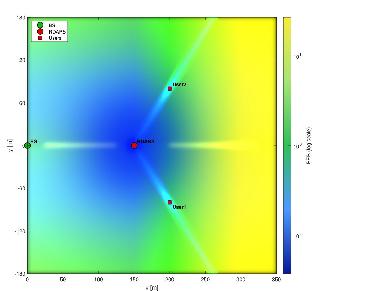
Fig. 6: The PEB for different positions of target, analysing the effect of geometry on ISAC performance.

Fig. 7: The PEB as a function of total number of RDARS elements, for the following structures: passive RIS, DAS and RDARS.

V-A Beampatterns

This section presents the beampattern results for the BS and RDARS, shown in Fig. 3 and Fig. 3. The scenario considers a target at 60∘60^{\circ} azimuth, two users at 10∘10^{\circ} and 20∘20^{\circ} and an RDARS at 45∘45^{\circ}. The RDARS and target are located at a distance of 150 meters from BS. The RDARS phase have been adjusted in a way that four beam configurations are evaluated: reflection beam focused on target, on users, randomly generated and optimally designed. The figures show four distinct peaks near the users, RDARS and target. At user’s locations, the strongest peak corresponds to phase on user, whereas the weakest corresponds to phase on target case. Near the target location, however, this behavior is reversed. The optimal phase produces an intermediate peak between these two extremes. For performance comparison, the PEB is used as an accuracy metric that is equal to the square root of the CRB. Using the calculated FIM, the PEB is defined as follows:

𝒫≜tr⁡(𝐉e−1​(𝐩))=CRB.\mathcal{P}\triangleq\sqrt{\operatorname{tr}\bigl(\mathbf{J}_{e}^{-1}(\mathbf{p})\bigr)}=\sqrt{\operatorname{CRB}}. (61)

Directing the beam closer to the users increases the communication power and improves the SINR performance, albeit at the cost of reduced radar power, leading to higher PEB and less accurate sensing. Conversely, steering the beam toward the target reverses this trade-off. To facilitate comparison across configurations, the corresponding SINR and PEB values are illustrated in Fig. 3. The optimal phase case achieves a balanced PEB of 5.48 m and outperforms other configurations in both metrics. Notably, while the ”phase on target” configuration yields a lower PEB (2.150 m), it fails to meet the desired communication quality, achieving only 21.8 dB SINR compared to 30.9 dB for the optimal design, thereby demonstrating the effectiveness of our framework in balancing sensing and communication under constraints. To provide further engineering insights, we examine several special cases: the SISO case reveals the optimal phase alignment maximizing reflection gain; the single-user case illustrates the distribution gain of connected RDARS elements; the pure LoS scenario highlights the sensitivity of localization accuracy to the BS–RDARS–target geometry; and the high-SNR regime highlights the pronounced mode-selection gain, as the selection of connected elements shapes the FIM eigenvalue structure. Collectively, these simplified cases clarify the roles of reflection, distribution, and mode-selection gains, and offer practical design guidelines.

V-B ISAC Trade-off Analysis

Fig. 5 and Fig. 5 investigate the trade-off between sensing and communication by analyzing the effects of two key parameters on the PEB: the number of users and the minimum SINR threshold γ¯k\overline{\gamma}_{k}. If the number of users or SINR threshold grow, the communication power will increase. As a result, the radar power will decrease. therefore, PEB will increase, which indicates a decrease in localization accuracy. The proposed RDARS framework generalizes two existing architectures: Passive RIS and DAS. These correspond to special cases of RDARS where the number of connected elements is zero or equal to the total number of elements, respectively. Since RDARS inherently combines both reflection and connection capabilities, it offers greater design flexibility and degrees of freedom. Also, due to the reduction in the number of connected elements in RDARS-based systems compared to DAS architecture, the need for costly RF chains is significantly reduced, which represents a very good advantage of RDARS. Consequently, as clearly illustrated in the results, RDARS achieves significantly better performance and a substantially lower PEB compared to passive RIS and DAS.

Fig. 8: The PEB as a function of signal bandwidth.

Fig. 9: The PEB versus number of BS antennas.

Fig. 10: The PEB as a function of transmit power, for the following structures: passive RIS, DAS and RDARS.

Fig. 11: The PEB as a function of number of RDARS connected elements, analysing the selection gain of RDARS in comparison with passive RIS and DAS.

V-C Geometric Analysis

The achievable localization accuracy is evaluated from a geometric perspective, shown in Fig. 7. The scenario consists of a BS at (0,0)(0,0), an RDARS at (150,0)(150,0) m, and two users at (200,±80)(200,\pm 80) m. By varying the target location, the corresponding PEB is computed. The results, illustrated by the color spectrum in the contour plot, reveal several geometric insights. The region between the BS and the RDARS exhibits the lowest PEB, indicating the highest localization accuracy. As the target moves away from this baseline, the PEB gradually increases. A high-error region with low accuracy is observed along the half-line extending from the RDARS location toward infinity. Along this half-line, the circular fixed-delay contours of the direct path are tangential to the elliptical fixed-delay contours of the indirect path, resulting in significantly increased sensitivity to noise in the localization process. Furthermore, along the diagonal paths between the RDARS and the users, the PEB is relatively lower compared to the surrounding regions. This improvement can be attributed to enhanced signal illumination when the target, RDARS and users are approximately aligned. These observations underscore the importance of geometric layout in ISAC system design.

V-D Analysis of System Design Parameters

The final set of simulation results, presented in Figs. 7–11, analyzes key system parameters. As expected from communication-theoretic principles, the PEB consistently decreases with increasing bandwidth, number of BS antennas, total RDARS elements, and transmit power. Notably, even a small number of connected RDARS elements yields a substantially lower PEB compared to passive RIS and DAS, with the lowest PEB achieved at approximately 40 connected elements, although practical and economic constraints render such a large number cost-ineffective. The proposed RDARS framework inherently generalizes all benchmark architectures—passive RIS corresponds to a=0a=0, DAS corresponds to a=Na=N. The results in Figs. 7,  11, and  11 collectively confirm the scalability of the proposed framework to large-scale antenna systems, where the performance gains over passive RIS and DAS remain substantial as the number of BS antennas and RDARS elements increases, while the required number of active RF chains remains remarkably small. This hardware efficiency is particularly advantageous in massive MIMO deployments, where reducing active components is critical for cost and power consumption. These parametric analyses provide valuable practical insights for future RDARS and ISAC system design.

VI Conclusion

This paper investigated a novel RDARS-aided ISAC framework for 6G networks, addressing the joint optimization of the base station’s active beamforming and the RDARS’s dynamic mode selection and passive reflection. The objective was to minimize the CRB for target localization accuracy while satisfying stringent communication quality-of-service constraints defined by user SINR thresholds. To tackle this challenging non-convex mixed-integer problem, we developed an efficient iterative algorithm based on the AO framework, effectively integrating MM and Penalty techniques. Extensive simulations demonstrated the superiority of the proposed design. By analyzing various beampatterns, system geometries and performance trade-offs, the results conclusively showed that the dynamically configured RDARS achieves a significantly lower PEB for a given SINR requirement compared to conventional passive RIS and DAS benchmarks. This superior performance stems from the synergistic exploitation of reflection, distribution and mode-selection gains unique to the RDARS architecture. Future research directions include extending this framework to multi-target localization scenarios, investigating RDARS-aided ISAC under imperfect channel state information, extending the model to multi-user localization downlink scenarios without ISAC, exploring the integration of RDARS with advanced waveform design for enhanced spectral efficiency, and extending the proposed framework to account for random and dynamic RCS fluctuations using Bayesian or modified Cramér–Rao bounds. Furthermore, a comprehensive investigation of multiple RDARS panels—encompassing optimal placement, inter-panel interference characterization, and trade-offs between the number of panels and the number of elements per panel—remains a compelling avenue for future work, as the present study establishes the foundational single-panel CRB-based optimization as a necessary first step toward such complex deployments.

Appendix A Calculation of the FIM

Based on the complex Gaussian distribution of the received signal in (6), the elements of 𝐉𝜼\mathbf{J}_{\bm{\eta}} are given by [43]:

𝐉𝜼\displaystyle\mathbf{J}_{\bm{\eta}} =[𝐉𝝉,𝝉𝐉𝝉,𝜽𝐉𝝉,𝜶𝐉𝜽,𝝉𝐉𝜽,𝜽𝐉𝜽,𝜶𝐉𝜶,𝝉𝐉𝜶,𝜽𝐉𝜶,𝜶],\displaystyle=\scalebox{0.9}{$\begin{bmatrix}\mathbf{J}_{\bm{\tau},\bm{\tau}}&\mathbf{J}_{\bm{\tau},\bm{\theta}}&\mathbf{J}_{\bm{\tau},\bm{\alpha}}\\ \mathbf{J}_{\bm{\theta},\bm{\tau}}&\mathbf{J}_{\bm{\theta},\bm{\theta}}&\mathbf{J}_{\bm{\theta},\bm{\alpha}}\\ \mathbf{J}_{\bm{\alpha},\bm{\tau}}&\mathbf{J}_{\bm{\alpha},\bm{\theta}}&\mathbf{J}_{\bm{\alpha},\bm{\alpha}}\end{bmatrix}$}, (62)
𝐉𝜼(i,j)\displaystyle\mathbf{J}^{(\textit{i},\textit{j})}_{\bm{\eta}} =2σ2​∑n=−Ns−12Ns−12ℜ⁡{∂𝝁H​[n]∂ηi,j​∂𝝁⁡[n]∂ηi,j}.\displaystyle=\scalebox{0.9}{$\frac{2}{\sigma^{2}}\sum_{n=-\frac{N_{s}-1}{2}}^{\frac{N_{s}-1}{2}}\Re\left\{\frac{\partial\bm{\mu}^{H}[n]}{\partial\eta_{i,j}}\frac{\partial\bm{\mu}[n]}{\partial\eta_{i,j}}\right\}$}. (63)

The FIM elements are derived from the partial derivatives of the signal model. The derivatives with respect to delays τi\tau_{i} are:

∂𝝁⁡[n]∂τ1\displaystyle\frac{\partial\bm{\mu}[n]}{\partial\tau_{1}} =[α1​e−j​2​π​n​Δ​f​τ1​[𝐆1,0]​𝐗​[n]​(−j​2​π​n​Δ​f)𝟎],\displaystyle=\scalebox{0.9}{$\begin{bmatrix}\alpha_{1}e^{-j2\pi n\Delta f\tau_{1}}[\mathbf{G}_{1},0]\mathbf{X}[n](-j2\pi n\Delta f)\\ \bm{0}\end{bmatrix}$}, (64)
∂𝝁⁡[n]∂τ2\displaystyle\frac{\partial\bm{\mu}[n]}{\partial\tau_{2}} =[𝟎α2​e−j​2​π​n​Δ​f​τ2​[𝐆2,0]​𝐗​[n]​(−j​2​π​n​Δ​f)],\displaystyle=\scalebox{0.9}{$\begin{bmatrix}\bm{0}\\ \alpha_{2}e^{-j2\pi n\Delta f\tau_{2}}[\mathbf{G}_{2},0]\mathbf{X}[n](-j2\pi n\Delta f)\end{bmatrix}$}, (65)

Analogous expressions can be derived for τ3\tau_{3}, τ4\tau_{4} and τ5\tau_{5}. The derivatives with respect to delays angles θi\theta_{i} and path losses αi\alpha_{i} are given by:

∂𝝁⁡[n]∂θ1\displaystyle\frac{\partial\bm{\mu}[n]}{\partial\theta_{1}} =[α1​e−j​2​π​n​Δ​f​τ1​[𝐆˙1,0]​𝐗​[n]+α3​e−j​2​π​n​Δ​f​τ3​[𝐆˙3,0]​𝐗​[n]+α5​e−j​2​π​n​Δ​f​τ5​[0,𝐆˙5]​𝐗​[n]α2​e−j​2​π​n​Δ​f​τ2​[𝐆˙2,0]​𝐗​[n]],\displaystyle=\scalebox{0.85}{$\begin{bmatrix}\alpha_{1}e^{-j2\pi n\Delta f\tau_{1}}[\dot{\mathbf{G}}_{1},0]\mathbf{X}[n]\\ +\alpha_{3}e^{-j2\pi n\Delta f\tau_{3}}[\dot{\mathbf{G}}_{3},0]\mathbf{X}[n]\\ +\alpha_{5}e^{-j2\pi n\Delta f\tau_{5}}[0,\dot{\mathbf{G}}_{5}]\mathbf{X}[n]\\ \alpha_{2}e^{-j2\pi n\Delta f\tau_{2}}[\dot{\mathbf{G}}_{2},0]\mathbf{X}[n]\end{bmatrix}$}, (66)
∂𝝁⁡[n]∂θ2\displaystyle\frac{\partial\bm{\mu}[n]}{\partial\theta_{2}} =[α3​e−j​2​π​n​Δ​f​τ3​[𝐆˙3,θ2,0]​𝐗​[n]+α5​e−j​2​π​n​Δ​f​τ5​[0,𝐆˙5,θ2]​𝐗​[n]α2​e−j​2​π​n​Δ​f​τ2​[𝐆˙2,θ2,0]​𝐗​[n]+α4​e−j​2​π​n​Δ​f​τ4​[0,𝐆˙4,θ2]​𝐗​[n]],\displaystyle=\scalebox{0.82}{$\begin{bmatrix}\alpha_{3}e^{-j2\pi n\Delta f\tau_{3}}[\dot{\mathbf{G}}_{3,\theta_{2}},0]\mathbf{X}[n]+\alpha_{5}e^{-j2\pi n\Delta f\tau_{5}}[0,\dot{\mathbf{G}}_{5,\theta_{2}}]\mathbf{X}[n]\\ \alpha_{2}e^{-j2\pi n\Delta f\tau_{2}}[\dot{\mathbf{G}}_{2,\theta_{2}},0]\mathbf{X}[n]+\alpha_{4}e^{-j2\pi n\Delta f\tau_{4}}[0,\dot{\mathbf{G}}_{4,\theta_{2}}]\mathbf{X}[n]\end{bmatrix}$}, (67)
∂𝝁⁡[n]∂αiR\displaystyle\frac{\partial\bm{\mu}[n]}{\partial\alpha_{i}^{R}} =−j​∂𝝁⁡[n]∂αiI=[e−j​2​π​n​Δ​f​τi​[𝐆i,0]​𝐗​[n]𝟎].\displaystyle=-j\frac{\partial\bm{\mu}[n]}{\partial\alpha_{i}^{I}}=\scalebox{0.86}{$\begin{bmatrix}e^{-j2\pi n\Delta f\tau_{i}}[\mathbf{G}_{i},0]\mathbf{X}[n]\\ \bm{0}\end{bmatrix}$}. (68)

Under the resolvable-path/score-orthogonality approximation stated in Section III, the FIM reduces to 𝐉𝜼=blkdiag⁡[𝐉τ,𝐉θ,𝐉α]\mathbf{J}_{\bm{\eta}}=\operatorname{blkdiag}[\mathbf{J}_{\tau},\mathbf{J}_{\theta},\mathbf{J}_{\alpha}]. By substituting the partial derivatives (64)-(68) into the Slepian-Bangs (63), the diagonal elements of the FIM are obtained as (16)-(21).

The transformation matrix 𝐓\mathbf{T} is defined as the Jacobian of 𝜼\bm{\eta} with respect to 𝜸\bm{\gamma} and can be obtained as:

𝐓≜∂η∂γ=[𝚵𝐎𝐎𝐈10],\mathbf{T}\triangleq\frac{\partial\eta}{\partial\gamma}=\begin{bmatrix}\bm{\Xi}&\mathbf{O}\\ \mathbf{O}&\mathbf{I}_{10}\end{bmatrix}, (69)

where 𝚵=[∇𝝉,𝐩T,∇𝜽,𝐩T]T\bm{\Xi}=[{\nabla}_{\bm{\tau},\mathbf{p}}^{T},{\nabla}_{\bm{\theta},\mathbf{p}}^{T}]^{T}. Considering the five paths introduced in (6) and definition of the parameters 𝐞1=(𝐩−𝐪)T‖𝐩−𝐪‖,𝐞2=(𝐩−𝐫)T‖𝐩−𝐫‖\mathbf{e}_{1}=\frac{(\mathbf{p}-\mathbf{q})^{T}}{\|\mathbf{p}-\mathbf{q}\|},\quad\mathbf{e}_{2}=\frac{(\mathbf{p}-\mathbf{r})^{T}}{\|\mathbf{p}-\mathbf{r}\|}, the gradient expressions with respect to the position 𝐩\mathbf{p} are given by:

∇τ1,p\displaystyle\nabla_{\tau_{1},p} =2c​𝐞1,\displaystyle=\scalebox{0.9}{$\frac{2}{c}\mathbf{e}_{1}$}, (70)
∇τ2,p\displaystyle\nabla_{\tau_{2},p} =∇τ3,p=∇τ5,p=1c​[𝐞1+𝐞2],\displaystyle=\nabla_{\tau_{3},p}=\nabla_{\tau_{5},p}=\scalebox{0.9}{$\frac{1}{c}[\mathbf{e}_{1}+\mathbf{e}_{2}]$}, (71)
∇τ4,p\displaystyle\nabla_{\tau_{4},p} =2c​𝐞2.\displaystyle=\scalebox{0.9}{$\frac{2}{c}\mathbf{e}_{2}$}. (72)

where parameter cc denotes the speed of light in vacuum. The angles θ1\theta_{1} and θ2\theta_{2} are computed as: θ1=tan−1⁡(yp−yqxp−xq)\theta_{1}=\tan^{-1}\left(\frac{y_{p}-y_{q}}{x_{p}-x_{q}}\right) and θ2=tan−1⁡(yp−yrxp−xr)\theta_{2}=\tan^{-1}\left(\frac{y_{p}-y_{r}}{x_{p}-x_{r}}\right). Thus, the gradient vectors are given by:

∇θ1,𝐩=[yq−yp(xp−xq)2+(yp−yq)2,xp−xq(xp−xq)2+(yp−yq)2]=1‖𝐩−𝐪‖​[−sin⁡θ1,cos⁡θ1]=𝝆1T,\displaystyle\begin{split}\nabla_{\theta_{1},\mathbf{p}}&=\scalebox{0.9}{$\left[\frac{y_{q}-y_{p}}{(x_{p}-x_{q})^{2}+(y_{p}-y_{q})^{2}},\frac{x_{p}-x_{q}}{(x_{p}-x_{q})^{2}+(y_{p}-y_{q})^{2}}\right]$}\\ &=\scalebox{0.9}{$\frac{1}{\|\mathbf{p}-\mathbf{q}\|}\left[-\sin\theta_{1},\cos\theta_{1}\right]$}=\scalebox{0.9}{$\bm{\rho}_{1}^{T}$},\end{split} (73)
∇θ2,𝐩=1‖𝐫−𝐩‖​[−sin⁡θ2,cos⁡θ2]=𝝆2T.\displaystyle\begin{split}\nabla_{\theta_{2},\mathbf{p}}&=\scalebox{0.9}{$\frac{1}{\|\mathbf{r}-\mathbf{p}\|}\left[-\sin\theta_{2},\cos\theta_{2}\right]$}=\scalebox{0.9}{$\bm{\rho}_{2}^{T}$}.\end{split} (74)

Therefore, the FIM for 𝜸\bm{\gamma} is given by:

𝐉𝜸=𝐓T​𝐉𝜼​𝐓=[𝚵𝐎𝐎𝐈]T​𝐉𝜼​[𝚵𝐎𝐎𝐈]=[𝚵T​𝐉m​𝚵𝐎𝐎𝐉𝜶],\mathbf{J}_{\bm{\gamma}}=\mathbf{T}^{T}\,\mathbf{J}_{\bm{\eta}}\,\mathbf{T}=\scalebox{0.9}{$\begin{bmatrix}\bm{\Xi}&\mathbf{O}\\ \mathbf{O}&\mathbf{I}\end{bmatrix}^{T}\mathbf{J}_{\bm{\eta}}\begin{bmatrix}\bm{\Xi}&\mathbf{O}\\ \mathbf{O}&\mathbf{I}\end{bmatrix}$}=\scalebox{0.9}{$\begin{bmatrix}\bm{\Xi}^{T}\mathbf{J}_{m}\bm{\Xi}&\mathbf{O}\\ \mathbf{O}&\mathbf{J}_{\bm{\alpha}}\end{bmatrix}$}, (75)

where 𝐉𝒎=blkdiag⁡[𝐉τ,𝐉θ]\mathbf{J}_{\bm{m}}=\operatorname{blkdiag}[\mathbf{J}_{\tau},\mathbf{J}_{\theta}]. We can also obtain:

𝚵\displaystyle\bm{\Xi} =[2c−1𝐞1,c−1𝐞1+c−1𝐞2,c−1𝐞1+c−1𝐞2,\displaystyle=\scalebox{0.9}{$\left[2c^{-1}\mathbf{e}_{1},c^{-1}\mathbf{e}_{1}+c^{-1}\mathbf{e}_{2},c^{-1}\mathbf{e}_{1}+c^{-1}\mathbf{e}_{2},\right.$}
2c−1𝐞2,c−1𝐞1+c−1𝐞2,𝝆1,𝝆2]T.\displaystyle\quad\scalebox{0.9}{$\left.2c^{-1}\mathbf{e}_{2},c^{-1}\mathbf{e}_{1}+c^{-1}\mathbf{e}_{2},\bm{\rho}_{1},\bm{\rho}_{2}\right]^{T}$}. (76)

Therefore, the position-related submatrix denoted as effective FIM is derived as follows:

𝐉e2×2\displaystyle\mathbf{J}_{e_{2\times 2}} =𝚵T​𝐉m​𝚵\displaystyle=\bm{\Xi}^{T}\mathbf{J}_{m}\bm{\Xi}
=Jτ1​τ1​4c2​𝐞1​𝐞1T+Jτ2​τ2​1c2​[𝐞1+𝐞2]​[𝐞1+𝐞2]T\displaystyle=\scalebox{0.9}{$J_{\tau_{1}\tau_{1}}\frac{4}{c^{2}}\mathbf{e}_{1}\mathbf{e}_{1}^{T}+J_{\tau_{2}\tau_{2}}\frac{1}{c^{2}}[\mathbf{e}_{1}+\mathbf{e}_{2}][\mathbf{e}_{1}+\mathbf{e}_{2}]^{T}$}
 

+Jτ3​τ3​1c2​[𝐞1+𝐞2]​[𝐞1+𝐞2]T+Jτ4​τ4​4c2​𝐞2​𝐞2T+J_{\tau_{3}\tau_{3}}\frac{1}{c^{2}}[\mathbf{e}_{1}+\mathbf{e}_{2}][\mathbf{e}_{1}+\mathbf{e}_{2}]^{T}+J_{\tau_{4}\tau_{4}}\frac{4}{c^{2}}\mathbf{e}_{2}\mathbf{e}_{2}^{T}


+Jτ5​τ5​1c2​[𝐞1+𝐞2]​[𝐞1+𝐞2]T+J_{\tau_{5}\tau_{5}}\frac{1}{c^{2}}[\mathbf{e}_{1}+\mathbf{e}_{2}][\mathbf{e}_{1}+\mathbf{e}_{2}]^{T}

+Jθ1​θ1​𝝆1​𝝆1T+Jθ2​θ2​𝝆2​𝝆2T.\displaystyle\quad\scalebox{0.9}{$+J_{\theta_{1}\theta_{1}}\bm{\rho}_{1}\bm{\rho}_{1}^{T}+J_{\theta_{2}\theta_{2}}\bm{\rho}_{2}\bm{\rho}_{2}^{T}$}. (77)

Substituting the individual FIM elements, we can obtain:

𝐉e\displaystyle\mathbf{J}_{e} =2​Ns​(Ns2−1)12​σ2​c2​(2​π​Δ​f)2×\displaystyle=\scalebox{0.9}{$\frac{2N_{s}(N_{s}^{2}-1)}{12\sigma^{2}c^{2}}(2\pi\Delta f)^{2}$}\times
 

[|α1|2tr(𝐆1𝐑X​1𝐆1H)4𝐞1𝐞1T\Bigg[|\alpha_{1}|^{2}\mathrm{tr}(\mathbf{G}_{1}\mathbf{R}_{X1}\mathbf{G}_{1}^{H})4\mathbf{e}_{1}\mathbf{e}_{1}^{T}


+|α2|2​tr​(𝐆2​𝐑X​1​𝐆2H)​(𝐞1+𝐞2)​(𝐞1+𝐞2)T+|\alpha_{2}|^{2}\mathrm{tr}(\mathbf{G}_{2}\mathbf{R}_{X1}\mathbf{G}_{2}^{H})(\mathbf{e}_{1}+\mathbf{e}_{2})(\mathbf{e}_{1}+\mathbf{e}_{2})^{T}


+|α3|2​tr​(𝐆3​𝐑X​1​𝐆3H)​(𝐞1+𝐞2)​(𝐞1+𝐞2)T+|\alpha_{3}|^{2}\mathrm{tr}(\mathbf{G}_{3}\mathbf{R}_{X1}\mathbf{G}_{3}^{H})(\mathbf{e}_{1}+\mathbf{e}_{2})(\mathbf{e}_{1}+\mathbf{e}_{2})^{T}


+4​|α4|2​tr​(𝐆4​𝐑X​2​𝐆4H)​𝐞2​𝐞2T+4|\alpha_{4}|^{2}\mathrm{tr}(\mathbf{G}_{4}\mathbf{R}_{X2}\mathbf{G}_{4}^{H})\mathbf{e}_{2}\mathbf{e}_{2}^{T}


+|α5|2tr(𝐆5𝐑X​2𝐆5H)(𝐞1+𝐞2)(𝐞1+𝐞2)T]+|\alpha_{5}|^{2}\mathrm{tr}(\mathbf{G}_{5}\mathbf{R}_{X2}\mathbf{G}_{5}^{H})(\mathbf{e}_{1}+\mathbf{e}_{2})(\mathbf{e}_{1}+\mathbf{e}_{2})^{T}\Bigg]

+[2σ2|α1|2tr{𝐆˙1,θ1𝐑X​1𝐆˙1,θ1H}Ns\displaystyle\quad+\scalebox{0.9}{$\Bigg[\frac{2}{\sigma^{2}}|\alpha_{1}|^{2}\mathrm{tr}\{\dot{\mathbf{G}}_{1,\theta_{1}}\mathbf{R}_{X1}\dot{\mathbf{G}}_{1,\theta_{1}}^{H}\}N_{s}$}
 

+2σ2​|α3|2​tr​{𝐆˙3,θ1​𝐑X​1​𝐆˙3,θ1H}​Ns+\frac{2}{\sigma^{2}}|\alpha_{3}|^{2}\mathrm{tr}\{\dot{\mathbf{G}}_{3,\theta_{1}}\mathbf{R}_{X1}\dot{\mathbf{G}}_{3,\theta_{1}}^{H}\}N_{s}


+2σ2​|α5|2​tr​{𝐆˙5,θ1​𝐑X​2​𝐆˙5,θ1H}​Ns+\frac{2}{\sigma^{2}}|\alpha_{5}|^{2}\mathrm{tr}\{\dot{\mathbf{G}}_{5,\theta_{1}}\mathbf{R}_{X2}\dot{\mathbf{G}}_{5,\theta_{1}}^{H}\}N_{s}


+2σ2|α2|2tr{𝐆˙2,θ1𝐑X​1𝐆˙2,θ1H}Ns]𝝆1𝝆1T+\frac{2}{\sigma^{2}}|\alpha_{2}|^{2}\mathrm{tr}\{\dot{\mathbf{G}}_{2,\theta_{1}}\mathbf{R}_{X1}\dot{\mathbf{G}}_{2,\theta_{1}}^{H}\}N_{s}\Bigg]\bm{\rho}_{1}\bm{\rho}_{1}^{T}

+[2σ2|α5|2tr{𝐆˙5,θ2𝐑X​2𝐆˙5,θ2H}Ns\displaystyle\quad+\scalebox{0.9}{$\Bigg[\frac{2}{\sigma^{2}}|\alpha_{5}|^{2}\mathrm{tr}\{\dot{\mathbf{G}}_{5,\theta_{2}}\mathbf{R}_{X2}\dot{\mathbf{G}}_{5,\theta_{2}}^{H}\}N_{s}$}
 

+2σ2​|α2|2​tr​{𝐆˙2,θ2​𝐑X​1​𝐆˙2,θ2H}​Ns+\frac{2}{\sigma^{2}}|\alpha_{2}|^{2}\mathrm{tr}\{\dot{\mathbf{G}}_{2,\theta_{2}}\mathbf{R}_{X1}\dot{\mathbf{G}}_{2,\theta_{2}}^{H}\}N_{s}


+2σ2​|α3|2​tr​{𝐆˙3,θ2​𝐑X​1​𝐆˙3,θ2H}​Ns+\frac{2}{\sigma^{2}}|\alpha_{3}|^{2}\mathrm{tr}\{\dot{\mathbf{G}}_{3,\theta_{2}}\mathbf{R}_{X1}\dot{\mathbf{G}}_{3,\theta_{2}}^{H}\}N_{s}

+2σ2|α4|2tr{𝐆˙4,θ2𝐑X​2𝐆˙4,θ2H}Ns]𝝆2𝝆2T.\displaystyle\quad\scalebox{0.9}{$+\frac{2}{\sigma^{2}}|\alpha_{4}|^{2}\mathrm{tr}\{\dot{\mathbf{G}}_{4,\theta_{2}}\mathbf{R}_{X2}\dot{\mathbf{G}}_{4,\theta_{2}}^{H}\}N_{s}\Bigg]\bm{\rho}_{2}\bm{\rho}_{2}^{T}$}. (78a)

Then, we define new parameters as follows:

λk\displaystyle\lambda_{k} ≜2​π2​Ns​(Ns2−1)​(Δ​f)23​σ2​c2​|αk|2​lk,k=1,2,…,5\displaystyle\triangleq\scalebox{0.9}{$\frac{2\pi^{2}N_{s}(N_{s}^{2}-1)(\Delta f)^{2}}{3\sigma^{2}c^{2}}|\alpha_{k}|^{2}l_{k}$},\qquad\scalebox{0.9}{$k=1,2,\ldots,5$} (79)

where l1=4​tr⁡{𝐆1​𝐑x​1​𝐆1H}l_{1}=4\operatorname{tr}\{\mathbf{G}_{1}\mathbf{R}_{x1}\mathbf{G}_{1}^{H}\}, l2=tr⁡{𝐆2​𝐑x​1​𝐆2H}l_{2}=\operatorname{tr}\{\mathbf{G}_{2}\mathbf{R}_{x1}\mathbf{G}_{2}^{H}\}, l3=tr⁡{𝐆3​𝐑x​1​𝐆3H}l_{3}=\operatorname{tr}\{\mathbf{G}_{3}\mathbf{R}_{x1}\mathbf{G}_{3}^{H}\}, l4=4​tr⁡{𝐆4​𝐑x​2​𝐆4H}l_{4}=4\operatorname{tr}\{\mathbf{G}_{4}\mathbf{R}_{x2}\mathbf{G}_{4}^{H}\} and l5=tr⁡{𝐆5​𝐑x​2​𝐆5H}l_{5}=\operatorname{tr}\{\mathbf{G}_{5}\mathbf{R}_{x2}\mathbf{G}_{5}^{H}\}.

δk\displaystyle\delta_{k} ≜2σ2​Ns​|αk|2​mk,k=1,2,3,5.\displaystyle\triangleq\scalebox{0.9}{$\frac{2}{\sigma^{2}}N_{s}|\alpha_{k}|^{2}m_{k}$},\quad\scalebox{0.9}{$k=1,2,3,5$}. (80)

where mk=tr⁡{𝐆˙k,θ1​𝐑x(k)​𝐆˙k,θ1H}m_{k}=\operatorname{tr}\{\dot{\mathbf{G}}_{k,\theta_{1}}\mathbf{R}_{x}^{(k)}\dot{\mathbf{G}}_{k,\theta_{1}}^{H}\}, with 𝐑x(k)=𝐑x​1\mathbf{R}_{x}^{(k)}=\mathbf{R}_{x1} for k∈{1,2,3}k\in\{1,2,3\} and 𝐑x(k)=𝐑x​2\mathbf{R}_{x}^{(k)}=\mathbf{R}_{x2} for k=5k=5.

ηk\displaystyle\eta_{k} ≜2σ2​Ns​|αk|2​nk,k=2,3,4,5\displaystyle\triangleq\scalebox{0.9}{$\frac{2}{\sigma^{2}}N_{s}|\alpha_{k}|^{2}n_{k}$},\quad\scalebox{0.9}{$k=2,3,4,5$} (81)

where n2=tr⁡{𝐆˙2,θ2​𝐑x​1​𝐆˙2,θ2H},n_{2}=\mathrm{tr}\{\dot{\mathbf{G}}_{2,\theta_{2}}\mathbf{R}_{x1}\dot{\mathbf{G}}_{2,\theta_{2}}^{H}\}, n3=tr⁡{𝐆˙3,θ2​𝐑x​1​𝐆˙3,θ2H},n_{3}=\mathrm{tr}\{\dot{\mathbf{G}}_{3,\theta_{2}}\mathbf{R}_{x1}\dot{\mathbf{G}}_{3,\theta_{2}}^{H}\}, n4=tr⁡{𝐆˙4,θ2​𝐑x​2​𝐆˙4,θ2H}n_{4}=\mathrm{tr}\{\dot{\mathbf{G}}_{4,\theta_{2}}\mathbf{R}_{x2}\dot{\mathbf{G}}_{4,\theta_{2}}^{H}\} and n5=tr⁡{𝐆˙5,θ2​𝐑x​2​𝐆˙5,θ2H}n_{5}=\mathrm{tr}\{\dot{\mathbf{G}}_{5,\theta_{2}}\mathbf{R}_{x2}\dot{\mathbf{G}}_{5,\theta_{2}}^{H}\}. Thus, the equivalent FIM is:

𝐉e\displaystyle\mathbf{J}_{e} =(λ1+λ2+λ3+λ5)​𝐞1​𝐞1T\displaystyle=\scalebox{0.9}{$(\lambda_{1}+\lambda_{2}+\lambda_{3}+\lambda_{5})\mathbf{e}_{1}\mathbf{e}_{1}^{T}$}
 

+(λ2+λ3+λ4+λ5)​𝐞2​𝐞2T+(\lambda_{2}+\lambda_{3}+\lambda_{4}+\lambda_{5})\,\mathbf{e}_{2}\mathbf{e}_{2}^{T}


+(λ2+λ3+λ5)​𝐞1​𝐞2T+(λ2+λ3+λ5)​𝐞2​𝐞1T+(\lambda_{2}+\lambda_{3}+\lambda_{5})\,\mathbf{e}_{1}\mathbf{e}_{2}^{T}+(\lambda_{2}+\lambda_{3}+\lambda_{5})\,\mathbf{e}_{2}\mathbf{e}_{1}^{T}

+(δ1+δ2+δ3+δ5)​𝝆1​𝝆1T+(η2+η3+η4+η5)​𝝆2​𝝆2T.\displaystyle\quad\scalebox{0.9}{$+(\delta_{1}+\delta_{2}+\delta_{3}+\delta_{5})\,\bm{\rho}_{1}\bm{\rho}_{1}^{T}+(\eta_{2}+\eta_{3}+\eta_{4}+\eta_{5})\,\bm{\rho}_{2}\bm{\rho}_{2}^{T}$}. (82)

Then, we use additional scalar factor as follows: Li≜2​π2​Ns​(Ns2−1)3​σ2​c2​(Δ​f)2​|αi|2L_{i}\triangleq\scalebox{0.9}{$\frac{2\pi^{2}N_{s}(N_{s}^{2}-1)}{3\sigma^{2}c^{2}}(\Delta f)^{2}|\alpha_{i}|^{2}$} and 𝐌i≜𝐆iH​𝐆i\mathbf{M}_{i}\triangleq\mathbf{G}_{i}^{H}\mathbf{G}_{i}. Thus, we can obtain:

λ1\displaystyle\lambda_{1} =8​π2​Ns​(Ns2−1)3​σ2​c2​(Δ​f)2​|α1|2​tr​{𝐆1​𝐑x​1​𝐆1H}\displaystyle=\scalebox{0.9}{$\frac{8\pi^{2}N_{s}(N_{s}^{2}-1)}{3\sigma^{2}c^{2}}(\Delta f)^{2}|\alpha_{1}|^{2}\mathrm{tr}\{\mathbf{G}_{1}\mathbf{R}_{x1}\mathbf{G}_{1}^{H}\}$}
=4​L1​tr​{𝐌1​𝐑x​1},\displaystyle=\scalebox{0.9}{$4L_{1}\,\mathrm{tr}\{\mathbf{M}_{1}\mathbf{R}_{x1}\}$}, (83)

Analogous expressions can be derived λ2=L2​tr​{𝐌2​𝐑X​1},\lambda_{2}=L_{2}\mathrm{tr}\{\mathbf{M}_{2}\mathbf{R}_{X1}\}, λ3=L3​tr​{𝐌3​𝐑X​1},\lambda_{3}=L_{3}\mathrm{tr}\{\mathbf{M}_{3}\mathbf{R}_{X1}\}, λ4=4​L4​tr​{𝐌4​𝐑X​2}\lambda_{4}=4L_{4}\mathrm{tr}\{\mathbf{M}_{4}\mathbf{R}_{X2}\} and λ5=L5​tr​{𝐌5​𝐑X​2}\lambda_{5}=L_{5}\mathrm{tr}\{\mathbf{M}_{5}\mathbf{R}_{X2}\}. Thus the equivalent FIM is:

𝐉e\displaystyle\mathbf{J}_{e} =[J1,1J1,2J1,2J2,2]=𝚵T​𝐉m​𝚵\displaystyle=\begin{bmatrix}J_{1,1}&J_{1,2}\\ J_{1,2}&J_{2,2}\end{bmatrix}=\bm{\Xi}^{T}\mathbf{J}_{m}\bm{\Xi}
=(4​L1​tr⁡{𝐌1​𝐑x​1}+L2​tr⁡{𝐌2​𝐑x​1}CLOSE+L3​tr⁡{𝐌3​𝐑x​1}\displaystyle=\scalebox{0.9}{$\big(4L_{1}\operatorname{tr}\{\mathbf{M}_{1}\mathbf{R}_{x1}\}+L_{2}\operatorname{tr}\{\mathbf{M}_{2}\mathbf{R}_{x1}\}$}+L_{3}\operatorname{tr}\{\mathbf{M}_{3}\mathbf{R}_{x1}\}
 

OPEN+4​L4​tr⁡{𝐌4​𝐑x​2}+L5​tr⁡{𝐌5​𝐑x​2})​𝐞1​𝐞1T+4L_{4}\operatorname{tr}\{\mathbf{M}_{4}\mathbf{R}_{x2}\}+L_{5}\operatorname{tr}\{\mathbf{M}_{5}\mathbf{R}_{x2}\}\big)\mathbf{e}_{1}\mathbf{e}_{1}^{T}

+(L2​tr⁡{𝐌2​𝐑x​1}+L3​tr⁡{𝐌3​𝐑x​1}CLOSE\displaystyle\quad+\scalebox{0.9}{$\big(L_{2}\operatorname{tr}\{\mathbf{M}_{2}\mathbf{R}_{x1}\}+L_{3}\operatorname{tr}\{\mathbf{M}_{3}\mathbf{R}_{x1}\}$}
OPEN+4​L4​tr⁡{𝐌4​𝐑x​2}+L5​tr⁡{𝐌5​𝐑x​2})​𝐞2​𝐞2T+…\displaystyle\quad\scalebox{0.9}{$+4L_{4}\operatorname{tr}\{\mathbf{M}_{4}\mathbf{R}_{x2}\}+L_{5}\operatorname{tr}\{\mathbf{M}_{5}\mathbf{R}_{x2}\}\big)\mathbf{e}_{2}\mathbf{e}_{2}^{T}$}+\ldots (84)

After collecting the coefficients of the feasible covariance vector 𝐫=[𝐫1T,𝐫2T]T\mathbf{r}=[\mathbf{r}_{1}^{T},\mathbf{r}_{2}^{T}]^{T}, each real EFIM entry is linear in 𝐫\mathbf{r}. Hence, there exist coefficient vectors 𝐜11\mathbf{c}_{11}, 𝐜22\mathbf{c}_{22}, and 𝐜12\mathbf{c}_{12} such that

J11=𝐜11H​𝐫,J22=𝐜22H​𝐫,J12=𝐜12H​𝐫,J_{11}=\mathbf{c}_{11}^{H}\mathbf{r},\qquad J_{22}=\mathbf{c}_{22}^{H}\mathbf{r},\qquad J_{12}=\mathbf{c}_{12}^{H}\mathbf{r}, (85)

with real values on the feasible Hermitian covariance set. The coefficient vectors contain the contributions of both 𝐫1\mathbf{r}_{1} and 𝐫2\mathbf{r}_{2}. Defining

𝐦≜𝐜11+𝐜222,𝐁~≜𝐜11​𝐜22H+𝐜22​𝐜11H2−𝐜12​𝐜12H,\mathbf{m}\triangleq\frac{\mathbf{c}_{11}+\mathbf{c}_{22}}{2},\qquad\widetilde{\mathbf{B}}\triangleq\frac{\mathbf{c}_{11}\mathbf{c}_{22}^{H}+\mathbf{c}_{22}\mathbf{c}_{11}^{H}}{2}-\mathbf{c}_{12}\mathbf{c}_{12}^{H}, (86)

we obtain

CRB=J11+J22J11​J22−J122=𝐫H​𝐦+𝐦H​𝐫𝐫H​𝐁~​𝐫.\operatorname{CRB}=\frac{J_{11}+J_{22}}{J_{11}J_{22}-J_{12}^{2}}=\frac{\mathbf{r}^{H}\mathbf{m}+\mathbf{m}^{H}\mathbf{r}}{\mathbf{r}^{H}\widetilde{\mathbf{B}}\mathbf{r}}. (87)

The off-diagonal blocks of 𝐁~\widetilde{\mathbf{B}} explicitly generate the 𝐫1\mathbf{r}_{1}–𝐫2\mathbf{r}_{2} cross terms. No positive-semidefiniteness of 𝐁~\widetilde{\mathbf{B}} is assumed, which motivates the spectral split used in Section IV-B.

Appendix B Calculation of the CRB in terms of ϕ\phi

For fixed 𝐀\mathbf{A} and 𝐀a\mathbf{A}_{a}, the phase vector affects the radar FIM through Path 3. Define

𝐝0\displaystyle\mathbf{d}_{0} ≜𝐜⁡(θ4)¯⊙(𝐈−𝐀)​𝐜​(θ5),\displaystyle\triangleq\overline{\mathbf{c}(\theta_{4})}\odot(\mathbf{I}-\mathbf{A})\mathbf{c}(\theta_{5}), (88)
𝐝1\displaystyle\mathbf{d}_{1} ≜𝐜⁡(θ4)¯⊙(𝐈−𝐀)​𝐜˙​(θ5),\displaystyle\triangleq\overline{\mathbf{c}(\theta_{4})}\odot(\mathbf{I}-\mathbf{A})\dot{\mathbf{c}}(\theta_{5}), (89)

where 𝐜˙​(θ5)=∂𝐜⁡(θ5)/∂θ2\dot{\mathbf{c}}(\theta_{5})=\partial\mathbf{c}(\theta_{5})/\partial\theta_{2} and ∂θ5/∂θ2=1\partial\theta_{5}/\partial\theta_{2}=1. From (11),

g=𝐝0T​ϕ,∂g∂θ2=𝐝1T​ϕ.g=\mathbf{d}_{0}^{T}\bm{\phi},\qquad\frac{\partial g}{\partial\theta_{2}}=\mathbf{d}_{1}^{T}\bm{\phi}. (90)

Hence

S0​(ϕ)=|g|2=ϕH​𝐐0​ϕ,S1​(ϕ)=|∂g∂θ2|2=ϕH​𝐐1​ϕ,S_{0}(\bm{\phi})=|g|^{2}=\bm{\phi}^{H}\mathbf{Q}_{0}\bm{\phi},\qquad S_{1}(\bm{\phi})=\left|\frac{\partial g}{\partial\theta_{2}}\right|^{2}=\bm{\phi}^{H}\mathbf{Q}_{1}\bm{\phi}, (91)

where 𝐐0=𝐝0∗​𝐝0T\mathbf{Q}_{0}=\mathbf{d}_{0}^{*}\mathbf{d}_{0}^{T} and 𝐐1=𝐝1∗​𝐝1T\mathbf{Q}_{1}=\mathbf{d}_{1}^{*}\mathbf{d}_{1}^{T}. The Path-3 delay information and its θ1\theta_{1} contribution are affine in S0S_{0}, whereas the Path-3 contribution to the θ2\theta_{2} information is affine in S1S_{1}. Consequently, the position-EFIM entries can be written as

Ji​j​(ϕ)=βi​j(0)​S0​(ϕ)+βi​j(1)​S1​(ϕ)+λi​j,J_{ij}(\bm{\phi})=\beta^{(0)}_{ij}S_{0}(\bm{\phi})+\beta^{(1)}_{ij}S_{1}(\bm{\phi})+\lambda_{ij}, (92)

for (i,j)∈{(1,1),(1,2),(2,2)}(i,j)\in\{(1,1),(1,2),(2,2)\}, where the coefficients collect the phase-independent terms. Therefore,

CRB⁡(ϕ)=F⁡(S0​(ϕ),S1​(ϕ))=J11​(ϕ)+J22​(ϕ)J11​(ϕ)​J22​(ϕ)−J122​(ϕ).\operatorname{CRB}(\bm{\phi})=F\!\left(S_{0}(\bm{\phi}),S_{1}(\bm{\phi})\right)=\frac{J_{11}(\bm{\phi})+J_{22}(\bm{\phi})}{J_{11}(\bm{\phi})J_{22}(\bm{\phi})-J_{12}^{2}(\bm{\phi})}. (93)

At iteration tt, the local SCA model used in Section IV-C is obtained from the first-order expansion

F⁡(S0,S1)≈F⁡(s0,t,s1,t)+μ0,t​(S0−s0,t)+μ1,t​(S1−s1,t),F(S_{0},S_{1})\approx F(s_{0,t},s_{1,t})+\mu_{0,t}(S_{0}-s_{0,t})+\mu_{1,t}(S_{1}-s_{1,t}), (94)

where sq,t=Sq​(ϕ(t))s_{q,t}=S_{q}(\bm{\phi}^{(t)}) and μq,t=∂F/∂Sq|(s0,t,s1,t)\mu_{q,t}=\partial F/\partial S_{q}|_{(s_{0,t},s_{1,t})}, q∈{0,1}q\in\{0,1\}. The acceptance rule in Section IV-C is applied to the original fixed-penalty objective rather than treating this local expansion as a global MM upper bound.

References

  • [1] W. Saad, M. Bennis, and M. Chen (2020) A vision of 6G wireless systems: Applications, trends, technologies, and open research problems. IEEE Network 34 (3), pp. 134–142. Cited by: §I.
  • [2] K. B. Letaief, W. Chen, Y. Shi, J. Zhang, and Y. A. Zhang (2019) The roadmap to 6G: AI empowered wireless networks. IEEE communications magazine 57 (8), pp. 84–90. Cited by: §I.
  • [3] H. Tataria, M. Shafi, A. F. Molisch, M. Dohler, H. Sjöland, and F. Tufvesson (2021) 6G wireless systems: vision, requirements, challenges, insights, and opportunities. Proceedings of the IEEE 109 (7), pp. 1166–1199. Cited by: §I.
  • [4] A. Zhang, M. Li, Y. Pan, X. Wang, Y. Xu, and S. Ma (2021) Perceptive mobile networks: cellular networks with radio vision via joint communication and radar sensing. IEEE Veh. Technol. Mag. 16 (2), pp. 20–30. Cited by: §I.
  • [5] F. Liu, C. Masouros, A. P. Petropulu, H. Griffiths, and Y. C. Eldar (2022) Integrated sensing and communications: toward dual-functional wireless networks for 6G and beyond. IEEE J. Sel. Areas Commun. 40 (6), pp. 1728–1767. Cited by: §I.
  • [6] K. Meng, C. Masouros, K. Wong, A. P. Petropulu, and L. Hanzo (2025) Integrated sensing and communication meets smart propagation engineering: opportunities and challenges. IEEE Network. Cited by: §I.
  • [7] D. Zhang, Y. Cui, X. Cao, N. Su, Y. Gong, F. Liu, W. Yuan, X. Jing, J. A. Zhang, J. Xu, et al. (2025) Integrated sensing and communications over the years: an evolution perspective. arXiv preprint arXiv:2504.06830. Cited by: §I.
  • [8] F. Liu, C. Masouros, A. P. Petropulu, H. Griffiths, and L. Hanzo (2020) Joint radar and communication design: applications, state-of-the-art, and the road ahead. IEEE Trans. Commun. 68 (6), pp. 3834–3862. Cited by: §I.
  • [9] M. F. Keskin, M. M. Mojahedian, J. O. Lacruz, C. Marcus, O. Eriksson, A. Giorgetti, J. Widmer, and H. Wymeersch (2025) Fundamental trade-offs in monostatic ISAC: a holistic investigation towards 6G. IEEE Transactions on Wireless Communications. Cited by: §I.
  • [10] J. A. Zhang, Md. L. Rahman, K. Wu, X. Huang, Y. J. Guo, S. Chen, and J. Yuan (2022) Enabling joint communication and radar sensing in mobile networks—a survey. IEEE Commun. Surv. Tutor. 24 (1), pp. 306–345. Cited by: §I.
  • [11] H. A. Ammar, R. Adve, S. Shahbazpanahi, G. Boudreau, and K. V. Srinivas (2021) User-centric cell-free massive MIMO networks: a survey of opportunities, challenges and solutions. IEEE Communications Surveys & Tutorials 24 (1), pp. 611–652. Cited by: §I-A, §I.
  • [12] S. Elhoushy, M. Ibrahim, and W. Hamouda (2021) Cell-free massive MIMO: a survey. IEEE Communications Surveys & Tutorials 24 (1), pp. 492–523. Cited by: §I-A, §I.
  • [13] S. Zhang and R. Zhang (2020) Capacity characterization for intelligent reflecting surface aided MIMO communication. IEEE J. Sel. Areas Commun. 38 (8), pp. 1823–1838. Cited by: §I-A.
  • [14] B. Ning, Z. Chen, and Z. Tian (2023) A unified framework for STAR-RIS and intelligent transmitter. IEEE J. Sel. Areas Commun. 41 (8), pp. 2506–2525. Cited by: §I-A.
  • [15] Z. Wang, X. Mu, and Y. Liu (2022) NOMA-aided cell-free massive MIMO with RIS. IEEE Wireless Commun. Lett. 11 (5), pp. 1105–1109. Cited by: §I-A.
  • [16] K. Zhi, C. Pan, H. Ren, K. Wang, M. Chen, and J. Wang (2022) Power scaling law analysis for RIS-aided cell-free networks. IEEE Trans. Wireless Commun. 21 (11), pp. 9832–9846. Cited by: §I-A.
  • [17] X. Yu, J. Xu, and Y. C. Eldar (2022) RIS-enhanced wideband joint communication and sensing. In Proc. IEEE ICC Workshops, Seoul, South Korea, pp. 1–6. Cited by: §I-A.
  • [18] F. Liu, W. Yuan, C. Masouros, and J. Yuan (2022) Radar-assisted predictive beamforming for vehicle-to-infrastructure links. IEEE Trans. Wireless Commun. 21 (8), pp. 6671–6686. Cited by: §I-A.
  • [19] F. Liu, L. Zhou, C. Masouros, A. Li, W. Luo, and A. Petropulu (2018) Toward dual-functional radar-communication systems: optimal waveform design. IEEE Transactions on Signal Processing 66 (16), pp. 4264–4279. Cited by: §I-A.
  • [20] J. Zhang, C. Masouros, F. Liu, Y. Huang, and A. L. Swindlehurst (2025) Low-complexity joint radar-communication beamforming: from optimization to deep unfolding. IEEE Journal of Selected Topics in Signal Processing. Cited by: §I-A.
  • [21] F. Liu, Y. Liu, A. Li, C. Masouros, and Y. C. Eldar (2021) Cramér-Rao bound optimization for joint radar-communication beamforming. IEEE Transactions on Signal Processing 70, pp. 240–253. Cited by: §I-A.
  • [22] Y. Song, J. Xu, F. Liu, T. X. Han, and Y. C. Eldar (2023) Intelligent reflecting surface enabled sensing: Cramér–Rao bound optimization. IEEE Trans. Signal Process. 71, pp. 2011–2026. Cited by: §I-A.
  • [23] Y. Liu, X. Liu, X. Mu, T. Hou, J. Xu, M. Di Renzo, and N. Al-Dhahir (2021) Reconfigurable intelligent surfaces: principles and opportunities. IEEE communications surveys & tutorials 23 (3), pp. 1546–1577. Cited by: §I-A.
  • [24] Q. Wu and R. Zhang (2019) Towards smart and reconfigurable environment: intelligent reflecting surface aided wireless network. IEEE communications magazine 58 (1), pp. 106–112. Cited by: §I-A.
  • [25] J. Xu, Y. Liu, X. Mu, and O. A. Dobre (2021) STAR-RISs: simultaneous transmitting and reflecting reconfigurable intelligent surfaces. IEEE Communications Letters 25 (9), pp. 3134–3138. Cited by: §I-A.
  • [26] X. Mu, Y. Liu, L. Guo, J. Lin, and R. Schober (2021) Simultaneously transmitting and reflecting (STAR) RIS aided wireless communications. IEEE transactions on wireless communications 21 (5), pp. 3083–3098. Cited by: §I-A.
  • [27] Z. Zhang, L. Dai, X. Chen, C. Liu, F. Yang, R. Schober, and H. V. Poor (2023) Active RIS vs. passive RIS: which will prevail in 6G?. IEEE Trans. Veh. Technol. 72 (5), pp. 6795–6800. Cited by: §I-A.
  • [28] R. Long, Y. Liang, Y. Pei, and E. G. Larsson (2021) Active reconfigurable intelligent surface-aided wireless communications. IEEE Trans. Wireless Commun. 20 (8), pp. 4962–4975. Cited by: §I-A.
  • [29] Z. Yu, H. Ren, C. Pan, G. Zhou, B. Wang, M. Dong, and J. Wang (2023) Active RIS-aided ISAC systems: beamforming design and performance analysis. IEEE Transactions on Communications 72 (3), pp. 1578–1595. Cited by: §I-A.
  • [30] Q. Zhu, M. Li, R. Liu, and Q. Liu (2023) Joint transceiver beamforming and reflecting design for active RIS-aided ISAC systems. IEEE Transactions on Vehicular Technology 72 (7), pp. 9636–9640. Cited by: §I-A.
  • [31] K. Zhong, J. Hu, C. Pan, M. Deng, and J. Fang (2023) Joint waveform and beamforming design for RIS-aided ISAC systems. IEEE Signal Processing Letters 30, pp. 165–169. Cited by: §I-A.
  • [32] R. Liu, M. Li, Q. Liu, and A. L. Swindlehurst (2023) SNR/CRB-constrained joint beamforming and reflection designs for RIS-ISAC systems. IEEE Transactions on Wireless Communications 23 (7), pp. 7456–7470. Cited by: §I-A.
  • [33] K. Chen, C. Qi, O. A. Dobre, and G. Y. Li (2023) Simultaneous beam training and target sensing in ISAC systems with RIS. IEEE Transactions on Wireless Communications 23 (4), pp. 2696–2710. Cited by: §I-A.
  • [34] X. Qian, X. Hu, C. Liu, M. Peng, and C. Zhong (2023) Sensing-based beamforming design for joint performance enhancement of RIS-aided ISAC systems. IEEE Transactions on Communications 71 (11), pp. 6529–6545. Cited by: §I-A.
  • [35] C. Ma, X. Yang, J. Wang, G. Yang, W. Zhang, and S. Ma (2024) Reconfigurable distributed antennas and reflecting surface: a new architecture for wireless communications. IEEE Transactions on Communications 72 (10), pp. 6583–6598. Cited by: §I-A.
  • [36] J. Wang, C. Ma, S. Gong, X. Yang, and S. Ma (2024) Joint beamforming optimization and mode selection for RDARS-aided MIMO systems. IEEE Transactions on Wireless Communications. Cited by: §I-A.
  • [37] P. Zhang, J. Wang, C. Ma, G. Yang, O. A. Dobre, and S. Ma (2025) Rate maximization and mode selection for RDARS-assisted MIMO communications with perfect and imperfect CSI. IEEE Trans. Wireless Commun.. Cited by: §I-A.
  • [38] P. Zhang, J. Wang, Y. Shao, and S. Ma (2025) Integrated sensing and communication with reconfigurable distributed antenna and reflecting surface: joint beamforming and mode selection. IEEE Internet Things J.. Cited by: §I-A.
  • [39] J. Wang, C. Ji, J. Guo, and S. Ma (2023) Demo: reconfigurable distributed antennas and reflecting surface (RDARS)-aided integrated sensing and communication system. In Proc. IEEE/CIC International Conference on Communications in China (ICCC), pp. 1–2. External Links: Document Cited by: §I-A.
  • [40] Y. Lin, F. Wang, X. Zhang, G. Han, and V. K. N. Lau (2025) Joint mode selection and beamforming designs for hybrid-RIS-assisted ISAC systems. IEEE Wireless Communications Letters 14 (6), pp. 1718–1722. External Links: Document Cited by: §I-A.
  • [41] P. Zhang, Y. Liu, Q. Wu, X. Shao, W. Chen, and Q. Shi (2026) Cram’er-rao bound optimization for active RIS aided device-based ISAC system. IEEE Transactions on Wireless Communications 25, pp. 11883–11898. External Links: Document Cited by: §I-A.
  • [42] C. Ji, H. Lu, Q. Peng, J. Wang, F. Gao, and S. Ma (2026) Mode switching for RDARS-aided ISAC systems: from optimization to deep unfolding. arXiv preprint arXiv:2607.11162. Cited by: §I-A.
  • [43] S. M. Kay (1993) Fundamentals of statistical signal processing: estimation theory. Prentice-Hall, Inc.. Cited by: Appendix A, §II-D, §II-D.
  • [44] A. Khalili and R. Schober (2024) Advanced isac design: movable antennas and accounting for dynamic RCS. In Proc. IEEE Global Communications Conference (GLOBECOM), Cape Town, South Africa, pp. 4022–4027. External Links: Document Cited by: §III.
  • [45] A. Khalili and R. Schober (2026) Movable antenna-enabled ISAC: tackling slow antenna movement, dynamic RCS, and imperfect CSI via two-timescale optimization. IEEE Transactions on Wireless Communications 25, pp. 8452–8467. External Links: Document Cited by: §III.
  • [46] W. Dinkelbach (1967) On nonlinear fractional programming. Management Science 13 (7), pp. 492–498. External Links: Document, Link Cited by: §IV-B.
  • [47] M. Grant and S. Boyd (2016) CVX: MATLAB software for disciplined convex programming. Note: http://cvxr.com/cvx/Version 2.1 External Links: Link Cited by: §IV-B.
  • [48] S. Boyd and L. Vandenberghe (2004) Convex optimization. 1st edition, Cambridge University Press, New York, NY, USA. External Links: ISBN 0521833787, Document, Link Cited by: §IV-C1.
  • [49] Y. Sun, P. Babu, and D. P. Palomar (2017) Majorization-minimization algorithms in signal processing, communications, and machine learning. IEEE Trans. Signal Process. 65 (3), pp. 794–814. Cited by: §IV-C2.