\keepXColumns\keepXColumns

Detect, Explain, Interpret:
An End-to-End Benchmark for Time Series Anomaly Detection, Explainability and Interpretability.

Roberto Stanzione Affiliation: Inria, ENS, CNRS, PSL Affiliation: Paris, France Jules Barbe Affiliation: Scality Affiliation: Paris, France Magali Parrino Affiliation: Inria, ENS, CNRS, PSL, EDF Affiliation: Paris, France Jérémie Fourmann Affiliation: Scality Affiliation: Paris, France Paul Boniol Affiliation: Inria, ENS, CNRS, PSL Affiliation: Paris, France

Abstract

Time Series Anomaly Detection (TSAD) has received increasing attention, driven by the growing availability of complex time series data. This surge has led to the development of numerous detection methods, as well as a variety of benchmarks aimed at thoroughly evaluating their performance. However, most existing detectors remain largely agnostic to domain context, overlooking explainability and interpretability. One of the main reasons for this gap is that current benchmarks primarily focus on detection accuracy, and only few of them evaluate spatial explainability. Moreover, no benchmark currently provides sufficiently rich semantic annotations to support the generation of human-understandable interpretations of anomalies. To address these limitations, we introduce SHAD (Scality High-dimensional Anomaly Detection benchmark), a fully annotated benchmark composed of 215 multivariate, high-dimensional time series collected from real-world distributed cloud storage systems operated by Scality. The proposed dataset includes rich contextual information, covering three families of anomalies with varying degrees of severity. As further contribution, we provide a foundation for future work by evaluating baseline methods for Detection, Explainability, and Interpretability, covering all stages of a TSAD pipeline. For Detection, we benchmark a wide range of existing anomaly detectors, testing their effectiveness on the proposed real-world dataset. Then, we consider explainability by evaluating whether measuring the contribution of each dimension in the generated anomaly score can provide accurate anomaly attributions. Finally, for interpretability, we investigate the effectiveness of frozen LLM baselines in localizing and interpreting anomalies, paving the way for future research towards interpretable and explainable TSAD.

1 Introduction

The adoption of sensing solutions has enabled the collection of large amounts of time series [64], whose analysis is increasingly important across multiple domains [8, 19, 25]. In this context, time series anomaly detection (TSAD) aims to identify patterns that deviate from normal behavior [12], and has attracted significant attention over the years [91, 4, 24]. This has driven the introduction of several benchmarks [66, 3] which, however, focus on accuracy-oriented evaluation and overlook interpretability and explainability. As a result, existing benchmarks lack rich semantic annotations, limiting the ability to assess whether models can meaningfully explain and interpret anomalies. The Exathlon benchmark [36] partially addresses this by providing root cause and effect intervals, but still uses coarse-grained anomaly types without explicit mappings to system components and lacks fine-grained, semantically rich per-dimension annotations. Thus, while the surge of LLMs is leading the definition of interpretable solutions [30, 107, 109], researchers highlight that the scarcity of time series data enriched with textual context forces them to rely on synthetic data [96], hindering a proper, real-world evaluation of the proposed approaches. As mentioned in [96]:

Figure 1: Example of SHAD’s contextual knowledge (Asynchronous Storage Node Failure).

To address this gap, we introduce SHAD (Scality High-dimensional Anomaly Detection benchmark), a benchmark built from Scality RING distributed storage platform. SHAD includes both normal and anomalous series, with curated anomalies affecting different architectural layers. The dataset comprises $215$ high-dimensional time series with per-dimension labels and detailed documentation (see Figure 1) describing anomaly type, affected components, and severity. Our public repository¹¹ 1 https://github.com/scality/shad/blob/main/README.md also contains a detailed documentation of each of the 171 dimensions characterizing the series, enabling explicit mapping of each sensor to system components and roles. This level of semantic richness enables, for the first time, the evaluation of a complete TSAD pipeline, i.e., detection, explanation, interpretation. To summarize, the contributions of this paper are as follows: (i) we propose a novel benchmark composed of 215 high-dimensionality time series, with both nominal and anomalous behaviour, which includes rich per-dimension annotations and labels; (ii) we evaluate the anomaly detection performance of $18$ anomaly detectors on the proposed benchmark; (iii) we analyze spatial explainability by measuring the contribution of each component in the detected anomaly, and (iv) we evaluate the capability of zero-shot LLM baselines in localizing and explaining the anomalies.

2 Background and Related Work

In this section, we provide an overview of TSAD approaches by considering detection, explainability, and interpretability. Then, we summarize existing benchmarks, as well as their limitations.

Notations.

A multivariate time series $T\in\mathbb{R}^{(D,n)}$ is defined as a sequence of $n$ observations across $D$ dimensions, written $T=[T^{(0)},T^{(1)},\dots,T^{(D-1)}]$ , where $T^{(i)}=[T^{(i)}_{0},T^{(i)}_{1},\dots,T^{(i)}_{n-1}]$ represents the $i$ -th dimension of $T$ . For instance, Figure 1 depicts a multivariate time series $T$ composed of $12$ dimensions. Given a time series $T$ and an anomaly detector $D$ , the detector outputs an anomaly score sequence $S_{T}=[s_{0},s_{1},\ldots,s_{n-1}].$

Time Series Anomaly Detection.

As illustrated in Figure 2(a), the objective of anomaly detection is to temporally locate anomalies, independently of which dimension caused it. Anomaly detectors can be grouped into the following categories. Distance-based methods identify anomalous subsequences by comparing them against their nearest neighbors in the series or in a reference set [40, 53, 102, 50]. Density-based methods instead detect anomalous behaviors by estimating how isolated observations or subsequences are in a representation space [4, 13, 51, 24]. Finally, prediction-based methods (forecasting [95] or reconstruction-based [79]) estimate expected temporal behavior and use prediction error as the anomaly signal. Despite the large availability of anomaly detectors, most of them remain agnostic, therefore, achieving interpretability on a given domain is not straightforward.

Refer to caption — Figure 2: Time series anomaly (a) Detection, (b) Explanation, and (c) Interpretation.

Interpretable and Explainable Anomaly Detection.

The concerns about the black-box nature of deep-learning based approaches have led to efforts to make model behaviours more transparent and human-understandable [32]. Such studies usually refer to the notions of interpretability and explainability. However, these two terms are often used interchangeably, without a clear distinction. Thus, we now define these concepts as they are used throughout this paper, by providing informal definitions (illustrated in Figure 2(a,b)), as they inherently relate to human understanding.

Explainable time series anomaly detection methods are broadly divided into intrinsically explainable models and model-agnostic approaches [36]. The former build human-understandable representations (e.g., decision trees) directly from data [58], while the latter decouple explanations from the underlying model [69]. In TSAD, forecasting and reconstruction methods [95, 79] are inherently explainable. Among model-agnostic techniques, some rely on input perturbations to observe changes in model outputs [46]. LIME [69] explains individual predictions via a local surrogate model learned through weighted linear regression, while Anchors [70] extends this idea using logical rules. Other methods assign feature importance scores [10, 81]. Among these, SHAP [55] is based on Shapley values [92], and has been extended to time series [61]. In [49] the authors propose DuoGAT, a TSAD approach based on a directed and weighted graph structure, and provide an explainability approach by hierarchically tracking critical time points to provide time-oriented reasoning. Finally, global explanation approaches approximate models with explainable ones [23, 20] or extract decision rules [42, 46, 18].

Interpretable approaches remain relatively limited. MacroBase [9] helps users focus on relevant portions of high-volume data streams, providing interpretable insights based on key attributes recurrence. In the biomedical domain, Boubekki et al. [15] propose a method for interpreting models for ECG analysis through time-localized clustering of internal representations. Their approach associates temporally localized patterns with clinically meaningful conditions, supporting the interpretation of what the detected abnormal patterns represent. Advances in large language models (LLMs) offer a promising direction, enabling context-rich interpretations by leveraging model outputs and auxiliary information [38]. While many works use LLMs for anomaly detection itself [37, 88, 68], others explore their role in human-understandable data analysis [97, 62]. LLMs have also been applied to integrate time series with external textual context, improving prediction and decision-making [43, 45], while agent-based and tool-augmented frameworks enhance reasoning and root cause analysis [90, 108]. Among existing proposals [30, 107], only a few support multimodal data [109, 96]. Among these, ChatTS [96] is a recent multimodal LLM capable of reasoning over multivariate time series and enables natural language interaction to interpret patterns, relationships, and anomalies.

Existing Benchmarks.

Research in TSAD has introduced numerous datasets (see Appendix A.2), reviewed in several surveys [66, 74, 82, 52], all highlighting the lack of a one-size-fits-all detector. This motivates the development of benchmarks (Table 1) with heterogeneous datasets. NAB [48] focuses on real-time anomaly detection in streaming data, while TODS [44] considers five anomaly types. TimeEval [74] collects real and synthetic, univariate and multivariate datasets with point and sequence anomalies. TimeSeAD [87] introduces a recall-consistent metric accounting for temporal correlations and benchmarks 28 deep learning methods, whereas Experimental-TSAD [103] compares 17 SOTA

Table 1: Comparison of TSAD benchmarks

Benchmark	Dataset			Evaluation
Benchmark	Multi.	Ann.	Desc.	AD	Expl.	Interp.
NAB [48]	${\color[rgb]{1,0,0}\times}$	${\color[rgb]{1,0,0}\times}$	${\color[rgb]{1,0,0}\times}$	${\color[rgb]{0.0664,0.7266,0.0664}\checkmark}$	${\color[rgb]{1,0,0}\times}$	${\color[rgb]{1,0,0}\times}$
Exathlon [36]	${\color[rgb]{0.0664,0.7266,0.0664}\checkmark}$	${\color[rgb]{1,0,0}\times}$	${\color[rgb]{1,0,0}\times}$	${\color[rgb]{0.0664,0.7266,0.0664}\checkmark}$	${\color[rgb]{0.0664,0.7266,0.0664}\checkmark}$	${\color[rgb]{1,0,0}\times}$
TODS [44]	${\color[rgb]{0.0664,0.7266,0.0664}\checkmark}$	${\color[rgb]{1,0,0}\times}$	${\color[rgb]{1,0,0}\times}$	${\color[rgb]{0.0664,0.7266,0.0664}\checkmark}$	${\color[rgb]{1,0,0}\times}$	${\color[rgb]{1,0,0}\times}$
TimeEval [74]	${\color[rgb]{0.0664,0.7266,0.0664}\checkmark}$	${\color[rgb]{1,0,0}\times}$	${\color[rgb]{1,0,0}\times}$	${\color[rgb]{0.0664,0.7266,0.0664}\checkmark}$	${\color[rgb]{1,0,0}\times}$	${\color[rgb]{1,0,0}\times}$
TSB-UAD [66]	${\color[rgb]{1,0,0}\times}$	${\color[rgb]{1,0,0}\times}$	${\color[rgb]{1,0,0}\times}$	${\color[rgb]{0.0664,0.7266,0.0664}\checkmark}$	${\color[rgb]{1,0,0}\times}$	${\color[rgb]{1,0,0}\times}$
TimeSeAD [87]	${\color[rgb]{0.0664,0.7266,0.0664}\checkmark}$	${\color[rgb]{1,0,0}\times}$	${\color[rgb]{1,0,0}\times}$	${\color[rgb]{0.0664,0.7266,0.0664}\checkmark}$	${\color[rgb]{1,0,0}\times}$	${\color[rgb]{1,0,0}\times}$
Exp-TSAD [103]	${\color[rgb]{0.0664,0.7266,0.0664}\checkmark}$	${\color[rgb]{1,0,0}\times}$	${\color[rgb]{1,0,0}\times}$	${\color[rgb]{0.0664,0.7266,0.0664}\checkmark}$	${\color[rgb]{1,0,0}\times}$	${\color[rgb]{1,0,0}\times}$
TSB-AD [52]	${\color[rgb]{0.0664,0.7266,0.0664}\checkmark}$	${\color[rgb]{1,0,0}\times}$	${\color[rgb]{1,0,0}\times}$	${\color[rgb]{0.0664,0.7266,0.0664}\checkmark}$	${\color[rgb]{1,0,0}\times}$	${\color[rgb]{1,0,0}\times}$
TAB [67]	${\color[rgb]{0.0664,0.7266,0.0664}\checkmark}$	${\color[rgb]{1,0,0}\times}$	${\color[rgb]{1,0,0}\times}$	${\color[rgb]{0.0664,0.7266,0.0664}\checkmark}$	${\color[rgb]{1,0,0}\times}$	${\color[rgb]{1,0,0}\times}$
SHAD (ours)	${\color[rgb]{0.0664,0.7266,0.0664}\checkmark}$	${\color[rgb]{0.0664,0.7266,0.0664}\checkmark}$	${\color[rgb]{0.0664,0.7266,0.0664}\checkmark}$	${\color[rgb]{0.0664,0.7266,0.0664}\checkmark}$	${\color[rgb]{0.0664,0.7266,0.0664}\checkmark}$	${\color[rgb]{0.0664,0.7266,0.0664}\checkmark}$

•

Ann.: per-dimension labels Desc.: per-dimension description
AD: evaluation of anomaly detection performance

methods using both point and range-based metrics. TSB-UAD [66] provides a comprehensive benchmark for univariate TSAD with real and synthetic data. Exathlon [36] targets explainable anomaly detection in high-dimensional time series. To improve benchmark representativeness, TSB-AD [52] introduces a large-scale curated dataset and incorporates foundation model–based methods. Finally, TAB [67] offers a recent large-scale comparison across 44 anomaly detection approaches.

Limitations of Existing Benchmarks.

Despite the available benchmarks, there are several limitations that need to be addressed:

L1 (Lack of end-to-end benchmarks): existing benchmarks mainly focus on anomaly detection itself, thoroughly evaluating the detectors’ accuracy but overlooking explainability and interpretability, which are critical parts of a TSAD pipeline.

L2 (Lack of fine-grained anomaly labels): existing benchmarks only provide binary labels indicating whether an anomaly is present at a given time step, without specifying which dimension or sensor is affected, nor characterizing the nature of the anomaly itself.

L3 (Lack of contextual knowledge): existing benchmarks do not include rich semantic annotations and contextual information, hindering the generation of human-readable anomaly interpretations.

Objectives and Research Questions.

In response to these gaps we propose a real-world, high-dimensional curated dataset with rich anomaly descriptions and and fine-grained documentation. We also include an experimental evaluation designed to answer the following research questions:

RQ1 (Detection): How do current state-of-the-art time series anomaly detection methods perform on a real-world, high-dimensional benchmark, and how do they compare in terms of effectiveness?

RQ2 (Explanation): Can TSAD methods achieve explainability through dimension-level attribution?

RQ3 (Interpretation): Can frozen LLM models provide accurate anomaly interpretations?

3 SHAD: Our Proposed Benchmark

This section describes the system architecture underlying SHAD, the experiment design and anomaly simulation methodology, as well as specific dataset characteristics and labelling schema.

System Overview. To generate the datasets in SHAD, we deployed an experimental framework on Scality Ring, which is a distributed object storage system in which data placement is governed by a Distributed Hash Table (DHT) implemented via the Chord protocol [78]. In this architecture, software-defined storage nodes are responsible for specific segments of the keyspace and handle read and write operations for objects whose hashes fall within their assigned ranges. All clusters used to generate the dataset share a common topology (depicted in Figure 12 in the Appendix). Each deployment consists of a supervisor server responsible for management, monitoring, and orchestration of the experimental framework, along with three storage servers. Each storage server is equipped with four disks dedicated to data, two disks for metadata, and one disk hosting the operating system. On each storage server, six software storage nodes participate in the DHT, alongside a single S3 connector that manages client-facing object traffic and dispatches requests to the appropriate storage nodes. Telemetry generated by all components is collected and organized into 171 metrics. A comprehensive description of all metrics is provided in Appendix B.

Experiment Design. Our experiment framework runs one specific baseline workload consistent across all experiments. The workload runs uninterrupted for 18 hours with a one-minute telemetry ingestion interval, yielding 1000–1050 data points per experiment. The workload generates GET-heavy (i.e., dominated by object retrieval requests) mixed S3 traffic via the warp benchmarking tool, using 16 concurrent workers, 15k initial objects at experiment start, 100KiB max randomized object size, and an S3 operation distribution of approximately 95% GET, 4% STAT, 0.8% PUT, and 0.4% DELETE by weight. All experiments are conducted on top of this baseline workload, which simulates a representative workload of a typical storage cluster serving read-heavy object retrieval.

The experimental framework enables the controlled simulation of anomalies that affect otherwise nominal system traffic. All anomalous events are defined by their trigger time, their total duration, their targeted components, and extra failure-specific parameters. SHAD includes 3 general anomalies: server failures, disk failures, and storage node failures (see Figure 3).

(i) Disk failures are triggered by instantly severing a server’s connection with the targeted data disk(s). Single disk failures target one disk on a specific server. Simultaneous failures target multiple disks at once, while Asynchronous failures target multiple disks at different timestamps. For the latter, we further distinguish three sub-patterns: cascading failures occur in close succession with substantial temporal overlap; rolling failures are spaced further apart with partial overlap; independent failures are fully separated with no overlap. Disk failures are fixed by rebinding the target’s device driver to its server. The impact of disk failures can vary from minimal to high depending on the number of disks targeted; despite the compact topology, RING’s distributed architecture is resilient to disk anomalies by design. Therefore, multi-disk failure scenarios produce stronger signals.

(ii) Server failures are triggered by tampering with the target server’s network interface. Single server failures drop all inbound traffic from the rest of the cluster, and are bound to a certain duration. This simulates a complete network partition, as would occur during a switch failure or a severe network misconfiguration. Asynchronous failures target multiple servers at different timestamps, and, like disk failures, are categorized in cascading, rolling, independent. Degradation failures progressively increase latency and packet loss between the target server and the rest of the cluster, following either a linear ramp or staged discrete steps. This simulates progressive network deterioration, such as a slowly failing network interface or increasing link congestion. Server failures are fixed by reversing network changes and returning the server to its nominal state. Server failures have a strong impact on the rest of the cluster and thus heavily influence metrics across the entire system. Notice that Simultaneous server failures are excluded as they would essentially render the cluster non-functional.

Figure 4: Sample of time series for each of the

3

main anomaly types in SHAD.

(iii) Storage node failures are triggered by instantly killing the process(es) corresponding to a configurable number of software nodes on the targeted storage server. They simulate software-level crashes which, while relatively rare, can occur in edge case scenarios. Storage node failures have the same typology as disk failures, occurring as Single, Simultaneous, or Asynchronous failures with cascading, rolling, and independent sub-patterns. Storage Node failures have an additional parameter corresponding to the number of random nodes (from 1 to 3) killed on each targeted server per event. Storage node failures are fixed by restarting the process corresponding to each failed node, after which the RING will run background tasks until the targeted servers are back in their nominal state. The impact of storage node failures is typically the smallest out of the three types of anomalies, because the DHT efficiently redistributes the failed nodes’ work across the remaining live nodes.

A visual example of the anomalies described above is shown in Figure 4, along with a textual explanation of the anomalies involved. Although our experiments were conducted on a specific system, the considered anomalies are not platform-specific. Failures such as disk loss, network partitions, and software crashes are common across distributed storage systems. Parameters for each anomaly, such as time, duration, and subsequent anomaly-specific variables, were chosen with the goal of ensuring broad coverage across timeline and failure configurations. Across all anomaly types, failure onset times span across the full 18-hour experiment (from 30 minutes to 16.5 hours); durations range from 1 minute to over 9 hours, and target components are evenly distributed across the 3 storage servers (see Table 11 in the Appendix).

Figure 5: SHAD’s annotations

Dataset Characteristics. SHAD contains 215 multivariate time series, whose composition is detailed in Figure 3. Each series contains ${\sim}1021$ data points, which were sampled with a 1-minute resolution across 171 features (listed in Appendix B). The anomalies are annotated by Scality experts, who supervised each planned experiment, ensuring that the injected failure type, timing, and affected components were accurately recorded and consistently reflected in the released metadata. Anomalies are labeled on two layers: Top-level labeling assigns one binary value per time point, corresponding to whether an anomaly is ongoing and aligning with the format of existing benchmarks [52]. Dimension-level labeling similarly flags anomalies per time point, but only to the dimensions corresponding to the root cause components they directly target. In addition, to support interpretability and explainability studies, each time series in SHAD is accompanied by a structured XML annotation (see Figure 5), with both global and fine-grained information. For each series, we provide whether an anomaly is present, its criticality, and its category, along with a textual explanation. Then, fine-grained per-dimension annotations include a textual explanation and, in case of anomalies, failure-specific parameters, also incorporating the set of other dimensions involved by the same anomaly, allowing for linking related anomalous behaviors and reconstructing the full system-level event. To our knowledge, no existing TSAD benchmark provides comparable semantic annotations, while SHAD enables new forms of evaluation for both explainability and interpretability.

Figure 6: Overview of the evaluation for interpretability.

4 Experimental Evaluation on SHAD

We now discuss the experiments aimed at addressing our research questions. For RQ1 (Detection), we assess the effectiveness of 18 state-of-the-art detection methods covering a wide range of Time Series Anomaly Detection processes (see Table 12 in Appendix E for the full list) on SHAD. Both Semi-Supervised (trained on nominal data) and Unsupervised approaches are included, using the optimized hyperparameters from the TSB-AD benchmark [52]. Performance is evaluated using VUS-PR (a robust, threshold-independent metric) with a 25-point buffer [65, 11]. For RQ2 (Explanation): we evaluate the contribution of each dimension in the final anomaly score for the top performing method of each supervision category. We evaluate their performance using the NDCG metric [89], since this metric rewards well ranked features diagnosis. For RQ3 (Interpretation), we evaluate the ability of frozen LLMs to interpret anomalies using a single call. Each time series is provided to the LLM under different representations: (i) Catch22 features [54] for each dimension; (ii) a multi-panel image with one subplot per dimension; and (iii) a natural language description of the time series image generated by the same LLM²² 2 We also considered ChatTS [96] for descriptions, but it supports only up to $30$ time series at the time of writing.. The LLM is prompted with a structured questionnaire (Figure 6) to: (i) detect anomaly presence, (ii) identify at least one affected dimension, (iii) localize the anomaly in time, (iv) classify it, and (v) assess its severity. We consider F1-score for classification tasks (presence, type, severity) and accuracy for localization tasks, averaged over 5 runs. We compare five LLMs (listed in Figure 6), and we also performed an additional evaluation with models from the same family (i.e., Mistral) with different capacities to evaluate whether the LLM size has an impact on interpretability. Finally, LLM experiments are repeated under two supervision levels to simulate an end-to-end TSAD pipeline that covers all three stages (detection, explanation, interpretation). In particular, we simulate the availability of an always correct anomaly detector (i.e., level₁, which provides the LLM with information about anomaly presence), and the availability of an always correct anomaly explainer (i.e., level₂, which provides the LLM with information about anomaly presence and the affected system components).

4.1 RQ1: Time Series Anomaly Detection

Figure 7 (a) and (b) present the VUS-PR performance of respectively Semi-Supervised and Unsupervised approaches on SHAD, ordered per median performance (full line). A first observation is that the top Semi-Supervised methods significantly outperform the Unsupervised ones, with the notable exception of KMAD which is on par with the top-5 Semi-Supervised. This is expected, as the Semi-Supervised methods were trained on the 83 nominal time series, providing a large enough training set for deep learning methods to outperform the more classical approaches, concordant with the conclusions of [6]. The critical difference diagram in Figure 7 (c) provides consistent observation, as the top ranked methods in median performance, highlighted in bold colors, belong to a primary clique indicating no statistically significant difference between them, despite their different learning paradigms. Specifically, the top-performing semi-supervised methods (OA, USAD, AE and CNN) are joined by the unsupervised KMAD under a single horizontal bar, confirming that KMAD is statistically competitive with the best semi-supervised approaches at $\alpha=0.05$ . Figure 7 (d) takes a closer look at the best performing methods, providing their mean performance on the different anomaly types existing in SHAD. A first observation is that the behavior of these methods is consistent within their process-centric categorization: OA, AE and USAD, which are Reconstruction-based methods, have a different spider-plot than CNN and LSTM, which are Prediction-based. Furthermore, these Semi-Supervised methods have a significantly distinct performance than KMAD, which is Unsupervised. More specifically, this figure highlights the different paradigms taken by each supervision modes. While the semi-supervised methods (OA, USAD, AE, CNN, LSTM) generally offer higher precision on subtle anomalies, the unsupervised KMAD exhibits superior robustness in detecting system-wide network events. Indeed, "small impact" failures such as the Single Snode or Single Disk failures, as described in Section 3, produce faint signals that only the Semi-Supervised methods manage to detect, as these low effects can be overlooked as noise by Unsupervised approaches. However, this learning is detrimental when faced with system-wide events, such as Asynchronous server or Single Server failures. When those event occur, with a majority of the metrics shifting to never seen data, DNN models may get lost, whereas Unsupervised approaches, such as KMAD, that rely on a global view of the data, will detect such a clear shift happening.

4.2 RQ2: Time Series Anomaly Explanation

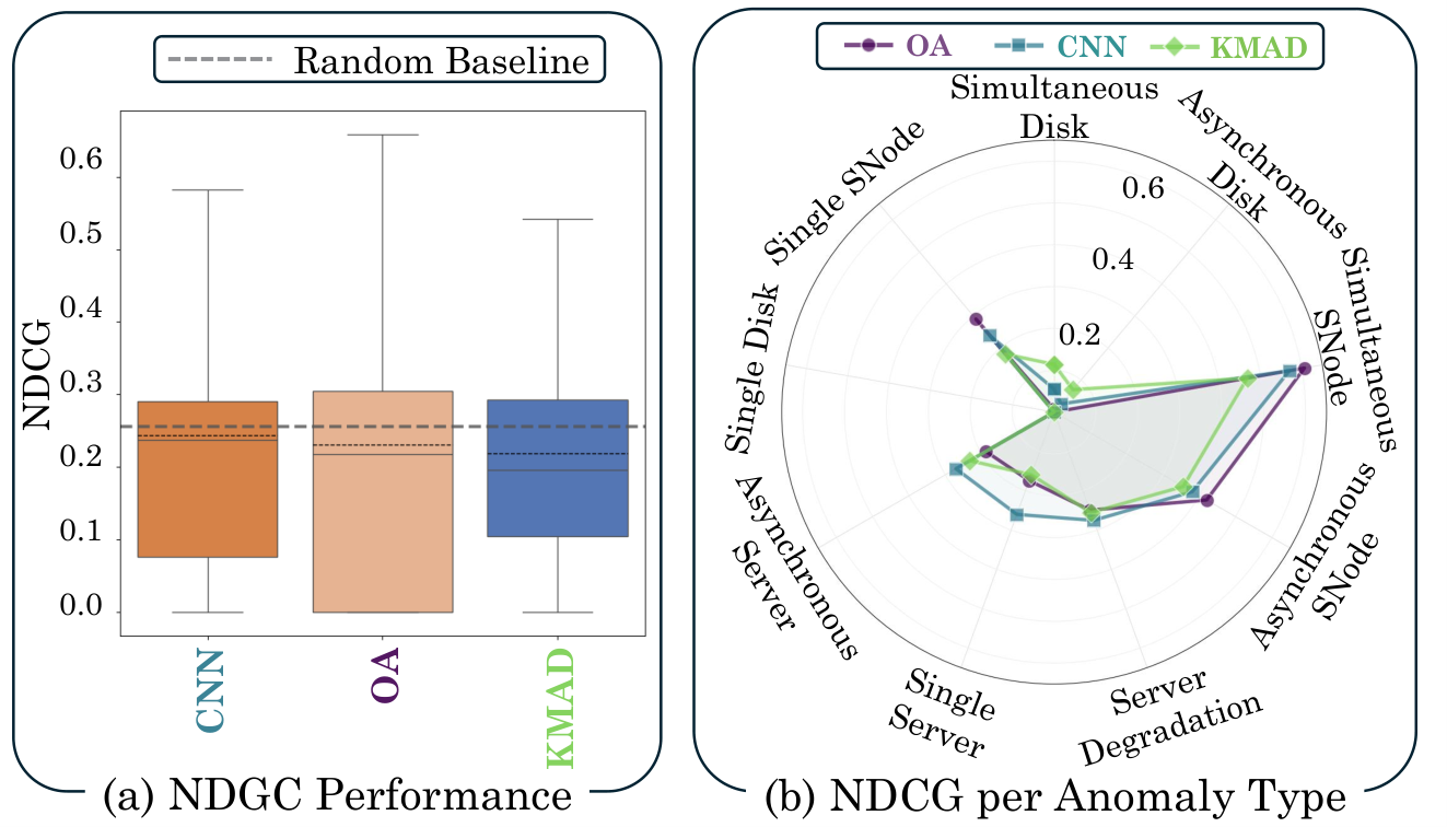
Beyond anomaly detection accuracy, we also evaluate the native capacity of the best performing methods to accurately localize the anomalies across the feature space. We select three representative methods: OA (Semi-Supervised, Reconstruction-based), CNN (Semi-Supervised, Prediction-based) and KMAD (Unsupervised, Clustering-based), and derive their feature-wise scores. Results in Figure 8 (a) reveal a striking observation: despite their strong detection performance, the methods exhibit behavior nearly indistinguishable from a random baseline in term of dimension localization. This highlights that good detection accuracy does not inherently translate into diagnostic utility, and internal scoring mechanisms of these methods are not natively designed for feature attribution. The granular analysis on the anomaly type in Figure 8 (b) confirms this observation. The worst results (Single Disk, Simultaneous Disk and Asynchronous Disk) have a low dimensional contamination rate (respectively 4, 12 and 12 dimensions contaminated on average) while the best localized anomalies, Simultaneous SNode, have on average 140 anomalous dimensions.

4.3 RQ3: Time Series Anomaly Interpretation

Comparison with different representations. Figure 9(a) reports the performance of LLMs across different input representations for the interpretability task. Overall, results are very low, highlighting the difficulty of interpreting high-dimensional real-world time series. For anomaly presence ( ), most of the LLMs always predicted an anomaly regardless of the representation, suggesting that irregular patterns and high-dimensionality lead the models to interpret variability as anomalies. This led to very similar average results across all models (0.48, 0.47, 0.43 for Descriptions, Images, and Catch22, resp.). For anomaly type, performance remains poor, with the best F1-score from Images ( $21\%$ ), followed by Catch22 ( $19\%$ ) and descriptions ( $14\%$ ), and a noticeable bias toward Disk Failures. The anomaly criticality task ( ) is even more challenging, with a maximum of $16\%$ (Images), showing the inability to assess severity without contextual knowledge. Dimension localization ( ) is among the hardest tasks, with near-zero accuracy ( $1\%$ , $2\%$ , $1\%$ for Catch22, Images, and descriptions), reflecting the difficulty of identifying anomalous dimensions in large multivariate data. For time localization ( ), results are slightly better but still low ( $7\%$ , $7\%$ , $2\%$ for Images, Catch22, and Descriptions). Overall, all the results highlighted the complexity of interpreting time series using LLMs without any type of supervision. While the results are generally low, providing Images was the best option for three tasks ( , , ) and the second best option for the others, suggesting that visual representations provide a slightly clearer overview of the series.

Comparison with different LLMs. Figure 9(a) compares the performance of 5 LLMs for each representation across the five tasks. For anomaly presence ( ), almost all models behaved identically ( $\approx 47\%$ across all representations), showing a strong bias towards anomalies. The only exception was Grok (especially with the Catch22 representation) which, in contrast, judged most series as normal. This is consistent with recent evidence that Grok exhibits a distinctive behavioral profile compared to other frontier LLMs [105]. For anomaly type and criticality ( , ) the best LLM is Claude ( $0.23$ and $0.19$ , resp.), while Grok was the best for dimension localization ( ), but with only 4% of accuracy. Finally, Claude was the best model for time localization ( ), with 12%. Overall, all the models showed very similar behaviours (we provide the full results in Appendix E), showing that interpreting anomalies is a significant challenge.

Adding supervison. We evaluate LLM performance under two supervision levels, simulating the interpretability step when detection and explanation outputs are available. Figure 9(b) reports results across all models and representations. For clarity, we omit tasks directly answered by supervision (accuracy $=1.0$ ). With level₁ (i.e., anomaly presence), performance consistently improves for dimension and time localization ( , ), with average gains of $7.2\%$ and $7.9\%$ . Although results remain low, this indicates that additional information can help characterize anomalies. For other tasks, trends are inconsistent, with negligible variation (below $0.2\%$ ). With level₂ (i.e., anomaly presence + affected components), further improvements are observed for time localization ( ) (+ $14.4\%$ ) and anomaly type ( ) (+ $4.7\%$ ), while anomaly criticality shows negligible change. Overall, although combining detection and explanation signals improves performance, zero-shot LLMs remain unable to reliably characterize anomalies, highlighting the need for domain-specific solutions.

Comparison with smaller LLMs. Figure 10(a) compares the performance of Mistral Large, Medium, and Small. With Mistral Medium, we observe a significant drop when using Catch22, likely due to the difficulty of reasoning over many statistical features across high-dimensional data. In contrast, performance with Images remains stable and even improves on time localization ( ) ( $14\%$ vs. $7\%$ ). Results with Image Descriptions are nearly identical to the largest model. With Mistral Small, performance generally drops, highlighting its limited capacity to handle both high-dimensional statistical features and richer multimodal inputs, leading to consistently lower results across tasks.

5 Conclusion and Future directions

We proposed SHAD, a novel end-to-end benchmark composed of real-world, high-dimensional time series, that covers all the steps in TSAD pipelines (detection, explanation, and interpretation). SHAD includes both normal and anomalous series, with anomalies affecting different components and severity levels, and provides per-dimension labels along with rich textual annotations for each dimension and anomaly. Our experimental evaluation concluded that (i) SOTA anomaly detection approaches are accurate but not perfect for all anomalies in SHAD, (ii) Explanability on SHAD cannot be natively solved with existing TSAD methods, and (iii) frozen LLMs are not able to provide correct interpretations of anomalies. Finally, SHAD enables new research directions: in detection, studying robustness when directly affected metrics are removed; in explainability, rigorously assessing variable contributions via per-dimension labels and developing dedicated explainability methods trained on SHAD’s annotations, rather than relying on native detector attribution scores; and in interpretability, investigating how reliable dimension-level explanations can be provided as structured, semantically enriched context to LLMs, enabling the generation of human-understandable anomaly interpretations grounded in both data and semantics.

Acknowledgments and Disclosure of Funding

The authors are grateful to the CLEPS infrastructure from the Inria of Paris for providing resources and support.

References

[1] A. Abdulaal, Z. Liu, and T. Lancewicki (2021) Practical approach to asynchronous multivariate time series anomaly detection and localization. In Proceedings of the 27th ACM SIGKDD conference on knowledge discovery & data mining, pp. 2485–2494. Cited by: Table 2.
[2] C. C. Aggarwal (2015) Outlier analysis. Springer. Cited by: Table 12.
[3] S. Ahmad, A. Lavin, S. Purdy, and Z. Agha (2017) Unsupervised real-time anomaly detection for streaming data. Neurocomputing 262, pp. 134–147. Cited by: §1.
[4] J. Antoni and P. Borghesani (2019) A statistical methodology for the design of condition indicators. Mechanical Systems and Signal Processing 114, pp. 290–327. External Links: Document Cited by: §1, §2.
[5] J. Audibert, P. Michiardi, F. Guyard, S. Marti, and M. A. Zuluaga (2020) USAD: unsupervised anomaly detection on multivariate time series. In Proceedings of the 26th ACM SIGKDD International Conference on Knowledge Discovery & Data Mining, KDD ’20, New York, NY, USA. External Links: ISBN 9781450379984 Cited by: Table 12.
[6] J. Audibert, P. Michiardi, F. Guyard, S. Marti, and M. A. Zuluaga (2022) Do deep neural networks contribute to multivariate time series anomaly detection?. Pattern Recognit. 132, pp. 108945. External Links: Link, Document Cited by: §4.1.
[7] M. Bachlin, M. Plotnik, D. Roggen, I. Maidan, J. M. Hausdorff, N. Giladi, and G. Troster (2009) Wearable assistant for parkinson’s disease patients with the freezing of gait symptom. IEEE Transactions on Information Technology in Biomedicine 14 (2), pp. 436–446. Cited by: Table 2.
[8] J. Bai and S. Ng (2008) Forecasting economic time series using targeted predictors. Journal of Econometrics 146 (2). Cited by: §1.
[9] P. Bailis, E. Gan, S. Madden, D. Narayanan, K. Rong, and S. Suri (2017) Macrobase: prioritizing attention in fast data. In Proceedings of the 2017 ACM International Conference on Management of Data, pp. 541–556. Cited by: §A.3, §2.
[10] L. Bertossi, J. Li, M. Schleich, D. Suciu, and Z. Vagena (2020) Causality-based explanation of classification outcomes. In Proceedings of the Fourth International Workshop on Data Management for End-to-End Machine Learning, pp. 1–10. Cited by: §A.3, §2.
[11] P. Boniol, A. K. Krishna, M. Bruel, Q. Liu, M. Huang, T. Palpanas, R. S. Tsay, A. Elmore, M. J. Franklin, and J. Paparrizos (2025) VUS: effective and efficient accuracy measures for time-series anomaly detection. arXiv preprint arXiv:2502.13318. Cited by: §4.
[12] P. Boniol, Q. Liu, M. Huang, T. Palpanas, and J. Paparrizos (2024) Dive into time-series anomaly detection: a decade review. arXiv preprint arXiv:2412.20512. Cited by: §1.
[13] P. Boniol and T. Palpanas (2020) Series2Graph: graph-based subsequence anomaly detection for time series. Proc. VLDB Endow. 13 (12), pp. 1921–1934. Cited by: §2.
[14] P. Boniol, J. Paparrizos, T. Palpanas, and M. J. Franklin (2021) SAND: streaming subsequence anomaly detection.. Proc. VLDB Endow. 14 (10), pp. 1717–1729. Cited by: Table 2.
[15] A. Boubekki, K. Patlatzoglou, J. Barker, H. Aggour, F. S. Ng, and A. H. Ribeiro (2026) Explaining deep learning for ecg using time-localized clusters. IEEE Transactions on Biomedical Engineering. Cited by: §2.
[16] M. M. Breunig, H. Kriegel, R. T. Ng, and J. Sander (2000) LOF: identifying density-based local outliers. SIGMOD Rec. 29 (2), pp. 93–104. External Links: ISSN 0163-5808, Document Cited by: Table 12.
[17] L. M. Candanedo and V. Feldheim (2016) Accurate occupancy detection of an office room from light, temperature, humidity and co2 measurements using statistical learning models. Energy and buildings 112, pp. 28–39. Cited by: Table 2.
[18] H. Chen, W. Guo, W. Bao, M. Cui, X. Wang, and Q. Zhao (2025) A novel interpretable decision rule extracting method for deep reinforcement learning-based energy management in building complexes. Energy and Buildings 334, pp. 115514. Cited by: §A.3, §2.
[19] B. Dadashova, X. Li, S. Turner, and P. Koeneman (2021) Multivariate time series analysis of traffic congestion measures in urban areas as they relate to socioeconomic indicators. Socio-Economic Planning Sciences 75. Cited by: §1.
[20] H. Dong, B. Liu, D. Ye, and G. Liu (2024) Interpretability as approximation: understanding black-box models by decision boundary. Electronics 13 (22), pp. 4339. Cited by: §A.3, §2.
[21] P. Filonov, A. Lavrentyev, and A. Vorontsov (2016) Multivariate industrial time series with cyber-attack simulation: fault detection using an lstm-based predictive data model. arXiv preprint arXiv:1612.06676. Cited by: Table 2.
[22] P. Fleith (2023) Controlled anomalies time series (cats) dataset. Solenix Engineering GmbH. Cited by: Table 2.
[23] N. Frosst and G. Hinton (2017) Distilling a neural network into a soft decision tree. arXiv preprint arXiv:1711.09784. Cited by: §A.3, §2.
[24] Y. Gao, J. Lin, and C. Brif (2020) Ensemble grammar induction for detecting anomalies in time series. In Proceedings of the 23rd International Conference on Extending Database Technology, EDBT 2020, Copenhagen, Denmark, March 30 - April 02,2020, pp. 85–96. External Links: Document Cited by: §1, §2.
[25] S. Ghassempour, F. Girosi, and A. Maeder (2014) Clustering multivariate time series using hidden markov models. IJERPH 11 (3). Cited by: §1.
[26] J. Goh, S. Adepu, K. N. Junejo, and A. Mathur (2016) A dataset to support research in the design of secure water treatment systems. In International conference on critical information infrastructures security, pp. 88–99. Cited by: Table 2.
[27] A. L. Goldberger, L. A. Amaral, L. Glass, J. M. Hausdorff, P. C. Ivanov, R. G. Mark, J. E. Mietus, G. B. Moody, C. Peng, and H. E. Stanley (2000) PhysioBank, physiotoolkit, and physionet: components of a new research resource for complex physiologic signals. circulation 101 (23), pp. e215–e220. Cited by: Table 2, Table 2.
[28] M. Goldstein and A. R. Dengel (2012) Histogram-based outlier score (hbos): a fast unsupervised anomaly detection algorithm. Cited by: Table 12.
[29] S. D. Greenwald, R. S. Patil, and R. G. Mark (1990) Improved detection and classification of arrhythmias in noise-corrupted electrocardiograms using contextual information. IEEE. Cited by: Table 2.
[30] N. Gruver, M. Finzi, S. Qiu, and A. G. Wilson (2023) Large language models are zero-shot time series forecasters. Advances in neural information processing systems 36, pp. 19622–19635. Cited by: §A.3, §1, §2.
[31] Z. He, X. Xu, and S. Deng (2003) Discovering cluster-based local outliers. Pattern Recognition Letters 24 (9-10), pp. 1641–1650. External Links: ISSN 0167-8655, Document, Link Cited by: Table 12.
[32] A. Heuillet, F. Couthouis, and N. Díaz-Rodríguez (2021) Explainability in deep reinforcement learning. Knowledge-Based Systems 214, pp. 106685. Cited by: §2.
[33] K. Hundman, V. Constantinou, C. Laporte, I. Colwell, and T. Soderstrom (2018) Detecting spacecraft anomalies using lstms and nonparametric dynamic thresholding. In Proceedings of the 24th ACM SIGKDD international conference on knowledge discovery & data mining, pp. 387–395. Cited by: Table 2, Table 2.
[34] A. Ihler, J. Hutchins, and P. Smyth (2006) Adaptive event detection with time-varying poisson processes. In Proceedings of the 12th ACM SIGKDD International Conference on Knowledge Discovery and Data Mining, KDD ’06, New York, NY, USA, pp. 207–216. External Links: ISBN 1595933395, Link, Document Cited by: Table 2.
[35] IOPS. Note: http://iops.ai/dataset_detail/?id=10 Cited by: Table 2.
[36] V. Jacob, F. Song, A. Stiegler, B. Rad, Y. Diao, and N. Tatbul (2020) Exathlon: a benchmark for explainable anomaly detection over time series. arXiv preprint arXiv:2010.05073. Cited by: §A.1, §A.3, §1, §2, §2, Table 1.
[37] M. Jin, S. Wang, L. Ma, Z. Chu, J. Y. Zhang, X. Shi, P. Chen, Y. Liang, Y. Li, S. Pan, et al. (2023) Time-llm: time series forecasting by reprogramming large language models. arXiv preprint arXiv:2310.01728. Cited by: §A.3, §2.
[38] M. Jin, Y. Zhang, W. Chen, K. Zhang, Y. Liang, B. Yang, J. Wang, S. Pan, and Q. Wen (2024) Position: what can large language models tell us about time series analysis. In Forty-first international conference on machine learning, Cited by: §A.3, §2.
[39] E. Keogh, J. Lin, S. Lee, and H. V. Herle (2007) Finding the most unusual time series subsequence: algorithms and applications. Knowledge and Information Systems 11 (1), pp. 1–27. Cited by: Table 2.
[40] E. Keogh, S. Lonardi, C. A. Ratanamahatana, L. Wei, S. Lee, and J. Handley (2007) Compression-based data mining of sequential data. Data Mining and Knowledge Discovery 14 (1), pp. 99–129. Cited by: §2.
[41] E. M. Knorr and R. T. Ng (1998) Algorithms for mining distance-based outliers in large datasets. In Proceedings of the 24rd International Conference on Very Large Data Bases, VLDB ’98, San Francisco, CA, USA, pp. 392–403. External Links: ISBN 1558605665 Cited by: Table 12.
[42] M. Kopp, T. Pevnỳ, and M. Holeňa (2020) Anomaly explanation with random forests. Expert Systems with Applications 149, pp. 113187. Cited by: §A.3, §2.
[43] L. J. Kurisinkel, P. Mishra, and Y. Zhang (2024) Text2timeseries: enhancing financial forecasting through time series prediction updates with event-driven insights from large language models. arXiv preprint arXiv:2407.03689. Cited by: §A.3, §2.
[44] K. Lai, D. Zha, J. Xu, Y. Zhao, G. Wang, and X. Hu (2021) Revisiting time series outlier detection: definitions and benchmarks. In Thirty-fifth conference on neural information processing systems datasets and benchmarks track (round 1), Cited by: §A.1, §2, Table 1.
[45] S. Lai, Z. Xu, W. Zhang, H. Liu, and H. Xiong (2025) LLMLight: large language models as traffic signal control agents. In Proceedings of the 31st ACM SIGKDD Conference on Knowledge Discovery and Data Mining V. 1, pp. 2335–2346. Cited by: §A.3, §2.
[46] H. Lakkaraju, S. H. Bach, and J. Leskovec (2016) Interpretable decision sets: a joint framework for description and prediction. In Proceedings of the 22nd ACM SIGKDD international conference on knowledge discovery and data mining, pp. 1675–1684. Cited by: §A.3, §2.
[47] N. Laptev, S. Amizadeh, and Y. Billawala (2015) S5-a labeled anomaly detection dataset, version 1.0 (16m). URL https://webscope. sandbox. yahoo. com/catalog. php. Cited by: Table 2.
[48] A. Lavin and S. Ahmad (2015) Evaluating real-time anomaly detection algorithms–the numenta anomaly benchmark. In 2015 IEEE 14th international conference on machine learning and applications (ICMLA), pp. 38–44. Cited by: §A.1, §2, Table 1.
[49] J. Lee, B. Park, and D. Chae (2023) Duogat: dual time-oriented graph attention networks for accurate, efficient and explainable anomaly detection on time-series. In Proceedings of the 32nd ACM international conference on information and knowledge management, pp. 1188–1197. Cited by: §2.
[50] M. Linardi, Y. Zhu, T. Palpanas, and E. Keogh (2020) Matrix profile goes mad: variable-length motif and discord discovery in data series. arXiv preprint arXiv:2008.13447. Cited by: §2.
[51] F. T. Liu, K. M. Ting, and Z. Zhou (2008) Isolation forest. In 2008 eighth ieee international conference on data mining, pp. 413–422. Cited by: Table 12, §2.
[52] Q. Liu and J. Paparrizos (2024) The elephant in the room: towards a reliable time-series anomaly detection benchmark. Advances in Neural Information Processing Systems 37, pp. 108231–108261. Cited by: §A.1, §2, §2, Table 1, §3, §4.
[53] Y. Liu, X. Chen, F. Wang, and J. Yin (2009) Efficient detection of discords for time series stream. In Asia-Pacific Web Conference, pp. 629–634. Cited by: §2.
[54] C. H. Lubba, S. S. Sethi, P. Knaute, S. R. Schultz, B. D. Fulcher, and N. S. Jones (2019) Catch22: canonical time-series characteristics. arXiv preprint arXiv:1901.10200. Cited by: §4.
[55] S. M. Lundberg and S. Lee (2017) A unified approach to interpreting model predictions. Advances in neural information processing systems 30. Cited by: §A.3, §2.
[56] P. Malhotra, L. Vig, G. M. Shroff, and P. Agarwal (2015) Long short term memory networks for anomaly detection in time series. In The European Symposium on Artificial Neural Networks, Cited by: Table 12.
[57] Metro. Note: https://www.kaggle.com/datasets/pooriamst/metro-interstate-traffic-volume Cited by: Table 2.
[58] C. Molnar (2020) Interpretable machine learning. Lulu. com. Cited by: §A.3, §2.
[59] S. Moritz, F. Rehbach, S. Chandrasekaran, M. Rebolledo, and T. Bartz-Beielstein (2018) Gecco industrial challenge 2018 dataset: a water quality dataset for the ‘internet of things: online anomaly detection for drinking water quality’competition at the genetic and evolutionary computation conference 2018, kyoto, japan. Kyoto, Japan. Cited by: Table 2.
[60] M. Munir, S. A. Siddiqui, A. Dengel, and S. Ahmed (2018) DeepAnT: a deep learning approach for unsupervised anomaly detection in time series. IEEE access 7, pp. 1991–2005. Cited by: Table 12.
[61] A. Nayebi, S. Tipirneni, C. K. Reddy, B. Foreman, and V. Subbian (2023) WindowSHAP: an efficient framework for explaining time-series classifiers based on shapley values. Journal of biomedical informatics 144, pp. 104438. Cited by: §A.3, §2.
[62] J. Oh, G. Lee, S. Bae, J. Kwon, and E. Choi (2023) Ecg-qa: a comprehensive question answering dataset combined with electrocardiogram. Advances in Neural Information Processing Systems 36, pp. 66277–66288. Cited by: §A.3, §2.
[63] R. Paffenroth, K. Kay, and L. Servi (2018) Robust pca for anomaly detection in cyber networks. arXiv preprint arXiv:1801.01571. Cited by: Table 12.
[64] T. Palpanas (2015) Data series management: the road to big sequence analytics. ACM SIGMOD Record 44 (2), pp. 47–52. Cited by: §1.
[65] J. Paparrizos, P. Boniol, T. Palpanas, R. S. Tsay, A. J. Elmore, and M. J. Franklin (2022) Volume under the surface: a new accuracy evaluation measure for time-series anomaly detection.. Proc. VLDB Endow. 15 (11), pp. 2774–2787. Cited by: §4.
[66] J. Paparrizos, Y. Kang, P. Boniol, R. S. Tsay, T. Palpanas, and M. J. Franklin (2022) TSB-uad: an end-to-end benchmark suite for univariate time-series anomaly detection.. Proc. VLDB Endow. 15 (8), pp. 1697–1711. Cited by: §A.1, §1, §2, §2, Table 1.
[67] X. Qiu, Z. Li, W. Qiu, S. Hu, L. Zhou, X. Wu, Z. Li, C. Guo, A. Zhou, Z. Sheng, et al. (2025) Tab: unified benchmarking of time series anomaly detection methods. arXiv preprint arXiv:2506.18046. Cited by: §A.1, §2, Table 1.
[68] K. Rasul, A. Ashok, A. R. Williams, H. Ghonia, R. Bhagwatkar, A. Khorasani, M. J. D. Bayazi, G. Adamopoulos, R. Riachi, N. Hassen, et al. (2023) Lag-llama: towards foundation models for probabilistic time series forecasting. arXiv preprint arXiv:2310.08278. Cited by: §A.3, §2.
[69] M. T. Ribeiro, S. Singh, and C. Guestrin (2016) " Why should i trust you?" explaining the predictions of any classifier. In Proceedings of the 22nd ACM SIGKDD international conference on knowledge discovery and data mining, pp. 1135–1144. Cited by: §A.3, §2.
[70] M. T. Ribeiro, S. Singh, and C. Guestrin (2018) Anchors: high-precision model-agnostic explanations. In Proceedings of the AAAI conference on artificial intelligence, Vol. 32. Cited by: §A.3, §2.
[71] D. Roggen, A. Calatroni, M. Rossi, T. Holleczek, K. Förster, G. Tröster, P. Lukowicz, D. Bannach, G. Pirkl, A. Ferscha, et al. (2010) Collecting complex activity datasets in highly rich networked sensor environments. In 2010 Seventh international conference on networked sensing systems (INSS), pp. 233–240. Cited by: Table 2.
[72] P. J. Rousseeuw (1984) Least median of squares regression. Journal of the American Statistical Association 79 (388), pp. 871–880. External Links: Document Cited by: Table 12.
[73] M. Sakurada and T. Yairi (2014) Anomaly detection using autoencoders with nonlinear dimensionality reduction. In Proceedings of the MLSDA 2014 2nd workshop on machine learning for sensory data analysis, pp. 4–11. Cited by: Table 12.
[74] S. Schmidl, P. Wenig, and T. Papenbrock (2022) Anomaly detection in time series: a comprehensive evaluation. Cited by: §A.1, §2, Table 1.
[75] B. Schölkopf, R. C. Williamson, A. Smola, J. Shawe-Taylor, and J. Platt (1999) Support vector method for novelty detection. Advances in neural information processing systems 12. Cited by: Table 12.
[76] I. Sharafaldin, A. H. Lashkari, A. A. Ghorbani, et al. (2018) Toward generating a new intrusion detection dataset and intrusion traffic characterization.. ICISSp 1 (2018), pp. 108–116. Cited by: Table 2.
[77] H. Si, J. Li, C. Pei, H. Cui, J. Yang, Y. Sun, S. Zhang, J. Li, H. Zhang, J. Han, et al. (2024) Timeseriesbench: an industrial-grade benchmark for time series anomaly detection models. In 2024 IEEE 35th International Symposium on Software Reliability Engineering (ISSRE), pp. 61–72. Cited by: Table 2.
[78] I. Stoica, R. Morris, D. Liben-Nowell, D. R. Karger, M. F. Kaashoek, F. Dabek, and H. Balakrishnan (2003) Chord: a scalable peer-to-peer lookup protocol for internet applications. IEEE/ACM Transactions on networking 11 (1), pp. 17–32. Cited by: §D.1, §3.
[79] Y. Su, Y. Zhao, C. Niu, R. Liu, W. Sun, and D. Pei (2019) Robust anomaly detection for multivariate time series through stochastic recurrent neural network. In Proceedings of the 25th ACM SIGKDD International Conference on Knowledge Discovery and Data Mining, KDD ’19, pp. 2828–2837. External Links: ISBN 9781450362016, Document Cited by: §A.3, Table 12, §2, §2.
[80] Y. Su, Y. Zhao, C. Niu, R. Liu, W. Sun, and D. Pei (2019) Robust anomaly detection for multivariate time series through stochastic recurrent neural network. In Proceedings of the 25th ACM SIGKDD international conference on knowledge discovery & data mining, pp. 2828–2837. Cited by: Table 2, Table 2.
[81] M. Sundararajan, A. Taly, and Q. Yan (2017) Axiomatic attribution for deep networks. In International conference on machine learning, pp. 3319–3328. Cited by: §A.3, §2.
[82] E. Sylligardos, P. Boniol, J. Paparrizos, P. Trahanias, and T. Palpanas (2023) Choose wisely: an extensive evaluation of model selection for anomaly detection in time series. Proceedings of the VLDB Endowment 16 (11), pp. 3418–3432. Cited by: §A.1, §2.
[83] Tao. Note: http://pmel.noaa.gov/ Cited by: Table 2.
[84] M. Thill, W. Konen, and T. Bäck (2020) MarkusThill/mgab: the mackey–glass anomaly benchmark. version v1. 0.0. zenodo. Cited by: Table 2.
[85] L. Tran, L. Fan, and C. Shahabi (2016) Distance-based outlier detection in data streams. Proceedings of the VLDB Endowment 9 (12), pp. 1089–1100. Cited by: Table 2.
[86] A. von Birgelen and O. Niggemann (2018) Anomaly detection and localization for cyber-physical production systems with self-organizing maps. In IMPROVE-Innovative Modelling Approaches for Production Systems to Raise Validatable Efficiency: Intelligent Methods for the Factory of the Future, pp. 55–71. Cited by: Table 2.
[87] D. Wagner, T. Michels, F. C. Schulz, A. Nair, M. Rudolph, and M. Kloft (2023) Timesead: benchmarking deep multivariate time-series anomaly detection. Transactions on Machine Learning Research. Cited by: §A.1, §2, Table 1.
[88] X. Wang, M. Feng, J. Qiu, J. Gu, and J. Zhao (2024) From news to forecast: integrating event analysis in llm-based time series forecasting with reflection. Advances in Neural Information Processing Systems 37, pp. 58118–58153. Cited by: §A.3, §2.
[89] Y. Wang, L. Wang, Y. Li, D. He, and T. Liu (2013) A theoretical analysis of ndcg type ranking measures. In Proceedings of the 26th Annual Conference on Learning Theory, S. Shalev-Shwartz and I. Steinwart (Eds.), Proceedings of Machine Learning Research, Vol. 30, Princeton, NJ, USA, pp. 25–54. External Links: Link Cited by: §4.
[90] Z. Wang, Z. Liu, Y. Zhang, A. Zhong, J. Wang, F. Yin, L. Fan, L. Wu, and Q. Wen (2024) Rcagent: cloud root cause analysis by autonomous agents with tool-augmented large language models. In Proceedings of the 33rd ACM international conference on information and knowledge management, pp. 4966–4974. Cited by: §A.3, §2.
[91] P. Wenig and T. Papenbrock (2024) Series2graph++: distributed detection of correlation anomalies in multivariate time series. In International Conference on Big Data Analytics and Knowledge Discovery, pp. 225–230. Cited by: §1.
[92] E. Winter (2002) The shapley value. Handbook of game theory with economic applications 3, pp. 2025–2054. Cited by: §A.3, §2.
[93] H. Wu, T. Hu, Y. Liu, H. Zhou, J. Wang, and M. Long (2022) Timesnet: temporal 2d-variation modeling for general time series analysis. arXiv preprint arXiv:2210.02186. Cited by: Table 12.
[94] R. Wu and E. J. Keogh (2021) Current time series anomaly detection benchmarks are flawed and are creating the illusion of progress. IEEE transactions on knowledge and data engineering 35 (3), pp. 2421–2429. Cited by: §A.1, Table 2.
[95] W. Wu, L. He, W. Lin, Y. Su, Y. Cui, C. Maple, and S. Jarvis (2022) Developing an unsupervised real-time anomaly detection scheme for time series with multi-seasonality. IEEE Transactions on Knowledge and Data Engineering 34 (9), pp. 4147–4160. External Links: ISSN 2326-3865, Link, Document Cited by: §A.3, §2, §2.
[96] Z. Xie, Z. Li, X. He, L. Xu, X. Wen, T. Zhang, J. Chen, R. Shi, and D. Pei (2024) Chatts: aligning time series with llms via synthetic data for enhanced understanding and reasoning. arXiv preprint arXiv:2412.03104. Cited by: §A.3, §1, §2, footnote 2.
[97] T. Xing, L. Garcia, F. Cerutti, L. Kaplan, A. Preece, and M. Srivastava (2021) Deepsqa: understanding sensor data via question answering. In Proceedings of the International Conference on Internet-of-Things Design and Implementation, pp. 106–118. Cited by: §A.3, §2.
[98] J. Xu, H. Wu, J. Wang, and M. Long (2021) Anomaly transformer: time series anomaly detection with association discrepancy. arXiv preprint arXiv:2110.02642. Cited by: Table 12.
[99] Z. Xu, A. Zeng, and Q. Xu (2023) FITS: modeling time series with $10k$ parameters. arXiv preprint arXiv:2307.03756. Cited by: Table 12.
[100] T. Yairi, Y. Kato, and K. Hori (2001) Fault detection by mining association rules from house-keeping data. In proceedings of the 6th International Symposium on Artificial Intelligence, Robotics and Automation in Space, Vol. 18, pp. 21. Cited by: Table 12.
[101] Y. Yao, A. Sharma, L. Golubchik, and R. Govindan (2010) Online anomaly detection for sensor systems: a simple and efficient approach. Performance Evaluation 67 (11), pp. 1059–1075. Cited by: Table 2.
[102] C. M. Yeh, Y. Zhu, L. Ulanova, N. Begum, Y. Ding, H. A. Dau, D. F. Silva, A. Mueen, and E. Keogh (2016) Matrix profile i: all pairs similarity joins for time series: a unifying view that includes motifs, discords and shapelets. In 2016 IEEE 16th international conference on data mining (ICDM), pp. 1317–1322. Cited by: §2.
[103] A. Zhang, S. Deng, D. Cui, Y. Yuan, and G. Wang (2023) An experimental evaluation of anomaly detection in time series. Proceedings of the VLDB Endowment 17 (3), pp. 483–496. Cited by: §A.1, §2, Table 1.
[104] H. Zhang, Y. Diao, and A. Meliou (2017) Exstream: explaining anomalies in event stream monitoring. In Proceedings of the 20th international conference on extending database technology (EDBT), Cited by: §A.3.
[105] J. Zhang, H. Sleight, A. Peng, J. Schulman, and E. Durmus (2025) Stress-testing model specs reveals character differences among language models. arXiv preprint arXiv:2510.07686. Cited by: §4.3.
[106] S. Zhang, Z. Zhong, D. Li, Q. Fan, Y. Sun, M. Zhu, Y. Zhang, D. Pei, J. Sun, Y. Liu, et al. (2022) Efficient kpi anomaly detection through transfer learning for large-scale web services. IEEE Journal on Selected Areas in Communications 40 (8), pp. 2440–2455. Cited by: Table 2.
[107] T. Zhou, P. Niu, L. Sun, R. Jin, et al. (2023) One fits all: power general time series analysis by pretrained lm. Advances in neural information processing systems 36, pp. 43322–43355. Cited by: §A.3, §1, §2.
[108] X. Zhou, G. Li, Z. Sun, Z. Liu, W. Chen, J. Wu, J. Liu, R. Feng, and G. Zeng (2023) D-bot: database diagnosis system using large language models. arXiv preprint arXiv:2312.01454. Cited by: §A.3, §2.
[109] J. Zhuang, L. Yan, Z. Zhang, R. Wang, J. Zhang, and Y. Gu (2024) See it, think it, sorted: large multimodal models are few-shot time series anomaly analyzers. arXiv preprint arXiv:2411.02465. Cited by: §A.3, §1, §2.

Appendix A Related Work

A.1 Existing benchmarks

Existing Benchmarks: How do we evaluate time series anomaly detection?

Research in TSAD has led to the introduction of numerous datasets (see Table 2), which have been considered in multiple surveys [66, 74, 82, 52], consistently highlighting the absence of a one-size-fits-all anomaly detector. Consequently, efforts have aimed to establish benchmarks, whose main characteristics are detailed in Table 1, incorporating multiple datasets from various domains for comprehensive evaluation. NAB [48] provides 58 labeled real-world and artificial time series, and primarily focuses on real-time anomaly detection for streaming data. It comprises diverse domains such as AWS server metrics, online advertisement clicking rates, real-time traffic data, and a collection of Twitter mentions of large publicly-traded companies. TODS [44] refines synthetic criterion and includes five anomaly scenarios categorized as point-global, pattern-contextual, pattern-shapelet, pattern-seasonal, and pattern-trend. TimeEval [74] comprises a collection of datasets (both real/synthetic and univariate/multivariate) with point and sequence anomalies. In addition, this benchmark has been filtered such that there is no time series that has a normal/abnormal ratio above $0.1$ , and that at least one method performs more than 0.8 AUC-ROC for each time series. TimeSeAD [87] analyzed widely used multivariate datasets and introduced a recall-consistent evaluation metric that accounts for temporal correlations, benchmarking 28 deep-learning based methods, while Experimental-TSAD [103] compared 17 state-of-the-art anomaly detection methods using both point-based and range-based metrics across various data sizes, anomaly rates, feature dimensions, and temporal patterns. TSB-UAD [66] is a comprehensive benchmark designed for evaluating univariate TSAD, including real-world and synthetic datasets. Exathlon [36] is proposed for explainable anomaly detection over high-dimensional time series data. It is constructed based on real data traces from an Apache Spark cluster, and was designed to address the pitfalls of previous benchmarks [94]. It features a single anomalies per series, which in most cases is artificially. Aiming at addressing the challenge of designing truly representative benchmarks, TSB-AD [52] introduced the first large-scale, heterogeneous, and meticulously curated dataset, also incorporating latest advances in foundation model-based methods, highlighting their potential for TSAD. Finally, TAB [67] is a recent and comprehensive benchmark that provides an extensive algorithmic comparison, including 19 statistical methods, 18 neural network–based approaches, and 7 foundation model–based methods.

A.2 TSAD Datasets

Table 2 lists the datasets for time series anomaly detection currently available in the literature. For each one, we report the key characteristics, including the number of available time series and their average lenght and dimensionality, the type of anomalies, and the domain from which they belong.

A.3 Interpretability and Explainability

Interpretable and Explainable Anomaly Detection.

Explainable machine learning techniques can be broadly categorized into intrinsically explainable models and model-agnostic approaches [36]. The former category focuses on building a human-readable representation (e.g. decision trees) from data [58], while the latter separate explanations from the ML model [69]. From the perspective of anomaly detection approaches, all forecasting/reconstruction methods [95, 79] are inherently explainable. Among model-agnostic approaches, several methods are based on perturbing the inputs and observing the response of the classifier [46]. LIME [69] explains individual predictions by learning a local surrogate model that approximates the original model in the neighborhood of a given instance, using a weighted linear regression formulation. This framework was extended by Anchors [70], which replaces the linear model with logical rules. Other approaches assign a numerical score to each feature [10, 81], indicating its importance in the classification of each instance. Among these, SHAP [55] provides a theoretically grounded measure of feature importance based on Shapley values [92], and has been recently extended to support time series data [61]. Other approaches focus on providing global explanations, approximating deep-learning classifiers with explainable models [23, 20] or by learning decision rules [42, 46, 18].

In the context of anomaly detection, the literature on interpretable approaches is rather limited. Among existing methods, MacroBase [9] supports the user by prioritizing their attention on specific portions of high-volume data streams and by providing interpretable insights based on the relative recurrence of key attributes. On the other hand, EXstream [104] finds interpretations to distinguish the normal and anomalous periods given as input by the user. Recent advances in large language models (LLMs) represent a promising research direction in this area, enabling the generation of context-rich insights by leveraging model outputs and/or auxiliary information [38]. While many approaches focused on using LLMs for the anomaly detection task itself [37, 88, 68], other have started to explore their usefulness in providing human-understandable data analysis [97, 62]. In particular, recent years have witnessed the introduction of several Time Series Question Answering (TSQA) systems in domains such as healthcare and sensor analytics [97, 62], where natural language interfaces are used to query and interpret raw temporal signals. LLMs have also been explored for integrating time series with external textual context, enabling more informed predictions and decision-making [43, 45]. Agent-based and tool-augmented frameworks further enhance autonomous reasoning and support root cause analysis [90, 108]. While several LLM-based approaches have been proposed [30, 107], only few of them supports multimodal data [109, 96]. Among these, ChatTS [96] is a recent multimodal LLM (MLLM) that can perform both reasoning and understanding on time series. It directly takes multivariate time series as input and enables natural language interaction for interpreting patterns, relationships, and anomalies within the data.

Table 2: Summary characteristics of 30 datasets

Name	Category	Dimension	Avg Dim	# of time series	Avg Length	Domain
UCR [94]	P&S	I	1	250	67818.7	Multiple
Yahoo [47]	P&S	I	1	367	1560.2	Web Service
IOPS [35]	S	I	1	58	72792.3	IT/Web Services
MGAB [84]	S	I	1	10	97777.8	Synthetic
WSD [106]	S	I	1	210	17444.5	IT/Web Services
SED [14]	S	I	1	6	23332.3	Sensor
NEK [77]	P&S	I	1	48	1073.0	IT/Web Services
Stock [85]	P&S	I	1	90	15000.0	Financial
Power [39]	S	I	1	1	35040.0	Facility
SensorScope [101]	S	I	1	23	27038.4	Environmental
Dodgers [34]	S	I	1	1	50400.0	Traffic
Daphnet [7]	S	M	9	17	38774.0	Human Activity
CATSv2 [22]	S	M	17	10	240000.0	Sensor
SWaT [26]	S	M	59	4	207457.5	Sensor
LTDB [27]	S	M	2	7	100000.0	Medical
TAO [83]	P&S	M	3	45	10000.0	Aerospace
MITDB [27]	S	M	2	48	336153.8	Medical
MSL [33]	S	M	55	27	3119.4	Aerospace
SMAP [33]	S	M	25	54	7855.9	Aerospace
SMD [80]	S	M	38	28	25466.4	IT/Web Services
SVDB [29]	S	M	2	78	207122.6	Medical
OPP [71]	S	M	248	24	17426.75	Human Activity
GHL [21]	S	M	19	48	199001.0	Environmental
Genesis [86]	S	M	18	1	16220.0	Sensor
PSM [1]	P&S	M	25	1	217624.0	Facility
CreditCard [76]	P&S	M	29	1	284807.0	Financial
GECCO [59]	S	M	9	1	138521.0	Sensor
SMD [80]	S	M	38	28	25300.7	Facility
Occupancy [17]	S	M	5	2	6208.5	Environmental
Metro [57]	S	M	5	1	48204.0	Traffic

•

I: Univariate; M: Multivariate // P: Point; S: Subsequence
•

The statistics are based on the datasets downloaded during the writing of this article.

Appendix B Metric Catalog

Tables 3–6 provide the complete catalog of all 171 dimensions in the dataset, grouped by hierarchy level. Server-level metrics (Table 5) are replicated across all three storage servers with the naming convention {server}-{metric} (e.g., store1-cpu_usage_ratio), yielding $19\times 3=57$ columns. Device-level metrics (Table 6) follow {server}-{device}-{metric} (e.g., store1-g1disk01-disk_read_bytes), with 7 devices per server and 4 metrics per device, yielding $4\times 7\times 3=84$ columns.

Platform-level metrics include telemetry from the supervisor server, which also hosts the experiment framework. Its contribution is negligible and consistent across all experiments.

Table 3: Platform-level metrics (17 dimensions, cluster-wide aggregates).

Metric	Unit	Description
cpu_usage_ratio	ratio [0,1]	Fraction of CPU time not idle, averaged across all servers.
cpu_load_ratio	ratio [ $\geq$ 0]	CPU load average normalized by CPU count across all servers. Can exceed 1.0 when the run queue exceeds CPU count.
memory_usage_ratio	ratio [0,1]	Fraction of total used memory, averaged across all servers.
network_in_bytes	bytes/s	Total incoming network throughput across all interfaces on all servers.
network_out_bytes	bytes/s	Total outgoing network throughput across all interfaces on all servers.
objects_count	count	Number of objects stored on the RING, including replicas.
objects_unique_count	count	Number of unique logical objects, deduplicated regardless of replica count.
objects_missing_count	count	Number of objects with missing or out-of-service chunks.
capacity_disk_unique_tb	TB	Total stored data of unique objects before replication (logical data size).
capacity_disk_stored_tb	TB	Total stored data including all replicas.
capacity_disk_used_tb	TB	Actual disk space consumed, including storage overhead beyond object data.
capacity_disk_available_tb	TB	Free disk space on the RING.
capacity_disk_total_tb	TB	Total physical disk capacity. Static unless disks are removed.
disk_read_bytes	bytes/s	Total disk read throughput summed across all disks.
disk_write_bytes	bytes/s	Total disk write throughput summed across all disks.
disk_io_time_seconds	s/s [0,1]	Fraction of time spent on I/O, averaged across all disks.
disk_errors_count	count	Number of disk errors across all disks. Always zero in this dataset.

Table 4: S3-level metrics (13 dimensions, aggregated across storage servers).

Metric	Unit	Description
s3_errors_5xx	errors/s	Rate of HTTP 5xx server errors across all S3 services.
s3_request_get_operations	ops/s	GET request rate.
s3_request_post_operations	ops/s	POST request rate. Near-constant (no multipart uploads in the nominal workload).
s3_request_put_operations	ops/s	PUT request rate.
s3_request_delete_operations	ops/s	DELETE request rate.
s3_request_head_operations	ops/s	HEAD (metadata lookup) request rate.
s3_throughput_in_bytes	bytes/s	Client-to-S3 data rate.
s3_throughput_out_bytes	bytes/s	S3-to-client data rate. Dominates throughput_in in the GET-heavy workload.
s3_request_get_latency	seconds	95th percentile GET request duration.
s3_request_post_latency	seconds	95th percentile POST request duration. Near-constant.
s3_request_put_latency	seconds	95th percentile PUT request duration.
s3_request_delete_latency	seconds	95th percentile DELETE request duration.
s3_request_head_latency	seconds	95th percentile HEAD request duration.

Table 5: Server-level metrics (19 unique metrics

\times

3 servers = 57 dimensions). Column names follow the pattern store{1,2,3}-{metric}.

Metric	Unit	Description
cpu_usage_ratio	ratio [0,1]	Fraction of CPU time not idle for this server.
cpu_load_ratio	ratio [ $\geq$ 0]	CPU load average normalized by CPU count. Can exceed 1.0.
memory_usage_ratio	ratio [0,1]	Fraction of total used memory.
network_in_bytes	bytes/s	All incoming network throughput (S3, RING inter-node, monitoring).
network_out_bytes	bytes/s	All outgoing network throughput.
operations_sent	ops/s	Rate of internal RING operations sent to other servers.
operations_received	ops/s	Rate of internal RING operations received from other servers.
latency_sent_milliseconds	ms	Average round-trip time for outbound RING operations.
latency_received_milliseconds	ms	Average processing time for inbound RING operations.
throughput_sent_bytes	bytes/s	Data payload sent via RING operations.
throughput_received_bytes	bytes/s	Data payload received via RING operations.
errors_sent	errors/s	Rate of failed outbound RING operations.
errors_received	errors/s	Rate of failed inbound RING operations.
rebuild_scanned_tasks	tasks/s	Rate of rebuild scanning (reconstructs missing replicas).
rebuild_rebuilt_tasks	tasks/s	Rate of chunks actually rebuilt.
repair_scanned_tasks	tasks/s	Rate of repair scanning (fixes integrity issues).
repair_repaired_tasks	tasks/s	Rate of chunks actually repaired.
balance_scanned_tasks	tasks/s	Rate of balance scanning (redistributes data for even usage).
balance_balanced_tasks	tasks/s	Rate of chunks actually rebalanced.

Table 6: Device-level metrics (4 metrics

\times

7 devices

\times

3 servers = 84 dimensions). Column names follow store{1,2,3}-{device}-{metric}. Each server has 4 NVMe data disks (g1disk01, g1disk02, g2disk01, g2disk02), 2 metadata SSDs (ssd01, ssd02), and 1 OS root disk (root). Data disks are the targets of disk failure anomalies.

Metric	Unit	Description
disk_read_bytes	bytes/s	Disk read throughput.
disk_write_bytes	bytes/s	Disk write throughput.
disk_io_time_seconds	s/s [0,1]	Fraction of time spent on I/O. Approaching 1.0 implies saturation.
disk_usage_ratio	ratio [0,1]	Disk space utilization.

Figure 11 displays all 171 dimensions for a specific disk failure experiments (id=1773767292) with the anomaly period highlighted.

Appendix C Experiment Registry

In this section we provide the complete registry of all 215 experiments in the dataset, grouped by anomaly type. The Details column summarizes key anomaly configuration parameters (onset time, duration, target components, etc.). The Notes column contains additional comments on the experiment, including any experimental artifacts that occured. Namely, permanent disk loss indicates the target disk could not be successfully recovered and stayed offline for the remainder of the experiment; server metric loss indicates issues with the target’s server telemetry due to software crashes; unplanned crash indicates the target server could not be restarted automatically at anomaly remediation time. rerun of ID indicates the experiment is a rerun of an experiment containing artifacts; the resulting time series from such experiment and its rerun are therefore very different.

Experiment details use a compact notation summarized below.

•

Disk references follow the pattern sN/disk, where sN is the storage server number (1–3) and disk is the NVMe device name (e.g. g2disk01). Multiple disks are joined with +.
•

Timing is given as onset (time from experiment start to fault injection) and dur (fault duration). When every disk or node shares the same onset and duration, these appear once at the end of the entry; when they differ, the compact form @onset/dur is appended to each individual fault. Faults within a non-simultaneous entry are separated by semicolons.
•

Asynchronous patterns are prefixed with one of three labels: cascading (failures start close together and mostly overlap), rolling (sequential with partial overlap), or independent (no temporal overlap).
•

Server degradation entries list either max delay / loss for linear ramps, or a sequence of delay/loss @pct% stages for gradual (staircase) profiles. Delay is the added network latency; loss is the packet-drop percentage. Stage percentages refer to elapsed fractions of the full anomaly duration.
•

Software node (snode) counts are written as sN: k snode(s), indicating k software storage nodes killed on server N. When durations differ per server, they appear inline after the snode count.

C.1 Baseline Experiments

The nominal baseline is an 18 h GET-heavy mixed-traffic workload generated by warp with 16 concurrent workers, 15 000 initial S3 objects of up to 100 KiB (randomized), and a fixed operation distribution (GET 95%, PUT 0.8%, STAT 4%, DELETE 0.4%). All anomalous experiments listed in subsequent tables run on top of this same nominal workload.

Table 7: Nominal workload experiments (83 runs, no injected anomalies).

ID	Details	Notes
1773251393	18h, 16 workers, 15k objects $\leq$ 100KiB, GET 95% / PUT 0.8% / STAT 4% / DEL 0.4%
1773251399	— ibid —
1773343560	— ibid —
1773343565	— ibid —
1773343568	— ibid —
1773521107	— ibid —
1773521116	— ibid —
1773521128	— ibid —
1773521135	— ibid —
1773521150	— ibid —
1773521156	— ibid —
1773680909	— ibid —
1780480777	— ibid —
1780480782	— ibid —
1780480787	— ibid —
1780650581	— ibid —
1780650584	— ibid —
1780650586	— ibid —
1780908507	— ibid —
1780908509	— ibid —
1780908511	— ibid —
1781007723	— ibid —
1781007725	— ibid —
1781007727	— ibid —
1781079773	— ibid —
1781079775	— ibid —
1781079777	— ibid —
1781185330	— ibid —
1781185333	— ibid —
1781185335	— ibid —
1781256852	— ibid —
1781256854	— ibid —
1781256856	— ibid —
1781514760	— ibid —
1781514764	— ibid —
1781514767	— ibid —
1781621786	— ibid —
1781621789	— ibid —
1781621793	— ibid —
1781697075	— ibid —
1781697078	— ibid —
1781697081	— ibid —
1781790629	— ibid —
1781790631	— ibid —
1781790633	— ibid —
1781871082	— ibid —
1781871084	— ibid —
1781871086	— ibid —
1782129149	— ibid —
1782129152	— ibid —
1782129154	— ibid —
1782209424	— ibid —
1782209429	— ibid —
1782209437	— ibid —
1782290038	— ibid —
1782290044	— ibid —
1782290047	— ibid —
1782391919	— ibid —
1782391921	— ibid —
1782391924	— ibid —
1782463369	— ibid —
1782463371	— ibid —
1782463373	— ibid —
1782725684	— ibid —
1782725686	— ibid —
1782725688	— ibid —
1782814250	— ibid —
1782822554	— ibid —
1782900715	— ibid —
1782900776	— ibid —
1782900741	— ibid —
1782993286	— ibid —
1782993287	— ibid —
1782993289	— ibid —
1783068960	— ibid —
1783068962	— ibid —
1783068964	— ibid —
1783326897	— ibid —
1783326899	— ibid —
1783326902	— ibid —
1783513609	— ibid —
1783513611	— ibid —
1783513612	— ibid —

C.2 Disk Failures

Disk failure experiments simulate the loss of one or more NVMe data disks (g1disk01, g1disk02, g2disk01, g2disk02) on the storage servers. Three subtypes are distinguished: single disk failures affect exactly one disk; simultaneous failures take multiple disks offline at the same instant; asynchrnonous failures spread across time and are further categorized as cascading (failures start close together and mostly overlap), rolling (sequential with partial overlap), or independent (no temporal overlap).

In several simultaneous experiments one or more disks were not successfully recovered after the planned fix and remained offline for the remainder of the experiment; these are noted as “permanent loss.” Subsequent experiments are run with a 10-minute staggered disk recovery strategy on the same server to avoid those events. Two of the experiments with permanent disk loss were rerun with this fix in effect. Experiments with permanent disk loss still produce perfectly labeled data; they simply contain much longer local anomalies.

Table 8: Disk failure experiments (38 runs).

ID	Details	Notes
Single Disk Failures
1773343796	s1/g2disk01, onset 3h30m, dur 1h30m
1773343802	s3/g2disk02, onset 6h, dur 35m
1773343833	s3/g1disk02, onset 7h15m, dur 2h30m
1773343804	s1/g2disk01, onset 10h, dur 10m
1773343837	s1/g2disk02, onset 8h45m, dur 3h15m
1773603342	s2/g2disk01, onset 9h30m, dur 20m
1773603348	s1/g1disk01, onset 10h15m, dur 4h
1773603351	s1/g2disk01, onset 11h, dur 50m
1773603363	s2/g2disk01, onset 12h30m, dur 1h10m
1773603383	s3/g1disk02, onset 14h30m, dur 2h
Simultaneous Multiple Disk Failures
1773429303	s1/g1disk01 + s2/g2disk01, onset 5h, dur 45m
1773429328	s3/g1disk01 + s3/g2disk02 (same server), onset 12h, dur 3h30m	g1disk01 permanent loss
1773429369	s1/g2disk02 + s2/g1disk01 + s3/g2disk01, onset 10h, dur 1h30m
1773429404	s1/g1disk01 + s1/g1disk02 + s2/g2disk01 + s3/g1disk02, onset 7h30m, dur 30m	s1/g1disk01 permanent loss
1773680793	s2/g1disk02 + s3/g2disk01, onset 8h, dur 2h
1773680834	s1/g2disk01 + s1/g2disk02, onset 14h, dur 1h	s1/g2disk02 permanent loss
1773680847	s1/g1disk01 + s1/g2disk01 + s2/g2disk02, onset 3h, dur 2h	s1/g2disk01 permanent loss
1773680864	s2/g1disk02 + s3/g1disk01 + s3/g2disk02, onset 15h, dur 45m	s3/g1disk01 permanent loss
1773680884	s1/g1disk02 + s1/g2disk01 + s3/g1disk01 + s3/g2disk02, onset 6h, dur 1h15m	s1/g2disk01 + s3/g2disk02 permanent loss
1773680896	s1/g2disk02 + s2/g1disk01 + s2/g2disk01 + s3/g1disk02, onset 11h, dur 3h	s2/g2disk01 permanent loss
1773767900	s3/g1disk01 3h30m + s3/g2disk02 3h40m, onset 12h	rerun of 1773429328
1773768006	s1/g1disk02 1h15m + s1/g2disk01 1h25m + s3/g1disk01 1h15m + s3/g2disk02 1h25m, onset 6h	rerun of 1773680884
1775270767	s1/g1disk01 1h + s1/g1disk02 1h10m, onset 13h30m
1775270771	s1/g1disk02 1h50m + s1/g2disk02 2h + s2/g1disk01 1h50m, onset 3h30m
1775270774	s2/g2disk01 45m + s3/g1disk02 55m + s3/g2disk01 50m, onset 15h30m
1775270776	s1/g2disk01 35m + s1/g2disk02 45m + s2/g1disk02 35m + s3/g2disk01 40m, onset 7h
1775270779	s1/g1disk02 2h50m + s2/g2disk02 3h + s2/g1disk02 2h50m + s3/g1disk01 3h10m, onset 11h30m
Asynchronous Multiple Disk Failures
1773429559	cascading: s1/g1disk01 @6h/1h; s2/g2disk01 @6h15m/50m
1773429588	cascading: s1/g1disk01 @4h/40m; s2/g1disk02 @4h8m/30m; s3/g2disk01 @4h20m/55m	s1/g1disk01 permanent loss
1773429647	independent: s1/g2disk02 @9h/1h30m; s3/g1disk01 @12h/2h
1773429670	rolling: s1/g2disk01 @8h/3h; s2/g1disk01 @10h/2h; s2/g2disk02 @11h30m/1h15m; s3/g1disk02 @12h15m/1h
1773767292	cascading: s2/g2disk01 @13h/1h30m; s2/g1disk02 @13h10m/1h; s3/g2disk02 @13h25m/1h
1773767367	rolling: s1/g1disk02 @5h/2h; s3/g2disk01 @6h30m/1h30m
1773767388	rolling: s1/g2disk01 @2h/1h30m; s3/g1disk01 @3h/1h; s2/g2disk02 @3h30m/2h; s1/g1disk01 @4h15m/1h30m
1773767435	independent: s3/g2disk02 @3h/45m; s2/g1disk01 @15h/1h
1773767461	independent: s1/g2disk01 @2h/1h; s2/g2disk02 @7h/2h; s3/g1disk02 @14h/1h30m
1773767785	independent: s2/g1disk02 @1h30m/30m; s1/g2disk01 @5h/1h15m; s3/g1disk01 @10h/45m; s3/g2disk02 @15h/2h
1775167457	cascading: s3/g2disk01 @10h/1h15m; s1/g1disk02 @10h12m/45m

C.3 Server Failures

Server failure experiments simulate the loss / degradation of an entire storage server. Because the warp S3 load balancer distributes requests across all three servers in round-robin, losing one server reduces overall throughput proportionally and changes the traffic shape seen by the remaining servers. Single instant failures drop all network traffic on the target server. Asynchronous instant failures apply the same mechanism to multiple servers at different times within a single experiment (two servers cannot be killed simultaneously). Degradation experiments inject progressive network impairment in two ways: linear ramps delay and packet loss smoothly from zero to configured maximums over the anomaly duration, while gradual applies them in discrete stages at configured percentages of the anomaly duration, creating a staircase pattern.

Two experiments (1773946658 and 1773946737) experienced unplanned server crashes during execution, where the targeted server failed unpredictably due to stress caused by the anomaly and had to be manually reset after a much longer duration. Both were subsequently re-run with shorter, controlled durations, and therefore very different telemetry profiles.

Table 9: Server failure experiments (48 runs).

ID	Details	Notes
Single Server Failures
1773946658	store 1, onset 6h, dur 9h45m	unplanned crash
1774026192	store 1, onset 6h, dur 20m	rerun of 1773946658
1774026217	store 2, onset 10h, dur 15m
1774132105	store 3, onset 3h, dur 5m
1774132113	store 2, onset 14h, dur 1m
1774587691	store 2, onset 7h, dur 25m
1774587733	store 1, onset 30m, dur 8m
1775087951	store 2, onset 5h, dur 22m
1775087960	store 3, onset 11h, dur 18m
1775087966	store 3, onset 16h, dur 3m
1775087972	store 1, onset 1h30m, dur 12m
Asynchronous Instant Server Failures
1773946737	s1 @4h/30m; s2 @10h/5h27m	unplanned crash on s2
1774026232	s1 @4h/30m; s2 @10h/25m	rerun of 1773946737
1774026246	s1 @3h/20m; s2 @8h/15m; s3 @14h/5m
1774132120	s1 @2h/10m; s3 @7h/15m
1774132127	s2 @6h/5m; s3 @13h/3m
1774587774	s2 @4h/12m; s2 @11h/20m
1775087979	s1 @5h/10m; s1 @14h30m/15m
1775087985	s3 @2h30m/15m; s1 @12h/10m
1775087991	s1 @8h/7m; s3 @15h/18m
1775087997	s2 @1h/5m; s3 @6h30m/20m; s1 @13h/12m
1775167468	s3 @9h30m/6m; s2 @16h/14m
Server Degradation — Linear
1774026280	store 1, onset 6h, dur 2h, max 500ms delay / 15% loss
1774132137	store 2, onset 4h, dur 1h30m, max 200ms delay / 8% loss
1774132147	store 1, onset 10h, dur 4h, max 750ms delay / 20% loss
1774291956	store 3, onset 5h, dur 2h, max 15ms delay / 4% loss
1774291974	store 2, onset 7h, dur 3h, max 40ms delay / 10% loss
1774479145	store 1, onset 2h, dur 1h, max 2ms delay / 1% loss
1774479151	store 2, onset 5h, dur 2h30m, max 4ms delay / 3% loss
1774479157	store 3, onset 11h, dur 1h30m, max 5ms delay / 5% loss
1774479161	store 1, onset 8h, dur 3h30m, max 3ms delay / 2% loss
1774586951	store 3, onset 2h, dur 5h, max 1.5ms delay / 0.8% loss
1774586961	store 1, onset 6h, dur 4h30m, max 0.8ms delay / 1% loss
1775270764	store 2, onset 5h, dur 3h, max 0.8ms delay / 0% loss
Server Degradation — Gradual
1774026259	store 1, onset 6h, dur 2h: 100ms/5% @25%, 300ms/10% @50%, 800ms/20% @75%
1774026268	store 2, onset 8h, dur 3h: 50ms/2% @20%, 150ms/12% @40%, 400ms/12% @60%, 1s/25% @80%
1774132154	store 3, onset 4h, dur 1h30m: 150ms/5% @33%, 500ms/15% @66%
1774132163	store 2, onset 10h, dur 4h: 20ms/1% @10%, 80ms/3% @30%, 200ms/8% @50%, 500ms/15% @70%, 1s/30% @90%
1774291987	store 1, onset 3h, dur 2h30m: 3ms/0.5% @2%, 5ms/1.5% @25%, 7ms/3% @55%, 10ms/5% @85%
1774292005	store 3, onset 9h, dur 3h: 5ms/1% @3%, 20ms/4% @35%, 35ms/7% @70%
1774478710	store 2, onset 3h, dur 2h: 1ms/0.5% @3%, 4ms/3% @50%
1774478725	store 3, onset 6h, dur 1h: 1ms/0.3% @2%, 3ms/1.5% @35%, 5ms/4% @70%
1774478736	store 1, onset 12h, dur 2h30m: 1ms/0.5% @3%, 2ms/1% @25%, 3ms/2.5% @55%, 5ms/5% @80%
1774478743	store 2, onset 5h, dur 3h: 0.2ms/0.2% @2%, 0.8ms/0.8% @20%, 1.2ms/1.5% @40%, 1.4ms/3% @65%, 1.6ms/4.5% @90%
1774586933	store 2, onset 10h, dur 4h: 0.3ms/0.1% @3%, 0.5ms/0.25% @35%, 0.7ms/0.4% @70%
1774586939	store 3, onset 7h, dur 6h: 0.1ms/0.05% @2%, 0.7ms/0.1% @25%, 0.5ms/0.15% @55%, 0.8ms/0.2% @85%
1775270759	store 1, onset 4h, dur 2h: 0.1ms/0.1% @3%, 0.3ms/0.3% @40%, 0.5ms/0.5% @75%
1775270761	store 3, onset 9h, dur 4h: 0.3ms/0.2% @3%, 0.7ms/0.5% @30%, 0.2ms/0.1% @55%, 0.5ms/0.4% @80%

C.4 Storage Node Failures

Software/storage node (snode) experiments kill a configurable number of the 6 software storage nodes running on a single server. The same three subtypes as disk failures are used: single failures kill snodes on one server; simultaneous failures kill snodes on multiple servers at the same time; asynchronous failures spread across servers over time, categorized as cascading (overlapping onset), rolling (sequential with partial overlap), or independent (no temporal overlap).

16 of the 46 snode experiments were affected by a software bug caused by the anomaly, affecting the targeted server’s telemetry agent and causing it to discard other server level metrics. Those experiments as well as their reruns are included, as the bug created a fully different telemetry profile for each affected time series.

Table 10: Storage node failure experiments (46 runs).

ID	Details	Notes
Single-Server Software Node Failures
1774656169	1 snode on s1, onset 6h, dur 1h	server metric loss
1774656174	1 snode on s2, onset 9h, dur 1h30m	server metric loss
1774656180	2 snodes on s1, onset 5h, dur 45m	server metric loss
1774656183	2 snodes on s3, onset 8h, dur 1h	server metric loss
1774764369	3 snodes on s2, onset 2h, dur 30m	server metric loss
1774764432	3 snodes on s3, onset 14h, dur 45m	server metric loss
1774844948	1 snode on s1, onset 6h, dur 1h	rerun of 1774656169
1774844958	1 snode on s2, onset 9h, dur 1h30m	rerun of 1774656174
1774844963	2 snodes on s1, onset 5h, dur 45m	rerun of 1774656180
1774844969	2 snodes on s3, onset 8h, dur 1h	rerun of 1774656183
1774936591	3 snodes on s2, onset 2h, dur 30m	rerun of 1774764369
1774936599	3 snodes on s3, onset 14h, dur 45m	rerun of 1774764432
1775021366	1 snode on s3, onset 16h, dur 20m
1775021375	1 snode on s1, onset 3h, dur 15m
1775167481	3 snodes on s1, onset 7h30m, dur 35m
1775167484	2 snodes on s2, onset 12h, dur 50m
Simultaneous Multi-Server Software Node Failures
1774656573	s1: 1 snode + s2: 1 snode, onset 13h, dur 1h	server metric loss
1774656577	s1: 1 snode + s2: 2 snodes, onset 7h, dur 45m	server metric loss
1774764331	s1: 1 snode 20m + s2: 1 snode 25m + s3: 1 snode 30m, onset 10h	server metric loss
1774764358	s1: 2 snodes + s3: 2 snodes, onset 15h, dur 15m	server metric loss
1774844979	s1: 1 snode + s2: 1 snode, onset 13h, dur 1h	rerun of 1774656573
1774844985	s1: 1 snode + s2: 2 snodes, onset 7h, dur 45m	rerun of 1774656577
1774936575	s1: 1 snode 20m + s2: 1 snode 25m + s3: 1 snode 30m, onset 10h	rerun of 1774764331
1774936581	s1: 2 snodes + s3: 2 snodes, onset 15h, dur 15m	rerun of 1774764358
1775021334	s2: 1 snode + s3: 1 snode, onset 3h30m, dur 20m
1775021343	s1: 1 snode + s3: 1 snode, onset 11h30m, dur 15m
1775021351	s1: 2 snodes + s2: 1 snode + s3: 2 snodes, onset 6h, dur 20m
1775021360	s2: 2 snodes 25m + s3: 1 snode 30m, onset 16h30m
1775167475	s2: 3 snodes 25m + s3: 1 snode 30m, onset 14h
1775167478	s1: 1 snode + s3: 2 snodes, onset 4h, dur 40m
Non-Simultaneous Multi-Server Software Node Failures
1774656607	cascading: s1 2 snodes @3h30m/1h; s2 1 snode @4h/1h	server metric loss
1774656595	independent: s1 1 snode @5h/1h; s3 2 snodes @11h/1h30m	server metric loss
1774764255	cascading: s1 1 snode @3h/1h30m; s2 2 snodes @3h45m/1h; s3 1 snode @4h15m/35m	server metric loss
1774764269	independent: s2 3 snodes @4h/45m; s3 2 snodes @13h/1h10m	server metric loss
1774764282	rolling: s1 1 snode @9h/1h30m; s2 1 snode @11h/1h20m; s3 2 snodes @14h/1h	server metric loss
1774764299	rolling: s1 2 snodes @2h/1h30m; s2 3 snodes @3h30m/1h; s3 1 snode @5h/2h; s1 1 snode @12h/1h	server metric loss
1774844991	cascading: s1 2 snodes @3h30m/1h; s2 1 snode @4h/1h	rerun of 1774656607
1774844998	independent: s1 1 snode @5h/1h; s3 2 snodes @11h/1h30m	rerun of 1774656595
1774936535	cascading: s1 1 snode @3h/1h30m; s2 2 snodes @3h45m/1h; s3 1 snode @4h15m/35m	rerun of 1774764255
1774936551	independent: s2 3 snodes @4h/45m; s3 2 snodes @13h/1h10m	rerun of 1774764269
1774936559	rolling: s1 1 snode @9h/1h30m; s2 1 snode @11h/1h20m; s3 2 snodes @14h/1h	rerun of 1774764282
1774936567	rolling: s1 2 snodes @2h/1h30m; s2 3 snodes @3h30m/1h; s3 1 snode @5h/2h; s1 1 snode @12h/1h	rerun of 1774764299
1775021320	cascading: s3 1 snode @12h/1h; s1 2 snodes @12h45m/45m
1775021329	rolling: s2 1 snode @5h/20m; s3 1 snode @6h/15m; s1 1 snode @7h/25m
1775167464	independent: s1 2 snodes @2h30m/40m; s2 1 snode @15h/1h
1775167472	rolling: s3 1 snode @8h/1h; s1 2 snodes @8h30m/45m

Appendix D Technical Details

D.1 System Details

The cluster topology shared by all experimental deployments is illustrated in Figure 12. Each cluster runs RING 9.5.0.5 on top of Rocky Linux 9.5 with 3 storage servers and one supervisor server. Each storage server is equipped with four 10 GB NVMe data disks and two 5 GB SSDs for metadata, in addition to one OS disk.

Client S3 traffic generated by warp on the supervisor enters each storage server through its S3 connector service. The connector parses S3 API calls, performs metadata lookups, and dispatches data operations to the appropriate storage nodes via the DHT. Warp distributes client requests to all three servers in round-robin, before further load balancing is done at the connector level.

The RING’s data placement in each storage server is governed by an implementation of the Chord protocol [78], a peer-to-peer distributed hash table in which object keys are hashed and mapped onto a logical ring of identifiers. Each of the 18 software storage nodes (6 per server) owns a contiguous arc of this keyspace and is responsible for storing all objects whose hashes fall within its range. Chord ensures that when a node joins or leaves the ring, only the keyspace segments adjacent to it are affected, as the protocol redistributes the affected key ranges to their new owners efficiently. Therefore, when storage nodes are killed, or servers are isolated, the remaining nodes absorb the orphaned keyspace segments and continue serving requests.

Objects are protected via replication or erasure coding depending on size, with replicas placed on distinct storage nodes across different servers for durability. Three categories of background tasks run continuously and are directly relevant to the anomaly experiments: rebuild detects missing replicas or chunks (e.g., after a disk or node failure) and reconstructs them onto healthy disks; repair scans for data integrity issues and fixes them from surviving copies; and rebalance redistributes data when disk usage becomes uneven, typically after a recovery event. These tasks run at low intensity during nominal operation and ramp up after failure events, producing visible signatures in the per-server task-rate metrics (see Table 5).

Figure 12: Experiment cluster topology. The metric hierarchy on the right shows all four telemetry levels and their dimension counts, totaling 171 features.

D.2 Implementation Details

Baseline workload generation:

S3 client traffic is generated by warp v1.0.8³³ 3 https://github.com/minio/warp, an open-source S3 benchmarking tool. Warp runs on the supervisor server and distributes requests to all three storage servers via round-robin host selection (--host-select roundrobin). The tool is invoked in stress mode (--stress) to discard output for long-running experiments, and object sizes are randomized within the configured range (--obj.randsize). An important consequence of the round-robin distribution is that, when a storage server becomes unreachable during a server failure experiment, approximately one-third of all S3 requests are dropped by the client, producing a visible and proportional throughput reduction across the cluster.

Disk failure injection:

Disk failures are triggered by fully detaching the target NVMe disk from the operating system. The framework resolves the disk’s mount point to its underlying block device and PCI bus address, then performs a lazy unmount and unbinds the NVMe driver via the kernel’s sysfs interface. This removes the block device entirely, simulating physical hardware loss rather than merely blocking I/O. Recovery rebinds the NVMe driver, waits for the device to reappear, marks the disk as out-of-service via the platform’s disk management utility, wipes its partition signatures, and initiates a RING-level disk replacement. The RING then begins background rebuild tasks to reconstruct the lost replicas on healthy disks. In a subset of simultaneous disk failure experiments, the replacement procedure failed silently and the target disk remained permanently offline for the rest of the experiment. These “permanent disk loss” cases are annotated in the experiment registry (Appendix C, Table 8) and represent a realistic failure mode. To mitigate this in other experiments, a staggered recovery strategy was adopted, where disks on the same server are fixed with slight time offsets to reduce contention during the replacement procedure.

Server failure injection:

All server failure modes use Linux tc (traffic control) with the netem network emulation module to manipulate network traffic at the kernel level. SSH and ARP traffic is explicitly exempted from impairment throughout, preserving the experiment framework’s remote management access to the target server.

In instant mode, all non-SSH traffic is subjected to 100% packet loss, effectively isolating the server from the rest of the cluster. In linear degradation mode, network delay and packet loss are gradually ramped from zero to their configured maximum values over the anomaly duration. In gradual (staged) degradation mode, delay and packet loss are applied in discrete steps at configured percentage milestones of the anomaly duration, producing a staircase pattern. Recovery reverses all network impairments and restores the kernel’s default queueing disciplines. Two server failure experiments experienced genuine unplanned server crashes caused by the stress of the injected anomaly, requiring manual recovery after a much longer outage than planned. Both were subsequently re-run with shorter, controlled durations. The original and re-run experiments are both included in the dataset and annotated in the experiment registry (Appendix C, Table 9).

Storage node failure injection:

Storage node failures target individual software processes on a given server. The experiment framework randomly selects the configured number of targets (1–3 out of the 6 running per server) and terminates them with SIGABRT (signal 6), producing a core dump that mimics a real application crash. Recovery restarts each killed node via the platform’s process management wrapper, after which the RING initiates background rebuild and repair tasks to restore the node’s data. A key distinction from server failures is that the storage server itself remains reachable: its remaining storage nodes continue to handle requests normally, and only the DHT keyspace segments owned by the killed nodes become temporarily unavailable while the Chord protocol redistributes their workload. 16 early storage node experiments were affected by a telemetry agent bug: killing a storage node process caused an unhandled connection error in the server’s local telemetry agent, which disrupted metric collection for all services on the affected server. The agent was subsequently patched, and the experiments were re-run. Both versions are included in the dataset, as they produce distinct telemetry signatures, and are annotated accordingly in the experiment registry (Appendix C, Table 10).

Experiment setup:

Internally, experiments are defined declaratively as YAML configuration files specifying the workload parameters and a timeline of fault injection events, each with an absolute time offset from experiment start, a configured duration and subsequent anomaly-specific parameters. A distribution of anomaly parameter coverage across all experiments can be found in Table 11. The orchestrator schedules each timeline event at its specified offset from experiment start. Anomalies are automatically reversed after their configured duration. Experiments end after the baseline workload has been running for exactly 18 hours.

Table 11: Anomaly parameters coverage in SHAD. C/R/I denotes cascading, rolling, and independent subtypes, respectively.

Type (Subtype)	Onset	Duration	Parameters
Nominal	–	18 h	normal behaviour
Single disk	3.5–14.5 h	10–240 min	3 servers, 4 disk types
Simult. disk	3–15.5 h	30–215 min	2-4 disks, 1-3 servers
Async. disk (C/R/I)	1.5–15 h	30–180 min	2-4 events per exp.
Single server	0.5–16 h	1–25 min $*$	3 servers
Async. server	1–16 h	3–30 min $*$	2-3 events, same-server
Degradation (Lin/Grad)	2–12 h	1–6 h	delay 0.5–1000 ms, loss 0-30
Single Snode	2–16 h	15–90 min	1–3 Snodes, 3 servers%
Simult. Snode	3.5–16.5 h	15–60 min	2–5 Snodes, 2–3 servers
Async. Snode (C/R/I)	2–15 h	15–120 min	2–4 events per exp.

•

$*$ Both anomaly types exclude 2 unpredictable server failures with much longer duration than average; (585 min) for Instant and (327 min) for Async.

Appendix E Experimental Evaluation Details

E.1 Anomaly Detection

Table 12: List of anomaly detectors used in the experiments. Legend refers to the name used for detectors in Figure 7.

Name	Legend	Supervision	Category	Description
AutoEncoder [73]	AE	S	Prediction-based	Projects data to the lower-dimensional latent space and then reconstruct it through the encoding-decoding phase, where anomalies are typically characterized by evident reconstruction deviations.
OmniAnomaly [79]	OA	S	Prediction-based	Stochastic recurrent neural network, which captures the normal patterns of time series by learning their robust representations with key techniques such as stochastic variable connection and planar normalizing flow, reconstructs input data by the representations, and use the reconstruction probabilities to determine anomalies.
USAD [5]	USAD	S	Prediction-based	based on adversely trained autoencoders, and the anomaly score is the combination of discriminator and reconstruction loss.
CNN [60]	CNN	S	Prediction-based	Employs Convolutional Neural Network (CNN) to predict the next time stamp on the defined horizon and then compare the difference with the original value.
LSTM [56]	LSTM	S	Prediction-based	Utilizes Long Short-Term Memory (LSTM) networks to model the relationship between current and preceding time series data, detecting anomalies through discrepancies between predicted and actual values.
OCSVM [75]	SVM	S	Density-based	Fits the dataset to find the normal data’s boundary by maximizing the margin between the origin and the normal samples.
TimesNet [93]	TN	S	Prediction-based	A general time series analysis model with applications in forecasting, classification, and anomaly detection. It features TimesBlock, which can discover the multi-periodicity adaptively and extract the complex temporal variations from transformed 2D tensors by a parameter-efficient inception block.
FITS [99]	FITS	S	Prediction-based	Lightweight model that operates on the principle that time series can be manipulated through interpolation in the complex frequency domain.
MCD [72]	MCD	S	Density-based	Based on minimum covariance determinant, which seeks to find a subset of all the sequences to estimate the mean and covariance matrix of the subset with minimal determinant. Subsequently, Mahalanobis distance is utilized to calculate the distance from sub-sequences to the mean, which is regarded as the anomaly score.
Anomaly Transformer [98]	AT	S	Prediction-based	Utilizes the ‘Anomaly-Attention’ mechanism to compute the association discrepancy.
KMeansAD [100]	KMAD	U	Distance-based	calculates the anomaly scores for each sub-sequence by measuring the distance to the centroid of its assigned cluster, as determined by the k-means algorithm.
PCA [2]	PCA	U	Density-based	Projects data to a lower-dimensional hyperplane, with significant deviation from this plane indicating potential outliers.
CBLOF [31]	CBLOF	U	Distance-based	Cluster-based LOF, which calculates the anomaly score by first assigning samples to clusters, and then using the distance among clusters as anomaly scores.
KNN [41]	KNN	U	Distance-based	Produces the anomaly score of the input instance as the distance to its k-th nearest neighbor.
HBOS [28]	HBOS	U	Density-based	Constructs a histogram for the data and uses the inverse of the height of the bin as the anomaly score of the data point.
LOF [16]	LOF	U	Distance-based	Calculates the anomaly score by comparing local density with that of its neighbors.
IsolationForest [51]	IF	U	Density-based	Isolates anomalies using random partitioning of the data space. The core assumption is that anomalies are easier to isolate, requiring fewer random splits. Therefore, instances that require fewer partitions are more likely to be anomalous.
Robust PCA [63]	RPCA	U	Density-based	Built upon PCA, identifies anomalies by recovering the principal matrix.

•

S=Semi-Supervised U=Unsupervised

Table 12 shows the list of anomaly detectors used for the experimental evaluation in Section 4.1. This pool of detectors is comprehensive and heterogeneous, and can be categorized according to the level of supervision (semi-supervised or unsupervised) or according to the underlying methodology (prediction-based, density-based, distance-based).

E.2 Prompt Template example

Figure 13 summarizes the prompt template used for the interpretability study. The prompt is composed of three main elements: a (i) short description of the context and the task (the Figure shows the one used for Catch22), (ii) the provided representation, and (iii) the questionnaire. In addition, the LLM is asked to motivate its answers. The full prompts, available on our repository, also includes some formatting instructions to ensure the proper parsing of the LLM’s answers.

Figure 13: Prompt template overview

E.3 Computing resources

E.3.1 Anomaly Detection

Figure 14 reports the average time taken to obtain the anomaly score on a time series of the SHAD dataset. For Semi Supervised methods (in bold in the Figure) we report both the training time and the inference time. One major observation is that, understandingly, most of the Unsupervised methods are significantly faster than Semi-Supervised ones, as they have no training needed. Hence, with regard to the performances described in Section 4.1, KMAD appears as the best trade-off between performance and computational efficiency.

Non-deterministic methods were run five times, and the results reported are the average VUS-PR of those runs. The slowest method, FITS, takes a day ton run on the whole dataset.

We conduct our experiments on a high-performance compute cluster with a heterogeneous configuration. The compute nodes feature a variety of architectures, including AMD EPYC (Zen 2/3) and Intel Xeon (Broadwell/Cascade Lake) processors, ranging from 16 to 64 physical cores. For GPU-accelerated methods, nodes are equipped with NVIDIA RTX 6000/8000 (24GB/48GB) or NVIDIA A100 (80GB) GPUs. All nodes operate on CentOS 7.9 (64-bit).

E.3.2 Interpretability

For the interpretability experiments, we rely on a large language model accessed via API. As inference is performed remotely, execution times are primarily influenced by network latency and the service response time, rather than local computational resources. In general, the average execution time of the full interpretability pipeline on a single dataset is 90 seconds for Catch22, 8 seconds for Images, and 14 seconds for Image Descriptions. These timings may vary depending on external factors such as API load and network conditions, but provide a reasonable estimate of the computational overhead associated with LLM-based interpretation in our setting.

E.4 Complete Reults tables

Table 13 reports a more stratified visualization of the explainability results of the top performing detectors (CNN, KMeansAd, and OmniAnomaly) across the different anomaly types. The results are also compared with the ones obtained with a random baseline. Overall, the results confirm the observation made in the main paper, i.e., that the number of affected dimensions can influence the intrinsic difficulty of the localization task. This is evident for highly localized anomalies (e.g., Single Disk). It is also noticeable that the NDCG values of the detectors are close to a random prediction, highlighting the complexity of the proposed dataset.

Table 14 reports the average performance of each model across all representations, ranking them for each task. As it is possible to see, all models showed similar behaviours. Nevertheless, it is possible to notice that Claude was the best overall model, outperforming the others in 3 tasks (anomaly criticality, temporal localization, and anomaly type) and resulting the second-best one for anomaly presence.

Table 13: Explainability results of top performing detectors and a random baseline for each anomaly type. The table also reports the average number of dimension affected by each anomaly type.

Anomaly Type	Avg. Anomalous Dim.	CNN	KmeansAD	OmniAnomaly	Rand.
Single Disk	4	0.00	0.00	0.00	0.02
Single Server	47	0.27	0.16	0.17	0.26
Single Node	47	0.24	0.18	0.29	0.26
Simultaneous Disk	12	0.05	0.11	0.00	0.08
Simultaneous Node	100.7	0.57	0.46	0.60	0.57
Asynchronous Disk	11.27	0.02	0.07	0.00	0.05
Asynchronous Server	94	0.27	0.23	0.18	0.27
Asynchronous Node	114.56	0.38	0.35	0.42	0.40
Server Degradation	47	0.27	0.25	0.24	0.26

Table 14: Model ranking by task. The performance is averaged across the three different representations (i.e., Catch 22, Images, and Descriptions).

Task	Model	Performance
Anomaly Criticality	Claude	0.196400
Anomaly Criticality	Gemini	0.158063
Anomaly Criticality	Llama	0.149613
Anomaly Criticality	Mistral	0.147306
Anomaly Criticality	Grok	0.134204
Dimension Localization	Grok	0.047685
Dimension Localization	Mistral	0.018056
Dimension Localization	Llama	0.008796
Dimension Localization	Gemini	0.006481
Dimension Localization	Claude	0.005556
Anomaly Presence	Gemini	0.493165
Anomaly Presence	Claude	0.478134
Anomaly Presence	Mistral	0.478134
Anomaly Presence	Llama	0.476784
Anomaly Presence	Grok	0.407620
Temporal Localization	Claude	0.119444
Temporal Localization	Grok	0.047685
Temporal Localization	Gemini	0.047222
Temporal Localization	Mistral	0.031481
Temporal Localization	Llama	0.030556
Anomaly Type	Claude	0.235674
Anomaly Type	Gemini	0.219983
Anomaly Type	Mistral	0.183540
Anomaly Type	Llama	0.176381
Anomaly Type	Grok	0.101414

Table 15 reports the average gain provided by each level of supervision, averaged across all models and representations. As it is possible to see, the best improvements concerns dimension localization and temporal localization.

Table 15: Mean gain by supervision level and task.

Supervision	Task	Mean Gain
Level 1	Anomaly Criticality	0.0128
Level 2	Anomaly Criticality	-0.0078
Level 1	Dimension Localization	0.0719
Level 2	Dimension Localization	N.A. (trivial)
Level 1	Anomaly Presence	N.A. (trivial)
Level 2	Anomaly Presence	N.A. (trivial)
Level 1	Temporal Localization	0.0793
Level 2	Temporal Localization	0.1446
Level 1	Anomaly Type	0.0218
Level 2	Anomaly Type	0.0477

Appendix F Limitations

One of the limitations of SHAD is that each time series considers one type of anomalies, thereby not providing series with mixed failures (e.g. a server failure followed by a disk failure). Moreover, SHAD currently focuses on a single industrial distributed storage system. This design choice was made to prioritize annotation quality and reliability through close collaboration with domain experts, at the cost of reduced system heterogeneity. Extending the benchmark to additional storage systems and application domains is an important direction for future work, although it requires access to real infrastructures and substantial annotation effort. For the explainability experiment, we considered a traditional explainability method to understand whether simple dimension score attribution could be used to correctly identify anomalous dimensions. The evaluation of more refined strategies, which proved to be necessary in light of the results, is therefore left as future development. In addition, for evaluating interpretability, we provide a simple baseline consisting in a single-call solution. While more refined strategies (e.g., per-dimension analysis, advanced prompting, or multi-stage reasoning) or tailored approaches (e.g., ChatTS) can be used, the purpose of our experiments is to establish a simple baseline from which future work on LLM-based anomaly interpretation can build.

Appendix G Broader Impacts

SHAD provides a comprehensive benchmark for time series anomaly detection, explanation, and interpretation on real-world, high-dimensional telemetry data from cloud storage systems. By enabling rigorous and reproducible evaluation of detection, explainability, and interpretability methods, SHAD can contribute to the development of more reliable and transparent monitoring systems. This may improve the robustness and availability of critical digital infrastructures (e.g., cloud services), leading to reduced downtime, better resource utilization, and improved user experience. Furthermore, the inclusion of per-dimension anomaly labels and rich textual annotations facilitates research on interpretable machine learning, helping practitioners better understand system failures and supporting faster debugging and root-cause analysis. This can reduce operational costs and lower the barrier to adopting advanced anomaly detection techniques in industry.

At the same time, models developed and evaluated exclusively using SHAD may exhibit limited generalization if applied to domains with substantially different characteristics, and anomaly detection systems may still produce false positives or missed detections in practice. Additionally, advances in system observability could, in certain contexts, be leveraged to infer sensitive operational patterns or to design strategies that evade detection. These considerations depend on specific deployment settings and highlight the importance of careful evaluation, domain-specific validation, and responsible use.

Detect, Explain, Interpret: An End-to-End Benchmark for Time Series Anomaly Detection, Explainability and Interpretability.

Abstract

1 Introduction

2 Background and Related Work

Notations.

Time Series Anomaly Detection.

Interpretable and Explainable Anomaly Detection.

Existing Benchmarks.

Limitations of Existing Benchmarks.

Objectives and Research Questions.

3 SHAD: Our Proposed Benchmark

4 Experimental Evaluation on SHAD

4.1 RQ1: Time Series Anomaly Detection

4.2 RQ2: Time Series Anomaly Explanation

4.3 RQ3: Time Series Anomaly Interpretation

5 Conclusion and Future directions

Acknowledgments and Disclosure of Funding

References

Appendix A Related Work

A.1 Existing benchmarks

Existing Benchmarks: How do we evaluate time series anomaly detection?

A.2 TSAD Datasets

A.3 Interpretability and Explainability

Interpretable and Explainable Anomaly Detection.

Appendix B Metric Catalog

Appendix C Experiment Registry

C.1 Baseline Experiments

C.2 Disk Failures

C.3 Server Failures

C.4 Storage Node Failures

Appendix D Technical Details

D.1 System Details

D.2 Implementation Details

Baseline workload generation:

Disk failure injection:

Server failure injection:

Storage node failure injection:

Experiment setup:

Appendix E Experimental Evaluation Details

E.1 Anomaly Detection

E.2 Prompt Template example

E.3 Computing resources

E.3.1 Anomaly Detection

E.3.2 Interpretability

E.4 Complete Reults tables

Appendix F Limitations

Appendix G Broader Impacts

Detect, Explain, Interpret:
An End-to-End Benchmark for Time Series Anomaly Detection, Explainability and Interpretability.