1Loop-depth scaling of LOOM. Left: under a near-iso-FLOP budget, LOOM achieves its best performance near 5 loops. Right: without FLOP matching, the 1.7B model scales to 9 loops, with substantial performance improvements.

marginparsep has been altered.
topmargin has been altered.
marginparpush has been altered.

The page layout violates the ICML style.

Please do not change the page layout, or include packages like geometry, savetrees, or fullpage, which change it for you.

We’re not able to reliably undo arbitrary changes to the style. Please remove the offending package(s), or layout-changing commands and try again.

Figure 1: Loop-depth scaling of LOOM. Left: under a near-iso-FLOP budget, LOOM achieves its best performance near 5 loops. Right: without FLOP matching, the 1.7B model scales to 9 loops, with substantial performance improvements.

1 Introduction

Looped Transformers scale the computational depth of LLMs by repeatedly applying shared Transformer blocks, increasing effective depth without increasing parameters (Dehghani et al., 2018; Giannou et al., 2023; Saunshi et al., 2025; Geiping et al., 2025). Unlike conventional depth scaling, looping introduces an additional scaling axis orthogonal to model size and training data (Kaplan et al., 2020; Hoffmann et al., 2022). Recent studies demonstrate that recurrent depth improves algorithmic computation (Giannou et al., 2023), length generalization (Fan et al., 2025), and latent reasoning (Saunshi et al., 2025; Geiping et al., 2025; Hao et al., 2024), establishing looped computation as a promising direction for LLM scaling.

MoE architectures offer a natural pathway for extending looped computation. By activating only a sparse subset of experts per token, MoE models provide additional computation capacity for recurrent refinement under a fixed budget (Shazeer et al., 2017; Fedus et al., 2022). However, current looped MoE systems struggle to benefit from deeper recurrence: increasing the number of loops often leads to loss degradation rather than further improvements. Beyond this regime, additional iterations yield diminishing returns. This has raised concerns about the practical benefits of looped MoE under matched FLOPs, since further increasing the number of loops mainly adds computation without a corresponding performance gain. Consequently, existing approaches often limit recurrence to two iterations (Gao et al., 2026; Wang et al., 2026b; Lab et al., 2026).

Figure 2: LOOM architecture. An

M

-layer MoE block is reused for

H

loops, with

\lambda

as a scalar hyperparameter. At layer

a

of loop

t

\gamma=\lambda/(H\sqrt{M})

scales residual updates,

g_{t}=\lambda/(t\sqrt{M})

controls embedding re-injection,

\mathrm{EMA}_{a}^{t}

denotes the Looping Residual, and

R_{a}^{t}

denotes the router.

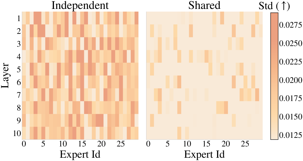
To understand why deeper recurrence fails to pay off, we investigate the root causes of this limitation and identify two main obstacles to scaling looped MoE. First, looping amplifies the curse of depth Sun et al. (2025): repeatedly reusing shared Transformer blocks causes residual accumulation and activation variance growth, as shown in Figure 3, which makes hidden states drift and destabilizes optimization in deep recurrence. Second, looped MoE suffers from expert selection collapse: shared routers produce nearly invariant expert assignments across loops, so later iterations repeatedly activate similar experts instead of refining earlier representations (shown in Figure 4). As a result, increasing loop depth adds computation without adding useful computation. This reveals the central challenge of deep looped MoE:

To answer this question, we propose LOOM, built on a single principle: each loop should contribute new computation while keeping the recurrent state stable. LOOM realizes this principle along two complementary axes, each targeting one of the obstacles identified above.

Diversifying recurrence. To counter expert selection collapse, LOOM equips each loop with its own router, so that different iterations engage different subsets of experts rather than repeatedly activating the same ones. To make these diverse computations build on one another, LOOM further introduces a Looping Residual, which carries the outputs of earlier loops forward so that later iterations can refine previous representations rather than overwrite them.

Stabilizing recurrence. To counter the curse of depth, LOOM adopts residual scaling (Sun et al., 2025; Noci et al., 2022; Wang et al., 2026a), scaling the output of each attention and MoE block by $\gamma=\lambda/(H\sqrt{M})$ . This bounds residual accumulation and keeps signal propagation stable as the number of loops grows. In addition, to prevent deep recurrence from diluting input information and causing latent drift, LOOM re-injects the input embedding at each iteration (Geiping et al., 2025). To adapt this technique to looped MoE, we recalibrate the injected embedding at step $t$ with $g_{t}=\lambda/(t\sqrt{M})$ , so that the anchoring signal remains well-scaled across iterations.

Together, these components enable shared experts to progressively refine representations across loops, allowing LOOM to scale recurrence well beyond two iterations without routing collapse or recurrent degradation. Our main contributions are as follows:

❶

We identify two main obstacles that prevent looped MoE from scaling beyond two iterations: the curse of depth, in which residual accumulation causes variance growth and latent drift, and expert selection collapse, in which shared routers assign nearly identical experts across loops.
❷

We propose LOOM, a principled recipe for deep looped MoE built on a single design principle: each loop should contribute new computation while keeping the recurrent state stable. LOOM stabilizes recurrence through residual scaling and embedding re-injection, and diversifies recurrence through loop-specific routers and a Looping Residual.
❸

Experiments across model scales from 100M to 1.7B parameters and up to 60B training tokens show that LOOM scales to 9–12 loops, and that the 1.7B model scales to 9 loops. Notably, under matched FLOPs, LOOM scales looping to 5 iterations while consistently achieving lower loss, providing strong evidence that recurrent depth is a genuine and compute-efficient scaling axis for MoE LLMs.

2 Related Work

Looped models. Looped LLMs reuse the same Transformer blocks along the depth axis, increasing effective depth without increasing parameter count. This idea traces back to Universal Transformer (Dehghani et al., 2018) and ALBERT (Lan et al., 2019). Recent studies demonstrate the potential of recurrent computation in dense Transformers: Geiping et al. (2025) show that test-time looping improves language models; Saunshi et al. (2025) connect recurrence with latent-space reasoning; and Fu et al. (2026), Wang et al. (2026a), and Movahedi et al. (2026) enable deeper recurrence through stabilization, residual scaling, and fixed-point formulations. HRM and TRM further explore recursive architectures for iterative reasoning (Wang et al., 2025a; Jolicoeur-Martineau, 2025). Chain-of-Experts studies iterative expert computation within each layer rather than recurrently reusing an entire shared MoE block (Wang et al., 2025b). Extending recurrent computation to sparse MoEs introduces additional challenges due to routing dynamics and cross-loop information propagation.

Stability in deep residual stacks. Deep recurrence increases effective depth but can amplify residual dynamics, causing activation instability and loss degradation. Noci et al. (2022) show that rank collapse of token representations causes vanishing gradients in Transformers and can be prevented by scaling residual branches, while Sun et al. (2025) identify the curse of depth in LLMs, where Pre-LN variance growth renders deeper layers nearly identity mappings and propose $1/(\sqrt{l})$ to scale down the residual. To address this, Mix-LN (Li et al., 2024) applies Post-LN to earlier layers and Pre-LN to deeper layers. Another line of work redesigns the residual pathway itself: mHC (Xie et al., 2025) constrains the residual mixing matrices of hyper-connections to a doubly stochastic manifold to restore the identity-mapping property and stabilize large-scale training, and Attention Residuals (Team et al., 2026) replace fixed additive accumulation with attention over earlier layer outputs, allowing each layer to selectively aggregate previous representations. Residual scaling has also been applied to recurrent models: Wang et al. (2026a) introduce a loop-aware factor $\lambda/(H\sqrt{M})$ , and Movahedi et al. (2026) combine residual scaling with inter-loop mixing. Input re-injection further alleviates representation drift (Geiping et al., 2025). These techniques lay the foundation for stabilizing deep recurrence and motivate their adaptation to looped MoE.

Looped MoE. Sparse gating enables MoE models to scale parameter capacity under limited computation, but introduces additional challenges for recurrent computation, particularly in expert routing and cross-loop information propagation (Shazeer et al., 2017; Fedus et al., 2022). Existing recurrent MoE studies have explored limited forms of recurrence. MoEUT extends Universal Transformer with MoE layers rather than stabilizing deep full-block recurrence (Csordás et al., 2024); Chain-of-Experts iterates experts within layers instead of reusing a shared MoE block (Wang et al., 2025b); SMELT studies compute-matched MoE looping and identifies two loops as best (Wang et al., 2026b). LoopMoE introduces iteration-adaptive normalization, while Lee et al. (2026) study recurrent MoE models with varying expert utilization but maintain effective depth by reducing layers as loop counts increase (Chen et al., 2026; Lee et al., 2026). These approaches demonstrate the potential of recurrent MoE, but scalable deep recurrence under a fixed architecture remains underexplored.

3 Methodology

Overview.

LOOM repeatedly applies an $M$ -layer, pre-norm MoE decoder. Each loop applies layers $\ell=1,2,\dots,M$ in order and repeats this walk for $H$ passes. The attention and expert weights are shared across loops, whereas each loop has its own routers. The resulting effective depth is $MH$ ; increasing $H$ adds router parameters but does not replicate the attention or experts. Let $x=\operatorname{Embed}(\mathrm{tokens})$ and let $h_{\ell}^{t}$ denote the residual stream after layer $\ell$ of loop $t$ , with $h_{0}^{1}=x$ . The final state $h_{M}^{H}$ is used for next-token prediction.

3.1 Stabilizing the recurrent state

Residual scaling.

Deep recurrence amplifies the curse of depth (Sun et al., 2025): correlated residual updates accumulate across loops, increasing hidden-state variance and destabilizing signal propagation. Figure 3(b,c) shows that unscaled residual accumulation leads to activation variance explosion during training and across loops, whereas residual scaling effectively controls this growth. Accordingly, LOOM incorporates residual scaling that accounts for both loop count and physical depth (Wang et al., 2026a):

\gamma=\frac{\lambda}{H\sqrt{M}},\quad\widetilde{h}_{\ell}^{t}=h_{\ell-1}^{t}+\gamma\,\mathrm{Attn}_{\ell}(\mathrm{RMS}(h_{\ell-1}^{t})),\quad h_{\ell}^{t}=\widetilde{h}_{\ell}^{t}+\gamma\,\mathrm{RMS}(\mathrm{MoE}_{\ell}^{t}(\mathrm{RMS}(\widetilde{h}_{\ell}^{t}))).

(1)

The $1/H$ factor limits residual accumulation across loops, while $1/\sqrt{M}$ controls variance growth across physical layers. LOOM fixes $\lambda=0.5$ as a non-learnable hyperparameter and applies $\gamma$ uniformly across layers and loops. Scaling the branch outputs preserves the identity path, while the additional MoE output normalization controls the magnitude of its residual contribution.

Figure 3: Effect of residual scaling and embedding re-injection on training stability in a 9-loop MoE model (

{\sim}350

M parameters,

10

B training tokens). Native (No Tech) loops the unmodified backbone without additional techniques. Only Res Scale and Only Embed Inject add residual scaling and embedding re-injection, respectively, to Native, with no other modifications. (a) Training loss. (b) Activation variance during training. (c) Activation variance across recurrent iterations.

Embedding re-injection.

Residual scaling alone substantially reduces activation variance but yields higher training loss than the complete recipe (Figure 3), indicating that variance control alone is insufficient. Deep recurrence can also dilute input information and induce representation drift (Wang et al., 2026a). To preserve access to the original token representation, LOOM re-injects the input embedding at the beginning of each loop $t\geq 2$ :

g_{t}=\frac{\lambda}{t\sqrt{M}}.\qquad h_{0}^{t}=(1-g_{t})h_{M}^{t-1}+g_{t}x,

(2)

We use the same fixed $\lambda=0.5$ as in residual scaling. Re-injection begins at $t=2$ , since $h_{0}^{1}=x$ . The decreasing coefficient $g_{t}$ places progressively greater weight on the recurrent representation, while convex mixing regulates the embedding contribution. Removing embedding re-injection from LOOM increases validation perplexity from $18.62$ to $26.05$ at $H=9$ (Table 5), supporting its complementary role in anchoring recurrent states alongside residual scaling.

Refer to caption — Figure 4: Expert routing in a 9-loop MoE model ( ${\sim}350$ M parameters), comparing loop-specific (Independent) and shared (Shared) routers. (a) Cross-loop similarity: $\cos(\bar{\mathbf{p}}_{t},\bar{\mathbf{p}}_{t\prime})$ , where $\bar{\mathbf{p}}_{t}$ is the normalized expert-load distribution averaged across layers for loop $t$ . Each cell compares two loops; higher values indicate more similar expert utilization. (b) Cross-loop variability: $\operatorname{std}_{t}(p_{\ell,t,e})$ , where $p_{\ell,t,e}$ is the normalized load of expert $e$ at layer $\ell$ in loop $t$ . Each cell measures an expert’s load variation across loops at a given layer. Loop-specific routers yield lower similarity and greater variability, indicating more diverse expert utilization.

3.2 Diversifying computation across loops

Loop-specific routers.

Deep recurrence should enable successive loops to perform complementary computations. However, sharing routers across loops can produce nearly invariant expert selections, leading to expert selection collapse and limiting the benefits of additional iterations. LOOM addresses this limitation through loop-specific routing with shared experts: each layer uses a separate router for each loop, while its expert weights remain shared. This decouples routing decisions across iterations, enabling different stages of recurrence to access different expert combinations without replicating expert parameters. Figure 4 provides two complementary observations: (i) lower cross-loop cosine similarity of expert-load distributions and (ii) greater variation in expert loads across loops. Together, these observations support more diverse expert utilization, a prerequisite for complementary computation across recurrent iterations.

Looping Residual.

Loop-specific routers diversify computation across iterations, while progressive refinement additionally requires effective reuse of earlier computations. LOOM therefore introduces a Looping Residual based on a fixed-decay exponential moving average (EMA), with two complementary memories: (i) a global memory spanning layers and loops, and (ii) a local memory aggregating attention outputs within the current loop. For layer $\ell$ in loop $t$ , let $o_{\ell}^{t}=\gamma\,\mathrm{Attn}_{\ell}(\mathrm{RMS}(h_{\ell-1}^{t}))$ denote the scaled attention output. Each memory maintains an accumulator $N_{A}$ and a normalization factor $D_{A}$ :

N_{A}\leftarrow\beta N_{A}+o_{\ell}^{t},\quad D_{A}\leftarrow\beta D_{A}+1,\quad r_{A}=\frac{N_{A}}{D_{A}},\qquad A\in\{H,L\}.

(3)

Both pairs are initialized to zero, with fixed $\beta=0.5$ . The global pair persists across the full recurrence, whereas the local pair is reset at the beginning of each loop. Normalization by $D_{A}$ yields exponentially weighted summaries that emphasize recent computations while retaining earlier contributions. Crucially, each memory stores only one accumulator tensor and one scalar, regardless of the number of loops. This recursive formulation avoids storing the output history and requires only elementwise operations per update, introducing negligible additional memory and computational overhead relative to the backbone. The summaries replace the direct attention residual update in Equation 1:

\widetilde{h}_{\ell}^{t}=h_{\ell-1}^{t}+r_{H}+r_{L}.

(4)

The global summary $r_{H}$ and local summary $r_{L}$ aggregate attention outputs across loops and within the current loop, respectively, preserving intermediate computations for recurrent refinement. The resulting state $\widetilde{h}_{\ell}^{t}$ is subsequently processed by the MoE residual update defined in Eq. \eqrefeq:gamma.

Figure 5: Effect of segmented backpropagation (

K{=}3

) on the

{\sim}350

M model, compared with backpropagation through all loops. (a) Peak NPU memory measured with a microbatch size of 1. (b) Total training times. (c) Held-out evaluation loss (solid bars) and average accuracy across seven downstream tasks (hatched bars).

3.3 Training with segmented backpropagation

LOOM uses segmented backpropagation, dividing the $H$ recurrent loops into consecutive segments of at most $K=3$ loops. Each segment receives supervision from a language-modeling loss at its final loop, with gradients restricted to that segment. The residual state and global Looping Residual memory are then propagated to the next segment with gradients detached, preserving forward information across all $H$ loops while limiting backpropagation depth.

Figure 5 compares this strategy with backpropagation through all $H$ loops on the ${\sim}350$ M model, highlighting two benefits. ❶ Lower memory consumption and faster training. From $H=3$ to $H=12$ , segmentation maintains peak memory near $12.6$ GiB, whereas unsegmented memory increases from $12.5$ to $19.3$ GiB. At $H=12$ , the reported training time decreases from $26.1$ to $12.6$ hours. ❷ Improved stability and performance. Segmented runs achieve lower evaluation loss and higher average accuracy across seven downstream tasks. At $H=9$ , the unsegmented run exhibits severe degradation, with evaluation loss reaching approximately $4.4$ and average accuracy falling to approximately $34\%$ . These benefits in speed and stability motivate using segmented backpropagation with $K{=}3$ by default in LOOM. Detailed comparisons in Table 6 further support using segmented backpropagation by default in LOOM.

Algorithm 1 Training procedure of LOOM.

\mathrm{sg}(\cdot)

stops gradient flow.

1: Loop count

H

, depth

M

, segment length

K=3

\lambda=\beta=0.5

x,h_{0}^{1}\leftarrow\mathrm{Embed}(\mathrm{tokens})

;

\gamma\leftarrow\lambda/(H\sqrt{M})

; init shared Looping Residual

(N_{H},D_{H})\leftarrow(0,0)

3: for

t=1,\dots,H

4: if

t\geq 2

then

g_{t}\leftarrow\lambda/(t\sqrt{M})

;

h_{0}^{t}\leftarrow(1-g_{t})h_{M}^{t-1}+g_{t}x

\triangleright

Formula (2)

(N_{L},D_{L})\leftarrow(0,0)

\triangleright

Reset local memory

6: for

\ell=1,\dots,M

o_{\ell}^{t}\leftarrow\gamma\,\mathrm{Attn}_{\ell}(\mathrm{RMS}(h_{\ell-1}^{t}))

; update both Looping Residual via Formula (3)

\widetilde{h}_{\ell}^{t}\leftarrow h_{\ell-1}^{t}+r_{H}+r_{L}

;

h_{\ell}^{t}\leftarrow\widetilde{h}_{\ell}^{t}+\gamma\,\mathrm{RMS}(\mathrm{MoE}_{\ell}^{t}(\mathrm{RMS}(\widetilde{h}_{\ell}^{t})))

9: if

t\bmod K=0

t=H

then

10:

\hat{y}^{t}\leftarrow\mathrm{LMHead}(\mathrm{RMS}(h_{M}^{t}))

; backward; optimizer step

11:

(h_{M}^{t},N_{H},D_{H})\leftarrow\mathrm{sg}(h_{M}^{t},N_{H},D_{H})

\triangleright

Stop gradient

Algorithm 1 summarizes the forward computation and segmented training procedure of LOOM.

4 Empirical results

In this section, we present the experimental setup (Section 4.1), loop-depth results from ${\sim}100$ M to ${\sim}1.7$ B (Section 4.2), and ablations of the recipe (Section 4.3).

4.1 Experimental setup

Table 1: Architecture and optimization settings for the three LOOM scales. Effective depth is

MH

, with an

M

-layer block reused for

H

recurrent iterations.

Parameters (activated)	${\sim}100$ M ( ${\sim}70$ M)	${\sim}350$ M ( ${\sim}141$ M)	${\sim}1.7$ B ( ${\sim}0.63$ B)
Physical layers $M$	$6$	$10$	$15$
Effective depth	$6H$	$10H$	$15H$
Hidden size $d$	$384$	$512$	$1280$
Query / KV heads	$6$ / $3$	$8$ / $4$	$20$ / $10$
Head dimension	$64$	$64$	$64$
Expert width $I$	$384$	$512$	$768$
Routed / shared experts	$24$ / $2$	$30$ / $2$	$30$ / $2$
Top- $k$	$6$ ( $4{+}2$ )	$8$ ( $6{+}2$ )	$8$ ( $6{+}2$ )
Router	per-loop sigmoid, float32	per-loop sigmoid, float32	per-loop sigmoid, float32
$z$ -loss / capacity	$10^{-3}$ / $1.5$	$10^{-3}$ / $1.5$	$10^{-3}$ / $1.5$
Load-balance bias LR	$2{\times}10^{-3}$	$2{\times}10^{-3}$	$2{\times}10^{-3}$
$\lambda/\beta/K$	$0.5/0.5/3$	$0.5/0.5/3$	$0.5/0.5/3$
Peak LR	$4{\times}10^{-4}$	$2{\times}10^{-4}$	$6{\times}10^{-5}$
Tokens	${\sim}5$ B	${\sim}10$ B	${\sim}60$ B

Models and datasets.

LOOM uses a Llama-style pre-norm decoder (Xiong et al., 2020; Touvron et al., 2023) with grouped-query attention (Ainslie et al., 2023), RoPE (Su et al., 2024) ( $\theta=10^{4}$ ), and sparse SwiGLU MoE layers (Shazeer, 2020; Dai et al., 2024; Jiang et al., 2024). Each loop applies layers $\ell=1,2,\dots,M$ in order and repeats this walk for $H$ passes. Models are pretrained on FineWeb-Edu (Penedo et al., 2024) with sequence length $1{,}024$ and a $65{,}536$ -token vocabulary. Table 1 lists the architecture and optimization settings. The ${\sim}100$ M model uses $M{=}6$ , hidden size $384$ , $24$ routed experts, and top- $k{=}6$ . The ${\sim}350$ M and ${\sim}1.7$ B models use $30$ routed experts and $2$ shared experts, with top- $k{=}8$ comprising $6$ routed and $2$ shared experts. All scales use loop-specific sigmoid routers in float32 and share the same $z$ -loss coefficient, capacity factor, and load-balancing bias learning rate. Loop-specific coefficients are fixed across scales ( $\lambda{=}0.5$ , $\beta{=}0.5$ , $K{=}3$ ); width and expert dimensions scale with model size, while these coefficients do not. Within each scale, the settings in Table 1 stay fixed when varying $H$ , so the loop-depth comparisons in Section 4.2 isolate recurrence depth.

Hyperparameters.

We train all models with AdamW (Loshchilov and Hutter, 2017) ( $\beta_{1}=0.9$ , $\beta_{2}=0.95$ , weight decay $0.1$ ), gradient clipping at $1.0$ , and a $10/80/10$ warmup–stable–decay schedule (Hu et al., 2024) with a $0.1\times$ peak learning-rate floor. The global batch is $1{,}024$ .

Baselines.

We compare LOOM with a non-looped $1{\times}$ baseline and three recurrent baselines matched in backbone, training data, and loop count. ❶ “No tech” loops the unmodified backbone without additional techniques. ❷ “Res. scale” builds on this native loop by applying only residual scaling. ❸ “Embed inject” builds on this native loop by applying only embedding re-injection.

Zero-shot commonsense reasoning.

We evaluate pretrained checkpoints with standard zero-shot prompts on seven tasks: PIQA (Bisk et al., 2019), SIQA (Sap et al., 2019), HellaSwag (Zellers et al., 2019), WinoGrande (Sakaguchi et al., 2021), ARC-c and ARC-e (Clark et al., 2018), and OBQA (Mihaylov et al., 2018). Unless noted otherwise, we report length-normalized accuracy (acc_norm) for OBQA, ARC-c, ARC-e, HellaSwag, and PIQA, and raw accuracy (acc) for WinoGrande and SIQA.

4.2 Loop-depth experiments

We evaluate loop depth under two protocols: near-iso-FLOP comparisons with a non-looped baseline (Section 4.2.1) and non-iso-FLOP sweeps with a fixed MoE layout, where effective depth and compute grow with $H$ (Section 4.2.2).

Table 2: Near-iso-FLOP comparison on the

M{=}10

E{=}80

backbone. All models have 700M parameters and are trained on 10B tokens. Per-token layer cost is

f=H(6+3k)

in units of

d^{2}

, anchored at

f_{1}=84

. Best results are bold.

Method	Loops	Eff. depth	top- $k$	$f(H,k)$	Val.ppl	OBQA	Wino	ARCC	ARCE	HSwg	SIQA	PIQA	Avg.
Baseline	$1{\times}$	$10$	$26$	$84$	$18.36$	$28.40$	$51.38$	$22.95$	$43.10$	$29.43$	$35.72$	$60.88$	$38.84$
LOOM	$2{\times}$	$20$	$12$	$84$	$17.37$	$30.60$	$49.33$	$24.32$	$44.57$	$29.98$	$34.65$	$59.58$	$39.00$
LOOM	$3{\times}$	$30$	$8$	$90$	$16.91$	$30.20$	$50.38$	$\mathbf{25.00}$	$44.02$	$30.05$	$35.18$	$60.55$	$39.34$
LOOM	$4{\times}$	$40$	$5$	$84$	$16.58$	$30.20$	$50.28$	$24.74$	$44.11$	$30.14$	$\mathbf{36.01}$	$\mathbf{61.26}$	$\mathbf{39.53}$
LOOM	$5{\times}$	$50$	$4$	$90$	$\mathbf{16.54}$	$\mathbf{30.80}$	$50.20$	$24.91$	$\mathbf{44.70}$	$\mathbf{30.46}$	$34.65$	$60.99$	$\mathbf{39.53}$
LOOM	$6{\times}$	$60$	$3$	$90$	$16.57$	$30.40$	$\mathbf{52.17}$	$24.66$	$44.02$	$29.91$	$35.16$	$60.17$	$39.50$

4.2.1 Iso-FLOP comparison

We design a near-iso-FLOP experiment to test whether a looped LOOM outperforms a non-looped one at matched compute. The backbone has $M{=}10$ layers, hidden size $d{=}512$ , expert width $I{=}d$ , and a pool of $E{=}80$ routed experts (no shared experts); we vary $H$ and shrink top- $k$ , while equivalent depth $MH$ still rises from $10$ to $60$ . These runs use full backpropagation through all loops, without segmented backpropagation; Consequently, the comparison incurs no additional LM-head evaluations or backward passes associated with segmentation. We count multiply–adds in units of $d^{2}$ per token per stacked layer. With $I{=}d$ , grouped-query $qkv$ costs $3d^{2}$ , causal SDPA costs $2d^{2}$ , and $o_{\mathrm{proj}}$ costs $1d^{2}$ , so attention is $6d^{2}$ . Each routed SwiGLU expert is three $d{\times}d$ maps and costs $3d^{2}$ ; $k$ experts therefore cost $3kd^{2}$ . Over $H$ loops the unit is

f(H,k)=H(6+3k)=3H(2+k).

(5)

We choose top- $k$ so that $f(H,k)\approx f_{1}=84$ (the non-looped anchor). Table 2 reports the compute budget of each loop count together with the experimental results. Val.ppl falls from the non-looped Baseline through Loop4, so four loops already improve on Loop2, Loop3, and Baseline (no-loop). Loop5 and Loop6 then stay with Loop4 rather than slipping. This already extends well beyond the two-loop setting adopted by prior looped models (Gao et al., 2026; Wang et al., 2026b; Lab et al., 2026).

Table 3: Non-iso-FLOP loop-depth sweeps at

{\sim}100

M and

{\sim}350

M scales, including partial stabilization baselines. We report validation perplexity (

\downarrow

) and zero-shot accuracy (%,

\uparrow

). Best results within each scale are bold;

\dagger

denotes an unrecoverable loss spike.

Model size	Method	Loops	Eff. depth	top- $k$	Val.ppl	OBQA	Wino	ARCC	ARCE	HSwg	SIQA	PIQA	Avg.
	Baseline	$1{\times}$	$6$	$6$	$26.26$	$27.20$	$48.46$	$22.95$	$40.07$	$26.85$	$34.54$	$57.02$	$36.73$
	No tech.	$3{\times}$	$18$	$6$	$27.61$	$27.80$	$48.30$	$21.93$	$38.89$	$26.24$	$34.03$	$56.96$	$36.31$
	No tech.	$6{\times}$	$36$	$6$	$1311^{\dagger}$	$27.40$	$51.54$	$24.49$	$27.53$	$25.51$	$34.90$	$48.91$	$34.33^{\dagger}$
	No tech.	$9{\times}$	$54$	$6$	$1312^{\dagger}$	$26.80$	$47.75$	$23.63$	$27.27$	$25.61$	$34.90$	$48.97$	$33.56^{\dagger}$
	No tech.	$12{\times}$	$72$	$6$	$1587^{\dagger}$	$27.20$	$49.33$	$24.06$	$28.07$	$25.34$	$34.18$	$49.51$	$33.96^{\dagger}$
	Embed inject	$3{\times}$	$18$	$6$	$27.48$	$24.80$	$52.01$	$22.27$	$37.75$	$26.21$	$33.73$	$54.68$	$35.92$
	Embed inject	$6{\times}$	$36$	$6$	$71.28^{\dagger}$	$24.60$	$49.49$	$21.84$	$32.03$	$24.79$	$34.24$	$52.72$	$34.24^{\dagger}$
	Embed inject	$9{\times}$	$54$	$6$	$141.5^{\dagger}$	$26.40$	$50.99$	$21.25$	$31.31$	$25.58$	$34.44$	$50.92$	$34.41^{\dagger}$
	Embed inject	$12{\times}$	$72$	$6$	$186.4^{\dagger}$	$25.80$	$48.86$	$22.61$	$29.84$	$25.03$	$33.67$	$51.37$	$33.88^{\dagger}$
	Res. scale	$3{\times}$	$18$	$6$	$28.99$	$26.80$	$50.12$	$23.29$	$37.46$	$26.64$	$34.29$	$56.37$	$36.42$
	Res. scale	$6{\times}$	$36$	$6$	$34.67^{\dagger}$	$25.20$	$48.62$	$25.17$	$25.88$	$25.84$	$34.14$	$48.59$	$33.35^{\dagger}$
	Res. scale	$9{\times}$	$54$	$6$	$33.78^{\dagger}$	$27.80$	$47.75$	$\mathbf{26.11}$	$26.85$	$25.42$	$32.09$	$49.89$	$33.70^{\dagger}$
	Res. scale	$12{\times}$	$72$	$6$	$35.64^{\dagger}$	$26.40$	$48.54$	$25.26$	$26.64$	$25.88$	$33.52$	$49.80$	$33.72^{\dagger}$
	LOOM	$3{\times}$	$18$	$6$	$23.21$	$28.00$	$49.49$	$24.15$	$39.81$	$27.11$	$33.21$	$57.73$	$37.07$
	LOOM	$6{\times}$	$36$	$6$	$19.81$	$29.20$	$\mathbf{54.06}$	$23.29$	$42.30$	$28.26$	$\mathbf{35.57}$	$59.90$	$38.94$
	LOOM	$9{\times}$	$54$	$6$	$19.29$	$\mathbf{31.00}$	$50.91$	$24.32$	$43.35$	$\mathbf{28.75}$	$35.26$	$\mathbf{60.17}$	$\mathbf{39.11}$
${\sim}100$ M	LOOM	$12{\times}$	$72$	$6$	$\mathbf{19.26}$	$30.80$	$50.49$	$25.17$	$\mathbf{44.23}$	$28.66$	$35.21$	$59.19$	$\mathbf{39.11}$
	Baseline	$1{\times}$	$10$	$8$	$20.07$	$28.40$	$48.54$	$23.04$	$42.42$	$28.43$	$34.80$	$60.07$	$37.96$
	No tech.	$3{\times}$	$30$	$8$	$23.75$	$27.60$	$51.54$	$22.10$	$40.07$	$26.95$	$34.75$	$56.96$	$37.14$
	No tech.	$6{\times}$	$60$	$8$	$1312^{\dagger}$	$26.80$	$49.96$	$23.89$	$27.53$	$25.62$	$35.31$	$49.24$	$34.05^{\dagger}$
	No tech.	$9{\times}$	$90$	$8$	$1313^{\dagger}$	$26.60$	$48.07$	$24.32$	$27.53$	$25.69$	$34.95$	$49.46$	$33.80^{\dagger}$
	No tech.	$12{\times}$	$120$	$8$	$1528^{\dagger}$	$27.40$	$49.41$	$23.46$	$26.92$	$25.47$	$34.29$	$48.75$	$33.67^{\dagger}$
	Embed inject	$3{\times}$	$30$	$8$	$42.76$	$26.60$	$50.99$	$20.99$	$35.27$	$26.30$	$33.52$	$54.57$	$35.46$
	Embed inject	$6{\times}$	$60$	$8$	$803.6^{\dagger}$	$29.00$	$50.67$	$24.83$	$27.82$	$25.42$	$34.60$	$49.62$	$34.57^{\dagger}$
	Embed inject	$9{\times}$	$90$	$8$	$780.6^{\dagger}$	$28.00$	$47.20$	$25.34$	$28.66$	$25.55$	$34.65$	$49.95$	$34.19^{\dagger}$
	Embed inject	$12{\times}$	$120$	$8$	$864.2^{\dagger}$	$27.60$	$49.09$	$23.98$	$29.41$	$25.21$	$33.98$	$50.28$	$34.22^{\dagger}$
	Res. scale	$3{\times}$	$30$	$8$	$23.80$	$28.40$	$50.99$	$22.44$	$40.07$	$27.26$	$34.44$	$57.56$	$37.31$
	Res. scale	$6{\times}$	$60$	$8$	$23.40$	$27.60$	$51.07$	$22.35$	$39.27$	$27.67$	$34.60$	$56.47$	$37.00$
	Res. scale	$9{\times}$	$90$	$8$	$33.89^{\dagger}$	$24.80$	$47.59$	$24.66$	$26.09$	$25.53$	$32.55$	$48.59$	$32.83^{\dagger}$
	Res. scale	$12{\times}$	$120$	$8$	$42.15^{\dagger}$	$26.20$	$50.83$	$22.18$	$34.93$	$25.76$	$34.90$	$54.90$	$35.67^{\dagger}$
	LOOM	$3{\times}$	$30$	$8$	$18.27$	$31.20$	$\mathbf{51.70}$	$24.15$	$44.19$	$29.04$	$35.11$	$60.28$	$39.38$
	LOOM	$6{\times}$	$60$	$8$	$15.35$	$32.20$	$50.43$	$26.11$	$47.98$	$31.59$	$36.13$	$61.70$	$40.88$
	LOOM	$9{\times}$	$90$	$8$	$\mathbf{14.80}$	$32.00$	$50.12$	$\mathbf{27.22}$	$47.18$	$32.41$	$\mathbf{36.90}$	$\mathbf{62.24}$	$41.15$
${\sim}350$ M	LOOM	$12{\times}$	$120$	$8$	$14.86$	$\mathbf{32.40}$	$51.14$	$26.43$	$\mathbf{48.23}$	$\mathbf{32.78}$	$36.80$	$62.13$	$\mathbf{41.42}$

4.2.2 Non-iso-FLOP loop experiments

Table 3 supports two conclusions. ❶ The complete recipe enables stable depth scaling. Across both model scales, LOOM remains stable under deeper recurrence and improves validation perplexity and downstream accuracy over the width-matched non-looped baselines. ❷ Relaxing the compute constraint favors deeper recurrence. Although performance gains gradually saturate, the highest seven-task average is attained at 12 loops in this sweep, extending beyond the preferred depth under the near-iso-FLOP setting in Section 4.2.1.

Comparisons with the three recurrent baselines further clarify the importance of the complete recipe. ❶ Native looping is insufficient. “No tech.” loops the unmodified backbone without additional techniques and rapidly becomes unstable as recurrence deepens. ❷ Residual scaling alone does not ensure stability. “Res. scale” adds only residual scaling; it mitigates perplexity degradation but still encounters unrecoverable loss spikes at larger loop counts. ❸ Embedding re-injection alone cannot sustain deep recurrence. “Embed inject” adds only embedding re-injection and exhibits substantial degradation as loop depth increases. All three underperform the non-looped baselines even at shallow recurrence, supporting the effectiveness of the combined mechanisms in LOOM for translating additional recurrent computation into performance gains.

4.2.3 Scaling Up Training

To evaluate LOOM at a larger scale, we train a ${\sim}1.7$ B-parameter model on ${\sim}60$ B tokens. Table 4 highlights two findings. ❶ Stability in large-scale training. The ${\sim}1.7$ B-parameter LOOM remains stable over ${\sim}60$ B training tokens. Nine loops perform best, at an unrolled scale of roughly $15$ B parameters ( $1.7\mathrm{B}\times 9$ ), achieving $7.77$ validation perplexity and $47.7\%$ average zero-shot accuracy. ❷ Scalability with model size. The same framework extends from ${\sim}100$ M and ${\sim}350$ M to ${\sim}1.7$ B parameters without changing its loop-specific hyperparameters, while retaining the benefits of recurrent computation. At the ${\sim}1.7$ B scale, nine loops reduce perplexity from $9.62$ to $7.77$ and improve average accuracy from $42.4\%$ to $47.7\%$ over the non-looped baseline. These results demonstrate the scalability of LOOM as MoE parameter counts increase.

Table 4: Scaling LOOM to

{\sim}1.7

B parameters and

{\sim}60

B tokens. We report validation perplexity (

\downarrow

) and zero-shot accuracy (%,

\uparrow

Method	Loops	Eff. depth	top- $k$	Val.ppl	OBQA	Wino	ARCC	ARCE	HSwg	SIQA	PIQA	Avg.
Baseline	$1{\times}$	$15$	$8$	$9.62$	$29.6$	$50.3$	$26.7$	$50.2$	$37.1$	$37.2$	$66.0$	$42.4$
LOOM	$3{\times}$	$45$	$8$	$8.94$	$31.6$	$51.3$	$27.2$	$51.0$	$39.1$	$39.1$	$68.0$	$43.9$
LOOM	$6{\times}$	$90$	$8$	$7.91$	$32.2$	$51.5$	$31.1$	$57.0$	$46.6$	$39.5$	$69.2$	$46.7$
LOOM	$9{\times}$	$135$	$8$	$\mathbf{7.77}$	$33.0$	$\mathbf{53.6}$	$\mathbf{31.7}$	$\mathbf{57.7}$	$\mathbf{48.8}$	$39.2$	$70.2$	$\mathbf{47.7}$
LOOM	$12{\times}$	$180$	$8$	$7.84$	$\mathbf{34.8}$	$50.7$	$30.5$	$56.9$	$48.6$	$\mathbf{40.0}$	$\mathbf{70.7}$	$47.5$

Table 5: Component ablation of the

{\sim}350

M LOOM model with 9 loops, evaluated at training step 5,000. Each ablated variant removes one component from the full recipe; “w/o routing refresh” uses a shared router across loops, and “w/o LR” removes the Looping Residual. The best result in each column is shown in bold.

Variant	Val.ppl	OBQA	Wino	ARCC	ARCE	HSwg	SIQA	PIQA	Avg.
LOOM	$\mathbf{18.62}$	$\mathbf{31.4}$	$51.1$	$\mathbf{26.1}$	$43.3$	$\mathbf{29.5}$	$35.8$	$61.4$	$\mathbf{39.8}$
w/o Res. scale	$24.63$	$29.2$	$50.1$	$23.8$	$42.6$	$29.4$	$35.9$	$59.4$	$38.6$
w/o Embed inject	$26.05$	$29.4$	$50.2$	$24.3$	$43.9$	$29.2$	$36.2$	$\mathbf{61.5}$	$39.2$
w/o MoE RMSNorm	$26.50$	$29.6$	$\mathbf{52.1}$	$24.1$	$43.6$	$28.7$	$35.5$	$59.4$	$39.0$
w/o Looping Residual	$19.25$	$30.8$	$49.2$	$24.2$	$\mathbf{44.8}$	$\mathbf{29.5}$	$\mathbf{36.6}$	$60.2$	$39.3$
w/o routing refresh	$19.83$	$30.0$	$51.7$	$25.4$	$43.1$	$29.4$	$35.7$	$59.2$	$39.2$

4.3 Ablation

4.3.1 Component ablation

Table 5 ablates components of the ${\sim}350$ M, 9-loop LOOM model at step 5,000, supporting two design principles. ❶ Stable recurrent states are essential for deep looping. Removing residual scaling, embedding re-injection, or MoE RMSNorm substantially increases perplexity and reduces average downstream accuracy, underscoring the need to control residual accumulation, preserve input information, and regulate activation magnitudes under repeated block reuse. ❷ Effective recurrence benefits from computational diversity and information preservation. Removing per-loop routing or the Looping Residual worsens both metrics, supporting their roles in diversifying expert computation and retaining information across iterations. Together, these results support our central claim: scaling recurrent depth requires stable hidden states and useful computation from successive loops.

4.3.2 Segmented backpropagation

LOOM adopts segmented backpropagation with segment length $K{=}3$ , detaching the hidden state between segments to restrict gradient propagation to the current segment. Table 6 shows that segmentation improves training stability, validation perplexity, and average downstream accuracy relative to full backpropagation. The comparison holds the architecture, training data, optimizer, and global batch size fixed. For the deepest full-backpropagation runs, the training micro-batch is reduced to fit the memory budget; these runs are therefore not matched to the segmented runs in activation memory. By bounding the backward graph within each segment, segmentation limits activation storage while preserving forward information across loops, supporting stable training at greater recurrence depths. These findings motivate its use as the default training strategy in the non-iso-FLOP experiments.

Table 6: Comparison of segmented backpropagation (

K{=}3

) and full backpropagation across loop depths on the

{\sim}350

M model.

Loops	Backprop	Val.ppl	OBQA	Wino	ARCC	ARCE	HSwg	SIQA	PIQA	Avg.
	$K{=}3$	$\mathbf{18.27}$	$\mathbf{31.2}$	$\mathbf{51.7}$	$\mathbf{24.2}$	$\mathbf{44.2}$	$\mathbf{29.0}$	$35.1$	$60.3$	$\mathbf{39.4}$
$3{\times}$	none	$26.63$	$29.2$	$50.2$	$23.1$	$43.7$	$28.4$	$\mathbf{35.2}$	$\mathbf{60.8}$	$38.7$
	$K{=}3$	$\mathbf{15.35}$	$\mathbf{32.2}$	$50.4$	$\mathbf{26.1}$	$\mathbf{48.0}$	$\mathbf{31.6}$	$\mathbf{36.1}$	$\mathbf{61.7}$	$\mathbf{40.9}$
$6{\times}$	none	$25.33$	$29.2$	$\mathbf{51.5}$	$24.7$	$43.2$	$29.0$	$35.7$	$60.3$	$39.1$
	$K{=}3$	$\mathbf{14.80}$	$\mathbf{32.0}$	$\mathbf{50.1}$	$\mathbf{27.2}$	$\mathbf{47.2}$	$\mathbf{32.4}$	$\mathbf{36.9}$	$\mathbf{62.2}$	$\mathbf{41.1}$
$9{\times}$	none	$81.04^{\dagger}$	$25.2$	$47.5$	$20.6$	$32.9$	$25.1$	$35.1$	$53.4$	$34.3^{\dagger}$
	$K{=}3$	$\mathbf{14.86}$	$\mathbf{32.4}$	$51.1$	$\mathbf{26.4}$	$\mathbf{48.2}$	$\mathbf{32.8}$	$\mathbf{36.8}$	$\mathbf{62.1}$	$\mathbf{41.4}$
$12{\times}$	none	$27.52$	$30.8$	$\mathbf{51.8}$	$23.0$	$43.2$	$28.3$	$35.9$	$59.8$	$39.0$

5 Conclusion

This paper presents LOOM, a scalable recipe for extending recurrent depth in MoE LLMs beyond the commonly used two-loop regime. Our analysis identifies hidden-state variance growth and expert selection collapse as key obstacles to deeper recurrence. LOOM addresses these obstacles through residual scaling and embedding re-injection to stabilize recurrent states, together with per-loop routers and a Looping Residual to diversify expert computation and preserve information across iterations. Experiments spanning approximately $100$ M to $1.7$ B parameters and up to $60$ B training tokens show stable scaling to $9$ – $12$ loops, with the $1.7$ B model scaling to $9$ loops. Under matched training FLOPs, LOOM scales to five loops while consistently achieving lower loss, providing evidence that recurrent depth offers a compute-efficient scaling axis for MoE language models.

References

Ainslie et al. (2023) J. Ainslie, J. Lee-Thorp, M. De Jong, Y. Zemlyanskiy, F. Lebrón, and S. Sanghai Gqa: training generalized multi-query transformer models from multi-head checkpoints. In Proceedings of the 2023 conference on empirical methods in natural language processing, pp. 4895–4901. Cited by: §4.1.
Bisk et al. (2019) Y. Bisk, R. Zellers, R. L. Bras, J. Gao, and Y. Choi PIQA: reasoning about physical commonsense in natural language. External Links: 1911.11641, Link Cited by: §4.1.
Chen et al. (2026) W. Chen, T. Li, W. Huang, Y. Yin, L. Shang, and C. Qin LoopMoE: unifying iterative computation with mixture-of-experts for language modeling. arXiv preprint arXiv:2606.04438. Cited by: §2.
Clark et al. (2018) P. Clark, I. Cowhey, O. Etzioni, T. Khot, A. Sabharwal, C. Schoenick, and O. Tafjord Think you have solved question answering? try arc, the ai2 reasoning challenge. arXiv preprint arXiv:1803.05457. Cited by: §4.1.
Csordás et al. (2024) R. Csordás, K. Irie, J. Schmidhuber, C. Potts, and C. D. Manning Moeut: mixture-of-experts universal transformers. Advances in Neural Information Processing Systems 37, pp. 28589–28614. Cited by: §2.
Dai et al. (2024) D. Dai, C. Deng, C. Zhao, R. Xu, H. Gao, D. Chen, J. Li, W. Zeng, X. Yu, Y. Wu, et al. Deepseekmoe: towards ultimate expert specialization in mixture-of-experts language models. In Proceedings of the 62nd annual meeting of the association for computational linguistics (volume 1: Long papers), pp. 1280–1297. Cited by: §4.1.
Dehghani et al. (2018) M. Dehghani, S. Gouws, O. Vinyals, J. Uszkoreit, and Ł. Kaiser Universal transformers. arXiv preprint arXiv:1807.03819. Cited by: §1, §2.
Fan et al. (2025) Y. Fan, Y. Du, K. Ramchandran, and K. Lee Looped transformers for length generalization. In International Conference on Learning Representations, Vol. 2025, pp. 14502–14520. Cited by: §1.
Fedus et al. (2022) W. Fedus, B. Zoph, and N. Shazeer Switch transformers: scaling to trillion parameter models with simple and efficient sparsity. Journal of Machine Learning Research 23 (120), pp. 1–39. Cited by: §1, §2.
Fu et al. (2026) R. Fu, Z. Yang, J. Zhang, J. Ma, H. Chen, Y. Li, and Y. Chang Simply stabilizing the loop via fully looped transformer. arXiv preprint arXiv:2605.18797. Cited by: §2.
Gao et al. (2026) Z. Gao, Y. Chen, Y. Xiao, X. Yang, R. Tao, J. Zhou, and B. Dai Loop the loopies!. arXiv preprint arXiv:2607.16051. Cited by: §1, §4.2.1.
Geiping et al. (2025) J. Geiping, S. McLeish, N. Jain, J. Kirchenbauer, S. Singh, B. Bartoldson, B. Kailkhura, A. Bhatele, and T. Goldstein Scaling up test-time compute with latent reasoning: a recurrent depth approach. Advances in Neural Information Processing Systems 38, pp. 41340–41391. Cited by: §1, §1, §2, §2.
Giannou et al. (2023) A. Giannou, S. Rajput, J. Sohn, K. Lee, J. D. Lee, and D. Papailiopoulos Looped transformers as programmable computers. In International Conference on Machine Learning, pp. 11398–11442. Cited by: §1.
Hao et al. (2024) S. Hao, S. Sukhbaatar, D. Su, X. Li, Z. Hu, J. Weston, and Y. Tian Training large language models to reason in a continuous latent space. arXiv preprint arXiv:2412.06769. Cited by: §1.
Hoffmann et al. (2022) J. Hoffmann, S. Borgeaud, A. Mensch, E. Buchatskaya, T. Cai, E. Rutherford, D. d. L. Casas, L. A. Hendricks, J. Welbl, A. Clark, et al. Training compute-optimal large language models. arXiv preprint arXiv:2203.15556. Cited by: §1.
Hu et al. (2024) S. Hu, Y. Tu, X. Han, C. He, G. Cui, X. Long, Z. Zheng, Y. Fang, Y. Huang, W. Zhao, et al. Minicpm: unveiling the potential of small language models with scalable training strategies. arXiv preprint arXiv:2404.06395. Cited by: §4.1.
Jiang et al. (2024) A. Q. Jiang, A. Sablayrolles, A. Roux, A. Mensch, B. Savary, C. Bamford, D. S. Chaplot, D. d. l. Casas, E. B. Hanna, F. Bressand, et al. Mixtral of experts. arXiv preprint arXiv:2401.04088. Cited by: §4.1.
Jolicoeur-Martineau (2025) A. Jolicoeur-Martineau Less is more: recursive reasoning with tiny networks. arXiv preprint arXiv:2510.04871. Cited by: §2.
Kaplan et al. (2020) J. Kaplan, S. McCandlish, T. Henighan, T. B. Brown, B. Chess, R. Child, S. Gray, A. Radford, J. Wu, and D. Amodei Scaling laws for neural language models. arXiv preprint arXiv:2001.08361. Cited by: §1.
Lab et al. (2026) N. Lab, C. Yang, C. Huang, F. Lan, H. Chen, H. Zhou, H. Song, J. Cao, J. Zhu, J. Niu, et al. Nanbeige4. 2-3b: unlocking agentic capabilities in a compact model. arXiv preprint arXiv:2607.22083. Cited by: §1, §4.2.1.
Lan et al. (2019) Z. Lan, M. Chen, S. Goodman, K. Gimpel, P. Sharma, and R. Soricut Albert: a lite bert for self-supervised learning of language representations. arXiv preprint arXiv:1909.11942. Cited by: §2.
Lee et al. (2026) R. Lee, J. Biloki, E. J. Hu, and J. May Sparse layers are critical to scaling looped language models. arXiv preprint arXiv:2605.09165. Cited by: §2.
Li et al. (2024) P. Li, L. Yin, and S. Liu Mix-ln: unleashing the power of deeper layers by combining pre-ln and post-ln. arXiv preprint arXiv:2412.13795. Cited by: §2.
Loshchilov and Hutter (2017) I. Loshchilov and F. Hutter Decoupled weight decay regularization. arXiv preprint arXiv:1711.05101. Cited by: §4.1.
Mihaylov et al. (2018) T. Mihaylov, P. Clark, T. Khot, and A. Sabharwal Can a suit of armor conduct electricity? a new dataset for open book question answering. In Proceedings of the 2018 conference on empirical methods in natural language processing, pp. 2381–2391. Cited by: §4.1.
Movahedi et al. (2026) S. Movahedi, V. Milovanović, S. L. Feigin, A. Theus, T. Hofmann, V. Boeva, T. K. Rusch, and A. Orvieto Fixed-point reasoners: stable and adaptive deep looped transformers. arXiv preprint arXiv:2606.18206. Cited by: §2, §2.
Noci et al. (2022) L. Noci, S. Anagnostidis, L. Biggio, A. Orvieto, S. P. Singh, and A. Lucchi Signal propagation in transformers: theoretical perspectives and the role of rank collapse. Advances in Neural Information Processing Systems 35, pp. 27198–27211. Cited by: §1, §2.
Penedo et al. (2024) G. Penedo, H. Kydlíček, A. Lozhkov, M. Mitchell, C. Raffel, L. Von Werra, T. Wolf, et al. The fineweb datasets: decanting the web for the finest text data at scale. Advances in Neural Information Processing Systems 37, pp. 30811–30849. Cited by: §4.1.
Sakaguchi et al. (2021) K. Sakaguchi, R. L. Bras, C. Bhagavatula, and Y. Choi Winogrande: an adversarial winograd schema challenge at scale. Communications of the ACM 64 (9), pp. 99–106. Cited by: §4.1.
Sap et al. (2019) M. Sap, H. Rashkin, D. Chen, R. Le Bras, and Y. Choi Social iqa: commonsense reasoning about social interactions. In Proceedings of the 2019 conference on empirical methods in natural language processing and the 9th international joint conference on natural language processing (EMNLP-IJCNLP), pp. 4463–4473. Cited by: §4.1.
Saunshi et al. (2025) N. Saunshi, N. Dikkala, Z. Li, S. Kumar, and S. J Reddi Reasoning with latent thoughts: on the power of looped transformers. In International Conference on Learning Representations, Vol. 2025, pp. 14855–14881. Cited by: §1, §2.
Shazeer et al. (2017) N. Shazeer, A. Mirhoseini, K. Maziarz, A. Davis, Q. Le, G. Hinton, and J. Dean Outrageously large neural networks: the sparsely-gated mixture-of-experts layer. arXiv preprint arXiv:1701.06538. Cited by: §1, §2.
Shazeer (2020) N. Shazeer Glu variants improve transformer. arXiv preprint arXiv:2002.05202. Cited by: §4.1.
Su et al. (2024) J. Su, M. Ahmed, Y. Lu, S. Pan, W. Bo, and Y. Liu Roformer: enhanced transformer with rotary position embedding. Neurocomputing 568, pp. 127063. Cited by: §4.1.
Sun et al. (2025) W. Sun, X. Song, P. Li, L. Yin, Y. Zheng, and S. Liu The curse of depth in large language models. Advances in Neural Information Processing Systems 38, pp. 163104–163136. Cited by: §1, §1, §2, §3.1.
Team et al. (2026) K. Team, G. Chen, Y. Zhang, J. Su, W. Xu, S. Pan, Y. Wang, Y. Wang, G. Chen, B. Yin, et al. Attention residuals. arXiv preprint arXiv:2603.15031. Cited by: §2.
Touvron et al. (2023) H. Touvron, T. Lavril, G. Izacard, X. Martinet, M. Lachaux, T. Lacroix, B. Rozière, N. Goyal, E. Hambro, F. Azhar, et al. Llama: open and efficient foundation language models. arXiv preprint arXiv:2302.13971. Cited by: §4.1.
Wang et al. (2025a) G. Wang, J. Li, Y. Sun, X. Chen, C. Liu, Y. Wu, M. Lu, S. Song, and Y. A. Yadkori Hierarchical reasoning model. External Links: 2506.21734, Link Cited by: §2.
Wang et al. (2026a) S. Wang, B. Li, G. Zhang, W. Huang, S. Yan, and J. Li On the residual scaling of looped transformers: stability and transferability. arXiv preprint arXiv:2606.18524. Cited by: §1, §2, §2, §3.1, §3.1.
Wang et al. (2026b) S. Wang, G. Zhang, K. Luo, Y. Wu, S. Liu, J. Liu, W. Huang, S. Yan, and J. Li SMELT: scaling laws for compute-matched moe looped transformers. arXiv preprint arXiv:2609.01343. Cited by: §1, §2, §4.2.1.
Wang et al. (2025b) Z. Wang, R. Pan, J. Yao, R. Csordas, L. Li, L. Yin, J. Wu, T. Zhang, M. Li, and S. Liu Chain-of-experts: unlocking the communication power of mixture-of-experts models. arXiv preprint arXiv:2506.18945. Cited by: §2, §2.
Xie et al. (2025) Z. Xie, Y. Wei, H. Cao, C. Zhao, C. Deng, J. Li, D. Dai, H. Gao, J. Chang, K. Yu, et al. Mhc: manifold-constrained hyper-connections. arXiv preprint arXiv:2512.24880. Cited by: §2.
Xiong et al. (2020) R. Xiong, Y. Yang, D. He, K. Zheng, S. Zheng, C. Xing, H. Zhang, Y. Lan, L. Wang, and T. Liu On layer normalization in the transformer architecture. In International conference on machine learning, pp. 10524–10533. Cited by: §4.1.
Zellers et al. (2019) R. Zellers, A. Holtzman, Y. Bisk, A. Farhadi, and Y. Choi Hellaswag: can a machine really finish your sentence?. In Proceedings of the 57th annual meeting of the association for computational linguistics, pp. 4791–4800. Cited by: §4.1.