跳到论文正文
W Papers独立论文阅读器 arXiv:2610.01109 论文正文 计算阅读时间 · 0%
引用这篇论文根据当前论文元数据生成,正式投稿前建议核对。


License: arXiv.org perpetual non-exclusive license
arXiv:2610.01109v1 [math.AP] 01 Oct 2026

Emergence of Cuspons through Wave Breaking

Yunjoo Kim and Bongsuk Kwon Address: (Yunjoo Kim) Department of Mathematical Sciences, Ulsan National Institute of Science and Technology, Ulsan, 44919, Korea Email address: gomuli3@unist.ac.kr Address: (Bongsuk Kwon) Department of Mathematical Sciences, Ulsan National Institute of Science and Technology, Ulsan, 44919, Korea Email address: bkwon@unist.ac.kr
Date: October 1, 2026
Abstract.

We study the emergence of cuspons through wave breaking, with the Camassa–Holm equation as a principal model. For a broad open class of smooth initial data, the first singularity occurs at a unique point and has the sharp local Hölder regularity C3/5\displaystyle C^{3/5}. We construct a continuation of the Lagrangian flow through this singular time and reconstruct from it a conservative Eulerian weak solution. We show that the first singularity does not simply persist after breaking; instead, it bifurcates immediately into an anticuspon–cuspon pair, each having the sharp local Hölder regularity C2/3\displaystyle C^{2/3}, with opposite one-sided slope orientations. The two singular branches move apart from the original breaking point, and the portion of the profile between them reverses its local monotonicity. The proof is based on an extended inverse-slope variable that remains regular through wave breaking. At the first singular time, this variable has a nondegenerate quadratic zero, which splits immediately afterward into two simple zeros. The corresponding degeneracy of the Lagrangian flow map converts the quadratic first-breaking geometry into the C3/5\displaystyle C^{3/5} profile and the post-breaking simple-zero geometry into the C2/3\displaystyle C^{2/3} cuspon profiles. The generalized Hunter–Saxton family provides an explicit realization of the same Lagrangian mechanism and also allows us to track the subsequent interaction and annihilation of the singular branches. Thus an anticuspon–cuspon pair emerges dynamically from smooth initial data through wave breaking, rather than being imposed through a singular traveling-wave ansatz.

1991 Mathematics Subject Classification
35B44, 35Q35, 35L67

1. Introduction

Cusped singularities arise naturally in nonlinear wave equations, often in the form of singular traveling waves or other special coherent structures. A more fundamental dynamical question is whether such profiles can be generated directly from smooth initial data. In particular, one would like to understand whether wave breaking can dynamically create cuspons, what local singularity is selected at the first breaking time, and how the resulting cusped branches evolve afterward. The purpose of this paper is to identify a mechanism by which cuspons are generated through wave breaking and to describe the associated transition in local singularity structure.

To investigate this mechanism, we first study the Camassa–Holm (CH) equation on the real line,

(1.1) ut−ux​x​t+2​γ​ux+3​u​ux=2​ux​ux​x+u​ux​x​x,x∈ℝ,u_{t}-u_{xxt}+2\gamma u_{x}+3uu_{x}=2u_{x}u_{xx}+uu_{xxx},\qquad x\in\mathbb{R},

where u=u⁡(x,t)\displaystyle u=u(x,t) is the unknown wave variable and γ≥0\displaystyle\gamma\geq 0 is the linear-dispersion parameter. Introduced by Camassa and Holm as an integrable model for unidirectional shallow-water waves, the equation is notable for its peaked solitary waves, or peakons [8]. It can also be written in the nonlocal form

ut+uux+px=0,p=(1−∂x2)−1(u2+12ux2+2γu).u_{t}+uu_{x}+p_{x}=0,\qquad p=(1-\partial_{x}^{2})^{-1}\left(u^{2}+\frac{1}{2}u_{x}^{2}+2\gamma u\right).

This formulation makes visible the competition between nonlinear transport and nonlocal forcing that underlies the singularity formation studied below.

A fundamental feature of (1.1) is wave breaking: a smooth solution may remain bounded while its slope becomes unbounded from below in finite time. Blow-up criteria and the wave-breaking mechanism have been studied extensively; see, among many works, [3, 9, 17]. The breakdown of the classical solution does not, however, terminate the dynamics. Global conservative and dissipative continuations have been constructed by passing to Lagrangian variables and adjoining quantities that remain regular when the Eulerian slope blows up [4, 5, 12]. In the case γ=0\displaystyle\gamma=0, Bressan–Chen–Zhang established uniqueness in a natural class of conservative solutions [6].

These continuation theories answer the fundamental question of whether the Camassa–Holm flow can be continued beyond wave breaking. They do not, however, determine the local Eulerian geometry generated by that continuation. In particular, they do not identify the shape of the profile immediately after the first breaking time, nor do they explain whether the post-breaking evolution dynamically selects one of the singular geometries known from special solutions. The present paper addresses this complementary geometric question: what does the conservative continuation actually look like near a generic first breaking point?

The Camassa–Holm equation admits several singular coherent structures. Lenells classified its weak traveling waves, including peakons, cuspons, stumpons, and composite waves [15]. A peakon has a corner with finite one-sided slopes, whereas a cuspon is continuous and has a vertical tangent: its derivative diverges with opposite signs on the two sides of the crest. Such solutions demonstrate that (1.1) admits cusped profiles. They arise, however, from singular traveling-wave ansatzes or other special exact constructions and therefore do not explain whether cuspons can be generated dynamically from smooth initial data through wave breaking.

A complementary line of work concerns the generic structure of singular conservative solutions. Li and Zhang identified stable local normal forms for conservative Camassa–Holm dynamics, including generic C2/3\displaystyle C^{2/3} singular curves and isolated C3/5\displaystyle C^{3/5} transition singularities [16]. Their theory describes the local regularity patterns that occur in generic conservative solutions. In our preceding work [14], we approached the problem from the formation side: for a broad open class of smooth initial data, we proved that the first wave-breaking event occurs at a unique point, is governed by a stable self-similar regime, and has the sharp local Hölder regularity C3/5\displaystyle C^{3/5}.

The present paper determines what happens next. We continue a nondegenerate first breaking point through the singular time and reconstruct the resulting Eulerian profile. The C3/5\displaystyle C^{3/5} singularity at the first breaking time does not persist as an isolated singularity. Instead, it is a transition singularity from which two distinct singular branches emerge immediately after breaking. These branches form an ordered anticuspon–cuspon pair: the left branch is a cusped local minimum and the right branch is a cusped local maximum. Each post-breaking singularity has the sharp local Hölder regularity C2/3\displaystyle C^{2/3}. The two singular branches then separate and move away from the original breaking point in opposite directions.

The bifurcation is encoded by the geometry of the extended Lagrangian variables. At the first breaking time, the extended inverse-slope variable has a nondegenerate quadratic zero at the first breaking label. Immediately afterward, this quadratic zero splits into two simple zeros. At the same time, the Lagrangian flow map degenerates quadratically at the first breaking point and linearly at each post-breaking branch. This change in degeneracy produces the transition

C3/5⟶C2/3,C^{3/5}\quad\longrightarrow\quad C^{2/3},

and determines the opposite one-sided slope orientations of the cuspon and anticuspon. Thus the post-breaking exponents and cusp geometry arise from a single Lagrangian bifurcation mechanism.

This provides a geometric refinement of both classical wave-breaking theory and conservative-solution theory. Classical results detect the loss of C1\displaystyle C^{1}-regularity through slope blow-up while the amplitude remains bounded. Conservative theories provide a continuation beyond that loss of classical regularity. Our contribution is to identify the precise local shape produced by the continuation. Near the first breaking point, the post-breaking profile is not an unspecified weak extension with unbounded slope: it has a canonical anticuspon–cuspon structure, sharp Hölder exponents, prescribed one-sided slope orientations, and a definite outward dynamics.

We construct this geometry by extending the inverse slope, the Lagrangian Jacobian, and the Lagrangian profile through the singular labels. The Eulerian solution is reconstructed only after these quantities have been continued across the degenerate set. We then prove that the reconstructed solution satisfies the derivative-energy balance law and hence defines a conservative weak solution. In the case γ=0\displaystyle\gamma=0, it belongs to the class of conservative solutions considered by Bressan–Chen–Zhang [6] and therefore agrees with the unique solution in that class. Consequently, the anticuspon–cuspon pair is not an ad hoc weak continuation or a singular profile imposed in advance; it is generated dynamically from smooth initial data by the canonical conservative evolution.

The generalized Hunter–Saxton family provides an explicit model of the same mechanism. For every positive even parameter λ\displaystyle\lambda, we derive the corresponding first-breaking and post-breaking regularity exponents. The explicit Lagrangian formulas allow the dynamics to be continued globally and make it possible to track the subsequent interaction of the cuspon and anticuspon branches. We identify a sharp criterion for their finite-time annihilation. At the collision time, two Cλ/(λ+1)\displaystyle C^{\lambda/(\lambda+1)} branches merge into a single C(2​λ−1)/(2​λ+1)\displaystyle C^{(2\lambda-1)/(2\lambda+1)} transition singularity. Thus the local birth of an anticuspon–cuspon pair and its later annihilation are two manifestations of the same degeneracy and unfolding of the Lagrangian flow map.

1.1. Main result for the Camassa–Holm equation

We consider (1.1) with initial datum u​(x,0)=u0​(x).\displaystyle u(x,0)=u_{0}(x). Let u\displaystyle u denote the corresponding classical solution on its maximal interval of classical existence, and let

ηt​(a,t)=u⁡(η⁡(a,t),t),η⁡(a,0)=a,\eta_{t}(a,t)=u(\eta(a,t),t),\qquad\eta(a,0)=a,

be the associated Lagrangian flow. Let t∗\displaystyle t_{*} denote the first breaking time. Under the generic assumptions introduced below, we will show that the first breaking occurs at an isolated Lagrangian label. To describe the local structure of the first breaking event, for each a\displaystyle a sufficiently close to a first breaking label a∗\displaystyle a_{*}, let τ⁡(a)\displaystyle\tau(a) denote the first breaking time along the characteristic issued from a\displaystyle a. The construction and regularity of τ\displaystyle\tau are established in Lemma 2.14.

Assumption 1 (Initial data and first-breaking structure).

The initial datum u0\displaystyle u_{0} is sufficiently smooth and spatially localized; for convenience, we assume that u0∈H5​(ℝ).\displaystyle u_{0}\in H^{5}(\mathbb{R}). The corresponding classical solution has a finite first breaking time t∗\displaystyle t_{*}, attained at a unique Lagrangian label a∗\displaystyle a_{*}. Moreover, the local breaking-time map τ\displaystyle\tau is C2\displaystyle C^{2} near a∗\displaystyle a_{*} and has a nondegenerate minimum there:

τ⁡(a∗)=t∗,τ′​(a∗)=0,τ′′​(a∗)>0.\tau(a_{*})=t_{*},\qquad\tau^{\prime}(a_{*})=0,\qquad\tau^{\prime\prime}(a_{*})>0.

The Sobolev index 5\displaystyle 5 is not essential and is not expected to be optimal. It is imposed only to ensure the classical regularity and the Taylor expansions required in the analysis near the first breaking time.

Assumption 1 is satisfied by the admissible class of smooth initial data constructed in [14]. The precise relation between this assumption and the sharp first-singularity structure obtained in [14] is explained in Remark 1.2.

Under the above assumptions, we obtain the following description of the first breaking event and its immediate post-breaking continuation.

Theorem 1.1 (Post-breaking cusp formation for the Camassa–Holm equation).

Suppose that Assumption 1 holds. Then the classical solution u\displaystyle u reaches its first breaking time t∗\displaystyle t_{*} at a unique Lagrangian label a∗\displaystyle a_{*}. The classical Lagrangian flow η\displaystyle\eta admits a continuation to 0≤t<t∗+ε∗\displaystyle 0\leq t<t_{*}+\varepsilon_{*} for some ε∗>0\displaystyle\varepsilon_{*}>0. The corresponding Eulerian reconstruction defines a conservative weak solution on this interval and agrees with the classical solution for 0≤t<t∗\displaystyle 0\leq t<t_{*}.

At the first breaking time, the solution develops a single singularity with exact local Hölder exponent 3/5\displaystyle 3/5. Immediately after t∗\displaystyle t_{*}, this singularity bifurcates into an anticuspon–cuspon pair, each having exact local Hölder exponent 2/3\displaystyle 2/3. More precisely, the following assertions hold.

  1. (i)

    The Lagrangian flow extends continuously to t=t∗\displaystyle t=t_{*}, and the solution loses C1\displaystyle C^{1}-regularity at precisely one Eulerian point, x∗:=η⁡(a∗,t∗).\displaystyle x_{*}:=\eta(a_{*},t_{*}). The profile has exact local Hölder exponent 3/5\displaystyle 3/5 at x∗\displaystyle x_{*}. Namely, u⁡(⋅,t∗)\displaystyle u(\cdot,t_{*}) belongs locally to C3/5\displaystyle C^{3/5} near x∗\displaystyle x_{*}, whereas u⁡(⋅,t∗)∉Cα\displaystyle u(\cdot,t_{*})\notin C^{\alpha} in any neighborhood of x∗\displaystyle x_{*} for every α>3/5\displaystyle\alpha>3/5.

  2. (ii)

    There exist two singular branches x−,x+:(t∗,t∗+ε∗)⟶ℝ\displaystyle x_{-},x_{+}:(t_{*},t_{*}+\varepsilon_{*})\longrightarrow\mathbb{R} such that

    x−​(t)<x+​(t),limt↓t∗x−​(t)=limt↓t∗x+​(t)=x∗.x_{-}(t)<x_{+}(t),\qquad\lim_{t\downarrow t_{*}}x_{-}(t)=\lim_{t\downarrow t_{*}}x_{+}(t)=x_{*}.

    For every t∈(t∗,t∗+ε∗)\displaystyle t\in(t_{*},t_{*}+\varepsilon_{*}), the singular set emerging locally from the first breaking point consists precisely of x−​(t)\displaystyle x_{-}(t) and x+​(t)\displaystyle x_{+}(t).

    At each of these points, the Eulerian profile has exact local Hölder exponent 2/3\displaystyle 2/3. More precisely, u⁡(⋅,t)\displaystyle u(\cdot,t) is locally C2/3\displaystyle C^{2/3} near x±​(t)\displaystyle x_{\pm}(t), but does not belong locally to Cα\displaystyle C^{\alpha} near either point for any α>2/3\displaystyle\alpha>2/3.

    The one-sided derivatives at x+​(t)\displaystyle x_{+}(t) satisfy

    (1.2) limx→x+​(t)−ux​(x,t)=+∞,limx→x+​(t)+ux​(x,t)=−∞,\lim_{x\to x_{+}(t)^{-}}u_{x}(x,t)=+\infty,\qquad\lim_{x\to x_{+}(t)^{+}}u_{x}(x,t)=-\infty,

    whereas those at x−​(t)\displaystyle x_{-}(t) satisfy

    (1.3) limx→x−​(t)−ux​(x,t)=−∞,limx→x−​(t)+ux​(x,t)=+∞.\lim_{x\to x_{-}(t)^{-}}u_{x}(x,t)=-\infty,\qquad\lim_{x\to x_{-}(t)^{+}}u_{x}(x,t)=+\infty.

    Consequently, the profile has an anticuspon at x−​(t)\displaystyle x_{-}(t) and a cuspon at x+​(t)\displaystyle x_{+}(t).

The post-breaking geometry described in Theorem 1.1 is illustrated schematically in Figure 1. The proof of Theorem 1.1 is given in Section 2.

Remark 1.2 (On the hypotheses).

(i) Local nature of the nondegeneracy hypothesis. The essential local hypothesis for the post-breaking bifurcation is that the first breaking label in Assumption 1 is isolated and nondegenerate. The same local argument may be applied separately near several isolated nondegenerate first-breaking labels, provided that the corresponding neighborhoods remain disjoint.

(ii) Relation with the first-singularity structure in [14]. The nondegeneracy condition on the breaking-time map τ\displaystyle\tau is the Lagrangian counterpart of the sharp first-singularity structure obtained in [14]. We define the extended inverse-slope variable Q\displaystyle Q by Q⁡(a,t)=1ux​(η​(a,t),t)\displaystyle\textstyle Q(a,t)=\frac{1}{u_{x}(\eta(a,t),t)} away from wave breaking, and extend Q\displaystyle Q continuously through the breaking set by setting Q=0\displaystyle Q=0. As shown in Corollary 2.9, the extended inverse-slope variable Q\displaystyle Q satisfies

Q⁡(a,t∗)=−14​τ′′​(a∗)​(a−a∗)2+o⁡(|a−a∗|2)Q(a,t_{*})=-\frac{1}{4}\tau^{\prime\prime}(a_{*})(a-a_{*})^{2}+o\bigl(|a-a_{*}|^{2}\bigr)

as a→a∗\displaystyle a\to a_{*}. In particular,

Q⁡(a∗,t∗)=0,Qa​(a∗,t∗)=0,Qa​a​(a∗,t∗)=−12​τ′′​(a∗).Q(a_{*},t_{*})=0,\qquad Q_{a}(a_{*},t_{*})=0,\qquad Q_{aa}(a_{*},t_{*})=-\frac{1}{2}\tau^{\prime\prime}(a_{*}).

Consequently,

τ′′(a∗)>0⟺Qa​a(a∗,t∗)<0.\tau^{\prime\prime}(a_{*})>0\quad\Longleftrightarrow\quad Q_{aa}(a_{*},t_{*})<0.

Thus, a nondegenerate minimum of the breaking-time map is equivalent to a nondegenerate quadratic maximum of the extended inverse-slope variable at the first breaking label.

This condition is satisfied by the admissible class of smooth initial data constructed in [14]. Indeed, the self-similar analysis in [14] shows that, up to the first singular time, the spatial derivative ux\displaystyle u_{x} has a unique minimum at the modulation center and that this minimum is nondegenerate. More precisely, in the self-similar variables of [14], one has Uy​(0,s)=−2,Uy​y​(0,s)=0,Uy​y​y​(0,s)>0,\displaystyle U_{y}(0,s)=-2,U_{yy}(0,s)=0,U_{yyy}(0,s)>0, and the estimates away from y=0\displaystyle y=0 imply Uy​(y,s)>−2​ for ​y≠0.\displaystyle U_{y}(y,s)>-2\text{ for }y\neq 0. Here U\displaystyle U denotes the rescaled slope profile used in the self-similar formulation of [14]. Thus the first singularity occurs at a unique spatial point and is generated by a strict nondegenerate minimum of ux\displaystyle u_{x}.

By the Eulerian–Lagrangian correspondence established above, this unique first-singularity point corresponds to a unique breaking label a∗\displaystyle a_{*}. In terms of the extended inverse-slope variable, the nondegeneracy is expressed as

Q⁡(a∗,t∗)=0,Qa​(a∗,t∗)=0,Qa​a​(a∗,t∗)<0.Q(a_{*},t_{*})=0,\qquad Q_{a}(a_{*},t_{*})=0,\qquad Q_{aa}(a_{*},t_{*})<0.

Using Corollary 2.9, this is equivalent to

τ′​(a∗)=0,τ′′​(a∗)>0.\tau^{\prime}(a_{*})=0,\qquad\tau^{\prime\prime}(a_{*})>0.

Therefore, Assumption 1 is satisfied by the open class of smooth initial data constructed in [14], rather than only by specially tuned examples. This is precisely the Lagrangian counterpart of the sharp C3/5\displaystyle C^{3/5} first-singularity structure obtained in [14].

(iii) Finite-time breaking. The requirement t∗<∞\displaystyle t_{*}<\infty in Assumption 1 is guaranteed, for example, by the condition

u0′​(a0)<−2​K,K:=32​‖u0‖H12+3​|γ|​‖u0‖H1.u_{0}^{\prime}(a_{0})<-\sqrt{2K},\qquad K:=\frac{3}{2}\|u_{0}\|_{H^{1}}^{2}+3|\gamma|\|u_{0}\|_{H^{1}}.

This condition is used only to guarantee finite-time wave breaking and may be replaced by any other standard wave-breaking criterion. By itself, however, it does not imply that the first breaking label is unique or that the breaking-time map has a nondegenerate minimum. A proof of this sufficient criterion is given in Proposition 2.3.

Remark 1.3 (Identification with the canonical conservative solution).

For the case of γ=0\displaystyle\gamma=0 in (1.1), the Eulerian solution produced by the post-breaking Lagrangian construction belongs to the conservative solution class specified in Section 2.6 following [6]. The identification argument given there shows that this continuation agrees with the canonical conservative Camassa–Holm solution.

Theorem 1.1 gives a dynamical refinement of the first-singularity result in [14]. At t=t∗\displaystyle t=t_{*}, the profile has the sharp pre-shock-type Hölder exponent 3/5\displaystyle 3/5. Although this singularity is cusp-like in its Hölder scaling, it does not yet have the one-sided slope structure of either a cuspon or an anticuspon described in (1.2)–(1.3). Immediately after the breaking time, the singular point bifurcates into a C2/3\displaystyle C^{2/3} anticuspon and a C2/3\displaystyle C^{2/3} cuspon, respectively located at x−​(t)\displaystyle x_{-}(t) and x+​(t)\displaystyle x_{+}(t). The one-sided limits identify not only the strength of these singularities but also their distinct slope configurations, which become important in the interaction analysis developed below.

Refer to caption
Figure 1. Schematic illustration of the post-breaking cusp formation described in Theorem 1.1. (a) At the first breaking time t=t∗\displaystyle t=t_{*}, the Eulerian profile develops a single transition singularity at x∗\displaystyle x_{*}, with exact local Hölder exponent 3/5\displaystyle 3/5. (b) For t>t∗\displaystyle t>t_{*}, this singularity bifurcates into an anticuspon at x−​(t)\displaystyle x_{-}(t) and a cuspon at x+​(t)\displaystyle x_{+}(t), each having exact local Hölder exponent 2/3\displaystyle 2/3. (c) The corresponding singular set in the (t,x)\displaystyle(t,x)-plane. The two branches x=x−​(t)\displaystyle x=x_{-}(t) and x=x+​(t)\displaystyle x=x_{+}(t) emanate from the first breaking point (t∗,x∗)\displaystyle(t_{*},x_{*}). The figure is schematic and is not drawn to scale.

To isolate the underlying Lagrangian mechanism from the specific nonlocal structure of the Camassa–Holm equation, we also study the generalized Hunter–Saxton family, for which the same bifurcation mechanism becomes explicit.

1.2. The generalized Hunter–Saxton family

The generalized Hunter–Saxton family is given by

(1.4) vt​x+v​vx​x=−1λ​vx2,λ∈2​ℕ={2,4,6,…}.v_{tx}+vv_{xx}=-\frac{1}{\lambda}v_{x}^{2},\qquad\lambda\in 2\mathbb{N}=\{2,4,6,\ldots\}.

The standard Hunter–Saxton equation corresponds to λ=2\displaystyle\lambda=2 and was introduced as an asymptotic model for director-field dynamics [13]. Generic regularity and Lipschitz metrics for conservative solutions of Hunter–Saxton type equations were studied in [7]; see also [10, 11] for further results on the regularity and uniqueness of conservative solutions.

The restriction to even λ\displaystyle\lambda is essential for our continuation mechanism. Indeed, the Jacobian of the extended Lagrangian flow is the λ\displaystyle\lambda-th power of a quantity that changes sign at breaking. Consequently, the extended flow remains monotone after its Jacobian vanishes, allowing one to recover a single-valued Eulerian solution beyond the first singular time.

For a classical solution v\displaystyle v of (1.4), let

ζt​(a,t)=v⁡(ζ⁡(a,t),t),ζ⁡(a,0)=a,\zeta_{t}(a,t)=v(\zeta(a,t),t),\qquad\zeta(a,0)=a,

denote the associated Lagrangian flow. It is convenient to introduce the degeneracy factor

DHS​(a,t):=1+tλ​v0′​(a).D_{\mathrm{HS}}(a,t):=1+\frac{t}{\lambda}v_{0}^{\prime}(a).

As shown below, the singular labels are precisely the zeros of DHS\displaystyle D_{\mathrm{HS}}.

Assumption 2 (Initial data and first-breaking structure).

The initial datum satisfies the following conditions.

  1. (H1)

    The initial profile is smooth and its derivative satisfies

    v0∈C∞​(ℝ),v0′∈L1​(ℝ)∩Lλ​(ℝ).v_{0}\in C^{\infty}(\mathbb{R}),\qquad v_{0}^{\prime}\in L^{1}(\mathbb{R})\cap L^{\lambda}(\mathbb{R}).
  2. (H2)

    The initial slope v0′\displaystyle v_{0}^{\prime} attains a unique nondegenerate negative minimum at a label a0\displaystyle a_{0}:

    v0′​(a0)=mina∈ℝ⁡v0′​(a)<0,v0′′​(a0)=0,v0(3)​(a0)>0.v_{0}^{\prime}(a_{0})=\min_{a\in\mathbb{R}}v_{0}^{\prime}(a)<0,\qquad v_{0}^{\prime\prime}(a_{0})=0,\qquad v_{0}^{(3)}(a_{0})>0.
  3. (H3)

    The initial slope satisfies

    v0′​(a)→0as ​|a|→∞.v_{0}^{\prime}(a)\rightarrow 0\qquad\text{as }|a|\to\infty.

The decay condition (H3) ensures that the far-field slope remains separated from the distinguished negative minimum v0′​(a0)\displaystyle v_{0}^{\prime}(a_{0}), so that the first-breaking structure is localized near a0\displaystyle a_{0}.

In both the Camassa–Holm and generalized Hunter–Saxton settings, we use the notation a±​(t)\displaystyle a_{\pm}(t) for the two post-breaking singular labels and x±​(t)\displaystyle x_{\pm}(t) for their corresponding Eulerian cusp locations. Since the two equations are treated separately, no confusion should arise.

Theorem 1.4 (Post-breaking cusp formation for the generalized Hunter–Saxton equation).

Suppose that Assumption 2 holds. Then the first singular time is t∗=−λv0′​(a0),\displaystyle\textstyle t_{*}=-\frac{\lambda}{v_{0}^{\prime}(a_{0})}, and the first breaking occurs at the unique Lagrangian label a0\displaystyle a_{0}.

There exists εHS>0\displaystyle\varepsilon_{\mathrm{HS}}>0 such that the classical Lagrangian flow admits a continuation to 0≤t<t∗+εHS\displaystyle 0\leq t<t_{*}+\varepsilon_{\mathrm{HS}}. The corresponding Eulerian reconstruction defines a continuous function

v:ℝ×[0,t∗+εHS)⟶ℝ,v(⋅,0)=v0,v:\mathbb{R}\times[0,t_{*}+\varepsilon_{\mathrm{HS}})\longrightarrow\mathbb{R},\qquad v(\cdot,0)=v_{0},

such that, for every T<t∗+εHS\displaystyle T<t_{*}+\varepsilon_{\mathrm{HS}}, v\displaystyle v is an Eulerian weak solution of (1.4) on ℝ×(0,T)\displaystyle\mathbb{R}\times(0,T).

Moreover, the exact conservation law

(1.5) ‖vx​(⋅,t)‖Lλ​(ℝ)=‖v0′‖Lλ​(ℝ)\|v_{x}(\cdot,t)\|_{L^{\lambda}(\mathbb{R})}=\|v_{0}^{\prime}\|_{L^{\lambda}(\mathbb{R})}

holds for every 0≤t<t∗+εHS\displaystyle 0\leq t<t_{*}+\varepsilon_{\mathrm{HS}}. In particular,

(1.6) vx∈L∞(0,t∗+εHS;Lλ(ℝ)),v∈Lloc∞(ℝ×[0,t∗+εHS)).v_{x}\in L^{\infty}\bigl(0,t_{*}+\varepsilon_{\mathrm{HS}};L^{\lambda}(\mathbb{R})\bigr),\qquad v\in L^{\infty}_{\mathrm{loc}}\bigl(\mathbb{R}\times[0,t_{*}+\varepsilon_{\mathrm{HS}})\bigr).

The local singularity structure is described as follows.

  1. (i)

    At the first singular time t=t∗\displaystyle t=t_{*}, the solution loses C1\displaystyle C^{1}-regularity at precisely one Eulerian point x∗:=ζ⁡(a0,t∗)\displaystyle x_{*}:=\zeta(a_{0},t_{*}). The pointwise Hölder exponent of v⁡(⋅,t∗)\displaystyle v(\cdot,t_{*}) at x∗\displaystyle x_{*} is exactly 2​λ−12​λ+1.\displaystyle\textstyle\frac{2\lambda-1}{2\lambda+1}. More precisely,

    0<limx→x∗|v⁡(x,t∗)−v⁡(x∗,t∗)||x−x∗|2​λ−12​λ+1<∞.0<\lim_{x\to x_{*}}\frac{|v(x,t_{*})-v(x_{*},t_{*})|}{|x-x_{*}|^{\frac{2\lambda-1}{2\lambda+1}}}<\infty.

    In particular, v⁡(⋅,t∗)∈C2​λ−12​λ+1\displaystyle v(\cdot,t_{*})\in C^{\frac{2\lambda-1}{2\lambda+1}} locally near x∗\displaystyle x_{*}, and this exponent is sharp.

  2. (ii)

    For every t∈(t∗,t∗+εHS)\displaystyle t\in(t_{*},t_{*}+\varepsilon_{\mathrm{HS}}), there exist exactly two singular labels near a0\displaystyle a_{0}, a−​(t)<a0<a+​(t),\displaystyle a_{-}(t)<a_{0}<a_{+}(t), satisfying DHS​(a±​(t),t)=0\displaystyle D_{\mathrm{HS}}(a_{\pm}(t),t)=0. They bifurcate from a0\displaystyle a_{0} in the sense that a±​(t)→a0\displaystyle a_{\pm}(t)\to a_{0} as t↓t∗\displaystyle t\downarrow t_{*}.

    Their Eulerian images x±​(t):=ζ⁡(a±​(t),t)\displaystyle x_{\pm}(t):=\zeta(a_{\pm}(t),t) satisfy

    x−​(t)<x+​(t),x±​(t)⟶x∗as ​t↓t∗.x_{-}(t)<x_{+}(t),\qquad x_{\pm}(t)\longrightarrow x_{*}\quad\text{as }t\downarrow t_{*}.

    Thus the single first-breaking singularity bifurcates into a pair of post-breaking singularities.

    At each x±​(t)\displaystyle x_{\pm}(t), the pointwise Hölder exponent of v⁡(⋅,t)\displaystyle v(\cdot,t) is exactly λλ+1.\displaystyle\textstyle\frac{\lambda}{\lambda+1}. More precisely,

    0<limx→x±​(t)|v⁡(x,t)−v⁡(x±​(t),t)||x−x±​(t)|λλ+1<∞.0<\lim_{x\to x_{\pm}(t)}\frac{|v(x,t)-v(x_{\pm}(t),t)|}{|x-x_{\pm}(t)|^{\frac{\lambda}{\lambda+1}}}<\infty.

    In particular, v⁡(⋅,t)∈Cλλ+1\displaystyle v(\cdot,t)\in C^{\frac{\lambda}{\lambda+1}} locally near x±​(t)\displaystyle x_{\pm}(t), and this exponent is sharp.

    The one-sided slopes satisfy

    limx→x+​(t)−vx​(x,t)=+∞,limx→x+​(t)+vx​(x,t)=−∞,\lim_{x\to x_{+}(t)^{-}}v_{x}(x,t)=+\infty,\qquad\lim_{x\to x_{+}(t)^{+}}v_{x}(x,t)=-\infty,

    whereas

    limx→x−​(t)−vx​(x,t)=−∞,limx→x−​(t)+vx​(x,t)=+∞.\lim_{x\to x_{-}(t)^{-}}v_{x}(x,t)=-\infty,\qquad\lim_{x\to x_{-}(t)^{+}}v_{x}(x,t)=+\infty.

    Consequently, x+​(t)\displaystyle x_{+}(t) is a cuspon of local-maximum type, whereas x−​(t)\displaystyle x_{-}(t) is an anticuspon of local-minimum type.

  3. (iii)

    For every t∈(t∗,t∗+εHS)\displaystyle t\in(t_{*},t_{*}+\varepsilon_{\mathrm{HS}}), the solution is C1\displaystyle C^{1} away from the cusp pair:

    v⁡(⋅,t)∈C1​(ℝ∖{x−​(t),x+​(t)}).v(\cdot,t)\in C^{1}\bigl(\mathbb{R}\setminus\{x_{-}(t),x_{+}(t)\}\bigr).

    Moreover, vx\displaystyle v_{x} is C1\displaystyle C^{1} in space-time away from the two singular branches, and v\displaystyle v is a classical solution of (1.4) there.

  4. (iv)

    The two cusp locations move outward from the central trajectory x0​(t):=ζ⁡(a0,t)\displaystyle x_{0}(t):=\zeta(a_{0},t). More precisely,

    x−′​(t)<x0′​(t)<x+′​(t).x_{-}^{\prime}(t)<x_{0}^{\prime}(t)<x_{+}^{\prime}(t).

We remark that λλ+1>2​λ−12​λ+1,\displaystyle\textstyle\frac{\lambda}{\lambda+1}>\frac{2\lambda-1}{2\lambda+1}, so the two post-breaking cuspons have strictly higher pointwise Hölder regularity than the profile at the first breaking time. When λ=2\displaystyle\lambda=2, the sharp exponents are 3/5\displaystyle 3/5 at the first breaking time and 2/3\displaystyle 2/3 at each post-breaking cuspon.

Remark 1.5 (On the uniqueness of the first breaking label).

The uniqueness assumption in Assumption 2(H2) is imposed only to exclude simultaneous first-breaking events. If v0′\displaystyle v_{0}^{\prime} has finitely many isolated nondegenerate global minima with the same negative value, then the local post-breaking construction and cusp-bifurcation analysis can be carried out independently near each corresponding first-breaking label, provided that the associated neighborhoods remain disjoint.

1.3. Global anticuspon–cuspon dynamics

Starting from the time extension of the pre-breaking Lagrangian flow obtained in Theorem 1.4, the simple form of (1.4) enables us to derive an explicit global-in-time representation of v\displaystyle v. This representation shows that the cuspon-pair formation described in Theorem 1.4 is not confined to the first breaking event: beyond the local time interval [0,t∗+εHS)\displaystyle[0,t_{*}+\varepsilon_{\mathrm{HS}}), further anticuspon–cuspon pairs may be generated at other nondegenerate negative local minima of v0′\displaystyle v_{0}^{\prime}. Conversely, a negative local maximum of v0′\displaystyle v_{0}^{\prime} may lead to the reverse phenomenon: an adjacent inner cuspon and anticuspon can collide and annihilate.

We impose the following global condition on the critical points of the initial slope.

Assumption 3 (Global critical-point structure).

Define

𝒜:={a∈ℝ:v0′′​(a)=0},𝒜−:={a∈𝒜:v0′​(a)<0}.\mathcal{A}:=\{a\in\mathbb{R}:\ v_{0}^{\prime\prime}(a)=0\},\qquad\mathcal{A}^{-}:=\{a\in\mathcal{A}:\ v_{0}^{\prime}(a)<0\}.

We assume the following.

  1. (G1)

    The set 𝒜−\displaystyle\mathcal{A}^{-} is locally finite.

  2. (G2)

    Every negative critical point of v0′\displaystyle v_{0}^{\prime} is nondegenerate:

    v0(3)​(a)≠0for every ​a∈𝒜−.v_{0}^{(3)}(a)\neq 0\qquad\text{for every }a\in\mathcal{A}^{-}.
Theorem 1.6 (Global anticuspon–cuspon dynamics for the generalized Hunter–Saxton equation).

Suppose that Assumptions 2 and 3 hold. Then the weak solution constructed in Theorem 1.4 extends globally in time. Moreover, the conservation law

‖vx​(⋅,t)‖Lλ​(ℝ)=‖v0′‖Lλ​(ℝ)\|v_{x}(\cdot,t)\|_{L^{\lambda}(\mathbb{R})}=\|v_{0}^{\prime}\|_{L^{\lambda}(\mathbb{R})}

holds for every t≥0\displaystyle t\geq 0.

Let a′<a′′\displaystyle a^{\prime}<a^{\prime\prime} be two consecutive nondegenerate negative local minima of v0′\displaystyle v_{0}^{\prime}, and assume that v0′\displaystyle v_{0}^{\prime} has a unique critical point a¯∈(a′,a′′)\displaystyle\bar{a}\in(a^{\prime},a^{\prime\prime}). Thus a¯\displaystyle\bar{a} is a nondegenerate local maximum, and

v0(3)​(a′)>0,v0(3)​(a¯)<0,v0(3)​(a′′)>0.v_{0}^{(3)}(a^{\prime})>0,\qquad v_{0}^{(3)}(\bar{a})<0,\qquad v_{0}^{(3)}(a^{\prime\prime})>0.

Consider the right-hand cuspon branch generated at a′\displaystyle a^{\prime} and the left-hand anticuspon branch generated at a′′\displaystyle a^{\prime\prime}. Then the following alternative holds.

  1. (i)

    If v0′​(a¯)<0,\displaystyle v_{0}^{\prime}(\bar{a})<0, then the two inner branches meet at the finite annihilation time tann:=−λv0′​(a¯).\displaystyle\textstyle t_{\mathrm{ann}}:=-\frac{\lambda}{v_{0}^{\prime}(\bar{a})}. At t=tann\displaystyle t=t_{\mathrm{ann}}, their Eulerian locations and profile values coincide, and the two singular branches coalesce into a single singular point. For times immediately after tann\displaystyle t_{\mathrm{ann}}, the two inner branches are absent; in this sense, the anticuspon–cuspon pair annihilates.

    Each incoming branch has exact local Hölder exponent λλ+1,\displaystyle\textstyle\frac{\lambda}{\lambda+1}, whereas the profile at the collision point has exact local Hölder exponent 2​λ−12​λ+1.\displaystyle\textstyle\frac{2\lambda-1}{2\lambda+1}. Thus the annihilation event produces an instantaneous loss of Eulerian Hölder regularity.

  2. (ii)

    If v0′​(a¯)≥0,\displaystyle v_{0}^{\prime}(\bar{a})\geq 0, then the two inner branches do not meet at any finite positive time. In particular, no finite-time anticuspon–cuspon annihilation occurs between the branches generated at a′\displaystyle a^{\prime} and a′′\displaystyle a^{\prime\prime}.

Thus, the sign of v0′​(a¯)\displaystyle v_{0}^{\prime}(\bar{a}) determines whether the two inner branches undergo annihilation in finite positive time.

1.4. Organization of the paper

Section 2 is devoted to the Camassa–Holm equation. In Sections 2.3–2.5, we construct the post-breaking Lagrangian continuation, prove the emergence of the anticuspon–cuspon pair, and determine the sharp local regularity. Section 2.6 verifies the Eulerian weak formulation and identifies the constructed continuation with the unique conservative solution in the class of [6], completing the proof of Theorem 1.1.

Section 3 treats the generalized Hunter–Saxton equation. We construct the post-breaking Eulerian weak solution, prove the conservation law (1.5), and establish the local cusp formation and sharp regularity asserted in Theorem 1.4. In Section 4, we extend this construction globally, analyze the interaction and annihilation of singular branches, and prove Theorem 1.6.

2. The Camassa–Holm equation

In this section, we prove Theorem 1.1. The proof is developed through a series of lemmas and propositions. We now return to the Camassa–Holm equation (1.1) on ℝ\displaystyle\mathbb{R}, supplemented with the initial condition

(2.1) u​(x,0)=u0​(x).u(x,0)=u_{0}(x).

Throughout this section, u\displaystyle u denotes the classical solution on its maximal interval of classical existence. Equation (1.1) is equivalently written as the nonlocal system

(2.2a) ut+u​ux\displaystyle\displaystyle u_{t}+uu_{x} =−px,\displaystyle\displaystyle=-p_{x},
(2.2b) p−px​x\displaystyle\displaystyle p-p_{xx} =u2+12​ux2+2​γ​u,\displaystyle\displaystyle=u^{2}+\frac{1}{2}u_{x}^{2}+2\gamma u,

where p=p⁡(x,t)\displaystyle p=p(x,t) denotes the Eulerian nonlocal potential. With

G(x):=12e−|x|,(1−∂x2)G=δ0,G(x):=\frac{1}{2}e^{-|x|},\qquad(1-\partial_{x}^{2})G=\delta_{0},

we have

(2.3) p=G∗(u2+12​ux2+2​γ​u).p=G*\left(u^{2}+\frac{1}{2}u_{x}^{2}+2\gamma u\right).

2.1. Energy conservation and bounds for the nonlocal potential

Lemma 2.1 (Conservation of the H1\displaystyle H^{1}-energy).

For every smooth solution of (1.1) for which the integrations below are justified,

(2.4) ∫ℝ(u2+ux2)​(x,t)​𝑑x=∫ℝ(u02+(u0′)2)​(x)​𝑑x\int_{\mathbb{R}}\bigl(u^{2}+u_{x}^{2}\bigr)(x,t)\,dx=\int_{\mathbb{R}}\bigl(u_{0}^{2}+(u_{0}^{\prime})^{2}\bigr)(x)\,dx

throughout the classical lifespan.

Proof.

Multiplying (1.1) by u\displaystyle u, integrating over ℝ\displaystyle\mathbb{R}, and integrating by parts, we obtain

∫ℝu​ut​𝑑x−∫ℝu​ux​x​t​𝑑x=12​dd​t​∫ℝ(u2+ux2)​𝑑x.\int_{\mathbb{R}}uu_{t}\,dx-\int_{\mathbb{R}}uu_{xxt}\,dx=\frac{1}{2}\frac{d}{dt}\int_{\mathbb{R}}\bigl(u^{2}+u_{x}^{2}\bigr)\,dx.

The remaining terms vanish:

∫ℝ2​γ​u​ux​𝑑x=0,∫ℝ3​u2​ux​𝑑x=0,\int_{\mathbb{R}}2\gamma uu_{x}\,dx=0,\qquad\int_{\mathbb{R}}3u^{2}u_{x}\,dx=0,

and

∫ℝ(2​u​ux​ux​x+u2​ux​x​x)​𝑑x=∫ℝ(u2​ux​x)x​𝑑x=0.\int_{\mathbb{R}}\left(2uu_{x}u_{xx}+u^{2}u_{xxx}\right)\,dx=\int_{\mathbb{R}}(u^{2}u_{xx})_{x}\,dx=0.

This proves (2.4). ∎

Lemma 2.2 (Bounds for the nonlocal potential).

Let u∈H1​(ℝ)\displaystyle u\in H^{1}(\mathbb{R}), and let p\displaystyle p be determined by (2.2b). Then ‖u‖L∞≤‖u‖H1\displaystyle\|u\|_{L^{\infty}}\leq\|u\|_{H^{1}}, p∈H1​(ℝ)\displaystyle p\in H^{1}(\mathbb{R}), and

(2.5) max⁡{‖p‖L∞,‖px‖L∞}≤12​‖u‖H12+|γ|​‖u‖L2.\max\bigl\{\|p\|_{L^{\infty}},\|p_{x}\|_{L^{\infty}}\bigr\}\leq\frac{1}{2}\|u\|_{H^{1}}^{2}+|\gamma|\|u\|_{L^{2}}.

Moreover,

(2.6) max⁡{‖p‖L2,‖px‖L2}≤12​‖u‖H12+2​|γ|​‖u‖L2.\max\bigl\{\|p\|_{L^{2}},\|p_{x}\|_{L^{2}}\bigr\}\leq\frac{1}{2}\|u\|_{H^{1}}^{2}+2|\gamma|\|u\|_{L^{2}}.
Proof.

By (2.3),

p=G∗(u2+12​ux2+2​γ​u),px=Gx∗(u2+12​ux2+2​γ​u).p=G*\left(u^{2}+\frac{1}{2}u_{x}^{2}+2\gamma u\right),\qquad p_{x}=G_{x}*\left(u^{2}+\frac{1}{2}u_{x}^{2}+2\gamma u\right).

Recall

‖G‖L∞=‖Gx‖L∞=12,‖G‖L2=‖Gx‖L2=12,\|G\|_{L^{\infty}}=\|G_{x}\|_{L^{\infty}}=\frac{1}{2},\qquad\|G\|_{L^{2}}=\|G_{x}\|_{L^{2}}=\frac{1}{2},
‖G‖L1=‖Gx‖L1=1,‖u2+12​ux2‖L1≤‖u‖H12.\|G\|_{L^{1}}=\|G_{x}\|_{L^{1}}=1,\qquad\left\|u^{2}+\frac{1}{2}u_{x}^{2}\right\|_{L^{1}}\leq\|u\|_{H^{1}}^{2}.

For K∈{G,Gx}\displaystyle K\in\{G,G_{x}\}, Young’s convolution inequality gives, for the L∞\displaystyle L^{\infty} bound,

‖K∗(u2+12​ux2+2​γ​u)‖L∞≤‖K‖L∞​‖u2+12​ux2‖L1+‖K‖L2​‖2​γ​u‖L2≤12​‖u‖H12+|γ|​‖u‖L2,\left\|K\ast\left(u^{2}+\frac{1}{2}u_{x}^{2}+2\gamma u\right)\right\|_{L^{\infty}}\leq\|K\|_{L^{\infty}}\left\|u^{2}+\frac{1}{2}u_{x}^{2}\right\|_{L^{1}}+\|K\|_{L^{2}}\|2\gamma u\|_{L^{2}}\leq\frac{1}{2}\|u\|_{H^{1}}^{2}+|\gamma|\|u\|_{L^{2}},

which yields (2.5). For the L2\displaystyle L^{2} bound,

‖K∗(u2+12​ux2+2​γ​u)‖L2≤‖K‖L2​‖u2+12​ux2‖L1+‖K‖L1​‖2​γ​u‖L2≤12​‖u‖H12+2​|γ|​‖u‖L2,\left\|K\ast\left(u^{2}+\frac{1}{2}u_{x}^{2}+2\gamma u\right)\right\|_{L^{2}}\leq\|K\|_{L^{2}}\left\|u^{2}+\frac{1}{2}u_{x}^{2}\right\|_{L^{1}}+\|K\|_{L^{1}}\|2\gamma u\|_{L^{2}}\leq\frac{1}{2}\|u\|_{H^{1}}^{2}+2|\gamma|\|u\|_{L^{2}},

which yields (2.6). ∎

2.2. Lagrangian slope dynamics and the inverse-slope variable

Let η\displaystyle\eta denote the Lagrangian flow of the classical solution:

(2.7) ηt​(a,t)=u⁡(η⁡(a,t),t),η⁡(a,0)=a.\eta_{t}(a,t)=u(\eta(a,t),t),\qquad\eta(a,0)=a.

We introduce the Lagrangian variables

U⁡(a,t)\displaystyle U(a,t) :=u⁡(η⁡(a,t),t),\displaystyle:=u(\eta(a,t),t),
P⁡(a,t)\displaystyle P(a,t) :=p⁡(η⁡(a,t),t),\displaystyle:=p(\eta(a,t),t),
S⁡(a,t)\displaystyle S(a,t) :=ux​(η⁡(a,t),t),\displaystyle:=u_{x}(\eta(a,t),t),
J⁡(a,t)\displaystyle J(a,t) :=ηa​(a,t).\displaystyle:=\eta_{a}(a,t).

Differentiating (2.2a) with respect to x\displaystyle x, using (2.2b), and then restricting to the flow (2.7), we obtain

(2.8) ∂tS=−12​S2+ℱ,\partial_{t}S=-\frac{1}{2}S^{2}+\mathcal{F},

where

(2.9) ℱ⁡(a,t):=U​(a,t)2+2​γ​U​(a,t)−P⁡(a,t).\mathcal{F}(a,t):=U(a,t)^{2}+2\gamma U(a,t)-P(a,t).

Also, by (2.7), the Lagrangian Jacobian satisfies

∂tJ=S​J,J⁡(a,0)=1.\partial_{t}J=SJ,\qquad J(a,0)=1.

By Lemma 2.2 and the conservation law (2.4), the forcing in (2.8) is uniformly bounded throughout the classical lifespan:

(2.10) |ℱ⁡(a,t)|≤K,K:=32​‖u0‖H12+3​|γ|​‖u0‖H1.|\mathcal{F}(a,t)|\leq K,\qquad K:=\frac{3}{2}\|u_{0}\|_{H^{1}}^{2}+3|\gamma|\|u_{0}\|_{H^{1}}.
Proposition 2.3 (A sufficient condition for finite-time wave breaking).

Let a0∈ℝ\displaystyle a_{0}\in\mathbb{R} satisfy

u0′​(a0)<−2​K,u_{0}^{\prime}(a_{0})<-\sqrt{2K},

where K\displaystyle K is defined in (2.10). Then the classical solution undergoes wave breaking in finite time. More precisely, S⁡(a0,t)\displaystyle S(a_{0},t) becomes unbounded from below no later than

Tcmp:=12​K​log⁡(u0′​(a0)−2​Ku0′​(a0)+2​K).T_{\mathrm{cmp}}:=\frac{1}{\sqrt{2K}}\log\left(\frac{u_{0}^{\prime}(a_{0})-\sqrt{2K}}{u_{0}^{\prime}(a_{0})+\sqrt{2K}}\right).
Proof.

Let g\displaystyle g solve

(2.11) g′​(t)=−12​g​(t)2+K,g⁡(0)=u0′​(a0).g^{\prime}(t)=-\frac{1}{2}g(t)^{2}+K,\qquad g(0)=u_{0}^{\prime}(a_{0}).

Since ℱ≤K\displaystyle\mathcal{F}\leq K, comparison with (2.8) gives S⁡(a0,t)≤g⁡(t)\displaystyle S(a_{0},t)\leq g(t) for as long as both quantities remain finite. Set κ:=2​K,C0:=g⁡(0)−κg⁡(0)+κ>1.\displaystyle\textstyle\kappa:=\sqrt{2K},C_{0}:=\frac{g(0)-\kappa}{g(0)+\kappa}>1. The solution of (2.11) is

g⁡(t)=κ​1+C0​e−κ​t1−C0​e−κ​t.g(t)=\kappa\frac{1+C_{0}e^{-\kappa t}}{1-C_{0}e^{-\kappa t}}.

Consequently,

g⁡(t)⟶−∞ast↗1κ​log⁡C0=Tcmp.g(t)\longrightarrow-\infty\qquad\text{as}\qquad t\nearrow\frac{1}{\kappa}\log C_{0}=T_{\mathrm{cmp}}.

It follows that S⁡(a0,t)\displaystyle S(a_{0},t), and hence ux\displaystyle u_{x}, becomes unbounded from below in finite time. ∎

Remark 2.4 (Wave-breaking criteria for the Camassa–Holm equation).

The condition in Proposition 2.3 is not meant to be optimal; it provides a simple sufficient criterion for the post-breaking analysis developed below. The wave-breaking theory for the Camassa–Holm equation is considerably more extensive. Various sufficient conditions, including local-in-space criteria, are known, as well as a necessary and sufficient characterization of finite-time wave breaking. We refer to [2, 3, 9, 18] and the references therein.

2.3. Post-breaking Lagrangian continuation

In this section, we construct solution in following steps: a regular coupled system, its local continuation, positivity and monotonicity, a regularity bootstrap, and the reconstruction of the Eulerian profile.

2.3.1. The extended coupled Lagrangian system

The Eulerian slope S\displaystyle S becomes unbounded at wave breaking, while the classical Jacobian J\displaystyle J may vanish. We therefore rewrite the dynamics in terms of Lagrangian variables that remain finite at the first singular time. For this purpose, we define

N:=S​J,M:=S2​J.N:=SJ,\qquad M:=S^{2}J.

We claim that the variables J,N,M\displaystyle J,N,M remain finite even when S\displaystyle S becomes unbounded.

It is convenient to work first with the cumulative energy variable

H⁡(a,t):=∫−∞a(U​(b,t)2​J​(b,t)+M⁡(b,t))​𝑑b.H(a,t):=\int_{-\infty}^{a}\bigl(U(b,t)^{2}J(b,t)+M(b,t)\bigr)\,db.

At t=0\displaystyle t=0,

H⁡(a,0)=∫−∞a|u0|2+|u0′|2​𝑑x.H(a,0)=\int_{-\infty}^{a}|u_{0}|^{2}+|u_{0}^{\prime}|^{2}\,dx.

Using the Green function G⁡(x)=12​e−|x|\displaystyle G(x)=\frac{1}{2}e^{-|x|}, define

(2.12) P⁡(a,t)\displaystyle\displaystyle P(a,t) :=∫ℝG⁡(η⁡(a,t)−η⁡(b,t))​[12​Ha​(b,t)+(12​U​(b,t)2+2​γ​U​(b,t))​ηa​(b,t)]​𝑑b,\displaystyle\displaystyle:=\int_{\mathbb{R}}G\bigl(\eta(a,t)-\eta(b,t)\bigr)\left[\frac{1}{2}H_{a}(b,t)+\left(\frac{1}{2}U(b,t)^{2}+2\gamma U(b,t)\right)\eta_{a}(b,t)\right]\,db,
(2.13) Π⁡(a,t)\displaystyle\displaystyle\Pi(a,t) :=∫ℝGx​(η⁡(a,t)−η⁡(b,t))​[12​Ha​(b,t)+(12​U​(b,t)2+2​γ​U​(b,t))​ηa​(b,t)]​𝑑b.\displaystyle\displaystyle:=\int_{\mathbb{R}}G_{x}\bigl(\eta(a,t)-\eta(b,t)\bigr)\left[\frac{1}{2}H_{a}(b,t)+\left(\frac{1}{2}U(b,t)^{2}+2\gamma U(b,t)\right)\eta_{a}(b,t)\right]\,db.

On the classical lifespan, one can see by (2.2b) that the change of variables x=η⁡(b,t)\displaystyle x=\eta(b,t) gives

P⁡(a,t)=p⁡(η⁡(a,t),t),Π⁡(a,t)=px​(η⁡(a,t),t).P(a,t)=p(\eta(a,t),t),\qquad\Pi(a,t)=p_{x}(\eta(a,t),t).

Recalling that

Ha=U2​J+M,Ht=U3+2​γ​U2−2​U​P,H_{a}=U^{2}J+M,\qquad H_{t}=U^{3}+2\gamma U^{2}-2UP,

and using the commutation of the a\displaystyle a- and t\displaystyle t-derivatives on the classical lifespan, we obtain

∂t(U2​J+M)=∂tHa=∂aHt=∂a(U3+2​γ​U2−2​U​P).\partial_{t}\bigl(U^{2}J+M\bigr)=\partial_{t}H_{a}=\partial_{a}H_{t}=\partial_{a}\left(U^{3}+2\gamma U^{2}-2UP\right).

Consequently, the regular variables (η,U,H)\displaystyle(\eta,U,H) satisfy

(2.14a) ηt\displaystyle\displaystyle\eta_{t} =U,\displaystyle\displaystyle=U,
(2.14b) Ut\displaystyle\displaystyle U_{t} =−Π,\displaystyle\displaystyle=-\Pi,
(2.14c) Ht\displaystyle\displaystyle H_{t} =U3+2​γ​U2−2​U​P.\displaystyle\displaystyle=U^{3}+2\gamma U^{2}-2UP.

Unlike the equations written in terms of the Eulerian slope

S=Uaηa,S=\frac{U_{a}}{\eta_{a}},

the system (2.14) contains no division by the Lagrangian Jacobian J=ηa\displaystyle J=\eta_{a}. Indeed, the nonlocal quantities P\displaystyle P and Π\displaystyle\Pi are defined directly from η\displaystyle\eta, U\displaystyle U, and H\displaystyle H. These expressions remain well-defined when J=ηa\displaystyle J=\eta_{a} vanishes. At such a label, the flow map may lose local invertibility, but the variables η\displaystyle\eta, U\displaystyle U, and H\displaystyle H, as well as the Lagrangian energy density Ha=U2​J+M,\displaystyle H_{a}=U^{2}J+M, remain finite. In particular, when J=0\displaystyle J=0, one has Ha=M,\displaystyle H_{a}=M, so the derivative energy is still recorded by H\displaystyle H, even though the Eulerian slope S=N/J\displaystyle S=N/J may become infinite. Thus (2.14) has no algebraic singularity at a breaking label. The local well-posedness and preservation of the admissible Lagrangian class are established in the next proposition.

Differentiating (2.14) with respect to a\displaystyle a, one obtains

(2.15a) Jt\displaystyle\displaystyle J_{t} =N,\displaystyle\displaystyle=N,
(2.15b) Nt\displaystyle\displaystyle N_{t} =12​M+ℱ​J,\displaystyle\displaystyle=\frac{1}{2}M+\mathcal{F}J,
(2.15c) Mt\displaystyle\displaystyle M_{t} =2​ℱ​N.\displaystyle\displaystyle=2\mathcal{F}N.

Moreover,

(2.16) N2=J​MN^{2}=JM

is preserved by the evolution, because ∂t(N2−J​M)=0.\displaystyle\partial_{t}(N^{2}-JM)=0. The initial data are

(2.17) J⁡(a,0)=1,N⁡(a,0)=u0′​(a),M⁡(a,0)=(u0′​(a))2.J(a,0)=1,\qquad N(a,0)=u_{0}^{\prime}(a),\qquad M(a,0)=\bigl(u_{0}^{\prime}(a)\bigr)^{2}.

We now introduce the inverse-slope variables in a local compressive interval I\displaystyle I containing the first breaking label and satisfying u0′​(a)≠0\displaystyle u_{0}^{\prime}(a)\neq 0 on I\displaystyle I. Once ℱ\displaystyle\mathcal{F} is known from (2.9) with the variables solving (2.14), define Q\displaystyle Q and R\displaystyle R on I\displaystyle I as the solutions of

(2.18) Qt=12−ℱ​Q2,Q⁡(a,0)=1u0′​(a),Q_{t}=\frac{1}{2}-\mathcal{F}Q^{2},\qquad Q(a,0)=\frac{1}{u_{0}^{\prime}(a)},

and

(2.19) Rt=(1+2​ℱ)​Q1+Q2​R,R⁡(a,0)=1+(u0′​(a))2.R_{t}=\bigl(1+2\mathcal{F}\bigr)\frac{Q}{1+Q^{2}}R,\qquad R(a,0)=1+\bigl(u_{0}^{\prime}(a)\bigr)^{2}.

Define

(2.20) J^:=Q2​R1+Q2,N^:=Q​R1+Q2,M^:=R1+Q2.\widehat{J}:=\frac{Q^{2}R}{1+Q^{2}},\qquad\widehat{N}:=\frac{QR}{1+Q^{2}},\qquad\widehat{M}:=\frac{R}{1+Q^{2}}.

A direct calculation shows that (J^,N^,M^)\displaystyle(\widehat{J},\widehat{N},\widehat{M}) satisfies (2.15), the compatibility relation N^2=J^​M^\displaystyle\widehat{N}^{2}=\widehat{J}\widehat{M}, and the initial data (2.17). By uniqueness for the linearized system, it follows that

J=J^,N=N^,M=M^J=\widehat{J},\qquad N=\widehat{N},\qquad M=\widehat{M}

on I\displaystyle I. In particular,

(2.21) J=Q2​R1+Q2,Ua=N=Q​R1+Q2,M=R1+Q2.J=\frac{Q^{2}R}{1+Q^{2}},\qquad U_{a}=N=\frac{QR}{1+Q^{2}},\qquad M=\frac{R}{1+Q^{2}}.

Where J>0\displaystyle J>0, these formulas agree with

Q=1S,R=(1+S2)​J.Q=\frac{1}{S},\qquad R=(1+S^{2})J.

Thus (2.18)–(2.19) provide a regular local description of the slope dynamics through Q=0\displaystyle Q=0.

2.3.2. Local continuous construction

Proposition 2.5 (Local continuous continuation).

Suppose that Assumption 1 holds. Then there exist ε∗>0\displaystyle\varepsilon_{*}>0 and an extended Lagrangian solution (η,U,H)\displaystyle(\eta,U,H) of (2.14) on 0≤t<t∗+ε∗.\displaystyle 0\leq t<t_{*}+\varepsilon_{*}. This solution agrees with the classical Lagrangian solution on 0≤t<t∗\displaystyle 0\leq t<t_{*}. Moreover, η\displaystyle\eta, U\displaystyle U, H\displaystyle H, P\displaystyle P, and Π\displaystyle\Pi are continuous in (a,t)\displaystyle(a,t), the map η⁡(⋅,t)\displaystyle\eta(\cdot,t) is nondecreasing for every t\displaystyle t, and

η⁡(⋅,t)−Id∈L∞​(ℝ)\eta(\cdot,t)-\operatorname{Id}\in L^{\infty}(\mathbb{R})

on every bounded time interval.

The differentiated variables J,N,M\displaystyle J,N,M satisfy (2.15) and the compatibility relation (2.16).

Let I\displaystyle I be a sufficiently small open interval containing the first breaking label a∗\displaystyle a_{*}, chosen so that the classical flow is compressive on I\displaystyle I before the first breaking time. Then the variables Q\displaystyle Q and R\displaystyle R, determined by (2.18)–(2.19), admit continuous extensions to I×[0,t∗+ε∗)\displaystyle I\times[0,t_{*}+\varepsilon_{*}) and satisfy (2.21).

Proof.

Set η~​(a,t):=η⁡(a,t)−a,\displaystyle\widetilde{\eta}(a,t):=\eta(a,t)-a, and introduce

V:={f∈Cb​(ℝ):fa∈L2​(ℝ)},‖f‖V:=‖f‖L∞+‖fa‖L2.V:=\left\{f\in C_{b}(\mathbb{R}):f_{a}\in L^{2}(\mathbb{R})\right\},\qquad\|f\|_{V}:=\|f\|_{L^{\infty}}+\|f_{a}\|_{L^{2}}.

We regard X⁡(t):=(η~​(⋅,t),U⁡(⋅,t),H⁡(⋅,t))\displaystyle X(t):=\bigl(\widetilde{\eta}(\cdot,t),U(\cdot,t),H(\cdot,t)\bigr) as an element of the Lagrangian state space ℰ:=V×H1​(ℝ)×V.\displaystyle\mathcal{E}:=V\times H^{1}(\mathbb{R})\times V. Here and below, η=Id+η~\displaystyle\eta=\operatorname{Id}+\widetilde{\eta} in the definitions of P\displaystyle P and Π\displaystyle\Pi.

On bounded subsets of the admissible Lagrangian class, the maps

(η~,U,H)⟼(P,Π),(\widetilde{\eta},U,H)\longmapsto(P,\Pi),

defined by (2.12)–(2.13) with η=Id+η~\displaystyle\eta=\operatorname{Id}+\widetilde{\eta}, are locally Lipschitz with respect to the topology of ℰ\displaystyle\mathcal{E}. Equivalently, on a neighborhood of each bounded subset of the admissible class, the regular Lagrangian system can be written as the Banach-space ordinary differential equation

Xt=ℱLag​(X),X_{t}=\mathcal{F}_{\mathrm{Lag}}(X),

where

ℱLag​(η~,U,H)=(U,−Π,U3+2​γ​U2−2​U​P).\mathcal{F}_{\mathrm{Lag}}(\widetilde{\eta},U,H)=\left(U,\,-\Pi,\,U^{3}+2\gamma U^{2}-2UP\right).

Hence the Picard–Lindelöf theorem yields a unique local solution.

To continue this solution through the first breaking time t∗\displaystyle t_{*}, we use the conservation of the total Lagrangian energy:

H⁡(+∞,t)=H⁡(+∞,0)=‖u0‖H12.H(+\infty,t)=H(+\infty,0)=\|u_{0}\|_{H^{1}}^{2}.

Consequently, the standard a priori estimates for the regular Lagrangian system yield uniform bounds for the state variable (η~​(⋅,t),U⁡(⋅,t),H⁡(⋅,t))\displaystyle\bigl(\widetilde{\eta}(\cdot,t),U(\cdot,t),H(\cdot,t)\bigr) in ℰ\displaystyle\mathcal{E} on every bounded time interval on which the solution exists. The corresponding estimates for the nonlocal quantities P\displaystyle P and Π\displaystyle\Pi remain controlled by the conserved energy. In particular, the vector field ℱLag\displaystyle\mathcal{F}_{\mathrm{Lag}} remains bounded and locally Lipschitz along the solution.

At the Eulerian breaking time t∗\displaystyle t_{*}, the Jacobian J=ηa\displaystyle J=\eta_{a} may vanish. However, the regular Lagrangian system (2.14) contains no division by J\displaystyle J. Thus the vanishing of J\displaystyle J produces no algebraic singularity in the regular Lagrangian variables. Moreover, the nonlocal quantities P\displaystyle P and Π\displaystyle\Pi remain controlled by the conserved energy. Therefore the standard continuation criterion for the Banach-space ordinary differential equation yields an extension of the regular Lagrangian solution to 0≤t<t∗+ε∗\displaystyle 0\leq t<t_{*}+\varepsilon_{*} for some ε∗>0\displaystyle\varepsilon_{*}>0.

For 0≤t<t∗\displaystyle 0\leq t<t_{*}, the regular Lagrangian system is obtained from the classical Eulerian solution, and η⁡(⋅,t)\displaystyle\eta(\cdot,t) is a diffeomorphism. Uniqueness of the Banach-space ordinary differential equation therefore implies that the extended variables agree with the classical Lagrangian variables on 0≤t<t∗.\displaystyle 0\leq t<t_{*}.

Differentiating (2.14) with respect to a\displaystyle a yields (2.15). Moreover, along this system,

∂t(N2−J​M)=0.\partial_{t}\bigl(N^{2}-JM\bigr)=0.

Since the initial data satisfy N​(a,0)2=J⁡(a,0)​M​(a,0)\displaystyle N(a,0)^{2}=J(a,0)M(a,0), it follows that N2=J​M\displaystyle N^{2}=JM is preserved throughout the extended lifespan. Hence the compatibility relation (2.16) holds on 0≤t<t∗+ε∗.\displaystyle 0\leq t<t_{*}+\varepsilon_{*}.

Finally, once the continuous forcing ℱ\displaystyle\mathcal{F} is known, for each fixed a∈I\displaystyle a\in I the parameter-dependent ordinary differential equations (2.18)–(2.19) have unique continuous solutions on 0≤t<t∗+ε∗.\displaystyle 0\leq t<t_{*}+\varepsilon_{*}. The algebraic variables (J^,N^,M^)\displaystyle(\widehat{J},\widehat{N},\widehat{M}) defined by (2.20) satisfy the same system (2.15) and the same initial data as (J,N,M)\displaystyle(J,N,M). By uniqueness, (J^,N^,M^)=(J,N,M),\displaystyle(\widehat{J},\widehat{N},\widehat{M})=(J,N,M), which proves (2.21). ∎

Proposition 2.5 gives a continuous post-breaking continuation. The higher spatial regularity needed for the cusp analysis will be obtained below by a separate bootstrap argument.

2.3.3. Positivity and monotonicity

Let I∗⋐I\displaystyle I_{*}\Subset I be a bounded interval containing a∗\displaystyle a_{*}, fix 0<ε0<ε∗\displaystyle 0<\varepsilon_{0}<\varepsilon_{*}, and set

𝒦:=I∗¯×[0,t∗+ε0].\mathcal{K}:=\overline{I_{*}}\times[0,t_{*}+\varepsilon_{0}].
Lemma 2.6 (Positivity and monotonicity).

The renormalized Jacobian R\displaystyle R remains strictly positive on 𝒦\displaystyle\mathcal{K}. More precisely, there exist constants cR,CR>0\displaystyle c_{R},C_{R}>0 such that

(2.22) 0<cR≤R⁡(a,t)≤CR0<c_{R}\leq R(a,t)\leq C_{R}

for all (a,t)∈𝒦\displaystyle(a,t)\in\mathcal{K}. Consequently,

J⁡(a,t)≥0,M⁡(a,t)>0,J(a,t)\geq 0,\qquad M(a,t)>0,

and

(2.23) J(a,t)=0⟺Q(a,t)=0.J(a,t)=0\quad\Longleftrightarrow\quad Q(a,t)=0.

In particular, for each fixed t\displaystyle t, the map a↦η⁡(a,t)\displaystyle a\mapsto\eta(a,t) is nondecreasing. If the zero set of Q⁡(⋅,t)\displaystyle Q(\cdot,t) contains no nontrivial interval, then η⁡(⋅,t)\displaystyle\eta(\cdot,t) is strictly increasing on I∗\displaystyle I_{*}.

Proof.

Equation (2.19) has the explicit representation

R⁡(a,t)=R⁡(a,0)​exp⁡(∫0t(1+2​ℱ​(a,s))​Q⁡(a,s)1+Q​(a,s)2​𝑑s).R(a,t)=R(a,0)\exp\left(\int_{0}^{t}\bigl(1+2\mathcal{F}(a,s)\bigr)\frac{Q(a,s)}{1+Q(a,s)^{2}}\,ds\right).

Since R⁡(a,0)=1+(u0′​(a))2>0\displaystyle R(a,0)=1+\bigl(u_{0}^{\prime}(a)\bigr)^{2}>0 and the coefficient in the exponential is bounded on 𝒦\displaystyle\mathcal{K}, the bounds (2.22) follow. The formulas (2.21) then imply

J=Q2​R1+Q2≥0,M=R1+Q2>0,J=\frac{Q^{2}R}{1+Q^{2}}\geq 0,\qquad M=\frac{R}{1+Q^{2}}>0,

as well as (2.23).

For a1<a2\displaystyle a_{1}<a_{2},

η⁡(a2,t)−η⁡(a1,t)=∫a1a2J⁡(a,t)​𝑑a≥0.\eta(a_{2},t)-\eta(a_{1},t)=\int_{a_{1}}^{a_{2}}J(a,t)\,da\geq 0.

Thus η⁡(⋅,t)\displaystyle\eta(\cdot,t) is nondecreasing. If Q\displaystyle Q does not vanish on an entire nonempty subinterval, every interval (a1,a2)\displaystyle(a_{1},a_{2}) contains a subinterval on which J>0\displaystyle J>0; hence the preceding inequality is strict. ∎

2.3.4. Regularity bootstrap

By Proposition 2.5, Lemma 2.6 and (2.21), the functions Q,R,J,N,M,η,U,P,Π\displaystyle Q,R,J,N,M,\eta,U,P,\Pi are continuous on 𝒦\displaystyle\mathcal{K}. Building on this, the next two lemmas establish higher regularity.

Lemma 2.7 (Regularity of the extended Lagrangian variables).

On the compact cylinder 𝒦\displaystyle\mathcal{K},

P,Pa,ℱ,ℱa∈C⁡(𝒦),P,P_{a},\mathcal{F},\mathcal{F}_{a}\in C(\mathcal{K}),

with

Pa​(a,t)=Π⁡(a,t)​J​(a,t)P_{a}(a,t)=\Pi(a,t)J(a,t)

and

ℱa​(a,t)=2​(U⁡(a,t)+γ)​Q⁡(a,t)​R​(a,t)1+Q​(a,t)2−Π⁡(a,t)​Q​(a,t)2​R​(a,t)1+Q​(a,t)2.\mathcal{F}_{a}(a,t)=2\bigl(U(a,t)+\gamma\bigr)\frac{Q(a,t)R(a,t)}{1+Q(a,t)^{2}}-\Pi(a,t)\frac{Q(a,t)^{2}R(a,t)}{1+Q(a,t)^{2}}.

Moreover,

Q,R,J,N,M∈C1​(𝒦),η,U∈C1​(𝒦),Q,R,J,N,M\in C^{1}(\mathcal{K}),\qquad\eta,U\in C^{1}(\mathcal{K}),

and, for each fixed t\displaystyle t,

η⁡(⋅,t),U⁡(⋅,t)∈C2​(I∗).\eta(\cdot,t),U(\cdot,t)\in C^{2}(I_{*}).

In particular, for every a0∈I∗\displaystyle a_{0}\in I_{*},

(2.24) R⁡(a,t)=R⁡(a0,t)+O⁡(|a−a0|)R(a,t)=R(a_{0},t)+O\bigl(|a-a_{0}|\bigr)

as a→a0\displaystyle a\to a_{0}, uniformly for t∈[0,t∗+ε0]\displaystyle t\in[0,t_{*}+\varepsilon_{0}].

Proof.

Differentiating (2.12) and (2.13) with respect to a\displaystyle a give

Pa=ηa​∫ℝGx​(η⁡(a,t)−η⁡(b,t))​ℰ​(b,t)​𝑑b=J​ΠP_{a}=\eta_{a}\int_{\mathbb{R}}G_{x}\bigl(\eta(a,t)-\eta(b,t)\bigr)\mathcal{E}(b,t)\,db=J\Pi

and

ℱa=2​(U+γ)​N−Π​J,\mathcal{F}_{a}=2(U+\gamma)N-\Pi J,

where

ℰ=(U2+2​γ​U)​J+12​M.\mathcal{E}=\bigl(U^{2}+2\gamma U\bigr)J+\frac{1}{2}M.

Thus Pa,ℱa\displaystyle P_{a},\mathcal{F}_{a} are continuous.

Differentiating (2.18) with respect to a\displaystyle a yields

∂tQa=−ℱa​Q2−2​ℱ​Q​Qa.\partial_{t}Q_{a}=-\mathcal{F}_{a}Q^{2}-2\mathcal{F}QQ_{a}.

Because Q⁡(⋅,0)=1/u0′\displaystyle Q(\cdot,0)=1/u_{0}^{\prime} is C1\displaystyle C^{1} on I\displaystyle I, the parameter-dependent ODE gives

Qa∈C⁡(𝒦).Q_{a}\in C(\mathcal{K}).

Equation (2.18) also gives Qt∈C⁡(𝒦)\displaystyle Q_{t}\in C(\mathcal{K}); hence Q∈C1​(𝒦)\displaystyle Q\in C^{1}(\mathcal{K}).

By (2.18), Rt=B​R\displaystyle R_{t}=BR where

B:=(1+2​ℱ)​Q1+Q2.B:=\bigl(1+2\mathcal{F}\bigr)\frac{Q}{1+Q^{2}}.

Here,

Ba=2​ℱa​Q1+Q2+(1+2​ℱ)​1−Q2(1+Q2)2​QaB_{a}=2\mathcal{F}_{a}\frac{Q}{1+Q^{2}}+\bigl(1+2\mathcal{F}\bigr)\frac{1-Q^{2}}{(1+Q^{2})^{2}}Q_{a}

is continuous, and it implies that

∂tRa=B​Ra+Ba​R\partial_{t}R_{a}=BR_{a}+B_{a}R

with C1\displaystyle C^{1} initial data, and consequently

R∈C1​(𝒦).R\in C^{1}(\mathcal{K}).

The algebraic formula (2.21) now give

J,N,M∈C1​(𝒦).J,N,M\in C^{1}(\mathcal{K}).

Since ηa=J\displaystyle\eta_{a}=J, Ua=N\displaystyle U_{a}=N, ηt=U\displaystyle\eta_{t}=U, and Ut=−Π\displaystyle U_{t}=-\Pi, the asserted regularity of η\displaystyle\eta and U\displaystyle U follows. Finally, (2.24) is an immediate consequence of the uniform boundedness of Ra\displaystyle R_{a} on 𝒦\displaystyle\mathcal{K}. ∎

Lemma 2.8 (Second spatial regularity bootstrap).

Under the assumptions of Lemma 2.7, the Lagrangian force Π\displaystyle\Pi is continuously differentiable with respect to a\displaystyle a, the forcing ℱ\displaystyle\mathcal{F} is twice continuously differentiable with respect to a\displaystyle a, and

Πa,ℱa​a,Qa​a∈C⁡(𝒦).\Pi_{a},\mathcal{F}_{aa},Q_{aa}\in C(\mathcal{K}).
Proof.

We first improve the spatial regularity of the Lagrangian nonlocal force Π\displaystyle\Pi. Fix a0∈I∗\displaystyle a_{0}\in I_{*}. Since

U⁡(a,t)−U⁡(a0,t)=∫a0aN⁡(α,t)​𝑑α,U(a,t)-U(a_{0},t)=\int_{a_{0}}^{a}N(\alpha,t)\,d\alpha,

and Nt\displaystyle N_{t} is continuous, differentiation with respect to t\displaystyle t is justified and by Ut=−Π\displaystyle U_{t}=-\Pi,

−Π⁡(a,t)+Π⁡(a0,t)=∫a0a(12​M​(α,t)+ℱ⁡(α,t)​J​(α,t))​𝑑α.-\Pi(a,t)+\Pi(a_{0},t)=\int_{a_{0}}^{a}\left(\frac{1}{2}M(\alpha,t)+\mathcal{F}(\alpha,t)J(\alpha,t)\right)\,d\alpha.

Therefore,

(2.25) Πa=−12​M−ℱ​J.\Pi_{a}=-\frac{1}{2}M-\mathcal{F}J.

Since M\displaystyle M, ℱ\displaystyle\mathcal{F}, and J\displaystyle J are continuous on 𝒦\displaystyle\mathcal{K}, it follows that

Πa∈C⁡(𝒦).\Pi_{a}\in C(\mathcal{K}).

Recall that

ℱa=2​(U+γ)​N−Π​J.\mathcal{F}_{a}=2(U+\gamma)N-\Pi J.

Differentiating with respect to a\displaystyle a, we obtain by (2.25) that

ℱa​a=2​N2+2​(U+γ)​Na−Πa​J−Π​Ja=2​N2+2​(U+γ)​Na+ℱ​J2+12​M​J−Π​Ja.\begin{split}\mathcal{F}_{aa}&=2N^{2}+2(U+\gamma)N_{a}-\Pi_{a}J-\Pi J_{a}\\ &=2N^{2}+2(U+\gamma)N_{a}+\mathcal{F}J^{2}+\frac{1}{2}MJ-\Pi J_{a}.\end{split}

Every quantity on the right-hand side is continuous on 𝒦\displaystyle\mathcal{K}, and hence

ℱa​a∈C⁡(𝒦).\mathcal{F}_{aa}\in C(\mathcal{K}).

We now differentiate (2.18) twice with respect to a\displaystyle a. The first derivative satisfies

∂tQa=−ℱa​Q2−2​ℱ​Q​Qa.\partial_{t}Q_{a}=-\mathcal{F}_{a}Q^{2}-2\mathcal{F}QQ_{a}.

Differentiating once more gives

(2.26) ∂tQa​a+2​ℱ​Q​Qa​a=−ℱa​a​Q2−4​ℱa​Q​Qa−2​ℱ​Qa2.\partial_{t}Q_{aa}+2\mathcal{F}QQ_{aa}=-\mathcal{F}_{aa}Q^{2}-4\mathcal{F}_{a}QQ_{a}-2\mathcal{F}Q_{a}^{2}.

Because I∗¯⋐I\displaystyle\overline{I_{*}}\Subset I and u0′\displaystyle u_{0}^{\prime} does not vanish on I\displaystyle I, it is bounded away from zero on I∗¯\displaystyle\overline{I_{*}}. Since u0∈H5​(ℝ)\displaystyle u_{0}\in H^{5}(\mathbb{R}), the initial inverse slope

Q⁡(a,0)=1u0′​(a)Q(a,0)=\frac{1}{u_{0}^{\prime}(a)}

belongs to C2​(I∗¯)\displaystyle C^{2}(\overline{I_{*}}). Equation (2.26) therefore yields

Qa​a∈C⁡(𝒦).Q_{aa}\in C(\mathcal{K}).

∎

Corollary 2.9 (Quadratic expansion at the first breaking point).

Under Assumption 1, one has

(2.27) Q⁡(a,t∗)=−14​τ′′​(a∗)​(a−a∗)2+o⁡(|a−a∗|2)Q(a,t_{*})=-\frac{1}{4}\tau^{\prime\prime}(a_{*})(a-a_{*})^{2}+o\bigl(|a-a_{*}|^{2}\bigr)

as a→a∗\displaystyle a\to a_{*}. Consequently,

(2.28) Qa​(a∗,t∗)=0,Qa​a​(a∗,t∗)=−12​τ′′​(a∗)<0.Q_{a}(a_{*},t_{*})=0,\qquad Q_{aa}(a_{*},t_{*})=-\frac{1}{2}\tau^{\prime\prime}(a_{*})<0.
Proof.

For a\displaystyle a near a∗\displaystyle a_{*}, the breaking-time map satisfies

Q⁡(a,τ⁡(a))=0,τ⁡(a)=t∗+12​τ′′​(a∗)​(a−a∗)2+o⁡(|a−a∗|2).Q(a,\tau(a))=0,\qquad\tau(a)=t_{*}+\frac{1}{2}\tau^{\prime\prime}(a_{*})(a-a_{*})^{2}+o\bigl(|a-a_{*}|^{2}\bigr).

Integrating (2.18) from t∗\displaystyle t_{*} to τ⁡(a)\displaystyle\tau(a), we obtain

Q⁡(a,t∗)=−12​(τ⁡(a)−t∗)+∫t∗τ⁡(a)ℱ⁡(a,s)​Q​(a,s)2​𝑑s.Q(a,t_{*})=-\frac{1}{2}\bigl(\tau(a)-t_{*}\bigr)+\int_{t_{*}}^{\tau(a)}\mathcal{F}(a,s)Q(a,s)^{2}\,ds.

Since Q⁡(a,τ⁡(a))=0\displaystyle Q(a,\tau(a))=0 and Qt\displaystyle Q_{t} is bounded in a neighborhood of (a∗,t∗)\displaystyle(a_{*},t_{*}),

|Q⁡(a,s)|≤C|τ⁡(a)−s|≤C​|τ⁡(a)−t∗||Q(a,s)|\leq C|\tau(a)-s|\leq C|\tau(a)-t_{*}|

for s\displaystyle s between t∗\displaystyle t_{*} and τ⁡(a)\displaystyle\tau(a). Hence, by the boundedness of ℱ\displaystyle\mathcal{F} in (2.10), we obtain

|∫t∗τ⁡(a)ℱ⁡(a,s)​Q​(a,s)2​𝑑s|≤C​|τ⁡(a)−t∗|3.\left|\int_{t_{*}}^{\tau(a)}\mathcal{F}(a,s)Q(a,s)^{2}\,ds\right|\leq C|\tau(a)-t_{*}|^{3}.

Since τ⁡(a)−t∗=O⁡(|a−a∗|2)\displaystyle\tau(a)-t_{*}=O(|a-a_{*}|^{2}), it follows that

∫t∗τ⁡(a)ℱ⁡(a,s)​Q​(a,s)2​𝑑s=o⁡(|a−a∗|2).\int_{t_{*}}^{\tau(a)}\mathcal{F}(a,s)Q(a,s)^{2}\,ds=o(|a-a_{*}|^{2}).

Substituting the expansion of τ\displaystyle\tau into the preceding identity therefore yields (2.27).

By Lemma 2.8, Q⁡(⋅,t∗)∈C2​(I∗¯)\displaystyle Q(\cdot,t_{*})\in C^{2}(\overline{I_{*}}). Comparing (2.27) with the second-order Taylor formula for Q⁡(⋅,t∗)\displaystyle Q(\cdot,t_{*}) at a∗\displaystyle a_{*} yields (2.28). ∎

Remark 2.10 (Strict monotonicity after the first breaking time).

By the definition of the local breaking-time map,

Q(a,t)=0⟺t=τ(a)Q(a,t)=0\quad\Longleftrightarrow\quad t=\tau(a)

near (a∗,t∗)\displaystyle(a_{*},t_{*}). Since τ′′​(a∗)>0\displaystyle\tau^{\prime\prime}(a_{*})>0 and τ∈C2\displaystyle\tau\in C^{2}, after shrinking I∗\displaystyle I_{*} if necessary, τ\displaystyle\tau is strictly convex on I∗\displaystyle I_{*}. Consequently, for every t∈[t∗,t∗+ε∗)\displaystyle t\in[t_{*},t_{*}+\varepsilon_{*}), the zero set

{a∈I∗:Q⁡(a,t)=0}={a∈I∗:τ⁡(a)=t}\{a\in I_{*}:Q(a,t)=0\}=\{a\in I_{*}:\tau(a)=t\}

contains at most two points and hence no nontrivial interval. It follows from Lemma 2.6 that η⁡(⋅,t)\displaystyle\eta(\cdot,t) is strictly increasing on I∗\displaystyle I_{*}. Thus, although J=ηa\displaystyle J=\eta_{a} may vanish at isolated breaking labels, no nontrivial Lagrangian interval collapses to a single Eulerian point.

2.3.5. Eulerian reconstruction

We now reconstruct the Eulerian velocity by means of a generalized inverse of the Lagrangian flow map.

Lemma 2.11 (Constancy on the fibers of the flow).

Fix 0≤t<t∗+ε∗.\displaystyle 0\leq t<t_{*}+\varepsilon_{*}. If a1<a2,η⁡(a1,t)=η⁡(a2,t),\displaystyle a_{1}<a_{2},\eta(a_{1},t)=\eta(a_{2},t), then U⁡(a1,t)=U⁡(a2,t).\displaystyle U(a_{1},t)=U(a_{2},t). More generally, for every x∈ℝ\displaystyle x\in\mathbb{R}, U⁡(⋅,t)\displaystyle U(\cdot,t) is constant on the fiber

η​(⋅,t)−1​({x})={a∈ℝ:η⁡(a,t)=x}.\eta(\cdot,t)^{-1}(\{x\})=\{a\in\mathbb{R}:\eta(a,t)=x\}.
Proof.

Since J=ηa≥0\displaystyle J=\eta_{a}\geq 0,

0=η⁡(a2,t)−η⁡(a1,t)=∫a1a2J⁡(a,t)​𝑑a.0=\eta(a_{2},t)-\eta(a_{1},t)=\int_{a_{1}}^{a_{2}}J(a,t)\,da.

Because J⁡(⋅,t)\displaystyle J(\cdot,t) is continuous and nonnegative, it follows that

J⁡(a,t)=0for all ​a∈[a1,a2].J(a,t)=0\qquad\text{for all }a\in[a_{1},a_{2}].

The compatibility relation (2.16) then gives

N​(a,t)2=J⁡(a,t)​M​(a,t)=0N(a,t)^{2}=J(a,t)M(a,t)=0

on [a1,a2]\displaystyle[a_{1},a_{2}]. Hence N=0\displaystyle N=0 there, and since Ua=N\displaystyle U_{a}=N, the function U⁡(⋅,t)\displaystyle U(\cdot,t) is constant on [a1,a2]\displaystyle[a_{1},a_{2}]. ∎

By Proposition 2.5, for every fixed 0≤t<t∗+ε∗,\displaystyle 0\leq t<t_{*}+\varepsilon_{*}, the map η⁡(⋅,t)\displaystyle\eta(\cdot,t) is continuous and nondecreasing. Moreover,

η⁡(⋅,t)−Id∈L∞​(ℝ),\eta(\cdot,t)-\operatorname{Id}\in L^{\infty}(\mathbb{R}),

and therefore

η⁡(a,t)⟶±∞as ​a⟶±∞.\eta(a,t)\longrightarrow\pm\infty\qquad\text{as }a\longrightarrow\pm\infty.

Thus η⁡(⋅,t)\displaystyle\eta(\cdot,t) maps ℝ\displaystyle\mathbb{R} onto ℝ\displaystyle\mathbb{R}.

For x∈ℝ\displaystyle x\in\mathbb{R}, define the generalized inverse

(2.29) ξ⁡(x,t):=sup{a∈ℝ:η⁡(a,t)≤x}.\xi(x,t):=\sup\left\{a\in\mathbb{R}:\eta(a,t)\leq x\right\}.

The set in (2.29) is nonempty and bounded above, so ξ⁡(x,t)\displaystyle\xi(x,t) is well defined. By the continuity and monotonicity of η⁡(⋅,t)\displaystyle\eta(\cdot,t),

η⁡(ξ⁡(x,t),t)=x.\eta(\xi(x,t),t)=x.

We then define the Eulerian velocity by

(2.30) u⁡(x,t):=U⁡(ξ⁡(x,t),t).u(x,t):=U(\xi(x,t),t).

If a\displaystyle a is any Lagrangian label satisfying

η⁡(a,t)=x,\eta(a,t)=x,

then a\displaystyle a and ξ⁡(x,t)\displaystyle\xi(x,t) belong to the same fiber of η⁡(⋅,t)\displaystyle\eta(\cdot,t). Lemma 2.11 therefore gives

U⁡(a,t)=U⁡(ξ⁡(x,t),t)=u⁡(x,t).U(a,t)=U(\xi(x,t),t)=u(x,t).

Consequently,

U⁡(a,t)=u⁡(η⁡(a,t),t)U(a,t)=u(\eta(a,t),t)

for every a∈ℝ\displaystyle a\in\mathbb{R} and 0≤t<t∗+ε∗\displaystyle 0\leq t<t_{*}+\varepsilon_{*}.

For each fixed t\displaystyle t, define the nonnegative Radon measure

μt:=η​(⋅,t)#​(M⁡(⋅,t)​d​a),\mu_{t}:=\eta(\cdot,t)_{\#}\bigl(M(\cdot,t)\,da\bigr),

that is, for every Borel set B⊂ℝ\displaystyle B\subset\mathbb{R},

μt​(B)=∫η​(⋅,t)−1​(B)M⁡(a,t)​𝑑a.\mu_{t}(B)=\int_{\eta(\cdot,t)^{-1}(B)}M(a,t)\,da.

Equivalently, for every bounded Borel function φ:ℝ→ℝ\displaystyle\varphi:\mathbb{R}\to\mathbb{R},

∫ℝφ⁡(x)​d​μt​(x)=∫ℝφ⁡(η⁡(a,t))​M​(a,t)​𝑑a.\int_{\mathbb{R}}\varphi(x)\,d\mu_{t}(x)=\int_{\mathbb{R}}\varphi\bigl(\eta(a,t)\bigr)M(a,t)\,da.

Here and after, d​μtac\displaystyle d\mu_{t}^{\mathrm{ac}} denotes the absolutely continuous part of d​μt\displaystyle d\mu_{t}, namely

d​μtac=d​μtd​x​d​x.d\mu_{t}^{\mathrm{ac}}=\frac{d\mu_{t}}{dx}\,dx.
Proposition 2.12 (Eulerian reconstruction).

For every T<t∗+ε∗\displaystyle T<t_{*}+\varepsilon_{*}, the function u\displaystyle u defined by (2.30) is continuous on ℝ×[0,T]\displaystyle\mathbb{R}\times[0,T]. Then

(2.31) d​μtac=ux​(x,t)2​d​x.d\mu_{t}^{\mathrm{ac}}=u_{x}(x,t)^{2}\,dx.

The potential satisfies

(2.32) P⁡(a,t)=p⁡(η⁡(a,t),t),P(a,t)=p(\eta(a,t),t),

where

(2.33) p⁡(x,t):=∫ℝG⁡(x−y)​(u​(y,t)2+2​γ​u​(y,t))​dy+12​∫ℝG⁡(x−y)​d​μt​(y).\begin{split}p(x,t)&:=\int_{\mathbb{R}}G(x-y)\bigl(u(y,t)^{2}+2\gamma u(y,t)\bigr)\,dy+\frac{1}{2}\int_{\mathbb{R}}G(x-y)\,d\mu_{t}(y).\end{split}

If {J(⋅,t)=0}\displaystyle\{J(\cdot,t)=0\} has measure zero, then

(2.34) d​μt=ux​(x,t)2​d​x,d\mu_{t}=u_{x}(x,t)^{2}\,dx,

and hence

(2.35) p=(1−∂x2)−1(u2+12ux2+2γu).p=(1-\partial_{x}^{2})^{-1}\left(u^{2}+\frac{1}{2}u_{x}^{2}+2\gamma u\right).

Finally, the reconstructed solution agrees with the classical solution for 0≤t<t∗\displaystyle 0\leq t<t_{*}.

Proof.

Continuity follows from the continuity of (η,U)\displaystyle(\eta,U), the boundedness of η−Id\displaystyle\eta-\operatorname{Id}, and the constancy of U\displaystyle U on the fibers of η\displaystyle\eta.

The assertions concerning μt\displaystyle\mu_{t} follow from the decomposition

μt=νt+σt,\mu_{t}=\nu_{t}+\sigma_{t},

where

νt:=η(⋅,t)#(M𝟏{J>0}da),σt:=η(⋅,t)#(M𝟏{J=0}da).\nu_{t}:=\eta(\cdot,t)_{\#}\bigl(M\mathbf{1}_{\{J>0\}}\,da\bigr),\qquad\sigma_{t}:=\eta(\cdot,t)_{\#}\bigl(M\mathbf{1}_{\{J=0\}}\,da\bigr).

On {J>0}\displaystyle\{J>0\}, we have

M⁡(a,t)=ux​(η⁡(a,t),t)2​J​(a,t).M(a,t)=u_{x}(\eta(a,t),t)^{2}J(a,t).

Hence, by the monotone change-of-variables formula,

d​νt=ux​(x,t)2​d​x.d\nu_{t}=u_{x}(x,t)^{2}\,dx.

On the other hand, σt\displaystyle\sigma_{t} is concentrated on η({J(⋅,t)=0},t)\displaystyle\eta\bigl(\{J(\cdot,t)=0\},t\bigr). Since a↦η⁡(a,t)\displaystyle a\mapsto\eta(a,t) is absolutely continuous and ηa=J≥0\displaystyle\eta_{a}=J\geq 0, the one-dimensional area formula gives

|η({J(⋅,t)=0},t)|≤∫{J(⋅,t)=0}J(a,t)da=0.\left|\eta\bigl(\{J(\cdot,t)=0\},t\bigr)\right|\leq\int_{\{J(\cdot,t)=0\}}J(a,t)\,da=0.

Thus σt\displaystyle\sigma_{t} is singular with respect to Lebesgue measure. Consequently, νt\displaystyle\nu_{t} and σt\displaystyle\sigma_{t} are precisely the absolutely continuous and singular parts of μt\displaystyle\mu_{t}, respectively, and

d​μtac=ux​(x,t)2​d​x,d\mu_{t}^{\mathrm{ac}}=u_{x}(x,t)^{2}\,dx,

which proves (2.31).

If, in addition, {J(⋅,t)=0}\displaystyle\{J(\cdot,t)=0\} has Lebesgue measure zero, then

σt(ℝ)=∫{J(⋅,t)=0}M(a,t)da=0.\sigma_{t}(\mathbb{R})=\int_{\{J(\cdot,t)=0\}}M(a,t)\,da=0.

Hence σt=0\displaystyle\sigma_{t}=0, and therefore

d​μt=ux​(x,t)2​d​x,d\mu_{t}=u_{x}(x,t)^{2}\,dx,

which proves (2.34).

Finally, applying the change-of-variables formula to the definition of P\displaystyle P gives (2.32) and (2.33). In the absence of concentrated energy, (2.35) follows immediately.

Before t∗\displaystyle t_{*}, η⁡(⋅,t)\displaystyle\eta(\cdot,t) is a diffeomorphism and the generalized inverse is the ordinary inverse. Therefore, the reconstruction agrees with the classical solution. ∎

Remark 2.13.

Under Assumption 1, the generalized-inverse construction does not require {J(⋅,t)=0}\displaystyle\{J(\cdot,t)=0\} to be known a priori to have measure zero. The cusp-pair analysis below shows that the relevant zeros are isolated, and hence that the generalized inverse coincides locally with the ordinary inverse.

2.4. Formation of a local anticuspon–cuspon pair

Lemma 2.14 (Splitting of the first breaking label).

Let Q\displaystyle Q be the extended Lagrangian variable determined by (2.18), and let (a∗,t∗)\displaystyle(a_{*},t_{*}) denote the first breaking label and time. Assume that the first breaking is nondegenerate in the sense of Assumption 1. After decreasing ε∗>0\displaystyle\varepsilon_{*}>0, if necessary, there exist δ>0\displaystyle\delta>0 and two functions

a±​(t)∈C1​((,,,))a_{\pm}(t)\in C^{1}\bigl((t_{*},t_{*}+\varepsilon_{*})\bigr)

such that

a−​(t)<a∗<a+​(t),Q⁡(a±​(t),t)=0,t∈(t∗,t∗+ε∗).a_{-}(t)<a_{*}<a_{+}(t),\qquad Q(a_{\pm}(t),t)=0,\qquad t\in(t_{*},t_{*}+\varepsilon_{*}).

Moreover,

limt↘t∗a±​(t)=a∗,\lim_{t\searrow t_{*}}a_{\pm}(t)=a_{*},

and the two zeros are simple, with

Qa​(a−​(t),t)>0,Qa​(a+​(t),t)<0.Q_{a}(a_{-}(t),t)>0,\qquad Q_{a}(a_{+}(t),t)<0.

For every t∈(t∗,t∗+ε∗)\displaystyle t\in(t_{*},t_{*}+\varepsilon_{*}), one has

Q⁡(a,t)>0for ​a∈(a−​(t),a+​(t)),Q(a,t)>0\qquad\text{for }a\in(a_{-}(t),a_{+}(t)),

whereas

Q⁡(a,t)<0for ​a∈(a−​(t)−δ,a−​(t))∪(a+​(t),a+​(t)+δ).Q(a,t)<0\qquad\text{for }a\in\bigl(a_{-}(t)-\delta,a_{-}(t)\bigr)\cup\bigl(a_{+}(t),a_{+}(t)+\delta\bigr).

Finally, as t↘t∗\displaystyle t\searrow t_{*}, the two breaking labels separate according to

(2.36) a±​(t)=a∗±t−t∗−Qa​a​(a∗,t∗)+o⁡((t−t∗)1/2).a_{\pm}(t)=a_{*}\pm\sqrt{\frac{t-t_{*}}{-Q_{aa}(a_{*},t_{*})}}+o\bigl((t-t_{*})^{1/2}\bigr).
Proof.

By Assumption 1, there exists a C2\displaystyle C^{2} breaking-time map τ\displaystyle\tau, defined in a neighborhood of a∗\displaystyle a_{*}, such that

Q⁡(a,τ⁡(a))=0,τ⁡(a∗)=t∗,τ′​(a∗)=0,τ′′​(a∗)>0.Q(a,\tau(a))=0,\qquad\tau(a_{*})=t_{*},\qquad\tau^{\prime}(a_{*})=0,\qquad\tau^{\prime\prime}(a_{*})>0.

Corollary 2.9 gives

Q⁡(a∗,t∗)=0,Qa​(a∗,t∗)=0,Qa​a​(a∗,t∗)=−12​τ′′​(a∗)<0.Q(a_{*},t_{*})=0,\qquad Q_{a}(a_{*},t_{*})=0,\qquad Q_{aa}(a_{*},t_{*})=-\frac{1}{2}\tau^{\prime\prime}(a_{*})<0.

In particular, Q⁡(⋅,t∗)\displaystyle Q(\cdot,t_{*}) has a nondegenerate local maximum at a∗\displaystyle a_{*}. Moreover, equation (2.18) gives

Qt​(a∗,t∗)=12.Q_{t}(a_{*},t_{*})=\frac{1}{2}.

We next construct the two post-breaking zeros of Q\displaystyle Q. Since τ′′​(a∗)>0\displaystyle\tau^{\prime\prime}(a_{*})>0, after shrinking the neighborhood of a∗\displaystyle a_{*}, if necessary, there exists δ>0\displaystyle\delta>0 such that

(2.37a) τ′​(a)<0for ​a∈(a∗−δ,a∗),\displaystyle\displaystyle\tau^{\prime}(a)<0\quad\text{for }a\in(a_{*}-\delta,a_{*}),
(2.37b) τ′​(a)>0for ​a∈(a∗,a∗+δ).\displaystyle\displaystyle\tau^{\prime}(a)>0\quad\text{for }a\in(a_{*},a_{*}+\delta).

Hence τ\displaystyle\tau is strictly decreasing to the left of a∗\displaystyle a_{*} and strictly increasing to the right of a∗\displaystyle a_{*}. Since τ⁡(a∗)=t∗\displaystyle\tau(a_{*})=t_{*}, after decreasing ε∗\displaystyle\varepsilon_{*}, if necessary, for each t∈(t∗,t∗+ε∗)\displaystyle t\in(t_{*},t_{*}+\varepsilon_{*}), the equation τ⁡(a)=t\displaystyle\tau(a)=t has exactly two solutions in (a∗−δ,a∗+δ)\displaystyle(a_{*}-\delta,a_{*}+\delta), denoted by a−​(t)<a∗<a+​(t).\displaystyle a_{-}(t)<a_{*}<a_{+}(t). Because the local zero set of Q\displaystyle Q is the graph t=τ⁡(a)\displaystyle t=\tau(a), these solutions satisfy Q⁡(a±​(t),t)=0.\displaystyle Q(a_{\pm}(t),t)=0. Moreover,

limt↘t∗a±​(t)=a∗.\lim_{t\searrow t_{*}}a_{\pm}(t)=a_{*}.

Since τ′​(a±​(t))≠0,\displaystyle\tau^{\prime}(a_{\pm}(t))\neq 0, the inverse function theorem applied separately to the two monotone branches of τ\displaystyle\tau shows that

a±∈C1​((,,,)).a_{\pm}\in C^{1}\bigl((t_{*},t_{*}+\varepsilon_{*})\bigr).

We now verify that the two zeros are simple. Differentiating Q⁡(a,τ⁡(a))=0\displaystyle Q(a,\tau(a))=0 once with respect to a\displaystyle a gives

Qa​(a,τ⁡(a))+Qt​(a,τ⁡(a))​τ′​(a)=0.Q_{a}(a,\tau(a))+Q_{t}(a,\tau(a))\tau^{\prime}(a)=0.

At any point of the breaking-time curve, equation (2.18) gives

Qt​(a,τ⁡(a))=12,Q_{t}(a,\tau(a))=\frac{1}{2},

because Q⁡(a,τ⁡(a))=0\displaystyle Q(a,\tau(a))=0. Therefore,

(2.38) Qa​(a,τ⁡(a))=−12​τ′​(a).Q_{a}(a,\tau(a))=-\frac{1}{2}\tau^{\prime}(a).

By (2.37), we have

τ′​(a−​(t))<0,τ′​(a+​(t))>0.\tau^{\prime}(a_{-}(t))<0,\qquad\tau^{\prime}(a_{+}(t))>0.

It follows from (2.38) that

Qa​(a−​(t),t)>0,Qa​(a+​(t),t)<0.Q_{a}(a_{-}(t),t)>0,\qquad Q_{a}(a_{+}(t),t)<0.

In particular, both post-breaking zeros are simple.

We next determine the sign of Q\displaystyle Q. By continuity, after decreasing δ\displaystyle\delta and ε∗\displaystyle\varepsilon_{*}, if necessary, equation (2.18) implies Qt​(a,s)>0\displaystyle Q_{t}(a,s)>0 in a sufficiently small neighborhood of the local zero set s=τ⁡(a)\displaystyle s=\tau(a). Hence

Q⁡(a,t)=∫τ⁡(a)tQt​(a,s)​𝑑sQ(a,t)=\int_{\tau(a)}^{t}Q_{t}(a,s)\,ds

has the same sign as t−τ⁡(a)\displaystyle t-\tau(a). For fixed t∈(t∗,t∗+ε∗)\displaystyle t\in(t_{*},t_{*}+\varepsilon_{*}), the monotonicity of τ\displaystyle\tau gives

τ⁡(a)<tfor ​a∈(a−​(t),a+​(t)),\tau(a)<t\quad\text{for }a\in(a_{-}(t),a_{+}(t)),

and therefore

Q⁡(a,t)>0for ​a∈(a−​(t),a+​(t)).Q(a,t)>0\quad\text{for }a\in(a_{-}(t),a_{+}(t)).

Similarly,

Q⁡(a,t)<0for ​a∈(a−​(t)−δ,a−​(t))∪(a+​(t),a+​(t)+δ).Q(a,t)<0\quad\text{for }a\in\bigl(a_{-}(t)-\delta,a_{-}(t)\bigr)\cup\bigl(a_{+}(t),a_{+}(t)+\delta\bigr).

Finally, Taylor expansion of the breaking-time map at a∗\displaystyle a_{*} gives

τ⁡(a)=t∗+12​τ′′​(a∗)​(a−a∗)2+o⁡(|a−a∗|2).\tau(a)=t_{*}+\frac{1}{2}\tau^{\prime\prime}(a_{*})(a-a_{*})^{2}+o\bigl(|a-a_{*}|^{2}\bigr).

Substituting a=a±​(t)\displaystyle a=a_{\pm}(t) and using τ​(a±​(t))=t\displaystyle\tau(a_{\pm}(t))=t, we obtain

t−t∗=12​τ′′​(a∗)​(a±​(t)−a∗)2+o⁡(|a±​(t)−a∗|2).t-t_{*}=\frac{1}{2}\tau^{\prime\prime}(a_{*})\bigl(a_{\pm}(t)-a_{*}\bigr)^{2}+o\bigl(|a_{\pm}(t)-a_{*}|^{2}\bigr).

Since Qa​a​(a∗,t∗)=−12​τ′′​(a∗),\displaystyle\textstyle Q_{aa}(a_{*},t_{*})=-\frac{1}{2}\tau^{\prime\prime}(a_{*}), it follows that

(a±​(t)−a∗)2=t−t∗−Qa​a​(a∗,t∗)+o⁡(t−t∗).\bigl(a_{\pm}(t)-a_{*}\bigr)^{2}=\frac{t-t_{*}}{-Q_{aa}(a_{*},t_{*})}+o(t-t_{*}).

The inequalities a−​(t)<a∗<a+​(t)\displaystyle a_{-}(t)<a_{*}<a_{+}(t) then determine the two signs and yield

a±​(t)=a∗±t−t∗−Qa​a​(a∗,t∗)+o⁡((t−t∗)1/2),a_{\pm}(t)=a_{*}\pm\sqrt{\frac{t-t_{*}}{-Q_{aa}(a_{*},t_{*})}}+o\bigl((t-t_{*})^{1/2}\bigr),

which is (2.36). This completes the proof. ∎

Set

(2.39) x±​(t):=η⁡(a±​(t),t).x_{\pm}(t):=\eta(a_{\pm}(t),t).
Corollary 2.15 (Local Eulerian anticuspon–cuspon geometry).

After decreasing ε∗>0\displaystyle\varepsilon_{*}>0, if necessary, let It:=(a−​(t)−δ,a+​(t)+δ).\displaystyle I_{t}:=\bigl(a_{-}(t)-\delta,\ a_{+}(t)+\delta\bigr). For every t∈(t∗,t∗+ε∗)\displaystyle t\in(t_{*},t_{*}+\varepsilon_{*}), the map η⁡(⋅,t):It⟶η⁡(It,t)\displaystyle\eta(\cdot,t):I_{t}\longrightarrow\eta(I_{t},t) is strictly increasing. Hence the generalized inverse in (2.29) coincides on η⁡(It,t)\displaystyle\eta(I_{t},t) with the ordinary monotone inverse.

Then x−​(t)<x+​(t)\displaystyle x_{-}(t)<x_{+}(t), and the local singular set of the reconstructed Eulerian profile is precisely {x−​(t),x+​(t)}.\displaystyle\{x_{-}(t),x_{+}(t)\}. The one-sided slopes satisfy

limx→x−​(t)−ux​(x,t)=−∞,limx→x−​(t)+ux​(x,t)=+∞,\lim_{x\to x_{-}(t)^{-}}u_{x}(x,t)=-\infty,\qquad\lim_{x\to x_{-}(t)^{+}}u_{x}(x,t)=+\infty,

and

limx→x+​(t)−ux​(x,t)=+∞,limx→x+​(t)+ux​(x,t)=−∞.\lim_{x\to x_{+}(t)^{-}}u_{x}(x,t)=+\infty,\qquad\lim_{x\to x_{+}(t)^{+}}u_{x}(x,t)=-\infty.

Moreover, x−​(t)\displaystyle x_{-}(t) is a cusped local minimum and x+​(t)\displaystyle x_{+}(t) is a cusped local maximum. Thus the left singularity is an anticuspon and the right singularity is a cuspon.

Proof.

By Lemma 2.6, J=Q2​R1+Q2≥0,\displaystyle\textstyle J=\frac{Q^{2}R}{1+Q^{2}}\geq 0, and J=0\displaystyle J=0 precisely where Q=0\displaystyle Q=0. Lemma 2.14 shows that the only zeros of Q\displaystyle Q in It\displaystyle I_{t} are the two isolated labels a−​(t)\displaystyle a_{-}(t) and a+​(t)\displaystyle a_{+}(t). Therefore, for a1<a2\displaystyle a_{1}<a_{2} in It\displaystyle I_{t},

η⁡(a2,t)−η⁡(a1,t)=∫a1a2J⁡(a,t)​𝑑a>0.\eta(a_{2},t)-\eta(a_{1},t)=\int_{a_{1}}^{a_{2}}J(a,t)\,da>0.

Thus η⁡(⋅,t)\displaystyle\eta(\cdot,t) is strictly increasing on It\displaystyle I_{t}.

On the regular set, Proposition 2.12 gives ux​(η⁡(a,t),t)=1Q⁡(a,t).\displaystyle\textstyle u_{x}(\eta(a,t),t)=\frac{1}{Q(a,t)}. The sign structure in Lemma 2.14 and the simplicity of the two zeros yield the four one-sided limits above. Away from the two zeros, Q≠0\displaystyle Q\neq 0, and the Eulerian profile is classical; hence no other local singularities occur.

Finally, Ua=Q​R1+Q2\displaystyle\textstyle U_{a}=\frac{QR}{1+Q^{2}} has the same sign as Q\displaystyle Q. Thus U⁡(⋅,t)\displaystyle U(\cdot,t) decreases immediately to the left of a−​(t)\displaystyle a_{-}(t), increases on (a−​(t),a+​(t))\displaystyle(a_{-}(t),a_{+}(t)), and decreases immediately to the right of a+​(t)\displaystyle a_{+}(t). Since η⁡(⋅,t)\displaystyle\eta(\cdot,t) is increasing, the same monotonicity pattern holds for the Eulerian profile. ∎

Remark 2.16 (Local monotonicity reversal).

For t<t∗\displaystyle t<t_{*} sufficiently close to t∗\displaystyle t_{*}, the local normal form gives Q⁡(a,t)<0\displaystyle\textstyle Q(a,t)<0 near a∗\displaystyle a_{*}, and hence Ua<0\displaystyle U_{a}<0. The profile is therefore locally decreasing near the central characteristic before breaking. For t>t∗\displaystyle t>t_{*}, Lemma 2.14 implies that

Q⁡(a,t)>0for ​a∈(a−​(t),a+​(t)),Q(a,t)>0\qquad\text{for }a\in(a_{-}(t),a_{+}(t)),

so that the portion of the profile between the newly formed singular points is strictly increasing. Thus the anticuspon–cuspon bifurcation is accompanied by an immediate local reversal of monotonicity.

2.5. Sharp Hölder regularity and outward motion of the anticuspon–cuspon pair

We now establish the sharp Hölder regularity of the anticuspon-cuspon pair. Let x∗:=η⁡(a∗,t∗)\displaystyle x_{*}:=\eta(a_{*},t_{*}) and x±​(t)\displaystyle x_{\pm}(t) be as defined in (2.39).

Lemma 2.17 (Sharp pointwise Hölder exponents at the cusp points).

Under the assumptions of Lemma 2.14, there exists a constant C∗∈(0,∞)\displaystyle C_{*}\in(0,\infty) such that

lima→a∗|u⁡(η⁡(a,t∗),t∗)−u⁡(x∗,t∗)||η⁡(a,t∗)−x∗|3/5=C∗.\lim_{a\to a_{*}}\frac{\bigl|u(\eta(a,t_{*}),t_{*})-u(x_{*},t_{*})\bigr|}{\bigl|\eta(a,t_{*})-x_{*}\bigr|^{3/5}}=C_{*}.

Moreover, for every fixed t∈(t∗,t∗+ε∗)\displaystyle t\in(t_{*},t_{*}+\varepsilon_{*}) and each σ∈{−,+}\displaystyle\sigma\in\{-,+\}, there exists Cσ​(t)∈(0,∞)\displaystyle C_{\sigma}(t)\in(0,\infty) such that

lima→aσ​(t)|u⁡(η⁡(a,t),t)−u⁡(xσ​(t),t)||η⁡(a,t)−xσ​(t)|2/3=Cσ​(t).\lim_{a\to a_{\sigma}(t)}\frac{\bigl|u(\eta(a,t),t)-u(x_{\sigma}(t),t)\bigr|}{\bigl|\eta(a,t)-x_{\sigma}(t)\bigr|^{2/3}}=C_{\sigma}(t).

Consequently, the first breaking profile has exact pointwise Hölder exponent 3/5\displaystyle 3/5 at x∗\displaystyle x_{*}, while each post-breaking cusp has exact pointwise Hölder exponent 2/3\displaystyle 2/3.

Proof.

Let (a0,t0)\displaystyle(a_{0},t_{0}) be either (a0,t0)=(a∗,t∗),\displaystyle(a_{0},t_{0})=(a_{*},t_{*}), in which case

Q⁡(a∗,t∗)=Qa​(a∗,t∗)=0,Qa​a​(a∗,t∗)≠0,Q(a_{*},t_{*})=Q_{a}(a_{*},t_{*})=0,\qquad Q_{aa}(a_{*},t_{*})\neq 0,

or (a0,t0)=(aσ​(t),t),σ∈{−,+},\displaystyle(a_{0},t_{0})=(a_{\sigma}(t),t),\sigma\in\{-,+\}, in which case

Q⁡(aσ​(t),t)=0,Qa​(aσ​(t),t)≠0.Q(a_{\sigma}(t),t)=0,\qquad Q_{a}(a_{\sigma}(t),t)\neq 0.

Accordingly, as h→0\displaystyle h\to 0,

(2.40) Q⁡(a0+h,t0)=q​hm+o⁡(|h|m),q≠0,Q(a_{0}+h,t_{0})=qh^{m}+o\bigl(|h|^{m}\bigr),\qquad q\neq 0,

where

(m,q)={(2,12​Qa​a​(a∗,t∗)),(a0,t0)=(a∗,t∗),(1,Qa​(aσ​(t),t)),(a0,t0)=(aσ​(t),t).(m,q)=\begin{cases}\displaystyle\left(2,\frac{1}{2}Q_{aa}(a_{*},t_{*})\right),&(a_{0},t_{0})=(a_{*},t_{*}),\\[5.16663pt] \displaystyle\left(1,Q_{a}(a_{\sigma}(t),t)\right),&(a_{0},t_{0})=(a_{\sigma}(t),t).\end{cases}

By Lemma 2.7 and R>0\displaystyle R>0 by Lemma 2.6,

R⁡(a0+h,t0)=r+O⁡(|h|),r:=R⁡(a0,t0)>0.R(a_{0}+h,t_{0})=r+O(|h|),\qquad r:=R(a_{0},t_{0})>0.

Since for |Q|≪1\displaystyle|Q|\ll 1,

Q1+Q2=Q+O⁡(|Q|3),Q21+Q2=Q2+O⁡(Q4),\frac{Q}{1+Q^{2}}=Q+O(|Q|^{3}),\qquad\frac{Q^{2}}{1+Q^{2}}=Q^{2}+O(Q^{4}),

we obtain by (2.21) that

Ua​(a0+h,t0)=r​q​hm+o⁡(|h|m)U_{a}(a_{0}+h,t_{0})=rqh^{m}+o\bigl(|h|^{m}\bigr)

and

ηa​(a0+h,t0)=r​q2​h2​m+o⁡(|h|2​m).\eta_{a}(a_{0}+h,t_{0})=rq^{2}h^{2m}+o\bigl(|h|^{2m}\bigr).

Integrating from 0\displaystyle 0 to h\displaystyle h, we find

U⁡(a0+h,t0)−U⁡(a0,t0)=r​qm+1​hm+1+o⁡(|h|m+1)U(a_{0}+h,t_{0})-U(a_{0},t_{0})=\frac{rq}{m+1}h^{m+1}+o\bigl(|h|^{m+1}\bigr)

and

η⁡(a0+h,t0)−η⁡(a0,t0)=r​q22​m+1​h2​m+1+o⁡(|h|2​m+1).\eta(a_{0}+h,t_{0})-\eta(a_{0},t_{0})=\frac{rq^{2}}{2m+1}h^{2m+1}+o\bigl(|h|^{2m+1}\bigr).

It follows that

(2.41) limh→0|U⁡(a0+h,t0)−U⁡(a0,t0)||η⁡(a0+h,t0)−η⁡(a0,t0)|(m+1)/(2​m+1)=r​|q|/(m+1)(r​q2/(2​m+1))(m+1)/(2​m+1)∈(0,∞).\lim_{h\to 0}\frac{\bigl|U(a_{0}+h,t_{0})-U(a_{0},t_{0})\bigr|}{\bigl|\eta(a_{0}+h,t_{0})-\eta(a_{0},t_{0})\bigr|^{(m+1)/(2m+1)}}=\frac{r|q|/(m+1)}{\bigl(rq^{2}/(2m+1)\bigr)^{(m+1)/(2m+1)}}\in(0,\infty).

Combining (2.40) and (2.41) completes the proof. ∎

The sign information for Q\displaystyle Q obtained in the construction of the anticuspon–cuspon pair also determines the direction of motion of the two singular branches. In particular, we obtain the following geometric consequence.

Corollary 2.18 (Outward motion of the anticuspon–cuspon pair).

Let

x±​(t)=η⁡(a±​(t),t),xc​(t)=η⁡(a∗,t).x_{\pm}(t)=\eta(a_{\pm}(t),t),\qquad x_{c}(t)=\eta(a_{*},t).

Then, for t∈(t∗,t∗+ε∗)\displaystyle t\in(t_{*},t_{*}+\varepsilon_{*}),

dd​t​(x+​(t)−xc​(t))>0,dd​t​(xc​(t)−x−​(t))>0.\frac{d}{dt}\bigl(x_{+}(t)-x_{c}(t)\bigr)>0,\qquad\frac{d}{dt}\bigl(x_{c}(t)-x_{-}(t)\bigr)>0.

Hence the anticuspon–cuspon pair separates strictly outward from the central characteristic immediately after breaking.

Proof.

Since J⁡(a±​(t),t)=0\displaystyle J(a_{\pm}(t),t)=0 and ηt=U\displaystyle\eta_{t}=U,

x±′​(t)=U⁡(a±​(t),t),xc′​(t)=U⁡(a∗,t).x_{\pm}^{\prime}(t)=U(a_{\pm}(t),t),\qquad x_{c}^{\prime}(t)=U(a_{*},t).

Using (2.21),

x+′​(t)−xc′​(t)\displaystyle x_{+}^{\prime}(t)-x_{c}^{\prime}(t) =∫a∗a+​(t)Q​R1+Q2​da>0,\displaystyle=\int_{a_{*}}^{a_{+}(t)}\frac{QR}{1+Q^{2}}\,da>0,
xc′​(t)−x−′​(t)\displaystyle x_{c}^{\prime}(t)-x_{-}^{\prime}(t) =∫a−​(t)a∗Q​R1+Q2​da>0,\displaystyle=\int_{a_{-}(t)}^{a_{*}}\frac{QR}{1+Q^{2}}\,da>0,

because Q>0\displaystyle Q>0 on (a−​(t),a+​(t))\displaystyle(a_{-}(t),a_{+}(t)) and R>0\displaystyle R>0. ∎

2.6. Identification with the conservative solution

We now show that the Eulerian solution reconstructed from the extended Lagrangian variables belongs to the conservative solution class of [6]. Throughout this subsection, let 0<T<t∗+ε∗.\displaystyle 0<T<t_{*}+\varepsilon_{*}. To formulate the conservation of the derivative energy across the cusp curves, set w:=ux2.\displaystyle w:=u_{x}^{2}. For smooth solutions, differentiating the equation with respect to x\displaystyle x gives the balance law

(2.42) wt+(u​w)x=2​(u2+2​γ​u−p)​ux.w_{t}+(uw)_{x}=2\bigl(u^{2}+2\gamma u-p\bigr)u_{x}.
Definition 2.19 (Conservative solution).

A solution u\displaystyle u of (2.1)–(2.2) on [0,T]\displaystyle[0,T] is called conservative if w=ux2\displaystyle w=u_{x}^{2} satisfies (2.42) in the sense of distributions. Equivalently, for every ψ∈Cc1​(ℝ×[0,T)),\displaystyle\psi\in C_{c}^{1}(\mathbb{R}\times[0,T)), one has

∫0T∫ℝ[ux2​ψt+u​ux2​ψx+2​(u2+2​γ​u−p)​ux​ψ]​𝑑x​𝑑t+∫ℝu0,x2​(x)​ψ​(0,x)​𝑑x=0.\int_{0}^{T}\int_{\mathbb{R}}\left[u_{x}^{2}\psi_{t}+uu_{x}^{2}\psi_{x}+2\bigl(u^{2}+2\gamma u-p\bigr)u_{x}\psi\right]\,dx\,dt+\int_{\mathbb{R}}u_{0,x}^{2}(x)\psi(0,x)\,dx=0.

We shall also use the solution class introduced in [6].

Definition 2.20.

A function u=u⁡(x,t)\displaystyle u=u(x,t) is a solution of (2.1)–(2.2) on [0,T]\displaystyle[0,T] if the following properties hold:

  1. (1)

    u\displaystyle u is Hölder continuous on ℝ×[0,T]\displaystyle\mathbb{R}\times[0,T];

  2. (2)

    u⁡(⋅,t)∈H1​(ℝ)\displaystyle u(\cdot,t)\in H^{1}(\mathbb{R}) for every t∈[0,T]\displaystyle t\in[0,T];

  3. (3)

    the map t⟼u⁡(⋅,t)\displaystyle t\longmapsto u(\cdot,t) is Lipschitz continuous from [0,T]\displaystyle[0,T] into L2​(ℝ)\displaystyle L^{2}(\mathbb{R});

  4. (4)

    u⁡(⋅,0)=u0\displaystyle u(\cdot,0)=u_{0}, and dd​t​u=−u​ux−px\displaystyle\textstyle\frac{d}{dt}u=-uu_{x}-p_{x} in L2​(ℝ)\displaystyle L^{2}(\mathbb{R}) for almost every t∈[0,T]\displaystyle t\in[0,T].

Proposition 2.21 ([6]).

Let γ=0\displaystyle\gamma=0. For every u0∈H1​(ℝ)\displaystyle u_{0}\in H^{1}(\mathbb{R}), the Cauchy problem (2.1)–(2.2) has a unique solution satisfying Definitions 2.19 and 2.20.

By Assumption 1, the first breaking label is unique. After decreasing ε∗\displaystyle\varepsilon_{*}, if necessary, Corollary 2.15 then implies that {a∈ℝ:J⁡(a,t)=0}\displaystyle\{a\in\mathbb{R}:J(a,t)=0\} has Lebesgue measure zero for every t∈[0,t∗+ε∗)\displaystyle t\in[0,t_{*}+\varepsilon_{*}). Indeed, the flow remains classical away from the first-breaking neighborhood, while inside that neighborhood the zero set consists of a∗\displaystyle a_{*} at t=t∗\displaystyle t=t_{*} and of a−​(t),a+​(t)\displaystyle a_{-}(t),a_{+}(t) for t>t∗\displaystyle t>t_{*}. Hence

d​μt=ux​(x,t)2​d​xd\mu_{t}=u_{x}(x,t)^{2}\,dx

by Proposition 2.12.

We first verify the derivative-energy balance law, and conservation of the full H1\displaystyle H^{1}-energy.

Lemma 2.22 (Eulerian equation and conservativity).

Let u\displaystyle u be the Eulerian solution reconstructed from the extended Lagrangian variables by (2.30). Then u\displaystyle u is conservative in the sense of Definition 2.19. In addition, it holds that

(2.43) ‖u⁡(⋅,t)‖H1​(ℝ)=‖u0‖H1​(ℝ),t∈[0,T].\|u(\cdot,t)\|_{H^{1}(\mathbb{R})}=\|u_{0}\|_{H^{1}(\mathbb{R})},\qquad t\in[0,T].
Proof.

We first prove the balance law. Let ψ∈Cc1​(ℝ×[0,T))\displaystyle\psi\in C_{c}^{1}(\mathbb{R}\times[0,T)) and let η\displaystyle\eta be a characteristic curve associated with u\displaystyle u. By (2.15c), we have

dd​t​[M⁡(a,t)​ψ​(η⁡(a,t),t)]=M⁡(a,t)​[ψt​(η⁡(a,t),t)+U⁡(a,t)​ψx​(η⁡(a,t),t)]+2​ℱ​(a,t)​N​(a,t)​ψ​(η⁡(a,t),t).\begin{split}&\frac{d}{dt}\left[M(a,t)\psi(\eta(a,t),t)\right]\\ &\qquad=M(a,t)\left[\psi_{t}(\eta(a,t),t)+U(a,t)\psi_{x}(\eta(a,t),t)\right]+2\mathcal{F}(a,t)N(a,t)\psi(\eta(a,t),t).\end{split}

Integrating in a\displaystyle a and t\displaystyle t, and using M⁡(a,0)=u0,x2​(a),η⁡(a,0)=a,\displaystyle M(a,0)=u_{0,x}^{2}(a),\eta(a,0)=a, we obtain

∫0T∫ℝ[M⁡(a,t)​dd​t​ψ​(η⁡(a,t),t)+2​ℱ​(a,t)​N​(a,t)​ψ​(η⁡(a,t),t)]​da​dt+∫ℝM⁡(a,0)​ψ​(a,0)​da=0.\displaystyle\int_{0}^{T}\int_{\mathbb{R}}\left[M(a,t)\frac{d}{dt}\psi(\eta(a,t),t)+2\mathcal{F}(a,t)N(a,t)\psi(\eta(a,t),t)\right]\,da\,dt+\int_{\mathbb{R}}M(a,0)\psi(a,0)\,da=0.

Rewriting the preceding identity in Eulerian variables via the monotone change of variables x=η⁡(a,t)\displaystyle x=\eta(a,t), we have

∫0T∫ℝ[ux2​ψt+u​ux2​ψx+2​(u2+2​γ​u−p)​ux​ψ]​𝑑x​𝑑t+∫ℝu0,x2​(x)​ψ​(x,0)​𝑑x=0.\int_{0}^{T}\int_{\mathbb{R}}\left[u_{x}^{2}\psi_{t}+uu_{x}^{2}\psi_{x}+2\bigl(u^{2}+2\gamma u-p\bigr)u_{x}\psi\right]\,dx\,dt+\int_{\mathbb{R}}u_{0,x}^{2}(x)\psi(x,0)\,dx=0.

Thus u\displaystyle u is conservative in the sense of Definition 2.19.

Next, we prove conservation of the full H1\displaystyle H^{1}-energy directly in Lagrangian variables. Since Pa=Π​J,Ua=N,\displaystyle P_{a}=\Pi J,U_{a}=N, we compute by (2.14b) and (2.15a) that

∂t(U2​J+M)\displaystyle\partial_{t}\bigl(U^{2}J+M\bigr) =2​U​Ut​J+U2​Jt+Mt\displaystyle=2UU_{t}J+U^{2}J_{t}+M_{t}
=−2​U​Π​J+U2​N+2​(U2+2​γ​U−P)​N\displaystyle=-2U\Pi J+U^{2}N+2\bigl(U^{2}+2\gamma U-P\bigr)N
=∂a(−2​U​P+U3+2​γ​U2).\displaystyle=\partial_{a}\left(-2UP+U^{3}+2\gamma U^{2}\right).

Hence, it holds that

dd​t​∫ℝ(U​(a,t)2​J​(a,t)+M⁡(a,t))​𝑑a=0.\frac{d}{dt}\int_{\mathbb{R}}\bigl(U(a,t)^{2}J(a,t)+M(a,t)\bigr)\,da=0.

Using the monotone change of variables and the absence of a singular part in μt\displaystyle\mu_{t}, we have

∫ℝU​(a,t)2​J​(a,t)​𝑑a=∫ℝu​(x,t)2​𝑑x\int_{\mathbb{R}}U(a,t)^{2}J(a,t)\,da=\int_{\mathbb{R}}u(x,t)^{2}\,dx

and

∫ℝM⁡(a,t)​𝑑a=∫ℝux​(x,t)2​𝑑x.\int_{\mathbb{R}}M(a,t)\,da=\int_{\mathbb{R}}u_{x}(x,t)^{2}\,dx.

Consequently,

‖u⁡(⋅,t)‖H1​(ℝ)2=‖u0‖H1​(ℝ)2,\|u(\cdot,t)\|_{H^{1}(\mathbb{R})}^{2}=\|u_{0}\|_{H^{1}(\mathbb{R})}^{2},

which proves (2.43). ∎

We next verify the additional regularity required in Definition 2.20.

Lemma 2.23 (Time regularity).

Let u\displaystyle u be the reconstructed Eulerian solution. Then u∈W1,∞​(0,T,L2​(ℝ)),\displaystyle u\in W^{1,\infty}(0,T;L^{2}(\mathbb{R})), and ut=−u​ux−px\displaystyle u_{t}=-uu_{x}-p_{x} in L2​(ℝ)\displaystyle L^{2}(\mathbb{R}) for almost every t∈[0,T]\displaystyle t\in[0,T]. In particular, the map t⟼u⁡(⋅,t)\displaystyle t\longmapsto u(\cdot,t) is Lipschitz continuous from [0,T]\displaystyle[0,T] into L2​(ℝ)\displaystyle L^{2}(\mathbb{R}). Moreover, u\displaystyle u is Hölder continuous on [0,T]×ℝ\displaystyle[0,T]\times\mathbb{R}. Consequently, u\displaystyle u satisfies Definition 2.20.

Proof.

By Lemma 2.22, supt∈[0,T]‖u⁡(⋅,t)‖H1​(ℝ)=‖u0‖H1​(ℝ).\displaystyle\textstyle\sup_{t\in[0,T]}\|u(\cdot,t)\|_{H^{1}(\mathbb{R})}=\|u_{0}\|_{H^{1}(\mathbb{R})}. The one-dimensional Sobolev inequality gives ‖u⁡(⋅,t)‖L∞≤C​‖u0‖H1.\displaystyle\|u(\cdot,t)\|_{L^{\infty}}\leq C\|u_{0}\|_{H^{1}}. Therefore,

‖u​ux‖L2≤‖u‖L∞​‖ux‖L2≤C​‖u0‖H12.\|uu_{x}\|_{L^{2}}\leq\|u\|_{L^{\infty}}\|u_{x}\|_{L^{2}}\leq C\|u_{0}\|_{H^{1}}^{2}.

Moreover, by Lemma 2.2,

‖px‖L2≤C⁡(‖u‖H12+|γ|​‖u‖H1).\|p_{x}\|_{L^{2}}\leq C\left(\|u\|_{H^{1}}^{2}+|\gamma|\|u\|_{H^{1}}\right).

Thus

f:=−u​ux−px∈L∞​(0,T,L2​(ℝ)).f:=-uu_{x}-p_{x}\in L^{\infty}(0,T;L^{2}(\mathbb{R})).

By Proposition 2.12 under Assumption 1, one has ∂tu=f\displaystyle\partial_{t}u=f in the sense of distributions. Hence u∈W1,∞​(0,T,L2​(ℝ)),\displaystyle u\in W^{1,\infty}(0,T;L^{2}(\mathbb{R})), and ut=−u​ux−px\displaystyle u_{t}=-uu_{x}-p_{x} in L2​(ℝ)\displaystyle L^{2}(\mathbb{R}) for almost every t∈[0,T]\displaystyle t\in[0,T]. In particular, for 0≤s<t≤T\displaystyle 0\leq s<t\leq T,

‖u⁡(⋅,t)−u⁡(⋅,s)‖L2≤∫st‖f⁡(⋅,τ)‖L2​𝑑τ≤Cγ,u0​|t−s|.\|u(\cdot,t)-u(\cdot,s)\|_{L^{2}}\leq\int_{s}^{t}\|f(\cdot,\tau)\|_{L^{2}}\,d\tau\leq C_{\gamma,u_{0}}|t-s|.

It remains to verify the Hölder continuity required in Definition 2.20. For every fixed t\displaystyle t,

|u⁡(x,t)−u⁡(y,t)|≤‖ux​(⋅,t)‖L2​|x−y|1/2≤Cu0​|x−y|1/2.|u(x,t)-u(y,t)|\leq\|u_{x}(\cdot,t)\|_{L^{2}}|x-y|^{1/2}\leq C_{u_{0}}|x-y|^{1/2}.

On the other hand, the one-dimensional Gagliardo–Nirenberg inequality gives

‖u⁡(⋅,t)−u⁡(⋅,s)‖L∞\displaystyle\|u(\cdot,t)-u(\cdot,s)\|_{L^{\infty}} ≤C​‖u⁡(⋅,t)−u⁡(⋅,s)‖L21/2​‖∂xu⁡(⋅,t)−∂xu⁡(⋅,s)‖L21/2\displaystyle\leq C\|u(\cdot,t)-u(\cdot,s)\|_{L^{2}}^{1/2}\|\partial_{x}u(\cdot,t)-\partial_{x}u(\cdot,s)\|_{L^{2}}^{1/2}
≤Cγ,u0​|t−s|1/2,\displaystyle\leq C_{\gamma,u_{0}}|t-s|^{1/2},

where we have used ‖∂xu⁡(⋅,t)−∂xu⁡(⋅,s)‖L2≤2​‖u0‖H1.\displaystyle\|\partial_{x}u(\cdot,t)-\partial_{x}u(\cdot,s)\|_{L^{2}}\leq 2\|u_{0}\|_{H^{1}}. Consequently,

|u⁡(x,t)−u⁡(y,s)|≤Cγ,u0​(|x−y|1/2+|t−s|1/2).|u(x,t)-u(y,s)|\leq C_{\gamma,u_{0}}\left(|x-y|^{1/2}+|t-s|^{1/2}\right).

Thus u\displaystyle u is Hölder continuous on [0,T]×ℝ\displaystyle[0,T]\times\mathbb{R}. The initial condition follows directly from the Lagrangian construction. Hence all the conditions in Definition 2.20 are satisfied. ∎

Combining Lemmas 2.22 and 2.23, we conclude that the reconstructed Eulerian solution satisfies Definitions 2.19 and 2.20 on every interval [0,T]\displaystyle[0,T] with T<t∗+ε∗.\displaystyle T<t_{*}+\varepsilon_{*}. In particular, when γ=0\displaystyle\gamma=0, Proposition 2.21 implies that the reconstructed solution coincides with the unique conservative solution in the solution class of [6] throughout the entire interval on which the reconstruction is defined.

2.7. Completion of the proof of Theorem 1.1

Proposition 2.5 and Proposition 2.12 provide the post-breaking continuation and the Eulerian reconstruction. Lemma 2.14 and Corollary 2.15 identify the two post-breaking singular branches and their anticuspon–cuspon orientations. Lemma 2.17 gives the sharp exponents 3/5\displaystyle 3/5 at the first breaking point and 2/3\displaystyle 2/3 along the two post-breaking branches, while Corollary 2.18 proves their outward motion. Finally, Lemmas 2.22 and 2.23 identify the reconstructed profile with a conservative weak solution and, when γ=0\displaystyle\gamma=0, with the unique conservative solution in the class of [6]. This completes the proof of Theorem 1.1.

3. Generalized Hunter-Saxton Equation

This section is devoted to the proof of Theorem 1.4. We consider the generalized Hunter–Saxton equation on the real line ℝ\displaystyle\mathbb{R}:

(3.1) vt​x+v​vx​x=−1λ​vx2,λ∈2​ℕ.v_{tx}+vv_{xx}=-\frac{1}{\lambda}v_{x}^{2},\qquad\lambda\in 2\mathbb{N}.

For λ=2\displaystyle\lambda=2, (3.1) reduces to the standard Hunter–Saxton equation in its x\displaystyle x-differentiated form. Throughout this section, we assume Assumption 2.

3.1. Post-breaking Lagrangian continuation

We begin with the characteristic representation of the classical solution. Let ζ⁡(a,t)\displaystyle\zeta(a,t) denote the characteristic map, defined as long as the classical solution exists, by

(3.2) ∂tζ⁡(a,t)=v⁡(ζ⁡(a,t),t),ζ⁡(a,0)=a.\partial_{t}\zeta(a,t)=v(\zeta(a,t),t),\qquad\zeta(a,0)=a.

Along each characteristic, as long as vx​(ζ​(a,t),t)\displaystyle v_{x}(\zeta(a,t),t) remains finite, equation (3.1) yields

dd​t​vx​(ζ⁡(a,t),t)=−1λ​vx​(ζ⁡(a,t),t)2.\frac{d}{dt}v_{x}(\zeta(a,t),t)=-\frac{1}{\lambda}v_{x}(\zeta(a,t),t)^{2}.

Integrating this Riccati equation gives

(3.3) vx​(ζ⁡(a,t),t)=v0′​(a)1+tλ​v0′​(a).v_{x}(\zeta(a,t),t)=\frac{v_{0}^{\prime}(a)}{1+\frac{t}{\lambda}v_{0}^{\prime}(a)}.

Recall that

DHS​(a,t)=1+tλ​v0′​(a).D_{\mathrm{HS}}(a,t)=1+\frac{t}{\lambda}v_{0}^{\prime}(a).

Differentiating (3.2) with respect to a\displaystyle a and using (3.3), we obtain

(3.4) ζa​(a,t)\displaystyle\zeta_{a}(a,t) =exp⁡(∫0tvx​(ζ⁡(a,s),s)​ds)=(1+tλ​v0′​(a))λ=DHS​(a,t)λ.\displaystyle=\exp\left(\int_{0}^{t}v_{x}(\zeta(a,s),s)\,ds\right)=\left(1+\frac{t}{\lambda}v_{0}^{\prime}(a)\right)^{\lambda}=D_{\mathrm{HS}}(a,t)^{\lambda}.

Since v0′\displaystyle v_{0}^{\prime} attains its global minimum at a=a0\displaystyle a=a_{0}, DHS\displaystyle D_{\mathrm{HS}} first vanishes at (a0,t∗)\displaystyle(a_{0},t_{*}), where

(3.5) t∗=−λv0′​(a0).t_{*}=-\frac{\lambda}{v_{0}^{\prime}(a_{0})}.

In view of (3.3), t∗\displaystyle t_{*} is precisely the first singular time.

The explicit formulas (3.3) and (3.4) identify the Lagrangian locations at which the classical description becomes singular. Accordingly, we define the Lagrangian singular set by

(3.6) 𝒮L:={(a,t)∈ℝ×[0,∞):DHS​(a,t)=0}.\mathcal{S}_{L}:=\left\{(a,t)\in\mathbb{R}\times[0,\infty):D_{\mathrm{HS}}(a,t)=0\right\}.

A precise description of 𝒮L\displaystyle\mathcal{S}_{L} for times immediately after t∗\displaystyle t_{*} will be given in Lemma 3.4 below. Once the characteristic map has been continued beyond the singular time, we denote the corresponding Eulerian singular set by

𝒮E:={(ζ⁡(a,t),t):(a,t)∈𝒮L}.\mathcal{S}_{E}:=\left\{\bigl(\zeta(a,t),t\bigr):(a,t)\in\mathcal{S}_{L}\right\}.

The equation DHS​(a,t)=0\displaystyle D_{\mathrm{HS}}(a,t)=0 is equivalent, whenever v0′​(a)<0\displaystyle v_{0}^{\prime}(a)<0, to

t=ts​(a),ts​(a):=−λv0′​(a).t=t_{s}(a),\qquad t_{s}(a):=-\frac{\lambda}{v_{0}^{\prime}(a)}.

Thus, wherever ts\displaystyle t_{s} is well defined and smooth, the Lagrangian singular set is locally represented as the graph t=ts​(a)\displaystyle t=t_{s}(a). Its Eulerian image will be considered after the Lagrangian map has been continued beyond t∗\displaystyle t_{*}.

We now extend the Lagrangian variables beyond the first singular time. Since λ∈2​ℕ\displaystyle\lambda\in 2\mathbb{N}, the identity (3.4) suggests defining the extended Lagrangian map by

ζ⁡(a,t):=ζ⁡(a0,t)+∫a0aDHS​(y,t)λ​𝑑y,t≥0.\zeta(a,t):=\zeta(a_{0},t)+\int_{a_{0}}^{a}D_{\mathrm{HS}}(y,t)^{\lambda}\,dy,\qquad t\geq 0.

Here ζ⁡(a0,t)\displaystyle\zeta(a_{0},t) is fixed by the corresponding Lagrangian trajectory at the reference label a0\displaystyle a_{0}. On the classical lifespan, (3.7) agrees with the original characteristic map, while for t≥t∗\displaystyle t\geq t_{*} it provides its natural continuation through the zero set of DHS\displaystyle D_{\mathrm{HS}}.

Similarly, on the classical lifespan, let

VHS​(a,t):=v⁡(ζ⁡(a,t),t).V_{\mathrm{HS}}(a,t):=v(\zeta(a,t),t).

Combining (3.3) and (3.4), we have, whenever DHS​(a,t)≠0\displaystyle D_{\mathrm{HS}}(a,t)\neq 0,

∂aVHS​(a,t)=v0′​(a)​DHS​(a,t)λ−1.\partial_{a}V_{\mathrm{HS}}(a,t)=v_{0}^{\prime}(a)D_{\mathrm{HS}}(a,t)^{\lambda-1}.

Since λ≥2\displaystyle\lambda\geq 2, the right-hand side extends continuously through DHS=0\displaystyle D_{\mathrm{HS}}=0.

The differentiated equation (3.1) is invariant under the time-dependent Galilean transformation

v⁡(x,t)⟼v⁡(x−h⁡(t),t)+h′​(t).v(x,t)\longmapsto v(x-h(t),t)+h^{\prime}(t).

Thus the identities for ζa\displaystyle\zeta_{a} and ∂aVHS\displaystyle\partial_{a}V_{\mathrm{HS}} determine the Lagrangian variables only up to a time-dependent spatial translation. We fix this gauge freedom by imposing

ζ⁡(a0,t)=a0+t​v0​(a0),VHS​(a0,t)=v0​(a0).\zeta(a_{0},t)=a_{0}+t\,v_{0}(a_{0}),\qquad V_{\mathrm{HS}}(a_{0},t)=v_{0}(a_{0}).

Accordingly, we define the extended Lagrangian map and velocity by

(3.7) ζ⁡(a,t):=a0+t​v0​(a0)+∫a0aDHS​(y,t)λ​𝑑y,t≥0,\zeta(a,t):=a_{0}+t\,v_{0}(a_{0})+\int_{a_{0}}^{a}D_{\mathrm{HS}}(y,t)^{\lambda}\,dy,\qquad t\geq 0,

and

(3.8) VHS​(a,t):=v0​(a0)+∫a0av0′​(y)​DHS​(y,t)λ−1​𝑑y,t≥0.V_{\mathrm{HS}}(a,t):=v_{0}(a_{0})+\int_{a_{0}}^{a}v_{0}^{\prime}(y)D_{\mathrm{HS}}(y,t)^{\lambda-1}\,dy,\qquad t\geq 0.

At t=0\displaystyle t=0, these definitions recover the initial data:

ζ⁡(a,0)=a,VHS​(a,0)=v0​(a).\zeta(a,0)=a,\qquad V_{\mathrm{HS}}(a,0)=v_{0}(a).

Moreover, since ∂tDHS​(a,t)λ=v0′​(a)​DHS​(a,t)λ−1,\displaystyle\partial_{t}D_{\mathrm{HS}}(a,t)^{\lambda}=v_{0}^{\prime}(a)D_{\mathrm{HS}}(a,t)^{\lambda-1}, differentiating (3.7) with respect to t\displaystyle t gives

(3.9) ∂tζ⁡(a,t)=VHS​(a,t),t≥0.\partial_{t}\zeta(a,t)=V_{\mathrm{HS}}(a,t),\qquad t\geq 0.

Thus the extended variables satisfy the characteristic relation for all t≥0\displaystyle t\geq 0. Hence the extended variables preserve the characteristic relation ∂tζ=VHS\displaystyle\partial_{t}\zeta=V_{\mathrm{HS}} for all t≥0\displaystyle t\geq 0. On the classical lifespan, after fixing the above Galilean gauge, these definitions agree with the classical Lagrangian map and velocity.

The following lemma records the basic properties of these extensions.

Lemma 3.1 (Lagrangian derivatives and monotonicity).

Let λ∈2​ℕ\displaystyle\lambda\in 2\mathbb{N}, and let ζ\displaystyle\zeta and VHS\displaystyle V_{\mathrm{HS}} be defined by (3.7) and (3.8), respectively. Then

(3.10) ∂aζ⁡(a,t)=DHS​(a,t)λ=(1+tλ​v0′​(a))λ≥0,\partial_{a}\zeta(a,t)=D_{\mathrm{HS}}(a,t)^{\lambda}=\left(1+\frac{t}{\lambda}v_{0}^{\prime}(a)\right)^{\lambda}\geq 0,

and

(3.11) ∂aVHS​(a,t)=v0′​(a)​DHS​(a,t)λ−1.\partial_{a}V_{\mathrm{HS}}(a,t)=v_{0}^{\prime}(a)D_{\mathrm{HS}}(a,t)^{\lambda-1}.

Moreover, there exists εHS>0\displaystyle\varepsilon_{\mathrm{HS}}>0 such that, for every t∈[0,t∗+εHS)\displaystyle t\in[0,t_{*}+\varepsilon_{\mathrm{HS}}), the map a↦ζ⁡(a,t)\displaystyle a\mapsto\zeta(a,t) is strictly increasing.

Proof.

The identities (3.10) and (3.11) follow directly by differentiating (3.7) and (3.8) with respect to a\displaystyle a. By Assumptions 2(H2)–(H3), after decreasing εHS>0\displaystyle\varepsilon_{\mathrm{HS}}>0 if necessary, DHS​(⋅,t)\displaystyle D_{\mathrm{HS}}(\cdot,t) does not vanish identically on any nontrivial interval for t∈[0,t∗+εHS).\displaystyle t\in[0,t_{*}+\varepsilon_{\mathrm{HS}}). Since λ\displaystyle\lambda is even, DHS​(⋅,t)λ≥0\displaystyle D_{\mathrm{HS}}(\cdot,t)^{\lambda}\geq 0. Hence, for any a1<a2\displaystyle a_{1}<a_{2},

ζ⁡(a2,t)−ζ⁡(a1,t)=∫a1a2DHS​(y,t)λ​𝑑y>0.\zeta(a_{2},t)-\zeta(a_{1},t)=\int_{a_{1}}^{a_{2}}D_{\mathrm{HS}}(y,t)^{\lambda}\,dy>0.

Thus a↦ζ⁡(a,t)\displaystyle a\mapsto\zeta(a,t) is strictly increasing. ∎

Consequently, for every t∈[0,t∗+εHS)\displaystyle t\in[0,t_{*}+\varepsilon_{\mathrm{HS}}), the map ζ⁡(⋅,t)\displaystyle\zeta(\cdot,t) admits a continuous inverse on its image. We therefore reconstruct the Eulerian profile by

v⁡(x,t):=VHS​(ζ−1​(x,t),t).v(x,t):=V_{\mathrm{HS}}\bigl(\zeta^{-1}(x,t),t\bigr).

Away from the singular set, this reconstruction agrees with the classical characteristic solution. At points where DHS=0\displaystyle D_{\mathrm{HS}}=0, the Lagrangian formulas (3.7)–(3.8) remain regular and provide the post-breaking continuation of the Eulerian profile.

Remark 3.2.

The preceding continuation is closely parallel to the construction for the Camassa–Holm equation. Indeed, whenever v0′​(a)≠0\displaystyle v_{0}^{\prime}(a)\neq 0, (3.3) gives 1vx​(ζ​(a,t),t)=DHS​(a,t)v0′​(a).\displaystyle\textstyle\frac{1}{v_{x}(\zeta(a,t),t)}=\frac{D_{\mathrm{HS}}(a,t)}{v_{0}^{\prime}(a)}. Thus DHS\displaystyle D_{\mathrm{HS}} plays, up to the fixed factor v0′​(a)\displaystyle v_{0}^{\prime}(a), the role of the reciprocal slope along characteristics. In the Camassa–Holm setting, the corresponding quantity is Q\displaystyle Q, whose evolution provides the continuation through wave breaking.

Remark 3.3 (Even versus odd λ\displaystyle\lambda).

The restriction to even λ\displaystyle\lambda is essential for the post-breaking Lagrangian continuation. Indeed, if λ∈2​ℕ+1\displaystyle\lambda\in 2\mathbb{N}+1, then (3.10) gives ∂aζ⁡(a0,t)≥0for ​t≤t∗,∂aζ⁡(a0,t)​<0for ​t>​t∗,\displaystyle\textstyle\partial_{a}\zeta(a_{0},t)\geq 0\quad\text{for }t\leq t_{*},\partial_{a}\zeta(a_{0},t)<0\quad\text{for }t>t_{*}, whereas ∂aVHS​(a0,t)≤0​ for all ​t.\displaystyle\partial_{a}V_{\mathrm{HS}}(a_{0},t)\leq 0\text{ for all }t. Thus the Lagrangian map loses monotonicity immediately after the first singular time, and distinct Lagrangian trajectories may cross.

This mechanism can be seen more clearly by considering two labels A<B\displaystyle A<B and tracing the corresponding trajectories ζ⁡(A,t)\displaystyle\zeta(A,t) and ζ⁡(B,t)\displaystyle\zeta(B,t) in the (ζ,v)\displaystyle(\zeta,v)-plane. Since ∂aVHS=vx​∂aζ,\displaystyle\partial_{a}V_{\mathrm{HS}}=v_{x}\,\partial_{a}\zeta, the change of sign of vx\displaystyle v_{x} across the first singular time is realized differently according to the parity of λ\displaystyle\lambda.

If λ\displaystyle\lambda is even, then ∂aζ=DHSλ≥0,\displaystyle\partial_{a}\zeta=D_{\mathrm{HS}}^{\lambda}\geq 0, so the spatial ordering of the labels is preserved: ζ⁡(A,t)<ζ⁡(B,t).\displaystyle\zeta(A,t)<\zeta(B,t). The sign change is instead carried by ∂aVHS\displaystyle\partial_{a}V_{\mathrm{HS}}. Hence an initial ordering of the Lagrangian values, for instance v0​(A)>v0​(B),\displaystyle v_{0}(A)>v_{0}(B), may be reversed after the singular time: v⁡(ζ⁡(A,t),t)<v⁡(ζ⁡(B,t),t).\displaystyle v(\zeta(A,t),t)<v(\zeta(B,t),t). Such a reversal is compatible with a single-valued continuous Eulerian profile.

By contrast, if λ\displaystyle\lambda is odd, then the sign change occurs in ∂aζ\displaystyle\partial_{a}\zeta. After t∗\displaystyle t_{*}, one may therefore have ζ⁡(A,t)>ζ⁡(B,t),\displaystyle\zeta(A,t)>\zeta(B,t), while the ordering of the Lagrangian values remains v⁡(ζ⁡(A,t),t)>v⁡(ζ⁡(B,t),t).\displaystyle v(\zeta(A,t),t)>v(\zeta(B,t),t). Hence the Lagrangian parametrization can fold over itself: the same Eulerian position may correspond to more than one Lagrangian label with different values of VHS\displaystyle V_{\mathrm{HS}}. In particular, the simple single-valued Eulerian reconstruction used above is no longer available after trajectory crossing.

This distinction is illustrated in Figure 2.
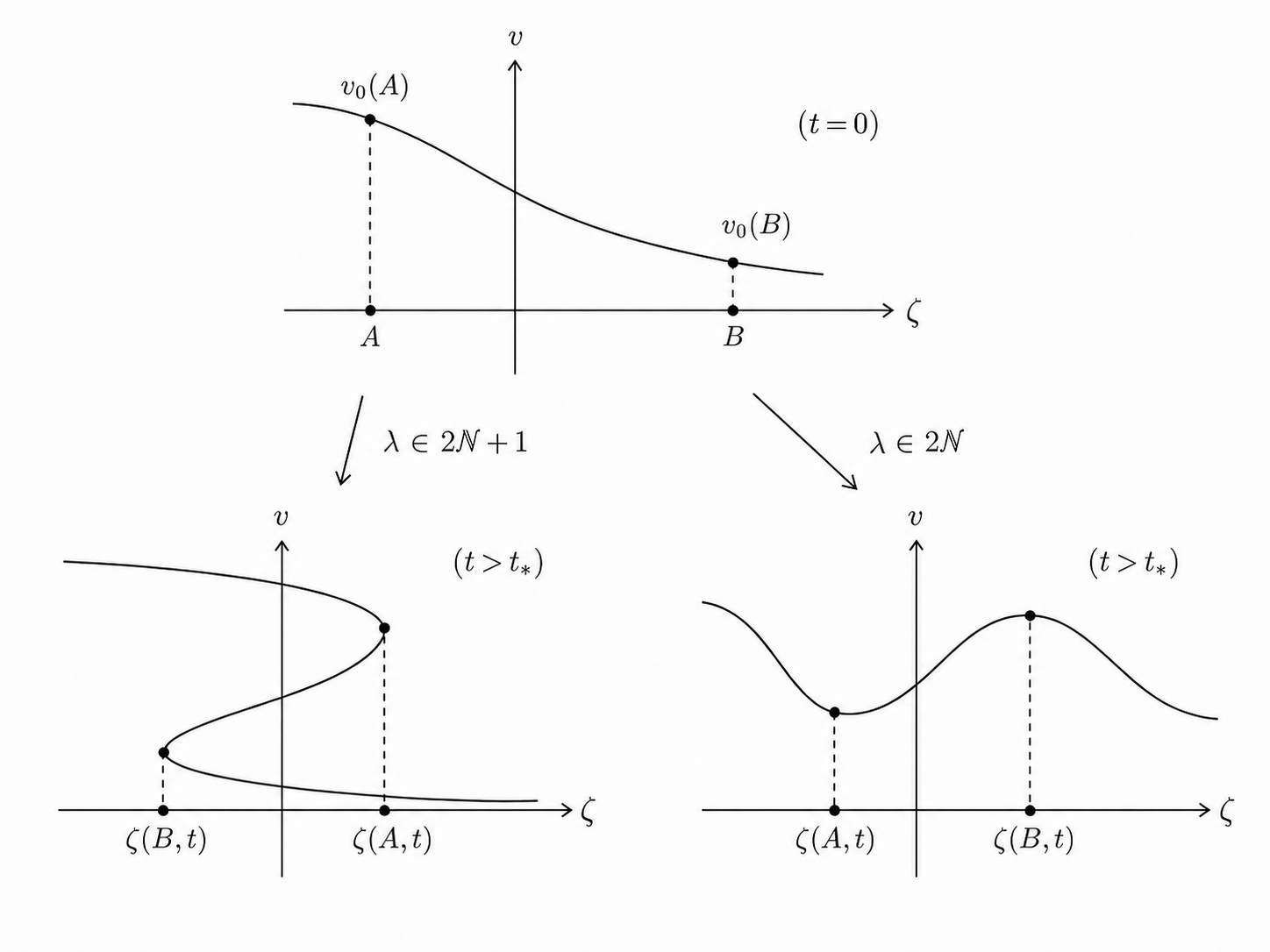
Refer to caption
Figure 2. Schematic post-breaking dynamics for even and odd values of λ\displaystyle\lambda.

For this reason, throughout the paper we restrict attention to λ∈2​ℕ\displaystyle\lambda\in 2\mathbb{N}.

We first describe the local geometry of the Lagrangian singular set 𝒮L\displaystyle\mathcal{S}_{L} near the first breaking point.

Lemma 3.4 (Local structure of the Lagrangian singular set).

Near a=a0\displaystyle a=a_{0}, the Lagrangian singular set 𝒮L\displaystyle\mathcal{S}_{L} defined in (3.6) is given by the smooth graph

t=ts​(a),ts​(a):=−λv0′​(a).t=t_{s}(a),\qquad t_{s}(a):=-\frac{\lambda}{v_{0}^{\prime}(a)}.

At the first singular point (a0,t∗)\displaystyle(a_{0},t_{*}), ts′​(a0)=0,\displaystyle t_{s}^{\prime}(a_{0})=0, and

(3.12) ts′′​(a0)=λ​v0(3)​(a0)v0′​(a0)2>0.t_{s}^{\prime\prime}(a_{0})=\lambda\frac{v_{0}^{(3)}(a_{0})}{v_{0}^{\prime}(a_{0})^{2}}>0.

Hence ts\displaystyle t_{s} has a nondegenerate local minimum at a=a0\displaystyle a=a_{0}.

Moreover, the Eulerian projection of the singular curve, Xs​(a):=ζ⁡(a,ts​(a)),\displaystyle X_{s}(a):=\zeta(a,t_{s}(a)), is well defined near a=a0\displaystyle a=a_{0}, and Xs′​(a0)=0.\displaystyle X_{s}^{\prime}(a_{0})=0.

Proof.

Since v0′​(a0)<0,\displaystyle v_{0}^{\prime}(a_{0})<0, the function ts​(a)=−λv0′​(a)\displaystyle\textstyle t_{s}(a)=-\frac{\lambda}{v_{0}^{\prime}(a)} is smooth in a neighborhood of a=a0\displaystyle a=a_{0}. By DHS​(a,t)=0\displaystyle D_{\mathrm{HS}}(a,t)=0 if and only if t=ts​(a)\displaystyle t=t_{s}(a), this gives a local graph representation of 𝒮L\displaystyle\mathcal{S}_{L}.

Differentiating ts\displaystyle t_{s}, we obtain

ts′​(a)=λ​v0′′​(a)v0′​(a)2.t_{s}^{\prime}(a)=\lambda\frac{v_{0}^{\prime\prime}(a)}{v_{0}^{\prime}(a)^{2}}.

Since v0′′​(a0)=0,\displaystyle v_{0}^{\prime\prime}(a_{0})=0, it follows that ts′​(a0)=0.\displaystyle t_{s}^{\prime}(a_{0})=0. Differentiating once more gives

ts′′​(a)=λ⁡(v0(3)​(a)v0′​(a)2−2​v0′′​(a)2v0′​(a)3).t_{s}^{\prime\prime}(a)=\lambda\left(\frac{v_{0}^{(3)}(a)}{v_{0}^{\prime}(a)^{2}}-2\frac{v_{0}^{\prime\prime}(a)^{2}}{v_{0}^{\prime}(a)^{3}}\right).

Evaluating at a=a0\displaystyle a=a_{0} and using v0′′​(a0)=0,v0(3)​(a0)>0,\displaystyle v_{0}^{\prime\prime}(a_{0})=0,v_{0}^{(3)}(a_{0})>0, we obtain (3.12). Thus ts\displaystyle t_{s} has a nondegenerate local minimum at a=a0\displaystyle a=a_{0}. In particular, the Lagrangian singular curve has a horizontal tangent at the first breaking point (a0,t∗)\displaystyle(a_{0},t_{*}).

We next consider its Eulerian projection Xs​(a)=ζ⁡(a,ts​(a)).\displaystyle X_{s}(a)=\zeta(a,t_{s}(a)). By the chain rule, Xs′​(a)=ζa​(a,ts​(a))+ζt​(a,ts​(a))​ts′​(a).\displaystyle X_{s}^{\prime}(a)=\zeta_{a}(a,t_{s}(a))+\zeta_{t}(a,t_{s}(a))\,t_{s}^{\prime}(a). At a=a0\displaystyle a=a_{0}, we have ζa​(a0,t∗)=0\displaystyle\zeta_{a}(a_{0},t_{*})=0 by Lemma 3.1, while ts′​(a0)=0.\displaystyle t_{s}^{\prime}(a_{0})=0. Therefore, Xs′​(a0)=0.\displaystyle X_{s}^{\prime}(a_{0})=0. This completes the proof. ∎

The nondegenerate minimum of ts\displaystyle t_{s} immediately yields the bifurcation of the singular label a0\displaystyle a_{0} into two branches a−​(t)\displaystyle a_{-}(t) and a+​(t)\displaystyle a_{+}(t) for t>t∗\displaystyle t>t_{*} sufficiently close to t∗\displaystyle t_{*}.

3.2. Emergence of a pair of cuspons

We now describe the short-time post-breaking geometry and show that a pair of cusps emerges from the first breaking point.

A useful feature of the generalized Hunter–Saxton equation is that its Lagrangian degeneracy is completely explicit. Indeed, by (3.10),

ζa​(a,t)=DHS​(a,t)λ,DHS​(a,t)=1+tλ​v0′​(a).\zeta_{a}(a,t)=D_{\mathrm{HS}}(a,t)^{\lambda},\qquad D_{\mathrm{HS}}(a,t)=1+\frac{t}{\lambda}v_{0}^{\prime}(a).

Thus the singular labels are characterized simply by

(3.13) DHS​(a,t)=0,equivalentlyv0′​(a)=−λt.D_{\mathrm{HS}}(a,t)=0,\qquad\text{equivalently}\qquad v_{0}^{\prime}(a)=-\frac{\lambda}{t}.

This explicit characterization is in contrast with the Camassa–Holm case, where the corresponding singular labels are governed by the nonlocal Lagrangian dynamics.

By (3.5), the first singularity occurs at the label-time pair (a0,t∗)\displaystyle(a_{0},t_{*}), where t∗=−λv0′​(a0).\displaystyle\textstyle t_{*}=-\frac{\lambda}{v_{0}^{\prime}(a_{0})}. Moreover, after decreasing εHS>0\displaystyle\varepsilon_{\mathrm{HS}}>0 if necessary, for every t∈(t∗,t∗+εHS)\displaystyle t\in(t_{*},t_{*}+\varepsilon_{\mathrm{HS}}) the level equation (3.13) has exactly two solutions near a0\displaystyle a_{0}, which we denote by

a−​(t)<a0<a+​(t).a_{-}(t)<a_{0}<a_{+}(t).

Equivalently,

ζa​(a±​(t),t)=0.\zeta_{a}(a_{\pm}(t),t)=0.

The two branches a±​(t)\displaystyle a_{\pm}(t) bifurcate from the first breaking label:

a±​(t)⟶a0as ​t↓t∗.a_{\pm}(t)\longrightarrow a_{0}\qquad\text{as }t\downarrow t_{*}.

Since no confusion with the Camassa–Holm variables will arise, we use the same notation a±​(t)\displaystyle a_{\pm}(t) for the two post-breaking singular labels and define their Eulerian images by

x±​(t):=ζ⁡(a±​(t),t).x_{\pm}(t):=\zeta(a_{\pm}(t),t).

Thus we also use the same notation x±​(t)\displaystyle x_{\pm}(t) as in the Camassa–Holm setting. We shall show below that x−​(t)\displaystyle x_{-}(t) and x+​(t)\displaystyle x_{+}(t) are precisely the locations of the two cusps.

Lemma 3.5 (Reversal of the Lagrangian profile and emergence of a cusp pair).

There exists εHS>0\displaystyle\varepsilon_{\mathrm{HS}}>0 such that the following hold.

For t<t∗\displaystyle t<t_{*}, the Lagrangian profile VHS​(a,t):=v⁡(ζ⁡(a,t),t)\displaystyle V_{\mathrm{HS}}(a,t):=v(\zeta(a,t),t) is strictly decreasing in a neighborhood of a=a0\displaystyle a=a_{0}. In particular, for a,b\displaystyle a,b sufficiently close to a0\displaystyle a_{0} with b<a0<a,\displaystyle b<a_{0}<a, we have

(3.14) v⁡(ζ⁡(b,t),t)>v⁡(ζ⁡(a0,t),t)>v⁡(ζ⁡(a,t),t).v(\zeta(b,t),t)>v(\zeta(a_{0},t),t)>v(\zeta(a,t),t).

By contrast, for every t∈(t∗,t∗+εHS),\displaystyle t\in(t_{*},t_{*}+\varepsilon_{\mathrm{HS}}), the Lagrangian profile is strictly increasing on (a−​(t),a+​(t)).\displaystyle(a_{-}(t),a_{+}(t)). Consequently, for a−​(t)<b<a0<a<a+​(t),\displaystyle a_{-}(t)<b<a_{0}<a<a_{+}(t), we have

(3.15) v⁡(ζ⁡(b,t),t)<v⁡(ζ⁡(a0,t),t)<v⁡(ζ⁡(a,t),t).v(\zeta(b,t),t)<v(\zeta(a_{0},t),t)<v(\zeta(a,t),t).

Moreover,

|vx​(ζ⁡(a,t),t)|⟶∞as ​a→a±​(t).\left|v_{x}(\zeta(a,t),t)\right|\longrightarrow\infty\qquad\text{as }a\to a_{\pm}(t).

Hence the continuous Eulerian profile develops two singular points at x±​(t)=ζ⁡(a±​(t),t),\displaystyle x_{\pm}(t)=\zeta(a_{\pm}(t),t), with unbounded spatial slope.

Proof.

By Lemma 3.1,

(3.16) ∂aVHS​(a,t)=v0′​(a)​DHS​(a,t)λ−1,\partial_{a}V_{\mathrm{HS}}(a,t)=v_{0}^{\prime}(a)D_{\mathrm{HS}}(a,t)^{\lambda-1},

where DHS​(a,t)=1+tλ​v0′​(a).\displaystyle\textstyle D_{\mathrm{HS}}(a,t)=1+\frac{t}{\lambda}v_{0}^{\prime}(a).

For every t<t∗\displaystyle t<t_{*}, the definition of the first singular time gives DHS​(a,t)>0​ for all ​a∈ℝ.\displaystyle D_{\mathrm{HS}}(a,t)>0\text{ for all }a\in\mathbb{R}. Since v0′​(a0)<0,\displaystyle v_{0}^{\prime}(a_{0})<0, continuity of v0′\displaystyle v_{0}^{\prime} yields a neighborhood of a0\displaystyle a_{0} on which v0′<0\displaystyle v_{0}^{\prime}<0. Because λ−1\displaystyle\lambda-1 is odd, it follows from (3.16) that ∂aVHS​(a,t)<0\displaystyle\partial_{a}V_{\mathrm{HS}}(a,t)<0 in this neighborhood. Thus VHS​(⋅,t)\displaystyle V_{\mathrm{HS}}(\cdot,t) is strictly decreasing near a0\displaystyle a_{0}, which proves (3.14).

We now fix t∈(t∗,t∗+εHS).\displaystyle t\in(t_{*},t_{*}+\varepsilon_{\mathrm{HS}}). By the definition of the two post-breaking singular labels, DHS​(a±​(t),t)=0,\displaystyle D_{\mathrm{HS}}(a_{\pm}(t),t)=0, or equivalently, v0′​(a±​(t))=−λt.\displaystyle\textstyle v_{0}^{\prime}(a_{\pm}(t))=-\frac{\lambda}{t}. On the other hand, v0′​(a0)=−λt∗<−λt,\displaystyle\textstyle v_{0}^{\prime}(a_{0})=-\frac{\lambda}{t_{*}}<-\frac{\lambda}{t}, since t>t∗\displaystyle t>t_{*}. Hence DHS​(a0,t)<0.\displaystyle D_{\mathrm{HS}}(a_{0},t)<0. For εHS>0\displaystyle\varepsilon_{\mathrm{HS}}>0 sufficiently small, a−​(t)\displaystyle a_{-}(t) and a+​(t)\displaystyle a_{+}(t) are the only zeros of DHS​(⋅,t)\displaystyle D_{\mathrm{HS}}(\cdot,t) in [a−​(t),a+​(t)]\displaystyle[a_{-}(t),a_{+}(t)]. Therefore, DHS​(a,t)<0​ for ​a∈(a−​(t),a+​(t)).\displaystyle D_{\mathrm{HS}}(a,t)<0\text{ for }a\in(a_{-}(t),a_{+}(t)). In particular, v0′​(a)<−λt<0​ for ​a∈(a−​(t),a+​(t)).\displaystyle\textstyle v_{0}^{\prime}(a)<-\frac{\lambda}{t}<0\text{ for }a\in(a_{-}(t),a_{+}(t)). Since λ−1\displaystyle\lambda-1 is odd, both factors on the right-hand side of (3.16) are negative, and hence

∂aVHS​(a,t)>0for ​a∈(a−​(t),a+​(t)).\partial_{a}V_{\mathrm{HS}}(a,t)>0\qquad\text{for }a\in(a_{-}(t),a_{+}(t)).

Thus VHS​(⋅,t)\displaystyle V_{\mathrm{HS}}(\cdot,t) is strictly increasing on this interval, and (3.15) follows.

Finally, by (3.3),

vx​(ζ⁡(a,t),t)=v0′​(a)DHS​(a,t)v_{x}(\zeta(a,t),t)=\frac{v_{0}^{\prime}(a)}{D_{\mathrm{HS}}(a,t)}

whenever DHS​(a,t)≠0\displaystyle D_{\mathrm{HS}}(a,t)\neq 0. Since DHS​(a±​(t),t)=0,v0′​(a±​(t))=−λt≠0,\displaystyle\textstyle D_{\mathrm{HS}}(a_{\pm}(t),t)=0,v_{0}^{\prime}(a_{\pm}(t))=-\frac{\lambda}{t}\neq 0, we obtain

|vx​(ζ⁡(a,t),t)|⟶∞as ​a→a±​(t).\left|v_{x}(\zeta(a,t),t)\right|\longrightarrow\infty\qquad\text{as }a\to a_{\pm}(t).

Since a↦ζ⁡(a,t)\displaystyle a\mapsto\zeta(a,t) remains strictly increasing and the Eulerian profile reconstructed above is continuous, the points x±​(t)=ζ⁡(a±​(t),t)\displaystyle x_{\pm}(t)=\zeta(a_{\pm}(t),t) are two distinct singular points of the continuous profile with unbounded spatial slope. The precise cusp asymptotics at these points will be established below. ∎

By (3.3) and the uniqueness of the global minimum of v0′\displaystyle v_{0}^{\prime}, the slope becomes singular at the first singular time t=t∗\displaystyle t=t_{*} only at the first breaking point x∗:=ζ⁡(a0,t∗).\displaystyle x_{*}:=\zeta(a_{0},t_{*}). Lemma 3.5 shows that, immediately after t∗\displaystyle t_{*}, the corresponding singular label bifurcates into the two branches a−​(t)\displaystyle a_{-}(t) and a+​(t)\displaystyle a_{+}(t), whose Eulerian images are x±​(t):=ζ⁡(a±​(t),t).\displaystyle x_{\pm}(t):=\zeta(a_{\pm}(t),t). Thus the single singular point x∗\displaystyle x_{*} gives rise to a pair of post-breaking singular points.

The sign structure also determines their orientations. For t∈(t∗,t∗+εHS)\displaystyle t\in(t_{*},t_{*}+\varepsilon_{\mathrm{HS}}), we have

vx​(ζ⁡(a,t),t)>0for ​a∈(a−​(t),a+​(t)),v_{x}(\zeta(a,t),t)>0\qquad\text{for }a\in(a_{-}(t),a_{+}(t)),

whereas vx​(ζ⁡(a,t),t)<0\displaystyle v_{x}(\zeta(a,t),t)<0 immediately outside this interval. Consequently, x−​(t)\displaystyle x_{-}(t) is of local-minimum type and x+​(t)\displaystyle x_{+}(t) is of local-maximum type. This reversal of the local profile is the basic mechanism underlying the formation of the cusp pair: before breaking, the Lagrangian profile is decreasing near a=a0\displaystyle a=a_{0}, while immediately after breaking it becomes increasing between the two singular labels.

We next record that the continued solution remains classical away from the two singular curves.

Lemma 3.6 (Classical regularity away from the cusp pair).

After decreasing εHS>0\displaystyle\varepsilon_{\mathrm{HS}}>0 if necessary, define

ΩHS:={(x,t)∈ℝ×(t∗,t∗+εHS):x≠x−(t),x≠x+(t)}.\Omega_{\mathrm{HS}}:=\left\{(x,t)\in\mathbb{R}\times(t_{*},t_{*}+\varepsilon_{\mathrm{HS}}):x\neq x_{-}(t),\;x\neq x_{+}(t)\right\}.

Then, for every t∈(t∗,t∗+εHS)\displaystyle t\in(t_{*},t_{*}+\varepsilon_{\mathrm{HS}}), it holds that v⁡(⋅,t)∈C1​(ℝ∖{x−​(t),x+​(t)}).\displaystyle v(\cdot,t)\in C^{1}\bigl(\mathbb{R}\setminus\{x_{-}(t),x_{+}(t)\}\bigr). Moreover, vx∈C1​(ΩHS),\displaystyle v_{x}\in C^{1}(\Omega_{\mathrm{HS}}), and v\displaystyle v satisfies the generalized Hunter–Saxton equation (3.1) pointwise on ΩHS\displaystyle\Omega_{\mathrm{HS}}.

Proof.

Let (x,t)∈ΩHS.\displaystyle(x,t)\in\Omega_{\mathrm{HS}}. Since a↦ζ⁡(a,t)\displaystyle a\mapsto\zeta(a,t) is strictly increasing, there exists a unique label a≠a±​(t)\displaystyle a\neq a_{\pm}(t) such that x=ζ⁡(a,t).\displaystyle x=\zeta(a,t). In particular, DHS​(a,t)≠0.\displaystyle D_{\mathrm{HS}}(a,t)\neq 0. By Lemma 3.1, ζa​(a,t)=DHS​(a,t)λ≠0.\displaystyle\zeta_{a}(a,t)=D_{\mathrm{HS}}(a,t)^{\lambda}\neq 0. Hence the map (a,t)⟼(ζ⁡(a,t),t)\displaystyle(a,t)\longmapsto(\zeta(a,t),t) is locally invertible on the preimage of ΩHS\displaystyle\Omega_{\mathrm{HS}}. Since DHS≠0\displaystyle D_{\mathrm{HS}}\neq 0 there, the extended Lagrangian variables ζ\displaystyle\zeta and VHS\displaystyle V_{\mathrm{HS}} are smooth on this region. The inverse function theorem therefore gives a smooth inverse Lagrangian label a=A⁡(x,t)\displaystyle a=A(x,t) on ΩHS\displaystyle\Omega_{\mathrm{HS}}, where A⁡(x,t):=(ζ⁡(⋅,t))−1​(x)\displaystyle A(x,t):=(\zeta(\cdot,t))^{-1}(x).

By the Eulerian reconstruction, v⁡(x,t)=VHS​(A⁡(x,t),t),\displaystyle v(x,t)=V_{\mathrm{HS}}(A(x,t),t), and hence v∈C1​(ΩHS).\displaystyle v\in C^{1}(\Omega_{\mathrm{HS}}). Differentiating with respect to x\displaystyle x and using (3.10)–(3.11), we obtain

(3.17) vx​(x,t)=∂aVHS​(A⁡(x,t),t)∂aζ⁡(A⁡(x,t),t)=v0′​(A⁡(x,t))DHS​(A​(x,t),t).v_{x}(x,t)=\frac{\partial_{a}V_{\mathrm{HS}}(A(x,t),t)}{\partial_{a}\zeta(A(x,t),t)}=\frac{v_{0}^{\prime}(A(x,t))}{D_{\mathrm{HS}}(A(x,t),t)}.

Since DHS≠0\displaystyle D_{\mathrm{HS}}\neq 0 on the region under consideration and A\displaystyle A is smooth, the right-hand side of (3.17) shows that vx∈C1​(ΩHS).\displaystyle v_{x}\in C^{1}(\Omega_{\mathrm{HS}}).

For later use, we also record the second derivative explicitly. Differentiating v0′​(a)DHS​(a,t)\displaystyle\textstyle\frac{v_{0}^{\prime}(a)}{D_{\mathrm{HS}}(a,t)} with respect to a\displaystyle a, and recalling that DHS​(a,t)=1+tλ​v0′​(a),\displaystyle\textstyle D_{\mathrm{HS}}(a,t)=1+\frac{t}{\lambda}v_{0}^{\prime}(a), gives ∂a(v0′​(a)DHS​(a,t))=v0′′​(a)DHS​(a,t)2.\displaystyle\textstyle\partial_{a}\left(\frac{v_{0}^{\prime}(a)}{D_{\mathrm{HS}}(a,t)}\right)=\frac{v_{0}^{\prime\prime}(a)}{D_{\mathrm{HS}}(a,t)^{2}}. Since ζa​(a,t)=DHS​(a,t)λ,\displaystyle\zeta_{a}(a,t)=D_{\mathrm{HS}}(a,t)^{\lambda}, we therefore obtain

vx​x​(ζ⁡(a,t),t)=v0′′​(a)DHS​(a,t)λ+2,v_{xx}(\zeta(a,t),t)=\frac{v_{0}^{\prime\prime}(a)}{D_{\mathrm{HS}}(a,t)^{\lambda+2}},

whenever a≠a±​(t)\displaystyle a\neq a_{\pm}(t). Thus vx​x\displaystyle v_{xx} is continuous on ΩHS\displaystyle\Omega_{\mathrm{HS}}.

It remains to verify the equation. By (3.7)–(3.8),

∂tζ⁡(a,t)=VHS​(a,t)=v⁡(ζ⁡(a,t),t),\partial_{t}\zeta(a,t)=V_{\mathrm{HS}}(a,t)=v(\zeta(a,t),t),

so the extended Lagrangian map continues to satisfy the characteristic equation. Moreover, (3.17) gives vx​(ζ⁡(a,t),t)=v0′​(a)DHS​(a,t).\displaystyle\textstyle v_{x}(\zeta(a,t),t)=\frac{v_{0}^{\prime}(a)}{D_{\mathrm{HS}}(a,t)}. Differentiating with respect to t\displaystyle t at fixed a\displaystyle a, we find

dd​t​vx​(ζ⁡(a,t),t)\displaystyle\frac{d}{dt}v_{x}(\zeta(a,t),t) =−1λ​v0′​(a)2DHS​(a,t)2=−1λ​vx​(ζ⁡(a,t),t)2.\displaystyle=-\frac{1}{\lambda}\frac{v_{0}^{\prime}(a)^{2}}{D_{\mathrm{HS}}(a,t)^{2}}=-\frac{1}{\lambda}v_{x}(\zeta(a,t),t)^{2}.

On the other hand, since ∂tζ⁡(a,t)=v⁡(ζ⁡(a,t),t),\displaystyle\partial_{t}\zeta(a,t)=v(\zeta(a,t),t), the chain rule yields

dd​t​vx​(ζ⁡(a,t),t)=vt​x​(ζ⁡(a,t),t)+v⁡(ζ⁡(a,t),t)​vx​x​(ζ⁡(a,t),t).\frac{d}{dt}v_{x}(\zeta(a,t),t)=v_{tx}(\zeta(a,t),t)+v(\zeta(a,t),t)v_{xx}(\zeta(a,t),t).

Combining the last two identities, we obtain

vt​x+v​vx​x=−1λ​vx2v_{tx}+vv_{xx}=-\frac{1}{\lambda}v_{x}^{2}

at every point of ΩHS\displaystyle\Omega_{\mathrm{HS}}. Hence v\displaystyle v is a classical solution of the generalized Hunter–Saxton equation (3.1) on ΩHS\displaystyle\Omega_{\mathrm{HS}}. ∎

3.3. Sharp regularity and dynamics of the cuspon pair

We first determine the sharp spatial regularity at the first breaking point and at the two post-breaking cusp locations.

Lemma 3.7 (Sharp regularity of the cusp pair).

There exists εHS>0\displaystyle\varepsilon_{\mathrm{HS}}>0 such that the following hold.

At the first singular time t=t∗\displaystyle t=t_{*}, the pointwise Hölder exponent of v⁡(⋅,t∗)\displaystyle v(\cdot,t_{*}) at x∗=ζ⁡(a0,t∗)\displaystyle x_{*}=\zeta(a_{0},t_{*}) is exactly

α∗:=2​λ−12​λ+1.\alpha_{*}:=\frac{2\lambda-1}{2\lambda+1}.

More precisely,

(3.18) 0<limx→x∗|v⁡(x,t∗)−v⁡(x∗,t∗)||x−x∗|α∗<∞.0<\lim_{x\to x_{*}}\frac{|v(x,t_{*})-v(x_{*},t_{*})|}{|x-x_{*}|^{\alpha_{*}}}<\infty.

For every t∈(t∗,t∗+εHS),\displaystyle t\in(t_{*},t_{*}+\varepsilon_{\mathrm{HS}}), the pointwise Hölder exponent of v⁡(⋅,t)\displaystyle v(\cdot,t) at each of the two post-breaking singular points x±​(t)=ζ⁡(a±​(t),t)\displaystyle x_{\pm}(t)=\zeta(a_{\pm}(t),t) is exactly

αcusp:=λλ+1.\alpha_{\mathrm{cusp}}:=\frac{\lambda}{\lambda+1}.

More precisely, for either choice of sign,

(3.19) 0<limx→x±​(t)|v⁡(x,t)−v⁡(x±​(t),t)||x−x±​(t)|αcusp<∞.0<\lim_{x\to x_{\pm}(t)}\frac{|v(x,t)-v(x_{\pm}(t),t)|}{|x-x_{\pm}(t)|^{\alpha_{\mathrm{cusp}}}}<\infty.

In particular, both exponents are sharp.

Proof.

We treat the first breaking point and the post-breaking cusp points simultaneously.

Fix t∈[t∗,t∗+εHS)\displaystyle t\in[t_{*},t_{*}+\varepsilon_{\mathrm{HS}}), and let as\displaystyle a_{s} denote one of the singular labels under consideration:

as:={a0,t=t∗,a−​(t)​or​a+​(t),t>t∗.a_{s}:=\begin{cases}a_{0},&t=t_{*},\\[2.84526pt] a_{-}(t)\ \text{or}\ a_{+}(t),&t>t_{*}.\end{cases}

Set xs:=ζ⁡(as,t).\displaystyle x_{s}:=\zeta(a_{s},t). We also define

m:={2,t=t∗,1,t>t∗.m:=\begin{cases}2,&t=t_{*},\\[2.84526pt] 1,&t>t_{*}.\end{cases}

By the definition of a singular label,

(3.20) DHS​(as,t)=0,v0′​(as)=−λt.D_{\mathrm{HS}}(a_{s},t)=0,\qquad v_{0}^{\prime}(a_{s})=-\frac{\lambda}{t}.

At t=t∗\displaystyle t=t_{*}, the nondegeneracy of the minimum of v0′\displaystyle v_{0}^{\prime} gives v0′′​(a0)=0,v0(3)​(a0)≠0,\displaystyle v_{0}^{\prime\prime}(a_{0})=0,v_{0}^{(3)}(a_{0})\neq 0, whereas for t>t∗\displaystyle t>t_{*} sufficiently close to t∗\displaystyle t_{*}, the two level crossings a±​(t)\displaystyle a_{\pm}(t) are simple, so that v0′′​(a±​(t))≠0.\displaystyle v_{0}^{\prime\prime}(a_{\pm}(t))\neq 0. Consequently, as α→as\displaystyle\alpha\to a_{s},

(3.21) DHS​(α,t)=ds​(t)​(α−as)m+O⁡(|α−as|m+1),D_{\mathrm{HS}}(\alpha,t)=d_{s}(t)(\alpha-a_{s})^{m}+O\left(|\alpha-a_{s}|^{m+1}\right),

where

ds​(t):=tλ​v0(m+1)​(as)m!≠0.d_{s}(t):=\frac{t}{\lambda}\frac{v_{0}^{(m+1)}(a_{s})}{m!}\neq 0.

By (3.10), ζa​(a,t)=DHS​(a,t)λ.\displaystyle\zeta_{a}(a,t)=D_{\mathrm{HS}}(a,t)^{\lambda}. Hence, using (3.21),

ζ⁡(a,t)−ζ⁡(as,t)\displaystyle\displaystyle\zeta(a,t)-\zeta(a_{s},t) =∫asaDHS​(α,t)λ​𝑑α=ds​(t)λm​λ+1​(a−as)m​λ+1+O⁡(|a−as|m​λ+2).\displaystyle\displaystyle=\int_{a_{s}}^{a}D_{\mathrm{HS}}(\alpha,t)^{\lambda}\,d\alpha=\frac{d_{s}(t)^{\lambda}}{m\lambda+1}(a-a_{s})^{m\lambda+1}+O\left(|a-a_{s}|^{m\lambda+2}\right).

Setting Cs​(t):=ds​(t)λm​λ+1,\displaystyle\textstyle C_{s}(t):=\frac{d_{s}(t)^{\lambda}}{m\lambda+1}, we obtain

(3.22) ζ⁡(a,t)−xs=Cs​(t)​(a−as)m​λ+1+O⁡(|a−as|m​λ+2),\zeta(a,t)-x_{s}=C_{s}(t)(a-a_{s})^{m\lambda+1}+O\left(|a-a_{s}|^{m\lambda+2}\right),

where Cs​(t)≠0\displaystyle C_{s}(t)\neq 0.

We next expand the Lagrangian profile. By (3.11), we see that ∂aVHS​(a,t)=v0′​(a)​DHS​(a,t)λ−1.\displaystyle\partial_{a}V_{\mathrm{HS}}(a,t)=v_{0}^{\prime}(a)D_{\mathrm{HS}}(a,t)^{\lambda-1}. Using (3.20) and (3.21), we obtain

VHS​(a,t)−VHS​(as,t)\displaystyle\displaystyle V_{\mathrm{HS}}(a,t)-V_{\mathrm{HS}}(a_{s},t) =∫asav0′​(α)​DHS​(α,t)λ−1​𝑑α\displaystyle\displaystyle=\int_{a_{s}}^{a}v_{0}^{\prime}(\alpha)D_{\mathrm{HS}}(\alpha,t)^{\lambda-1}\,d\alpha
=−λt​ds​(t)λ−1m⁡(λ−1)+1​(a−as)m⁡(λ−1)+1+O⁡(|a−as|m⁡(λ−1)+2).\displaystyle\displaystyle=-\frac{\lambda}{t}\frac{d_{s}(t)^{\lambda-1}}{m(\lambda-1)+1}(a-a_{s})^{m(\lambda-1)+1}+O\left(|a-a_{s}|^{m(\lambda-1)+2}\right).

Let C~s​(t):=−λt​ds​(t)λ−1m⁡(λ−1)+1.\displaystyle\textstyle\widetilde{C}_{s}(t):=-\frac{\lambda}{t}\frac{d_{s}(t)^{\lambda-1}}{m(\lambda-1)+1}. Then C~s​(t)≠0\displaystyle\widetilde{C}_{s}(t)\neq 0, and

(3.23) VHS​(a,t)−VHS​(as,t)=C~s​(t)​(a−as)m⁡(λ−1)+1+O⁡(|a−as|m⁡(λ−1)+2).V_{\mathrm{HS}}(a,t)-V_{\mathrm{HS}}(a_{s},t)=\widetilde{C}_{s}(t)(a-a_{s})^{m(\lambda-1)+1}+O\left(|a-a_{s}|^{m(\lambda-1)+2}\right).

Combining (3.22) and (3.23), we find that the critical Hölder exponent at xs\displaystyle x_{s} is

αs=m⁡(λ−1)+1m​λ+1.\alpha_{s}=\frac{m(\lambda-1)+1}{m\lambda+1}.

Indeed,

(3.24) |VHS​(a,t)−VHS​(as,t)||ζ⁡(a,t)−ζ⁡(as,t)|αs⟶|C~s​(t)||Cs​(t)|αs∈(0,∞)\frac{|V_{\mathrm{HS}}(a,t)-V_{\mathrm{HS}}(a_{s},t)|}{|\zeta(a,t)-\zeta(a_{s},t)|^{\alpha_{s}}}\longrightarrow\frac{|\widetilde{C}_{s}(t)|}{|C_{s}(t)|^{\alpha_{s}}}\in(0,\infty)

as a→as\displaystyle a\to a_{s}.

At the first singular time t=t∗\displaystyle t=t_{*}, we have m=2\displaystyle m=2, and therefore

αs=2​(λ−1)+12​λ+1=2​λ−12​λ+1.\alpha_{s}=\frac{2(\lambda-1)+1}{2\lambda+1}=\frac{2\lambda-1}{2\lambda+1}.

This proves (3.18).

For every t>t∗\displaystyle t>t_{*} sufficiently close to t∗\displaystyle t_{*}, each singular label a±​(t)\displaystyle a_{\pm}(t) is a simple zero of DHS​(⋅,t)\displaystyle D_{\mathrm{HS}}(\cdot,t), so that m=1\displaystyle m=1. Hence

αs=λλ+1,\alpha_{s}=\frac{\lambda}{\lambda+1},

which proves (3.19) at both x−​(t)\displaystyle x_{-}(t) and x+​(t)\displaystyle x_{+}(t).

The positivity and finiteness of the limit in (3.24) also show that these exponents cannot be improved. Thus the stated Hölder exponents are sharp. ∎

Remark 3.8 (Improved regularity after cusp bifurcation).

An interesting feature of the post-breaking dynamics is that the two cuspons are more regular than the profile at the first breaking point. Indeed, λλ+1>2​λ−12​λ+1.\displaystyle\textstyle\frac{\lambda}{\lambda+1}>\frac{2\lambda-1}{2\lambda+1}. Thus, at t=t∗\displaystyle t=t_{*}, the first singular profile has the sharp pointwise Hölder exponent 2​λ−12​λ+1,\displaystyle\textstyle\frac{2\lambda-1}{2\lambda+1}, whereas immediately after breaking each of the two cuspons has the strictly larger exponent λλ+1.\displaystyle\textstyle\frac{\lambda}{\lambda+1}. In this sense, the bifurcation of the single breaking singularity into an anticuspon–cuspon pair is accompanied by an improvement of the pointwise spatial regularity at the singular points.

Lemma 3.9 (Outward motion of the cusp pair).

After decreasing εHS>0\displaystyle\varepsilon_{\mathrm{HS}}>0 if necessary, let t∈(t∗,t∗+εHS).\displaystyle t\in(t_{*},t_{*}+\varepsilon_{\mathrm{HS}}). Then the two cusp locations x±​(t):=ζ⁡(a±​(t),t)\displaystyle x_{\pm}(t):=\zeta(a_{\pm}(t),t) move away from the central trajectory x0​(t):=ζ⁡(a0,t).\displaystyle x_{0}(t):=\zeta(a_{0},t). More precisely,

dd​t​(x+​(t)−x0​(t))>0,dd​t​(x0​(t)−x−​(t))>0.\frac{d}{dt}\bigl(x_{+}(t)-x_{0}(t)\bigr)>0,\qquad\frac{d}{dt}\bigl(x_{0}(t)-x_{-}(t)\bigr)>0.

Consequently,

dd​t​(x+​(t)−x−​(t))>0.\frac{d}{dt}\bigl(x_{+}(t)-x_{-}(t)\bigr)>0.

In fact,

x−′​(t)<x0′​(t)<x+′​(t).x_{-}^{\prime}(t)<x_{0}^{\prime}(t)<x_{+}^{\prime}(t).
Proof.

Since a±​(t)\displaystyle a_{\pm}(t) are simple zeros of DHS​(⋅,t)\displaystyle D_{\mathrm{HS}}(\cdot,t), they depend smoothly on t\displaystyle t for t>t∗\displaystyle t>t_{*} sufficiently close to t∗\displaystyle t_{*}. Moreover, ζa​(a±​(t),t)=0.\displaystyle\zeta_{a}(a_{\pm}(t),t)=0. By (3.9),

dd​t​x±​(t)\displaystyle\frac{d}{dt}x_{\pm}(t) =ζt​(a±​(t),t)+ζa​(a±​(t),t)​a±′​(t)=VHS​(a±​(t),t).\displaystyle=\zeta_{t}(a_{\pm}(t),t)+\zeta_{a}(a_{\pm}(t),t)a_{\pm}^{\prime}(t)=V_{\mathrm{HS}}(a_{\pm}(t),t).

Since a0\displaystyle a_{0} is fixed,

x0′​(t)=ζt​(a0,t)=VHS​(a0,t).x_{0}^{\prime}(t)=\zeta_{t}(a_{0},t)=V_{\mathrm{HS}}(a_{0},t).

Hence

dd​t​(x+​(t)−x0​(t))=VHS​(a+​(t),t)−VHS​(a0,t).\frac{d}{dt}\bigl(x_{+}(t)-x_{0}(t)\bigr)=V_{\mathrm{HS}}(a_{+}(t),t)-V_{\mathrm{HS}}(a_{0},t).

By the sign property established in the proof of Lemma 3.5,

∂aVHS​(a,t)>0for ​a∈(a−​(t),a+​(t)).\partial_{a}V_{\mathrm{HS}}(a,t)>0\qquad\text{for }a\in(a_{-}(t),a_{+}(t)).

Thus

VHS​(a+​(t),t)−VHS​(a0,t)=∫a0a+​(t)∂aVHS​(a,t)​𝑑a>0,V_{\mathrm{HS}}(a_{+}(t),t)-V_{\mathrm{HS}}(a_{0},t)=\int_{a_{0}}^{a_{+}(t)}\partial_{a}V_{\mathrm{HS}}(a,t)\,da>0,

and therefore

dd​t​(x+​(t)−x0​(t))>0.\frac{d}{dt}\bigl(x_{+}(t)-x_{0}(t)\bigr)>0.

Similarly,

dd​t​(x0​(t)−x−​(t))=VHS​(a0,t)−VHS​(a−​(t),t)\frac{d}{dt}\bigl(x_{0}(t)-x_{-}(t)\bigr)=V_{\mathrm{HS}}(a_{0},t)-V_{\mathrm{HS}}(a_{-}(t),t)

and hence

VHS​(a0,t)−VHS​(a−​(t),t)=∫a−​(t)a0∂aVHS​(a,t)​𝑑a>0.V_{\mathrm{HS}}(a_{0},t)-V_{\mathrm{HS}}(a_{-}(t),t)=\int_{a_{-}(t)}^{a_{0}}\partial_{a}V_{\mathrm{HS}}(a,t)\,da>0.

Therefore,

dd​t​(x0​(t)−x−​(t))>0.\frac{d}{dt}\bigl(x_{0}(t)-x_{-}(t)\bigr)>0.

Finally, x+​(t)−x−​(t)=(x+​(t)−x0​(t))+(x0​(t)−x−​(t)),\displaystyle x_{+}(t)-x_{-}(t)=\bigl(x_{+}(t)-x_{0}(t)\bigr)+\bigl(x_{0}(t)-x_{-}(t)\bigr), so

dd​t​(x+​(t)−x−​(t))>0.\frac{d}{dt}\bigl(x_{+}(t)-x_{-}(t)\bigr)>0.

This completes the proof. ∎

3.4. Completion of the proof of Theorem 1.4

Proof of (1.5) and (1.6) in Theorem 1.4.

Since λ\displaystyle\lambda is even, Lemma 3.1 gives ζa​(a,t)=DHS​(a,t)λ≥0.\displaystyle\zeta_{a}(a,t)=D_{\mathrm{HS}}(a,t)^{\lambda}\geq 0. Moreover, for t∈[0,t∗+εHS),\displaystyle t\in[0,t_{*}+\varepsilon_{\mathrm{HS}}), the function DHS​(⋅,t)\displaystyle D_{\mathrm{HS}}(\cdot,t) does not vanish identically on any nontrivial interval. Hence, for any a1<a2\displaystyle a_{1}<a_{2},

ζ⁡(a2,t)−ζ⁡(a1,t)=∫a1a2DHS​(a,t)λ​𝑑a>0.\zeta(a_{2},t)-\zeta(a_{1},t)=\int_{a_{1}}^{a_{2}}D_{\mathrm{HS}}(a,t)^{\lambda}\,da>0.

Thus a↦ζ⁡(a,t)\displaystyle a\mapsto\zeta(a,t) is strictly increasing and admits a continuous inverse on its image. Consequently, the Eulerian profile v⁡(x,t)=VHS​(ζ−1​(x,t),t)\displaystyle v(x,t)=V_{\mathrm{HS}}\bigl(\zeta^{-1}(x,t),t\bigr) is well defined and continuous for t∈[0,t∗+εHS)\displaystyle t\in[0,t_{*}+\varepsilon_{\mathrm{HS}}).

We next prove conservation of the Lλ\displaystyle L^{\lambda}-norm of the slope. By (3.10) and (3.11),

ζa​(a,t)=DHS​(a,t)λ,∂aVHS​(a,t)=v0′​(a)​DHS​(a,t)λ−1.\zeta_{a}(a,t)=D_{\mathrm{HS}}(a,t)^{\lambda},\qquad\partial_{a}V_{\mathrm{HS}}(a,t)=v_{0}^{\prime}(a)D_{\mathrm{HS}}(a,t)^{\lambda-1}.

Away from the singular labels,

vx​(ζ⁡(a,t),t)=∂aVHS​(a,t)ζa​(a,t)=v0′​(a)DHS​(a,t).v_{x}(\zeta(a,t),t)=\frac{\partial_{a}V_{\mathrm{HS}}(a,t)}{\zeta_{a}(a,t)}=\frac{v_{0}^{\prime}(a)}{D_{\mathrm{HS}}(a,t)}.

Therefore, using the change of variables x=ζ⁡(a,t)\displaystyle x=\zeta(a,t),

∫ℝ|vx​(x,t)|λ​𝑑x\displaystyle\int_{\mathbb{R}}|v_{x}(x,t)|^{\lambda}\,dx =∫ℝ|∂aVHS​(a,t)ζa​(a,t)|λ​ζa​(a,t)​da=∫ℝ|∂aVHS​(a,t)|λζa​(a,t)λ−1​da=∫ℝ|v0′​(a)|λ​da.\displaystyle=\int_{\mathbb{R}}\left|\frac{\partial_{a}V_{\mathrm{HS}}(a,t)}{\zeta_{a}(a,t)}\right|^{\lambda}\zeta_{a}(a,t)\,da=\int_{\mathbb{R}}\frac{|\partial_{a}V_{\mathrm{HS}}(a,t)|^{\lambda}}{\zeta_{a}(a,t)^{\lambda-1}}\,da=\int_{\mathbb{R}}|v_{0}^{\prime}(a)|^{\lambda}\,da.

Hence ‖vx​(⋅,t)‖Lλ​(ℝ)=‖v0′‖Lλ​(ℝ)\displaystyle\|v_{x}(\cdot,t)\|_{L^{\lambda}(\mathbb{R})}=\|v_{0}^{\prime}\|_{L^{\lambda}(\mathbb{R})} for every t∈[0,t∗+εHS)\displaystyle t\in[0,t_{*}+\varepsilon_{\mathrm{HS}}).

We also obtain an L1\displaystyle L^{1}-bound for the slope. By (3.11),

|∂aVHS​(a,t)|=|v0′​(a)|​|1+tλ​v0′​(a)|λ−1.|\partial_{a}V_{\mathrm{HS}}(a,t)|=|v_{0}^{\prime}(a)|\left|1+\frac{t}{\lambda}v_{0}^{\prime}(a)\right|^{\lambda-1}.

Using |1+z|λ−1≤2λ−1​(1+|z|λ−1),\displaystyle|1+z|^{\lambda-1}\leq 2^{\lambda-1}\bigl(1+|z|^{\lambda-1}\bigr), we obtain

|∂aVHS​(a,t)|≤2λ−1​(|v0′​(a)|+(tλ)λ−1​|v0′​(a)|λ).|\partial_{a}V_{\mathrm{HS}}(a,t)|\leq 2^{\lambda-1}\left(|v_{0}^{\prime}(a)|+\left(\frac{t}{\lambda}\right)^{\lambda-1}|v_{0}^{\prime}(a)|^{\lambda}\right).

Since v0′∈L1​(ℝ)∩Lλ​(ℝ),\displaystyle v_{0}^{\prime}\in L^{1}(\mathbb{R})\cap L^{\lambda}(\mathbb{R}), it follows that ∂aVHS​(⋅,t)∈L1​(ℝ).\displaystyle\partial_{a}V_{\mathrm{HS}}(\cdot,t)\in L^{1}(\mathbb{R}). Again using the monotone change of variables,

∫ℝ|vx​(x,t)|​𝑑x\displaystyle\int_{\mathbb{R}}|v_{x}(x,t)|\,dx =∫ℝ|∂aVHS​(a,t)ζa​(a,t)|​ζa​(a,t)​da=∫ℝ|∂aVHS​(a,t)|​da<∞.\displaystyle=\int_{\mathbb{R}}\left|\frac{\partial_{a}V_{\mathrm{HS}}(a,t)}{\zeta_{a}(a,t)}\right|\zeta_{a}(a,t)\,da=\int_{\mathbb{R}}|\partial_{a}V_{\mathrm{HS}}(a,t)|\,da<\infty.

Thus vx​(⋅,t)∈L1​(ℝ).\displaystyle v_{x}(\cdot,t)\in L^{1}(\mathbb{R}).

Finally, we prove the local boundedness of v\displaystyle v. For any a,b∈ℝ\displaystyle a,b\in\mathbb{R},

VHS​(a,t)−VHS​(b,t)=∫ba∂αVHS​(α,t)​𝑑α.V_{\mathrm{HS}}(a,t)-V_{\mathrm{HS}}(b,t)=\int_{b}^{a}\partial_{\alpha}V_{\mathrm{HS}}(\alpha,t)\,d\alpha.

Therefore,

|VHS​(a,t)|≤|VHS​(a0,t)|+‖∂aVHS​(⋅,t)‖L1​(ℝ).|V_{\mathrm{HS}}(a,t)|\leq|V_{\mathrm{HS}}(a_{0},t)|+\|\partial_{a}V_{\mathrm{HS}}(\cdot,t)\|_{L^{1}(\mathbb{R})}.

By the construction of the extended Lagrangian flow, VHS​(a0,t)=ζt​(a0,t)\displaystyle V_{\mathrm{HS}}(a_{0},t)=\zeta_{t}(a_{0},t) is continuous in t\displaystyle t. Hence it remains bounded on every compact time interval. Moreover, the preceding L1\displaystyle L^{1}-estimate is uniform for t\displaystyle t in compact subsets of [0,t∗+εHS)\displaystyle[0,t_{*}+\varepsilon_{\mathrm{HS}}). Consequently, v∈Lloc∞(ℝ×[0,t∗+εHS)).\displaystyle v\in L^{\infty}_{\mathrm{loc}}\bigl(\mathbb{R}\times[0,t_{*}+\varepsilon_{\mathrm{HS}})\bigr). This proves (1.5) and (1.6). ∎

The next lemma verifies that the Eulerian profile constructed above indeed satisfies the generalized Hunter–Saxton equation in the weak sense.

Lemma 3.10 (Verification of the Eulerian weak formulation).

The function v⁡(x,t)=VHS​(ζ−1​(x,t),t)\displaystyle v(x,t)=V_{\mathrm{HS}}\bigl(\zeta^{-1}(x,t),t\bigr) is an Eulerian weak solution of (1.4) on [0,t∗+εHS)\displaystyle[0,t_{*}+\varepsilon_{\mathrm{HS}}). More precisely, for every ψ∈Cc1(ℝ×[0,t∗+εHS)),\displaystyle\psi\in C_{c}^{1}\bigl(\mathbb{R}\times[0,t_{*}+\varepsilon_{\mathrm{HS}})\bigr), we have

∫0t∗+εHS∫ℝ[vx​ψt+v​vx​ψx+(1−1λ)​vx2​ψ]​dx​dt+∫ℝv0′​(x)​ψ​(x,0)​dx=0.\displaystyle\int_{0}^{t_{*}+\varepsilon_{\mathrm{HS}}}\int_{\mathbb{R}}\left[v_{x}\psi_{t}+vv_{x}\psi_{x}+\left(1-\frac{1}{\lambda}\right)v_{x}^{2}\psi\right]\,dx\,dt+\int_{\mathbb{R}}v_{0}^{\prime}(x)\psi(x,0)\,dx=0.
Proof.

Set SHS​(a,t):=vx​(ζ⁡(a,t),t)\displaystyle S_{\mathrm{HS}}(a,t):=v_{x}(\zeta(a,t),t) whenever DHS​(a,t)≠0\displaystyle D_{\mathrm{HS}}(a,t)\neq 0, and let JHS​(a,t):=ζa​(a,t).\displaystyle J_{\mathrm{HS}}(a,t):=\zeta_{a}(a,t). By (3.3) and (3.10),

SHS=v0′DHS,JHS=DHSλS_{\mathrm{HS}}=\frac{v_{0}^{\prime}}{D_{\mathrm{HS}}},\qquad J_{\mathrm{HS}}=D_{\mathrm{HS}}^{\lambda}

on the regular set.

Introduce NHS:=SHS​JHS\displaystyle N_{\mathrm{HS}}:=S_{\mathrm{HS}}J_{\mathrm{HS}} and MHS:=SHS2​JHS.\displaystyle M_{\mathrm{HS}}:=S_{\mathrm{HS}}^{2}J_{\mathrm{HS}}. Using the explicit formulas above, we obtain

NHS(a,t)=v0′(a)DHS(a,t)λ−1 and MHS(a,t)=v0′(a)2DHS(a,t)λ−2.N_{\mathrm{HS}}(a,t)=v_{0}^{\prime}(a)D_{\mathrm{HS}}(a,t)^{\lambda-1}\text{ and }M_{\mathrm{HS}}(a,t)=v_{0}^{\prime}(a)^{2}D_{\mathrm{HS}}(a,t)^{\lambda-2}.

Since λ∈2​ℕ\displaystyle\lambda\in 2\mathbb{N}, both expressions extend continuously through the zero set of DHS\displaystyle D_{\mathrm{HS}}. In particular, they are locally integrable on ℝ×[0,t∗+εHS).\displaystyle\mathbb{R}\times[0,t_{*}+\varepsilon_{\mathrm{HS}}).

Moreover, since

∂tDHS​(a,t)=1λ​v0′​(a),\partial_{t}D_{\mathrm{HS}}(a,t)=\frac{1}{\lambda}v_{0}^{\prime}(a),

we have

(3.25) ∂tNHS=(1−1λ)​MHS\partial_{t}N_{\mathrm{HS}}=\left(1-\frac{1}{\lambda}\right)M_{\mathrm{HS}}

holds across the singular set as well.

Let Ψ⁡(a,t):=ψ⁡(ζ⁡(a,t),t).\displaystyle\Psi(a,t):=\psi(\zeta(a,t),t). Since ζt​(a,t)=VHS​(a,t)=v⁡(ζ⁡(a,t),t),\displaystyle\zeta_{t}(a,t)=V_{\mathrm{HS}}(a,t)=v(\zeta(a,t),t), we have

∂tΨ⁡(a,t)=ψt​(ζ⁡(a,t),t)+v⁡(ζ⁡(a,t),t)​ψx​(ζ⁡(a,t),t).\partial_{t}\Psi(a,t)=\psi_{t}(\zeta(a,t),t)+v(\zeta(a,t),t)\psi_{x}(\zeta(a,t),t).

Since a↦ζ⁡(a,t)\displaystyle a\mapsto\zeta(a,t) is strictly increasing, the change of variables x=ζ⁡(a,t)\displaystyle x=\zeta(a,t) gives

∫0t∗+εHS∫ℝ[vx​ψt+v​vx​ψx+(1−1λ)​vx2​ψ]​𝑑x​𝑑t\displaystyle\int_{0}^{t_{*}+\varepsilon_{\mathrm{HS}}}\int_{\mathbb{R}}\left[v_{x}\psi_{t}+vv_{x}\psi_{x}+\left(1-\frac{1}{\lambda}\right)v_{x}^{2}\psi\right]\,dx\,dt
=∫0t∗+εHS∫ℝ[NHS​(a,t)​∂tΨ⁡(a,t)+(1−1λ)​MHS​(a,t)​Ψ​(a,t)]​da​dt.\displaystyle=\int_{0}^{t_{*}+\varepsilon_{\mathrm{HS}}}\int_{\mathbb{R}}\left[N_{\mathrm{HS}}(a,t)\,\partial_{t}\Psi(a,t)+\left(1-\frac{1}{\lambda}\right)M_{\mathrm{HS}}(a,t)\Psi(a,t)\right]\,da\,dt.

By (3.25), the integrand on the right-hand side is ∂t(NHS​(a,t)​Ψ​(a,t)).\displaystyle\partial_{t}\bigl(N_{\mathrm{HS}}(a,t)\Psi(a,t)\bigr). Hence

∫0t∗+εHS∫ℝ[vxψt+vvxψx+(1−1λ)vx2ψ]dxdt=−∫ℝNHS(a,0)Ψ(a,0)da,\displaystyle\int_{0}^{t_{*}+\varepsilon_{\mathrm{HS}}}\int_{\mathbb{R}}\left[v_{x}\psi_{t}+vv_{x}\psi_{x}+\left(1-\frac{1}{\lambda}\right)v_{x}^{2}\psi\right]\,dx\,dt=-\int_{\mathbb{R}}N_{\mathrm{HS}}(a,0)\Psi(a,0)\,da,

because ψ\displaystyle\psi is compactly supported in ℝ×[0,t∗+εHS)\displaystyle\mathbb{R}\times[0,t_{*}+\varepsilon_{\mathrm{HS}}).

At t=0\displaystyle t=0, DHS​(a,0)=1,ζ⁡(a,0)=a,\displaystyle D_{\mathrm{HS}}(a,0)=1,\zeta(a,0)=a, and therefore NHS​(a,0)=v0′​(a),Ψ⁡(a,0)=ψ⁡(a,0).\displaystyle N_{\mathrm{HS}}(a,0)=v_{0}^{\prime}(a),\Psi(a,0)=\psi(a,0). Thus

∫0t∗+εHS∫ℝ[vx​ψt+v​vx​ψx+(1−1λ)​vx2​ψ]​dx​dt+∫ℝv0′​(x)​ψ​(x,0)​dx=0.\displaystyle\int_{0}^{t_{*}+\varepsilon_{\mathrm{HS}}}\int_{\mathbb{R}}\left[v_{x}\psi_{t}+vv_{x}\psi_{x}+\left(1-\frac{1}{\lambda}\right)v_{x}^{2}\psi\right]\,dx\,dt+\int_{\mathbb{R}}v_{0}^{\prime}(x)\psi(x,0)\,dx=0.

This establishes the desired weak formulation. ∎

Combining the preceding results, we complete the proof of Theorem 1.4.

4. The cuspon-anticuspon interaction

In the previous section, we analyzed the solution profile only for t∈(t∗,t∗+εHS)\displaystyle t\in(t_{\ast},t_{\ast}+\varepsilon_{\mathrm{HS}}), during which the solution contains a single anticuspon–cuspon pair. We now extend our analysis to the global-in-time regime. This extension is possible because, for the generalized Hunter–Saxton equation, local minima of vx\displaystyle v_{x} are preserved along the Lagrangian flow. For later times t>t∗+εHS\displaystyle t>t_{\ast}+\varepsilon_{\mathrm{HS}}, depending on the initial data v0\displaystyle v_{0}, new cuspons may be generated, while existing cuspons may disappear.

Throughout this section, we assume the hypotheses of Theorem 1.6, and in particular Assumption 3. Recall that

𝒜:={a∈ℝ:v0′′​(a)=0},𝒜−:={a∈𝒜:v0′​(a)<0}.\mathcal{A}:=\{a\in\mathbb{R}:\ v_{0}^{\prime\prime}(a)=0\},\qquad\mathcal{A}^{-}:=\{a\in\mathcal{A}:\ v_{0}^{\prime}(a)<0\}.

If 𝒜−≠{a0}\displaystyle\mathcal{A}^{-}\neq\{a_{0}\}, then (G1) and (H3) imply that there exists a1∈𝒜−\displaystyle a_{1}\in\mathcal{A}^{-} such that

v0′​(a1)=mina∈𝒜−∖{a0}⁡v0′​(a).v_{0}^{\prime}(a_{1})=\min_{a\in\mathcal{A}^{-}\setminus\{a_{0}\}}v_{0}^{\prime}(a).

If 𝒜−={a0}\displaystyle\mathcal{A}^{-}=\{a_{0}\}, we use the convention a1=∞\displaystyle a_{1}=\infty. Then, we can find the specific εHS>0\displaystyle\varepsilon_{\mathrm{HS}}>0 that was introduced in Section 3.2–Section 3.4. More precisely, 11 1 Note that εHS≥0\displaystyle\varepsilon_{\mathrm{HS}}\geq 0, since −λv0′​(a1)−t∗≥−λv0′​(a0)−t∗=0.-\frac{\lambda}{v_{0}^{\prime}(a_{1})}-t_{*}\geq-\frac{\lambda}{v_{0}^{\prime}(a_{0})}-t_{*}=0. Then combining with Assumption 2(H2), for t∈(t∗,t∗+εHS)\displaystyle t\in(t_{*},t_{*}+\varepsilon_{\mathrm{HS}}), we see that there exists exactly two solutions a−​(t)<a0<a+​(t),t∈(t∗,t∗+εHS),a_{-}(t)<a_{0}<a_{+}(t),\qquad t\in(t_{*},t_{*}+\varepsilon_{\mathrm{HS}}), such that ζa​(a±​(t),t)=0\displaystyle\zeta_{a}(a_{\pm}(t),t)=0.

εHS:={−λv0′​(a1)−t∗,if ​a1∈ℝ,∞,if ​a1=∞.\varepsilon_{\mathrm{HS}}:=\begin{cases}-\dfrac{\lambda}{v_{0}^{\prime}(a_{1})}-t_{*},&\text{if }a_{1}\in\mathbb{R},\\[11.99998pt] \infty,&\text{if }a_{1}=\infty.\end{cases}

If 𝒜−≠{a0}\displaystyle\mathcal{A}^{-}\neq\{a_{0}\}, then for times beyond t∗+εHS\displaystyle t_{*}+\varepsilon_{\mathrm{HS}} the same cuspon-emergence mechanism as in Lemma 3.5 may occur again near the next critical label a=a1\displaystyle a=a_{1}. Thus a new cuspon–anticuspon pair can emerge in addition to the original one. We now describe how two such pairs evolve relative to each other as time passes. The following lemma formulates this mechanism for a general initial profile v0\displaystyle v_{0}.

Lemma 4.1 (Annihilation of an adjacent cuspon-anticuspon pair).

Let a′,a′′∈𝒜−\displaystyle a^{\prime},a^{\prime\prime}\in\mathcal{A}^{-} be two consecutive local minimum labels of v0′\displaystyle v_{0}^{\prime}, and suppose that there exists a¯∈𝒜\displaystyle\overline{a}\in\mathcal{A} such that a′<a¯<a′′\displaystyle a^{\prime}<\overline{a}<a^{\prime\prime}, and

v0(3)​(a′)>0,v0(3)​(a¯)<0,v0(3)​(a′′)>0.v_{0}^{(3)}(a^{\prime})>0,\qquad v_{0}^{(3)}(\overline{a})<0,\qquad v_{0}^{(3)}(a^{\prime\prime})>0.

In other words, a¯\displaystyle\overline{a} is the unique local maximum label of v0′\displaystyle v_{0}^{\prime} between a′\displaystyle a^{\prime} and a′′\displaystyle a^{\prime\prime}. For each a∈𝒜−\displaystyle a\in\mathcal{A}^{-}, let βa,+​(t)\displaystyle\beta_{a,+}(t) and βa,−​(t)\displaystyle\beta_{a,-}(t) denote the Lagrangian labels of the cuspon and anticuspon, respectively, formed on either side of ζ⁡(a,t)\displaystyle\zeta(a,t) after the corresponding blow-up time T(a):=−λ/v0′(a)\displaystyle T(a):=-\lambda/v_{0}^{\prime}(a). 22 2 The labels a±​(t)\displaystyle a_{\pm}(t) introduced in Section 3.2 are precisely those corresponding to βa0,±​(t)\displaystyle\beta_{a_{0},\pm}(t).

If v0′​(a¯)<0\displaystyle v_{0}^{\prime}(\overline{a})<0, set

tann:=T⁡(a¯)=−λv0′​(a¯).t_{\mathrm{ann}}:=T(\bar{a})=-\frac{\lambda}{v_{0}^{\prime}(\bar{a})}.

Then, the two inner cuspon labels satisfy

limt↗tannβa′,+​(t)=limt↗tannβa′′,−​(t)=a¯,\lim_{t\nearrow t_{\mathrm{ann}}}\beta_{a^{\prime},+}(t)=\lim_{t\nearrow t_{\mathrm{ann}}}\beta_{a^{\prime\prime},-}(t)=\overline{a},

and

limt↗tannv⁡(ζ⁡(βa′,+​(t),t),t)=limt↗tannv⁡(ζ⁡(βa′′,−​(t),t),t)=v⁡(ζ⁡(a¯,tann),tann).\lim_{t\nearrow t_{\mathrm{ann}}}v\bigl(\zeta(\beta_{a^{\prime},+}(t),t),t\bigr)=\lim_{t\nearrow t_{\mathrm{ann}}}v\bigl(\zeta(\beta_{a^{\prime\prime},-}(t),t),t\bigr)=v\bigl(\zeta(\overline{a},t_{\mathrm{ann}}),t_{\mathrm{ann}}\bigr).

Moreover, for every t>tann\displaystyle t>t_{\mathrm{ann}}, there is no singular label in (a′,a′′)\displaystyle(a^{\prime},a^{\prime\prime}). In particular, vx​(⋅,t)\displaystyle v_{x}(\cdot,t) has no blow-up point in ζ⁡((a′,a′′),t)\displaystyle\zeta((a^{\prime},a^{\prime\prime}),t).

On the other hand, if

v0′​(a¯)≥0,v_{0}^{\prime}(\overline{a})\geq 0,

then these two inner cuspons do not annihilate in finite positive time.

Proof.

By extending the argument of Lemma 3.5 globally in time, for every a∈𝒜−\displaystyle a\in\mathcal{A}^{-}, a cuspon pair emerges on both sides of ζ⁡(a,t)\displaystyle\zeta(a,t) after the corresponding blow-up time T(a):=−λ/v0′(a)\displaystyle T(a):=-\lambda/v_{0}^{\prime}(a). We denote the associated Lagrangian labels by βa,±​(t)\displaystyle\beta_{a,\pm}(t). Then, for every t>max⁡{T⁡(a′),T⁡(a′′)}\displaystyle t>\max\{T(a^{\prime}),T(a^{\prime\prime})\}, both anticuspon–cuspon pairs are present, with associated labels βa′,±​(t)\displaystyle\beta_{a^{\prime},\pm}(t) and βa′′,±​(t)\displaystyle\beta_{a^{\prime\prime},\pm}(t).

Immediately after t=max⁡{T⁡(a′),T⁡(a′′)}\displaystyle t=\max\{T(a^{\prime}),T(a^{\prime\prime})\}, βa′,+​(t)<a¯<βa′′,−​(t)\displaystyle\beta_{a^{\prime},+}(t)<\overline{a}<\beta_{a^{\prime\prime},-}(t) will hold. We next determine whether these two inner labels can meet at a¯\displaystyle\overline{a}. For this, we first note that since βa,±​(t)\displaystyle\beta_{a,\pm}(t) is defined to satisfy DHS​(βa,±​(t),t)=0\displaystyle D_{\mathrm{HS}}(\beta_{a,\pm}(t),t)=0, it holds that v0′(βa,±(t))=−λ/t\displaystyle v_{0}^{\prime}(\beta_{a,\pm}(t))=-\lambda/t. Differentiating this identity gives

v0′′​(βa,±​(t))​βa,±′​(t)=λt2>0.v_{0}^{\prime\prime}(\beta_{a,\pm}(t))\beta_{a,\pm}^{\prime}(t)=\frac{\lambda}{t^{2}}>0.

Hence, as long as the corresponding branches remain non-degenerate, we have

(4.1) βa,+′(t)>0,βa,−′(t)<0,\begin{split}\beta_{a,+}^{\prime}(t)>0,\quad\beta_{a,-}^{\prime}(t)<0,\end{split}

as v0′′​(βa,−​(t))<0\displaystyle v_{0}^{\prime\prime}(\beta_{a,-}(t))<0 and v0′′​(βa,+​(t))>0\displaystyle v_{0}^{\prime\prime}(\beta_{a,+}(t))>0. Therefore, the distance between the two inner labels βa′,+​(t)\displaystyle\beta_{a^{\prime},+}(t) and βa′′,−​(t)\displaystyle\beta_{a^{\prime\prime},-}(t) decreases as time increases.

Suppose that v0′​(a¯)<0\displaystyle v_{0}^{\prime}(\bar{a})<0, and set

tann:=T⁡(a¯)=−λv0′​(a¯).t_{\mathrm{ann}}:=T(\bar{a})=-\frac{\lambda}{v_{0}^{\prime}(\bar{a})}.

For every t∈(max⁡{T⁡(a′),T⁡(a′′)},tann)\displaystyle t\in(\max\{T(a^{\prime}),T(a^{\prime\prime})\},t_{\mathrm{ann}}), we have

max⁡{v0′​(a′),v0′​(a′′)}<−λt<v0′​(a¯).\max\{v_{0}^{\prime}(a^{\prime}),v_{0}^{\prime}(a^{\prime\prime})\}<-\frac{\lambda}{t}<v_{0}^{\prime}(\bar{a}).

Since v0′\displaystyle v_{0}^{\prime} is strictly increasing on [a′,a¯]\displaystyle[a^{\prime},\bar{a}] and strictly decreasing on [a¯,a′′]\displaystyle[\bar{a},a^{\prime\prime}], the equation v0′(a)=−λ/t\displaystyle v_{0}^{\prime}(a)=-\lambda/t has a unique solution βa′,+​(t)\displaystyle\beta_{a^{\prime},+}(t) in (a′,a¯)\displaystyle(a^{\prime},\bar{a}), and a unique solution βa′′,−​(t)\displaystyle\beta_{a^{\prime\prime},-}(t) in (a¯,a′′)\displaystyle(\bar{a},a^{\prime\prime}). Together with (4.1), this shows that βa′,+​(t)\displaystyle\beta_{a^{\prime},+}(t) is increasing and bounded above by a¯\displaystyle\bar{a}. Let

ℓ+:=limt↗tannβa′,+​(t)∈[a′,a¯].\ell_{+}:=\lim_{t\nearrow t_{\mathrm{ann}}}\beta_{a^{\prime},+}(t)\in[a^{\prime},\bar{a}].

Passing to the limit in

v0′​(βa′,+​(t))=−λt,v_{0}^{\prime}(\beta_{a^{\prime},+}(t))=-\frac{\lambda}{t},

we obtain

v0′​(ℓ+)=−λtann=v0′​(a¯).v_{0}^{\prime}(\ell_{+})=-\frac{\lambda}{t_{\mathrm{ann}}}=v_{0}^{\prime}(\bar{a}).

By the strict monotonicity of v0′\displaystyle v_{0}^{\prime} on [a′,a¯]\displaystyle[a^{\prime},\bar{a}], it follows that ℓ+=a¯\displaystyle\ell_{+}=\bar{a}. Hence,

(4.2) limt↗tannβa′,+​(t)=a¯.\lim_{t\nearrow t_{\mathrm{ann}}}\beta_{a^{\prime},+}(t)=\bar{a}.

Similarly,

(4.3) limt↗tannβa′′,−​(t)=a¯.\lim_{t\nearrow t_{\mathrm{ann}}}\beta_{a^{\prime\prime},-}(t)=\bar{a}.

Since T\displaystyle T attains its maximum on [a′,a′′]\displaystyle[a^{\prime},a^{\prime\prime}] at a¯\displaystyle\bar{a}, the equation T⁡(a)=t\displaystyle T(a)=t has no solution in (a′,a′′)\displaystyle(a^{\prime},a^{\prime\prime}) for t>tann\displaystyle t>t_{\mathrm{ann}}. Hence, there is no singular label in (a′,a′′)\displaystyle(a^{\prime},a^{\prime\prime}) for t>tann\displaystyle t>t_{\mathrm{ann}}. In other words, the two inner labels meet at t=tann\displaystyle t=t_{\rm ann} and then disappear.

By (4.2)–(4.3),

(βa′,+​(t),t),(βa′′,−​(t),t)⟶(a¯,tann)as ​t↗tann.(\beta_{a^{\prime},+}(t),t),\,(\beta_{a^{\prime\prime},-}(t),t)\longrightarrow(\bar{a},t_{\mathrm{ann}})\qquad\text{as }t\nearrow t_{\mathrm{ann}}.

Since VHS\displaystyle V_{\mathrm{HS}} is continuous at (a¯,tann)\displaystyle(\bar{a},t_{\mathrm{ann}}), we obtain

limt↗tannv⁡(ζ⁡(βa′,+​(t),t),t)\displaystyle\lim_{t\nearrow t_{\mathrm{ann}}}v(\zeta(\beta_{a^{\prime},+}(t),t),t) =limt↗tannVHS​(βa′,+​(t),t)=VHS​(a¯,tann)=v⁡(ζ⁡(a¯,tann),tann).\displaystyle=\lim_{t\nearrow t_{\mathrm{ann}}}V_{\mathrm{HS}}(\beta_{a^{\prime},+}(t),t)=V_{\mathrm{HS}}(\bar{a},t_{\mathrm{ann}})=v(\zeta(\bar{a},t_{\mathrm{ann}}),t_{\mathrm{ann}}).

The same argument applies to βa′′,−​(t)\displaystyle\beta_{a^{\prime\prime},-}(t). Therefore, we conclude that

limt↗tannv⁡(ζ⁡(βa′,+​(t),t),t)=limt↗tannv⁡(ζ⁡(βa′′,−​(t),t),t)=v⁡(ζ⁡(a¯,tann),tann).\lim_{t\nearrow t_{\mathrm{ann}}}v(\zeta(\beta_{a^{\prime},+}(t),t),t)=\lim_{t\nearrow t_{\mathrm{ann}}}v(\zeta(\beta_{a^{\prime\prime},-}(t),t),t)=v(\zeta(\overline{a},t_{\mathrm{ann}}),t_{\mathrm{ann}}).

If v0′​(a¯)≥0\displaystyle v_{0}^{\prime}(\bar{a})\geq 0, then for every finite t>0\displaystyle t>0,

−λt<0≤v0′​(a¯).-\frac{\lambda}{t}<0\leq v_{0}^{\prime}(\bar{a}).

Hence, for every finite t>max⁡{T⁡(a′),T⁡(a′′)}\displaystyle t>\max\{T(a^{\prime}),T(a^{\prime\prime})\}, the two branches remain respectively in (a′,a¯)\displaystyle(a^{\prime},\bar{a}) and (a¯,a′′)\displaystyle(\bar{a},a^{\prime\prime}), and therefore cannot meet in finite positive time. ∎

Remark 4.2 (Change of regularity at cusp annihilation).

Suppose that two adjacent inner cuspon and anticuspon annihilate at the local maximum label a¯\displaystyle\overline{a} of v0′\displaystyle v_{0}^{\prime}, where

v0′​(a¯)<0,v0′′​(a¯)=0,v0(3)​(a¯)<0.v_{0}^{\prime}(\overline{a})<0,\qquad v_{0}^{\prime\prime}(\overline{a})=0,\qquad v_{0}^{(3)}(\overline{a})<0.

By Lemma 4.1, the two inner labels meet at time tann:=−λ/v0′(a¯)\displaystyle t_{\mathrm{ann}}:=-\lambda/v_{0}^{\prime}(\overline{a}), and the two branches meet at the point (ζ⁡(a¯,tann),v⁡(ζ⁡(a¯,tann),tann))\displaystyle\bigl(\zeta(\overline{a},t_{\mathrm{ann}}),v(\zeta(\overline{a},t_{\mathrm{ann}}),t_{\mathrm{ann}})\bigr).

We now examine the regularity of the resulting singular point. By (3.10), we have

ζ⁡(a,tann)−ζ⁡(a¯,tann)=∫a¯aDHS​(α,tann)λ​𝑑α.\zeta(a,t_{\mathrm{ann}})-\zeta(\overline{a},t_{\mathrm{ann}})=\int_{\overline{a}}^{a}D_{\mathrm{HS}}(\alpha,t_{\mathrm{ann}})^{\lambda}\,d\alpha.

Since DHS​(a¯,tann)=1+tannλ​v0′​(a¯)=0\displaystyle\textstyle D_{\mathrm{HS}}(\overline{a},t_{\mathrm{ann}})=1+\frac{t_{\mathrm{ann}}}{\lambda}v_{0}^{\prime}(\overline{a})=0 and ∂αDHS​(a¯,tann)=tannλ​v0′′​(a¯)=0\displaystyle\textstyle\partial_{\alpha}D_{\mathrm{HS}}(\overline{a},t_{\mathrm{ann}})=\frac{t_{\mathrm{ann}}}{\lambda}v_{0}^{\prime\prime}(\overline{a})=0, Taylor expansion around a¯\displaystyle\overline{a} gives

DHS​(α,tann)\displaystyle D_{\mathrm{HS}}(\alpha,t_{\mathrm{ann}}) =12​∂α2DHS​(a¯,tann)​(α−a¯)2+O⁡(|α−a¯|3)=tann2​λ​v0(3)​(a¯)​(α−a¯)2+O⁡(|α−a¯|3).\displaystyle=\frac{1}{2}\partial_{\alpha}^{2}D_{\mathrm{HS}}(\overline{a},t_{\mathrm{ann}})(\alpha-\overline{a})^{2}+O\bigl(|\alpha-\overline{a}|^{3}\bigr)=\frac{t_{\mathrm{ann}}}{2\lambda}v_{0}^{(3)}(\overline{a})(\alpha-\overline{a})^{2}+O\bigl(|\alpha-\overline{a}|^{3}\bigr).

Consequently, as a→a¯\displaystyle a\to\overline{a},

|ζ⁡(a,tann)−ζ⁡(a¯,tann)|=Cζ​|a−a¯|2​λ+1+o⁡(|a−a¯|2​λ+1),Cζ>0.\left|\zeta(a,t_{\mathrm{ann}})-\zeta(\overline{a},t_{\mathrm{ann}})\right|=C_{\zeta}|a-\overline{a}|^{2\lambda+1}+o(|a-\overline{a}|^{2\lambda+1}),\qquad C_{\zeta}>0.

Moreover, using ∂αVHS​(α,t)=v0′​(α)​DHS​(α,t)λ−1\displaystyle\partial_{\alpha}V_{\mathrm{HS}}(\alpha,t)=v_{0}^{\prime}(\alpha)D_{\mathrm{HS}}(\alpha,t)^{\lambda-1}, we obtain, as a→a¯\displaystyle a\to\overline{a},

|v⁡(ζ⁡(a,tann),tann)−v⁡(ζ⁡(a¯,tann),tann)|=Cv​|a−a¯|2​λ−1+o⁡(|a−a¯|2​λ−1),Cv>0.\left|v(\zeta(a,t_{\mathrm{ann}}),t_{\mathrm{ann}})-v(\zeta(\overline{a},t_{\mathrm{ann}}),t_{\mathrm{ann}})\right|=C_{v}|a-\overline{a}|^{2\lambda-1}+o(|a-\overline{a}|^{2\lambda-1}),\qquad C_{v}>0.

Therefore, following the argument of Lemma 3.7, we have

0<lima→a¯|v⁡(ζ⁡(a,tann),tann)−v⁡(ζ⁡(a¯,tann),tann)||ζ⁡(a,tann)−ζ⁡(a¯,tann)|2​λ−12​λ+1<∞.0<\lim_{a\rightarrow\overline{a}}\frac{\left|v(\zeta(a,t_{\mathrm{ann}}),t_{\mathrm{ann}})-v(\zeta(\overline{a},t_{\mathrm{ann}}),t_{\mathrm{ann}})\right|}{\left|\zeta(a,t_{\mathrm{ann}})-\zeta(\overline{a},t_{\mathrm{ann}})\right|^{\frac{2\lambda-1}{2\lambda+1}}}<\infty.

Hence, two adjacent inner cuspon and anticuspon, each having local regularity Cλ/(λ+1)\displaystyle C^{\lambda/(\lambda+1)}, annihilate to form a new singular point at ζ⁡(a¯,tann)\displaystyle\zeta(\overline{a},t_{\mathrm{ann}}), with local regularity C2​λ−12​λ+1\displaystyle C^{\frac{2\lambda-1}{2\lambda+1}}. Since 2​λ−12​λ+1<λλ+1\displaystyle\textstyle\frac{2\lambda-1}{2\lambda+1}<\frac{\lambda}{\lambda+1}, the annihilation of two inner singularities produces a loss of regularity at the collision point.

We now examine the annihilation process described above for the initial data given in Figure 3.

Refer to caption
Figure 3. Comparison of the graphs of v0′\displaystyle v_{0}^{\prime} and y=−λ/t\displaystyle y=-\lambda/t.

Since a′,a¯,a′′\displaystyle a^{\prime},\overline{a},a^{\prime\prime} in Figure 3 satisfy the assumption in Lemma 4.1, cuspon–anticuspon pairs are generated at the times t∗\displaystyle t_{*} and T⁡(a′)\displaystyle T(a^{\prime}), while the two adjacent inner singularities annihilate at tann:=T⁡(a¯)\displaystyle t_{\mathrm{ann}}:=T(\overline{a}). The global dynamics associated with the initial data v0\displaystyle v_{0} in Figure 3 are given in Figure 4.

Refer to caption
Figure 4. Global-in-time dynamics of v\displaystyle v for the initial data in Figure 3.
Remark 4.3.

We expect that this cuspon–anticuspon annihilation phenomenon also occurs for the Camassa–Holm equation. For conservative solutions, it has been observed that nonlinear superpositions of traveling waves, namely peakons and troughs (antipeakons), of the form

u⁡(x,t)=∑j=1npj​(t)​exp⁡(−2​|x−xj​(t)|),u(x,t)=\sum_{j=1}^{n}p_{j}(t)\exp\bigl(-2|x-x_{j}(t)|\bigr),

where pj​(t)\displaystyle p_{j}(t) and −x˙j​(t)\displaystyle-\dot{x}_{j}(t) are positive for peakons and negative for antipeakons, pass through one another while preserving their individual shapes when they collide [1]. Thus, the collision of a cuspon and an anticuspon exhibits a type of development that is entirely different from that of peakon interactions.

Acknowledgements

B.K. was supported by the National Research Foundation of Korea(NRF) grant funded by the Korea government(MSIT)(00560003).

References

  • [1] R. Beals, D. H. Sattinger, and J. Szmigielski, Peakon–antipeakon interaction, J. Nonlinear Math. Phys. 8 (2001), suppl. 1, 23–27.
  • [2] L. Brandolese, Local-in-space criteria for blowup in shallow water and dispersive rod equations, Comm. Math. Phys. 330 (2014), no. 1, 401–414.
  • [3] L. Brandolese and M. F. Cortez, Blowup issues for a class of nonlinear dispersive wave equations, J. Differential Equations 256 (2014), no. 12, 3981–3998.
  • [4] A. Bressan and A. Constantin, Global conservative solutions of the Camassa–Holm equation, Arch. Ration. Mech. Anal. 183 (2007), 215–239.
  • [5] A. Bressan and A. Constantin, Global dissipative solutions of the Camassa–Holm equation, Anal. Appl. 5 (2007), no. 1, 1–27.
  • [6] A. Bressan, G. Chen, and Q. Zhang, Uniqueness of conservative solutions to the Camassa–Holm equation via characteristics, Discrete Contin. Dyn. Syst. 35 (2015), no. 1, 25–42.
  • [7] H. Cai, G. Chen, Y. Shen, and Z. Tan, Generic regularity and Lipschitz metric for the Hunter–Saxton type equations, J. Differential Equations 262 (2017), no. 2, 1023–1063.
  • [8] R. Camassa and D. D. Holm, An integrable shallow water equation with peaked solitons, Phys. Rev. Lett. 71 (1993), no. 11, 1661–1664.
  • [9] A. Constantin and J. Escher, Wave breaking for nonlinear nonlocal shallow water equations, Acta Math. 181 (1998), 229–243.
  • [10] Y. Gao, H. Liu, and T. K. Wong, Regularity structure of conservative solutions to the Hunter–Saxton equation, SIAM J. Math. Anal. 54 (2022), no. 1, 423–452.
  • [11] K. Grunert and H. Holden, Uniqueness of conservative solutions for the Hunter–Saxton equation, Res. Math. Sci. 9 (2022), no. 2, Art. 19.
  • [12] H. Holden and X. Raynaud, Periodic conservative solutions of the Camassa–Holm equation, Ann. Inst. Fourier (Grenoble) 58 (2008), no. 3, 945–988.
  • [13] J. K. Hunter and R. Saxton, Dynamics of director fields, SIAM J. Appl. Math. 51 (1991), no. 6, 1498–1521.
  • [14] Y. Kim, B. Kwon, and J. Yoon, Sharp regularity of gradient blow-up solutions in the Camassa–Holm equation, preprint, arXiv:2412.00558, 2024.
  • [15] J. Lenells, Traveling wave solutions of the Camassa–Holm equation, J. Differential Equations 217 (2005), no. 2, 393–430.
  • [16] M. Li and Q. Zhang, Generic regularity of conservative solutions to Camassa–Holm type equations, SIAM J. Math. Anal. 49 (2017), no. 4, 2920–2949.
  • [17] Y. A. Li and P. J. Olver, Well-posedness and blow-up solutions for an integrable nonlinearly dispersive model wave equation, J. Differential Equations 162 (2000), no. 1, 27–63.
  • [18] H. P. McKean, Breakdown of a shallow water equation, Asian J. Math. 2 (1998), no. 4, 867–874.