SLIM: Simplex-Lattice Interpolation Merging

Seongcheol Jeong Masahiro Suzuki Yutaka Matsuo Affiliation: The University of Tokyo Email: {jeong}@weblab.t.u-tokyo.ac.jp

Abstract

Optimizing merging coefficients for large language models can require many costly benchmark evaluations. We propose Simplex-Lattice Interpolation Merging (SLIM), which constructs a quadratic surrogate of aggregate performance on the coefficient simplex using a classical mixture design. Evaluations of individual experts and equal-weight pairs determine the surrogate with the minimum number of measurements needed to identify a general quadratic on this domain. SLIM then optimizes the surrogate without further target-metric evaluations. Experiments on two model architectures demonstrate accurate prediction of unseen multi-expert mixtures and competitive merge performance under limited evaluation budgets. Matched-budget comparisons show that structured evaluation points improve prediction fidelity over random designs, including those using regularized fitting.

1 Introduction

Model merging can combine capabilities acquired by multiple trained models without further parameter training (Yang et al., 2026; Song and Zheng, 2026). For large language models (LLMs), reusing publicly available fine-tuned checkpoints can reduce the additional cost of building models with multiple capabilities. We study the widely used setting of merging experts: models with the same architecture fine-tuned from a common base. Task Arithmetic (Ilharco et al., 2023) adds a weighted sum of task vectors—the parameter differences between experts and the base—to the base model. Even in this linear setting, the coefficients controlling each expert’s contribution affect merge performance.

We call the downstream measure to be improved the target metric; here, we use AVG, the unweighted mean of domain scores on a common scale. On generation-based LLM benchmarks, evaluating a candidate requires constructing merged weights, generating responses, and scoring outputs, making searches such as evolutionary merging costly (Akiba et al., 2025; Su and Geiping, 2025). A surrogate that predicts performance from coefficients can support coefficient selection using inexpensive predictions (Li et al., 2025). For example, MAP fits task-wise surrogates to measured scores and uses them to approximate Pareto fronts. However, constructing the surrogate itself incurs an upfront evaluation cost because fitting it requires target-metric measurements from merged models. For LLMs, these measurements remain expensive even when subsequent surrogate optimization is cheap. We therefore ask: How few target-metric evaluations are needed to construct a surrogate that supports competitive merge performance?

Quadratic surrogates capture curvature and pairwise interactions with relatively few parameters, a choice also used by MAP (Li et al., 2025). To reduce the required evaluations, we restrict coefficients to the simplex, where they are nonnegative and sum to one. Weight averaging and MetaGPT provide precedents for effective merging within this domain (Wortsman et al., 2022; Zhou et al., 2024). For $T$ coefficients, the restriction reduces the number of independent quadratic parameters from $(T+1)(T+2)/2$ to $T(T+1)/2$ . However, the identification minimum does not guarantee stable fitting or accurate prediction, which also depend on evaluation placement and the adequacy of the quadratic approximation. We test whether measurements of individual experts and pairs suffice to predict AVG at unseen mixtures, and whether coefficient selection within the simplex yields competitive merge performance.

We propose Simplex-Lattice Interpolation Merging (SLIM), which constructs a quadratic surrogate from exactly $T(T+1)/2$ target-metric evaluations. SLIM adopts Scheffé’s $\{T,2\}$ simplex-lattice design from classical mixture experiments (Scheffé, 1958). Its vertices and edge midpoints correspond to individual experts and equal-weight expert pairs. SLIM interpolates their measured AVG values and numerically optimizes the resulting quadratic over the simplex using its analytic gradient, without further target-metric evaluations.

We evaluate SLIM on Gemma-2-9B (Gemma Team et al., 2024) and Llama-3.1-8B (Grattafiori et al., 2024), each with eight experts spanning five domains. The surrogates accurately predict AVG at unseen mixtures involving all eight experts (Figure 1). At the same evaluation budget, the lattice design improves prediction fidelity over random designs, including ridge-regularized fits. We assess selected models on in-distribution (ID) benchmarks used for selection and held-out out-of-distribution (OOD) benchmarks. With 36 evaluations, SLIM exceeds MAP at 45 evaluations in all four architecture-by-distribution settings and remains competitive with evolutionary merging using 150–200 evaluations in three settings (Figure 3). On Llama ID, methods searching the broader coefficient domain achieve higher performance.

Refer to caption — Figure 1: A quadratic surrogate constructed from individual experts and equal-weight pairs accurately predicts AVG at unseen mixtures of all eight experts. For each architecture, 36 construction evaluations are followed by testing on 150 held-out interior vectors sampled from $\operatorname{Dirichlet}(1,\ldots,1)$ . Axes show predicted (horizontal) and measured (vertical) scores; colored markers show domain scores and black stars show AVG. AVG zoom panels report Spearman’s $\rho$ and MAE; dashed lines indicate $y=x$ .

Contributions

Our contributions are twofold:

•

Predictability: We show that evaluations of individual experts and equal-weight pairs support accurate quadratic prediction of AVG at unseen mixtures involving all eight experts on both architectures studied.
•

Minimal-cost selection: We propose SLIM, which selects coefficients using a surrogate constructed from the $T(T+1)/2$ evaluations needed to identify a general quadratic on the simplex.

2 Related Work

Model Merging.

A merging operator specifies how expert parameters or task vectors are transformed and combined. Both the operator and the coefficients controlling each expert’s contribution affect merge performance. Task Arithmetic (Ilharco et al., 2023) combines task vectors linearly, while TIES-Merging (Yadav et al., 2023) and DARE (Yu et al., 2024) transform parameter updates to address interference or redundancy. Existing methods select coefficients using data-free rules (Zhou et al., 2024), prediction entropy minimization (Yang et al., 2024), or search guided by measured downstream performance (Akiba et al., 2025). Evaluating candidate LLM merges can be computationally expensive, especially on generation-based benchmarks that require generating and scoring model outputs (Su and Geiping, 2025). To reduce evaluation costs, MERGE³ (Mencattini et al., 2025) combines evolutionary merging with dataset reduction and performance estimation based on item response theory. We focus on the widely studied setting of linear task-vector merging of LLM experts fine-tuned from a common base (Yang et al., 2026; Song and Zheng, 2026). Within this setting, we investigate how few direct target-metric evaluations can support coefficient selection that yields competitive merge performance.

Surrogate-Based Coefficient Optimization.

Surrogate-based methods fit predictive models to measured merge performance and use their predictions to guide coefficient or configuration search. MM-MO (Li et al., 2026) sequentially selects DARE–TIES coefficients and sparsity levels using Gaussian process surrogates and multi-objective Bayesian optimization. Multi-fidelity merging (Su and Geiping, 2025) uses a random forest surrogate to select configurations and varies the size of the validation set to allocate evaluation resources. MAP (Li et al., 2025) is closely related to our work: it uses surrogates based on quadratic functions to approximate task performance and estimate Pareto fronts. In its basic form, MAP fits these surrogates to scores measured at randomly sampled coefficient vectors, without requiring the coefficients to sum to one. Constructing these surrogates incurs an upfront evaluation cost because the target metrics must be measured on merged models. Bayesian MAP and Nested MAP reduce evaluation costs through adaptive sampling and hierarchical merging, respectively, but both rely on measured scores for surrogate construction. For $T$ experts, SLIM uses a fixed experimental design to interpolate AVG on the coefficient simplex from $T(T+1)/2$ evaluations, the minimum needed to identify a general quadratic on this domain. We test whether this surrogate can predict AVG at unseen multi-expert mixtures and support coefficient selection that yields competitive merge performance.

Mixture Experiments.

Mixture experiments are a classical statistical framework for studying how a response depends on the relative proportions of components. Applications include studying how ingredient proportions affect food flavor and how solvent proportions affect solubility in mixed-solvent formulations (Cornell, 2002). Since component proportions are nonnegative and sum to one, the experimental domain is a simplex. We view linear task-vector merging under this simplex constraint as a mixture experiment. The components are LLM experts, their merging coefficients specify the proportions, and the response is the merged model’s target metric, AVG. For $T$ components, a general quadratic on the simplex has $T(T+1)/2$ independent coefficients. Scheffé’s $\{T,2\}$ simplex-lattice design uniquely determines this quadratic from evaluations at the $T$ vertices and $\binom{T}{2}$ edge midpoints (Scheffé, 1958). Under a quadratic regression model with uncorrelated, equal-variance errors, a design that allocates observations equally across these points is D-optimal (Kiefer, 1961). When a design is D-optimal, it maximizes the joint precision of the regression coefficient estimates for a fixed number of observations. Recent work applies sparse Scheffé models and optimal design to LLM pretraining data mixtures (Mao and Du, 2026). In that setting, mixture proportions are the fractions of training tokens drawn from each data domain, and the response is validation loss. SLIM adopts the classical simplex-lattice design and its quadratic interpolant. We empirically test whether evaluations of individual experts and equal-weight pairs suffice to predict AVG at unseen mixtures, and whether restricting coefficients to the simplex permits competitive merge performance.

3 Method

3.1 Problem Setting

Consider $T$ expert models $\theta_{1},\ldots,\theta_{T}$ fine-tuned from a common base model $\theta_{\mathrm{pre}}$ . With task vectors $\tau_{k}=\theta_{k}-\theta_{\mathrm{pre}}$ , linear merging gives

\theta(\lambda)=\theta_{\mathrm{pre}}+\sum_{k=1}^{T}\lambda_{k}\tau_{k}.

(1)

Let $M(\lambda)$ denote the target metric of $\theta(\lambda)$ , with higher values indicating better performance. For a feasible coefficient set $\Lambda\subseteq\mathbb{R}^{T}$ , the coefficient-selection problem is

\lambda^{\star}\in\operatorname*{arg\,max}_{\lambda\in\Lambda}M(\lambda).

(2)

In our experiments, $M$ is AVG, the unweighted mean of domain scores expressed on a common scale.

3.2 Quadratic Surrogate and Evaluation Design

To select coefficients without repeatedly measuring the expensive target metric during optimization, SLIM approximates $M$ with a quadratic surrogate $q$ (Algorithm 1). Quadratic models capture curvature and pairwise interactions, a choice also used by MAP (Li et al., 2025). Our goal is to construct this surrogate from few measurements and then optimize its predictions.

To reduce the number of surrogate parameters to identify, we restrict the feasible set to the simplex:

\Lambda=\Delta^{T-1}=\left\{\lambda\in\mathbb{R}^{T}\,\middle|\,\lambda_{k}\geq 0\ \text{for all }k,\quad\sum_{k=1}^{T}\lambda_{k}=1\right\}.

(3)

Any quadratic on this domain has the canonical mixture form (Scheffé, 1958)

q(\lambda)=\sum_{k=1}^{T}\beta_{k}\lambda_{k}+\sum_{i<j}\beta_{ij}\lambda_{i}\lambda_{j}.

(4)

It has $T(T+1)/2$ independent coefficients. Identifying them with the minimum number of measurements requires an evaluation design that supplies independent constraints.

Let $e_{k}$ be the $k$ -th standard basis vector in $\mathbb{R}^{T}$ . SLIM adopts Scheffé’s quadratic $\{T,2\}$ simplex-lattice design (Scheffé, 1958), evaluating $M$ at the vertices and edge midpoints:

\mathcal{D}=\{e_{k}\}_{k=1}^{T}\cup\left\{\frac{e_{i}+e_{j}}{2}\,\middle|\,1\leq i<j\leq T\right\}.

(5)

These points correspond to individual experts, $\theta(e_{k})=\theta_{k}$ , and equal-weight pairs, $\theta((e_{i}+e_{j})/2)=(\theta_{i}+\theta_{j})/2$ . The vertex measurements determine the linear coefficients, and the midpoint measurements determine the pairwise coefficients. The total evaluation count is

|\mathcal{D}|=T+\binom{T}{2}=\frac{T(T+1)}{2}.

(6)

Figure 2 illustrates the quadratic design for $T=3$ and its cubic counterpart used in Section 5.3.

3.3 Quadratic Interpolation

Write $M_{k}=M(e_{k})$ and $M_{ij}=M((e_{i}+e_{j})/2)$ . The unique quadratic satisfying these measurements is

\widehat{M}(\lambda)=\sum_{k=1}^{T}\lambda_{k}(2\lambda_{k}-1)M_{k}+\sum_{i<j}4\lambda_{i}\lambda_{j}M_{ij}.

(7)

Each basis function equals one at its associated design point and zero at the others, so $\widehat{M}$ reproduces all measurements on $\mathcal{D}$ . Appendix B.1 derives the coefficients and proves uniqueness and the identification minimum.

By linearity, interpolating AVG directly is equivalent to averaging the domain-wise interpolants (Appendix B.2). Agreement with $M$ is guaranteed at the design points; prediction accuracy at unseen mixtures is assessed in Section 4.2.

3.4 Coefficient Selection

A constrained numerical optimizer returns $\widehat{\lambda}$ by approximately solving

\underset{\lambda\in\Delta^{T-1}}{\operatorname{maximize}}\quad\widehat{M}(\lambda).

(8)

Because $\widehat{M}$ need not be concave, the returned solution is not guaranteed to be a global maximizer.

Surrogate optimization requires no model evaluations beyond the $T(T+1)/2$ design-point measurements. The final merged model is $\theta(\widehat{\lambda})$ from Eq. 1.

4 Experiments

4.1 Experimental Setup

We use Gemma-2-9B (Gemma Team et al., 2024) and Llama-3.1-8B (Grattafiori et al., 2024), each with eight experts fine-tuned from a common base: two each for instruction following, mathematics, and coding, and one each for multilingual translation and safety. All methods use the same experts and linear task-vector merging. The target metric is AVG, the unweighted mean of five domain scores on a 0–100 scale.

Table 1 lists the benchmarks; metrics and evaluation settings are given in Appendix C.2 (Table 6).

Search methods use ID AVG for coefficient selection, and the reported ID scores use these same benchmarks; OOD benchmarks are held out from selection. All merged candidates, including simplex vertices, follow a common evaluation protocol within each architecture and benchmark. Model identifiers, benchmark sources, and implementation details are provided in Appendix C.

Domain	ID (used for selection)	OOD (held out)
Instruction	IFEval	AlpacaEval 2.0
Math	GSM8K	MATH-500
Coding	MBPP	HumanEval
Multilingual	FLORES+ dev	FLORES+ devtest
Safety	HarmBench	WildGuardTest

Table 1: ID benchmarks for coefficient selection and held-out OOD benchmarks across five domains. Reported ID scores use the selection benchmarks. Metrics, sample counts, and prompting settings appear in Table 6.

Comparisons.

Weight averaging (Wortsman et al., 2022) sets $\lambda_{k}=1/T$ , while MetaGPT (Zhou et al., 2024) uses $\lambda_{k}=\|\tau_{k}\|_{2}^{2}/\sum_{j=1}^{T}\|\tau_{j}\|_{2}^{2}$ . Both determine $\lambda\in\Delta^{T-1}$ without target-metric evaluations. Task Arithmetic (Ilharco et al., 2023) evaluates 21 shared coefficients, $\lambda_{k}=c$ with $c\in\{0,0.05,\ldots,1\}$ , and selects the candidate with the highest measured ID AVG.

MAP (Li et al., 2025) samples and optimizes coefficients in $[0,1]^{8}$ . For each seed, one sequence starts with the eight vertices $e_{k}$ , followed by 127 independent vectors sampled uniformly from $[0,1]^{8}$ . Budgets $n\in\{45,90,135\}$ use the first $n$ points of this sequence. MAP fits domain-wise sigmoid-transformed quadratics, uses NSGA-III to approximate a Pareto front, and selects the vector with the highest predicted AVG.

Evolutionary merging (Akiba et al., 2025) uses CMA-ES to optimize measured ID AVG over $[0,1]^{8}$ , evaluating 10 candidates per generation and retaining the best observed candidate at each budget. Task Arithmetic, MAP, and evolutionary merging do not impose a sum-to-one constraint.

SLIM constructs a quadratic surrogate of ID AVG from 36 evaluations and optimizes it over $\Delta^{T-1}$ using SLSQP. A cubic extension uses 120 evaluations as a degree ablation (Section 5.3). Neither variant requires further target-metric evaluations during surrogate optimization. Implementation details and optimizer settings are given in Appendix C.3.

Evaluation cost and runs.

We report #Evals as the hardware-independent coefficient-selection budget and GPU-hours as the measured cost in our environment. Each evaluation constructs, saves, loads, and scores a candidate on all five ID domains using one H100 GPU; GPU-hours sum the elapsed time of these evaluations. Final-model reporting and surrogate-fidelity measurements are excluded. MAP and evolutionary merging are reported as mean $\pm$ standard deviation over seeds 42, 43, and 44; other methods use a single run. SLIM uses a fixed evaluation design and a fixed set of optimizer initializations.

4.2 Surrogate Fidelity

For each architecture, we test the quadratic surrogate on 150 coefficient vectors sampled from $\operatorname{Dirichlet}(1,\ldots,1)$ with seed 42. Each vector assigns nonzero coefficients to all eight experts, whereas every construction point uses at most two. These points are held out from surrogate construction and coefficient selection; their measured scores use the same ID benchmarks. Since coefficient selection depends on the relative performance of mixtures, we assess agreement between predicted and measured AVG rankings using Spearman’s $\rho$ . We also report mean absolute error (MAE) to quantify score prediction errors.

Figure 1 compares predicted and measured scores. For AVG, Spearman’s $\rho$ is 0.936 on Gemma-2-9B and 0.959 on Llama-3.1-8B, with MAEs of 1.93 and 1.07 points, respectively. Fidelity varies across domains: for example, Gemma’s math scores have $\rho=-0.24$ . Domain-wise results are provided in Appendix C.6. The evidence therefore supports approximation of the aggregate objective rather than uniformly accurate prediction in every domain.

We also evaluate the quadratic surrogate at two held-out coefficient vectors on each of the 28 simplex edges. Across these 56 points, MAE is 1.74 on Gemma and 1.38 on Llama; the full edge curves are shown in Appendix C.7.

4.3 Merge Performance and Evaluation Cost

Figure 3 shows the cost–performance trade-off; numerical results at selected budgets are provided in Table 7. Quadratic SLIM uses 36 evaluations, costing 5.2 GPU-hours on Gemma-2-9B and 3.9 on Llama-3.1-8B. It achieves higher AVG than weight averaging in all four architecture-by-distribution settings and exceeds MetaGPT in three; on Gemma OOD, MetaGPT scores slightly higher (50.6 versus 50.3).

SLIM with 36 evaluations outperforms MAP with 45 evaluations in all four settings. On Gemma ID and Llama OOD, SLIM retains higher AVG at every tested MAP budget. On Gemma OOD, SLIM also exceeds MAP at 90 evaluations, while MAP at 135 evaluations reaches $50.6\pm 0.4$ , close to SLIM’s 50.3. On Llama ID, MAP attains higher mean AVG at 90 and 135 evaluations ( $57.6\pm 5.9$ and $60.4\pm 1.2$ , respectively) than SLIM’s 56.6.

At comparable budgets of 30 and 40 evaluations, evolutionary merging scores below SLIM on Gemma ID, Gemma OOD, and Llama OOD. On Llama ID, however, it achieves 58.4 and 58.9, respectively, exceeding SLIM’s 56.6. With evolutionary merging extended to 150–200 evaluations, SLIM remains comparable on Gemma ID, higher on Gemma OOD, and comparable on Llama OOD. These results demonstrate competitive merge performance with a limited evaluation budget in three of the four settings, while also reflecting the methods’ different feasible coefficient domains.

4.4 Selected Merging Coefficients

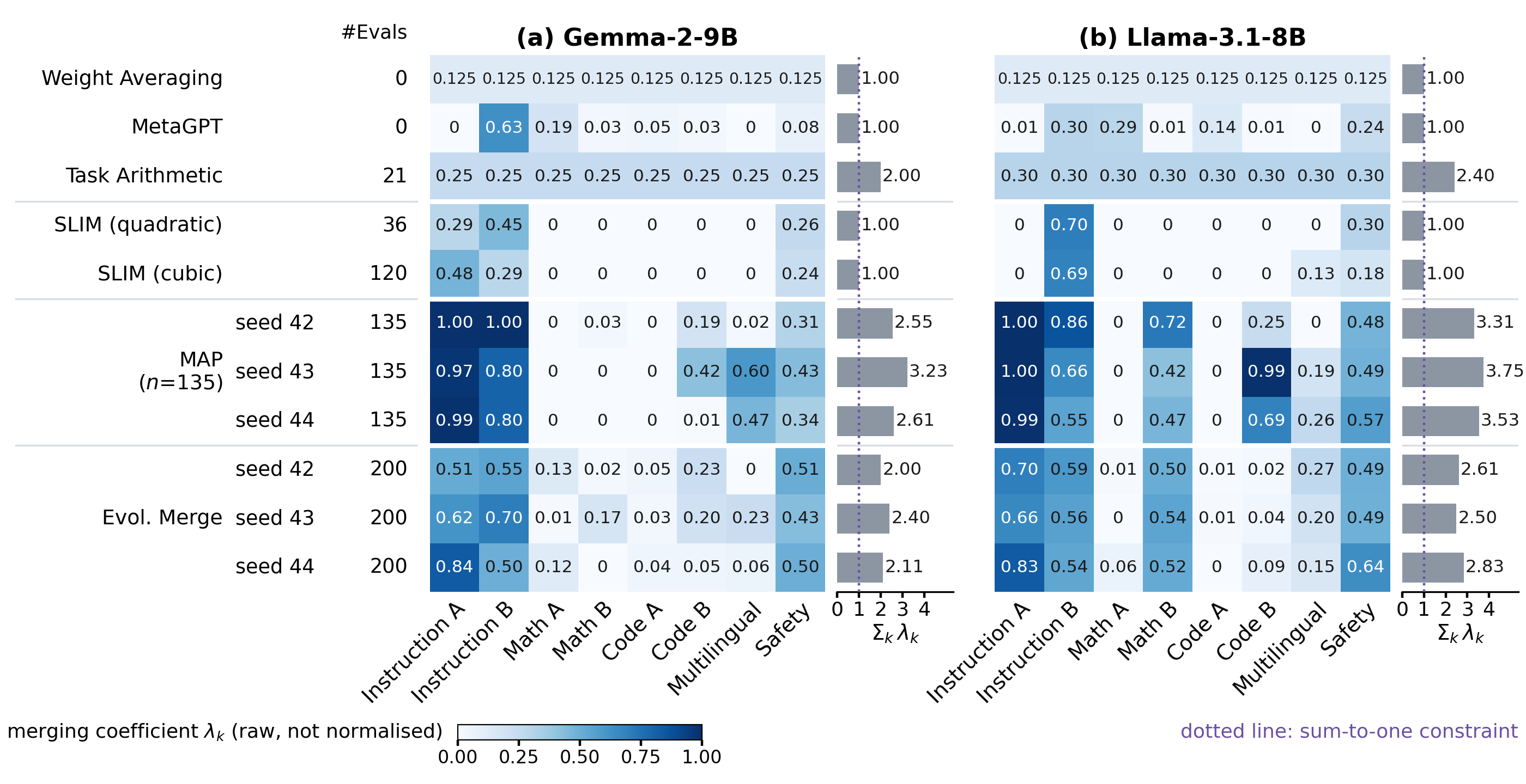
Figure 4 compares the selected coefficients and their sums. Quadratic SLIM concentrates weight on instruction and safety experts on both architectures. Thus, although we evaluate prediction at mixtures involving all eight experts, coefficient optimization can select mixtures concentrated on fewer experts. On Llama, coefficient sums range from 3.31 to 3.75 for MAP and from 2.50 to 2.83 for evolutionary merging, compared with one for SLIM. Both methods achieve higher ID AVG than SLIM at these budgets (Table 7), providing examples of higher-scoring candidates outside the simplex. The selected solutions differ in both relative allocation and overall task-vector scale.

5 Ablation Studies

5.1 Effect of Evaluation-Point Placement

We compare lattice and random evaluation points using the same quadratic function class on the simplex. For each budget $n$ , we draw $n$ of the 150 interior points from Section 4.2 without replacement and fit ID AVG by unregularized least squares (LS) or ridge regression. We repeat this procedure 1,000 times, evaluating all surrogates on the remaining $150-n$ points in each resample and keeping the 36-point lattice surrogate fixed. Ridge strength is selected by cross-validation using only the fitting points; scaling and fitting details appear in Appendix C.4.

At the matched budget of 36 evaluations, the lattice design achieves higher mean rank correlation and lower mean MAE than either random-design fit on both architectures (Table 2). Ridge reduces the random design’s mean MAE from 33.64 to 2.90 on Gemma and from 30.15 to 2.24 on Llama, compared with approximately 1.93 and 1.07 for the lattice. Among the tested budgets, the lattice’s win rate first falls below 50% at $n=60$ for Gemma and $n=105$ for Llama, against random designs fitted with either LS or ridge.

	Gemma-2-9B				Llama-3.1-8B
$n$	$\rho_{\mathrm{lattice}}$	$\rho_{\mathrm{random}}$	$\mathrm{MAE}_{\mathrm{random}}$	Lattice win	$\rho_{\mathrm{lattice}}$	$\rho_{\mathrm{random}}$	$\mathrm{MAE}_{\mathrm{random}}$	Lattice win
36	0.935	0.465 / 0.847	33.64 / 2.90	99.5 / 99.5	0.958	0.330 / 0.758	30.15 / 2.24	100.0 / 100.0
45	0.935	0.902 / 0.884	2.46 / 2.50	68.9 / 86.2	0.958	0.819 / 0.800	1.81 / 1.99	99.9 / 99.9
60	0.934	0.954 / 0.948	1.63 / 1.70	12.1 / 18.2	0.957	0.918 / 0.915	1.11 / 1.16	95.6 / 95.9
75	0.933	0.966 / 0.965	1.38 / 1.39	1.7 / 2.4	0.956	0.941 / 0.941	0.93 / 0.94	79.1 / 79.3
90	0.931	0.970 / 0.970	1.27 / 1.27	0.5 / 0.5	0.954	0.950 / 0.950	0.83 / 0.84	57.9 / 57.1
105	0.930	0.972 / 0.972	1.19 / 1.19	0.5 / 0.6	0.953	0.953 / 0.954	0.80 / 0.80	44.2 / 43.8
120	0.924	0.970 / 0.970	1.14 / 1.14	1.1 / 1.0	0.949	0.953 / 0.953	0.75 / 0.76	39.5 / 39.0

Table 2: The lattice improves AVG prediction at the matched budget of 36 evaluations. Random budgets are

n

; the lattice always uses 36. Values average 1,000 resamples with shared held-out points; pairs show LS / ridge. Lattice win is the percentage with

\rho_{\mathrm{lattice}}>\rho_{\mathrm{random}}

. Lattice MAEs average approximately 1.93 (Gemma) and 1.07 (Llama).

5.2 Effect of Surrogate Optimization

We compare quadratic SLIM with directly selecting the point with the highest measured ID AVG among the same 36 lattice points (Table 3). Most of the ID gain over vertex-only selection comes from adding equal-weight expert pairs to the candidates. Surrogate optimization provides a smaller additional ID gain; OOD AVG decreases on Gemma and increases on Llama.

		Gemma-2-9B		Llama-3.1-8B
Variant	#Evals	ID	OOD	ID	OOD
Best vertex	8	58.51	49.73	54.80	46.41
Best lattice point	36	65.37	51.85	56.56	42.93
SLIM (quadratic)	36	66.15	50.30	56.61	47.27
SLIM (cubic)	120	66.35	48.41	57.04	46.27

Table 3: Effects of evaluating expert pairs, optimizing the surrogate, and increasing its degree on merge performance. The first two rows select by measured ID AVG among eight vertices or 36 lattice points; SLIM optimizes its surrogate. #Evals counts ID evaluations for selection; OOD is held out. Bold marks column maxima.

5.3 Effect of Polynomial Degree

We compare quadratic SLIM with a cubic extension using 120 lattice points and the same simplex-constrained optimization procedure (Appendix B.4). The cubic extension yields small ID gains but lower OOD AVG on both architectures (Table 3; Figure 3). Increasing the degree and evaluation budget therefore does not consistently improve merge performance in these experiments.

6 Discussion and Limitations

Quadratic Approximation and Model Degree.

Evaluations of individual experts and equal-weight pairs support AVG prediction at mixtures of all eight experts on both architectures (Figure 1), although domain-wise fidelity varies (Table 8). Increasing the degree from quadratic to cubic raises the budget from 36 to 120 evaluations but produces small ID gains and lower OOD AVG on both architectures (Table 3). These results support quadratic approximation in the tested settings and show limited benefit from increasing the degree. When greater surrogate expressiveness improves generalization remains an open question.

Evaluation Design and Sample Efficiency.

At 36 evaluations, the lattice yields higher mean rank correlation and lower MAE than random designs, including ridge-regularized fits (Table 2). Evaluation placement therefore matters even with the surrogate class and coefficient domain fixed. The $T(T+1)/2$ count is the minimum for identifying a general quadratic on the simplex, not a universal lower bound for finding a good merge.

The Value of Surrogate Optimization.

Most ID improvement over the best individual expert comes from adding equal-weight pairs to the candidates (Table 3). Optimizing beyond the best measured lattice point yields small ID gains but lowers OOD AVG on Gemma and raises it on Llama. The surrogate enables continuous coefficient selection without further target-metric evaluations; its additional performance benefit depends on the setting.

The Role of the Simplex Constraint.

The OOD results show that the simplex contains competitive merges that generalize beyond the selection benchmarks (Figure 3). On Llama ID, MAP and evolutionary merging select higher-scoring candidates with coefficient sums above one (Figure 4). Although these comparisons do not isolate the effect of coefficient scale, they motivate varying both mixture proportions and overall task-vector scale while controlling the cost of surrogate construction.

7 Conclusion

SLIM selects LLM merging coefficients using a quadratic surrogate built from individual experts and equal-weight pairs, with the minimum evaluations required for quadratic identification on the simplex. Experiments on two architectures show accurate prediction of aggregate performance at unseen mixtures and competitive merging under limited evaluation budgets. Comparisons at a matched budget highlight evaluation-point placement as an important design choice for surrogate-based coefficient selection.

AI use statement

We used generative AI tools (ChatGPT, Claude, and Claude Code) for research ideation and discussion, literature search, writing and debugging code for experiments and figures, running experiments and analyzing results, drafting the manuscript, English editing and paraphrasing, creating figures and tables, and checking the mathematical derivations in Appendix B. We have reviewed all AI-assisted work. LLM-generated code was tested by the authors, and the resulting numerical values were verified by manual calculation or against an independent implementation. All references identified with AI assistance were checked against the original sources. We take responsibility for the final content of this work, including text, claims, and artifacts produced with the aid of generative AI.

Ethics statement

This work does not involve human subjects, personally identifiable information, or newly collected data. We are not aware of ethical concerns raised by this work beyond those associated with the publicly available models and benchmarks it uses.

Reproducibility statement

Section 3 and Algorithm 1 describe SLIM, and Appendices B.1– B.4 derive the quadratic interpolant, its uniqueness, its equivalence under domain aggregation, and the cubic extension. Appendix C.1 (Table 5) lists all base and expert checkpoints; Appendix C.2 (Table 6) specifies the benchmarks, metrics, sample counts, and prompting settings; and Appendix C.3 details the implementations of SLIM and all baselines, including random seeds, optimizer settings, and initializations. Upon acceptance, we will release our code together with the measured scores used in our experiments, including those at the lattice design points and the 150 held-out mixtures. These measurements allow the surrogate-fidelity results and SLIM’s coefficient selection to be reproduced without re-evaluating merged models.

Acknowledgments

This work was supported by JST SPRING (Grant Number JPMJSP2108) and JSPS KAKENHI (Grant Number 23H04974).

References

Akiba et al. (2025) T. Akiba, M. Shing, Y. Tang, Q. Sun, and D. Ha Evolutionary optimization of model merging recipes. Nature Machine Intelligence 7 (2), pp. 195–204. Cited by: §1, §2, §4.1.
Austin et al. (2021) J. Austin, A. Odena, M. Nye, M. Bosma, H. Michalewski, D. Dohan, E. Jiang, C. Cai, M. Terry, Q. Le, et al. Program synthesis with large language models. arXiv preprint arXiv:2108.07732. Cited by: Table 6.
Burchell et al. (2024) L. Burchell, J. Maillard, A. Anastasopoulos, C. Federmann, P. Koehn, and S. Wang Findings of the WMT 2024 shared task of the open language data initiative. In Proceedings of the Ninth Conference on Machine Translation, pp. 110–117. Cited by: Table 6.
Chen et al. (2021) M. Chen, J. Tworek, H. Jun, Q. Yuan, H. P. D. O. Pinto, J. Kaplan, H. Edwards, Y. Burda, N. Joseph, G. Brockman, et al. Evaluating large language models trained on code. arXiv preprint arXiv:2107.03374. Cited by: Table 6.
Cobbe et al. (2021) K. Cobbe, V. Kosaraju, M. Bavarian, M. Chen, H. Jun, L. Kaiser, M. Plappert, J. Tworek, J. Hilton, R. Nakano, et al. Training verifiers to solve math word problems. arXiv preprint arXiv:2110.14168. Cited by: Table 6.
Cornell (2002) J. A. Cornell Experiments with mixtures: designs, models, and the analysis of mixture data. 3rd edition, John Wiley & Sons. Cited by: §2.
Dubois et al. (2024) Y. Dubois, B. Galambosi, P. Liang, and T. B. Hashimoto Length-controlled alpacaeval: a simple way to debias automatic evaluators. arXiv preprint arXiv:2404.04475. Cited by: Table 6.
Gemma Team et al. (2024) Gemma Team, M. Riviere, S. Pathak, P. G. Sessa, C. Hardin, S. Bhupatiraju, L. Hussenot, T. Mesnard, B. Shahriari, A. Ramé, et al. Gemma 2: improving open language models at a practical size. arXiv preprint arXiv:2408.00118. Cited by: §C.1, §1, §4.1.
Grattafiori et al. (2024) A. Grattafiori, A. Dubey, A. Jauhri, A. Pandey, A. Kadian, A. Al-Dahle, A. Letman, A. Mathur, A. Schelten, A. Vaughan, et al. The llama 3 herd of models. arXiv preprint arXiv:2407.21783. Cited by: §C.1, §1, §4.1.
Han et al. (2024) S. Han, K. Rao, A. Ettinger, L. Jiang, B. Y. Lin, N. Lambert, Y. Choi, and N. Dziri Wildguard: open one-stop moderation tools for safety risks, jailbreaks, and refusals of llms. Advances in neural information processing systems 37, pp. 8093–8131. Cited by: Table 6.
He et al. (2025) Y. He, S. Zeng, Y. Hu, R. Yang, T. Zhang, and H. Zhao MergeBench: a benchmark for merging domain-specialized LLMs. In The Thirty-ninth Annual Conference on Neural Information Processing Systems Datasets and Benchmarks Track, External Links: Link Cited by: §C.1.
Hendrycks et al. (2021) D. Hendrycks, C. Burns, S. Kadavath, A. Arora, S. Basart, E. Tang, D. Song, and J. Steinhardt Measuring mathematical problem solving with the math dataset. arXiv preprint arXiv:2103.03874. Cited by: Table 6.
Ilharco et al. (2023) G. Ilharco, M. T. Ribeiro, M. Wortsman, L. Schmidt, H. Hajishirzi, and A. Farhadi Editing models with task arithmetic. In The Eleventh International Conference on Learning Representations, External Links: Link Cited by: §1, §2, §4.1.
Kiefer (1961) J. Kiefer Optimum designs in regression problems, ii. The Annals of Mathematical Statistics 32 (1), pp. 298–325. Cited by: §2.
Li et al. (2026) B. Li, Z. Di, Y. Yang, H. Qian, P. Yang, H. Hao, K. Tang, and A. Zhou It’s morphing time: unleashing the potential of multiple llms via multiobjective optimization. IEEE Transactions on Evolutionary Computation 30 (4), pp. 1699–1713. External Links: Document Cited by: §2.
Li et al. (2025) L. Li, T. Zhang, Z. Bu, S. Wang, H. He, J. Fu, Y. Wu, J. Bian, Y. Chen, and Y. Bengio MAP: low-compute model merging with amortized pareto fronts via quadratic approximation. In International Conference on Learning Representations, Y. Yue, A. Garg, N. Peng, F. Sha, and R. Yu (Eds.), Vol. 2025, pp. 65032–65064. External Links: Link Cited by: §1, §1, §2, §3.2, §4.1.
Lightman et al. (2024) H. Lightman, V. Kosaraju, Y. Burda, H. Edwards, B. Baker, T. Lee, J. Leike, J. Schulman, I. Sutskever, and K. Cobbe Let’s verify step by step. In International Conference on Learning Representations, Vol. 2024, pp. 39578–39601. Cited by: Table 6.
Mao and Du (2026) Y. Mao and H. Du Data mixing as mixture experiment: response surface methodology and optimal design for large language model pretraining. arXiv preprint arXiv:2608.23922. Cited by: §2.
Mazeika et al. (2024) M. Mazeika, L. Phan, X. Yin, A. Zou, Z. Wang, N. Mu, E. Sakhaee, N. Li, S. Basart, B. Li, D. Forsyth, and D. Hendrycks HarmBench: a standardized evaluation framework for automated red teaming and robust refusal. In Proceedings of the 41st International Conference on Machine Learning, R. Salakhutdinov, Z. Kolter, K. Heller, A. Weller, N. Oliver, J. Scarlett, and F. Berkenkamp (Eds.), Proceedings of Machine Learning Research, Vol. 235, pp. 35181–35224. External Links: Link Cited by: Table 6.
Mencattini et al. (2025) T. Mencattini, A. R. Minut, D. Crisostomi, A. Santilli, and E. Rodolà MERGE ${}^{3}$ : efficient evolutionary merging on consumer-grade gpus. In Proceedings of the 42nd International Conference on Machine Learning (ICML), External Links: Link Cited by: §2.
NLLB Team (2024) NLLB Team Scaling neural machine translation to 200 languages. Nature 630, pp. 841–846. External Links: Document Cited by: Table 6.
Scheffé (1958) H. Scheffé Experiments with mixtures. Journal of the Royal Statistical Society: Series B (Methodological) 20 (2), pp. 344–360. Cited by: §B.1, §B.4, §1, §2, §3.2, §3.2.
Song and Zheng (2026) M. Song and M. Zheng Model merging in the era of large language models: methods, applications, and future directions. arXiv preprint arXiv:2603.09938. Cited by: §1, §2.
Su and Geiping (2025) G. Su and J. Geiping Fine, i’ll merge it myself: a multi-fidelity framework for automated model merging. arXiv preprint arXiv:2502.04030. Cited by: §1, §2, §2.
Wortsman et al. (2022) M. Wortsman, G. Ilharco, S. Y. Gadre, R. Roelofs, R. Gontijo-Lopes, A. S. Morcos, H. Namkoong, A. Farhadi, Y. Carmon, S. Kornblith, et al. Model soups: averaging weights of multiple fine-tuned models improves accuracy without increasing inference time. In International conference on machine learning, pp. 23965–23998. Cited by: §1, §4.1.
Yadav et al. (2023) P. Yadav, D. Tam, L. Choshen, C. A. Raffel, and M. Bansal Ties-merging: resolving interference when merging models. Advances in neural information processing systems 36, pp. 7093–7115. Cited by: §2.
Yang et al. (2026) E. Yang, L. Shen, G. Guo, X. Wang, X. Cao, J. Zhang, and D. Tao Model merging in llms, mllms, and beyond: methods, theories, applications, and opportunities. ACM Comput. Surv. 58 (8), pp. 216–257. Cited by: §1, §2.
Yang et al. (2024) E. Yang, Z. Wang, L. Shen, S. Liu, G. Guo, X. Wang, and D. Tao AdaMerging: adaptive model merging for multi-task learning. The Twelfth International Conference on Learning Representations. Cited by: §2.
Yu et al. (2024) L. Yu, B. Yu, H. Yu, F. Huang, and Y. Li Language models are super mario: absorbing abilities from homologous models as a free lunch. In Forty-first International Conference on Machine Learning, Cited by: §2.
Zhou et al. (2023) J. Zhou, T. Lu, S. Mishra, S. Brahma, S. Basu, Y. Luan, D. Zhou, and L. Hou Instruction-following evaluation for large language models. arXiv preprint arXiv:2311.07911. Cited by: Table 6.
Zhou et al. (2024) Y. Zhou, L. Song, B. Wang, and W. Chen Metagpt: merging large language models using model exclusive task arithmetic. In Proceedings of the 2024 Conference on Empirical Methods in Natural Language Processing, pp. 1711–1724. Cited by: §C.3, §1, §2, §4.1.

Appendix Contents

Appendix A Notation

Symbol	Meaning
$T$	Number of expert models.
$\theta_{\mathrm{pre}},\theta_{k}$	Parameters of the shared base model and expert $k$ .
$\tau_{k}$	Task vector $\theta_{k}-\theta_{\mathrm{pre}}$ .
$\lambda,\lambda_{k}$	Merging coefficient vector and its $k$ -th component.
$\theta(\lambda)$	Merged parameters $\theta_{\mathrm{pre}}+\sum_{k}\lambda_{k}\tau_{k}$ .
$\Lambda$	General feasible set of merging coefficients.
$\Delta^{T-1}$	Coefficient simplex: $\lambda_{k}\geq 0$ and $\sum_{k}\lambda_{k}=1$ .
$e_{k}$	$k$ -th standard basis vector; the vertex corresponding to expert $k$ .
$\mathcal{D}$	Evaluation design consisting of the vertices and edge midpoints.
$M(\lambda)$	Measured target metric of $\theta(\lambda)$ ; AVG in the experiments.
$M_{k},M_{ij}$	Measurements $M(e_{k})$ and $M((e_{i}+e_{j})/2)$ .
$\widehat{M}(\lambda)$	Quadratic interpolant constructed from measurements on $\mathcal{D}$ .
$q,\beta_{k},\beta_{ij}$	A quadratic in canonical mixture form and its linear and pairwise coefficients.
$\varphi_{a}(\lambda)$	Interpolation basis function associated with design point $a\in\mathcal{D}$ .
$\lambda^{\star}$	A maximizer of $M$ over $\Lambda$ .
$\widehat{\lambda}$	Coefficients returned by numerical optimization of $\widehat{M}$ over $\Delta^{T-1}$ .
$D,M_{d},w_{d}$	Number of domains, domain- $d$ metric, and its fixed aggregation weight; $w_{d}=1/D$ for AVG.
$\widehat{M}_{d}$	Interpolant of domain- $d$ measurements on $\mathcal{D}$ .
$n$	Number of evaluation points used by MAP or a random-design surrogate.

Table 4: Symbols defining the merging coefficients, target metric, and surrogate construction.

Appendix B Additional Details on the Methods

B.1 Derivation and Uniqueness

On the simplex, $1=\sum_{k}\lambda_{k}$ and $\lambda_{k}^{2}=\lambda_{k}-\sum_{j\neq k}\lambda_{k}\lambda_{j}$ . Thus, constant and squared terms can be absorbed into linear and pairwise terms, giving the canonical mixture form in Eq. 4 (Scheffé, 1958).

At each vertex, interpolation requires $\beta_{k}=q(e_{k})=M_{k}$ . At the midpoint of experts $i$ and $j$ ,

q\left(\frac{e_{i}+e_{j}}{2}\right)=\frac{\beta_{i}+\beta_{j}}{2}+\frac{\beta_{ij}}{4}=M_{ij},

(9)

\beta_{ij}=4M_{ij}-2M_{i}-2M_{j}.

(10)

The vertex and midpoint values uniquely determine all $T+\binom{T}{2}$ coefficients. Conversely, each evaluation supplies one linear constraint on these coefficients, so fewer evaluations cannot identify an unrestricted member of this quadratic space.

Substituting $\beta_{k}=M_{k}$ and Eq. 10 into Eq. 4 gives

	$\displaystyle q(\lambda)$	$\displaystyle=\sum_{k}M_{k}\lambda_{k}+\sum_{i<j}(4M_{ij}-2M_{i}-2M_{j})\lambda_{i}\lambda_{j}$
		$\displaystyle=\sum_{k}M_{k}\lambda_{k}+\sum_{i<j}4M_{ij}\lambda_{i}\lambda_{j}-2\sum_{i<j}(M_{i}+M_{j})\lambda_{i}\lambda_{j}$
		$\displaystyle=\sum_{k}M_{k}\lambda_{k}+\sum_{i<j}4M_{ij}\lambda_{i}\lambda_{j}-2\left(\sum_{i<j}M_{i}\lambda_{i}\lambda_{j}+\sum_{i<j}M_{j}\lambda_{i}\lambda_{j}\right).$
Regrouping the pairwise terms by expert index $k$ gives
	$\displaystyle q(\lambda)$	$\displaystyle=\sum_{k}M_{k}\lambda_{k}+\sum_{i<j}4M_{ij}\lambda_{i}\lambda_{j}-2\sum_{k}M_{k}\lambda_{k}\left(\sum_{\ell>k}\lambda_{\ell}+\sum_{\ell<k}\lambda_{\ell}\right)$
		$\displaystyle=\sum_{k}M_{k}\lambda_{k}+\sum_{i<j}4M_{ij}\lambda_{i}\lambda_{j}-2\sum_{k}M_{k}\lambda_{k}\sum_{\ell\neq k}\lambda_{\ell}.$
The simplex constraint implies $\sum_{\ell\neq k}\lambda_{\ell}=\sum_{\ell}\lambda_{\ell}-\lambda_{k}=1-\lambda_{k}$ . Therefore,
	$\displaystyle q(\lambda)$	$\displaystyle=\sum_{k}M_{k}\lambda_{k}+\sum_{i<j}4M_{ij}\lambda_{i}\lambda_{j}-2\sum_{k}M_{k}\lambda_{k}(1-\lambda_{k})$
		$\displaystyle=\sum_{k}\lambda_{k}(2\lambda_{k}-1)M_{k}+\sum_{i<j}4\lambda_{i}\lambda_{j}M_{ij},$

which is Eq. 7.

B.2 Linearity under Domain Aggregation

For domain metrics $M_{d}$ and fixed weights $w_{d}$ , define

M(\lambda)=\sum_{d=1}^{D}w_{d}M_{d}(\lambda).

(11)

AVG corresponds to $w_{d}=1/D$ . Let $\varphi_{a}$ denote the basis function in Eq. 7 associated with design point $a\in\mathcal{D}$ . Since these functions do not depend on the measured values,

	$\displaystyle\widehat{M}(\lambda)$	$\displaystyle=\sum_{a\in\mathcal{D}}\varphi_{a}(\lambda)\sum_{d=1}^{D}w_{d}M_{d}(a)$
		$\displaystyle=\sum_{d=1}^{D}w_{d}\sum_{a\in\mathcal{D}}\varphi_{a}(\lambda)M_{d}(a)=\sum_{d=1}^{D}w_{d}\widehat{M}_{d}(\lambda).$

Thus, interpolating aggregated measurements and aggregating domain-wise interpolants give the same surrogate. No additional model evaluations are needed when the domain scores are recorded at the same design points.

B.3 SLIM Algorithm

Algorithm 1 SLIM: Simplex-Lattice Interpolation Merging

1: Base parameters

\theta_{\mathrm{pre}}

; task vectors

\{\tau_{k}\}_{k=1}^{T}

; target metric

M

2: Merge coefficients

\widehat{\lambda}

3: Construct

\mathcal{D}

using Eq. 5

4: for all

\lambda\in\mathcal{D}

5: Form

\theta(\lambda)

using Eq. 1

6: Evaluate the model and store

M(\lambda)

7: end for

8: Construct

\widehat{M}

using Eq. 7

9: Numerically maximize

\widehat{M}

over

\Delta^{T-1}

to obtain

\widehat{\lambda}

10: return

\widehat{\lambda}

B.4 Cubic Extension for the Degree Ablation

For the polynomial-degree ablation, we construct a cubic interpolant on the same coefficient simplex using the $\{T,3\}$ simplex-lattice design (Scheffé, 1958):

\mathcal{A}_{3}=\left\{\alpha\in\mathbb{Z}_{\geq 0}^{T}\,\middle|\,\sum_{k=1}^{T}\alpha_{k}=3\right\},\qquad\mathcal{D}_{3}=\left\{\frac{\alpha}{3}\,\middle|\,\alpha\in\mathcal{A}_{3}\right\}.

(12)

Figure 2 illustrates the quadratic and cubic designs for $T=3$ .

The design contains the vertices, two points per expert pair with weights $(2/3,1/3)$ and $(1/3,2/3)$ , and the equal-weight mixture of each expert triple. Its size is

|\mathcal{D}_{3}|=T+2\binom{T}{2}+\binom{T}{3}=\binom{T+2}{3},

(13)

giving $8+56+56=120$ evaluations for $T=8$ .

Using the measured ID AVG at each design point, we construct

	$\displaystyle\widehat{M}_{3}(\lambda)$	$\displaystyle=\sum_{\alpha\in\mathcal{A}_{3}}\varphi^{(3)}_{\alpha}(\lambda)\,M(\alpha/3),$		(14)
	$\displaystyle\varphi^{(3)}_{\alpha}(\lambda)$	$\displaystyle=\prod_{k=1}^{T}\prod_{\ell=0}^{\alpha_{k}-1}\frac{3\lambda_{k}-\ell}{\alpha_{k}-\ell},$		(14)

where an empty product equals one.

At a design point $\gamma/3$ , the basis function equals one if $\gamma=\alpha$ . Otherwise, some $\gamma_{k}<\alpha_{k}$ , making a factor in the product zero. Thus, $\widehat{M}_{3}$ reproduces all measured values. The number of cardinal basis functions equals the dimension $\binom{T+2}{3}$ of polynomials of degree at most three on the simplex, so the interpolant is unique in this space.

We numerically maximize $\widehat{M}_{3}$ over $\Delta^{T-1}$ using the same SLSQP settings and initializations as quadratic SLIM (Appendix C.3). This optimization requires no further model evaluations, leaving the budget at $|\mathcal{D}_{3}|=120$ for $T=8$ .

Appendix C Additional Details on Experiments

C.1 Models and Checkpoints

Table 5 lists the checkpoints used for Gemma-2-9B (Gemma Team et al., 2024) and Llama-3.1-8B (Grattafiori et al., 2024). Each expert set contains five domain-specific checkpoints from MergeBench (He et al., 2025) and three additional checkpoints: Instruction B, Math B, and Code B. Instruction B is the official instruction-tuned model.

Role	Hugging Face identifier
Gemma-2-9B
Base	google/gemma-2-9b
Instruction A	MergeBench/gemma-2-9b_instruction
Instruction B	google/gemma-2-9b-it
Math A	MergeBench/gemma-2-9b_math
Math B	POME-OPTIM/Gemma2-9B-MetaMathQA
Code A	MergeBench/gemma-2-9b_coding
Code B	testmoto/gemma-2-9b-synthetic_coding
Multilingual	MergeBench/gemma-2-9b_multilingual
Safety	MergeBench/gemma-2-9b_safety
Llama-3.1-8B
Base	meta-llama/Llama-3.1-8B
Instruction A	MergeBench/Llama-3.1-8B_instruction
Instruction B	meta-llama/Llama-3.1-8B-Instruct
Math A	MergeBench/Llama-3.1-8B_math
Math B	pmahdavi/Llama-3.1-8B-math-reasoning
Code A	MergeBench/Llama-3.1-8B_coding
Code B	pmahdavi/Llama-3.1-8B-coding
Multilingual	MergeBench/Llama-3.1-8B_multilingual
Safety	MergeBench/Llama-3.1-8B_safety
External evaluator
Refusal classifier	allenai/wildguard

Table 5: Shared bases and eight experts per architecture, with identifiers linked to their releases. A and B distinguish experts in the same domain. WildGuard is the external evaluator and is not merged.

C.2 Benchmarks and Evaluation Protocol

Table 6 provides benchmark sources and evaluation settings. ID benchmarks are used for coefficient selection and the reported ID results; OOD benchmarks are held out from selection.

Benchmark	Role	Examples	Shots	Scoring
IFEval (Zhou et al., 2023)	ID	541	0	Prompt-level strict accuracy
AlpacaEval 2.0 (Dubois et al., 2024)	OOD	805	0	Length-controlled win rate
GSM8K-CoT (Cobbe et al., 2021)	ID	1,319	8	Strict-match exact match
MATH-500 (Hendrycks et al., 2021; Lightman et al., 2024)	OOD	500	4	Verified accuracy (math_verify)
MBPP (Austin et al., 2021)	ID	500	3	pass@1
HumanEval (Chen et al., 2021)	OOD	164	0	pass@1
FLORES+ dev (NLLB Team, 2024; Burchell et al., 2024)	ID	$100\times 8$	0	chrF2
FLORES+ devtest	OOD	$1{,}012\times 8$	0	chrF2
HarmBench (Mazeika et al., 2024)	ID	320	0	Refuse-to-answer rate
WildGuardTest (Han et al., 2024)	OOD	749	0	Refuse-to-answer rate

Table 6: Sample counts, prompting, and scoring for ID selection and held-out OOD evaluation. Shots denotes in-context examples. FLORES+ counts are sentences per target language times eight languages. Refusal rates use WildGuard.

We use openlanguagedata/flores_plus for translation from English into German, French, Spanish, Chinese, Russian, Arabic, Hindi, and Japanese. ID evaluation reuses a fixed subset of 100 dev sentences per target language (seed 42); OOD evaluation uses all 1,012 devtest sentences per language. The multilingual score is the mean chrF2 across these eight languages. WildGuardTest has 749 evaluated examples after five entries with missing values are excluded. Accuracy and pass@1 scores are multiplied by 100; chrF2, refusal rates, and the AlpacaEval win rate are expressed on the same 0–100 scale.

Merged candidates inherit the base model’s configuration and tokenizer, with benchmark-specific prompt formatting applied consistently. The lm-eval tasks and FLORES+ use raw prompts; AlpacaEval uses the architecture’s Instruct chat template, and safety evaluation uses a shared chat format. Simplex vertices follow this pipeline: their weights equal those of the corresponding experts, but their scores can differ from evaluations using each expert’s native tokenizer, prompts, and generation settings.

C.3 Coefficient-Selection Implementations

MetaGPT.

MetaGPT (Zhou et al., 2024) computes $\lambda_{k}=\|\tau_{k}\|_{2}^{2}/\sum_{j}\|\tau_{j}\|_{2}^{2}$ from the full task vectors. This rule gives nonnegative coefficients summing to one and requires no target-metric evaluations.

MAP.

For each seed, we construct one sequence of 135 coefficient vectors. With zero-based indexing, indices 0–7 are $e_{1},\ldots,e_{8}$ ; indices 8–134 are 127 independent draws from $\mathcal{U}([0,1]^{8})$ , with all coordinates sampled independently. We initialize np.random.default_rng(seed) and generate these coordinates with uniform(0, 1). The fit at budget $n\in\{45,90,135\}$ uses the first $n$ points, so all three budgets contain the eight vertices and form nested samples.

For $T=8$ , each surrogate’s quadratic component has $(T+1)(T+2)/2=45$ coefficients. The budgets of 45, 90, and 135 evaluations are one, two, and three times this count; 90 is the released implementation’s default. We adapt the released implementation in three ways. First, we divide scores by 100 to match the sigmoid output range, corresponding to a bounded-response model on the original 0–100 score scale. Second, we replace all-ones surrogate parameter initialization with zeros to avoid initial sigmoid saturation. Third, we replace the released code’s search bounds $[-3,3]^{8}$ with $[0,1]^{8}$ so that optimization remains within the domain from which the surrogate-fitting points are sampled. All reported MAP results use these adjustments to the released implementation. NSGA-III in DEAP uses a population of 100 for 150 generations over $x\in[0,1]^{8}$ . We evaluate the surrogates at $x$ , select the vector with the highest predicted AVG from the approximate Pareto front, and use that same vector directly as the merging coefficients, $\lambda=x$ . The sigmoid is applied only to the surrogate outputs, not to the merging coefficients. This selection requires no additional target-metric evaluations.

Evolutionary merging.

For $T=8$ , CMA-ES uses a population size of $4+\lfloor 3\ln T\rfloor=10$ , an initial mean of 0.5 in every coordinate, an initial step size of $1/6$ , and bounds $[0,1]^{8}$ . For each seed, we use a single run of 20 generations and report ID scores after every generation. The OOD evaluation checkpoints of 10, 30, 40, 50, 100, 150, and 200 cumulative evaluations correspond to generations 1, 3, 4, 5, 10, 15, and 20, respectively. At each checkpoint, we report the ID and OOD scores of the candidate with the highest measured ID AVG among all candidates evaluated so far.

SLIM.

We interpolate the measured ID AVG directly; by linearity, this is equivalent to averaging the domain-wise interpolants (Appendix B.2). For both quadratic and cubic variants, SLSQP uses analytic gradients, $\sum_{k}\lambda_{k}=1$ , bounds $0\leq\lambda_{k}\leq 1$ , ftol $=10^{-12}$ , and at most 1,000 iterations per initialization. The 20 initializations comprise the barycenter, eight points near the vertices, and 11 random simplex points generated with seed 42. We retain the converged solution with the highest surrogate value. Given the measurements and these fixed initializations, the procedure is deterministic and uses no additional target-metric evaluations. The cubic extension is defined in Appendix B.4.

C.4 Random-Design Fits

The evaluation-placement ablation uses the same Scheffé basis for LS and ridge: eight linear terms and 28 pairwise terms, with no explicit intercept. For ridge, each feature is divided by its root mean square without centering. We select $\alpha\in\{10^{-4},10^{-3},\ldots,10^{2}\}$ by five-fold cross-validation on the $n$ fitting points, minimizing mean squared error and recomputing feature scales within each training fold. The remaining $150-n$ points are used only to assess prediction fidelity.

C.5 Numerical Results for Figure 3

Table 7 gives the numerical results underlying Figure 3. All coefficients are selected using ID evaluations only.

		Gemma-2-9B			Llama-3.1-8B
Method	#Evals	GPU-h	ID AVG	OOD AVG	GPU-h	ID AVG	OOD AVG
Weight Averaging	0	0	50.1	40.0	0	43.3	33.2
MetaGPT	0	0	62.4	50.6	0	47.1	35.5
Task Arithmetic	21	3.0	52.0	39.5	2.7	50.2	37.6
Evol. Merge (gen $=$ 1)	10	1.4	$51.5_{\pm 0.8}$	$32.7_{\pm 1.1}$	1.3	$54.0_{\pm 1.0}$	$38.3_{\pm 0.4}$
Evol. Merge (gen $=$ 3)	30	4.1	$60.1_{\pm 0.8}$	$38.6_{\pm 1.3}$	3.9	$58.4_{\pm 1.7}$	$42.1_{\pm 2.0}$
Evol. Merge (gen $=$ 4)	40	5.4	$60.7_{\pm 0.5}$	$40.7_{\pm 3.1}$	5.0	$58.9_{\pm 1.9}$	$41.1_{\pm 1.1}$
Evol. Merge (gen $=$ 5)	50	6.7	$63.5_{\pm 1.8}$	$45.5_{\pm 4.4}$	6.2	$60.0_{\pm 1.9}$	$43.3_{\pm 1.3}$
Evol. Merge (gen $=$ 10)	100	13.8	$65.3_{\pm 2.1}$	$46.9_{\pm 4.4}$	11.9	$63.2_{\pm 0.1}$	$45.8_{\pm 2.2}$
Evol. Merge (gen $=$ 15)	150	20.4	$66.4_{\pm 2.4}$	$48.7_{\pm 0.6}$	17.6	$63.9_{\pm 0.6}$	$47.2_{\pm 1.5}$
Evol. Merge (gen $=$ 20)	200	26.8	$\mathbf{67.4}_{\pm 1.2}$	$49.0_{\pm 0.9}$	23.2	$\mathbf{64.6}_{\pm 0.6}$	$45.5_{\pm 1.9}$
MAP ( $n=45$ )	45	6.3	$56.7_{\pm 4.2}$	$41.2_{\pm 5.6}$	5.5	$47.4_{\pm 1.8}$	$36.7_{\pm 2.1}$
MAP ( $n=90$ )	90	12.4	$58.3_{\pm 2.6}$	$47.5_{\pm 2.7}$	11.1	$57.6_{\pm 5.9}$	$43.1_{\pm 7.0}$
MAP ( $n=135$ )	135	18.5	$61.2_{\pm 1.5}$	$50.6_{\pm 0.4}$	16.7	$60.4_{\pm 1.2}$	$45.3_{\pm 2.6}$
SLIM (quadratic)	36	5.2	66.2	50.3	3.9	56.6	47.3
SLIM (cubic)	120	16.4	66.4	48.4	12.9	57.0	46.3

Table 7: ID and held-out OOD performance across coefficient-selection budgets (

T=8

; Figure 3). AVG is the unweighted mean of five domain scores on a 0–100 scale. MAP and evolutionary merging report mean

\pm

standard deviation over three seeds; their GPU-hours are means. Costs cover coefficient selection per run, excluding final reporting and fidelity measurements. Zero cost denotes no target-metric evaluations. Bold marks the highest AVG in each column before rounding. On Gemma OOD, MetaGPT (50.62) and MAP with

n=135

(50.60) both round to 50.6. The cubic variant is a degree ablation.

C.6 Domain-wise Surrogate Fidelity

Table 8 reports fidelity on the same 150 held-out mixtures as Figure 1. The interquartile range (IQR) of measured scores provides context for the MAE. The AVG row evaluates predictions of the aggregate objective; it is not an average of the domain-wise fidelity statistics.

	Gemma-2-9B			Llama-3.1-8B
Domain	$\rho$	MAE	IQR	$\rho$	MAE	IQR
Instruction	0.97	2.60	15.9	0.96	2.46	10.9
Math	$-0.24$	4.88	5.0	0.85	2.33	6.5
Coding	0.86	1.89	4.2	0.70	1.93	3.9
Multilingual	0.63	1.40	1.1	0.56	1.22	0.6
Safety	0.94	9.20	47.2	0.95	4.39	19.9
AVG	0.936	1.93	10.1	0.959	1.07	4.6

Table 8: AVG is accurately predicted despite variation in domain-wise fidelity. On 150 held-out mixtures, Spearman’s

\rho

compares predicted and measured rankings; MAE and the IQR of measured scores are in score points. All interpolants use the same 36 construction evaluations.

C.7 Quadratic Interpolation along Simplex Edges

For each expert pair $(i,j)$ , we consider $\lambda(t)=(1-t)e_{i}+te_{j}$ for $t\in[0,1]$ . The quadratic interpolant uses measurements at $t=0,1/2,1$ . We assess its predictions at $t=1/3,2/3$ , giving 56 held-out points across 28 edges per architecture. These points are excluded from quadratic surrogate construction and coefficient selection, although they belong to the cubic design. All scores are measured on the ID benchmarks.

MAE is 1.74 on Gemma and 1.38 on Llama, with maximum absolute errors of 8.08 and 4.28, respectively. The curves show useful interpolation overall, with localized deviations. This analysis complements the interior-mixture evaluation in Section 4.2.