1]Georgia Institute of Technology 2]Lawrence Berkeley National Lab 3]KTH Royal Institute of Technology 4]Nordita 5]International Computer Science Institute \correspondence; ; and

Variational Streaming Flow: Probabilistic Forecasting in Physical Time

Hans Hao-Hsun Hsu Minseon Gwak Soon Hoe Lim^*
Pan Li N. Benjamin Erichson Affiliation: [ Affiliation: [ Affiliation: [ Affiliation: [ Affiliation: [ Email: shlim@kth.se Email: panli@gatech.edu Email: erichson@lbl.gov

Abstract

Probabilistic forecasting is important for predicting complex dynamical systems because intrinsic randomness and incomplete observations can cause the same observed state to evolve into multiple plausible futures. While flow matching is a flexible approach for probabilistic forecasting, it is computationally expensive. Streaming flow (SF) reformulates this approach to model temporal evolution efficiently by learning a continuous velocity field directly in physical time. However, SF learns a deterministic velocity field. Thus, it provides only a single future trajectory for a given fixed initial state and observation history. To overcome this limitation, we introduce Variational Streaming Flow (VSF). Our approach learns a latent distribution that is conditioned on the dynamics of interest. In turn, this enables probabilistic forecasting. Importantly, we retain the computational efficiency of SF by generating in physical time. Across deterministic and stochastic dynamical systems, VSF demonstrates superior predictive accuracy and distributional fidelity. We demonstrate the advantage for both long-horizon rollouts exceeding 1,000 steps, and settings with bifurcating dynamics. Moreover, VSF can be integrated into existing Joint-Embedding Predictive Architecture (JEPA)-based world models as a plug-and-play predictor to improve temporal dynamics and goal-directed success rate in navigation, motion planning, and manipulation. Our code is available at https://github.com/hans66hsu/VSF-forecasting.

^*^*footnotetext: Work done while visiting ICSI/UC Berkeley.

Figure 1: Our variational streaming flow approach obtains lower forecasting error over long rollouts than standard streaming flow. Left: continuous ranked probability score (CRPS) on the deterministic double pendulum. Right: energy distance (ED) on the partially observed Rössler system.

1 Introduction

Forecasting dynamical systems over long horizons remains challenging. Even when the dynamics are deterministic, small measurement or prediction errors can compound over a long rollout (Zhang and Gilpin, 2025). Predicting the entire future trajectory at once can avoid this recursive error accumulation, but this becomes an increasingly difficult learning task as the forecast horizon grows. Many real-world systems are also stochastic, which means that there can be many different future trajectories for the same sequence of observations (Pfister et al., 2026). For example, in weather forecasting (Feng and Fu, 2013; Sandu et al., 2019; Price et al., 2025), unresolved atmospheric processes can lead to different storm tracks from similar observations. In these settings, predicting just a single trajectory is insufficient for forecasting or planning. This motivates probabilistic forecasts that represent a distribution over possible futures (Chua et al., 2018; Porcher et al., 2026).

Flow matching provides a flexible way to learn probabilistic forecasts over entire future trajectories (Lipman et al., 2024; Kollovieh et al., 2025); see App. A for related work. However, generating a forecast requires integrating a learned vector field along an auxiliary flow time that is separate from the physical evolution of the system. Streaming and physical-time formulations instead evolve the predicted state directly through physical time, making long-horizon forecasting more efficient (Jiang et al., 2025; Liu et al., 2026). However, a standard non-latent physical-time model with a deterministic velocity field produces only one future from a fixed observed state.

To address this limitation, we introduce Variational Streaming Flow (VSF), a probabilistic extension of physical-time flow forecasting. VSF augments the physical-time velocity field with a latent variable that is sampled once for each forecast and kept fixed throughout the rollout. This preserves the computational efficiency of streaming flow (SF) while improving long-horizon forecasting accuracy, as shown in Fig. 1. Different latent samples can also generate different future trajectories from the same observed state, allowing VSF to represent multiple possible futures. During training, we use an encoder to infer the latent variable from the observed future transition and regularize its distribution toward a fixed prior (Guo and Schwing, 2025; Eijkelboom et al., 2024). At inference, we only need to sample a latent from the prior and keep it fixed throughout the rollout.

Refer to caption — Figure 2: VSF can serve as a predictor in a JEPA-based world model. We replace the deterministic autoregressive predictor with an action-conditioned VSF predictor while keeping the JEPA encoder and CEM planner fixed. The encoder maps the current and goal observations into latent space. For each action sequence, VSF samples multiple latents and rolls out future trajectories. CEM compares the predicted terminal states with the goal representation and uses these costs to select a plan.

We evaluate VSF on deterministic and partially observed stochastic dynamical systems, including chaotic systems and settings with branching futures, testing both predictive accuracy and distributional fidelity. On deterministic systems, VSF improves long-horizon predictive accuracy over DeepAR (Salinas et al., 2020), diffusion- and flow-based forecasters, SF (Jiang et al., 2025), and Chronos-2 (Ansari et al., 2025). On stochastic Rössler and Lorenz systems, VSF more accurately recovers the conditional distribution of long-horizon futures. We further use VSF as the predictor in a JEPA-based world model (Maes et al., 2026); see Fig. 2. Across four robotics tasks, VSF improves average goal-directed planning success by $7.34\%$ over LeWM’s deterministic predictor while retaining one velocity-field evaluation per imagined transition.

Our main contributions are as follows.

•

We introduce Variational Streaming Flow, a variational latent variable formulation of physical-time flow modeling in which one latent draw conditions a full forecast rollout. It is motivated by a limitation of non-latent physical-time flows near bifurcations, where small differences in state can make the learned dynamics highly sensitive to perturbations (see App. B).
•

We develop a variational learning framework for latent-conditioned physical-time velocities (see Section 3). We derive a conditional-velocity ELBO and introduce an energy-based reconstruction over multiple latent samples. Under posterior–prior alignment, we show that the resulting reconstruction controls the energy distance between predicted and true velocity distributions.
•

We evaluate VSF on deterministic and stochastic forecasting and in an action-conditioned world model. VSF improves long-horizon predictive accuracy and distributional fidelity, while its predictions improve goal-directed planning and retain the efficiency of physical-time forecasting.

2 Problem Formulation and Preliminaries

This section introduces the forecasting problem and reviews the physical-time formulation of SF.

Forecasting problem. We consider forecasting from an observed history ${\bm{x}}_{a:m}=({\bm{x}}_{a},\ldots,{\bm{x}}_{m})$ , where ${\bm{x}}_{k}\in\mathcal{X}\subseteq\mathbb{R}^{d}$ denotes the system state at the $k$ th observation time. Our goal is to learn a conditional distribution over future trajectories,

\widehat{{\bm{x}}}_{m+1:T}\sim Q_{{\bm{\theta}}}(\cdot\mid{\bm{x}}_{a:m}),

(2.1)

where $Q_{{\bm{\theta}}}$ is the learned forecasting model. When the dynamics are fully observed and deterministic, this distribution contains a single future. With partial observations or stochastic dynamics, the same observed history may instead be consistent with different future trajectories.

Streaming Flow in physical time. Our starting point is SF (Jiang et al., 2025). SF predicts the future by starting from the most recent observation ${\bm{x}}_{m}$ and learning how the system state should move forward in physical time. The state produced during the ODE rollout is therefore the forecast itself: as the integration time advances, the predicted state advances along the future trajectory.

Let ${\bm{h}}={\bm{x}}_{a:m}$ denote the observed history and let $s\in[0,1]$ denote normalized physical forecast time. Conditioned on ${\bm{h}}$ , we write the future trajectory as $\mathbf{X}^{\mathrm{f}}=(\mathbf{X}^{\mathrm{f}}_{s})_{s\in[0,1]}$ , with $\mathbf{X}^{\mathrm{f}}_{0}={\bm{x}}_{m}$ . During training, we observe a realization $\bm{\xi}:[0,1]\rightarrow\mathcal{X}$ of this future trajectory. At any time $s$ , the trajectory gives us its state $\bm{\xi}(s)$ and physical velocity $\dot{\bm{\xi}}(s)$ . SF uses these quantities to construct a velocity target for the observed trajectory and nearby states:

\mathbf{g}_{\bm{\xi}}({\bm{x}},s)=\dot{\bm{\xi}}(s)-\kappa\bigl({\bm{x}}-\bm{\xi}(s)\bigr),\qquad\kappa>0.

(2.2)

The second term pulls nearby states back toward the trajectory, creating a contracting tube around it. On the trajectory itself, this correction vanishes, so the target reduces to $\dot{\bm{\xi}}(s)$ .

This off-trajectory behavior is what gives SF its flow matching interpretation. Rather than specifying only the velocity along the observed trajectory, the target field also determines how nearby states move. To see this, consider a small cloud of initial states around the beginning of the trajectory, $\mathbf{Y}_{0}\sim\mathcal{N}(\bm{\xi}(0),\sigma_{0}^{2}\mathbf{I}_{d})$ , and evolve these states according to $\dot{\mathbf{Y}}_{s}=\mathbf{g}_{\bm{\xi}}(\mathbf{Y}_{s},s)$ . The center of the cloud follows the observed future $\bm{\xi}(s)$ , while deviations from that center are contracted by the correction term. This evolution has the closed-form solution $\mathbf{Y}_{s}=\bm{\xi}(s)+e^{-\kappa s}\bigl(\mathbf{Y}_{0}-\bm{\xi}(0)\bigr)$ . The displacement from the observed trajectory therefore decays exponentially at rate $\kappa$ . Since the initial displacement is Gaussian, the state at physical time $s$ remains Gaussian

\mathbf{Y}_{s}\mid\bm{\xi}\sim\mathcal{N}\left(\bm{\xi}(s),\sigma_{0}^{2}e^{-2\kappa s}\mathbf{I}_{d}\right).

(2.3)

Thus, each observed future trajectory defines a probability path around the trajectory itself: a Gaussian tube whose mean follows $\bm{\xi}(s)$ and whose width contracts over physical time. The field $\mathbf{g}_{\bm{\xi}}$ is the velocity field associated with this trajectory-conditioned path.

SF then learns a single velocity field ${\bm{v}}_{{\bm{\theta}}}({\bm{x}},s,{\bm{h}})$ , represented by a neural network, from many such future trajectories. Given the current state ${\bm{x}}$ , physical time $s$ , and observed history ${\bm{h}}$ , the network predicts how the state should move next. Training matches this prediction to the velocity target associated with the observed future. At the population level

\mathcal{L}_{\mathrm{SF}}({\bm{\theta}})=\mathbb{E}\left[\left\lVert{\bm{v}}_{{\bm{\theta}}}(\mathbf{Y}_{s},s,{\bm{h}})-\mathbf{g}_{\mathbf{X}^{\mathrm{f}}}(\mathbf{Y}_{s},s)\right\rVert_{2}^{2}\right],

(2.4)

where $\mathbf{Y}_{s}$ denotes a state in the contracting tube around the sampled future trajectory. In practice, training can be performed directly on the observed trajectory. In that case, $\mathbf{Y}_{s}=\bm{\xi}(s)$ and the target reduces to its physical-time velocity $\dot{\bm{\xi}}(s)$ .

Discrete observations. The above formulation is continuous in time. In practice, however, we only observe the system state at discrete time points. Consider a training window ${\bm{x}}_{a:T}$ with forecast origin $m$ , and let $P=T-m$ be the number of future transitions. We normalize the observation times as $s_{k}=k/P$ . Between two consecutive observations, we use the piecewise-linear path

\bm{\xi}^{\Delta}(s)=(1-\alpha_{s}){\bm{x}}_{m+k}+\alpha_{s}{\bm{x}}_{m+k+1},\qquad\alpha_{s}=P(s-s_{k}),

(2.5)

for $s\in[s_{k},s_{k+1})$ . Its physical-time velocity is constant within each interval,

\dot{\bm{\xi}}^{\Delta}(s)=P\bigl({\bm{x}}_{m+k+1}-{\bm{x}}_{m+k}\bigr)=:{\bm{u}}_{k}.

(2.6)

Thus, a discrete transition provides both a local state along the interpolated trajectory and its physical-time velocity. We use these quantities to train VSF in Section 3.

Figure 3: Deterministic and stochastic systems pose different forecasting problems. (A) When deterministic dynamics are fully observed, the future is unique. With partial observations and stochastic dynamics, the same observed history can lead to different future trajectories. (B) SF produces a single forecast from the observed state, while VSF can generate multiple plausible futures.

3 Variational Streaming Flow

Standard non-latent SF assigns a single physical-time velocity to a given state and observed history, and therefore produces a single future from a fixed initial condition. This is sufficient when the future is unique, but not when the same observed history is compatible with different trajectories. Figure 3 illustrates this setting. The difficulty becomes clear near a bifurcation. Different future trajectories can share the same physical trajectory before separating, so SF (Jiang et al., 2025) must encode the information needed to select a future branch through small differences in the physical state. As these differences shrink, the velocity field must distinguish similar states, which can make the rollout more sensitive to perturbations. App. B studies this fidelity–sensitivity tradeoff in detail.

VSF addresses this limitation by allowing the physical-time velocity field to depend on an additional latent variable. Let ${\bm{h}}={\bm{x}}_{a:m}$ denote the observed history and let ${\bm{z}}\in\mathbb{R}^{d_{z}}$ denote the latent variable. We condition the velocity field on ${\bm{z}}$ and define the forecast dynamics as

Here, $s\in[0,1]$ is normalized physical forecast time and $\widehat{{\bm{x}}}_{0}={\bm{x}}_{m}$ . For a fixed ${\bm{z}}$ , the velocity field defines one physical-time trajectory starting from the most recent observation. Changing ${\bm{z}}$ changes the velocity field along the rollout and can therefore produce a different future from the same observed history. We call this model Variational Streaming Flow (VSF).

3.1 Training and Inference

VSF uses the latent variable differently during training and inference. During training, the future trajectory is observed, so we can use its local motion to infer which latent values explain the dynamics. At inference, the future is unknown, so the latent must instead be sampled before the rollout. We use the fixed prior

p({\bm{z}})=\mathcal{N}\left(\mathbf{0},\mathbf{I}_{d_{z}}\right).

(3.2)

We first describe training. As in Section 2, we sample a physical time $s$ from an observed future trajectory and construct the local state ${\bm{x}}_{s}$ together with its physical-time velocity ${\bm{u}}_{s}$ . The pair $({\bm{x}}_{s},{\bm{u}}_{s})$ tells us both where the trajectory is and how it is moving at that time. We use an encoder, parameterized by $\bm{\phi}$ , to map this local future information together with $s$ and the observed history ${\bm{h}}$ to the parameters of a Gaussian distribution over ${\bm{z}}$ . Specifically, the encoder outputs a mean $\bm{\mu}_{\bm{\phi}}({\bm{u}}_{s},{\bm{x}}_{s},s,{\bm{h}})\in\mathbb{R}^{d_{z}}$ and a vector of positive standard deviations $\bm{\sigma}_{\bm{\phi}}({\bm{u}}_{s},{\bm{x}}_{s},s,{\bm{h}})\in\mathbb{R}_{>0}^{d_{z}}$ . These outputs define the variational posterior

q_{\bm{\phi}}\bigl({\bm{z}}\mid{\bm{u}}_{s},{\bm{x}}_{s},s,{\bm{h}}\bigr)=\mathcal{N}\left(\bm{\mu}_{\bm{\phi}}({\bm{u}}_{s},{\bm{x}}_{s},s,{\bm{h}}),\operatorname{diag}\left[\bm{\sigma}_{\bm{\phi}}^{2}({\bm{u}}_{s},{\bm{x}}_{s},s,{\bm{h}})\right]\right).

(3.3)

We draw $M$ latent samples from this posterior. Each sample is passed to the velocity field together with the same local state, time, and history, producing $\widehat{{\bm{u}}}_{s}^{(i)}={\bm{v}}_{{\bm{\theta}}}({\bm{x}}_{s},s,{\bm{h}},{\bm{z}}^{(i)})$ . These predictions represent the physical-time velocities associated with different latent values at the observed transition. Training encourages this set of predicted velocities to match the observed local dynamics through the distributional reconstruction loss $\mathcal{L}_{\mathrm{ES}}$ . A KL term simultaneously keeps the inferred posterior close to the prior in Eq. 3.2, so that samples from this prior can be used when the future is no longer available. We derive both terms in the following subsections.

At inference, ${\bm{u}}_{s}$ is unknown. Thus, we sample one latent ${\bm{z}}\sim p({\bm{z}})$ at the beginning of the forecast and use it throughout the rollout. Starting from $\widehat{{\bm{x}}}_{0}={\bm{x}}_{m}$ , we discretize the physical-time dynamics in Eq. 3.1. With a forward-Euler step of size $\Delta t$ , the update is

\widehat{{\bm{x}}}_{k+1}=\widehat{{\bm{x}}}_{k}+\Delta t\,{\bm{v}}_{{\bm{\theta}}}\left(\widehat{{\bm{x}}}_{k},s_{k},{\bm{h}},{\bm{z}}\right),

(3.4)

where $s_{k}$ is the normalized physical time at the current forecast step. The generated state $\widehat{{\bm{x}}}_{k+1}$ is then added to the rolling history used by the predictor. When the history representation ${\bm{h}}$ is refreshed from these generated states, the latent ${\bm{z}}$ remains unchanged. Thus, the history evolves with the generated trajectory while one latent draw continues to condition the complete forecast.

The two procedures are summarized below. The complete algorithms, including batching, history-window updates, and segment boundaries, are given in App. E.1.

3.2 Variational Training Objective

We now derive a variational objective for the training procedure above. At a sampled physical time $s$ , the model observes the local state ${\bm{x}}_{s}$ , the forecast time $s$ , and the history ${\bm{h}}$ , and predicts the corresponding physical-time velocity ${\bm{u}}_{s}$ . To keep the notation compact, define the local context

{\bm{c}}_{s}:=({\bm{x}}_{s},s,{\bm{h}}).

(3.5)

The latent variable ${\bm{z}}$ provides additional information about which local dynamics are being realized.

We begin with an auxiliary probabilistic model for the local velocity. Given the context ${\bm{c}}_{s}$ and latent ${\bm{z}}$ , we place an isotropic Gaussian around the velocity predicted by the VSF field

p_{{\bm{\theta}}}\bigl({\bm{u}}_{s}\mid{\bm{c}}_{s},{\bm{z}}\bigr)=\mathcal{N}\left({\bm{u}}_{s};{\bm{v}}_{{\bm{\theta}}}\bigl({\bm{x}}_{s},s,{\bm{h}},{\bm{z}}\bigr),\sigma_{u}^{2}\mathbf{I}_{d}\right),\qquad\sigma_{u}>0.

(3.6)

Here, $\sigma_{u}^{2}$ controls the variance of the Gaussian likelihood and $\mathbf{I}_{d}$ is the identity matrix in the velocity dimension. This likelihood is used only to formulate learning at a sampled physical time. It models the local velocity ${\bm{u}}_{s}$ and should not be interpreted as a Gaussian model for the full forecast trajectory generated by Eq. 3.1. Because ${\bm{z}}$ is latent, the conditional velocity distribution is obtained by integrating over the prior

p_{{\bm{\theta}}}\bigl({\bm{u}}_{s}\mid{\bm{c}}_{s}\bigr)=\int p_{{\bm{\theta}}}\bigl({\bm{u}}_{s}\mid{\bm{c}}_{s},{\bm{z}}\bigr)p({\bm{z}})\,d{\bm{z}}.

(3.7)

Directly optimizing this marginal likelihood requires integrating over the latent variable. During training, we instead use the encoder introduced in Section 3.1 to approximate the posterior over ${\bm{z}}$ from the observed local dynamics. Applying the standard variational bound gives

\displaystyle\log p_{{\bm{\theta}}}\bigl({\bm{u}}_{s}\mid{\bm{c}}_{s}\bigr)\geq{}\mathbb{E}_{\mathbf{Z}\sim q_{\bm{\phi}}(\cdot\mid{\bm{u}}_{s},{\bm{c}}_{s})}\left[\log p_{{\bm{\theta}}}\bigl({\bm{u}}_{s}\mid{\bm{c}}_{s},\mathbf{Z}\bigr)\right]-\operatorname{KL}\left(q_{\bm{\phi}}\bigl({\bm{z}}\mid{\bm{u}}_{s},{\bm{c}}_{s}\bigr)\,\|\,p({\bm{z}})\right).

The two terms have the same roles as in the training procedure described above. The first rewards latent samples for which the velocity field explains the observed physical-time velocity. The second keeps the encoder distribution close to the prior that will be used once the future velocity is unavailable at inference. For the Gaussian likelihood in Eq. 3.6, the negative expected log-likelihood has a simple form. Up to an additive constant

\displaystyle-\mathbb{E}_{\mathbf{Z}\sim q_{\bm{\phi}}(\cdot\mid{\bm{u}}_{s},{\bm{c}}_{s})}\left[\log p_{{\bm{\theta}}}\bigl({\bm{u}}_{s}\mid{\bm{c}}_{s},\mathbf{Z}\bigr)\right]=\frac{1}{2\sigma_{u}^{2}}\mathbb{E}_{\mathbf{Z}\sim q_{\bm{\phi}}(\cdot\mid{\bm{u}}_{s},{\bm{c}}_{s})}\left[\left\|{\bm{v}}_{{\bm{\theta}}}\bigl({\bm{x}}_{s},s,{\bm{h}},\mathbf{Z}\bigr)-{\bm{u}}_{s}\right\|_{2}^{2}\right]+\mathrm{const}.

Thus, the local ELBO leads to a latent-conditioned MSE reconstruction together with KL regularization toward the prior. This provides a natural variational starting point for VSF.

3.3 Distributional Velocity Reconstruction

The variational objective above leads naturally to an MSE reconstruction of the local physical-time velocity. This is appropriate when the latent variable fully separates the different future dynamics. In practice, however, different future continuations can still remain compatible with the same context and latent value. To make this precise, let $(\mathbf{C},\mathbf{U})$ denote the random local context and velocity obtained by sampling a training trajectory and a physical time, and let

\mathbf{Z}\sim q_{\bm{\phi}}\bigl(\,\cdot\mid\mathbf{U},\mathbf{C}\bigr).

For a fixed encoder $q_{\bm{\phi}}$ , the population minimizer of the MSE reconstruction is

{\bm{v}}^{*}({\bm{c}},{\bm{z}})=\mathbb{E}\left[\mathbf{U}\,\middle|\,\mathbf{C}={\bm{c}},\mathbf{Z}={\bm{z}}\right].

(3.8)

Thus, the learned velocity is the conditional mean of all local velocities that remain compatible with the same $({\bm{c}},{\bm{z}})$ . If the encoder assigns distinct future continuations to well-separated latent values, this conditional distribution can be narrow. If different continuations still overlap in latent space, their remaining velocity variation is averaged. Such overlap can arise from imperfect inference, overlapping posterior distributions, or posterior collapse.

We therefore train the velocity field using several latent samples jointly. For the observed local transition $({\bm{x}}_{s},{\bm{u}}_{s})$ , draw ${\bm{z}}^{(1)},\ldots,{\bm{z}}^{(M)}$ independently from the encoder and evaluate

\widehat{{\bm{u}}}_{s}^{(i)}={\bm{v}}_{{\bm{\theta}}}\left({\bm{x}}_{s},s,{\bm{h}},{\bm{z}}^{(i)}\right),\qquad{\bm{z}}^{(i)}\stackrel{{\scriptstyle\mathrm{iid}}}{{\sim}}q_{\bm{\phi}}\bigl(\,\cdot\mid{\bm{u}}_{s},{\bm{x}}_{s},s,{\bm{h}}\bigr).

(3.9)

These samples give a set of latent-conditioned velocity predictions for the same observed transition. Rather than matching each prediction independently with MSE, we compare this set with the observed velocity using a generalized energy reconstruction,

\mathcal{L}_{\mathrm{ES}}(s)=\frac{1}{M}\sum_{i=1}^{M}\left\|\widehat{{\bm{u}}}_{s}^{(i)}-{\bm{u}}_{s}\right\|_{2}^{\alpha}-\frac{1}{2M^{2}}\sum_{i,j=1}^{M}\left\|\widehat{{\bm{u}}}_{s}^{(i)}-\widehat{{\bm{u}}}_{s}^{(j)}\right\|_{2}^{\alpha},\qquad 0<\alpha<2.

(3.10)

The first term keeps the predicted velocities close to the observed physical velocity. The second term accounts for the spread among the predictions, so the loss does not favor collapsing all latent samples to the same velocity. For $\alpha=1$ , Eq. 3.10 has the standard energy-score form and reduces to the CRPS in one dimension (Gneiting and Raftery, 2007; Lang et al., 2026).

This reconstruction also connects the posterior samples used during training to the prior samples used at inference. Under aggregate posterior–prior alignment, App. D shows that the expected population energy reconstruction upper-bounds one half of the energy distance between the prior-predictive velocity distribution and the true conditional velocity distribution. Combining the energy reconstruction with the KL regularization gives the objective that we use to train VSF

\mathcal{L}_{\mathrm{VSF}}=\mathbb{E}\left[\mathcal{L}_{\mathrm{ES}}(s)+\beta_{\mathrm{KL}}\operatorname{KL}\left(q_{\bm{\phi}}({\bm{z}}\mid{\bm{u}}_{s},{\bm{x}}_{s},s,{\bm{h}})\,\|\,p({\bm{z}})\right)\right].

(3.11)

The expectation is over training trajectories and sampled physical times. Replacing the Gaussian ELBO reconstruction with Eq. 3.10 means that Eq. 3.11 is no longer an ELBO, but a KL-regularized distributional reconstruction under the same local latent model.

4 Experimental Results

In this section, we evaluate VSF on fully observed deterministic systems (Section 4.1), partially observed stochastic systems (Section 4.2), and as a predictor for model-based planning (Section 4.3). Additional experimental details and ablations are provided in App. G–M.

Baselines. For the dynamical-system forecasting experiments, we compare VSF with eight baselines: (1) Block diffusion, a conditional diffusion model that generates the forecast horizon jointly; (2) AR diffusion, an autoregressive diffusion model that generates one future state at a time; (3) Rectified flow, which autoregressively generates one future state at a time by integrating a rectified-flow velocity field (Liu et al., 2022); (4) DeepAR (Salinas et al., 2020), an autoregressive recurrent probabilistic forecaster; (5) SF (Jiang et al., 2025), a deterministic physical-time flow; (6) SF (perturbation), which introduces forecast diversity through Gaussian perturbations of the initial state; (7) Chronos-2 (Ansari et al., 2025), a pretrained universal time-series forecaster; and (8) Chronos-2 (calibrated), which applies post-hoc calibration to the Chronos-2 predictions.

Table 1: VSF achieves the lowest forecasting error across all deterministic and stochastic systems over a 1,000-step rollout. We report CRPS, RMSE, and MAE for deterministic systems and CME, CSE,

W_{1}

, and ED for stochastic systems. Runtime (RT), in seconds, is averaged across tasks.

Deterministic dynamics
	Double pendulum			Rössler			Lorenz
Model	CRPS $\downarrow$	RMSE $\downarrow$	MAE $\downarrow$	CRPS $\downarrow$	RMSE $\downarrow$	MAE $\downarrow$	CRPS $\downarrow$	RMSE $\downarrow$	MAE $\downarrow$	RT
Block diffusion	$0.46\mathbin{\pm}0.07$	$0.91\mathbin{\pm}0.14$	$0.47\mathbin{\pm}0.07$	$0.29\mathbin{\pm}0.13$	$0.54\mathbin{\pm}0.26$	$0.29\mathbin{\pm}0.13$	$0.31\mathbin{\pm}0.12$	$0.42\mathbin{\pm}0.18$	$0.33\mathbin{\pm}0.12$	30.2
AR diffusion	$0.43\mathbin{\pm}0.00$	$0.96\mathbin{\pm}0.01$	$0.59\mathbin{\pm}0.01$	$0.35\mathbin{\pm}0.06$	$1.00\mathbin{\pm}0.13$	$0.53\mathbin{\pm}0.08$	$0.86\mathbin{\pm}0.04$	$1.96\mathbin{\pm}0.06$	$1.50\mathbin{\pm}0.06$	78.2
Rectified flow	$0.53\mathbin{\pm}0.07$	$1.08\mathbin{\pm}0.11$	$0.67\mathbin{\pm}0.07$	$0.40\mathbin{\pm}0.07$	$0.85\mathbin{\pm}0.20$	$0.48\mathbin{\pm}0.08$	$1.46\mathbin{\pm}0.89$	$2.69\mathbin{\pm}1.46$	$1.94\mathbin{\pm}1.14$	41.1
DeepAR	$0.58\mathbin{\pm}0.00$	$1.07\mathbin{\pm}0.00$	$0.68\mathbin{\pm}0.00$	$0.17\mathbin{\pm}0.04$	$0.54\mathbin{\pm}0.05$	$0.21\mathbin{\pm}0.05$	$10.30\mathbin{\pm}0.22$	$12.42\mathbin{\pm}0.13$	$10.88\mathbin{\pm}0.13$	3.9
SF	$2.12\mathbin{\pm}0.87$	$9.18\mathbin{\pm}5.17$	$2.12\mathbin{\pm}0.87$	$0.16\mathbin{\pm}0.07$	$0.34\mathbin{\pm}0.18$	$0.16\mathbin{\pm}0.07$	$1.42\mathbin{\pm}0.14$	$2.75\mathbin{\pm}0.31$	$1.42\mathbin{\pm}0.14$	6.4
SF (perturb.)	$1.83\mathbin{\pm}0.86$	$8.38\mathbin{\pm}5.18$	$1.96\mathbin{\pm}0.89$	$0.11\mathbin{\pm}0.05$	$0.34\mathbin{\pm}0.18$	$0.16\mathbin{\pm}0.07$	$1.39\mathbin{\pm}0.14$	$2.75\mathbin{\pm}0.31$	$1.42\mathbin{\pm}0.14$	6.4
Chronos-2	$0.78\mathbin{\pm}0.00$	$1.50\mathbin{\pm}0.02$	$0.96\mathbin{\pm}0.01$	$1.98\mathbin{\pm}0.00$	$4.11\mathbin{\pm}0.02$	$2.62\mathbin{\pm}0.01$	$13.50\mathbin{\pm}0.06$	$28.19\mathbin{\pm}1.14$	$25.22\mathbin{\pm}0.85$	0.8
Chronos-2 (calib.)	$0.62\mathbin{\pm}0.00$	$1.16\mathbin{\pm}0.00$	$0.74\mathbin{\pm}0.00$	$1.91\mathbin{\pm}0.00$	$3.91\mathbin{\pm}0.02$	$2.52\mathbin{\pm}0.01$	$2.39\mathbin{\pm}0.02$	$6.01\mathbin{\pm}0.27$	$4.54\mathbin{\pm}0.27$	0.4
VSF (Ours)	$\bm{0.25\mathbin{\pm}0.07}$	$\bm{0.71\mathbin{\pm}0.11}$	$\bm{0.33\mathbin{\pm}0.08}$	$\bm{0.03\mathbin{\pm}0.00}$	$\bm{0.13\mathbin{\pm}0.01}$	$\bm{0.05\mathbin{\pm}0.00}$	$\bm{0.16\mathbin{\pm}0.02}$	$\bm{0.25\mathbin{\pm}0.02}$	$\bm{0.19\mathbin{\pm}0.01}$	7.2

Stochastic dynamics
	Rössler				Lorenz
Model	CME $\downarrow$	CSE $\downarrow$	$W_{1}$ $\downarrow$	ED $\downarrow$	CME $\downarrow$	CSE $\downarrow$	$W_{1}$ $\downarrow$	ED $\downarrow$	RT
Block diffusion	$0.16\mathbin{\pm}0.02$	$0.72\mathbin{\pm}0.08$	$8.88\mathbin{\pm}1.05$	$12.67\mathbin{\pm}1.71$	$0.20\mathbin{\pm}0.01$	$0.93\mathbin{\pm}0.01$	$19.88\mathbin{\pm}0.28$	$13.73\mathbin{\pm}0.45$	21.8
AR diffusion	$0.20\mathbin{\pm}0.03$	$4.63\mathbin{\pm}0.40$	$16.21\mathbin{\pm}1.12$	$11.46\mathbin{\pm}2.06$	$0.22\mathbin{\pm}0.05$	$0.95\mathbin{\pm}0.14$	$25.64\mathbin{\pm}3.10$	$5.60\mathbin{\pm}1.54$	42.4
Rectified flow	$0.22\mathbin{\pm}0.09$	$0.89\mathbin{\pm}0.30$	$12.60\mathbin{\pm}4.44$	$16.72\mathbin{\pm}8.72$	$0.26\mathbin{\pm}0.03$	$0.60\mathbin{\pm}0.12$	$19.74\mathbin{\pm}1.63$	$13.24\mathbin{\pm}2.69$	19.4
DeepAR	$0.20\mathbin{\pm}0.02$	$0.61\mathbin{\pm}0.02$	$11.81\mathbin{\pm}0.80$	$15.62\mathbin{\pm}1.57$	$2.14\mathbin{\pm}0.49$	$2.61\mathbin{\pm}0.27$	$131.84\mathbin{\pm}15.99$	$138.30\mathbin{\pm}45.71$	1.2
SF	$0.06\mathbin{\pm}0.02$	$1.00\mathbin{\pm}0.00$	$4.53\mathbin{\pm}0.67$	$5.00\mathbin{\pm}1.34$	$1.04\mathbin{\pm}0.56$	$1.00\mathbin{\pm}0.00$	$58.12\mathbin{\pm}24.23$	$89.84\mathbin{\pm}48.45$	7.5
SF (perturb.)	$0.06\mathbin{\pm}0.02$	$1.12\mathbin{\pm}0.23$	$4.92\mathbin{\pm}0.84$	$2.28\mathbin{\pm}0.82$	$0.68\mathbin{\pm}0.33$	$1.33\mathbin{\pm}0.75$	$53.62\mathbin{\pm}25.69$	$35.78\mathbin{\pm}19.55$	6.6
Chronos-2	$1.28\mathbin{\pm}0.06$	$47.87\mathbin{\pm}1.63$	$90.54\mathbin{\pm}3.86$	$94.84\mathbin{\pm}0.79$	$6.84\mathbin{\pm}0.17$	$37.49\mathbin{\pm}1.66$	$411.32\mathbin{\pm}9.43$	$342.98\mathbin{\pm}1.87$	0.3
Chronos-2 (calib.)	$1.20\mathbin{\pm}0.06$	$61.83\mathbin{\pm}2.09$	$101.69\mathbin{\pm}4.61$	$93.23\mathbin{\pm}0.20$	$1.44\mathbin{\pm}0.06$	$10.53\mathbin{\pm}0.49$	$111.81\mathbin{\pm}3.11$	$64.97\mathbin{\pm}0.79$	0.1
VSF (Ours)	$\bm{0.04\mathbin{\pm}0.01}$	$\bm{0.36\mathbin{\pm}0.14}$	$\bm{2.62\mathbin{\pm}0.38}$	$\bm{1.28\mathbin{\pm}0.42}$	$\bm{0.19\mathbin{\pm}0.03}$	$\bm{0.50\mathbin{\pm}0.21}$	$\bm{15.95\mathbin{\pm}5.64}$	$\bm{5.19\mathbin{\pm}0.93}$	6.7

Figure 4: VSF preserves the Rössler geometry while capturing variability across plausible futures. We show

10

trajectories from each method. Block diffusion produces less diverse forecasts, while AR diffusion is more prone to rollout drift.

4.1 Deterministic Forecasting

We evaluate fully observed deterministic forecasting on the double pendulum, Rössler, and Lorenz systems using 1,000-step rollouts. We report CRPS for the forecast ensemble and RMSE and MAE for its mean; detailed definitions are provided in App. G.

VSF produces accurate forecasts with samples concentrated around the ground-truth trajectory. As shown in Table 1, VSF achieves the lowest CRPS, RMSE, and MAE across all three systems, while providing up to a $7\times$ speedup over AR diffusion. The qualitative forecasts in the Appendix (Figure 15) further show that its sampled trajectories remain close to the reference trajectory throughout the rollout. Chronos-2 is less accurate in these experiments. One possible factor is the short forecasting context of only 10 time steps. This is consistent with Zhang and Gilpin (2025), who use 512 context points in their experiments on chaotic systems and report improved zero-shot forecasting performance for Chronos as the context length increases.

GT	VSF	AR diff.

Figure 5: VSF samples remain consistent with the stochastic Lorenz dynamics, while AR diffusion drifts from the attractor. Two futures are shown.

VSF reduces long-horizon drift relative to SF. This difference is most apparent on the double pendulum in Figure 1. Adding noise to the initial state of SF reduces the error somewhat, but its forecasts still drift progressively from the reference trajectory. VSF maintains lower error over the same rollout. In our implementation, the previous-frame representation is combined with the latent variable ${\bm{z}}$ through a weighted sum at the network bottleneck (see Appendix I). The ablation in Appendix J shows that this latent conditioning is important for the improved long-horizon accuracy.

4.2 Stochastic Forecasting

We evaluate partially observed stochastic forecasting on the Rössler and Lorenz systems. For each initial state, we generate multiple trajectories by independently sampling an unobserved dynamical parameter. Each trajectory is deterministic once this parameter is fixed, but the model does not observe it. The same observed history can therefore lead to different future trajectories, including trajectories that separate into different dynamical regimes. We evaluate these forecast distributions using conditional mean error (CME), conditional standard-deviation error (CSE), Wasserstein distance ( $W_{1}$ ), and energy distance (ED). For the values reported in our tables, $W_{1}$ and ED treat each complete rollout as a single vector, so they compare distributions over whole trajectories and account for temporal structure. In the rollout-error plots, $W_{1}$ and ED are instead computed pointwise in time. Detailed metric definitions are provided in App. G.

VSF best matches the conditional distribution of future trajectories. As shown in Table 1, VSF achieves the lowest value for every metric on both stochastic systems. The trajectory ensembles in Figures 4 and 16 show that VSF captures both the spread of the reference futures and the geometry of the underlying dynamics. Block diffusion and DeepAR cover a narrower part of the distribution, while AR diffusion produces diverse futures but is more prone to rollout drift. Perturbing the initial state of SF introduces some diversity, but this inference-time perturbation is not learned by its training objective. Unperturbed SF produces only a single trajectory, yielding a CSE of $1$ .

Table 2: VSF achieves the lowest CME, CSE, and ED on stochastic Lorenz over a 2,500-step rollout. AR diffusion produces diverse samples but can drift from the system dynamics, as shown in Fig. 5.

Stochastic dynamics
	Lorenz
Model	CME $\downarrow$	CSE $\downarrow$	$W_{1}$ $\downarrow$	ED $\downarrow$
Block diffusion	$0.79\mathbin{\pm}0.09$	$0.66\mathbin{\pm}0.11$	$\bm{76.48\mathbin{\pm}3.20}$	$34.79\mathbin{\pm}11.90$
AR diffusion	$0.62\mathbin{\pm}0.03$	$0.53\mathbin{\pm}0.03$	$96.60\mathbin{\pm}2.48$	$12.43\mathbin{\pm}0.52$
Rectified flow	$0.77\mathbin{\pm}0.16$	$0.59\mathbin{\pm}0.21$	$90.41\mathbin{\pm}1.75$	$39.60\mathbin{\pm}16.90$
SF (perturb.)	$1.13\mathbin{\pm}0.33$	$0.70\mathbin{\pm}0.21$	$111.95\mathbin{\pm}22.66$	$39.81\mathbin{\pm}14.86$
VSF	$\bm{0.56\mathbin{\pm}0.07}$	$\bm{0.39\mathbin{\pm}0.12}$	$85.67\mathbin{\pm}7.29$	$\bm{12.00\mathbin{\pm}2.67}$

VSF preserves trajectory structure over very long horizons. For the 2,500-step Lorenz rollout in Table 2, VSF achieves the lowest CME, CSE, and ED. AR diffusion also achieves a low ED, but its sampled trajectories drift from the system dynamics, as shown in Fig. 5. Block diffusion reaches a lower $W_{1}$ , but its higher CSE and ED are consistent with the narrower mode coverage seen in Figure 16. In contrast, VSF samples traverse both lobes of the attractor while preserving its characteristic geometry.

4.3 World Model Predictor

We next evaluate VSF as an action-conditioned predictor in a JEPA-based world model. The goal is to test whether its physical-time forecasting formulation can improve prediction and planning in a learned representation space. We freeze LeWM’s pretrained JEPA representation (Assran et al., 2023; Maes et al., 2026) and train only the predictor on offline observation–action trajectories, following the action-conditioned training setup of V-JEPA 2 (Assran et al., 2025). Future latent states are used as teacher-forced training targets. We compare LeWM’s AR predictor with SF and VSF predictors while keeping the JEPA encoder, CEM planner, and planning budget fixed. We report latent-trajectory RMSE along the action sequences selected by CEM and planning success on PushT, Cube, TwoRoom, and Reacher. The learned JEPA representation also evolves smoothly over time, as illustrated in Fig. 6, making physical-time prediction a natural fit for this latent space. Details of the action-conditioned VSF extension are provided in App. F.

VSF improves both latent prediction and planning success. As shown in Table 3, VSF reduces latent-trajectory RMSE relative to the AR predictor on all four tasks and achieves the lowest RMSE on PushT, TwoRoom, and Reacher. It also achieves the highest planning success on every task, improving average success by $7.34\%$ over the AR predictor. The successful Cube rollout in Fig. 6 provides a qualitative example, with the predicted latent trajectory closely following the ground truth. VSF retains LeWM’s budget of one velocity-field evaluation per imagined transition.

Table 3: As a world-model predictor, VSF achieves the highest planning success on all four tasks and the lowest predictor RMSE on three of four tasks. RMSE is measured between predicted and ground-truth latent trajectories along the CEM-selected action sequence.

	PushT		Cube		TwoRoom		Reacher
Method	Success	RMSE $\downarrow$	Success	RMSE $\downarrow$	Success	RMSE $\downarrow$	Success	RMSE $\downarrow$
AR predictor	$84.7\mathbin{\pm}4.1$	$0.28\mathbin{\pm}0.01$	$69.3\mathbin{\pm}2.5$	$0.80\mathbin{\pm}0.05$	$78.7\mathbin{\pm}9.0$	$0.67\mathbin{\pm}0.03$	$61.3\mathbin{\pm}8.2$	$1.06\mathbin{\pm}0.01$
SF predictor	$88.0\mathbin{\pm}2.8$	$0.30\mathbin{\pm}0.04$	$76.7\mathbin{\pm}0.9$	$\bm{0.64\mathbin{\pm}0.02}$	$76.7\mathbin{\pm}8.2$	$0.59\mathbin{\pm}0.05$	$49.3\mathbin{\pm}5.0$	$1.13\mathbin{\pm}0.03$
VSF predictor	$\bm{92.7\mathbin{\pm}2.5}$	$\bm{0.27\mathbin{\pm}0.03}$	$\bm{80.0\mathbin{\pm}1.6}$	$0.65\mathbin{\pm}0.08$	$\bm{82.7\mathbin{\pm}5.0}$	$\bm{0.58\mathbin{\pm}0.01}$	$\bm{68.0\mathbin{\pm}0.0}$	$\bm{1.03\mathbin{\pm}0.02}$

5 Conclusion

We introduced VSF, a probabilistic extension of SF for forecasting directly in physical time, where one latent variable conditions an entire rollout. This allows VSF to model different possible futures while preserving the direct physical-time generation of SF. We train the latent-conditioned velocity field with variational inference and an energy-based reconstruction over multiple latent samples. We also provide a population-level guarantee connecting this objective to how well the model captures the distribution of possible local dynamics under prior sampling. Empirically, VSF improves long-horizon forecasting on deterministic and partially observed stochastic systems, including the quality of the predicted future distribution, and improves planning success as an action-conditioned world-model predictor, while retaining one velocity-field evaluation per imagined transition.

Limitations and future work.

VSF relies on adjacent states providing a meaningful local direction of motion for learning the physical-time velocity. This assumption is most reliable when the dynamics vary smoothly in physical time. Abrupt impacts, discontinuities, or strong observation noise can make the local velocity poorly resolved. VSF also uses explicit forward Euler integration, which can accumulate discretization error for coarse step sizes or rapidly varying learned fields (Hairer et al., 1993); solver choice can also affect the effective dynamics learned by neural ODEs (Zhu et al., 2022). Future work could therefore explore hybrid or jump-aware latent dynamics (Jia and Benson, 2019), controlled or rough differential equations (Kidger et al., 2020; Morrill et al., 2021), and higher-order or adaptive Runge–Kutta solvers (Queiruga et al., 2020).

Acknowledgments

HH, MG, NBE would like to acknowledge support from the U.S. Department of Energy, Office of Science, Office of Advanced Scientific Computing Research, through the EXPRESS: 2025 Exploratory Research for Extreme-Scale Science program and the RAPIDS Institute under the Scientific Discovery through Advanced Computing (SciDAC) program, under Contract No. DE-AC02-05CH11231 at Lawrence Berkeley National Laboratory. The views, opinions, and/or findings expressed are those of the authors and should not be interpreted as representing the official views or policies of the Department of Defense or the U.S. Government. HH and PL would like to acknowledge the support by the National Science Foundation (NSF) under awards PHY-2117997, IIS-2239565, IIS-2428777, and CCF-2402816; the Google Cloud Research Credit, 2026; the Nvidia Academic Award, 2026. SHL would like to acknowledge support from the Wallenberg Initiative on Networks and Quantum Information (WINQ) and the Swedish Research Council (VR/2021-03648).

We would like to thank Yinan Huang and Aditi Gupta for their insightful discussions and feedback on earlier versions of this work.

References

Ansari et al. (2025) A. F. Ansari, O. Shchur, J. Küken, A. Auer, B. Han, P. Mercado, S. S. Rangapuram, H. Shen, L. Stella, X. Zhang, et al. Chronos-2: from univariate to universal forecasting. arXiv preprint arXiv:2510.15821. Cited by: Appendix A, 6th item, §I.1, §1, §4.
Ansari et al. (2024) A. F. Ansari, L. Stella, C. Turkmen, X. Zhang, P. Mercado, H. Shen, O. Shchur, S. S. Rangapuram, S. P. Arango, S. Kapoor, et al. Chronos: learning the language of time series. arXiv preprint arXiv:2403.07815. Cited by: Appendix A.
Arjovsky et al. (2017) M. Arjovsky, S. Chintala, and L. Bottou Wasserstein generative adversarial networks. In International conference on machine learning, pp. 214–223. Cited by: §G.2.
Assran et al. (2023) M. Assran, Q. Duval, I. Misra, P. Bojanowski, P. Vincent, M. Rabbat, Y. LeCun, and N. Ballas Self-supervised learning from images with a joint-embedding predictive architecture. In 2023 IEEE/CVF Conference on Computer Vision and Pattern Recognition (CVPR), pp. 15619–15629. Cited by: §4.3.
Assran et al. (2025) M. Assran, A. Bardes, D. Fan, Q. Garrido, R. Howes, M. Muckley, A. Rizvi, C. Roberts, K. Sinha, A. Zholus, et al. V-jepa 2: self-supervised video models enable understanding, prediction and planning. arXiv preprint arXiv:2506.09985. Cited by: §4.3.
Chi et al. (2025) C. Chi, Z. Xu, S. Feng, E. Cousineau, Y. Du, B. Burchfiel, R. Tedrake, and S. Song Diffusion policy: visuomotor policy learning via action diffusion. The International Journal of Robotics Research 44 (10-11), pp. 1684–1704. Cited by: §H.3.
Chua et al. (2018) K. Chua, R. Calandra, R. McAllister, and S. Levine Deep reinforcement learning in a handful of trials using probabilistic dynamics models. Advances in neural information processing systems 31. Cited by: Appendix A, §1.
Chung et al. (2015) J. Chung, K. Kastner, L. Dinh, K. Goel, A. Courville, and Y. Bengio A recurrent latent variable model for sequential data. Advances in neural information processing systems 28. Cited by: Appendix A.
Cuturi (2013) M. Cuturi Sinkhorn distances: lightspeed computation of optimal transport. Advances in neural information processing systems 26. Cited by: §G.2.
Das et al. (2024) A. Das, W. Kong, R. Sen, and Y. Zhou A decoder-only foundation model for time-series forecasting. In Proceedings of the 41st International Conference on Machine Learning, Proceedings of Machine Learning Research, Vol. 235, pp. 10148–10167. Cited by: Appendix A.
Dosovitskiy (2020) A. Dosovitskiy An image is worth 16x16 words: transformers for image recognition at scale. arXiv preprint arXiv:2010.11929. Cited by: §I.2.
Eijkelboom et al. (2024) F. Eijkelboom, G. Bartosh, C. A. Naesseth, M. Welling, and J. van de Meent Variational flow matching for graph generation. Advances in Neural Information Processing Systems 37, pp. 11735–11764. Cited by: Appendix A, §1.
ElGazzar and van Gerven (2025) A. ElGazzar and M. van Gerven Probabilistic forecasting via autoregressive flow matching. arXiv preprint arXiv:2503.10375. Cited by: Appendix A.
Erichson et al. (2025) N. B. Erichson, V. Mikuni, D. Lyu, Y. Gao, O. Azencot, S. H. Lim, and M. W. Mahoney Flex: a backbone for diffusion-based modeling of spatio-temporal physical systems. arXiv preprint arXiv:2505.17351. Cited by: Appendix A.
Feng and Fu (2013) S. Feng and Q. Fu Expansion of global drylands under a warming climate. Atmospheric Chemistry and Physics 13 (19), pp. 10081–10094. Cited by: §1.
Gneiting and Raftery (2007) T. Gneiting and A. E. Raftery Strictly proper scoring rules, prediction, and estimation. Journal of the American statistical Association 102 (477), pp. 359–378. Cited by: Appendix D, §G.1, §3.3.
Guo and Schwing (2025) P. Guo and A. G. Schwing Variational rectified flow matching. arXiv preprint arXiv:2502.09616. Cited by: Appendix A, §1.
Ha and Schmidhuber (2018) D. Ha and J. Schmidhuber World models. arXiv preprint arXiv:1803.10122 2 (3), pp. 440. Cited by: Appendix A.
Hafner et al. (2019) D. Hafner, T. Lillicrap, I. Fischer, R. Villegas, D. Ha, H. Lee, and J. Davidson Learning latent dynamics for planning from pixels. In International conference on machine learning, pp. 2555–2565. Cited by: Appendix A.
Hafner et al. (2025) D. Hafner, J. Pasukonis, J. Ba, and T. Lillicrap Mastering diverse control tasks through world models. Nature 640 (8059), pp. 647–653. Cited by: Appendix A.
Hairer et al. (1993) E. Hairer, G. Wanner, and S. P. Nørsett Solving ordinary differential equations i: nonstiff problems. Springer. Cited by: §5.
Ho et al. (2022) J. Ho, T. Salimans, A. Gritsenko, W. Chan, M. Norouzi, and D. J. Fleet Video diffusion models. Advances in neural information processing systems 35, pp. 8633–8646. Cited by: 1st item.
Hoffman et al. (2016) M. D. Hoffman M. J. Johnson et al. Elbo surgery: yet another way to carve up the variational evidence lower bound. In Workshop in advances in approximate Bayesian inference, NIPS, Vol. 1. Cited by: 1st item.
Huang et al. (2026) Y. Huang, H. H. Hsu, J. Wang, B. Dai, and P. Li Accelerated sequential flow matching: a bayesian filtering perspective. arXiv preprint arXiv:2602.05319. Cited by: Appendix A.
Jia and Benson (2019) J. Jia and A. R. Benson Neural jump stochastic differential equations. Advances in neural information processing systems 32. Cited by: §5.
Jiang et al. (2025) S. Jiang, X. Fang, N. Roy, T. Lozano-Pérez, L. P. Kaelbling, and S. Ancha Streaming flow policy: simplifying diffusion/flow-matching policies by treating action trajectories as flow trajectories. In Proceedings of The 9th Conference on Robot Learning, J. Lim, S. Song, and H. Park (Eds.), Proceedings of Machine Learning Research, Vol. 305, pp. 238–257. Cited by: Appendix A, Appendix A, Appendix B, 5th item, §I.1, §1, §1, §2, §3, §4.
Karaouli et al. (2025) N. Karaouli, D. Coquenet, E. Fromont, M. Mermillod, and M. Reyboz How foundational are foundation models for time series forecasting?. arXiv preprint arXiv:2510.00742. Cited by: Appendix A.
Kidger et al. (2020) P. Kidger, J. Morrill, J. Foster, and T. Lyons Neural controlled differential equations for irregular time series. Advances in neural information processing systems 33, pp. 6696–6707. Cited by: §5.
Kollovieh et al. (2025) M. Kollovieh, M. Lienen, D. Lüdke, L. Schwinn, and S. Günnemann Flow matching with gaussian process priors for probabilistic time series forecasting. In International Conference on Learning Representations, Vol. 2025, pp. 95435–95457. Cited by: Appendix A, §1.
Lang et al. (2026) S. Lang, M. Alexe, M. C. Clare, C. Roberts, R. Adewoyin, Z. Ben Bouallègue, M. Chantry, J. Dramsch, P. D. Dueben, S. Hahner, et al. AIFS-crps: ensemble forecasting using a model trained with a loss function based on the continuous ranked probability score. npj Artificial Intelligence 2 (1), pp. 18. Cited by: §3.3.
Lim et al. (2026) S. H. Lim, S. Lin, M. W. Mahoney, and N. B. Erichson Is flow matching just trajectory replay for sequential data?. arXiv preprint arXiv:2602.08318. Cited by: Appendix A.
Lim et al. (2025) S. H. Lim, Y. Wang, A. Yu, E. Hart, M. W. Mahoney, S. Li, and N. B. Erichson Elucidating the design choice of probability paths in flow matching for forecasting. Transactions on Machine Learning Research. External Links: ISSN 2835-8856 Cited by: Appendix A.
Lipman et al. (2024) Y. Lipman, M. Havasi, P. Holderrieth, N. Shaul, M. Le, B. Karrer, R. T. Chen, D. Lopez-Paz, H. Ben-Hamu, and I. Gat Flow matching guide and code. arXiv preprint arXiv:2412.06264. Cited by: §1.
Liu et al. (2026) D. Liu, H. Niu, P. Cheng, Y. Gao, X. Kang, S. Teng, K. Sreenath, and X. Zhan ODEWorld: a continuous predictive architecture via physical-time flow. arXiv preprint arXiv:2607.27924. Cited by: Appendix A, §1.
Liu et al. (2022) X. Liu, C. Gong, and Q. Liu Flow straight and fast: learning to generate and transfer data with rectified flow. arXiv preprint arXiv:2209.03003. Cited by: 3rd item, §I.1, §4.
Maes et al. (2026) L. Maes, Q. L. Lidec, D. Scieur, Y. LeCun, and R. Balestriero Leworldmodel: stable end-to-end joint-embedding predictive architecture from pixels. arXiv preprint arXiv:2603.19312. Cited by: Appendix A, Appendix F, §H.3, §I.2, §1, §4.3.
Morrill et al. (2021) J. Morrill, C. Salvi, P. Kidger, and J. Foster Neural rough differential equations for long time series. In International conference on machine learning, pp. 7829–7838. Cited by: §5.
Olivares et al. (2015) K. G. Olivares, G. Negiar, R. Ma, O. N. Meetei, M. Cao, M. Mahoney, Y. Liu, A. Thalaiyasingam, H. Husain, and V. Nguyen CLOVER: probabilistic forecasting with coherent learning objective reparameterization. Sort 1, pp. 1–523. Cited by: Appendix A.
Park et al. (2025) S. Park, K. Frans, B. Eysenbach, and S. Levine Ogbench: benchmarking offline goal-conditioned rl. In International Conference on Learning Representations, Vol. 2025, pp. 94937–94982. Cited by: §H.3.
Peebles and Xie (2023) W. Peebles and S. Xie Scalable diffusion models with transformers. In 2023 IEEE/CVF International Conference on Computer Vision (ICCV), pp. 4172–4182. Cited by: 2nd item.
Pfister et al. (2026) S. Pfister, B. Holzschuh, and N. Thuerey StocBench: a benchmark for generative modeling of stochastic dynamics. arXiv preprint arXiv:2608.22309. Cited by: §1.
Porcher et al. (2026) F. Porcher, N. Carion, K. Alahari, and S. Chen Flow matching in feature space for stochastic world modeling. arXiv preprint arXiv:2606.29059. Cited by: Appendix A, §1.
Price et al. (2025) I. Price, A. Sanchez-Gonzalez, F. Alet, T. R. Andersson, A. El-Kadi, D. Masters, T. Ewalds, J. Stott, S. Mohamed, P. Battaglia, et al. Probabilistic weather forecasting with machine learning. Nature 637 (8044), pp. 84–90. Cited by: §1.
Queiruga et al. (2020) A. F. Queiruga, N. B. Erichson, D. Taylor, and M. W. Mahoney Continuous-in-depth neural networks. arXiv preprint arXiv:2008.02389. Cited by: §5.
Rasul et al. (2023) K. Rasul, A. Ashok, A. R. Williams, H. Ghonia, R. Bhagwatkar, A. Khorasani, M. J. D. Bayazi, G. Adamopoulos, R. Riachi, N. Hassen, et al. Lag-llama: towards foundation models for probabilistic time series forecasting. arXiv preprint arXiv:2310.08278. Cited by: Appendix A.
Rasul et al. (2021) K. Rasul, C. Seward, I. Schuster, and R. Vollgraf Autoregressive denoising diffusion models for multivariate probabilistic time series forecasting. In International conference on machine learning, pp. 8857–8868. Cited by: Appendix A, 2nd item.
Ruhe et al. (2024) D. Ruhe, J. Heek, T. Salimans, and E. Hoogeboom Rolling diffusion models. In Proceedings of the 41st International Conference on Machine Learning, Proceedings of Machine Learning Research, Vol. 235, pp. 42818–42835. Cited by: Appendix A.
Salinas et al. (2020) D. Salinas, V. Flunkert, J. Gasthaus, and T. Januschowski DeepAR: probabilistic forecasting with autoregressive recurrent networks. International journal of forecasting 36 (3), pp. 1181–1191. Cited by: Appendix A, 4th item, §I.1, §1, §4.
Sandu et al. (2019) I. Sandu, A. van Niekerk, T. G. Shepherd, S. B. Vosper, A. Zadra, J. Bacmeister, A. Beljaars, A. R. Brown, A. Dörnbrack, N. McFarlane, et al. Impacts of orography on large-scale atmospheric circulation. npj Climate and Atmospheric Science 2 (1), pp. 10. Cited by: §1.
Sobal et al. (2025) V. Sobal, W. Zhang, K. Cho, R. Balestriero, T. G. Rudner, and Y. LeCun Stress-testing offline reward-free reinforcement learning: a case for planning with latent dynamics models. In 7th Robot Learning Workshop: Towards Robots with Human-Level Abilities, Cited by: §H.3.
Song et al. (2020) J. Song, C. Meng, and S. Ermon Denoising diffusion implicit models. arXiv preprint arXiv:2010.02502. Cited by: 1st item.
Székely and Rizzo (2013) G. J. Székely and M. L. Rizzo Energy statistics: a class of statistics based on distances. Journal of statistical planning and inference 143 (8), pp. 1249–1272. Cited by: Appendix D, §G.2.
Tassa et al. (2018) Y. Tassa, Y. Doron, A. Muldal, T. Erez, Y. Li, D. d. L. Casas, D. Budden, A. Abdolmaleki, J. Merel, A. Lefrancq, et al. Deepmind control suite. arXiv preprint arXiv:1801.00690. Cited by: §H.3.
Tolstikhin et al. (2018) I. Tolstikhin, O. Bousquet, S. Gelly, and B. Schoelkopf Wasserstein auto-encoders. Cited by: 2nd item.
Voleti et al. (2022) V. Voleti, A. Jolicoeur-Martineau, and C. Pal Mcvd-masked conditional video diffusion for prediction, generation, and interpolation. Advances in neural information processing systems 35, pp. 23371–23385. Cited by: 1st item.
Waghmare and Ziegel (2025) K. Waghmare and J. Ziegel Proper scoring rules for estimation and forecast evaluation. Annual Review of Statistics and Its Application 13. Cited by: §G.1.
Watter et al. (2015) M. Watter, J. Springenberg, J. Boedecker, and M. Riedmiller Embed to control: a locally linear latent dynamics model for control from raw images. Advances in neural information processing systems 28. Cited by: Appendix A.
Woo et al. (2024) G. Woo, C. Liu, A. Kumar, C. Xiong, S. Savarese, and D. Sahoo Unified training of universal time series forecasting transformers. In Proceedings of the 41st International Conference on Machine Learning, Proceedings of Machine Learning Research, Vol. 235, pp. 53140–53164. Cited by: Appendix A.
Zhang and Gilpin (2025) Y. Zhang and W. Gilpin Zero-shot forecasting of chaotic systems. In International Conference on Learning Representations, Vol. 2025, pp. 93873–93899. Cited by: Appendix A, §1, §4.1.
Zhou et al. (2025) G. Zhou, H. Pan, Y. Lecun, and L. Pinto DINO-WM: world models on pre-trained visual features enable zero-shot planning. In Proceedings of the 42nd International Conference on Machine Learning, Proceedings of Machine Learning Research, Vol. 267, pp. 79115–79135. Cited by: Appendix A, §H.3.
Zhu et al. (2022) A. Zhu, P. Jin, B. Zhu, and Y. Tang On numerical integration in neural ordinary differential equations. In International Conference on Machine Learning, pp. 27527–27547. Cited by: §5.

Appendix

Appendix A Related Work

Table 4: Positioning of VSF relative to closely related flow-based formulations. “Physical time” means that flow progression is identified with the temporal evolution of the modeled sequence, rather than an artificial generative-time coordinate. “History-conditioned” denotes explicit conditioning on an observed history. “Variational” denotes the use of a training-time recognition model for latent inference. “Future-informed latent” indicates that the latent representation is inferred during training from the realized target dynamics, rather than introduced solely as an auxiliary stochastic coordinate.

Method	Physical time	History-cond.	Latent	Variational	Future-informed latent
FM/Rectified Flow	$\times$	$\times$	$\times$	$\times$	$\times$
Variational Rectified FM	$\times$	$\times$	$\checkmark$	$\checkmark$	$\checkmark$
SFP	$\checkmark$	$\checkmark$	$\times$	$\times$	$\times$
SFP + auxiliary latent	$\checkmark$	$\checkmark$	$\checkmark$	$\times$	$\times$
VSF (ours)	$\checkmark$	$\checkmark$	$\checkmark$	$\checkmark$	$\checkmark$

Probabilistic and generative forecasting. Probabilistic time-series forecasting has traditionally modeled future uncertainty through autoregressive conditional distributions—using either deterministic states like DeepAR (Salinas et al., 2020) or stochastic latent variables like the Variational RNN (Chung et al., 2015). CLOVER (Olivares et al., 2015) further refines traditional parametric forecasting by reparameterizing the coherent learning objective to better optimize distribution matching. TimeGrad instead replaces these parametric one-step distributions with an autoregressive diffusion model (Rasul et al., 2021). More recently, pretrained time-series models have enabled forecasting across datasets without task-specific training. Lag-Llama provides a probabilistic decoder-only model (Rasul et al., 2023), while Chronos models scaled and quantized time-series values with language-model architectures (Ansari et al., 2024). Other foundation models instead use direct multi-horizon prediction, including TimesFM (Das et al., 2024), Moirai (Woo et al., 2024), and the multivariate and covariate-conditioned Chronos-2 (Ansari et al., 2025). Such models can also provide strong zero-shot forecasts for chaotic systems (Zhang and Gilpin, 2025), but they do not explicitly parameterize the underlying evolution as a physical-time dynamical system (Karaouli et al., 2025). A complementary line of work uses diffusion and flow matching to model conditional future distributions (Erichson et al., 2025). Rolling Diffusion adapts the diffusion process across forecast lead time (Ruhe et al., 2024), TSFlow introduces Gaussian-process priors for conditional flow matching (Kollovieh et al., 2025), and flow-based forecasting has been improved through informed probability paths (Lim et al., 2025), autoregressive conditional flows (ElGazzar and van Gerven, 2025), and Bayesian-filtering-inspired transport between successive predictive distributions (Huang et al., 2026).

Streaming and physical-time flows. Another line of work removes the distinction between generative flow time and temporal evolution. Streaming Flow Policy treats an action trajectory itself as the flow trajectory, enabling actions to be generated and executed incrementally (Jiang et al., 2025). For sequential data, Lim et al. (2026) show that empirical flow matching can be interpreted as a memory-augmented continuous-time dynamical system whose velocity field is constructed from historical transitions. Most directly, ODEWorld introduces Physical-Time Flow, which learns a latent velocity field whose integration directly follows physical time (Liu et al., 2026).

Stochastic world models and probabilistic planning. Predictive uncertainty has long played a role in model-based control (Watter et al., 2015; Ha and Schmidhuber, 2018; Hafner et al., 2025). PETS combines probabilistic dynamics ensembles with trajectory sampling (Chua et al., 2018), while PlaNet learns latent dynamics with both deterministic and stochastic components and plans through imagined trajectories (Hafner et al., 2019). Recent visual world models instead often predict directly in learned feature spaces. DINO-WM predicts future pretrained visual features under candidate actions and uses these predictions for test-time planning (Zhou et al., 2025), while LeWorldModel learns an end-to-end joint-embedding predictor for efficient latent-space planning (Maes et al., 2026). FlowWM explicitly addresses multimodal future uncertainty by applying flow matching in pretrained feature space (Porcher et al., 2026).

Positioning. Streaming Flow (SF) formulates sequence generation directly in physical time (Jiang et al., 2025), but its standard construction represents residual stochasticity through the evolving physical state; an auxiliary-latent extension is also possible. Variational flow matching provides a mechanism for representing multimodal velocity fields by inferring latent variables from observed target dynamics (Guo and Schwing, 2025; Eijkelboom et al., 2024). We bring these ideas together in Variational Streaming Flow (VSF), a conditional latent variable formulation of physical-time flow modeling for probabilistic forecasting. During training, a variational encoder associates observed future dynamics with latent codes, while at inference a latent drawn from the prior conditions a complete physical-time rollout from the observed state. Thus, we view VSF not as the first latent SF model, but as a variational latent variable formulation of SF for probabilistic forecasting. Table 4 summarizes this positioning.

This combination also raises a question specific to physical-time forecasting: why is it useful to represent future-specific information outside the evolving physical state? We illustrate one such mechanism through a simple bifurcation example in the next section.

Appendix B Motivation for VSF

A limitation of standard non-latent Streaming Flow (SF) (Jiang et al., 2025) appears when multiple future trajectories share (almost) the same physical state before bifurcating. The following symmetric two-branch example isolates this issue: even at the population optimum, standard SF can exhibit a fidelity-robustness tradeoff near a bifurcation.

Figure 7: (a) Two futures share the same physical state up to the bifurcation time

\tau

. (b) In non-latent SF, branch identity must be encoded by small differences in the physical state

x

, making the branch signal increasingly sharp as the Gaussian tube narrows. (c) An ideal latent realization instead carries branch identity in

Z

, allowing the same physical state

X_{\tau}=0

to generate either future. (d) Accordingly, the standard-SF physical-state sensitivity grows as

J_{\tau,t}^{\mathrm{SF}}\sim\exp(C/\varepsilon_{\tau}^{2})

as the fidelity error

\varepsilon_{\tau}\to 0

, while the ideal latent realization retains

J_{\tau,t}^{\mathrm{ideal}}=e^{-k(t-\tau)}

A bifurcation example. Fix an observed history $H=h$ . Let $B\in\{-1,+1\}$ be equally likely conditional on $h$ , and consider the two future trajectories

\xi_{B}(t)=B\,m(t),\qquad t\in[0,T],

(B.1)

where $m:[0,T]\to[0,\infty)$ is absolutely continuous on $[0,T]$ , continuously differentiable on $(\tau,T]$ , satisfies $m(t)=0$ for $t\leq\tau$ , and $m(t)>0$ for $t>\tau$ . Thus the two futures share the same physical trajectory up to the bifurcation time $\tau$ and separate afterward.

Let $k>0$ and $\sigma_{0}>0$ , and consider the branch-conditioned fields

g_{B}(x,t)=\dot{\xi}_{B}(t)-k\bigl(x-\xi_{B}(t)\bigr).

(B.2)

Define $\sigma_{t}^{2}=\sigma_{0}^{2}e^{-2kt},$ $q(t)=\dot{m}(t)+km(t)$ .

Proposition B.1 (Fidelity-sensitivity tradeoff).

Assume that the population optimum of the SF objective is attained. Then, we have the following results.

(i) The optimal SF marginal field is

v_{\mathrm{SF}}^{\star}(x,t)=-kx+q(t)\tanh\!\left(\frac{x\,m(t)}{\sigma_{t}^{2}}\right).

(B.3)

At the bifurcation time, $P_{\tau}^{\mathrm{SF}}=\mathcal{N}(0,\sigma_{\tau}^{2}),$ $P_{\tau}^{\mathrm{data}}=\delta_{0},$ and therefore

\varepsilon_{\tau}:=W_{2}\!\left(P_{\tau}^{\mathrm{SF}},P_{\tau}^{\mathrm{data}}\right)=\sigma_{\tau}.

(B.4)

(ii) $x(t)\equiv 0$ is a trajectory of $v_{\mathrm{SF}}^{\star}$ . If $\Phi_{\tau,t}^{\mathrm{SF}}$ denotes its flow map, then for every $t>\tau$ ,

J_{\tau,t}^{\mathrm{SF}}:=\left.\frac{\partial\Phi_{\tau,t}^{\mathrm{SF}}(x)}{\partial x}\right|_{x=0}=\exp\!\left[-k(t-\tau)+\frac{m(t)^{2}e^{2k(t-\tau)}}{2\varepsilon_{\tau}^{2}}\right].

(B.5)

Hence, for every fixed $t>\tau$ with $m(t)>0$ , and with $k$ , $m$ , and $\tau$ fixed,

\sigma_{0}\downarrow 0\quad\Longleftrightarrow\quad\varepsilon_{\tau}\downarrow 0\quad\Longrightarrow\quad J_{\tau,t}^{\mathrm{SF}}\to\infty.

(B.6)

Thus, in this example, standard SF faces an explicit fidelity-sensitivity tradeoff: making the physical tube arbitrarily close to the common target state forces the population marginal field near the branch separator to become arbitrarily sensitive to physical-state perturbations.

Proof.

For branch $B$ , plugging $\xi_{B}(t)=Bm(t)$ into equation B.2 gives

g_{B}(x,t)=-kx+Bq(t),\qquad q(t)=\dot{m}(t)+km(t).

(B.7)

We first derive the branch-conditioned marginal field. Let $E_{t}=X_{t}-\xi_{B}(t)$ . From equation B.2,

\dot{E}_{t}=\dot{X}_{t}-\dot{\xi}_{B}(t)=-kE_{t}.

(B.8)

Hence

E_{t}=e^{-kt}E_{0}.

(B.9)

Since $\xi_{B}(0)=0$ and the standard SF construction uses $X_{0}\sim\mathcal{N}(0,\sigma_{0}^{2})$ , we have $E_{0}\sim\mathcal{N}(0,\sigma_{0}^{2})$ . Consequently,

X_{t}\mid B\sim\mathcal{N}\!\left(Bm(t),\sigma_{t}^{2}\right),\qquad\sigma_{t}^{2}=\sigma_{0}^{2}e^{-2kt}.

(B.10)

Under conditional flow matching, the population-optimal marginal field is the conditional expectation of the branch-conditioned target:

v_{\mathrm{SF}}^{\star}(x,t)=\mathbb{E}[g_{B}(X_{t},t)\mid X_{t}=x],

(B.11)

where the corresponding marginal probability path is:

P_{t}^{\mathrm{SF}}=\frac{1}{2}\mathcal{N}(m(t),\sigma_{t}^{2})+\frac{1}{2}\mathcal{N}(-m(t),\sigma_{t}^{2}).

(B.12)

Using equation B.7,

v_{\mathrm{SF}}^{\star}(x,t)=-kx+q(t)\,\mathbb{E}[B\mid X_{t}=x].

(B.13)

It remains to evaluate the posterior mean of $B$ . From equation B.10 and the equal branch probabilities,

\frac{\mathbb{P}(B=+1\mid X_{t}=x)}{\mathbb{P}(B=-1\mid X_{t}=x)}=\frac{\exp\!\left(-(x-m(t))^{2}/(2\sigma_{t}^{2})\right)}{\exp\!\left(-(x+m(t))^{2}/(2\sigma_{t}^{2})\right)}.

(B.14)

Therefore

	$\displaystyle\log\frac{\mathbb{P}(B=+1\mid X_{t}=x)}{\mathbb{P}(B=-1\mid X_{t}=x)}$	$\displaystyle=\frac{(x+m(t))^{2}-(x-m(t))^{2}}{2\sigma_{t}^{2}}$
		$\displaystyle=\frac{2x\,m(t)}{\sigma_{t}^{2}}.$		(B.15)

For a random variable taking values in $\{-1,+1\}$ , this gives:

\mathbb{E}[B\mid X_{t}=x]=\tanh\!\left(\frac{x\,m(t)}{\sigma_{t}^{2}}\right).

(B.16)

Substitution into equation B.13 allows us to obtain equation B.3.

At the bifurcation time, $m(\tau)=0$ . Hence equation B.10 gives

P_{\tau}^{\mathrm{SF}}=\mathcal{N}(0,\sigma_{\tau}^{2}),

(B.17)

whereas the two noiseless target branches both satisfy $\xi_{B}(\tau)=0$ , so

P_{\tau}^{\mathrm{data}}=\delta_{0}.

(B.18)

The only coupling between a distribution and a Dirac mass sends every sample to the location of the Dirac mass. Therefore

\displaystyle W_{2}^{2}\!\left(P_{\tau}^{\mathrm{SF}},\delta_{0}\right)

\displaystyle=\mathbb{E}|X_{\tau}|^{2}=\sigma_{\tau}^{2}.

(B.19)

Thus $W_{2}\!\left(P_{\tau}^{\mathrm{SF}},P_{\tau}^{\mathrm{data}}\right)=\sigma_{\tau},$ which is precisely equation B.4.

We next compute the sensitivity of the population SF near the branch separator. By symmetry, $v_{\mathrm{SF}}^{\star}(0,t)=0,$ so $x(t)\equiv 0$ is a trajectory. Differentiating equation B.3 with respect to $x$ gives

\partial_{x}v_{\mathrm{SF}}^{\star}(x,t)=-k+\frac{m(t)q(t)}{\sigma_{t}^{2}}\operatorname{sech}^{2}\!\left(\frac{x\,m(t)}{\sigma_{t}^{2}}\right).

(B.20)

Along the central trajectory,

\partial_{x}v_{\mathrm{SF}}^{\star}(0,t)=-k+\frac{m(t)[\dot{m}(t)+km(t)]}{\sigma_{t}^{2}}.

(B.21)

Let

J_{\tau,t}^{\mathrm{SF}}=\left.\frac{\partial\Phi_{\tau,t}^{\mathrm{SF}}(x)}{\partial x}\right|_{x=0}.

(B.22)

The variational equation for the one-dimensional ODE flow gives

\frac{d}{dt}J_{\tau,t}^{\mathrm{SF}}=\partial_{x}v_{\mathrm{SF}}^{\star}(0,t)J_{\tau,t}^{\mathrm{SF}},\qquad J_{\tau,\tau}^{\mathrm{SF}}=1.

(B.23)

Therefore

J_{\tau,t}^{\mathrm{SF}}=\exp\!\left(\int_{\tau}^{t}\partial_{x}v_{\mathrm{SF}}^{\star}(0,s)\,ds\right).

(B.24)

Since $\sigma_{s}^{2}=\sigma_{0}^{2}e^{-2ks}$ ,

\frac{d}{ds}\left(\frac{m(s)^{2}}{2\sigma_{s}^{2}}\right)=\frac{m(s)[\dot{m}(s)+km(s)]}{\sigma_{s}^{2}}.

(B.25)

Using $m(\tau)=0$ in equation B.21, we obtain

	$\displaystyle\int_{\tau}^{t}\partial_{x}v_{\mathrm{SF}}^{\star}(0,s)\,ds$	$\displaystyle=-k(t-\tau)+\int_{\tau}^{t}\frac{m(s)[\dot{m}(s)+km(s)]}{\sigma_{s}^{2}}ds$
		$\displaystyle=-k(t-\tau)+\frac{m(t)^{2}}{2\sigma_{t}^{2}}.$		(B.26)

From $\sigma_{t}^{2}=\sigma_{\tau}^{2}e^{-2k(t-\tau)}$ and $\varepsilon_{\tau}=\sigma_{\tau}$ , we further obtain

\frac{m(t)^{2}}{2\sigma_{t}^{2}}=\frac{m(t)^{2}e^{2k(t-\tau)}}{2\varepsilon_{\tau}^{2}}.

(B.27)

Using these and equation B.24, we obtain equation B.5.

Finally, for every fixed $t>\tau$ with $m(t)>0$ , the second term in the exponent diverges as $\varepsilon_{\tau}\to 0$ , which proves equation B.6.

Corollary B.2.

Under the assumptions of Proposition B.1, suppose that for some fixed $t>\tau$ the SF sensitivity is required to satisfy $J_{\tau,t}^{\mathrm{SF}}\leq J_{\max}$ for some threshold $J_{\max}$ . Then, whenever this constraint is feasible, it is necessary that $J_{\max}>e^{-k(t-\tau)}$ , and

\varepsilon_{\tau}\geq\frac{m(t)e^{k(t-\tau)}}{\sqrt{2\left[\log J_{\max}+k(t-\tau)\right]}}.

(B.28)

Thus, within this model, keeping the physical-state sensitivity bounded by a threshold imposes a strictly positive lower bound on the fidelity error.

Equation B.5 quantifies the resulting fidelity–sensitivity tradeoff.

Why introducing a latent model?

While latent variable models are more expressive and can improve performance in general, the preceding example gives a clear motivation to separate the stochastic branch information from the physical state, motivating the use of latent SF models. In the following, we show that there exists such a latent model, without making a claim about the learned model itself. Let $Z\sim\mathcal{N}(0,1)$ be sampled once for the trajectory, define

b(Z)=\begin{cases}+1,&Z\geq 0,\\ -1,&Z<0,\end{cases}

(B.29)

and use the latent-conditioned physical-time field

v_{\mathrm{ideal}}(x,t,Z)=-kx+b(Z)q(t)=b(Z)\dot{m}(t)-k\bigl(x-b(Z)m(t)\bigr),

(B.30)

where $q(t)=\dot{m}(t)+km(t)$ as above. Thus, conditional on the latent branch code $b(Z)$ , $v_{\mathrm{ideal}}$ has exactly the same form as the branch-conditioned SF field in equation B.7; the difference is that the branch information is now supplied by the latent variable rather than having to be inferred from the physical state.

Starting from the observed state $X_{0}=0$ , this field gives

X_{t}=b(Z)m(t),

(B.31)

and hence realizes the target conditional path law

\operatorname{Law}(X_{\cdot}\mid H=h)=\frac{1}{2}\delta_{\xi_{+}}+\frac{1}{2}\delta_{\xi_{-}}.

(B.32)

In particular, $W_{2}\left(P_{\tau}^{\mathrm{ideal}},P_{\tau}^{\mathrm{data}}\right)=0.$ Furthermore,

\partial_{x}v_{\mathrm{ideal}}(x,t,Z)=-k,

(B.33)

so, for fixed $Z$ ,

\frac{\partial\Phi_{\tau,t}^{\mathrm{ideal}}(x,Z)}{\partial x}=e^{-k(t-\tau)}.

(B.34)

Indeed, define $E_{t}=X_{t}-b(Z)m(t).$ Using equation B.30,

\displaystyle\dot{E}_{t}

\displaystyle=\dot{X}_{t}-b(Z)\dot{m}(t)=-k\bigl(X_{t}-b(Z)m(t)\bigr)=-kE_{t}.

(B.35)

Since $X_{0}=0$ and $m(0)=0$ , we have $E_{0}=0$ , and therefore $E_{t}=0$ for every $t$ , which proves equation B.31. Since $\mathbb{P}(b(Z)=+1)=\mathbb{P}(b(Z)=-1)=1/2$ , this proves equation B.32; since $m(\tau)=0$ , we have $W_{2}\left(P_{\tau}^{\mathrm{ideal}},P_{\tau}^{\mathrm{data}}\right)=0$ .

More generally, for fixed $Z$ , solving equation B.30 from time $\tau$ with $X_{\tau}=x$ gives

\Phi_{\tau,t}^{\mathrm{ideal}}(x,Z)=e^{-k(t-\tau)}x+b(Z)m(t),

(B.36)

where we used $m(\tau)=0$ . Differentiating with respect to $x$ gives equation B.34. This construction shows what becomes possible once branch information need not be stored in the physical coordinate: the physical state can remain on the common stem, while the latent variable distinguishes the future trajectories.

Connection to rollout robustness.

The sensitivity calculation also gives a direct local mechanism to understand rollout error amplification. If a small physical-state perturbation $\delta$ is introduced at the bifurcation, then standard SF satisfies

\Phi_{\tau,t}^{\mathrm{SF}}(\delta)-\Phi_{\tau,t}^{\mathrm{SF}}(0)=J_{\tau,t}^{\mathrm{SF}}\delta+o(\delta),

(B.37)

whereas the ideal latent construction satisfies, for fixed $Z$ ,

\Phi_{\tau,t}^{\mathrm{ideal}}(x+\delta,Z)-\Phi_{\tau,t}^{\mathrm{ideal}}(x,Z)=e^{-k(t-\tau)}\delta.

(B.38)

Thus, in this example the same mechanism behind the fidelity-sensitivity tradeoff also provides a mechanism by which standard non-latent SF can amplify physical-state rollout errors near a branch separator. By contrast, once the branch information is encoded by the latent variable in the idealized construction, physical-state perturbations are governed only by the original stabilizing dynamics and are contracted at rate $e^{-k(t-\tau)}$ .

This motivates VSF.

The proposition and discussions above identify a bottleneck of standard non-latent SF, and the idealized latent construction shows how that bottleneck can in principle be removed by carrying future-specific information outside the physical state. This observation motivates VSF. Rather than requiring the physical state alone to carry all residual uncertainty needed for later bifurcation, VSF conditions the physical-time velocity field on an additional latent variable sampled once per forecast.

The goal is therefore to learn a distribution of coherent physical-time dynamics in which distinct future continuations can be represented without requiring increasingly sensitive separation in the physical state itself.

Appendix C A variational objective for clean streaming trajectories

Proposition C.1 (Conditional-velocity evidence lower bound).

Fix a training tuple $({\bm{u}}_{s},{\bm{x}}_{s},s,{\bm{h}})$ constructed from the physical-time path in Eqs. 2.5– 2.6. Let $p({\bm{z}})$ be the latent prior, $p_{{\bm{\theta}}}({\bm{u}}_{s}\mid{\bm{x}}_{s},s,{\bm{h}},{\bm{z}})$ be a conditional velocity likelihood, and $q_{\bm{\phi}}({\bm{z}}\mid{\bm{u}}_{s},{\bm{x}}_{s},s,{\bm{h}})$ be a variational posterior. Define the conditional velocity evidence by

p_{{\bm{\theta}}}({\bm{u}}_{s}\mid{\bm{x}}_{s},s,{\bm{h}}):=\int p_{{\bm{\theta}}}({\bm{u}}_{s}\mid{\bm{x}}_{s},s,{\bm{h}},{\bm{z}})p({\bm{z}})\,d{\bm{z}}.

(C.1)

Assume that the displayed quantities are finite, that the evidence is positive, and that the variational posterior is absolutely continuous with respect to the exact model posterior. Then

	$\displaystyle\log p_{{\bm{\theta}}}({\bm{u}}_{s}\mid{\bm{x}}_{s},s,{\bm{h}})$	$\displaystyle\geq\mathcal{E}_{{\bm{\theta}},\bm{\phi}}({\bm{u}}_{s},{\bm{x}}_{s},s,{\bm{h}})$
		$\displaystyle:={}\mathbb{E}_{q_{\bm{\phi}}}\!\left[\log p_{{\bm{\theta}}}({\bm{u}}_{s}\mid{\bm{x}}_{s},s,{\bm{h}},{\bm{z}})\right]-D_{\mathrm{KL}}\!\left(q_{\bm{\phi}}({\bm{z}}\mid{\bm{u}}_{s},{\bm{x}}_{s},s,{\bm{h}})\,\\|\,p({\bm{z}})\right).$

Proof.

Inserting the variational posterior into the conditional evidence gives

	$\displaystyle\log p_{{\bm{\theta}}}({\bm{u}}_{s}\mid{\bm{x}}_{s},s,{\bm{h}})$	$\displaystyle={}\log\int q_{\bm{\phi}}({\bm{z}}\mid{\bm{u}}_{s},{\bm{x}}_{s},s,{\bm{h}})\frac{p_{{\bm{\theta}}}({\bm{u}}_{s}\mid{\bm{x}}_{s},s,{\bm{h}},{\bm{z}})p({\bm{z}})}{q_{\bm{\phi}}({\bm{z}}\mid{\bm{u}}_{s},{\bm{x}}_{s},s,{\bm{h}})}\,d{\bm{z}}$
		$\displaystyle={}\log\mathbb{E}_{q_{\bm{\phi}}({\bm{z}}\mid{\bm{u}}_{s},{\bm{x}}_{s},s,{\bm{h}})}\!\left[\frac{p_{{\bm{\theta}}}({\bm{u}}_{s}\mid{\bm{x}}_{s},s,{\bm{h}},{\bm{z}})p({\bm{z}})}{q_{\bm{\phi}}({\bm{z}}\mid{\bm{u}}_{s},{\bm{x}}_{s},s,{\bm{h}})}\right]$
		$\displaystyle\geq\mathbb{E}_{q_{\bm{\phi}}({\bm{z}}\mid{\bm{u}}_{s},{\bm{x}}_{s},s,{\bm{h}})}\!\left[\log p_{{\bm{\theta}}}({\bm{u}}_{s}\mid{\bm{x}}_{s},s,{\bm{h}},{\bm{z}})+\log p({\bm{z}})-\log q_{\bm{\phi}}({\bm{z}}\mid{\bm{u}}_{s},{\bm{x}}_{s},s,{\bm{h}})\right]$
		$\displaystyle={}\mathbb{E}_{q_{\bm{\phi}}({\bm{z}}\mid{\bm{u}}_{s},{\bm{x}}_{s},s,{\bm{h}})}\!\left[\log p_{{\bm{\theta}}}({\bm{u}}_{s}\mid{\bm{x}}_{s},s,{\bm{h}},{\bm{z}})\right]$
		$\displaystyle\quad-D_{\mathrm{KL}}\!\left(q_{\bm{\phi}}({\bm{z}}\mid{\bm{u}}_{s},{\bm{x}}_{s},s,{\bm{h}})\,\\|\,p({\bm{z}})\right)$
		$\displaystyle={}\mathcal{E}_{{\bm{\theta}},\bm{\phi}}({\bm{u}}_{s},{\bm{x}}_{s},s,{\bm{h}}),$

where Jensen’s inequality gives the lower bound.

For completeness, Bayes’ rule gives the exact conditional posterior

p_{{\bm{\theta}}}({\bm{z}}\mid{\bm{u}}_{s},{\bm{x}}_{s},s,{\bm{h}})=\frac{p_{{\bm{\theta}}}({\bm{u}}_{s}\mid{\bm{x}}_{s},s,{\bm{h}},{\bm{z}})p({\bm{z}})}{p_{{\bm{\theta}}}({\bm{u}}_{s}\mid{\bm{x}}_{s},s,{\bm{h}})}.

Therefore,

		$\displaystyle D_{\mathrm{KL}}\!\left(q_{\bm{\phi}}({\bm{z}}\mid{\bm{u}}_{s},{\bm{x}}_{s},s,{\bm{h}})\,\\|\,p_{{\bm{\theta}}}({\bm{z}}\mid{\bm{u}}_{s},{\bm{x}}_{s},s,{\bm{h}})\right)$
		$\displaystyle={}\mathbb{E}_{q_{\bm{\phi}}({\bm{z}}\mid{\bm{u}}_{s},{\bm{x}}_{s},s,{\bm{h}})}\!\left[\log\frac{q_{\bm{\phi}}({\bm{z}}\mid{\bm{u}}_{s},{\bm{x}}_{s},s,{\bm{h}})}{p_{{\bm{\theta}}}({\bm{u}}_{s}\mid{\bm{x}}_{s},s,{\bm{h}},{\bm{z}})p({\bm{z}})}\right]+\log p_{{\bm{\theta}}}({\bm{u}}_{s}\mid{\bm{x}}_{s},s,{\bm{h}})$
		$\displaystyle={}\log p_{{\bm{\theta}}}({\bm{u}}_{s}\mid{\bm{x}}_{s},s,{\bm{h}})-\mathcal{E}_{{\bm{\theta}},\bm{\phi}}({\bm{u}}_{s},{\bm{x}}_{s},s,{\bm{h}}),$

which proves the variational gap where $p_{{\bm{\theta}}}({\bm{z}}\mid{\bm{u}}_{s},{\bm{x}}_{s},s,{\bm{h}})$ is the exact model posterior. Equality holds if and only if the variational and exact posteriors agree almost everywhere. $\square$

Equivalent local conditioning.

For a realized training tuple, ${\bm{u}}_{s}$ is the prediction target of the conditional velocity likelihood $p_{{\bm{\theta}}}({\bm{u}}_{s}\mid{\bm{x}}_{s},s,{\bm{h}},{\bm{z}})$ , rather than one of its conditioning variables. It is provided only to the training-time variational posterior $q_{\bm{\phi}}$ . For the piecewise-linear physical-time path and $s\in I_{k}:=[s_{k},s_{k+1})$ ,

{\bm{u}}_{s}=P\bigl({\bm{x}}_{m+k+1}-{\bm{x}}_{m+k}\bigr).

(C.2)

Conversely, because $s$ determines both $k$ and $\alpha_{s}$ , the two endpoints can be recovered from $({\bm{u}}_{s},{\bm{x}}_{s},s)$ according to

{\bm{x}}_{m+k}={\bm{x}}_{s}-\frac{\alpha_{s}}{P}{\bm{u}}_{s},\qquad{\bm{x}}_{m+k+1}={\bm{x}}_{s}+\frac{1-\alpha_{s}}{P}{\bm{u}}_{s}.

(C.3)

Therefore, on the support of the piecewise-linear interpolation and for almost every $s$ ,

({\bm{u}}_{s},{\bm{x}}_{s},s)\quad\Longleftrightarrow\quad({\bm{x}}_{m+k},{\bm{x}}_{m+k+1},{\bm{x}}_{s},s).

(C.4)

The local endpoint representation thus provides the same conditioning information to the variational posterior as $({\bm{u}}_{s},{\bm{x}}_{s},s)$ . This reparameterization does not alter the conditioning variables $({\bm{x}}_{s},s,{\bm{h}})$ of the velocity likelihood. Accordingly, the local variational posterior can equivalently be parameterized as

q_{\bm{\phi}}^{\mathrm{loc}}\!\left({\bm{z}}\mid{\bm{x}}_{m+k},{\bm{x}}_{m+k+1},{\bm{x}}_{s},s,{\bm{h}}\right).

(C.5)

Appendix D Population Energy Reconstruction and Energy-Distance Control

Fix $({\bm{x}}_{s},s,{\bm{h}})$ and draw

\displaystyle{\bm{u}},{\bm{u}}^{\prime}

\displaystyle\stackrel{{\scriptstyle\mathrm{iid}}}{{\sim}}p_{\mathrm{data}}(\cdot\mid{\bm{x}}_{s},s,{\bm{h}}),\quad{\bm{z}},{\bm{z}}^{\prime}\mid{\bm{u}}\stackrel{{\scriptstyle\mathrm{iid}}}{{\sim}}q_{\bm{\phi}}(\cdot\mid{\bm{u}},{\bm{x}}_{s},s,{\bm{h}}),\quad\widetilde{{\bm{z}}},\widetilde{{\bm{z}}}^{\prime}\stackrel{{\scriptstyle\mathrm{iid}}}{{\sim}}p({\bm{z}}),

where all draws are independent except for the displayed conditioning. Define

	$\displaystyle\widehat{{\bm{u}}}$	$\displaystyle:={\bm{v}}_{{\bm{\theta}}}({\bm{x}}_{s},s,{\bm{h}},{\bm{z}}),$	$\displaystyle\widehat{{\bm{u}}}^{\prime}$	$\displaystyle:={\bm{v}}_{{\bm{\theta}}}({\bm{x}}_{s},s,{\bm{h}},{\bm{z}}^{\prime}),$
	$\displaystyle\widetilde{{\bm{u}}}$	$\displaystyle:={\bm{v}}_{{\bm{\theta}}}({\bm{x}}_{s},s,{\bm{h}},\widetilde{{\bm{z}}}),$	$\displaystyle\widetilde{{\bm{u}}}^{\prime}$	$\displaystyle:={\bm{v}}_{{\bm{\theta}}}({\bm{x}}_{s},s,{\bm{h}},\widetilde{{\bm{z}}}^{\prime}).$

For a realized target ${\bm{u}}$ , let

S_{\alpha}({\bm{u}}):=\mathbb{E}\!\left[\left\|\widehat{{\bm{u}}}-{\bm{u}}\right\|_{2}^{\alpha}\,\middle|\,{\bm{u}}\right]-\frac{1}{2}\mathbb{E}\!\left[\left\|\widehat{{\bm{u}}}-\widehat{{\bm{u}}}^{\prime}\right\|_{2}^{\alpha}\,\middle|\,{\bm{u}}\right].

(D.1)

This is the population counterpart of the generalized energy reconstruction in Eq. 3.10; replacing its expectations with the $M$ posterior samples gives the finite-ensemble V-statistic $\mathcal{L}_{\mathrm{ES}}$ .

The energy distance between the prior-predictive velocity and the true conditional velocity is

D_{\alpha}(\widetilde{{\bm{u}}},{\bm{u}}):=2\mathbb{E}\left\|\widetilde{{\bm{u}}}-{\bm{u}}\right\|_{2}^{\alpha}-\mathbb{E}\left\|\widetilde{{\bm{u}}}-\widetilde{{\bm{u}}}^{\prime}\right\|_{2}^{\alpha}-\mathbb{E}\left\|{\bm{u}}-{\bm{u}}^{\prime}\right\|_{2}^{\alpha}.

(D.2)

Define the aggregate posterior

\overline{q}_{\bm{\phi}}({\bm{z}}\mid{\bm{x}}_{s},s,{\bm{h}}):=\mathbb{E}_{{\bm{u}}\sim p_{\mathrm{data}}(\cdot\mid{\bm{x}}_{s},s,{\bm{h}})}\left[q_{\bm{\phi}}({\bm{z}}\mid{\bm{u}},{\bm{x}}_{s},s,{\bm{h}})\right].

(D.3)

Proposition D.1 (Prior-predictive energy-distance control).

If $0<\alpha<2$ , all expectations above are finite, and $\overline{q}_{\bm{\phi}}({\bm{z}}\mid{\bm{x}}_{s},s,{\bm{h}})=p({\bm{z}})\quad\text{for almost every }{\bm{z}},$ then

\frac{1}{2}D_{\alpha}(\widetilde{{\bm{u}}},{\bm{u}})\leq\mathbb{E}_{{\bm{u}}\sim p_{\mathrm{data}}(\cdot\mid{\bm{x}}_{s},s,{\bm{h}})}\!\left[S_{\alpha}({\bm{u}})\right]

(D.4)

Proof.

For $\rho_{\alpha}(a,b)=\|a-b\|_{2}^{\alpha}$ and $0<\alpha<2$ , there exist a Hilbert space $\mathcal{H}_{\alpha}$ and a feature map $\psi_{\alpha}$ such that

\rho_{\alpha}(a,b)=\left\|\psi_{\alpha}(a)-\psi_{\alpha}(b)\right\|_{\mathcal{H}_{\alpha}}^{2}

(Gneiting and Raftery, 2007; Székely and Rizzo, 2013). Define

m_{q}({\bm{u}}):=\mathbb{E}[\psi_{\alpha}(\widehat{{\bm{u}}})\mid{\bm{u}}],\qquad m_{p}:=\mathbb{E}[\psi_{\alpha}(\widetilde{{\bm{u}}})].

Aggregate posterior–prior alignment and $\overline{q}_{\bm{\phi}}({\bm{z}}\mid{\bm{x}}_{s},s,{\bm{h}}):=\mathbb{E}_{{\bm{u}}\sim p_{\mathrm{data}}(\cdot\mid{\bm{x}}_{s},s,{\bm{h}})}\!\left[q_{\bm{\phi}}({\bm{z}}\mid{\bm{u}},{\bm{x}}_{s},s,{\bm{h}})\right]$ imply

m_{p}=\mathbb{E}_{{\bm{u}}\sim p_{\mathrm{data}}(\cdot\mid{\bm{x}}_{s},s,{\bm{h}})}[m_{q}({\bm{u}})].

The energy-score identities and Jensen’s inequality now give

	$\displaystyle\frac{1}{2}D_{\alpha}(\widetilde{{\bm{u}}},{\bm{u}})$	$\displaystyle=\left\\|\mathbb{E}_{{\bm{u}}}\!\left[m_{q}({\bm{u}})-\psi_{\alpha}({\bm{u}})\right]\right\\|_{\mathcal{H}_{\alpha}}^{2}$
		$\displaystyle\leq\mathbb{E}_{{\bm{u}}}\!\left[\left\\|m_{q}({\bm{u}})-\psi_{\alpha}({\bm{u}})\right\\|_{\mathcal{H}_{\alpha}}^{2}\right]=\mathbb{E}_{{\bm{u}}}[S_{\alpha}({\bm{u}})],$

where ${\bm{u}}\sim p_{\mathrm{data}}(\cdot\mid{\bm{x}}_{s},s,{\bm{h}})$ in each expectation. $\square$

The expected energy reconstruction upper-bounds half the energy distance between the decoded aggregate posterior and the true conditional velocity law. Thus, reducing the reconstruction objective controls a distribution-level discrepancy, rather than only an error in the conditional mean.

Interpretation of aggregate alignment.

For each fixed context $c=({\bm{x}}_{s},s,{\bm{h}})$ , the equality says that averaging the encodings of true velocities at that context gives the prior. It can hold in several circumstances:

•

Ideal inference and model fit. If $q_{\bm{\phi}}({\bm{z}}\mid{\bm{u}},c)$ is the exact model posterior and $p_{{\bm{\theta}}}({\bm{u}}\mid c)=p_{\mathrm{data}}({\bm{u}}\mid c)$ , then Bayes’ rule gives

\overline{q}_{\bm{\phi}}({\bm{z}}\mid c)=\int p_{{\bm{\theta}}}({\bm{z}}\mid{\bm{u}},c)p_{{\bm{\theta}}}({\bm{u}}\mid c)\,d{\bm{u}}=p({\bm{z}}).

This is the intended justification for the assumption (Hoffman et al., 2016).

•

Aggregate-matching training. A penalty on the aggregate posterior can encourage approximate equality, although finite-capacity training does not guarantee exact equality (Tolstikhin et al., 2018).
•

Posterior collapse. The encoder can output $q_{\bm{\phi}}({\bm{z}}\mid{\bm{u}},c)=p({\bm{z}})$ for every ${\bm{u}}$ , which also satisfies the equality.

Appendix E Training and inference details

E.1 Forecasting training and inference

Algorithms 1 and 2 summarize the two procedures. The current state and rolling window are updated at every step, while ${\bm{h}}$ is fixed within each $K$ -step segment. Because future observations are unavailable in forecasting, ${\bm{h}}$ is recomputed from the generated-state window at each segment boundary.

Algorithm 1 VSF training

Input: Training windows $\mathcal{D}=\{{\bm{x}}_{a:T}\}$ ; posterior samples $M$ ; $\alpha$ and $\beta_{\mathrm{KL}}$ .

Output: Trained velocity field ${\bm{v}}_{{\bm{\theta}}}$ and posterior $q_{\bm{\phi}}$ .

while not converged do

Sample ${\bm{x}}_{a:T}\sim\mathcal{D}$ and $s\sim\mathcal{U}[0,1]$ .

Set ${\bm{h}}\leftarrow{\bm{x}}_{a:m}$ and construct $({\bm{x}}_{s},{\bm{u}}_{s})$ by equation 2.5–equation 2.6.

Draw ${\bm{z}}^{(1:M)}\stackrel{{\scriptstyle\mathrm{iid}}}{{\sim}}q_{\bm{\phi}}({\bm{z}}\mid{\bm{u}}_{s},{\bm{x}}_{s},s,{\bm{h}})$ .

Evaluate in one batch: $\widehat{{\bm{u}}}_{s}^{(1:M)}\leftarrow{\bm{v}}_{{\bm{\theta}}}({\bm{x}}_{s},s,{\bm{h}},{\bm{z}}^{(1:M)})$ .

Evaluate $\mathcal{L}_{\mathrm{VSF}}$ by equation 3.11.

Update $({\bm{\theta}},\bm{\phi})$ using $\nabla_{{\bm{\theta}},\bm{\phi}}\mathcal{L}_{\mathrm{VSF}}$ .

end while

Algorithm 2 VSF inference

Input: ${\bm{v}}_{{\bm{\theta}}}$ , ${\bm{x}}_{a:m}$ ; integration step $\Delta t=1/P$ ; segment length $K$ ; forecast endpoint $T$ .

Output: Forecast $\widehat{{\bm{x}}}_{m+1:T}$ .

Draw ${\bm{z}}\sim p({\bm{z}})$ once for the complete rollout.

$\mathcal{W}\leftarrow{\bm{x}}_{a:m}$ , $\widehat{{\bm{x}}}\leftarrow{\bm{x}}_{m}$ , and ${\bm{h}}\leftarrow\mathcal{W}$ .

while the forecast is incomplete do

Set $s\leftarrow 0$ and keep ${\bm{h}}$ fixed below.

for up to $K$ steps while the forecast is incomplete do

$\widehat{{\bm{x}}}\leftarrow\widehat{{\bm{x}}}+\Delta t\,{\bm{v}}_{{\bm{\theta}}}(\widehat{{\bm{x}}},s,{\bm{h}},{\bm{z}})$ .

$s\leftarrow s+\Delta t$ ; emit $\widehat{{\bm{x}}}$ as the next state.

$\mathcal{W}\leftarrow\operatorname{Update}(\mathcal{W},\widehat{{\bm{x}}})$ .

end for

${\bm{h}}\leftarrow\mathcal{W}$ (refresh from generated states).

end while

Here $\operatorname{Update}$ is a fixed-length queue: it enqueues the generated state and dequeues the oldest state when the window is full. The integration step $\Delta t$ advances the normalized forecast time $s$ . The history encoding ${\bm{h}}$ is refreshed after each segment, while ${\bm{z}}$ is fixed throughout the complete rollout.

Appendix F World-model VSF predictor: training and inference

The world-model implementation specializes the preceding procedures to the LeWM latent space. Let $\mathcal{E}$ denote the frozen JEPA representation map (visual encoder followed by its projection head), and let $N$ be the causal-context length. Write ${\bm{x}}_{k}=\mathcal{E}({\bm{o}}_{k})$ , with ${\bm{a}}_{k}$ aligned with the transition from ${\bm{x}}_{k}$ to ${\bm{x}}_{k+1}$ . A training clip contains $N+1$ observations and $N$ aligned actions. The causal token window plays the role of history and is refreshed after every imagined transition; no separate representation ${\bm{h}}$ is cached. Only the VSF predictor and its trajectory posterior are trained. Inference below uses the single-frame planning initialization evaluated in our experiments.

For each training clip, draw one $\rho\sim\mathcal{U}[0,1]$ and, for $k=0,\ldots,N-1$ , define the teacher-forced tuples

s_{k}=\frac{k+\rho}{N},\qquad{\bm{x}}_{s_{k}}=(1-\rho){\bm{x}}_{k}+\rho{\bm{x}}_{k+1},\qquad{\bm{u}}_{s_{k}}=N({\bm{x}}_{k+1}-{\bm{x}}_{k}).

Following LeWM (Maes et al., 2026), training uses teacher forcing with temporal causal masking. Every ${\bm{x}}_{s_{k}}$ is constructed from the observed pair $({\bm{x}}_{k},{\bm{x}}_{k+1})$ , and the predictor never consumes an earlier prediction. In contrast, inference is open-loop and feeds each generated latent back into the rolling causal context. Define $\widehat{{\bm{u}}}_{s_{k}}^{(j)}:=[{\bm{v}}_{{\bm{\theta}}}({\bm{x}}_{{\bm{s}}},{\bm{s}},{\bm{a}}_{0:N-1},{\bm{z}}^{(j)})]_{k}$ . Causal masking restricts this prediction to the prefix through $k$ . Averaging the energy reconstruction in equation 3.10 over the $N$ teacher-forced transitions gives

$\displaystyle\mathcal{L}_{\mathrm{WM\text{-}VSF}}^{\mathrm{TF}}={}$	$\displaystyle\frac{1}{NM}\sum_{k=0}^{N-1}\sum_{j=1}^{M}\left\\|\widehat{{\bm{u}}}_{s_{k}}^{(j)}-{\bm{u}}_{s_{k}}\right\\|_{2}^{\alpha}$	(F.1)
	$\displaystyle-\frac{1}{2NM^{2}}\sum_{k=0}^{N-1}\sum_{i,j=1}^{M}\left\\|\widehat{{\bm{u}}}_{s_{k}}^{(i)}-\widehat{{\bm{u}}}_{s_{k}}^{(j)}\right\\|_{2}^{\alpha}$
	$\displaystyle+\beta_{\mathrm{KL}}D_{\mathrm{KL}}\!\left(q_{\bm{\phi}}({\bm{z}}\mid{\bm{x}}_{0:N},{\bm{a}}_{0:N-1},{\bm{x}}_{{\bm{s}}},{\bm{s}})\,\\|\,p({\bm{z}})\right),\qquad 0<\alpha<2.$

Algorithm 3 World-model VSF training

Input: Offline clips $\mathcal{D}_{\mathrm{WM}}=\{({\bm{o}}_{0:N},{\bm{a}}_{0:N-1})\}$ ; frozen $\mathcal{E}$ ; posterior samples $M$ ; $\alpha$ and $\beta_{\mathrm{KL}}$ .

Output: Trained predictor ${\bm{v}}_{{\bm{\theta}}}$ and posterior $q_{\bm{\phi}}$

while not converged do

Sample a minibatch from $\mathcal{D}_{\mathrm{WM}}$ and encode ${\bm{x}}_{0:N}\leftarrow\mathcal{E}({\bm{o}}_{0:N})$ .

Construct $({\bm{s}},{\bm{x}}_{{\bm{s}}},{\bm{u}}_{{\bm{s}}})$ from the teacher-forced tuples defined above.

Form $q_{\bm{\phi}}({\bm{z}}\mid{\bm{x}}_{0:N},{\bm{a}}_{0:N-1},{\bm{x}}_{{\bm{s}}},{\bm{s}})$ and draw ${\bm{z}}^{(1:M)}$ by batched reparameterization.

In one teacher-forced causal batched call, evaluate $\widehat{{\bm{u}}}_{{\bm{s}}}^{(1:M)}\leftarrow{\bm{v}}_{{\bm{\theta}}}({\bm{x}}_{{\bm{s}}},{\bm{s}},{\bm{a}}_{0:N-1},{\bm{z}}^{(1:M)})$ .

Evaluate $\mathcal{L}_{\mathrm{WM\text{-}VSF}}^{\mathrm{TF}}$ by equation F.1 and update $({\bm{\theta}},\bm{\phi})$ .

end while

Algorithm 4 World-model VSF inference

Input: Current observation ${\bm{o}}_{m}$ ; candidate actions ${\bm{a}}_{m:T-1}$ ; frozen $\mathcal{E}$ ; trained ${\bm{v}}_{{\bm{\theta}}}$ ; and step $\Delta t=1/N$ .

Output: Imagined latent trajectory $\widehat{{\bm{x}}}_{m+1:T}$ .

Draw ${\bm{z}}\sim p({\bm{z}})$ for the complete rollout.

Set $s\leftarrow 0$ and $\widehat{{\bm{x}}}_{s}\leftarrow\mathcal{E}({\bm{o}}_{m})$ ; initialize rolling sequences $\widehat{{\bm{x}}}_{\mathrm{win}},{\bm{a}}_{\mathrm{win}}\leftarrow\emptyset$ .

while the candidate plan has an unused action do

Take the next action ${\bm{a}}$ ; append $\widehat{{\bm{x}}}_{s}$ to $\widehat{{\bm{x}}}_{\mathrm{win}}$ and ${\bm{a}}$ to ${\bm{a}}_{\mathrm{win}}$ ; retain their $N$ most recent entries.

Set $L\leftarrow|{\bm{a}}_{\mathrm{win}}|$ and ${\bm{s}}\leftarrow(0,\Delta t,\ldots,(L-1)\Delta t)$ .

$\widehat{{\bm{u}}}_{s}\leftarrow\left[{\bm{v}}_{{\bm{\theta}}}(\widehat{{\bm{x}}}_{\mathrm{win}},{\bm{s}},{\bm{a}}_{\mathrm{win}},{\bm{z}})\right]_{L-1}$ .

$\widehat{{\bm{x}}}_{s+\Delta t}\leftarrow\widehat{{\bm{x}}}_{s}+\Delta t\,\widehat{{\bm{u}}}_{s}$ ; emit it and set $s\leftarrow s+\Delta t$ .

end while

Appendix G Evaluation metrics

Let $c_{b}$ , $b=1,\ldots,B$ , denote the test conditions. For forecast time $t=1,\ldots,L$ , let $\mathbf{y}_{b,t}\in\mathbb{R}^{d}$ denote the state, and write $\mathbf{y}_{b}=(\mathbf{y}_{b,1},\ldots,\mathbf{y}_{b,L})\in\mathbb{R}^{Ld}$ for the complete future trajectory. For condition $c_{b}$ , let

P_{b}:=P(\,\cdot\mid c_{b}),\qquad Q_{\theta,b}:=Q_{\theta}(\,\cdot\mid c_{b})

denote the reference and learned conditional distributions, respectively. The model produces an ensemble $\{\widehat{\mathbf{y}}_{b}^{(m)}\}_{m=1}^{M}$ from $Q_{\theta,b}$ , with $\widehat{\mathbf{y}}_{b,t}^{(m)}\in\mathbb{R}^{d}$ denoting the state at time $t$ in ensemble member $m$ . All reported metrics are averaged over test conditions, and lower values are better. The definitions below give the full-horizon scores reported in the main tables; their relationship to the per-timestep rollout curves is described below.

G.1 Deterministic ground truth

For deterministic systems, $P_{b}=\delta_{\mathbf{y}_{b}}$ is concentrated at the single ground-truth future $\mathbf{y}_{b}\in\mathbb{R}^{Ld}$ . The metrics in this subsection are pointwise in forecast time: they evaluate time-local states and then aggregate over forecast times, without comparing the joint temporal distribution.

Continuous ranked probability score (CRPS).

CRPS is a proper scoring rule for comparing a scalar predictive cumulative distribution function $F$ with an observation $y$ (Gneiting and Raftery, 2007; Waghmare and Ziegel, 2025). It is defined as

\operatorname{CRPS}(F,y)=\int_{-\infty}^{\infty}\left[F(a)-\mathbf{1}\{a\geq y\}\right]^{2}\,\mathrm{d}a.

(G.1)

Equivalently, if $X$ and $X^{\prime}$ are independent draws from $F$ , then

\operatorname{CRPS}(F,y)=\mathbb{E}|X-y|-\frac{1}{2}\mathbb{E}|X-X^{\prime}|.

(G.2)

We apply this score coordinatewise to the state at each forecast time. Its finite-ensemble estimate, averaged over conditions, forecast times, and state coordinates, is

	$\displaystyle\widehat{\operatorname{CRPS}}={}$	$\displaystyle\frac{1}{BLd}\sum_{b=1}^{B}\sum_{t=1}^{L}\left[\frac{1}{M}\sum_{m=1}^{M}\left\\|\widehat{\mathbf{y}}_{b,t}^{(m)}-\mathbf{y}_{b,t}\right\\|_{1}\right.$		(G.3)
		$\displaystyle\left.\hskip 85.35826pt-\frac{1}{2M^{2}}\sum_{m=1}^{M}\sum_{m^{\prime}=1}^{M}\left\\|\widehat{\mathbf{y}}_{b,t}^{(m)}-\widehat{\mathbf{y}}_{b,t}^{(m^{\prime})}\right\\|_{1}\right].$		(G.3)

The $\ell_{1}$ norms in Eq. G.3 are compact notation for summing scalar CRPS terms over the $d$ state coordinates; they do not make CRPS a joint multivariate or trajectory-level score.

Root mean squared error (RMSE) and mean absolute error (MAE).

Both metrics use the time-local ensemble mean $\overline{\mathbf{y}}_{b,t}=M^{-1}\sum_{m=1}^{M}\widehat{\mathbf{y}}_{b,t}^{(m)}$ as the point forecast:

	$\displaystyle\operatorname{RMSE}$	$\displaystyle=\left[\frac{1}{BLd}\sum_{b=1}^{B}\sum_{t=1}^{L}\left\\|\overline{\mathbf{y}}_{b,t}-\mathbf{y}_{b,t}\right\\|_{2}^{2}\right]^{1/2},$		(G.4)
	$\displaystyle\operatorname{MAE}$	$\displaystyle=\frac{1}{BLd}\sum_{b=1}^{B}\sum_{t=1}^{L}\left\\|\overline{\mathbf{y}}_{b,t}-\mathbf{y}_{b,t}\right\\|_{1}.$		(G.4)

G.2 Stochastic ground truth

For stochastic systems, the simulator provides a reference ensemble $\{\mathbf{y}_{b}^{(r)}\}_{r=1}^{R}$ from $P_{b}$ , which we compare with the model ensemble from $Q_{\theta,b}$ . For forecast time $t$ , let $P_{b,t}$ and $Q_{\theta,b,t}$ denote the $d$ -dimensional marginal laws of the state at time $t$ under $P_{b}$ and $Q_{\theta,b}$ , respectively. The metrics below define the full-horizon scores reported in the main tables. For the rollout plots, we evaluate each metric separately at each forecast time: CME and CSE use the time- $t$ moments in their relative-error ratios, while $W_{1}$ and ED compare the time- $t$ marginal ensembles.

Conditional mean error (CME) and conditional standard-deviation error (CSE).

Let $\bm{\mu}_{P,b,t}$ and $\bm{\mu}_{Q,b,t}$ denote the mean vectors of $P_{b,t}$ and $Q_{\theta,b,t}$ , and let $\bm{\sigma}_{P,b,t}$ and $\bm{\sigma}_{Q,b,t}$ denote their coordinatewise standard-deviation vectors. The full-horizon scores reported in the main tables aggregate the resulting marginal-moment errors over all forecast times:

	$\displaystyle\operatorname{CME}$	$\displaystyle=\frac{1}{B}\sum_{b=1}^{B}\frac{\left[\sum_{t=1}^{L}\left\\|\bm{\mu}_{P,b,t}-\bm{\mu}_{Q,b,t}\right\\|_{2}^{2}\right]^{1/2}}{\left[\sum_{t=1}^{L}\left\\|\bm{\mu}_{P,b,t}\right\\|_{2}^{2}\right]^{1/2}},$		(G.5)
	$\displaystyle\operatorname{CSE}$	$\displaystyle=\frac{1}{B}\sum_{b=1}^{B}\frac{\left[\sum_{t=1}^{L}\left\\|\bm{\sigma}_{P,b,t}-\bm{\sigma}_{Q,b,t}\right\\|_{2}^{2}\right]^{1/2}}{\left[\sum_{t=1}^{L}\left\\|\bm{\sigma}_{P,b,t}\right\\|_{2}^{2}\right]^{1/2}}.$		(G.5)

The moments are estimated from the respective ensembles using population standard deviations. Thus, CME and CSE use the complete horizon in their final norm, but remain pointwise-marginal rather than trajectory-level distribution metrics.

By contrast, the $W_{1}$ and ED metrics below are trajectory-level: each ensemble member is retained as one complete vector in $\mathbb{R}^{Ld}$ , so their comparisons are sensitive to cross-time dependence.

First-order Wasserstein distance ( $W_{1}$ ).

Following its standard use in generative modeling (Arjovsky et al., 2017), the population distance is

W_{1}(P_{b},Q_{\theta,b})=\inf_{\gamma\in\Pi(P_{b},Q_{\theta,b})}\mathbb{E}_{(\mathbf{Y},\widehat{\mathbf{Y}})\sim\gamma}\left[\left\|\mathbf{Y}-\widehat{\mathbf{Y}}\right\|_{2}\right],

(G.6)

where $\Pi(P_{b},Q_{\theta,b})$ is the set of couplings with marginals $P_{b}$ and $Q_{\theta,b}$ . For the two empirical ensembles, define the cost matrix $C^{(b)}_{rm}=\|\mathbf{y}_{b}^{(r)}-\widehat{\mathbf{y}}_{b}^{(m)}\|_{2}$ . We compute the entropically regularized transport plan (Cuturi, 2013)

\gamma_{b,\varepsilon}^{\star}\in\argmin_{\gamma\in\mathcal{U}_{R,M}}\left\langle\gamma,C^{(b)}\right\rangle-\varepsilon H(\gamma),\qquad\widehat{W}_{1,\varepsilon}=\frac{1}{B}\sum_{b=1}^{B}\left\langle\gamma_{b,\varepsilon}^{\star},C^{(b)}\right\rangle,

(G.7)

where $\mathcal{U}_{R,M}$ contains nonnegative transport plans with uniform marginals and $H$ is entropy. We use $\varepsilon=0.1$ and 100 Sinkhorn iterations.

Energy distance (ED).

For independent $\mathbf{Y},\mathbf{Y}^{\prime}\sim P_{b}$ and $\widehat{\mathbf{Y}},\widehat{\mathbf{Y}}^{\prime}\sim Q_{\theta,b}$ , energy distance is defined by (Székely and Rizzo, 2013)

\operatorname{ED}(P_{b},Q_{\theta,b})=2\,\mathbb{E}\left\|\mathbf{Y}-\widehat{\mathbf{Y}}\right\|_{2}-\mathbb{E}\left\|\mathbf{Y}-\mathbf{Y}^{\prime}\right\|_{2}-\mathbb{E}\left\|\widehat{\mathbf{Y}}-\widehat{\mathbf{Y}}^{\prime}\right\|_{2}.

(G.8)

We estimate this quantity with the unbiased finite-ensemble statistic

$\displaystyle\widehat{\operatorname{ED}}_{b}={}$	$\displaystyle\frac{2}{RM}\sum_{r=1}^{R}\sum_{m=1}^{M}\left\\|\mathbf{y}_{b}^{(r)}-\widehat{\mathbf{y}}_{b}^{(m)}\right\\|_{2}$
	$\displaystyle-\frac{1}{R(R-1)}\sum_{\begin{subarray}{c}r,r^{\prime}=1\\ r\neq r^{\prime}\end{subarray}}^{R}\left\\|\mathbf{y}_{b}^{(r)}-\mathbf{y}_{b}^{(r^{\prime})}\right\\|_{2}$
	$\displaystyle-\frac{1}{M(M-1)}\sum_{\begin{subarray}{c}m,m^{\prime}=1\\ m\neq m^{\prime}\end{subarray}}^{M}\left\\|\widehat{\mathbf{y}}_{b}^{(m)}-\widehat{\mathbf{y}}_{b}^{(m^{\prime})}\right\\|_{2},$	(G.9)

and report $\widehat{\operatorname{ED}}=B^{-1}\sum_{b=1}^{B}\widehat{\operatorname{ED}}_{b}$ . Unlike the coordinatewise CRPS, both $W_{1}$ and ED use Euclidean distances between complete trajectories and therefore evaluate the joint temporal distribution.

Appendix H Dataset Statistics

We evaluate five forecasting datasets: three deterministic systems and two conditional parameter-mixture variants. Table 5 summarizes the data used in the reported experiments. We integrate every system with the adaptive DOP853 solver in 64-bit floating-point precision, using relative and absolute error tolerances of $10^{-9}$ . We store the resulting trajectories in 32-bit floating-point precision for training. The $\Delta t$ values in Table 5 specify the uniform output-sampling intervals; the solver selects its internal step sizes adaptively.

Dataset	Regime	State dimension	Initial conditions	Trajectories per initial condition	Time steps	$\Delta t$	History length
Double pendulum	Deterministic	8	200	1	1,200	0.01	4
Rössler	Deterministic	3	200	1	1,500	0.02	10
Lorenz	Deterministic	3	200	1	3,000	0.01	5
Rössler	Parameter mixture	3	40	100	1,500	0.02	10
Lorenz	Parameter mixture	3	40	100	3,000	0.01	5

Table 5: Forecasting dataset statistics. For deterministic datasets, each sampled initial condition produces one trajectory. For parameter-mixture datasets, each initial condition is paired with 100 independently sampled dynamical parameters, producing 100 trajectories from that same initial state. We verify that these trajectories remain closely aligned for at least the full conditioning history: across all within-group trajectory pairs and conditioning time points, the mean pointwise RMSE is

0.008

for Rössler and

0.047

for Lorenz. Their subsequent futures are allowed to diverge. The integration intervals are

[0,12]

for double pendulum and

[0,30]

for Rössler and Lorenz.

H.1 Deterministic Datasets

Double pendulum.

We use only the Cartesian state in the forecasting experiments. Let $(x_{i},y_{i})$ denote the position of mass $i$ . The constrained Cartesian dynamics are

\begin{array}[]{@{}l@{\qquad\qquad}l@{}}m_{1}\ddot{x}_{1}=-\lambda_{1}x_{1}+\lambda_{2}(x_{2}-x_{1}),&m_{2}\ddot{x}_{2}=-\lambda_{2}(x_{2}-x_{1}),\\ m_{1}\ddot{y}_{1}=-m_{1}g-\lambda_{1}y_{1}+\lambda_{2}(y_{2}-y_{1}),&m_{2}\ddot{y}_{2}=-m_{2}g-\lambda_{2}(y_{2}-y_{1}),\\ x_{1}^{2}+y_{1}^{2}=l_{1}^{2},&(x_{2}-x_{1})^{2}+(y_{2}-y_{1})^{2}=l_{2}^{2}.\end{array}

where $\lambda_{1}$ and $\lambda_{2}$ enforce the rod-length constraints. We set $m_{1}=m_{2}=l_{1}=l_{2}=1$ and $g=9.81$ . For each of the 200 trajectories, we independently sample the initial rod orientations from $\mathcal{U}[-\pi/2,\pi/2]$ and their angular rates from $\mathcal{U}[-0.5,0.5]$ , then convert the initial condition to the Cartesian state ${\bm{x}}=(x_{1},y_{1},x_{2},y_{2},v_{x_{1}},v_{y_{1}},v_{x_{2}},v_{y_{2}})\in\mathbb{R}^{8}$ .

Rössler system.

The Rössler dynamics are

\dot{x}=-y-z,\qquad\dot{y}=x+ay,\qquad\dot{z}=b+z(x-c).

(H.1)

We set $a=b=0.2$ and $c=5.7$ . To generate each of the 200 initial conditions, we select a center uniformly from $\{-1,1\}^{3}$ ; the initial-condition perturbation has standard deviation $0.01$ .

Lorenz system.

The Lorenz dynamics are

\dot{x}=\sigma(y-x),\qquad\dot{y}=\rho x-y-xz,\qquad\dot{z}=xy-\beta z.

(H.2)

We use $\sigma=10$ , $\beta=8/3$ , and $\rho=24.74$ . Each of the 200 initial conditions is centered at $(1,1,1)$ , with perturbation standard deviation $0.01$ .

H.2 Stochastic Datasets

Stochastic data-generation.

These benchmarks contain uncertainty over a trajectory-level dynamical parameter rather than additive process noise. For each initial condition $i$ , we sample one state ${\bm{x}}_{0}^{(i)}$ and hold it fixed while generating $100$ trajectories. For each trajectory $j$ , we independently draw a parameter $\eta_{ij}$ and integrate the resulting deterministic system:

\eta_{ij}\sim\mathcal{U}(\eta_{\min},\eta_{\max}),\qquad{\bm{x}}_{ij}(t)=\operatorname{ODESolve}\!\left(f_{\eta_{ij}},{\bm{x}}_{0}^{(i)},t\right).

(H.3)

The parameter is withheld from the forecaster, so a shared observed context corresponds to a distribution of possible futures. We split the 40 initial conditions, rather than the resulting 4,000 trajectories, into 70%/15%/15% train/validation/test partitions. For evaluation, we condition on each held-out initial condition and use all 100 corresponding futures as samples from its reference conditional distribution.

Stochastic Rössler system.

We use Eq. H.1 with $a=b=0.2$ and independently sample $c_{ij}\sim\mathcal{U}[5.2,6.2]$ for every trajectory. Each initial condition is obtained by selecting a center uniformly from $\{-1,1\}^{3}$ , with perturbation standard deviation $0.01$ .

Stochastic Lorenz system.

We use Eq. H.2 with $\sigma=10$ and $\beta=8/3$ , and independently sample $\rho_{ij}\sim\mathcal{U}[23.74,25.74]$ for every trajectory. Each initial condition is centered at $(1,1,1)$ , with perturbation standard deviation $0.01$ .

H.3 World-Model Datasets

We use the four offline visual-control datasets in LeWM (Maes et al., 2026). Trajectories contain $224\times 224$ RGB images, continuous actions, and auxiliary simulator state. Following LeWM, we sample images every five environment steps and form four-frame clips with a five-action block per transition. The predictor uses only frozen LeWM image embeddings and actions. Auxiliary state is used only to restore evaluation starts and goals and compute success.

PushT.

In this continuous 2D task, a blue point agent pushes a T-shaped block to a demonstrated future configuration (Chi et al., 2025). Block interactions are limited to pushing. The goal specifies both pusher and block poses. Following LeWM, we reuse noisy DINO-WM expert replay (Zhou et al., 2025) comprising 20,000 episodes averaging 196 steps.

Cube.

OGBench-Cube is the single-object variant of the OGBench manipulation benchmark (Park et al., 2025). A UR5e arm with a parallel-jaw gripper is controlled through end-effector displacement, yaw, and gripper commands to pick up a cube and place it at a target location. The dataset contains 10,000 200-step episodes collected with the benchmark’s scripted collection heuristic. Success depends on the cube center reaching its target, regardless of cube orientation.

TwoRoom.

A red point agent starts at a random position in one room and navigates to a sampled target in the other through the single doorway (Sobal et al., 2025). The dataset contains 10,000 episodes averaging 92 steps, generated by a noisy doorway-then-target heuristic.

Reacher.

Reacher is based on the DeepMind Control Suite planar two-link arm (Tassa et al., 2018). We use the DINO-WM/LeWM qpos-match variant, in which the goal is a complete future joint configuration. The dataset contains 10,000 200-step episodes collected with a Soft Actor–Critic policy.

Appendix I Experimental Setup

I.1 Forecasting

Baseline models.

We compare VSF with eight baselines: Block diffusion, which jointly denoises a future block; AR diffusion, which denoises one state at a time; Rectified flow (Liu et al., 2022), which denoises one state at a time; DeepAR (Salinas et al., 2020); SF (Jiang et al., 2025); SF (perturbation), which perturbs the normalized initial state at inference; frozen Chronos-2 (Ansari et al., 2025); and Chronos-2 (calibrated), our post-hoc affine calibration of its predictive quantiles.

Method-specific settings.

•

Block diffusion. A conditional one-dimensional U-Net jointly denoises a length-20 target window comprising the anchor and 19 future states. We commit 5 predicted states as a block before reconditioning. A blockwise autoregressive strategy is also used in video generation (Voleti et al., 2022; Ho et al., 2022). We use 100 training noise levels, $x_{0}$ prediction, and DDIM (Song et al., 2020) with 20 denoising steps.
•

AR diffusion. Following TimeGrad’s autoregressive forecasting formulation (Rasul et al., 2021), we denoise one future state at a time. Our implementation uses a four-layer, four-head causal Transformer (Peebles and Xie, 2023) of width 128 with diffusion $v$ -prediction. We use 100 training noise levels and DDIM with 20 denoising steps per predicted state.
•

Rectified flow (Liu et al., 2022) uses a four-layer, four-head transformer with width 128, as in AR diffusion. It autoregressively generates one future state at a time using velocity prediction and 10 denoising steps per predicted state.
•

DeepAR (Salinas et al., 2020) is an autoregressive probabilistic forecasting model based on recurrent neural networks. We use a two-layer LSTM with hidden width 128 and a diagonal Gaussian output distribution with minimum scale $10^{-4}$ .
•

SF and SF (perturbation). SF (Jiang et al., 2025) uses the thin-tube path with $\sigma_{0}=0.4$ and $k=10$ and uses a U-Net backbone following the original paper and similar to block diffusion, and advances ten states before reconditioning, except on stochastic Lorenz where it advances one state. The perturbation variant modifies the normalized initial state once, at the start of the rollout. We select the standard deviation of the perturbation noise between $0.1$ and $0.01$ depending on the performance.
•

Chronos-2. Chronos-2 is a pretrained time-series foundation model that directly returns predictive quantiles over a requested forecast horizon (Ansari et al., 2025). We keep its parameters frozen and use its full-horizon quantile forecasts. Chronos-2 (calibrated) is our post-hoc variant, not part of the standard Chronos-2 method.
•

VSF. VSF uses the same conditional one-dimensional U-Net as SF and adds a four-dimensional trajectory-level latent at the network bottleneck. A two-layer MLP maps this latent to the bottleneck feature width. After the middle residual blocks and before upsampling, we fuse the latent feature with the time- and history-conditioned bottleneck activation using a weighted sum. We fix the latent fusion using $90\%$ latent features and $10\%$ bottleneck features, while all skip connections and the original SF conditioning remain unchanged. We also fix the $\alpha=1.999$ and $\beta_{\mathrm{KL}}=2\times 10^{-3}$ for every forecasting dataset. We follow SF’s tube-based training construction for double pendulum and Rössler. We observe Lorenz dynamics are sensitive to injected state noise; hence we disable tube perturbations.

Chronos-2 calibration.

Suppressing the context index, let $Q_{t,d}(\tau)$ be the raw Chronos-2 $\tau$ -quantile at forecast time $t$ for state coordinate $d$ , and let $\mu_{t,d}:=\int_{0}^{1}Q_{t,d}(u)\,du$ be its predictive mean. We apply the per-coordinate transformation

Q^{\mathrm{cal}}_{t,d}(\tau)=a_{d}+b_{d}\mu_{t,d}+c_{d}\bigl(Q_{t,d}(\tau)-\mu_{t,d}\bigr),\qquad b_{d},c_{d}>0.

(I.1)

Thus, $a_{d}$ shifts the forecast, $b_{d}$ rescales its mean, and $c_{d}$ rescales its spread around the mean. We compute $\mu_{t,d}$ by trapezoidal integration over the returned quantile grid, using flat tails at 0 and 1.

Experimental details.

We use 70%/15%/15% train/validation/test splits over trajectories for deterministic data and over initial conditions for parameter-mixture data. We normalize each coordinate to $[-1,1]$ using training-set extrema and turn the 100 trajectories per initial condition into individual training examples only after splitting. Learned methods use AdamW with learning rate $10^{-4}$ , zero weight decay, a 200-step warmup followed by cosine decay, and exponential-moving-average weights with decay $0.75$ . We train for 90 epochs on deterministic datasets and 18 epochs on parameter-mixture datasets. Results are the mean and population standard deviation over three seeds. We run all training and evaluation jobs on NVIDIA A100 GPUs. At test time we generate 100 trajectories per held-out context and evaluate 1,000-step rollouts; the additional stochastic-Lorenz experiment uses 2,500 steps.

I.2 World Models

Baseline models.

We train the SF and VSF predictors using the JEPA-based LeWM representation from the corresponding task-specific pretrained checkpoint (Maes et al., 2026). We freeze LeWM’s visual encoder, projection head, and action encoder, and compare against its pretrained autoregressive (AR) predictor. All three predictors operate in the same 192-dimensional latent space and use the same CEM planner, evaluation tasks, and planning budget.

Method-specific settings.

•

AR predictor. We use the pretrained LeWM predictor, which autoregressively predicts the next JEPA latent conditioned on the action sequence.
•

SF predictor. We replace the AR predictor with a deterministic physical-time velocity model and use one velocity-field evaluation for each imagined transition.
•

VSF predictor. We condition the physical-time velocity on a prior latent sampled once and held fixed throughout each imagined rollout. This also requires one velocity-field evaluation per transition.

Experimental details.

LeWM encodes each $224\times 224$ RGB frame with a ViT-Tiny (Dosovitskiy, 2020) backbone using $14\times 14$ patches, 12 Transformer layers, three attention heads, and hidden dimension 192. Its final-layer [CLS] token is passed through LeWM’s BatchNorm MLP projector to obtain the 192-dimensional JEPA state used by every predictor. Each modeled transition spans five environment steps. We use a 90%/10% training/validation split. SF and VSF are trained with AdamW using learning rate $10^{-4}$ , zero weight decay, batch size 4,096, and exponential-moving-average decay $0.75$ . We train VSF using Eq. F.1 as the loss for 60 epochs on Push-T and Cube and 90 epochs on Two-Room and Reacher, and report results over three seeds.

For planning, CEM maintains a Gaussian distribution over every action sequence. Each of 30 CEM updates evaluates 300 candidates and fits the mean and diagonal scale to the best 30, starting from unit scale. Following LeWM, we evaluate 50 goals per run, sample each goal 25 environment steps ahead, and allow a 50-step execution budget. Predictor RMSE is measured on CEM-selected action sequences. For VSF, we keep $\alpha=1.999$ . We set $\beta_{\mathrm{KL}}=1$ for PushT, Cube, and TwoRoom and $2\times 10^{-3}$ for Reacher.

Appendix J Full ablation results

Figures 8– Figure 12 report the complete ablation study across deterministic double pendulum and stochastic Rössler. Across both systems, the results support the roles of the generalized energy loss, prior alignment, trajectory-level latent conditioning, and rollout-wise latent consistency.

Energy-score exponent $\alpha$ and MSE.

Figure 8 shows that performance improves consistently as the energy-score exponent $\alpha$ increases, with all settings outperforming the baseline and the near-quadratic setting also surpassing MSE. This trend reflects the optimization geometry of the generalized energy score. At $\alpha=1$ , it reduces to the standard energy score, whereas $1<\alpha<2$ places relatively greater emphasis on large local errors, since the gradient of a residual term $r^{\alpha}$ scales as $\alpha r^{\alpha-1}$ . MSE remains competitive, but it lacks the pairwise term through which the energy loss directly separates multiple forecast samples.

Figure 8: Energy-score exponent.

\alpha

ablation on (a)–(b) deterministic double pendulum and (c)–(e) stochastic Rössler. Dashed lines show the best overall baseline for each system; dotted lines show MSE-trained VSF. Three-seed means.

KL regularization.

Figure 9 shows that performance is relatively robust across the tested KL weights and remains better overall than SF, with an intermediate weight giving the strongest aggregate result. The KL penalty must balance retaining target-specific branch information in the training posterior against aligning that posterior with the prior used for forecasting. When regularization is too weak $(\beta_{\mathrm{KL}}=1e^{-3})$ , the posterior–prior gap makes prior samples less reliable at inference.

Figure 9: KL regularization.

\beta_{\mathrm{KL}}

ablation on (a)–(b) deterministic double pendulum and (c)–(e) stochastic Rössler. Dashed lines show the best overall baseline for each system. Three-seed means.

Latent contribution.

Figure 10 varies the latent contribution in bottleneck-sum fusion. With no latent contribution, the model reduces to SF and must rely on its evolving predicted history, so rollout errors can accumulate. Every positive latent contribution improves overall performance relative to SF by supplying a stable trajectory-level signal that is not corrupted by previous prediction errors. An intermediate contribution performs best, indicating that feedback through the recurrent bottleneck remains useful. Although performance weakens at maximal latent contribution, the model still retains state and physical-time conditioning and therefore remains robust; maximal latent contribution does not make the predictor independent of the physical state.

Figure 10: Latent contribution. Bottleneck latent-weight ablation on (a)–(b) deterministic double pendulum and (c)–(e) stochastic Rössler. Dashed lines show the best overall baseline for each system. Three-seed means.

Latent resampling.

Figure 11 compares sampling one latent for the complete rollout with drawing a new latent at every forecast step. The two strategies perform similarly early in the forecast, but the gap widens with horizon in favor of a fixed latent. A rollout-wise fixed ${\bm{z}}$ provides a coherent trajectory-level source of uncertainty, whereas stepwise resampling introduces temporally inconsistent perturbations and primarily harms long-horizon probabilistic accuracy.

Figure 11: Latent resampling. Fixed rollout latent versus per-step resampling on (a)–(b) deterministic double pendulum and (c)–(e) stochastic Rössler. Three-seed means.

Latent-source and prior-alignment variants.

Figure 12 separates three effects that are otherwise coupled in VSF: stochastic latent conditioning, future-conditioned variational training, and alignment of the training posterior with the inference prior. Here $p({\bm{z}})=\mathcal{N}(\mathbf{0},\mathbf{I}_{d_{z}})$ , and $q_{\bm{\phi}}:=q_{\bm{\phi}}({\bm{z}}\mid{\bm{u}}_{s},{\bm{x}}_{s},s,{\bm{h}})$ is the future-conditioned training posterior. Table 6 defines the four variants explicitly.

SF is the non-latent, MSE-trained reference. The three latent-conditioned variants use the same decoder, $M$ -sample generalized energy reconstruction loss, and bottleneck latent contribution of $0.9$ . Prior-latent SF is the direct non-variational control: it uses prior samples during both training and forecasting, with neither a posterior encoder nor a KL loss. In contrast, Posterior VSF (no KL) remains variational because it uses the future-conditioned posterior during training. Its prior samples at inference are therefore unaligned with the training latents, creating a train–test mismatch.

Table 6: Definition of the latent-source and prior-alignment variants.

Variant	Training latent	Posterior encoder	$\beta_{\mathrm{KL}}$	Forecast latent
SF	None	No	–	None
Prior-latent SF	${\bm{z}}^{(1:M)}\stackrel{{\scriptstyle\mathrm{iid}}}{{\sim}}p({\bm{z}})$	No	–	${\bm{z}}\sim p({\bm{z}})$ , fixed
Posterior VSF (no KL)	${\bm{z}}^{(1:M)}\stackrel{{\scriptstyle\mathrm{iid}}}{{\sim}}q_{\bm{\phi}}$	Yes	$0$	${\bm{z}}\sim p({\bm{z}})$ , fixed
Full VSF	${\bm{z}}^{(1:M)}\stackrel{{\scriptstyle\mathrm{iid}}}{{\sim}}q_{\bm{\phi}}$	Yes	$2\times 10^{-3}$	${\bm{z}}\sim p({\bm{z}})$ , fixed

Figure 12: Latent source and prior alignment. SF, Prior-latent SF, Posterior no-KL, and Full VSF on (a)–(b) deterministic double pendulum and (c)–(e) stochastic Rössler. Three-seed means; breaks mark labeled out-of-range values.

Does latent conditioning help?

Prior-latent SF versus SF measures the benefit of the latent-conditioned, multi-sample predictor without a learned posterior. Its improvement across all metrics shows that latent-conditioned prediction is already useful without variational training.

Does variational training help?

Full VSF has lower error than Prior-latent SF on all five metrics in Figure 12. Prior-latent SF samples training latents independently of the motion it must predict, making it harder to associate latent values with different possible futures. Full VSF instead infers latents from the observed local motion during training, helping different latent values represent different continuations. This is useful near a bifurcation, where nearly identical physical states can lead to different outcomes.

Why prior alignment matters.

Full VSF versus Posterior no-KL isolates the role of the KL term when training uses a future-conditioned posterior. Removing alignment degrades every metric, especially the Rössler distributional scores. This is consistent with train–test mismatch. Without KL regularization, posterior codes may occupy regions or relative masses that are not reproduced by the prior, so prior-sampled rollouts can miss or misweight learned continuations. The gains from posterior-based training therefore depend on aligning it with the forecasting prior.

Appendix K Rollout Error Plots

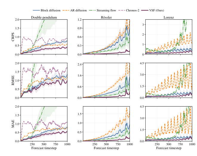
Appendix L Trajectory Forecast Visualizations

We compare sampled forecast trajectories across the evaluated systems and baselines. For the deterministic systems, we additionally show the VSF ensemble predictive mean.

Double pendulum	Image placeholder	Image placeholder	Image placeholder	Image placeholder	Image placeholder
	GT	VSF (Ours)	VSF ensemble	SF	Block diffusion
Double pendulum
Rössler
Lorenz

Figure 15: Qualitative forecasts on the deterministic systems. Columns show ground truth (GT), VSF samples, the VSF ensemble predictive mean, SF, and block diffusion. Sample panels contain

N=10

trajectories; the VSF ensemble is the mean of the samples. The last three rows magnify highlighted regions of the chaotic double-pendulum, Rössler, and Lorenz forecasts.

Sample	GT	VSF (Ours)	SF	Block diffusion	AR diffusion
1
2
3
4
5

Figure 16: Visualization samples from the ground truth and generated trajectories for the partially observed stochastic Lorenz.

$\displaystyle\mathcal{L}_{\mathrm{WM\text{-}VSF}}^{\mathrm{TF}}={}$	$\displaystyle\frac{1}{NM}\sum_{k=0}^{N-1}\sum_{j=1}^{M}\left\\|\widehat{{\bm{u}}}_{s_{k}}^{(j)}-{\bm{u}}_{s_{k}}\right\\|_{2}^{\alpha}$	(F.1)
	$\displaystyle-\frac{1}{2NM^{2}}\sum_{k=0}^{N-1}\sum_{i,j=1}^{M}\left\\|\widehat{{\bm{u}}}_{s_{k}}^{(i)}-\widehat{{\bm{u}}}_{s_{k}}^{(j)}\right\\|_{2}^{\alpha}$
	$\displaystyle+\beta_{\mathrm{KL}}D_{\mathrm{KL}}\!\left(q_{\bm{\phi}}({\bm{z}}\mid{\bm{x}}_{0:N},{\bm{a}}_{0:N-1},{\bm{x}}_{{\bm{s}}},{\bm{s}})\,\\|\,p({\bm{z}})\right),\qquad 0<\alpha<2.$

$\displaystyle\widehat{\operatorname{ED}}_{b}={}$	$\displaystyle\frac{2}{RM}\sum_{r=1}^{R}\sum_{m=1}^{M}\left\\|\mathbf{y}_{b}^{(r)}-\widehat{\mathbf{y}}_{b}^{(m)}\right\\|_{2}$
	$\displaystyle-\frac{1}{R(R-1)}\sum_{\begin{subarray}{c}r,r^{\prime}=1\\ r\neq r^{\prime}\end{subarray}}^{R}\left\\|\mathbf{y}_{b}^{(r)}-\mathbf{y}_{b}^{(r^{\prime})}\right\\|_{2}$
	$\displaystyle-\frac{1}{M(M-1)}\sum_{\begin{subarray}{c}m,m^{\prime}=1\\ m\neq m^{\prime}\end{subarray}}^{M}\left\\|\widehat{\mathbf{y}}_{b}^{(m)}-\widehat{\mathbf{y}}_{b}^{(m^{\prime})}\right\\|_{2},$	(G.9)

Variational Streaming Flow: Probabilistic Forecasting in Physical Time

Abstract

1 Introduction

2 Problem Formulation and Preliminaries

3 Variational Streaming Flow

3.1 Training and Inference

3.2 Variational Training Objective

3.3 Distributional Velocity Reconstruction

4 Experimental Results

4.1 Deterministic Forecasting

4.2 Stochastic Forecasting

4.3 World Model Predictor

5 Conclusion

Limitations and future work.

Acknowledgments

References

Appendix

Appendix A Related Work

Appendix B Motivation for VSF

Proposition B.1 (Fidelity-sensitivity tradeoff).

Proof.

Corollary B.2.

Why introducing a latent model?

Connection to rollout robustness.

This motivates VSF.

Appendix C A variational objective for clean streaming trajectories

Proposition C.1 (Conditional-velocity evidence lower bound).

Proof.

Equivalent local conditioning.

Appendix D Population Energy Reconstruction and Energy-Distance Control

Proposition D.1 (Prior-predictive energy-distance control).

Proof.

Interpretation of aggregate alignment.

Appendix E Training and inference details

E.1 Forecasting training and inference

Appendix F World-model VSF predictor: training and inference

Appendix G Evaluation metrics

G.1 Deterministic ground truth

Continuous ranked probability score (CRPS).

Root mean squared error (RMSE) and mean absolute error (MAE).

G.2 Stochastic ground truth

Conditional mean error (CME) and conditional standard-deviation error (CSE).

First-order Wasserstein distance (W1W_{1}).

Energy distance (ED).

Appendix H Dataset Statistics

H.1 Deterministic Datasets

Double pendulum.

Rössler system.

Lorenz system.

H.2 Stochastic Datasets

Stochastic data-generation.

Stochastic Rössler system.

Stochastic Lorenz system.

H.3 World-Model Datasets

PushT.

Cube.

TwoRoom.

Reacher.

Appendix I Experimental Setup

I.1 Forecasting

Baseline models.

Method-specific settings.

Chronos-2 calibration.

Experimental details.

I.2 World Models

Baseline models.

Method-specific settings.

Experimental details.

Appendix J Full ablation results

Energy-score exponent α\alpha and MSE.

KL regularization.

Latent contribution.

Latent resampling.

Latent-source and prior-alignment variants.

Does latent conditioning help?

Does variational training help?

Why prior alignment matters.

Appendix K Rollout Error Plots

Appendix L Trajectory Forecast Visualizations

Appendix M World-Model Latent-Trajectory Visualizations

First-order Wasserstein distance ( $W_{1}$ ).

Energy-score exponent $\alpha$ and MSE.