Testing Procedures for Strict Pleiotropy in Genetic Association Studies
Abstract
Pleiotropy, the phenomenon in which a single genetic variant influences multiple traits, is a fundamental feature of genome biology and an important consideration in statistical genetics. Many statistical methods exist that leverage pleiotropy to increase the power of association tests, but they are often designed to identify SNPs which are associated with at least one of the underlying traits. Only a limited number of methods exist for identification of “strict pleiotropy”, i.e. those associated with more than one trait, but these methods are either restricted to a small number of traits or become computationally challenging as the number of traits increases. In this paper, we develop two testing procedures to identify SNPs under strict pleiotropy and determine the corresponding minimum number of associated traits. Both methods rely only on z-scores available from genome-wide association studies (GWAS) and are applicable to independent as well as correlated traits. The first procedure is frequentist in nature and is designed to control the family-wise-error rate. The second procedure is based on the local false discovery rate and provides improved power while maintaining FDR control. We conduct extensive simulation studies to compare the performance of the proposed methods with alternative methods for testing strict pleiotropy. Finally, we demonstrate an application of the proposed methods to Alzheimer’s disease-related biomarkers for the goal of distinguishing SNPs that may represent biomarker-specific variations from those that are related to disease-relevant biology.
1Department of Oncology, Johns Hopkins University, School of Medicine, Baltimore, MD
2Department of Biostatistics, Johns Hopkins Bloomberg School of Public Health, Baltimore, MD
Keywords: Genome-wide association study (GWAS), pleiotropy, local false discovery rate, composite hypothesis, family-wise error rate, variance component model, single-nucleotide polymorphism (SNP)
1 Introduction
Pleiotropy, the phenomenon where a single genetic variant influences multiple traits [32, 33], is a fundamental property of genome biology and a key concept in statistical genetics. Genome-wide association studies (GWAS) have provided evidence of widespread pleiotropy across a broad range of human traits [2, 25, 26, 36, 38], demonstrating that genetic architecture is highly interconnected. Researchers have leveraged pleiotropy to improve the power of SNP discovery in GWAS. Assuming that the traits are associated through pleiotropy, multivariate and multi-trait GWAS methods have been developed to jointly test associations between genetic variants and multiple related phenotypes, thereby improving power to detect SNPs associated with the traits [41, 42, 3, 13, 4, 27]. However, these approaches primarily test whether a SNP is associated with at least one trait within a phenotype set, rather than explicitly testing for multi-trait per se.
Several methods [44, 28, 29, 24] have been developed to test for “strict” multi-trait association under suitable composite null hypotheses. However, these methods are difficult to generalize beyond two traits and fail to account for genetic correlations among traits and for correlations induced by GWAS sample overlap. [31] introduced a sequential testing framework for pleiotropy across more than two traits, though their method requires individual-level data, which limits its applicability, as in practice, we may not have access to individual-level data. In addition to traditional multivariate testing frameworks, empirical Bayes approaches based on the local false discovery rate (lfdr) [7, 8, 35] have become useful tools for testing genetic effects across multiple traits. Recently, Sun et al. [34] proposed the conditionally symmetric multidimensional Gaussian mixture model (csmGmm) for testing strict pleiotropic association while controlling the false discovery rate (FDR), but this method faces substantial computational challenges when the number of traits is large.
Testing for strict pleiotropy becomes highly relevant when investigating the genetic association of latent health conditions that manifest through multiple biomarkers. For example, the early stage of Alzheimer’s disease (AD), when cognitive symptoms are not yet developed, is characterized by alterations in multiple biomarkers, including amyloid beta, phosphorylated tau (p-tau), neurogranin, synaptosomal-associated protein 25 (SNAP-25), and neurofilament light (NFL) [11, 12]. Likewise, inflammation underlies various complex diseases, including cardiovascular, autoimmune disorders, and metabolic disorders, and is commonly assessed using biomarkers such as C-Reactive Protein (CRP), high-sensitivity CRP, Erythrocyte Sedimentation Rate (ESR), immunoglobulin E (IgE), and tumor necrosis factor (TNF) [23, 30]. In such cases, genetic variants associated with individual biomarkers may simply reflect biomarker-specific biological processes. But variants that co-regulate multiple biomarkers simultaneously are more likely to provide insight into the biological mechanisms of underlying latent conditions. Further, identifying such pleiotropic variants can also lead to a proper genetic “instrument” for testing for causal effects of latent exposures like inflammation on health conditions [17]. When the number of biomarkers is relatively large, it may be, however, too restrictive to identify SNPs which are associated with all traits, and a more suitable formulation for the alternative hypothesis would be to identify SNPs which show a certain “degree” of pleiotropy, i.e. they are associated with a minimum number, say, , of the traits
In this study, we revisit the methodology for testing for strict pleiotropy and make several novel contributions. We propose two testing methodologies to identify pleiotropic SNPs by using the z-scores readily available from GWAS studies. The first method uses a minimum of z-scores to test the alternative that a SNP affects all traits, and we demonstrate that this simplified test statistic is asymptotically equivalent to the likelihood-ratio test requiring individual-level data. For the general alternative that a SNP affects at least of traits, we develop a sequential test based on z-score quantiles while controlling the family-wise error rate (FWER). The advantages of the test are that it is simple, it does not involve any complex estimation method, and hence it is computationally efficient to implement, even when the number of traits is large. Moreover, its performance is robust to the dependence structure among the traits.
Within the same framework, we further propose a FDR control method for testing the pleiotropy architecture across SNPs. The test accounts for the correlation among observed traits arising from overlapping samples, as well as the correlation of SNP effects across traits due to genetic correlation. While csmGmm models the mean structure of z-scores, our method models the variability of z-scores across SNPs by introducing fewer parameters to reduce computational burden for a large number of biomarkers. We also provide a step-by-step estimation procedure that facilitates the implementation of the proposed test and improves computational efficiency. We conduct extensive simulation studies to compare the performance of these novel methods with that of existing methods. We illustrate the application of these two methods through pleiotropic analysis of established Alzheimer’s disease biomarkers using GWAS summary statistics.
2 Statistical Framework and Methods
Consider traits and suppose the objective is to identify SNPs that influence all or a subset or none of these traits simultaneously. For each trait , let denote the observed values of the trait across individuals. Suppose is the vector of genetic variant for all in the dataset for biomarker. It is important to note that the datasets corresponding to different traits may partially or completely overlap in individuals.
In GWAS, a quantitative trait is typically modeled using a linear regression by assuming
| (1) |
where represents the effect size (slope) of genetic variant. The vector includes other covariates, such as age, sex, and genetic principal components, and is a vector of random errors. When the trait of interest is binary (e.g., disease status), a logistic regression model is used instead.
The estimated slope , its standard error and the Wald test statistic (or z-score ) are publicly available from GWAS summary statistic. Our two sequential testing procedures use these Wald statistics as their primary inputs.
2.1 Formulation of the hypothesis
Consider the hypothesis where the goal is to detect variants that affect at least out of traits. The test is formulated as:
| (2) |
Under , the SNP influence atmost traits, i.e., no group of or more traits simultaneously show nonzero effects. Equivalently, the alternative hypothesis asserts that there exists a subset of at least traits for which the variant has a nonzero effect.
2.2 The minimum-test and a connection with likelihood-ratio
We first test whether a SNP affects all traits simultaneously to assess “strict pleiotropy”. We propose a simple test using the Wald statistic, which is readily available, and show that the test is asymptotically equivalent to the likelihood ratio test, which requires individual-level data.
First, we fix a variant and discuss the methodology to test the hypothesis (2) for , where the alternative asserts that the variant influences all traits. We begin by considering the individual hypotheses for each trait as
| (3) |
The rejection of hypothesis depends on how large the statistic is. The global null hypothesis , and . We reject the global null only if all individual nulls are rejected, i.e., all the statistics exceed the corresponding threshold. Therefore, an intuitive and simple test statistic for assessing pleiotropy as the minimum absolute Wald statistic across all traits:
| (4) |
where . There is no simple form of the asymptotic distribution of the test statistic, particularly under dependence. By applying the intersection-union test (6) we obtain the rejection region for a significance level , as stated in the following proposition.
Proposition 1.
For , let , where denotes the cumulative distribution function of the standard normal distribution. Then where and denotes the parameter space under .
The rejection region of each corresponding to is also . Therefore, will be rejected if all the individual fall in . To perform the above test, we do not need access to individual-level data; we only need the estimated effect size and its standard error, which are available from the GWAS summary statistics. Also, the above test is not affected by correlation among the GWAS data sets.
Next we consider the likelihood-ratio test for the composite null hypothesis , assuming individual-level data are available from individuals and the traits follow a multivariate Gaussian distribution. Also assume is the full design matrix combining all covariates, and is the reduced design matrix obtained by removing the column corresponding to the genetic variant. Then the following proposition presents the test statistic and the corresponding rejection region to perform the hypothesis test (see derivation in Sec
Proposition 2.
The likelihood ratio test is given by
| (5) |
where and are the projection matrices onto the column spaces of and , respectively, , with being the identity matrix, and denotes the diagonal element of .
Also, for level , , where is the vector of all the parameters needed to specify the full model for , and with being the cumulative distribution function of the distribution.
See the Supplements for the derivation of the test statistics and the proof of the asymptotic distribution.
Remark 1.
The representation of the LRT in the above form suggests the optimality of minimum-test-statistics for testing the composite null hypothesis of interest. In particular, for any individual hypothesis , we know that the Wald statistic is asymptotically equivalent to the LRT. In the current setting, since the global null hypothesis is , the minimum of the individual Wald statistics lies in the rejection region if and only if each individual Wald statistic falls in its respective rejection region. Equivalently, the individual LRT statistics for testing fall in the rejection region for all . Therefore, has an asymptotically equivalent rejection region to the likelihood ratio test for assessing versus .
2.3 A Sequential Quantile-based Test (SQT)
Given the optimality property of the min-test for testing against , in this section, we will consider a quantile-based test for testing when . Further, we note that in GWAS, typically, Bonferroni correction is applied for the number of SNPs tested to maintain FWER. Here, . In other words, the test for each SNPs is performed at a fixed threshold , where denotes the total number of SNPs. However, in the context of testing pleiotropic effects for SNPs across multiple traits, the use of a fixed threshold across SNPs is not efficient, and we propose a sequential version of the test that can adaptively adjust the significance threshold level at each stage depending on the number of SNPs that passed the previous stage. The algorithm is described step-by-step below.
Step 1: Extract the -values of the common variants from the GWAS studies after harmonization and create a matrix , where is the number of common variants. Also retain the variant ID corresponding to each row of the matrix.
Step 2: For each SNP , sort the -values in ascending order and denote them by
Step 3: Start with and . We apply the following iterative procedure, which adaptively filters variants using multiple-testing-adjusted thresholds:
- i.
For , let denote the number of SNPs remaining in and calculate
- ii.
Retain the SNPs satisfying
and update by keeping only these SNPs. Record the corresponding SNP IDs as variants identified as being associated with at least traits.
While running the procedure, if no SNPs survive at iteration , this indicates that there are no SNPs associated with more than biomarkers. Furthermore, if the goal is to identify variants influencing at least biomarkers, the above algorithm is applied sequentially from through . The quantity in controls the type one error for each variant to test , while the quantity maintains the FWER at for testing across many variants selected in the previous step, which leads to the following proposition.
Proposition 3.
For SQT with nominal level , the FWER is maintained at at each iteration corresponding to hypothesis asymptotically.
3 Empirical-Bayes method and FDR control
Thus far, we have developed a testing procedure that controls the FWER. In this section, we present an alternative approach for testing (2) that controls the FDR rather than the FWER, with the aim of improving statistical power. The proposed method models the z-scores using a mixture of symmetric Gaussian distributions.
We have , if there is no true effect of SNP on trait , i.e., . Otherwise, the score increases with sample size, as it is computed without centering. So we assume that the score follows for some large variance if , and the marginal distribution can be written as
| (6) |
with , where corresponds to the probability of a randomly selected SNP being associated with trait . Define as the vector of indicator variables that indicate whether the SNP is associated with the -th trait across and , denoting the number of corresponding non-zero effects. Further, we observe that z-scores across a pair of biomarkers can be correlated due to the correlation () in true effect sizes for the SNPs across the biomarkers and due to the correlation in estimation error () that arises when there is sample overlap in the underlying GWAS. In the appendix, we show that under the proposed modeling framework, one can express for any SNP that is associated with none or only one of the traits, and for any SNP that is associated with both traits. Now, if we denote as the vector of observed z-scores associated with the -th SNP, then the local false discovery rate under the composite null hypothesis can be written as
| (7) |
where denotes the probability of the configuration and denotes the -variate normal density under mean zero and variance-covariance matrix , which depends on the configuration , evaluated at . Evaluation of lfdr in the above setting requires first the estimation of the unknown parameters , i.e the probability distribution of , and the underlying variance-covariance parameters indexed by , and , . We optimize using the EM algorithm, accounting for the mixture-likelihood structure induced by the latent factors . The performance of the test depends on . For instance, suppose , where corresponds to a larger subset of traits being associated with a SNP than . In this case, even when the evidence for association for an individual SNP corresponding to the configuration to be higher than , i.e. , one may have . Therefore, to avoid parameter estimates that correspond to substantially higher probabilities for configurations in with more non-zero values than with fewer non-zero values, we propose optimizing the penalized complete log-likelihood of the following form using the standard EM algorithm-
| (8) |
where is 1 if , otherwise 0, the sum inside the penalty term corresponds to all pairs of and that differ in their value for only one biomarker, with denoting the configuration with more associated biomarkers, and the ratio corresponding to the odds of a SNP being associated with the biomarker given that the other configurations of association are fixed. For example, if there are three biomarkers, the penalty term is given by . The parameter softly puts restriction such that is not larger than .
It is important to choose in a data-driven manner. For a given SNP, let . If corresponds to a rare event, then it might happen that involving more associated traits than and . Therefore, multiplication by the configuration probabilities can suppress the contribution of in the mixture distribution and hence favor the configuration . We refer to SNPs for which this occurs as discrepant SNPs. For such SNPs, this discrepancy can lead to a relatively small estimated mixture likelihood. For , we therefore aggregate the log-mixture density of the discrepant SNPs, as given by
where denotes the set of discrepant SNPs. The goal of penalization is to improve the mixture fit for these SNPs while avoiding substantial deterioration in the overall fit of the model. For the SNPs that do not affect any trait, their mixture densities are expected to change little under penalization. Hence, we apply VGM-lfdr and retain the set of SNPs identified as affecting at least one trait. Let denote the sum of their log-mixture density. For each candidate value of , we compute using the same set and also record using the SNPs in . We then quantify the improvement among discrepant SNPs with the corresponding loss in overall mixture fit through
and choose the value of that maximizes this ratio. A simulation study in the Appendix evaluates the performance of lfdr-VGM with this automated choice of and illustrates how discrepant SNPs can arise in the absence of penalization.
Remark 2.
In csmGmm, for each trait , the score is modeled using a Gaussian mixture, similar to our approach. However, to capture nonzero effect sizes, the method uses pairs of shifted Gaussian components, and , where for , with . Moreover, the mean parameters used to represent nonzero SNP effects may depend on the particular configuration of the vector . While this construction provides a flexible way to model non-null effects, it also has some practical limitations. In genome-wide applications, significant z-scores can be quite scattered. As a result, even a large z-score may have very small local density under a component such as , unless the observed value lies sufficiently close to the chosen mean . Using multiple mean parameters can help address this issue by covering a wider range of possible effect sizes. However, this introduces another practical question: how should the number of mean parameters be chosen? Increasing the number of components also increases the complexity of the model, which can make the computation challenging when the number of traits is large. A simple way to reduce this difficulty is to truncate the z-scores and then use only a small number of mean parameters. This is the approach we adopt in both the empirical study and the real data analysis. However, changing the threshold can impact the power and FDR of the method.
Here, we take a more robust approach to modeling the z-scores. We assume the scores follow across all configurations if the corresponding effect size is non-zero. Considering a single parameter captures the variability of large z-scores, thereby circumventing issues arising from near-zero density, and also keeps the number of parameters minimal.
4 Simulation
In this section, we present simulation studies to evaluate the performance of our two proposed sequential tests and compare them with other existing methodologies: PLACO Plus and csmGmm. PLACO [29] is a statistical method developed to detect “strict” pleiotropic SNPs in the setting of two traits. For a given SNP, the PLACO test statistic is defined as the product of the corresponding -scores from the two studies, and its null distribution is derived under the assumption that the two -scores are independent. Later, PLACO Plus [24] was introduced to accommodate dependence between the -scores across the two traits. However, extending this framework to more than two traits is challenging because of the increasing complexity involved in deriving the asymptotic null distribution of the product statistic. We first consider two traits so that the performance of the proposed method can be compared against both PLCO and csmGMM. We further evaluate the performance of the proposed lfdr method against cmGmm for =5 biomarkers. The general structure of the simulation for any number of traits is as follows:
- 1.
The genotype status for each SNP is generated from a trinomial distribution in Hardy-Weinberg equilibrium, with a fixed minor allele frequency of 0.25.
- 2.
Configuration selection for each SNP : We set the total number of SNPs to , with 99% of SNPs assumed to have no effect on any of the traits. For each of the remaining “non-null” SNPs, we sample a configuration of using a specified probability distribution and correspondingly allow it to be associated with a given subset of the traits. We choose proportional to so that configurations of a SNP being associated with more traits are less likely than being associated with fewer traits, but it also corresponds to ”positive” dependence for SNPs simultaneously being associated with multiple traits. For example, when , we selected with .
- 3.
Trait assignment: The non-zero effect sizes are generated from , where .
- 4.
z-score computation: For the -th individual and the -th SNP, the -dimensional trait vector is generated from a multivariate normal distribution with mean , where denotes the SNP value, and a covariance matrix which corresponds to a residual variance of the biomarkers of 0.1 and a correlation value of 0.3. After generating the data, for each SNP , we perform a linear regression of on and compute the corresponding -scores.
Figure 1 summarizes the performance of alternative methods for when and . Overall, both proposed tests, SQT and lfdr-VGM with , maintain the corresponding error criteria, i.e., FWER for the former and FDR for the latter, at the desired level. Under the composite null hypothesis, a false positive is considered any SNP that is not associated with both traits but is declared significant. We observe that PLACO, which is designed to maintain a type-I error averaged over the different sub-null hypotheses with weights according to estimates of the proportions of SNPs in different components, can have substantially inflated FWER because it does not guarantee suitable error control under each sub-null hypothesis. In particular, in GWAS, the number of SNPs associated with neither trait is typically much larger than those associated with only one trait; as a result, the average type-I error is dominated by SNPs that are under the global hypothesis. Thus, the FWER for PLACO can be particularly large, as the likelihood of a single false positive result from SNPs that are associated with one trait but not the other is very high. The csmGmm method, by contrast, controls FDR, but it appears more conservative than lfdr-VGM. In terms of power, PLACO was the most powerful of the three methods, which is not surprising given that the method does not provide strict FWER or FDR control. Between lfdr-VGM and csmGmm, lfdr-VGM exhibited higher power across the simulation settings. This is consistent with csmGmm’s conservative FDR, which remained substantially below the nominal level and consequently yielded fewer discoveries in our settings.
Next, we considered the setting of biomarkers. From Figure 2, we observe that both methods, SQT and lfdr-VGM, maintain the respective error criteria, i.e., FWER and FDR, under each type of null hypothesis, , . We observe that the power of both methods decreases as increases, and both have the lowest power when , i.e., for detecting SNPs associated with all five traits. For the testing of , where we could apply csmGmm, we again observe that the power of the lfdr-VGM method was consistently higher than csmGMM across different scenarios (see Figure 3). We present results from additional simulation studies in the Supplemental Materials to investigate the sensitivity of the lfdr-VGM method to the choice of the tuning parameter “”. We find that across , , and , the method maintains FDR and has comparable power. Additional simulation results for different sample sizes are also presented in Supplemental Materials.
Observe that csmGmm has an FDR that is substantially lower than the nominal level. We truncate the z-scores, as they are quite scattered, and then model them using a one-mean parameter (both positive and negative numbers of the same magnitude) for each trait. We observe that, for some SNPs identified as pleiotropic by lfdr-VGM, one of the z-scores is large and the other one is not sufficiently large, such that the smaller pair is not close enough to the estimated mean induced by the alternative and therefore yields almost zero probability under the alternative and consequently is not identified as pleiotropic by csmGmm. Also, csmGmm imposes a constraint on the mean parameters: the mean parameters of the -scores under the configuration where a SNP affects exactly traits must be larger than those under configurations where the SNP affects fewer traits. Hence, in our setting, if one wants to allow a smaller second mean parameter under the two-trait alternative, this parameter must still be larger than the corresponding mean parameters under the single-trait alternatives. Although this constraint is maintained in csmGmm, it can create difficulties when one component of the -score is large while the other is close to zero. In such cases, the joint density under all configurations may happen to be almost 0, leading to numerical issues.
.
.
| RSID | CHR | POS | Nearest gene | A -value | ptau -value | PLACO | SQT | csmGmm | lfdr-VGM |
|---|---|---|---|---|---|---|---|---|---|
| rs769449 | 19 | 44906745 | APOE | 1.69e-321 | 9.59e-95 | 0 | Identified | 9.20e-14 | 0 |
| rs117583674 | 7 | 37040693 | ELMO1 | 1.72e-07 | 0.007832 | 2.63e-06 | No | 0.5831 | 0.0334 |
| rs6733839 | 2 | 127135234 | BIN1 | 1.65e-06 | 1.26e-05 | 9.07e-09 | No | 0.2417 | 0.005 |
| rs34113929 | 3 | 190902357 | GMNC | 0.019 | 2.70e-28 | 1.74e-10 | No | 0.7062 | 0.99 |
| rs4844610 | 1 | 207629207 | CR1 | 1.84e-09 | 0.003016 | 1.10e-07 | No | 0.3921 | 0.0008 |
| rs9430717 | 1 | 9710947 | PIK3CD | 1.12e-07 | 0.1503 | 0.000454 | No | 0.8581 | 0.0266 |
| Probability | Abeta | ptau | NFL | Snap25 | Neurogranin |
|---|---|---|---|---|---|
| 0 | 0 | 0 | 0 | 0 | |
| 0 | 0 | 1 | 0 | 0 | |
| 0 | 0 | 0 | 1 | 1 | |
| 0 | 0 | 0 | 0 | 1 | |
| 0 | 0 | 0 | 1 | 0 | |
| 1 | 1 | 1 | 1 | 0 | |
| 0 | 1 | 0 | 0 | 0 | |
| 0 | 1 | 1 | 0 | 0 | |
| 1 | 1 | 0 | 1 | 0 | |
| 1 | 0 | 1 | 1 | 0 | |
| 0 | 1 | 1 | 1 | 0 | |
| 1 | 1 | 1 | 0 | 0 | |
| 1 | 0 | 0 | 1 | 0 | |
| 0 | 1 | 0 | 1 | 0 | |
| 0 | 0 | 1 | 1 | 0 | |
| 1 | 1 | 0 | 0 | 0 | |
| 1 | 0 | 0 | 0 | 0 | |
| 0 | 0 | 1 | 0 | 1 | |
| 1 | 0 | 1 | 0 | 0 | |
| 0 | 1 | 0 | 0 | 1 | |
| 0 | 0 | 1 | 1 | 1 | |
| 1 | 0 | 0 | 0 | 1 | |
| 0 | 1 | 0 | 1 | 1 | |
| 0 | 1 | 1 | 0 | 1 | |
| 1 | 0 | 0 | 1 | 1 | |
| 1 | 0 | 1 | 0 | 1 | |
| 1 | 1 | 0 | 0 | 1 | |
| 0 | 1 | 1 | 1 | 1 | |
| 1 | 0 | 1 | 1 | 1 | |
| 1 | 1 | 0 | 1 | 1 | |
| 1 | 1 | 1 | 0 | 1 | |
| 1 | 1 | 1 | 1 | 1 |
| Amyloid- | p-tau | NfL | SNAP-25 | Neurogranin | |
|---|---|---|---|---|---|
| Amyloid- | 1.0000 | -0.2500 | 0.0004 | 0.0004 | 0.0013 |
| p-tau | -0.9331 | 1.0000 | 0.0015 | -0.0011 | -0.0007 |
| NfL | -0.1030 | 0.0034 | 1.0000 | -0.0772 | -0.0130 |
| SNAP-25 | 0.1071 | -0.0716 | -0.3803 | 1.0000 | 0.6193 |
| Neurogranin | 0.0588 | 0.0768 | 0.2585 | 0.5971 | 1.0000 |
| rsid | chr | pos | Nearest gene | A | p-tau | NFL | SNAP-25 | Neurogranin | # traits lfdr-VGM | # traits SQT |
| rs429358 | 19 | 44908684 | APOE | 3.39e-38 | 9.75e-16 | 0.00323 | 3.13e-176 0 | .433 | 4 | 4 |
| rs2972558 | 19 | 44852884 | NECTIN2 | 9.28e-17 | 0.01005 | 0.000638 | 6.13e-41 | 0.574 | 4 | 3 |
| rs73045691 | 19 | 44937272 | APOC4 | 5.60e-07 | 0.001608 | 0.000337 | 9.91e-20 | 0.134 | 4 | 3 (LD with rs77301115) |
| rs8103315 | 19 | 44750911 | BCL3 | 7.29e-14 | 2.07e-05 | 3.67e-02 | 1.92e-30 | 7.72e-01 | 3 | 3 |
| rs157585 | 19 | 44894255 | TOMM40 | 1.35e-44 | 1.10e-14 | 0.405 | 2.07e-46 | 0.956 | 3 | 3 |
| rs28795074 | 19 | 44933400 | APOC1P1 | 6.54e-07 | 0.004795 | 0.153 | 1.37e-06 | 0.507 | 3 | 0 |
| rs62117205 | 19 | 44752009 | BCL3 | 9.48e-09 | 3.391 6.975e-4 | 0.964 | 1.29e-10 | 0.922 | 3 | 2 |
| rs2070116 | 22 | 42210251 | OGFRP1 | 1.13e-01 | 9.01e-01 | 4.13e-02 | 4.51e-09 | 1.57e-02 | 2 | 1 |
| rs4803759 | 19 | 44824202 | BCAM | 2.51e-11 | 1.02e-01 | 3.75e-01 | 8.20e-25 | 3.02e-01 | 2 | 2 |
| rs4803824 | 19 | 45448020 | ERCC1 | 9.18e-01 | 5.13e-01 | 6.92e-01 | 2.41e-08 | 4.66e-04 | 2 | 0 |
| rs1671152 | 19 | 55014977 | GP6-AS1 | 3.74e-01 | 7.51e-01 | 7.01e-01 | 4.55e-07 | 1.09e-13 | 2 | 2 |
| rs7210399 | 17 | 29453198 | TAOK1 | 1.76e-01 | 5.96e-02 | 8.06e-01 | 1.96e-06 | 8.24e-09 | 2 | 2 (LD with rs1967556) |
| rs1298104 | 16 | 4386444 | TFAP4 | 4.00e-01 | 6.42e-02 | 9.06e-01 | 1.34e-08 | 1.21e-02 | 2 | 0 |
| rs6580981 | 12 | 54329244 | COPZ1 | 7.43e-01 | 4.93e-01 | 6.54e-01 | 2.71e-03 | 1.25e-07 | 2 | 0 |
| rs10822145 | 10 | 63174788 | JMJD1C | 9.95e-01 | 1.72e-01 | 1.19e-01 | 5.47e-17 | 3.85e-13 | 2 | 2 (LD with rs7896518) |
| rs113422568 | 10 | 102578181 | SUFU | 4.77e-01 | 3.49e-01 | 6.59e-02 | 1.82e-04 | 5.54e-06 | 2 | 0 |
| rs61469632 | 9 | 132986603 | GFI1B | 8.95e-01 | 9.53e-02 | 2.28e-01 | 1.69e-11 | 1.74e-03 | 2 | 1 |
| rs467369 | 9 | 134040643 | BRD3 | 7.28e-01 | 5.53e-01 | 7.06e-01 | 4.39e-07 | 6.68e-03 | 2 | 0 |
| rs4734879 | 8 | 105570896 | ZFPM2 | 1.89e-02 | 6.66e-01 | 7.77e-01 | 4.42e-09 | 6.14e-13 | 2 | 2 |
| rs193117411 | 7 | 106685425 | CCDC71L | 4.73e-01 | 5.96e-01 | 6.50e-01 | 1.14e-08 | 2.78e-02 | 2 | 0 |
| rs342296 | 7 | 106732457 | LINC02577 | 6.20e-03 | 5.46e-01 | 1.53e-01 | 2.57e-172 | 1.79e-12 | 2 | 2 |
| rs9389269 | 6 | 135106021 | HBS1L | 6.39e-01 | 7.78e-02 | 3.67e-01 | 2.28e-05 | 3.68e-09 | 2 | 1 |
| rs115318824 | 5 | 89001177 | MEF2C-AS1 | 1.41e-01 | 4.07e-01 | 4.49e-01 | 1.49e-05 | 5.58e-03 | 2 | 0 |
| rs10900809 | 5 | 132490630 | IRF1 | 1.27e-01 | 6.36e-01 | 5.88e-01 | 5.67e-06 | 4.11e-10 | 2 | 2 |
| rs1354034 | 3 | 56815721 | ARHGEF3 | 5.25e-01 | 3.53e-01 | 1.93e-01 | 2.23e-06 | 5.24e-14 | 2 | 2 |
| rs1501600 | 3 | 190903230 | GMNC | 2.32e-02 | 8.43e-29 | 2.91e-03 | 9.53e-03 | 1.01e-01 | 2 | 1 |
| rs6733839 | 2 | 127135234 | BIN1 | 1.65e-06 | 1.26e-05 | 2.61e-01 | 6.01e-01 | 9.22e-01 | 2 | 0 |
| rs750439 | 1 | 156460957 | MIR9-1HG | 7.49e-01 | 7.36e-01 | 4.08e-01 | 5.55e-11 | 5.67e-03 | 2 | 1 |
| rs4844610 | 1 | 207629207 | CR1 | 1.84e-09 | 3.02e-03 | 3.20e-01 | 6.37e-01 | 7.99e-01 | 2 | 1 |
5 Data Example
We apply SQT and lfdr-VGM to GWAS summary statistics for biomarkers related to Alzheimer’s disease (AD), with PLACO Plus and csmGmm included for comparison when applicable. Cerebrospinal fluid (CSF) amyloid- (A42) and phosphorylated tau (p-tau) reflect key pathological changes in AD: A42 decreases in CSF as amyloid aggregates in the brain, whereas p-tau increases with neuronal injury (see [14, 15]). GWAS summary statistics for A42 and p-tau were obtained from the European Alzheimer & Dementia Biobank, comprising 31 cohorts and 13,116 individuals, including 8,074 in the discovery sample [16].
We first consider the two-biomarker analysis and apply PLACO Plus, SQT, lfdr-VGM, and csmGmm to identify variants associated with both A42 and p-tau. PLACO Plus is applied at the genome-wide threshold , SQT controls genome-wide FWER at 0.05, and lfdr-VGM and csmGmm are applied at FDR 0.05. The data-driven procedure selects for lfdr-VGM, yielding estimated probabilities 0.999, , , and for configurations , , , and , respectively. The estimated correlations are and , indicating correlation arising from sample overlap and strong correlation between nonzero effects across the two biomarkers. For all methods, we apply clumping and thresholding using and a 500 kb window to retain independent lead SNPs.
Table 1 reports independent lead SNPs identified by at least one method. All four methods identify the chromosome 19 APOE region as showing pleiotropic association with both biomarkers. PLACO Plus and lfdr-VGM also identify additional loci, although their findings differ. Both identify a chromosome 2 locus near BIN1. PLACO Plus additionally identifies a chromosome 3 locus for which the index SNP is strongly associated with p-tau () but only modestly associated with A (). In contrast, lfdr-VGM identifies one locus on chromosome 7 and two on chromosome 1 that are not genome-wide significant under PLACO Plus. The estimated probability of the SNP affecting A is substantially smaller than the probability of a SNP affecting both traits, leading lfdr-VGM to identify rs9430717.
We next extend the analysis to five AD-related biomarkers by including neurogranin, neurofilament light (NFL), and SNAP-25. CSF neurogranin is elevated in AD-related dementia and MCI due to AD [19, 39, 20]; NFL, a marker of axonal injury, is increased in CSF and plasma [9, 22, 40]; and CSF SNAP-25 fragments are elevated even at early stages of AD [5, 43]. NFL GWAS summary statistics were obtained from 11 European cohorts in the Rotterdam and Rhineland Studies, comprising 18,532 individuals [1]. SNAP-25 and neurogranin GWAS data were obtained from the UK Biobank, with the SNAP-25 discovery sample including 47,745 individuals of European ancestry [21].
We apply SQT and lfdr-VGM to identify SNPs and the minimum number of biomarkers with which they are associated. The data-driven procedure selects for lfdr-VGM. Table 2 reports the estimated latent configuration probabilities. As expected, the null configuration has the largest probability, approximately 0.997. Notably, the configuration corresponding to joint effects on A, p-tau, NFL, and SNAP-25 has a relatively high estimated probability, exceeding those of a subset of at least two traits. The SNAP-25–neurogranin configuration also has a comparatively high probability, whereas configurations in which neurogranin is jointly affected with other biomarkers are much less common. These patterns indicate stronger estimated shared genetic association for A, p-tau, NFL, and SNAP-25, and between SNAP-25 and neurogranin.
Table 3 reports the estimated correlations between random errors in the upper triangle and between nonzero effect sizes in the lower triangle. As expected from overlapping GWAS samples, the random errors are correlated for A and p-tau and for SNAP-25 and neurogranin. The estimated nonzero effects are also strongly correlated between A and p-tau and between neurogranin and SNAP-25.
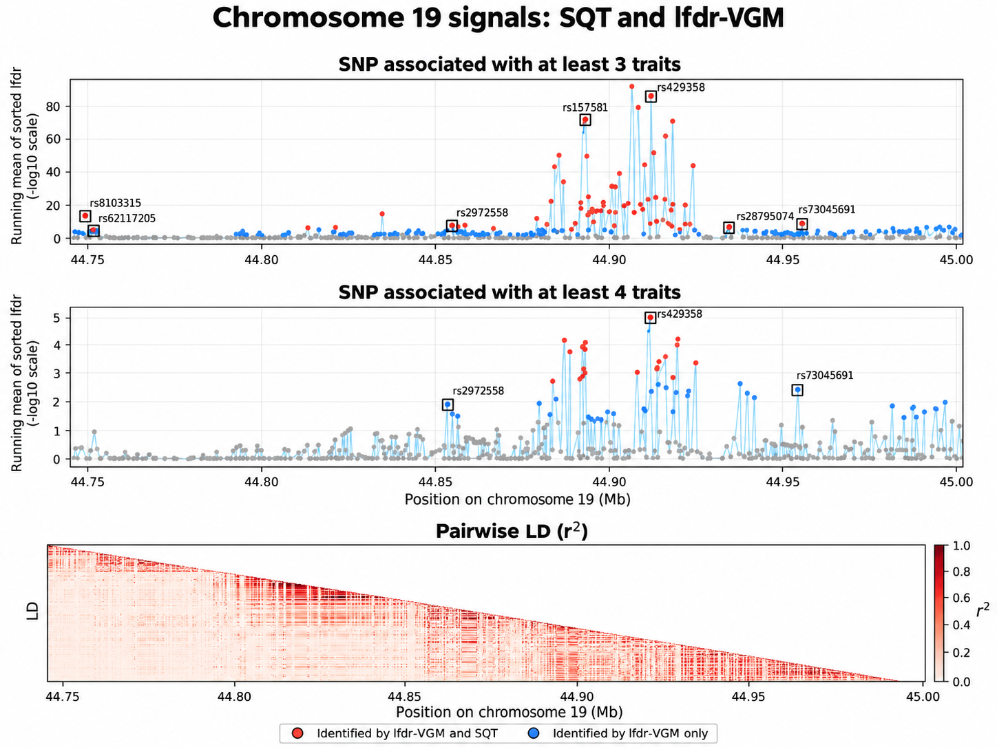
Figure 3 compares SQT and lfdr-VGM in the APOE region. lfdr-VGM identifies more SNPs as affecting at least three and at least four traits. The additional discoveries at the four-trait level are partly explained by the relatively large estimated probability of configuration , corresponding to joint effects on A, p-tau, NFL, and SNAP-25, compared with its size-three subsets. Table 4 reports the independent SNPs identified after clumping and thresholding. The APOE-region findings are consistent with previous reports linking rs7412 and rs429358 to Alzheimer’s disease (see [18, 37, 10]). Both SQT and lfdr-VGM identify rs429358 as affecting at least four traits and rs7412 as affecting at least three. lfdr-VGM additionally identifies rs2972558, which is in LD with rs7412, as affecting at least four traits. Overall, SQT identifies SNPs on chromosomes 3, 5, 7, 8, 10, 17, and 19 as affecting at least two traits, whereas lfdr-VGM identifies independent SNPs across chromosomes 1, 2, 3, 5, 6, 7, 8, 9, 10, 12, 16, 17, 19, and 22.
6 Discussion
In this article, we proposed two methods, SQT and lfdr-VGM, for identifying pleiotropic SNPs using Wald test statistics. A key novelty of both methods is that, beyond detecting pleiotropy, they can determine the minimum number of traits a SNP is associated with at a given significance level. SQT has several practical advantages. It is simple and computationally efficient to implement, accommodates both independent and correlated traits, can be applied to an arbitrary number of traits, unlike methods such as PLACO that are restricted to a smaller number of traits, and requires only summary-level test statistics rather than individual-level data. The lfdr-VGM approach involves estimation of the underlying mixture model and is therefore computationally more involved than SQT. However, it provides a substantial power gain. While SQT controls FWER, lfdr-VGM controls FDR, allowing it to identify more pleiotropic variants while maintaining appropriate error control. In addition, lfdr-VGM explicitly models both the correlation among random errors across traits, which can arise from sample overlap, and the correlation among nonzero genetic effects. Incorporating these dependence structures into the joint distribution of the Wald statistics further improves its ability to detect pleiotropic signals.
The performance of csmGmm depends on the number of nonzero mean parameters used and has power comparable to SQT in our current setting. It is also conservative in controlling the FDR at the nominal level (one mean parameter is used for each trait in the latent state where a SNP affects all traits), and is therefore substantially less powerful than the lfdr-VGM method.
Another important distinction between csmGmm and lfdr-VGM concerns model complexity. For csmGmm, we consider one set of mean parameters for each trait under each latent configuration. Consequently, the number of mean parameters grows as . In contrast, the lfdr-VGM method uses a single variance parameter for each trait. Thus, as the number of traits increases, lfdr-VGM requires substantially fewer parameters and can be computationally less intensive than csmGmm.
Even though lfdr-VGM maintains FDR, its performance can be sensitive to the estimated probabilities in situations where a configuration involving a larger number of traits is assigned a substantially higher probability than a lower-order configuration corresponding to a subset of those traits, and the lower-order configuration is not truly absent but is represented by only a small number of SNPs. We attempted to mitigate this issue by introducing a penalty in the estimation of the configuration probabilities. Another limitation is that the method can still become computationally challenging as the number of traits increases. An important direction for future work is therefore to develop a simplified and more scalable version of lfdr-VGM for applications involving a large number of traits.
References
- [1] (2024) Genome-wide association study meta-analysis of neurofilament light (nfl) levels in blood reveals novel loci related to neurodegeneration. Communications biology 7 (1), pp. 1103. Cited by: §5.
- [2] (2010) Genome-wide association study of 107 phenotypes in arabidopsis thaliana inbred lines. Nature 465 (7298), pp. 627–631. Cited by: §1.
- [3] (2009) Multivariate association analysis of the components of metabolic syndrome from the framingham heart study. In BMC proceedings, Vol. 3, pp. 1–5. Cited by: §1.
- [4] (2012) A subset-based approach improves power and interpretation for the combined analysis of genetic association studies of heterogeneous traits. The American Journal of Human Genetics 90 (5), pp. 821–835. Cited by: §1.
- [5] (2014) SNAP-25 is a promising novel cerebrospinal fluid biomarker for synapse degeneration in alzheimer’s disease. Molecular neurodegeneration 9 (1), pp. 53. Cited by: §5.
- [6] (2024) Statistical inference. Chapman and Hall/CRC. Cited by: §2.2.
- [7] (2002) Empirical bayes methods and false discovery rates for microarrays. Genetic epidemiology 23 (1), pp. 70–86. Cited by: §1.
- [8] (2008) Microarrays, empirical bayes and the two-groups model. Cited by: §1.
- [9] (2022) Plasma neurofilament light chain as a biomarker of alzheimer’s disease in subjective cognitive decline and mild cognitive impairment. Journal of neurology 269 (8), pp. 4270–4280. Cited by: §5.
- [10] (2019) Genome-wide association study of hippocampal atrophy rate in non-demented elders. Aging (Albany NY) 11 (22), pp. 10468. Cited by: §5.
- [11] (2018) Blood-based biomarkers for alzheimer disease: mapping the road to the clinic. Nature Reviews Neurology 14 (11), pp. 639–652. Cited by: §1.
- [12] (2021) Biomarkers for neurodegenerative diseases. Nature medicine 27 (6), pp. 954–963. Cited by: §1.
- [13] (2017) A multitrait gwas sheds light on insulin resistance. Nature genetics 49 (1), pp. 7–8. Cited by: §1.
- [14] (2013) Biomarker modeling of alzheimer’s disease. Neuron 80 (6), pp. 1347–1358. Cited by: §5.
- [15] (2013) Update on hypothetical model of alzheimer’s disease biomarkers. Lancet neurology 12 (2), pp. 207. Cited by: §5.
- [16] (2022) Genome-wide meta-analysis for alzheimer’s disease cerebrospinal fluid biomarkers. Acta neuropathologica 144 (5), pp. 821–842. Cited by: §5.
- [17] (2024) Mendelian randomization analysis using multiple biomarkers of an underlying common exposure. Biostatistics 25 (4), pp. 1015–1033. Cited by: §1.
- [18] (2020) Genetic and regulatory architecture of alzheimer’s disease in the apoe region. Alzheimer’s & Dementia: Diagnosis, Assessment & Disease Monitoring 12 (1), pp. e12008. Cited by: §5.
- [19] (2015) Cerebrospinal fluid levels of the synaptic protein neurogranin correlates with cognitive decline in prodromal alzheimer’s disease. Alzheimer’s & Dementia 11 (10), pp. 1180–1190. Cited by: §5.
- [20] (2017) Synaptic degeneration and neurogranin in the pathophysiology of alzheimer’s disease. Expert review of neurotherapeutics 17 (1), pp. 47–57. Cited by: §5.
- [21] (2025) A scalable variational inference approach for increased mixed-model association power. Nature Genetics 57 (2), pp. 461–468. Cited by: §5.
- [22] (2021) Longitudinal associations of blood phosphorylated tau181 and neurofilament light chain with neurodegeneration in alzheimer disease. JAMA neurology 78 (4), pp. 396–406. Cited by: §5.
- [23] (2007) Biomarkers of obesity and subsequent cardiovascular events. Epidemiologic reviews 29 (1), pp. 98–114. Cited by: §1.
- [24] (2025) A robust pleiotropy method with applications to lipid traits and to inflammatory bowel disease subtypes with sample overlap. Human Genetics and Genomics Advances. Cited by: §1, §4.
- [25] (2016) Detection and interpretation of shared genetic influences on 42 human traits. Nature genetics 48 (7), pp. 709–717. Cited by: §1.
- [26] (2024) Genome-wide large-scale multi-trait analysis characterizes global patterns of pleiotropy and unique trait-specific variants. Nature communications 15 (1), pp. 6985. Cited by: §1.
- [27] (2018) Methods for meta-analysis of multiple traits using gwas summary statistics. Genetic epidemiology 42 (2), pp. 134–145. Cited by: §1.
- [28] (2020) A powerful method for pleiotropic analysis under composite null hypothesis identifies novel shared loci between type 2 diabetes and prostate cancer. PLoS genetics 16 (12), pp. e1009218. Cited by: §1.
- [29] (2021) Pleiotropy method reveals genetic overlap between orofacial clefts at multiple novel loci from gwas of multi-ethnic trios. PLoS genetics 17 (7), pp. e1009584. Cited by: §1, §4.
- [30] (2022) Inflammation and heart failure: a two-sample mendelian randomization study. Journal of Cardiovascular Medicine 23 (11), pp. 728–735. Cited by: §1.
- [31] (2016) Statistical methods for testing genetic pleiotropy. Genetics 204 (2), pp. 483–497. Cited by: §1.
- [32] (2013) Pleiotropy in complex traits: challenges and strategies. Nature Reviews Genetics 14 (7), pp. 483–495. Cited by: §1.
- [33] (2010) One hundred years of pleiotropy: a retrospective. Genetics 186 (3), pp. 767–773. Cited by: §1.
- [34] (2025) Testing a large number of composite null hypotheses using conditionally symmetric multidimensional gaussian mixtures in genome-wide studies. Journal of the American Statistical Association 120 (550), pp. 605–617. Cited by: §1.
- [35] (2007) Oracle and adaptive compound decision rules for false discovery rate control. Journal of the American Statistical Association 102 (479), pp. 901–912. Cited by: §1.
- [36] (2016) A plethora of pleiotropy across complex traits. Nature genetics 48 (7), pp. 707–708. Cited by: §1.
- [37] (2020) Considering the apoe locus in alzheimer’s disease polygenic scores in the health and retirement study: a longitudinal panel study. BMC medical genomics 13 (1), pp. 164. Cited by: §5.
- [38] (2019) A global overview of pleiotropy and genetic architecture in complex traits. Nature genetics 51 (9), pp. 1339–1348. Cited by: §1.
- [39] (2016) Increased csf neurogranin concentration is specific to alzheimer disease. Neurology 86 (9), pp. 829–835. Cited by: §5.
- [40] (2017) Serum neurofilament light in familial alzheimer disease: a marker of early neurodegeneration. Neurology 89 (21), pp. 2167–2175. Cited by: §5.
- [41] (2016) An efficient genome-wide association test for multivariate phenotypes based on the fisher combination function. BMC bioinformatics 17, pp. 1–11. Cited by: §1.
- [42] (2017) Identifying pleiotropic genes in genome-wide association studies for multivariate phenotypes with mixed measurement scales. PLoS One 12 (1), pp. e0169893. Cited by: §1.
- [43] (2018) Cerebrospinal fluid synaptosomal-associated protein 25 is a key player in synaptic degeneration in mild cognitive impairment and alzheimer’s disease. Alzheimer’s research & therapy 10 (1), pp. 80. Cited by: §5.
- [44] (2014) Estimating and testing pleiotropy of single genetic variant for two quantitative traits. Genetic epidemiology 38 (6), pp. 523–530. Cited by: §1.
Appendix A Appendix
A.1 Additional Simulation Results
In this section, we present additional figures depicting the power of lfdr-VGM and SQT and compare these methods with other existing methods. The simulation procedure is the same as prescribed in Section 4.
Recall that to perform lfdr-VGM, one intermediate step is to estimate the probabilities of the latent variable , with being the number of traits. To estimate these probabilities, we introduced penalized likelihood. Figure 2 in Section 4 presents the power of lfdr-VGM with penalty . That figure also presents the FDR of lfdr-VGM and the FWER of SQT for a sample size of 3000. Figure 6 presents the FDR of lfdr-VGM and the FWER of SQT for sample sizes 1000 to 5000.
Next, we compare the power and FDR of lfdr-VGM if we reduce the penalty. We present Figures 4 and 5, which illustrate the power and FDR of lfdr-VGM with penalty and 0.1, respectively, for sample sizes 1000, 2000, 3000, 4000 and 5000 and variance on non-zero effect sizes 0.01, 0.05 and 0.1. We observe that lfdr-VGM has higher power than other methods in these two figures. Also, it maintains FDR at a nominal level even after reducing to 0.1 and 0.01. However, when we increase to 1, the FDR for some null hypotheses is smaller than under a smaller penalty.
.
.
We also investigate the performance of lfdr-VGM with chosen by a data-driven method, as depicted in Section 3. We generate z-scores using the estimated parameters obtained by modeling the five AD-related traits with . Figure 7 presents the performance of automatic lfdr-VGM and SQT.
.
A.2 Data Analysis without penalty
Table 6 presents independent SNPs with an LD threshold of 0.01 and at least 500 kb apart, identified by lfdr-VGM without penalty. We notice four SNPs that are associated with at least three traits even though the p-values from the GWAS summary are not sufficiently low for at least 3. This is because the estimated probability that a SNP affects A, p-tau, and SNAP25 is significantly higher than the probability that it affects a subset of two, as shown in Table 5.
| A | pTau | NFL | SNAP25 | Neurogranin | Estimated Probability |
|---|---|---|---|---|---|
| 0 | 0 | 0 | 0 | 0 | |
| 0 | 0 | 1 | 0 | 0 | |
| 0 | 0 | 0 | 1 | 1 | |
| 0 | 0 | 0 | 0 | 1 | |
| 0 | 0 | 0 | 1 | 0 | |
| 1 | 1 | 1 | 1 | 0 | |
| 0 | 1 | 0 | 0 | 0 | |
| 1 | 1 | 0 | 1 | 0 | |
| 0 | 1 | 1 | 0 | 0 | |
| 1 | 0 | 1 | 1 | 0 | |
| 0 | 0 | 1 | 0 | 1 | |
| 1 | 0 | 0 | 1 | 0 | |
| 0 | 0 | 1 | 1 | 0 | |
| 0 | 0 | 1 | 1 | 1 | |
| 1 | 1 | 0 | 0 | 0 | |
| 0 | 1 | 0 | 0 | 1 | |
| 0 | 1 | 0 | 1 | 0 | |
| 0 | 1 | 0 | 1 | 1 | |
| 0 | 1 | 1 | 0 | 1 | |
| 0 | 1 | 1 | 1 | 0 | |
| 0 | 1 | 1 | 1 | 1 | |
| 1 | 0 | 0 | 0 | 0 | |
| 1 | 0 | 0 | 0 | 1 | |
| 1 | 0 | 0 | 1 | 1 | |
| 1 | 0 | 1 | 0 | 0 | |
| 1 | 0 | 1 | 0 | 1 | |
| 1 | 0 | 1 | 1 | 1 | |
| 1 | 1 | 0 | 0 | 1 | |
| 1 | 1 | 0 | 1 | 1 | |
| 1 | 1 | 1 | 0 | 0 | |
| 1 | 1 | 1 | 0 | 1 | |
| 1 | 1 | 1 | 1 | 1 |
| RSID | CHR | POS | Nearest gene | A -value | p-tau -value | NFL -value | SNAP-25 -value | Neurogranin -value | SQT | lfdr-VGM |
| rs429358 | 19 | 44908684 | APOE | 3.39e-38 | 9.75e-16 | 0.00323 | 0 | 0.433 | 4 | 4 |
| rs2107964 | 7 | 2823940 | GNA12 | 0.0059 | 3.29e-05 | 0.046 | 0.00252 | 0.046 | 0 | 3 |
| rs9260061 | 6 | 29940714 | LOC105375010 | 0.003522 | 0.001158 | 0.886 | 1.73e-06 | 0.13 | 2 with rs342296 (LD) | 3 |
| rs6733839 | 2 | 127135234 | BIN1 | 1.65e-06 | 1.26e-05 | 0.261 | 0.601 | 0.922 | 0 | 3 |
| rs4844610 | 1 | 207629207 | CR1 | 1.84e-09 | 0.003016 | 0.32 | 0.637 | 0.799 | 1 | 3 |
| rs2070116 | 22 | 42606257 | OGFRP1 | 0.1129 | 0.9008 | 0.0413 | 4.51e-9 | 0.0157 | 1 | 2 |
| rs1671152 | 19 | 55526345 | GP6-AS1 | 0.3739 | 0.7508 | 0.701 | 4.55e-7 | 1.09e-13 | 2 | 2 |
| rs4803824 | 19 | 45951278 | ERCC1 | 0.9185 | 0.5134 | 0.692 | 2.41e-8 | 0.00047 | 0 | 2 |
| rs7210399 | 17 | 27780216 | TAOK1 | 0.176 | 0.0596 | 0.806 | 1.96e-6 | 8.24e-9 | 2(LD with rs1967556) | 2 |
| rs1298104 | 16 | 4436445 | TFAP4 | 0.3999 | 0.0642 | 0.906 | 1.34e-8 | 0.0121 | 0 | 2 |
| rs6580981 | 12 | 54723028 | COPZ1 | 0.7433 | 0.4933 | 0.654 | 0.00271 | 1.25e-7 | 0 | 2 |
| rs79722572 | 12 | 48171222 | SLC48A1 | 0.7946 | 0.0619 | 0.664 | 5.09e-8 | 0.0307 | 0 | 2 |
| rs10822145 | 10 | 63174788 | JMJD1C | 9.95e-01 | 1.72e-01 | 1.19e-01 | 5.47e-17 | 3.85e-13 | 2 (LD with rs7896518) | 2 |
| rs113422568 | 10 | 102578181 | SUFU | 4.77e-01 | 3.49e-01 | 6.59e-02 | 1.82e-04 | 5.54e-06 | 0 | 2 |
| rs61469632 | 9 | 132986603 | GFI1B | 8.95e-01 | 9.53e-02 | 2.28e-01 | 1.69e-11 | 1.74e-03 | 1 | 2 |
| rs467369 | 9 | 134040643 | BRD3 | 7.28e-01 | 5.53e-01 | 7.06e-01 | 4.39e-07 | 6.68e-03 | 0 | 2 |
| rs409801 | 9 | 4744743 | AK3 | 0.5085 | 0.9985 | 0.165 | 6.55e-08 | 0.000377 | 0 | 2 |
| rs4734879 | 8 | 106583124 | ZFPM2 | 0.0189 | 0.6664 | 0.777 | 4.42e-9 | 6.14e-13 | 2 | 2 |
| rs342296 | 7 | 106372903 | LINC02577 | 0.0062 | 0.5463 | 0.153 | 2.57e-172 | 1.79e-12 | 2 | 2 |
| rs9389269 | 6 | 135427159 | HBS1L | 0.6391 | 0.0778 | 0.367 | 2.28e-5 | 3.68e-9 | 1 | 2 |
| rs9260061 | 6 | 29908491 | LOC105375010 | 0.00352 | 0.00116 | 0.886 | 1.73e-6 | 0.13 | 0 | 2 |
| rs10900809 | 5 | 131826322 | IRF1 | 0.1267 | 0.6359 | 0.588 | 5.67e-6 | 4.11e-10 | 2 | 2 |
| rs115318824 | 5 | 88296994 | MEF2C-AS1 | 0.1412 | 0.4071 | 0.449 | 1.49e-5 | 0.00558 | 0 | 2 |
| rs1501600 | 3 | 190621019 | GMNC | 0.0232 | 8.43e-29 | 0.00291 | 0.00953 | 0.101 | 1 | 2 |
| rs1354034 | 3 | 56849749 | ARHGEF3 | 0.5251 | 0.353 | 0.193 | 2.23e-6 | 5.24e-14 | 2 | 2 |
| rs6733839 | 2 | 127892810 | BIN1 | 1.65e-6 | 1.26e-5 | 0.261 | 0.601 | 0.922 | 0 | 2 |
| rs4844610 | 1 | 207802552 | CR1 | 1.84e-9 | 0.00302 | 0.32 | 0.637 | 0.799 | 1 | 2 |
| rs750439 | 1 | 156430749 | MIR9-1HG | 0.7485 | 0.7356 | 0.408 | 5.55e-11 | 0.00567 | 1 | 2 |