Fixed-Time ISS for Interconnected Discrete-Time Systems, Part II:
Finite-Horizon Lyapunov Functions

Sumadhu Rubaiyat ^†^†thanks: S. Rubaiyat and J. I. Poveda are with the ECE Department, UC, San Diego. Email:{poveda@ucsd.edu.}. Research supported in part by NSF grant CAREER 2305756. Jorge I. Poveda

Abstract

We study fixed-time input-to-state stability (FxT-ISS) for discrete-time systems subject to exogenous inputs using finite-horizon Lyapunov functions. In the proposed Lyapunov-based characterization, the effect of the initial condition is eliminated after a uniformly bounded number of iterations. This characterization encompasses existing extinction-based Lyapunov conditions while allowing more general finite-memory mechanisms. Building on this framework, we establish a finite-horizon small-gain theorem for interconnected discrete-time systems, providing conditions under which FxT-ISS is preserved under feedback interconnections. The proposed framework is illustrated through examples arising in distributed algorithms, optimization, and feedback optimization.

I INTRODUCTION

Traditionally, discrete-time control, optimization, and decision-making algorithms have been analyzed using tools that certify asymptotic stability [1, 2, 3, 4]. This property combines stability, which prevents the iterates from undergoing arbitrarily large excursions from their nominal operating point, with asymptotic attractivity, which guarantees convergence to that point as time tends to infinity. However, increasing computational and performance demands have motivated the development of algorithms that converge not merely asymptotically, but exactly within a uniformly bounded time. This behavior is captured by the notion of fixed-time stability. In the continuous-time setting, since its introduction in [5], fixed-time stability has received significant attention, leading to new algorithmic architectures for control [6, 7], estimation [8], learning [9, 10], and optimization [11]. By comparison, fixed-time stability remains considerably less developed in the discrete-time setting.

Finite-step Lyapunov functions have been developed for discrete-time systems as relaxations of standard “one-step” Lyapunov conditions [12]. For example, the finite-step ISS framework presented in [13] replaces one-step dissipation by a contraction condition imposed after a fixed number of iterations, while retaining a dependence on the initial Lyapunov value; this framework has subsequently enabled relaxed small-gain results for discrete-time interconnections. In parallel, fixed-time stability of discrete-time systems has been studied through Lyapunov difference inequalities specifically designed to guarantee finite convergence with a settling-time bound independent of the initial condition [14, 15]. Finite-time ISS and associated small-gain conditions for interconnected discrete-time systems have also been investigated in [16], where finite-time ISS requires the state to become bounded by a function of the input after a finite time. More recently, in [17], the authors introduced a fixed-time ISS notion for discrete-time systems characterized by a finite-memory property: after a uniform transient, the state is bounded exclusively in terms of disturbances acting over a fixed-length recent time window. They developed trajectory-based conditions and sampled-data controllers achieving this property for time-varying linear systems, including extensions to output feedback and input delays. Finite-time results for discrete-time systems were also studied in [18] using a small-gain theorem.

Motivated by the above background, this paper makes two main theoretical contributions. First, we introduce a novel finite-horizon Lyapunov framework for certifying FxT-ISS in discrete-time systems, in which the Lyapunov estimate completely loses its dependence on the initial state after a uniformly bounded number of iterations. Unlike existing finite-step ISS Lyapunov functions, which enforce contraction over a finite number of steps, the proposed condition requires the initial-state contribution to disappear entirely. Also, unlike existing fixed-time conditions based on specific one-step dissipation laws, it allows fixed-time convergence to emerge from the multi-step structure of the dynamics. We establish the corresponding FxT-ISS theorem and show that the framework strictly encompasses the extinction-based Lyapunov conditions studied in [14, 15], as well as the companion paper [19]. Second, inspired by recent continuous-time small-gain results for FxT stability [20, 21], we develop a finite-horizon small-gain theorem for interconnected discrete-time systems, where the influence of the initial subsystem states is eliminated after finitely many compositions of the finite-horizon gains, rather than merely contracted asymptotically. The proposed framework thereby captures a range of distinct finite-horizon mechanisms, which we illustrate through deadbeat dynamics, finite-information propagation in min-consensus, finite-dimensional optimization, and feedback optimization.

II PRELIMINARIES

II-A Notation

Given a nonempty closed set $\mathcal{A}\subset\mathbb{R}^{n}$ and a vector $z\in\mathbb{R}^{n}$ , we define $|z|_{\mathcal{A}}:=\min_{y\in\mathcal{A}}|z-y|$ , and we use $|\cdot|$ to denote the standard Euclidean norm. Throughout the paper, for ease of notation we write $(u,v)$ for $(u^{T},v^{T})^{T}$ . We let $\mathcal{PD}$ be the class of continuous functions $\rho:\mathbb{R}_{\geq 0}\to\mathbb{R}_{\geq 0}$ that are positive definite. A continuous function $\alpha:\mathbb{R}_{\geq 0}\to\mathbb{R}$ is said to be of class $\mathcal{K}$ if it is zero at zero and strictly increasing, and it is of class $\mathcal{K}_{\infty}$ if, additionally, it is unbounded. A function $\beta:\mathbb{R}_{\geq 0}\times\mathbb{Z}_{\geq 0}\to\mathbb{R}_{\geq 0}$ belongs to $\mathcal{KL}_{\mathrm{FxT}}$ if there exists $M\in\mathbb{Z}_{\geq 1}$ such that: (a) for every $k\in\mathbb{Z}_{\geq 0}$ , $\beta(\cdot,k)$ is continuous, nondecreasing, and $\beta(0,k)=0$ ; (b) for every $k<M$ , $\beta(\cdot,k)$ belongs to class $\mathcal{K}$ ; (c) for every $r\geq 0$ , $\beta(r,\cdot)$ is nonincreasing; (d) $\beta(r,k)=0$ for every $r\geq 0$ and every $k\geq M$ . For any $r\in\mathbb{R}$ , we use $[r]_{+}:=\max\{r,0\}$ , and for any map $h:\mathbb{R}_{\geq 0}\to\mathbb{R}_{\geq 0}$ , we use $h^{k}$ to denote its $k$ -fold composition, defined recursively by $h^{0}:=\operatorname{id}$ , $h^{k+1}:=h\circ h^{k}$ .

III FINITE-HORIZON LYAPUNOV-BASED CONDITIONS FOR FXT-ISS

In this paper, we consider time-invariant discrete-time dynamical systems with inputs, given by

x^{+}=g(x,u),~~~~x_{0}:=x(0)\in\mathbb{R}^{n},

(1)

where $x\in\mathbb{R}^{n}$ , $u\in\mathbb{R}^{m}$ , and $g:\mathbb{R}^{n}\times\mathbb{R}^{m}\to\mathbb{R}^{n}$ is continuous. Let $\mathcal{A}\subset\mathbb{R}^{n}$ be a nonempty closed set that is forward invariant for the nominal system $x^{+}=g(x,0)$ . For this set, we study the following property, which is a natural extension to the discrete-time setting of similar FxT-ISS notions studied for continuous-time systems [6].

Definition 1

System (1) is said to render the set $\mathcal{A}$ fixed-time input-to-state stable (ISS) if there exists a class $\mathcal{K}\mathcal{L}_{\text{FxT}}$ function $\beta$ and a class $\mathcal{K}$ function $\gamma(\cdot)$ , such that for all $x_{0}\in\mathbb{R}^{n}$ and all inputs $u\in\ell^{\infty}$ , all solutions of (1) satisfy the following inequality

|x(j)|_{\mathcal{A}}\leq\max\left\{\beta(|x(0)|_{\mathcal{A}},j),\gamma\left(|u|_{[0,j-1],\infty}\right)\right\},

(2)

for all $j\geq 0$ , where $|u|_{[0,j-1],\infty}=0$ for $j=0$ . $\square$

III-A Sufficient Finite-Horizon Lyapunov-based Conditions

We will study the FxT-ISS property using the following class of Lyapunov functions.

Definition 2

A continuous function $V:\mathbb{R}^{n}\to\mathbb{R}_{\geq 0}$ is said to be a Finite-Horizon FxT-ISS Lyapunov function for system (1) if there exist functions $\alpha_{1},\alpha_{2},\sigma,\gamma\in\mathcal{K}_{\infty}$ , a constant $\rho\in[0,1)$ , and an integer $M\geq 1$ such that the following conditions hold:

(a)

For every $x\in\mathbb{R}^{n}$ ,

$\alpha_{1}(|x|_{\mathcal{A}})\leq V(x)\leq\alpha_{2}(|x|_{\mathcal{A}}).$ (3)
(b)

For every $(x,u)\in\mathbb{R}^{n}\times\mathbb{R}^{m}$ ,

$V(x^{+})-V(x)\leq-(1-\rho)V(x)+\sigma(\|u\|).$ (4)
(c)

Let $G_{j}$ be the $j$ -step transition map defined recursively with $G_{0}(x):=x$ as

$G_{j+1}(x,u_{0},\ldots,u_{j}):=g\!\left(G_{j}(x,u_{0},\ldots,u_{j-1}),u_{j}\right).$

Then, the following bound holds

$V\!\left(G_{M}(x,u_{0},\ldots,u_{M-1})\right)\leq\gamma\!\left(\max_{0\leq j\leq M-1}\|u_{j}\|\right),$ (5)

for every $x\in\mathbb{R}^{n}$ and every $u_{0},\ldots,u_{M-1}\in\mathbb{R}^{m}$ ,

Proposition 1

Consider the discrete-time system (1), where $g:\mathbb{R}^{n}\times\mathbb{R}^{m}\to\mathbb{R}^{n}$ is continuous, and let $\mathcal{A}\subset\mathbb{R}^{n}$ be compact. Then a continuous function $V:\mathbb{R}^{n}\to\mathbb{R}_{\geq 0}$ is a finite-horizon FxT-ISS Lyapunov function if and only if there exist $\alpha_{1},\alpha_{2},\chi,\gamma\in\mathcal{K}_{\infty}$ , a constant $\rho\in[0,1)$ , and an integer $M\geq 1$ such that (3) and (5) hold, as well as

V(x)\geq\chi(\|u\|)\quad\Longrightarrow\quad V(g(x,u))\leq\rho V(x).

(6)

for all $(x,u)\in\mathbb{R}^{n}\times\mathbb{R}^{m}$ .

The following theorem is the first main result of this paper. All proofs are presented in Section V.

Theorem 1

Suppose that $V$ is a finite-horizon FxT-ISS Lyapunov function. Then $\mathcal{A}$ is FxT-ISS. $\hfill\square$

Remark 1

Theorem 1 also applies to systems of the form:

z^{+}=g(z,q,u),~~q^{+}=\tau(q),~~z\in\mathbb{R}^{d}\times\mathcal{Q},

where $\mathcal{Q}$ is a nonempty finite set endowed with the discrete topology and $\tau:\mathcal{Q}\to\mathcal{Q}$ is any map. The Lyapunov inequalities are then required to hold along the resulting augmented dynamics, uniformly over all initial indices $q(0)\in\mathcal{Q}$ , with common gains, a common horizon, and $\mathcal{A}=\mathcal{A}_{0}\times\mathcal{Q}$ . $\square$

III-B Connections with Extinction-based FxT-ISS Lyapunov Functions:

In [19], the FxT-ISS property was studied using the so-called Extinction-based FxT-ISS Lyapunov functions. These functions leverage a class of dissipation maps $\psi\in\mathcal{PD}$ that satisfy the property $h_{\psi}^{M}(s)=0$ for some $M\in\mathbb{Z}_{\geq 1}$ and all $s\geq 0$ , where $h_{\psi}(s)=\max_{0\leq r\leq s}[r-\psi(r)]_{+}$ . Functions of this form are said to be of class $\mathcal{E}_{\text{FxT}}^{M}$ . In particular, the following definition corresponds to [19, Def. 3].

Definition 3

[19, Def. 3] A continuous function $V:\mathbb{R}^{n}\to\mathbb{R}_{\geq 0}$ is called an Extinction-based FxT-ISS Lyapunov function with respect to $\mathcal{A}\subset\mathbb{R}^{n}$ if there exist $\alpha_{1},\alpha_{2}\in\mathcal{K}_{\infty}$ , $\rho\in\mathcal{K}_{\infty}$ , and $\psi\in\mathcal{E}^{M}_{\text{FxT}}$ , such that:


$\displaystyle\alpha_{1}(\|x\|_{\mathcal{A}})$	$\displaystyle\leq V(x)\leq\alpha_{2}(\|x\|_{\mathcal{A}}),\qquad\forall x\in\mathbb{R}^{n},$	(7a)
$\displaystyle V(x^{+})-V(x)$	$\displaystyle\leq-\min\{\psi(V(x)),V(x)\}+\rho(\|u\|)$	(7b)

for every $(x,u)\in\mathbb{R}^{n}\times\mathbb{R}^{m}$ . $\square$

As shown in [19, Thm. 1], Extinction-based FxT-ISS Lyapunov functions certify the FxT-ISS property by evaluating the decrease of the Lyapunov function after every jump of (1), and without the need to evaluate the map $G_{M}$ used in (5). In fact, the following proposition shows that any Extinction-based FxT-ISS Lyapunov is also a Finite-Horizon FxT-ISS Lyapunov function. The converse, however, is in general not true.

Proposition 2

Let $\mathcal{A}\subset\mathbb{R}^{n}$ be a nonempty closed set, and suppose that $V:\mathbb{R}^{n}\to\mathbb{R}_{\geq 0}$ is an extinction-based FxT-ISS Lyapunov function for system (1) relative to $\mathcal{A}$ . Then $V$ is also a finite-horizon FxT-ISS Lyapunov function for system (1) relative to $\mathcal{A}$ . $\hfill\square$

Example 1

The class of finite-horizon FxT-ISS Lyapunov functions is strictly broader than the class of extinction-based FxT-SS Lyapunov functions. To see this, we can focus on the case when $u=0$ and consider the discrete-time linear system $x^{+}=Ax$ with $A=[0,a;0,0]$ (using “Matlab” notation) with $a\in(0,1)$ , with $\mathcal{A}=\{0\}$ . Consider the Lyapunov function $V(x)=\|x\|$ , which clearly satisfies (3). Since $\|A\|=a$ , it follows that $V(x^{+})\leq aV(x)$ , and therefore (4) holds with zero input gain. Moreover, $A^{2}=0$ , and hence every solution satisfies $x(j+2)=0$ for every $j\in\mathbb{Z}_{\geq 0}$ . Therefore, $V(x(j+2))-V(x(j))=-V(x(j))$ , which implies that (5) holds with $M=2$ . Therefore, $V$ is a finite-horizon FxT (ISS) Lyapunov function. Next, we show that $V$ cannot be an extinction-based FxT Lyapunov function. Suppose, by contradiction, that there exist $N\in\mathbb{Z}_{>0}$ and $\psi\in\mathcal{E}_{\mathrm{FxT}}^{N}$ such that (7b) holds with $\rho=0$ . For any $s>0$ , let $x=(0,s)$ . Then, $V(x)=s$ , $x^{+}=[as;0]$ , and $V(x^{+})=as$ . Substituting these expressions into (7b) gives $-(1-a)s\leq-\min\{\psi(s),s\}$ , or, equivalently, $\min\{\psi(s),s\}\leq(1-a)s$ . Since $a\in(0,1)$ , we have $(1-a)s<s$ for every $s>0$ . Thus, (7b) necessarily implies $\psi(s)\leq(1-a)s$ , for all $s>0$ . Let $g(s):=[s-\psi(s)]_{+}$ . It follows that $g(s)\geq as$ for all $s>0$ . Therefore, its monotone envelope $h(s):=\max_{0\leq r\leq s}g(r)$ satisfies $h(s)\geq as$ for all $s>0$ . In particular, $h$ is unbounded. This contradicts $\psi\in\mathcal{E}_{\mathrm{FxT}}^{N}$ , since the fixed-time extinction property requires $h^{N}(s)=0$ , for all $s\geq 0$ , which, in particular, implies that $h$ is globally bounded. Hence, there is no $\psi\in\mathcal{E}_{\mathrm{FxT}}^{N}$ , for any finite $N$ , such that (7b) holds. Therefore, $V$ is a finite-horizon FxT-ISS Lyapunov function but is not an extinction-based FxT-ISS Lyapunov function.

III-C Examples in Control, Multi-Agent Coordination, and Optimization

We illustrate Theorem 1 via different examples that admit a finite-horizon FxT-ISS Lyapunov function.

Example 2 (Deadbeat control under additive disturbances)

Consider the discrete-time linear system

x^{+}=Ax+Bu,

(8)

where $x\in\mathbb{R}^{n}$ , $u\in\mathbb{R}^{m}$ , and suppose that $A$ is nilpotent, i.e., there exists $M\geq\mathbb{Z}_{\geq 1}$ such that $A^{M}=0$ . Such dynamics arise in deadbeat control. Indeed, for a controllable system

z^{+}=A_{0}z+B_{0}v,

a state-feedback law $v=Kz+u$ can be selected so that $A:=A_{0}+B_{0}K$ has all its eigenvalues at the origin and is therefore nilpotent. Let $\mathcal{A}=\{0\}$ and fix any $\rho\in(0,1)$ . Define $V(x):=\sum_{\ell=0}^{M-1}\rho^{-\ell}\|A^{\ell}x\|$ . We show that $V$ is a finite-horizon Lyapunov function for FxT-ISS. First, since the term corresponding to $\ell=0$ is $\|x\|$ , then $V(x)\geq\|x\|$ . Moreover, $V(x)\leq\left(\sum_{\ell=0}^{M-1}\rho^{-\ell}\|A^{\ell}\|\right)\|x\|$ . Defining $c_{A}:=\sum_{\ell=0}^{M-1}\rho^{-\ell}\|A^{\ell}\|$ , the comparison bounds (3) hold with $\alpha_{1}(s)=s$ and $\alpha_{2}(s)=c_{A}s$ . Next, using the fact that $A$ is nilpotent

	$\displaystyle V(Ax)$	$\displaystyle=\sum_{\ell=0}^{M-1}\rho^{-\ell}\\|A^{\ell+1}x\\|=\rho\sum_{\ell=1}^{M}\rho^{-\ell}\\|A^{\ell}x\\|$
		$\displaystyle=\rho\sum_{\ell=1}^{M-1}\rho^{-\ell}\\|A^{\ell}x\\|\leq\rho V(x).$

Using (8) and the triangle inequality gives

	$\displaystyle V(x^{+})$	$\displaystyle\leq V(Ax)+V(Bu)\leq\rho V(x)+\sum_{\ell=0}^{M-1}\rho^{-\ell}\\|A^{\ell}Bu\\|$
		$\displaystyle\leq\rho V(x)+\left(\sum_{\ell=0}^{M-1}\rho^{-\ell}\\|A^{\ell}B\\|\right)\\|u\\|.$

Hence, defining $c_{B}:=\sum_{\ell=0}^{M-1}\rho^{-\ell}\|A^{\ell}B\|$ , we obtain that (4) holds:

V(x^{+})\leq\rho V(x)+\sigma(\|u\|),\qquad\sigma(r):=(1+c_{B})r.

(9)

Finally, to prove (5), we iterate (8) for $M$ steps, obtaining

x(M)=A^{M}x(0)+\sum_{j=0}^{M-1}A^{M-1-j}Bu(j).

(10)

Since $A^{M}=0$ , it follows that $x(M)=\sum_{j=0}^{M-1}A^{M-1-j}Bu(j).$ Consequently,

	$\displaystyle V(x(M))$	$\displaystyle\leq\sum_{j=0}^{M-1}V\!\left(A^{M-1-j}Bu(j)\right)$
		$\displaystyle\leq\left(\sum_{j=0}^{M-1}\sum_{\ell=0}^{M-1}\rho^{-\ell}\\|A^{\ell+M-1-j}B\\|\right)\\|u\\|_{[0,M-1],\infty}.$

Using $c_{M}:=\sum_{j=0}^{M-1}\sum_{\ell=0}^{M-1}\rho^{-\ell}\|A^{\ell+M-1-j}B\|$ , we obtain $V(x(M))\leq c_{M}\|u\|_{[0,M-1],\infty}$ . Since the same argument applies from any initial time, we obtain:

V\!\left(G_{M}(x,u_{0},\ldots,u_{M-1})\right)\leq\gamma\!\left(\max_{0\leq j\leq M-1}\|u_{j}\|\right),

(11)

with $\gamma(r):=(1+c_{M})r$ . These choices ensure $\sigma,\gamma\in\mathcal{K}_{\infty}$ even when $B=0$ . Hence, $V$ is a finite-horizon Lyapunov function. By Theorem 1, the set $\mathcal{A}$ is FxT-ISS. $\square$

The following example illustrates the application of Theorem 1 in the well-known min-consensus algorithm.

Example 3 (Min-Consensus under Perturbations)

Consider a strongly connected directed graph $\mathcal{G}=(\mathcal{V},\mathcal{E})$ , with $\mathcal{V}=\{1,\ldots,N\}$ and $N\geq 2$ . Let $D:=\max_{i,j\in\mathcal{V}}d(i,j)\geq 1$ denote its directed diameter, where $d(i,j)$ is the length of the shortest directed path from node $i$ to node $j$ . Each agent $i$ has a scalar state $x_{i}\in\mathbb{R}$ and evolves according to the dynamics:

x_{i}^{+}=\min_{j\in\mathcal{N}_{i}\cup\{i\}}x_{j}+u_{i},\qquad i\in\mathcal{V},

(12)

where $u_{i}\in\mathbb{R}$ is an additive disturbance and $\mathcal{N}_{i}$ denotes the set of neighbors of agent $i$ . Define the nominal min-consensus map $T:\mathbb{R}^{N}\to\mathbb{R}^{N}$ componentwise as $T_{i}(x):=\min_{j\in\mathcal{N}_{i}\cup\{i\}}x_{j}$ . Then (12) can be written compactly as:

x^{+}=T(x)+u.

(13)

Let $\mathcal{A}:=\{c\mathbf{1}:c\in\mathbb{R}\}$ be the consensus set, and define the disagreement measure $W(x):=\max_{i}x_{i}-\min_{i}x_{i}$ . Since $\mathcal{G}$ is strongly connected and has directed diameter $D$ , every node receives information originating from every other node after at most $D$ iterations. Hence,

T^{D}(x)=\left(\min_{i}x_{i}\right)\mathbf{1},

(14)

and therefore $W(T^{D}(x))=0$ , for all $x\in\mathbb{R}^{N}$ . Fix any $\rho\in(0,1)$ and let

V(x):=\sum_{\ell=0}^{D-1}\rho^{-\ell}W(T^{\ell}(x)).

(15)

We show that $V$ is a finite-horizon Lyapunov function for system (13), with horizon $M=D$ . To see this, first note that $W(T(x))\leq W(x)$ and therefore $W(T^{\ell}(x))\leq W(x)$ for all $\ell\geq 0$ . Therefore, $W(x)\leq V(x)\leq c_{D}W(x),$ where $c_{D}:=\sum_{\ell=0}^{D-1}\rho^{-\ell}$ . Since $|x|_{\mathcal{A}}=\min_{c\in\mathbb{R}}\|x-c\mathbf{1}\|_{2}$ , we have $W(x)\leq\sqrt{2}\,|x|_{\mathcal{A}}$ . Moreover, if $\bar{x}:=\frac{1}{N}\mathbf{1}^{\top}x$ , then $|x|_{\mathcal{A}}=\|x-\bar{x}\mathbf{1}\|_{2}\leq\sqrt{N}\,W(x)$ , so that $\frac{1}{\sqrt{N}}|x|_{\mathcal{A}}\leq W(x)\leq\sqrt{2}|x|_{\mathcal{A}}$ . Combining the above inequalities gives $\frac{1}{\sqrt{N}}|x|_{\mathcal{A}}\leq V(x)\leq\sqrt{2}c_{D}|x|_{\mathcal{A}}$ . Thus, $V$ satisfies (3) with $\alpha_{1}(s)=\frac{s}{\sqrt{N}}$ and $\alpha_{2}(s)=\sqrt{2}c_{D}s$ . Next, using (14), we get

	$\displaystyle V(T(x))$	$\displaystyle=\sum_{\ell=0}^{D-1}\rho^{-\ell}W(T^{\ell+1}(x))=\rho\sum_{\ell=1}^{D}\rho^{-\ell}W(T^{\ell}(x))$
		$\displaystyle=\rho\sum_{\ell=1}^{D-1}\rho^{-\ell}W(T^{\ell}(x))\leq\rho V(x).$

Since the min-consensus map is nonexpansive in the infinity norm, we have $\|T(x)-T(y)\|_{\infty}\leq\|x-y\|_{\infty}$ . Also, we have that $|W(x)-W(y)|\leq 2\|x-y\|_{\infty}$ . Using the nonexpansiveness of $T$ , it follows that, for every $\ell\geq 0$ ,

	$\displaystyle W(T^{\ell}(T(x)+u))$	$\displaystyle\leq W(T^{\ell}(T(x)))+2\\|T^{\ell}(T(x)+u)$
		$\displaystyle~~~~-T^{\ell}(T(x))\\|_{\infty}$
		$\displaystyle\leq W(T^{\ell+1}(x))+2\\|u\\|_{\infty}.$

Consequently,

	$\displaystyle V(T(x)+u)$	$\displaystyle=\sum_{\ell=0}^{D-1}\rho^{-\ell}W(T^{\ell}(T(x)+u))$
		$\displaystyle\leq\sum_{\ell=0}^{D-1}\rho^{-\ell}W(T^{\ell+1}(x))+2\sum_{\ell=0}^{D-1}\rho^{-\ell}\\|u\\|_{\infty}$
		$\displaystyle=V(T(x))+2c_{D}\\|u\\|_{\infty}\leq\rho V(x)+2c_{D}\\|u\\|_{\infty}.$

Thus, inequality (4) holds with $\sigma(r):=2c_{D}r$ . Finally, we establish condition (5). Let $\bar{x}(0)=x(0)$ , $x$ be a solution to (13), and let $\bar{x}$ be a solution to (13) with $u=0$ . By nonexpansiveness of $T$ , we get

	$\displaystyle\\|x(j+1)-\bar{x}(j+1)\\|_{\infty}$	$\displaystyle\leq\\|T(x(j))-T(\bar{x}(j))\\|_{\infty}+\\|u(j)\\|_{\infty}$
		$\displaystyle\leq\\|x(j)-\bar{x}(j)\\|_{\infty}+\\|u(j)\\|_{\infty}.$

Iterating this inequality gives

\|x(D)-\bar{x}(D)\|_{\infty}\leq\sum_{j=0}^{D-1}\|u(j)\|_{\infty}\leq D\|u\|_{[0,D-1],\infty}.

By (14), we have $\bar{x}(D)=\left(\min_{i}x_{i}(0)\right)\mathbf{1}\in\mathcal{A}$ . Since $W(\bar{x}(D))=0$ , we get

	$\displaystyle W(x(D))$	$\displaystyle=\|W(x(D))-W(\bar{x}(D))\|\leq 2\\|x(D)-\bar{x}(D)\\|_{\infty}$
		$\displaystyle\leq 2D\\|u\\|_{[0,D-1],\infty}.$

Using the bounds on $W$ , we get $V(x(D))\leq c_{D}W(x(D))\leq 2Dc_{D}\|u\|_{[0,D-1],\infty}$ . Since the same argument applies from any initial time $k$ , we obtain

V\!\left(G_{D}(x,u_{0},\ldots,u_{D-1})\right)\leq\gamma\!\left(\max_{0\leq j\leq D-1}\|u_{j}\|_{\infty}\right),

where $\gamma(r):=2Dc_{D}r$ . Hence, $V$ satisfies all the conditions of a finite-horizon FxT-ISS Lyapunov function. By Theorem 1, the set $\mathcal{A}$ is FxT-ISS. $\square$

Example 4 (Conjugate-Direction Optimization)

Consider the strongly convex quadratic optimization problem

\min_{x\in\mathbb{R}^{n}}f(x):=\frac{1}{2}x^{\top}Qx-b^{\top}x,

(16)

where $Q=Q^{\top}\succ 0$ . Its unique minimizer is given by $x^{\star}=Q^{-1}b$ . Let $\{p_{1},\ldots,p_{n}\}$ be a $Q$ -conjugate basis of $\mathbb{R}^{n}$ , i.e.,

p_{i}^{\top}Qp_{j}=0,\qquad i\neq j.

We consider the following cyclic conjugate-direction optimization algorithm:


$\displaystyle x^{+}$	$\displaystyle=x-\frac{p_{q}^{\top}\nabla f(x)}{p_{q}^{\top}\left[\nabla f(x+p_{q})-\nabla f(x)\right]}\,p_{q}+u$	(17a)
$\displaystyle q^{+}$	$\displaystyle=1+(q\bmod n),$	(17b)

where $q\in\{1,\ldots,n\}$ denotes the active conjugate direction and $u\in\mathbb{R}^{n}$ is an additive disturbance. Since $p_{q}^{\top}\left[\nabla f(x+p_{q})-\nabla f(x)\right]=p_{q}^{\top}Qp_{q}$ , the dynamics (17a) can be written as

x^{+}=x-\frac{p_{q}^{\top}(Qx-b)}{p_{q}^{\top}Qp_{q}}p_{q}+u,\qquad q^{+}=1+(q\bmod n),

(18)

To study the fixed-time stability properties of this system, let $e:=x-x^{\star}$ and $\mathcal{Q}:=\{1,\ldots,n\}$ . We consider the augmented state $(e,q)\in\mathbb{R}^{n}\times\mathcal{Q}$ and the target $\mathcal{A}:=\{0\}\times\mathcal{Q}$ . Its distance is $|(e,q)|_{\mathcal{A}}=\|e\|$ . We apply Remark 1, with all estimates uniform over $q\in\mathcal{Q}$ . Since $Qx^{\star}=b$ , the error dynamics become

e^{+}=P_{q}e+u,

(19)

where $P_{q}:=I-\frac{p_{q}p_{q}^{\top}Q}{p_{q}^{\top}Qp_{q}}$ . Each $P_{q}$ is the $Q$ -orthogonal projection onto the $Q$ -orthogonal complement of $p_{q}$ . Hence, $\|P_{q}e\|_{Q}\leq\|e\|_{Q}$ , $\|e\|_{Q}:=\sqrt{e^{\top}Qe}$ . Moreover, $Q$ -conjugacy implies $P_{i}P_{j}=P_{j}P_{i}$ , for all $i\neq j$ , and

P_{n}P_{n-1}\cdots P_{1}=0.

(20)

Thus, every block of $n$ consecutive projections annihilates the initial error. For $q\in\{1,\ldots,n\}$ , define

\Phi_{0}^{q}:=I,\qquad\Phi_{\ell}^{q}:=P_{q+\ell-1}\cdots P_{q},\qquad\ell=1,\ldots,n,

where the indices are interpreted cyclically. By (20), we have $\Phi_{n}^{q}=0$ for all $q$ . We consider the Lyapunov candidate

V(e,q):=\sum_{\ell=0}^{n-1}\rho^{-\ell}\|\Phi_{\ell}^{q}e\|_{Q},~~~~\rho\in(0,1).

(21)

Let $c_{n}:=\sum_{\ell=0}^{n-1}\rho^{-\ell}$ . Since every $\Phi_{\ell}^{q}$ is a product of commuting $Q$ -orthogonal projections, we have $\|\Phi_{\ell}^{q}e\|_{Q}\leq\|e\|_{Q}$ . Consequently, $\|e\|_{Q}\leq V(e,q)\leq c_{n}\|e\|_{Q}$ . Using $\sqrt{\lambda_{\min}(Q)}\|e\|\leq\|e\|_{Q}\leq\sqrt{\lambda_{\max}(Q)}\|e\|$ , the inequalities (3) hold with $\alpha_{1}(s)=\sqrt{\lambda_{\min}(Q)}\,s$ and $\alpha_{2}(s)=c_{n}\sqrt{\lambda_{\max}(Q)}\,s$ . The function $V$ satisfies

	$\displaystyle V(P_{q}e,q^{+})$	$\displaystyle=\sum_{\ell=0}^{n-1}\rho^{-\ell}\\|\Phi_{\ell}^{q^{+}}P_{q}e\\|_{Q}=\rho\sum_{\ell=1}^{n}\rho^{-\ell}\\|\Phi_{\ell}^{q}e\\|_{Q}$
		$\displaystyle\leq\rho V(e,q),$

where the last term vanishes because $\Phi_{n}^{q}=0$ . Using the triangle inequality and the nonexpansiveness of the projections, we obtain

	$\displaystyle V(P_{q}e+u,q^{+})$	$\displaystyle\leq V(P_{q}e,q^{+})+V(u,q^{+})$
		$\displaystyle\leq\rho V(e,q)+c_{n}\\|u\\|_{Q}.$

Hence, $V(e^{+},q^{+})\leq\rho V(e,q)+\sigma(\|u\|)$ , where $\sigma(r)=c_{n}\sqrt{\lambda_{\max}(Q)}\,r$ . Finally, if we consider $n$ consecutive iterations, the error satisfies $e(n)=\Phi_{n}^{q}e(0)+\sum_{j=0}^{n-1}\Phi_{n-1-j}^{q+j+1}u(j)$ . Since $\Phi_{n}^{q}=0$ , we have that $e(n)=\sum_{j=0}^{n-1}\Phi_{n-1-j}^{q+j+1}u(j)$ . By nonexpansiveness,

\|e(n)\|_{Q}\leq\sum_{j=0}^{n-1}\|u(j)\|_{Q}\leq n\sqrt{\lambda_{\max}(Q)}\|u\|_{[0,n-1],\infty}.

Therefore,

V(e(n),q(n))\leq c_{n}\|e(n)\|_{Q}\leq nc_{n}\sqrt{\lambda_{\max}(Q)}\|u\|_{[0,n-1],\infty}.

Thus, (5) holds uniformly over $q\in\mathcal{Q}$ with $M=n$ and $\gamma(r)=nc_{n}\sqrt{\lambda_{\max}(Q)}\,r$ . By Theorem 1 and Remark 1, the set $\mathcal{A}=\{0\}\times\mathcal{Q}$ is FxT-ISS. $\square$

IV A FINITE-HORIZON LYAPUNOV-BASED SMALL-GAIN THEOREM

In this section, we build on the finite-horizon Lyapunov-based FxT-ISS characterization developed in the previous section to establish a fixed-time small-gain theorem for interconnected discrete-time systems of the form

Refer to caption — Fig. 1: Interconnection between two sub-systems under perturbations.

	$\displaystyle x_{1}^{+}$	$\displaystyle=g_{1}(x_{1},x_{2},u_{1}),$		(22)
	$\displaystyle x_{2}^{+}$	$\displaystyle=g_{2}(x_{2},x_{1},u_{2}),$		(22)

where $x_{i}\in\mathbb{R}^{n_{i}}$ and $u_{i}\in\mathbb{R}^{m_{i}}$ , and $g_{i}(0,0,0)=0$ for $i\in\{1,2\}$ . Figure 1 shows a block diagram representation of this system.

IV-A Main Assumptions and Result

We make the following assumption on each subsystem:

Assumption 1

Suppose that, for each $i\in\{1,2\}$ , with $j=3-i$ , there exists a continuous function $V_{i}:\mathbb{R}^{n_{i}}\to\mathbb{R}_{\geq 0}$ satisfying the following conditions:

(a)

There exist $\underline{\alpha}_{i},\overline{\alpha}_{i}\in\mathcal{K}_{\infty}$ such that

$\underline{\alpha}_{i}(|x_{i}|)\leq V_{i}(x_{i})\leq\overline{\alpha}_{i}(|x_{i}|).$ (23)

(b)

There exist $\rho_{i}\in[0,1)$ and $\sigma_{ij},\sigma_{i}\in\mathcal{K}_{\infty}$ such that

V_{i}(x_{i}^{+})-V_{i}(x_{i})\leq-(1-\rho_{i})V_{i}(x_{i})+\sigma_{ij}(V_{j}(x_{j}))+\sigma_{i}(|u_{i}|).

(24)

(c)

There exist $M\in\mathbb{Z}_{\geq 1}$ , a continuous nondecreasing function $\gamma_{ij}:\mathbb{R}_{\geq 0}\to\mathbb{R}_{\geq 0}$ satisfying $\gamma_{ij}(0)=0$ , and $\gamma_{i}\in\mathcal{K}_{\infty}$ such that every solution satisfies

	$\displaystyle V_{i}(x_{i}(k+M))\leq{}$	$\displaystyle\gamma_{ij}\left(\max_{k\leq\ell<k+M}V_{j}(x_{j}(\ell))\right)$		(25)
		$\displaystyle+\gamma_{i}\left(\\|u_{i}\\|_{[k,k+M-1],\infty}\right)$		(25)

for every $k\in\mathbb{Z}_{\geq 0}$ . $\hfill\square$

To state a FxT-ISS result for the interconnected system (22) based on finite-horizon FxT-ISS Lyapunov functions, we define the following loop gain maps for each $r\geq 0$ :

	$\displaystyle\Gamma_{1,r}(s)$	$\displaystyle:=\gamma_{12}\!\left(\gamma_{21}(s)+\gamma_{2}(r)\right)+\gamma_{1}(r),$		(26)
	$\displaystyle\Gamma_{2,r}(s)$	$\displaystyle:=\gamma_{21}\!\left(\gamma_{12}(s)+\gamma_{1}(r)\right)+\gamma_{2}(r).$		(27)

The following theorem is the second main result of this paper.

Theorem 2

Suppose that Assumption 1 holds. Then, the origin of (22) is FxT-ISS if there exist $N\in\mathbb{Z}_{\geq 1}$ and $\vartheta_{1},\vartheta_{2}\in\mathcal{K}_{\infty}$ such that

\Gamma_{i,r}^{N}(s)\leq\vartheta_{i}(r),~~\forall i\in\{1,2\}

(28)

for all $(s,r)\in\mathbb{R}_{\geq 0}^{2}$ . $\square$

IV-B Application: Fixed and Real-Time Optimization of Plant with Finite-Time Settling

Consider the linear system

x^{+}=Ax+Bv+d,\qquad y=Cx,

(29)

where $x\in\mathbb{R}^{n}$ is the plant state, $v\in\mathbb{R}^{m}$ is the optimization variable, $y\in\mathbb{R}^{p}$ is the measured output, and $d$ is an exogenous disturbance. Suppose that the plant is deadbeat, namely, there exists $M_{p}\in\mathbb{Z}_{\geq 1}$ such that $A^{M_{p}}=0$ . For a constant input $v$ and zero disturbance, the corresponding steady state is $x_{\rm eq}(v):=(I-A)^{-1}Bv=:Xv$ , with steady-state output $y_{\rm eq}(v)=CXv$ . Consider the steady-state optimization problem

\min_{v\in\mathbb{R}^{m}}\phi(v),\qquad\phi(v):=\frac{1}{2}v^{\top}Hv+b^{\top}v,

(30)

where $H=H^{\top}\succ 0$ . The unique optimizer is $v^{\star}=-H^{-1}b$ . The decision variable is held constant over $M_{p}$ plant iterations between successive optimization updates.

Let $q\in\mathbb{Z}_{\geq 0}$ denote the resulting lifted optimization time scale. At each iteration $q$ , the input $v_{q}$ is held constant for $M_{p}$ plant steps, after which the optimizer performs the update

v_{q+1}=v_{q}-H^{-1}\bigl(\nabla\phi(v_{q})+w_{q}\bigr),

(31)

where $w_{q}\in\mathbb{R}^{m}$ represents errors in the gradient evaluation. Since $\nabla\phi(v)=Hv+b=H(v-v^{\star})$ , the optimization error $e_{o}(q):=v_{q}-v^{\star}$ satisfies $e_{o}(q+1)=-H^{-1}w_{q}$ . To describe the plant dynamics at the lifted time scale, let $\xi_{q}:=x(qM_{p})$ denote the plant state at the beginning of the $q$ th settling interval. Iterating (29) over $M_{p}$ steps, while holding $v(k)=v_{q}$ , gives

\xi_{q+1}=Xv_{q}+D_{q},

(32)

where $D_{q}:=\sum_{\ell=0}^{M_{p}-1}A^{M_{p}-1-\ell}d(qM_{p}+\ell)$ , where the terms depending on $\xi_{q}$ disappeared because $A^{M_{p}}=0$ . Let the plant tracking error relative to the current decision variable be $e_{p}(q):=\xi_{q}-Xv_{q}.$ Using (32), we obtain

	$\displaystyle e_{p}(q+1)$	$\displaystyle=\xi_{q+1}-Xv_{q+1}=X(v_{q}-v_{q+1})+D_{q}$
		$\displaystyle=Xe_{o}(q)-Xe_{o}(q+1)+D_{q}.$		(33)

Substituting $e_{o}(q+1)$ gives

e_{p}(q+1)=Xe_{o}(q)+XH^{-1}w_{q}+D_{q}.

(34)

Thus, the lifted feedback-optimization dynamics have the interconnected form

	$\displaystyle e_{o}^{+}$	$\displaystyle=-H^{-1}w,$		(35)
	$\displaystyle e_{p}^{+}$	$\displaystyle=Xe_{o}+XH^{-1}w+D.$		(36)

Although the physical plant and optimizer operate in feedback, the finite-time settling period removes the dependence of the optimizer update on the previous plant tracking error.

We now verify the hypotheses of Theorem 2. We let $V_{o}(e_{o}):=|e_{o}|$ , $V_{p}(e_{p}):=|e_{p}|$ . The comparison bounds in (23) hold with $\underline{\alpha}_{o}(s)=\overline{\alpha}_{o}(s)=\underline{\alpha}_{p}(s)=\overline{\alpha}_{p}(s)=s$ . From (35),

V_{o}(e_{o}^{+})\leq\|H^{-1}\||w|.

(37)

Hence, condition (24) holds, for example, with $\rho_{o}=0$ , $\sigma_{op}(s)=\varepsilon s$ , $\sigma_{o}(s)=\|H^{-1}\|s$ , for any $\varepsilon>0$ . Moreover, since (37) is independent of $e_{o}$ and $e_{p}$ , the finite-horizon condition (25) holds with $M=1$ and $\gamma_{op}(s)\equiv 0$ , $\gamma_{o}(s)=\|H^{-1}\|s$ . Similarly, (36) gives

\displaystyle V_{p}(e_{p}^{+})

\displaystyle\leq\|X\|V_{o}(e_{o})+\|XH^{-1}\||w|+|D|.

(38)

Let the external input of the interconnected lifted system be $u:=(w,D)$ . Since $|w|\leq|u|$ and $|D|\leq|u|$ , (38) implies

V_{p}(e_{p}^{+})\leq\|X\|V_{o}(e_{o})+\bigl(\|XH^{-1}\|+1\bigr)|u|.

(39)

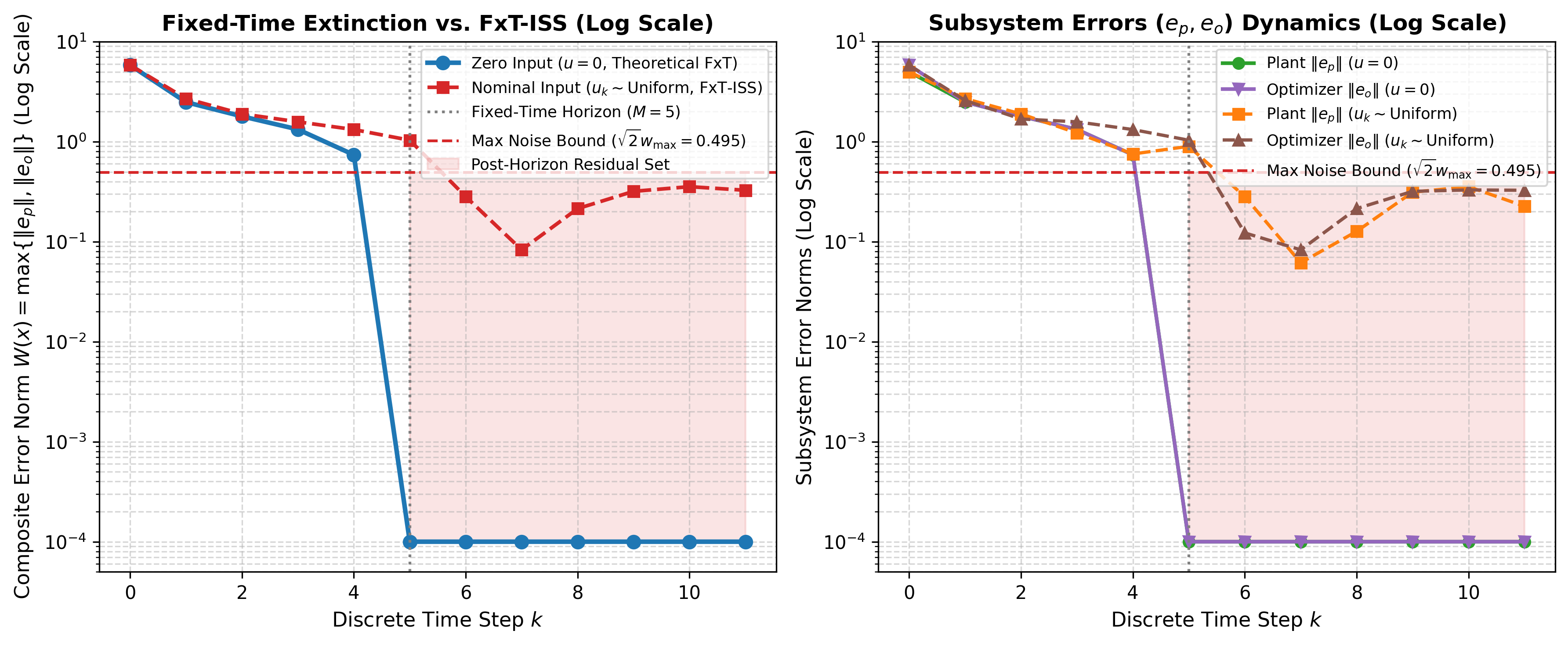
Thus, the one-step and finite-horizon conditions hold with $\rho_{p}=0$ , $\sigma_{po}(s)=(1+\|X\|)s$ , $\gamma_{po}(s)=\|X\|s$ , and $\gamma_{p}(s)=(\|XH^{-1}\|+1)s$ . In particular, $\sigma_{po}\in\mathcal{K}_{\infty}$ even when $X=0$ . It remains to verify the finite-horizon small-gain. Since $\gamma_{op}\equiv 0$ , the perturbed loop-gain maps satisfy $\Gamma_{o,r}(s)=\gamma_{op}\left(\gamma_{po}(s)+\gamma_{p}(r)\right)+\gamma_{o}(r)=\gamma_{o}(r)$ , and $\Gamma_{p,r}(s)=\gamma_{po}\left(\gamma_{op}(s)+\gamma_{o}(r)\right)+\gamma_{p}(r)=\gamma_{po}(\gamma_{o}(r))+\gamma_{p}(r)$ . Both bounds are independent of $s$ . Therefore, (28) holds with $N=1$ and $\vartheta_{o}(r):=\gamma_{o}(r)=\|H^{-1}\|r$ , $\vartheta_{p}(r):=\gamma_{po}(\gamma_{o}(r))+\gamma_{p}(r)=\left(\|X\|\|H^{-1}\|+\|XH^{-1}\|+1\right)r$ . It follows from Theorem 2 that the lifted feedback-optimization system (35)–(36) is FxT-ISS. Figure 2 shows a simulation of the closed-loop system.

V Proofs

V-A Proof of Proposition 1:

It suffices to establish the equivalence between conditions (4) and (6). To show necessity, suppose that $V$ is a finite-horizon FxT-ISS Lyapunov function. Then, by definition, there exist $\rho_{0}\in[0,1)$ and $\sigma\in\mathcal{K}_{\infty}$ such that (4) holds. Choose any $\rho\in(\rho_{0},1)$ and define $\chi(r):=\frac{\sigma(r)}{\rho-\rho_{0}}\in\mathcal{K}_{\infty}$ . If $V(x)\geq\chi(\|u\|)$ , then $\sigma(\|u\|)\leq(\rho-\rho_{0})V(x)$ . Consequently,

V(x^{+})\leq\rho_{0}V(x)+(\rho-\rho_{0})V(x)=\rho V(x).

(40)

Thus, the implication-type condition holds.

To show sufficiency, suppose now that conditions (3) and (5) hold. If $V(x)\geq\chi(\|u\|)$ , then condition (6) directly gives $V(x^{+})\leq\rho V(x)$ . On the other hand, if $V(x)<\chi(\|u\|)$ , define for $r\geq 0$ :

\widehat{\sigma}(r):=\max\left\{V(g(x,u)):V(x)\leq\chi(r),\ \|u\|\leq r\right\}.

The function $\widehat{\sigma}(r)$ is well defined and finite. Indeed, from (3) we have that $V(x)\leq\chi(r)$ implies $|x|_{\mathcal{A}}\leq\alpha_{1}^{-1}(\chi(r))$ . Since $\mathcal{A}$ is compact, the set $\left\{x\in\mathbb{R}^{n}:|x|_{\mathcal{A}}\leq\alpha_{1}^{-1}(\chi(r))\right\}$ is compact. Hence, the set $\left\{(x,u):V(x)\leq\chi(r),\ \|u\|\leq r\right\}$ is compact. Since $g$ and $V$ are continuous, the maximum defining $\widehat{\sigma}(r)$ exists and is finite. Moreover, $\widehat{\sigma}(0)=0$ . Indeed, $\chi(0)=0$ , and therefore $V(x)\leq\chi(0)$ implies $V(x)=0$ . Applying condition (6) with $u=0$ gives

V(g(x,0))\leq\rho V(x)=0.

Thus, $V(g(x,0))=0$ . By continuity of $g$ and $V$ , compactness of $\mathcal{A}$ , and the comparison bounds, it follows that $\widehat{\sigma}(r)\to 0\qquad\text{as }r\to 0^{+}$ . Furthermore, $\widehat{\sigma}$ is nondecreasing and finite on $\mathbb{R}_{\geq 0}$ . Hence, there exists $\sigma\in\mathcal{K}_{\infty}$ such that $\widehat{\sigma}(r)\leq\sigma(r)$ , for all $r\geq 0$ . Now, if $V(x)<\chi(\|u\|)$ , then, taking $r=\|u\|$ , we get

V(g(x,u))\leq\widehat{\sigma}(\|u\|)\leq\sigma(\|u\|).

Combining the two cases gives $V(g(x,u))\leq\max\left\{\rho V(x),\sigma(\|u\|)\right\}$ . Finally, using $\max\{a,b\}\leq a+b$ for all $a,b\geq 0$ , we obtain $V(g(x,u))\leq\rho V(x)+\sigma(\|u\|)$ . Thus, $V$ is a finite-horizon FxT-ISS Lyapunov function. $\blacksquare$

V-B Proof of Theorem 1 :

Let $V_{j}:=V(x(j))$ and $U_{j}:=\|u\|_{[0,j-1],\infty}$ . From (4), we have $V_{j+1}\leq\rho V_{j}+\sigma(\|u(j)\|)$ . Iterating this inequality yields $V_{j}\leq\rho^{j}V_{0}+\sum_{k=0}^{j-1}\rho^{j-1-k}\sigma(\|u(k)\|)$ . Since $\sigma$ is increasing,

V_{j}\leq\rho^{j}V_{0}+\left(\sum_{k=0}^{j-1}\rho^{k}\right)\sigma(U_{j}).

(41)

For $0\leq j<M$ , define $C_{M}:=\sum_{k=0}^{M-1}\rho^{k}=\frac{1-\rho^{M}}{1-\rho}$ . Then $V_{j}\leq\rho^{j}V_{0}+C_{M}\sigma(U_{j}),~~0\leq j<M$ . Using (3), we have $V_{0}\leq\alpha_{2}(|x(0)|_{\mathcal{A}})$ and hence

V_{j}\leq\rho^{j}\alpha_{2}(|x(0)|_{\mathcal{A}})+C_{M}\sigma(U_{j}),\qquad 0\leq j<M.

(42)

For $j\geq M$ , applying (5) at time $j-M$ gives

V_{j}=V\!\left(G_{M}(x(j-M),u(j-M),\ldots,u(j-1))\right)

(43)

and therefore

V_{j}\leq\gamma\!\left(\max_{j-M\leq k\leq j-1}\|u(k)\|\right).

(44)

Since $\max_{j-M\leq k\leq j-1}\|u(k)\|\leq U_{j}$ , and $\gamma$ is increasing, we get $V_{j}\leq\gamma(U_{j})$ for all $j\geq M$ . Choose $\bar{\rho}\in(\rho,1)$ and define

b(s,j):=\begin{cases}\bar{\rho}^{j}\alpha_{2}(s),&0\leq j<M,\\ 0,&j\geq M.\end{cases}

and $\eta(r):=\max\left\{C_{M}\sigma(r),\gamma(r)\right\}$ . Combining (42) and $V_{j}\leq\gamma(U_{j})$ for all $j\geq M$ gives,

V_{j}\leq b(|x(0)|_{\mathcal{A}},j)+\eta(U_{j}),~~\forall~j\geq 0.

(45)

Using the lower bound in (3), we get $\alpha_{1}(|x(j)|_{\mathcal{A}})\leq b(|x(0)|_{\mathcal{A}},j)+\eta(U_{j})$ . Therefore,

|x(j)|_{\mathcal{A}}\leq\alpha_{1}^{-1}\!\left(b(|x(0)|_{\mathcal{A}},j)+\eta(U_{j})\right).

Using the inequality $\alpha_{1}^{-1}(a+b)\leq\max\left\{\alpha_{1}^{-1}(2a),\alpha_{1}^{-1}(2b)\right\}$ , for $a,b\geq 0$ , we obtain

|x(j)|_{\mathcal{A}}\leq\max\left\{\beta(|x(0)|_{\mathcal{A}},j),\chi(U_{j})\right\},

(46)

where $\beta(s,j):=\alpha_{1}^{-1}(2b(s,j))$ and $\chi(r):=\alpha_{1}^{-1}(2\eta(r))$ . Since $0<\bar{\rho}<1$ , the function $\beta(\cdot,j)$ belongs to $\mathcal{K}$ for every $j<M$ , $\beta(s,\cdot)$ is nonincreasing, and $\beta(s,j)=0$ for every $j\geq M$ . Thus, $\beta\in\mathcal{KL}_{\mathrm{FxT}}$ and $\chi\in\mathcal{K}_{\infty}$ , which proves the claim. $\blacksquare$

V-C Proof of Proposition 2

It suffices to show that $V$ satisfies inequalities (4) and (5).

We first show that $V$ satisfies (4). Since $\psi\in\mathcal{E}_{\mathrm{FxT}}^{M}$ , by [19, Lemma 1] there exist $\varepsilon>0$ and $H<\infty$ such that: (a) $\psi(s)\geq s$ , for all $0\leq s\leq\varepsilon$ , and (b) $\psi(s)\geq s-H$ for all $s\geq 0$ . Moreover, (c) for every $s\geq 2H$ , we have that $\frac{\psi(s)}{s}\geq 1-\frac{H}{s}\geq\frac{1}{2}$ . Moreover, since $\psi$ is continuous and positive definite, the map $s\mapsto\psi(s)/s$ is continuous and strictly positive on every compact subset of $(0,\infty)$ . Hence, whenever $\varepsilon<2H$ , the quantity $c_{0}:=\min_{s\in[\varepsilon,2H]}\frac{\psi(s)}{s}$ i s well defined and satisfies $c_{0}>0$ . Combining this fact with properties (a) and (c), there exists a constant $c\in(0,1]$ such that $\psi(s)\geq cs$ , for all $s\geq 0$ . For example, if $\varepsilon<2H$ , one may take $c:=\min\left\{\frac{1}{2},c_{0}\right\}$ . If $\varepsilon\geq 2H$ , one may simply take $c=1/2$ . Let $\varrho:=1-c\in[0,1)$ . Then, for every $s\geq 0$ ,

\min\{\psi(s),s\}\geq cs=(1-\varrho)s.

Therefore, the extinction-based dissipation inequality gives

	$\displaystyle V(x^{+})-V(x)$	$\displaystyle\leq-\min\{\psi(V(x)),V(x)\}+\rho(\|u\|)$
		$\displaystyle\leq-(1-\varrho)V(x)+\rho(\|u\|).$		(47)

Thus, $V$ satisfies (4). To prove (5), define $g_{\psi}(s):=[s-\psi(s)]_{+}$ , $h_{\psi}(s):=\max_{0\leq\tau\leq s}g_{\psi}(\tau)$ . Since $\psi\in\mathcal{E}_{\mathrm{FxT}}^{M}$ , it follows that $h_{\psi}^{M}(s)=0$ for all $s\geq 0$ . Fix $k\in\mathbb{Z}_{\geq 0}$ and let $v_{j}:=V(x(k+j))$ , $r:=\|u\|_{[k,k+M-1],\infty}$ . For $j\in\{0,\ldots,M-1\}$ , the extinction-based dissipation inequality gives

	$\displaystyle v_{j+1}$	$\displaystyle\leq v_{j}-\min\{\psi(v_{j}),v_{j}\}+\rho(r)=g_{\psi}(v_{j})+\rho(r)$
		$\displaystyle\leq h_{\psi}(v_{j})+\rho(r).$		(48)

For each $r\geq 0$ , define $T_{r}(s):=h_{\psi}(s)+\rho(r)$ . Since $h_{\psi}$ is nondecreasing, repeated application of (48) yields $v_{M}\leq T_{r}^{M}(v_{0})$ . The extinction property implies that $h_{\psi}$ is globally bounded. Let $H:=\sup_{s\geq 0}h_{\psi}(s)<\infty$ . Hence, $T_{r}(s)\leq H+\rho(r)$ , for all $s\geq 0$ . Consequently, $T_{r}^{M}(s)\leq T_{r}^{M-1}(H+\rho(r))$ , for all $s\geq 0$ . Define $\Gamma(r):=T_{r}^{M-1}(H+\rho(r))$ . The map $\Gamma$ is continuous because $h_{\psi}$ and $\rho$ are continuous. Moreover, $\Gamma(0)=h_{\psi}^{M-1}(H)$ . Since $H$ belongs to the range closure of $h_{\psi}$ and $h_{\psi}^{M}\equiv 0$ , continuity of $h_{\psi}^{M-1}$ gives $h_{\psi}^{M-1}(H)=0$ . Thus, $\Gamma(0)=0$ , and therefore there exists $\sigma\in\mathcal{K}_{\infty}$ such that $\Gamma(r)\leq\sigma(r)$ , for all $r\geq 0$ . It follows that

V(x(k+M))=v_{M}\leq\sigma\!\left(\|u\|_{[k,k+M-1],\infty}\right),

which is precisely inequality (5). $\blacksquare$

V-D Proof of Theorem 2

Let $v_{i}(k):=V_{i}(x_{i}(k))$ , $i\in\{1,2\}$ , and, for integers $0\leq k\leq L$ , define $S_{i}^{L}(k):=\max_{k\leq\ell\leq L}v_{i}(\ell)$ . Also, let $U_{k,L}:=\|u\|_{[k,L-1],\infty}$ . Fix $L\geq k+M$ . For every $q\in\{k+M,\ldots,L\}$ , applying (25) at time $q-M$ gives

	$\displaystyle v_{i}(q)$	$\displaystyle\leq\gamma_{ij}\left(\max_{q-M\leq\ell<q}v_{j}(\ell)\right)+\gamma_{i}\left(\\|u_{i}\\|_{[q-M,q-1],\infty}\right)$
		$\displaystyle\leq\gamma_{ij}(S_{j}^{L}(k))+\gamma_{i}(U_{k,L}).$

Taking the maximum over $q\in\{k+M,\ldots,L\}$ yields

S_{i}^{L}(k+M)\leq\gamma_{ij}(S_{j}^{L}(k))+\gamma_{i}(U_{k,L}).

(49)

Suppose now that $L\geq k+2M$ . Applying (49) successively to both subsystems gives

	$\displaystyle S_{1}^{L}(k+2M)$	$\displaystyle\leq\gamma_{12}(S_{2}^{L}(k+M))+\gamma_{1}(U_{k,L})$
		$\displaystyle\leq\gamma_{12}\left(\gamma_{21}(S_{1}^{L}(k))+\gamma_{2}(U_{k,L})\right)+\gamma_{1}(U_{k,L})$
		$\displaystyle=\Gamma_{1,U_{k,L}}(S_{1}^{L}(k)).$

Similarly, $S_{2}^{L}(k+2M)\leq\Gamma_{2,U_{k,L}}(S_{2}^{L}(k))$ . Iterating these inequalities $N$ times yields, whenever $L\geq k+2NM$ ,

S_{i}^{L}(k+2NM)\leq\Gamma_{i,U_{k,L}}^{N}(S_{i}^{L}(k))\leq\vartheta_{i}(U_{k,L}),\qquad i\in\{1,2\},

(50)

where the last inequality follows from (28). Let $K:=2NM$ . For any $j\geq K$ , choose $k=0$ and $L=j$ in (50). Since $j\in[K,j]$ , it follows that

v_{i}(j)\leq S_{i}^{j}(K)\leq\vartheta_{i}(U_{j}),\qquad U_{j}:=\|u\|_{[0,j-1],\infty}.

(51)

Thus, after the uniform horizon $K$ , the bound is independent of the initial condition. In particular, for $u=0$ , since $\vartheta_{i}(0)=0$ , $v_{i}(j)=0$ , for $j\geq K$ . It remains to bound the transient $0\leq j<K$ . Define $R(j):=\max\{v_{1}(j),v_{2}(j)\}$ , and let $\rho:=\max\{\rho_{1},\rho_{2}\}$ , $\sigma(s):=\max\{\sigma_{12}(s),\sigma_{21}(s)\}$ , $\sigma_{u}(s):=\max\{\sigma_{1}(s),\sigma_{2}(s)\}$ . It follows from (24) that

R(j+1)\leq\rho R(j)+\sigma(R(j))+\sigma_{u}(|u(j)|).

(52)

Moreover, define $\overline{\alpha}(s):=\max\left\{\overline{\alpha}_{1}(s),\overline{\alpha}_{2}(s)\right\}$ . Then, condition (23) gives $R(0)\leq\overline{\alpha}(|x(0)|)$ . Since $K$ is finite, repeated application of (52) yields, for each $0\leq j<K$ , functions $p_{j}\in\mathcal{K}_{\infty}$ and $q_{j}\in\mathcal{K}$ such that

R(j)\leq p_{j}(|x(0)|)+q_{j}(U_{j}).

(53)

Define $\underline{\alpha}(s):=\min_{i\in\{1,2\}}\underline{\alpha}_{i}\left(\frac{s}{\sqrt{2}}\right)$ . Since at least one component satisfies $|x_{i}(j)|\geq|x(j)|/\sqrt{2}$ , we have $\underline{\alpha}(|x(j)|)\leq R(j)$ . Hence, using (53) and $\underline{\alpha}^{-1}(a+b)\leq\underline{\alpha}^{-1}(2a)+\underline{\alpha}^{-1}(2b)$ , we obtain

|x(j)|\leq b_{j}(|x(0)|)+c_{j}(U_{j}),\qquad 0\leq j<K,

(54)

where $b_{j}(s):=\underline{\alpha}^{-1}(2p_{j}(s))$ , $c_{j}(s):=\underline{\alpha}^{-1}(2q_{j}(s))$ . For $0\leq j<K$ , define $\beta(s,j):=\max_{j\leq\ell<K}b_{\ell}(s)$ , and set $\beta(s,j):=0$ , for $j\geq K$ . By construction, $\beta(\cdot,j)\in\mathcal{K}$ for $j<K$ , $\beta(s,\cdot)$ is nonincreasing, and $\beta(s,j)=0$ for every $s\geq 0$ and $j\geq K$ . Therefore, $\beta\in\mathcal{KL}_{\rm FxT}$ . To construct the input gain, define $c(s):=\max_{0\leq j<K}c_{j}(s).$ Moreover, from (51), we have $|x_{i}(j)|\leq\underline{\alpha}_{i}^{-1}\bigl(\vartheta_{i}(U_{j})\bigr)$ , for $j\geq K$ . Consequently, $|x(j)|\leq d(U_{j})$ for $j\geq K$ , where $d(s):=\left(\sum_{i=1}^{2}\left[\underline{\alpha}_{i}^{-1}\bigl(\vartheta_{i}(s)\bigr)\right]^{2}\right)^{1/2}$ . Let $\chi\in\mathcal{K}$ be any class- $\mathcal{K}$ majorant of $\max\{c,d\}$ . Combining (54) with the post-horizon estimate then gives

|x(j)|\leq\beta(|x(0)|,j)+\chi(U_{j}),\qquad j\in\mathbb{Z}_{\geq 0}.

Finally, using $a+b\leq\max\{2a,2b\}$ for $a,b\geq 0$ , and defining $\widetilde{\beta}(s,j):=2\beta(s,j)$ , and $\widetilde{\chi}(s):=2\chi(s)$ , we obtain

|x(j)|\leq\max\left\{\widetilde{\beta}(|x(0)|,j),\widetilde{\chi}\left(\|u\|_{[0,j-1],\infty}\right)\right\}.

(55)

Since $\widetilde{\beta}\in\mathcal{KL}_{\rm FxT}$ , the origin of (22) is FxT-ISS. $\blacksquare$

VI Conclusions

This paper introduced a finite-horizon Lyapunov framework for studying fixed-time ISS in discrete-time systems. The proposed conditions capture the uniform loss of dependence on the initial state after a finite number of iterations, while allowing this property to arise from the multi-step structure of the dynamics. We also established a finite-horizon small-gain theorem for interconnected systems, providing conditions under which this property is preserved under feedback interconnections. The framework was illustrated through examples involving deadbeat dynamics, distributed consensus, and finite-step optimization.

References

[1] Z. Jiang and Y. Wang (2001) Input-to-state stability for discrete-time nonlinear systems. Automatica 37 (6), pp. 857–869. Cited by: §I.
[2] C. M. Kellet and A. R. Teel (2004) Smooth Lyapunov functions and robustness of stability for difference inclusions. Systems & Control Letters 52 (5), pp. 395–405. Cited by: §I.
[3] R. Geiselhart and N. Noroozi (2017) Equivalent types of iss lyapunov functions for discontinuous discrete-time systems. Automatica 84, pp. 227–231. Cited by: §I.
[4] W. M. Haddad and V. Chellaboina (2008) Nonlinear Dynamical Systems and Control: a Lyapunov-Based Approach. Princeton U. Press. Cited by: §I.
[5] V. Andrieu, L. Praly, and A. Astolfi (2008) Homogeneous approximation, recursive observer design, and output feedback. SIAM Journal on control and optimization 47 (4), pp. 1814–1850. Cited by: §I.
[6] F. Lopez-Ramirez, D. Efimov, A. Polyakov, and W. Perruquetti (2019) Conditions for fixed-time stability and stabilization of continuous autonomous systems. Syst. and Cont. Letters 129, pp. 26–35. Cited by: §I, §III.
[7] A. Polyakov (2011) Nonlinear feedback design for fixed-time stabilization of linear control systems. IEEE transactions on Automatic Control 57 (8), pp. 2106–2110. Cited by: §I.
[8] H. Ríos, D. Efimov, J. A. Moreno, W. Perruquetti, and J. G. Rueda-Escobedo (2017) Time-varying parameter identification algorithms: finite and fixed-time convergence. IEEE Transactions on Automatic Control 62 (7), pp. 3671–3678. Cited by: §I.
[9] J. I. Poveda, M. Krstić, and T. Başar (2022) Fixed-time nash equilibrium seeking in time-varying networks. IEEE Transactions on Automatic Control 68 (4), pp. 1954–1969. Cited by: §I.
[10] J. I. Poveda and M. Krstić (2021) Nonsmooth extremum seeking control with user-prescribed fixed-time convergence. IEEE Transactions on Automatic Control 66 (12), pp. 6156–6163. Cited by: §I.
[11] K. Garg, M. Baranwal, R. Gupta, and M. Benosman (2022) Fixed-time stable proximal dynamical system for solving mvips. IEEE Transactions on Automatic Control 68 (8), pp. 5029–5036. Cited by: §I.
[12] N. Noroozi, R. Geiselhart, L. Grüne, and F. R. Wirth (2020) Control of discrete-time nonlinear systems via finite-step control lyapunov functions. Systems & Control Letters 138, pp. 104631. Cited by: §I.
[13] R. Geiselhart and F. R. Wirth (2016) Relaxed iss small-gain theorems for discrete-time systems. SIAM Journal on Control and Optimization 54 (2), pp. 423–449. Cited by: §I.
[14] J. Lee and W. M. Haddad (2023) Fixed time stability and optimal stabilisation of discrete autonomous systems. International Journal of Control 96 (9), pp. 2341–2355. Cited by: §I, §I.
[15] F. Tatari and H. Modares (2023) Deterministic and stochastic fixed-time stability of discrete-time autonomous systems. IEEE/CAA Journal of Automatica Sinica 10 (4), pp. 945–956. Cited by: §I, §I.
[16] Y. Mo and S. Dasgupta (2022) Small gain conditions for finite time input-to-state stability of interconnected discrete time systems. In Conference on Decision and Control, pp. 7714–7719. Cited by: §I.
[17] F. Mazenc and M. Malisoff (2024) Fixed-time input-to-state stabilization of discrete-time systems. IEEE Control Systems Letters 8, pp. 2625–2630. Cited by: §I.
[18] Y. Mo, W. Yu, and S. Dasgupta (2024) A lyapunov-based small-gain theorem for finite time input-to-state stablity of discrete time infinite networks. In 2024 IEEE 63rd Conference on Decision and Control (CDC), pp. 5120–5125. Cited by: §I.
[19] S. Rubaiyat and J. I. Poveda. (2026) Fixed-time iss for interconnected discrete-time systems, part i: extinction-based lyapunov conditions. Submitted to American Control Conference. Cited by: §I, §III-B, §III-B, §V-C, Definition 3.
[20] M. Tang, M. Krstic, and J. Poveda (2026) A lyapunov-based small-gain theorem for fixed-time stability. In 2026 American Control Conference (ACC), pp. 3711–3718. Cited by: §I.
[21] M. Tang, M. Krstic, and J. Poveda (2026) A lyapunov-based small-gain theorem for fixed-time iss: theory, optimization, and games. IEEE Transactions on Automatic Control, to appear. Cited by: §I.

	$\displaystyle W(T^{\ell}(T(x)+u))$	$\displaystyle\leq W(T^{\ell}(T(x)))+2\\|T^{\ell}(T(x)+u)$
		$\displaystyle~~~~-T^{\ell}(T(x))\\|_{\infty}$
		$\displaystyle\leq W(T^{\ell+1}(x))+2\\|u\\|_{\infty}.$

Fixed-Time ISS for Interconnected Discrete-Time Systems, Part II: Finite-Horizon Lyapunov Functions