Mean Spatial Frequency Decoupling for Learning-Based Uplink-to-Downlink Covariance Conversion in FDD Massive MIMO
Thanks: This work has been submitted to the IEEE for possible publication. Copyright may be transferred without notice, after which this version may no longer be accessible.
Abstract
In frequency division duplexing (FDD) massive multiple-input multiple-output (MIMO) systems, the uplink (UL)-to-downlink (DL) channel covariance matrix (CCM) conversion problem is studied to relieve the heavy burden of DL training and feedback required for channel estimation. Learning-based methods perform well up to a certain array size, but for a fixed dataset size their accuracy deteriorates with the number of antennas, to the point where simple model-based methods outperform them. This paper identifies a key cause of this behavior and addresses it. The mean angle of arrival (AoA) induces a phase ramp along the lags of the CCM. Since the oscillation rate of this ramp grows with the number of antennas, a dataset of fixed size becomes increasingly sparse relative to the variation that must be captured. We propose estimating the slope of this ramp from the UL CCM separately and mapping it to the DL band in closed form, leaving the learner with a residual that is largely insensitive to the mean AoA, which substantially reduces the performance degradation with an increasing number of antennas. The proposed scheme, termed deramping, is a combination of pre- and post-processing steps that applies to learning-based conversion methods without altering their internal structure, as demonstrated on three structurally different learners. Simulation results show that deramping reduces the covariance estimation error of all three learners under uniform, Laplacian, and Gaussian angular power spectra, keeps the interpolation-based learners ahead of a model-based benchmark at large array sizes, and improves downlink channel estimation.
Index Terms:
Channel covariance matrix, massive MIMO, frequency division duplexing (FDD), covariance conversion, channel estimationI Introduction
Massive multiple-input multiple-output (MIMO) is of vital importance for 5G and beyond networks owing to its high spectral efficiency and low energy consumption [1]. Implementing it in frequency division duplexing (FDD) systems, however, is hampered by an excessive pilot and feedback overhead [2, 3], since the channel reciprocity of time division duplexing (TDD) systems does not hold for FDD systems [4] and the overhead grows with the number of base station antennas. Exploiting second-order channel statistics such as the channel covariance matrix (CCM) helps reduce this burden [5]. Several studies estimate the downlink (DL) CCM from the uplink (UL) CCM [6, 7, 8, 9, 10, 11, 12, 13], relying on the spatial reciprocity between the two bands [14], which gives them the same power angular spectrum (PAS). Learning-based conversion methods [8, 11, 13] can lose accuracy as the number of antennas grows for a fixed dataset size [13]. Under a small angular spread, the covariance can be approximated by a mean-angle phase term times an angular-spread term, which has been used for parametric DL covariance estimation [15]. A related model-based scheme applies a diagonal phase transformation at the dominant UL direction to the UL CCM [16], which adapts the mean-angle phase term to the DL band but leaves the angular-spread term unchanged. In instantaneous DL channel extrapolation, the path delays and angles shared by the two links have been extracted so that a neural network maps only the frequency-dependent path gains [17],and a path-oriented extrapolator that aligns each extracted path response has been proposed to improve generalization across environments [18]. Unlike these works, we remove the mean-angle phase term from both links before learning and restore it analytically afterwards, so that a learner maps only the angular-spread term. This requires neither resolvable paths nor a particular PAS model and leaves the learner unchanged.
The main contributions of this paper are as follows.
- •
We identify a key cause of the performance degradation of learning-based UL-to-DL CCM conversion with increasing array size. The mean spatial frequency, i.e., the centroid of the PAS in the domain, enters the CCM as a phase ramp whose phase at the th lag sweeps an interval of width , so a fixed-size training set covers the data ever more sparsely as the number of antennas grows. In terms of the error bound of [13, Theorem 2], this can be interpreted as a growth of , the distance from a test point to its nearest training neighbor, and removing the ramp before learning is expected to slow this growth, which is consistent with the reduced degradation observed in Section IV.
- •
We propose deramping, which removes the ramp from both links before learning and restores it analytically afterwards, since its slope scales exactly by the carrier frequency ratio [16]. The deramp and restore operations are exactly invertible for any estimate of the mean spatial frequency, so an estimation error only leaves a small residual slope for the learner, and setting the estimate to zero recovers the baseline method identically. The learner itself is left unchanged, and we demonstrate the scheme on three structurally different learners.
- •
It was shown in [13] that learning-based methods are outperformed by the sinc transformation [12] as grows. With deramping, the dictionary [8] and kernel interpolators [13] remain ahead of the sinc transformation at all tested array sizes, and the gains carry over to DL channel estimation and to non-uniform PAS models.
Notation. Bold lower-case and upper-case letters denote vectors and matrices, respectively. , , , and denote the transpose, Hermitian transpose, inverse, and trace, respectively.
II System Model
The system model of [13] is adopted, where the base station (BS) has a uniform linear array (ULA) of antennas serving single-antenna user equipment (UE). The carrier frequency and wavelength of the UL band are and , and those of the DL band are and . Their ratio is , and the antenna spacing is .
The wide sense stationary uncorrelated scattering (WSSUS) model is adopted as in [13]. The CCMs of the zero-mean, frequency-flat UL and DL channels are [13]
| (1) |
where is the channel vector, is the PAS, is its half-width, is the mean angle of arrival (AoA), and is the array response vector with and .
Each CCM is Hermitian and Toeplitz, and hence determined by its first column, whose th entry is
| (2) |
Defining the spatial frequency , (2) becomes
| (3) |
where is the PAS in the -domain.
III Downlink Covariance Estimation via Deramping
III-A Problem Formulation
Given training pairs , learning-based methods seek a mapping that generalizes to unseen UL CCMs. For a ULA with , the covariance lags can be factorized exactly as
| (4) |
The first factor is linear in phase with respect to the lag index , and we refer to it as the phase ramp. Its slope is set by the mean spatial frequency , defined as the centroid of the PAS in the domain . The second factor , which we call the residual, depends only on the shape of the PAS around . Since the PAS is reciprocal between the two links, the same governs both, and only the slope of the ramp scales with . The phase ramp dominates the variability of the CCM entries. As spans , the ramp phase of the th lag sweeps an interval of width . A fixed training set therefore covers the data ever more sparsely as grows. The two factors transform differently from UL to DL. The ramp phase scales exactly, , whereas the residual does not, because is the residual of the same PAS evaluated at the non-integer lag . A direct mapping must therefore handle two operations implicitly. For the ramp, it must scale an unwrapped phase by the non-integer factor , although each entry reveals only the wrapped sum of the ramp and residual phases. The number of wraps must thus be inferred from the entire vector. For the residual, it must interpolate a slowly varying function to non-integer lags, which is the part that actually requires learning. Since the residual is also largely insensitive to , this motivates estimating from the UL CCM, removing the ramp from both links before learning, and restoring it analytically afterwards.
III-B Estimation of the Mean Spatial Frequency
We estimate from the Bartlett spectrum [19], where denotes expressed in the -domain. Owing to the Toeplitz structure of the CCM, it can be computed directly from the UL lags as
| (5) |
is not the PAS itself but its convolution with the power pattern of the uniformly weighted array, , whose main lobe has width and whose sidelobes decay only as over the entire periodic -axis. The mean spatial frequency is the centroid of the PAS in the -domain. Computing the same centroid from over a full period, however, is unreliable. Since the -axis is periodic, the linear centroid depends on where the period is cut and is dominated by the slowly decaying sidelobes of . The circular centroid, in turn, reduces to the phase of the lag-1 entry, and hence uses only the correlation between adjacent antennas while discarding the rest of the aperture. We therefore restrict the centroid computation to the main-lobe region of :
- 1.
is evaluated on a uniform grid of points over via a zero-padded discrete Fourier transform, which improves the numerical accuracy of the peak and centroid but not the resolution.
- 2.
Let denote the peak of , and let be the connected region around it on which . We set ( dB), just above the first sidelobe of ( dB), so that covers the main lobe but not the sidelobes. The region is taken circularly and may wrap around .
- 3.
The estimate is the centroid of over , computed relative to the peak:
(6) where is measured along the circle.
No phase unwrapping is involved, since is exactly one period of for , and the estimator does not assume any particular PAS shape.
III-C Proposed Method
The proposed method wraps a learning-based UL-to-DL conversion method with a pre-processing and a post-processing stage, as summarized in Algorithm 1. The operation returns the estimate of the mean spatial frequency (MSF) of a UL CCM (Section III-B), and Deramp removes a phase ramp from a lag sequence:
| (7) |
We denote by the lags deramped with an estimate , which coincide with the residual in (4) when .
In the training stage, is estimated from the UL CCM of each training sample, and both the UL input and the DL target of that sample are deramped with this same estimate, the DL slope being scaled by as in (4). Using the UL estimate for the DL target is essential, because only the UL CCM is available at test time, and it keeps deramping and ramp restoration consistent. The deramped lags are stacked as real vectors in the same format as the baseline, so the learner is trained without modification.
In the test stage, the UL CCM is deramped with its own estimate , the learner predicts the DL residual, and the DL ramp is restored analytically before the DL CCM is assembled as the Hermitian Toeplitz matrix with first column .
IV Simulation Results


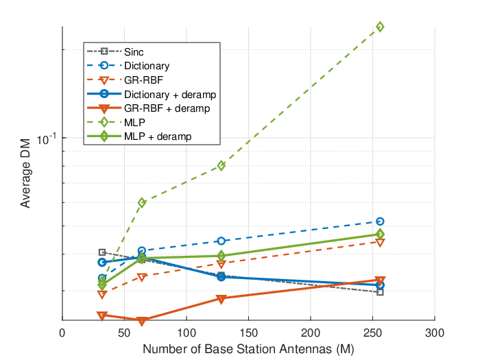


The experiments are conducted by varying at a fixed signal-to-noise ratio (SNR) and by varying the SNR at a fixed . Unless otherwise stated, , the SNR is dB, and the results are averaged over independent and identically distributed (i.i.d.) datasets. The simulation parameters are listed in Table I.
| Carrier frequencies | GHz, GHz |
|---|---|
| Antenna spacing | |
| Number of antennas | |
| SNR | dB |
| PAS | Uniform |
| Mean AoA | |
| PAS half-width | |
| Channel realizations per CCM | |
| Dataset size | , |
| GR-RBF [13] | , , |
| MLP hidden layers | , ReLU |
| Deramping | , |
The training and test datasets are generated as in [13]: each CCM is a sample covariance computed from channel realizations observed at the given SNR, projected onto the set of Hermitian positive semidefinite Toeplitz matrices using the method of [20].
We apply deramping to three learning-based methods: the dictionary-based interpolator of [8], the graph-regularized RBF kernel interpolator (GR-RBF) of [13] and a small multilayer perceptron (MLP) trained with Adam and early stopping. The MLP is not intended as a competitive method. It is included to test if the gains extend to neural networks. Each learner is evaluated with and without deramping under identical settings. As a model-based reference, we include the sinc transformation [12], which requires no training and was shown in [13] to outperform learning-based methods at large .
Performance is measured by the three metrics of [13]: normalized mean squared error (NMSE), correlation matrix distance (CMD), and deviation metric (DM). Fig. 1 shows the metrics as a function of at dB, and Fig. 2(a) shows the NMSE as a function of the SNR at . The CMD and DM versus SNR are omitted for brevity. Three observations follow.
- •
Deramping improves all three learners. At , it reduces the NMSE of the dictionary and GR-RBF methods by factors of and , respectively. For the MLP, whose mean is dominated by occasional training failures discussed below, we compare median values. The median NMSE of the MLP is reduced by a factor that grows monotonically with , from at to at . This is consistent with the phase ramp becoming the dominant source of variability as grows.
- •
The crossover with the sinc transformation is removed. Without deramping, the dictionary and GR-RBF methods fall behind the sinc transformation for and , respectively. With deramping, both remain below it at every tested , by a factor of about at . Their errors still increase from to , but the absolute increase is roughly halved, from to for GR-RBF and from to for the dictionary method. The MLP remains above the sinc transformation at every even with deramping, which is consistent with its role as a probe rather than a competitive method.
- •
The gain persists across SNR values and increases with the SNR. At low SNR, the error is dominated by the noise in the sample covariances rather than by the phase ramp, which limits the benefit of deramping.
| Laplacian | Gaussian | |||
|---|---|---|---|---|
| Method | Raw | Deramped | Raw | Deramped |
| Dictionary [8] | 0.0199 | 0.0090 | 0.0174 | 0.0058 |
| GR-RBF [13] | 0.0147 | 0.0089 | 0.0083 | 0.0048 |
| MLP | 0.3598 | 0.0401 | 0.1614 | 0.0129 |
| Sinc [12] | 0.0223 | 0.0198 | ||
The occasional failures of the deramped MLP stem from its per-feature standardization, which amplifies the noise in the nearly constant imaginary parts of the first residual lags. The interpolators do not standardize features and are unaffected.
To assess the dependence on the PAS model, Table II reports the NMSE at for the Laplacian and Gaussian PAS models of [13], averaged over datasets. Deramping improves all three learners under both models. The gains are – for GR-RBF, – for the dictionary method, and about an order of magnitude for the MLP, in the same order as under the uniform PAS. This is expected, since the factorization (4) holds for any PAS and the estimator (6) does not assume a particular PAS shape. Unlike the uniform case, the dictionary and GR-RBF methods already outperform the sinc transformation at under these models, and deramping widens the margin further. Deramping also narrows the gap between the dictionary and GR-RBF methods, from to under the Laplacian PAS and from to under the Gaussian PAS.
Since the DL CCM is ultimately used for DL channel estimation, we also evaluate the minimum mean squared error (MMSE) channel state information (CSI) estimation performance obtained with each DL CCM estimate. The DL CCMs are estimated at and dB SNR. After pilot transmission for DL CSI acquisition, the received signal at the user equipment (UE) is
| (8) |
where is the DL channel vector with covariance , contains the received symbols, the rows of are the pilot vectors, and is the noise vector. The MMSE DL CSI estimator is [15]
| (9) |
In the experiments, in (9) is replaced by the estimate obtained with each method. The rows of the pilot matrix are chosen to be orthogonal and scaled so that , which satisfies the total pilot power constraint with equality and requires . The pilot SNR is defined as , and the estimation performance is measured by the average of .
Fig. 2(b) and (c) show the performance for varying pilot SNR and number of pilot symbols , together with a genie-aided benchmark that uses the true DL CCM. For each learning-based method, deramping improves the channel estimation performance, so the gain in DL CCM estimation carries over to the application for which the DL CCM is ultimately needed.
V Conclusion
This paper proposes a general pre- and post-processing technique applicable to any learning-based UL-to-DL CCM conversion method. A major bottleneck of learning-based conversion is identified as the phase ramp produced by the mean spatial frequency. By decomposing the problem into estimating the mean spatial frequency and learning only the residual, we improve the CCM estimation performance of three learning-based methods under uniform, Laplacian, and Gaussian PAS models, as well as the resulting channel estimation performance. The performance deterioration with an increasing number of base station antennas for a constant dataset size is substantially reduced, and the interpolation-based learners no longer fall behind the model-based benchmark at large . Future work includes multi-cluster channels and other array geometries, such as the uniform rectangular array (URA), where the ramp becomes two-dimensional, and the uniform circular array (UCA), where the factorization must be reformulated.
Acknowledgment
The author used Anthropic’s Claude models as a research assistant. The tool suggested the decomposition on which the proposed method is based, drafted and revised parts of the simulation code, proposed the structure of Algorithm 1, drafted parts of the text, and revised the language, consistency, and formatting of all sections. All ideas were evaluated, corrected, and validated by the author through independent simulations, and several intermediate claims produced by the tool were found to be incorrect and discarded. The author designed the experiments, verified all results, and takes full responsibility for the content of this paper.
References
- [1] (2017) Massive MIMO networks: spectral, energy, and hardware efficiency. Found. Trends Signal Process. 11 (3-4), pp. 154–655. Cited by: §I.
- [2] (2016) Massive MIMO: ten myths and one critical question. IEEE Commun. Mag. 54 (2), pp. 114–123. Cited by: §I.
- [3] (2014) User grouping for massive MIMO in FDD systems: new design methods and analysis. IEEE Access 2, pp. 947–959. Cited by: §I.
- [4] (2020) FDD massive MIMO uplink and downlink channel reciprocity properties: full or partial reciprocity?. In Proc. IEEE Global Commun. Conf. (GLOBECOM), pp. 1–5. Cited by: §I.
- [5] (2018) Channel estimation for TDD/FDD massive MIMO systems with channel covariance computing. IEEE Trans. Wireless Commun. 17 (6), pp. 4206–4218. Cited by: §I.
- [6] (2001) Downlink channel covariance matrix (DCCM) estimation and its applications in wireless DS-CDMA systems. IEEE J. Sel. Areas Commun. 19 (2), pp. 222–232. Cited by: §I.
- [7] (2009) Conversion from uplink to downlink spatio-temporal correlation with cubic splines. In Proc. IEEE 69th Veh. Technol. Conf. (VTC Spring), pp. 1–5. Cited by: §I.
- [8] (2015) Channel covariance estimation in massive MIMO frequency division duplex systems. In Proc. IEEE Globecom Workshops, pp. 1–6. Cited by: 3rd item, §I, TABLE II, §IV.
- [9] (2019) FDD massive MIMO via UL/DL channel covariance extrapolation and active channel sparsification. IEEE Trans. Wireless Commun. 18 (1), pp. 121–135. Cited by: §I.
- [10] (2021) Channel covariance conversion and modelling using infinite dimensional Hilbert spaces. IEEE Trans. Signal Process. 69, pp. 3145–3159. Cited by: §I.
- [11] (2023) Downlink channel estimation for FDD massive MIMO using conditional generative adversarial networks. IEEE Trans. Wireless Commun. 22 (1), pp. 122–137. Cited by: §I.
- [12] (2023) Uplink to downlink channel covariance transformation in FDD systems. IEEE Trans. Signal Process. 71 (), pp. 3196–3212. External Links: Document Cited by: 3rd item, §I, TABLE II, §IV.
- [13] (2025) Downlink channel covariance matrix estimation via representation learning with graph regularization. Digit. Signal Process., pp. 105515. Cited by: 1st item, 3rd item, §I, §II, §II, TABLE I, TABLE II, §IV, §IV, §IV, §IV.
- [14] (2002) Spatial reciprocity of uplink and downlink radio channels in FDD systems. In Proc. COST 273 Technical Document TD(02)066, Cited by: §I.
- [15] (2017) Low-rank covariance-assisted downlink training and channel estimation for FDD massive mimo systems. IEEE transactions on wireless communications 16 (3), pp. 1935–1947. Cited by: §I, §IV.
- [16] (2023) Reciprocity evaluation based adaptive CCM reconstruction in FDD multi-antenna systems. Journal of Information and Intelligence 1 (2), pp. 148–155. Cited by: 2nd item, §I.
- [17] (2020) Downlink extrapolation for FDD multiple antenna systems through neural network using extracted uplink path gains. IEEE Access 8, pp. 67100–67111. Cited by: §I.
- [18] (2026) Generalizable learning for frequency-domain channel extrapolation under distribution shift. IEEE Transactions on Wireless Communications 25, pp. 9639–9655. Cited by: §I.
- [19] (2002) Optimum array processing: part iv of detection, estimation, and modulation theory. John Wiley & Sons. Cited by: §III-B.
- [20] (1994) Application of alternating convex projection methods for computation of positive Toeplitz matrices. IEEE Trans. Signal Process. 42 (7), pp. 1873–1875. Cited by: §IV.