Scaling Collider Event Generation with Residual-Quantized Tokens

Dan Godi Email: dan.godi@weizmann.ac.il Affiliation: Weizmann Institute of Science, Rehovot, Israel Dmitrii Kobylianskii Affiliation: Weizmann Institute of Science, Rehovot, Israel Eilam Gross Affiliation: Weizmann Institute of Science, Rehovot, Israel

Abstract

Full detector simulation and reconstruction of collider events are projected to become major bottlenecks at the High-Luminosity Large Hadron Collider, motivating the development of fast, ML-based surrogates. At the same time, LLMs have driven fast progress in generative discrete modeling: autoregressive transformers trained on tokenized data now represent the state of the art across a range of generative tasks. We extend the discrete modeling paradigm by introducing a particle-level generative model trained on residual-quantized full-event data. We demonstrate the ability of this model family to perform conditional generation from detector-stable particles; we study its scaling behavior across a range of dataset and model sizes, characterize the effects of repeated data exposure and demonstrate that token-level loss systematically predicts downstream physical fidelity. These results provide an empirical framework for scalable collider full-event generation based on residual-quantized representations.

I Introduction

At collider experiments, the growing sample size requirements for synthetic datasets are set to become a significant computational bottleneck. Projections for the High-Luminosity upgrade of the Large Hadron Collider (HL-LHC) estimate that, under current paradigms, full simulation tools will outstrip available compute resources, such that simulation and reconstruction of synthetic datasets will exceed the processing requirements of real data (ATLAS Collaboration, 2022, CMS Collaboration, 2026). Fast Simulation (FastSim) methods have emerged as solutions to this issue; these techniques use approximations to avoid modeling the full physical aspects of the simulation, hence consuming significantly fewer resources.

Over the past several years, Machine Learning (ML) has become a central tool in High Energy Physics (HEP), with deep learning algorithms now seeing wide adoption across the analysis chain (Butter et al., 2023, Krause et al., 2025, ATLAS Collaboration, 2026). Concurrently, advances in discrete sequence generation have established robust architectures and well-characterized scaling laws. These developments have been adopted in scientific applications, motivating recent formulations of HEP simulation as a discrete modeling problem.

Related work

Previous work in the field has focused on modeling at the jet (Birk et al., 2024, Golling et al., 2024, Amram et al., 2024, Bhimji et al., 2026) and calorimeter (Birk et al., 2025, Cardona-Giraldo et al., 2026) levels. More recently, generative approaches have been extended to conditional full-event simulation (Dreyer et al., 2026), but focusing on flow-matching techniques. Separately, neural scaling laws have been investigated in the context of jet tagging and generation (Vigl et al., 2026, Amram et al., 2026), building on broader developments in model and data scaling. In parallel with our work, Kakati et al. (2026) have explored a multimodal generative approach based on residual quantization in the single-jet setting.

In this work, we extend the discrete modeling paradigm to the full-event level. Full-event simulation is typically a two-stage process. Simulating the initial collision, subsequent interactions, and particle decays is relatively inexpensive, whereas simulating the detector response to stable particles and reconstructing the resulting signals is substantially more computationally intensive. The final output particles that are obtained after reconstruction are referred to as Particle Flow (PF) objects; these objects approximate the original set of particles entering the detector (Truth particles, TR), and are expected to maintain the physical properties and metrics used for downstream analysis. In principle, ML-based fast-simulation algorithms should be able to generate PF events without the need for TR conditioning, but conditional generation (and thus modeling of the detector response instead of the final output distribution) is strongly preferred for the ability to generalize to physical processes (rare or novel/theoretical) not seen during training. Since the model is conditioned on TR-level input, it learns the detector response itself as a physical map that is in principle independent of the process that produced the incoming particles, so a single surrogate can serve many signals and backgrounds rather than being re-tuned per analysis. While one could directly generate high-level observables, such as jets (sprays of particles clustered together), producing PF objects directly preserves the full event structure. This ensures compatibility with the existing downstream pipelines while providing a flexible foundation for developing new algorithms.

Contribution

Building on this full-event formulation, we show how the benefits of discrete residual-quantized representations transfer to point-cloud generation. We then study the scaling behavior of models spanning 10M to 1B parameters, characterize their dependence on model and dataset size, and examine the effects of repeated data exposure. We further demonstrate that the achieved loss is a powerful predictor of modeling performance at the physical scale: improvements in cross-entropy translate predictably into higher fidelity across particle-, jet-, and global event observables. These findings demonstrate that token-level scaling laws can reliably guide model capacity, dataset size, and compute allocation when designing generative surrogates for collider physics.

II Methods

Our approach factorizes event generation into two stages. First, a quantizer network is trained to map each truth or reconstructed particle to a short sequence of discrete tokens drawn from a learned codebook, resulting in a fixed vocabulary in which an event is represented as a sequence of integers. Second, an autoregressive transformer models the distribution over these token sequences, so that generation reduces to sampling the next token from a categorical distribution. Once a token sequence is sampled, it is passed back through the autoencoder’s decoder to recover continuous particle-level quantities. Decoupling the generative model from the data representation allows the transformer to operate on a compact discrete space, while the mapping to and from physical observables is handled by the separately trained fixed tokenizer.

II.1 Dataset

The model is trained and tested on several physical processes, from the CMS Open Data 2011 collection. Events are generated with Pythia 6.4.25 (Sjöstrand et al., 2008), passed through Geant4 (Agostinelli et al., 2003) simulation of the CMS detector, and subsequently reconstructed using the CMS Particle Flow algorithm (CMS Collaboration, 2009).

In each event we select from the dataset the set of generator-level final state TR particles and the corresponding set of PF particles. Each particle from these collections is described by its transverse momentum $p_{T}$ , its pseudorapidity $\eta$ and azimuthal angle $\phi$ , its class and the coordinates of its production vertex. Particles are categorized into one of five classes: charged hadron, electron, muon, neutral hadron, photon, and neutral PF particles have zeroed vertices (in real datasets the vertex of neutral particles can never be reconstructed since the tracking system only reads charged-particle deposits). Finally, the particles in each event are $p_{T}$ -ordered, from hardest to softest.
To improve momentum reconstruction and lessen tracker inefficiencies, we follow Dreyer et al. (2026) and require $p_{T}>1$ GeV for PF particles, and apply $p_{T}>0.25$ GeV cut on the TR set to reduce its cardinality.

Table 1: Datasets used for training and testing, in-distribution testing slices sum up to

50,000

events. Parton-level

p_{T}

ranges are shown for QCD samples.

Dataset	$p_{\mathrm{T}}^{\min}$ – $p_{\mathrm{T}}^{\max}$ [GeV]	Type	Training [evts]	Testing [evts]
$H\rightarrow 4\ell$	–	Out-of-distribution		$50{,}000$
$t\bar{t}$	–	In distribution	$9{,}361{,}338$	$28{,}263$
QCD	470–600	In distribution	$3{,}737{,}811$	$11{,}285$
QCD	600–800	In distribution	$3{,}462{,}168$	$10{,}452$
QCD	1000–1400	Out-of-distribution		$50{,}000$

The training dataset is made of a mixture of $t\bar{t}$ and QCD samples, available with high statistics. The model is subsequently tested on a mixture of statistically identical held-out samples, and a series of out-of-distribution samples of physical processes not seen during training (CMS Collaboration, 2016a, CMS Collaboration, 2016b, CMS Collaboration, 2016c, CMS Collaboration, 2016d, CMS Collaboration, 2016e). An overview is available in Table 1.

II.2 RQ-VAE

Tokenizer networks such as vector-quantized autoencoders (Oord et al., 2018) (VQ-VAEs) compress an input into a discrete latent vector (code). An encoder first maps an input $x$ to a continuous latent $z$ , which is then quantized against a learned codebook $\mathcal{C}=\{e_{k}\}^{K}_{k=1}$ by nearest-neighbor lookup, so that $x$ is represented by a single index $k=\mathcal{Q}(z;\mathcal{C})$ and decoded from $e_{k}$ :

\mathcal{Q}(z;\mathcal{C})=\mathrm{argmin}_{k\in\{1,\dots,K\}}||z-e_{k}||_{2},

(1)

The fidelity of this representation is limited by the codebook size $K$ : driving down the quantization error requires a finer partition of the latent space. In practice, large codebooks are difficult to train and suffer from codebook collapse, in which a small fraction of entries are ever selected and the effective capacity saturates below $K$ .

By representing $z$ with an ordered sequence of $M$ codes, residual quantization (Zeghidour et al., 2021) avoids this tradeoff. The effective codebook size increases to $K^{M}$ while avoiding having to scale $K$ as much. The latent is encoded by quantizing the running residual: starting from $r_{0}=z$ , at each depth $m=1,\dots,M$ we select the code that best approximates the current residual vector and subtract it. In other words, at each depth $m$ :

k_{m}=\mathcal{Q}(r_{m-1};\mathcal{C}_{m}),\qquad r_{m}\;=\;r_{m-1}-e^{m}_{k_{m}},

(2)

where $\mathcal{C}_{m}=\{e^{m}_{k}\}_{k=1}^{K}$ is the codebook at such depth. The input is thus mapped to the sequence of indices $(k_{1},\dots,k_{M})$ , and the quantized latent is recovered as the cumulative sum $\hat{z}=\sum_{m=1}^{M}e^{m}_{k_{m}}$ . The reconstructed input $\hat{x}=G(\hat{z})$ is produced by a decoder $G$ . The tokenizer consists of a self-attention transformer encoder $E$ (Vaswani et al., 2023), the residual-quantization module, and a transformer decoder $G$ , and is trained end-to-end using the reconstruction objective. Further details on architecture and training methods are available in the Appendix A.2.

Given the frozen tokenizer, each particle is mapped to its ordered sequence of $M$ residual codes such that an event of $N$ particles is flattened into a sequence of $NM$ tokens, event generation thus becomes a sequence-modeling problem.

II.3 Autoregressive Generative Model

The core model is a decoder-only transformer with causal self-attention and gated feed-forward networks (Shazeer, 2020). A single linear head maps the final hidden state at each position to a categorical distribution over the code vocabulary. Further details on architecture specifications and training procedure are reported in Appendix B.
We model the distribution over PFlow tokens autoregressively with the transformer, conditioned on the Truth-level event: both TR and PF events are tokenized by the same frozen RQ-VAE. The model’s input is the concatenation of the tokenized TR event and the tokenized PF event, with each section following its own [SOS] token; the Truth block thus acts as a prefix on which the target block is conditioned. The embedding of each token is the sum of three learned components: a shared embedding over the vocabulary of code indices, a depth embedding indexed by the residual level $m\in\{1,\dots,M\}$ , and a learnable linear projection of the corresponding codebook vector $e^{m}_{k}$ itself.

Since events have variable particle multiplicity, the number of reconstructed particles $N_{\text{PF}}$ is predicted directly from the pooled truth prefix by a feed forward network that is trained to predict logits for the different cardinality amounts. This target multiplicity is supplied to the model through an additional learned ”countdown” embedding that encodes the number of particles still to be generated at each position. The model is trained on next-token-prediction and cardinality objectives using a composite Cross-Entropy Loss function:

\mathcal{L}=\mathcal{L}^{\text{CE}}+\lambda_{\text{card}}\,\mathcal{L}^{\text{CE}}_{\text{card}}\,\,\,\,\,,\,\,\,\,\lambda_{\text{card}}=0.1

(3)

After training, to generate an event we tokenize the truth input, prefill it as the prefix, and sample the reconstructed multiplicity $N_{\text{PF}}$ from the cardinality head’s output distribution. We then autoregressively sample exactly $N_{\text{PF}}\cdot M$ tokens from the categorical distribution. The resulting token sequence is passed through the frozen RQ-VAE decoder to recover the particle-level quantities. Training and inference details are provided in Appendix B.

III Results

We evaluate the reconstruction and generation performance on particle, event, and jet-level quantities. Jets are reconstructed from collimated sprays of particles by clustering nearby constituents in the $\eta-\phi$ plane into composite objects commonly used for downstream analysis in collider experiments.

We use both the held-out in-distribution test set (QCD + $t\bar{t}$ ) and out-of-distribution datasets ( $H\rightarrow 4\ell$ and QCD $1000$ ) to test the model’s ability to generalize beyond physical processes seen during training. We examine feature distributions, and we also match generated (FastSim, FS) and PFlow particles and jets with Truth ones, using the Hungarian matching algorithm (Kuhn, 1955) with $\Delta R=\sqrt{\Delta\eta^{2}+\Delta\phi^{2}}$ as the cost function, and then evaluate the per-feature residual distributions.

The choice of evaluating on the residual sets is intentional: the conditional generation objective is to model the stochastic detector response and reconstruction. FastSim samples should be evaluated in terms of how well they reproduce the full simulation and reconstruction pipeline’s response to the incoming detector-stable particles, rather than their ability to deterministically reproduce the exact PFlow features.

III.1 Tokenizer fidelity and codebook utilization

Achieving good performance on the reconstruction objective is a required test of the fidelity of the discrete representation learned by the tokenizer network. The latent is quantized with $M=4$ residual stages (Eq. 2), and each codebook layer contains $K=8192$ 16-dimensional vectors, more details can be found in Appendix A.2. For each continuous feature, the joint distribution, over both TR and PF-level events in the test dataset, of the original and reconstructed values is shown in Figure 1, together with the particle class confusion matrix.

Refer to caption — Figure 1: Reconstructed features residual distribution, and particle-class confusion matrix. Vertex residuals are only computed for charged particles.

Next we examine how the available discrete representation capacity is utilized across the residual-quantization levels. Figure 9 (Appendix D) shows the code distribution at each depth $m$ . For each codebook, we also characterize its usage (i.e. the percentage of codes used at least once) and perplexity; metrics are reported in Table 2.

Table 2: Codebook usage and perplexity (PPL) at each residual depth

m

, for the three test datasets.

Dataset	Usage	Perplexity	Usage	Perplexity	Usage	Perplexity	Usage	Perplexity
	$m=1$		$m=2$		$m=3$		$m=4$
QCD + $t\bar{t}$	58.5%	4042	99.9%	5575	99.9%	4894	99.9%	4723
$H\rightarrow 4\ell$	58.2%	3338	99.3%	5382	99.4%	4797	99.6%	4662
QCD 1000	58.5%	3897	99.9%	5652	100.0%	4981	100.0%	4871

III.2 Generation Performance

We show the performance of the largest model configuration, trained for four epochs on the full dataset. A performance comparison to other ablations is shown in Table 10, in the Appendix D.

Particle-level

Residual distributions of particle-level features, for PF and FS particles matched to TR, are reported in Figure 2. The generated residual distributions closely track the corresponding PF distributions. The $\eta$ and $\phi$ marginals in Figure 10 (Appendix D) also reproduce the detector-dependent structure across the tested datasets.

Figure 2: Spectra of particle residual features for all three testing datasets. All histograms are normalized to unity; rows correspond to different datasets/processes while columns correspond to different observables.

Event-level

Event-level variables are a relevant test of the model’s ability to capture global event correlations, in particular in an autoregressive setting where the bulk of the generated structure follows from a subset of initially generated hard particles. For event-level metrics, we consider number of particles, missing transverse energy in the $x$ and $y$ directions and the scalar sum of particle $p_{T}$ . Residual distributions of these metrics are shown in Figure 3, and marginals are displayed in the appendix (Figure 12).

Figure 3: Spectra of event-level residual features for all three testing datasets. All histograms are normalized to unity; rows correspond to different datasets/processes while columns correspond to different observables.

Jet-level

We examine the kinematic properties of the clustered jets ( $p_{T}$ , $\eta$ , $\phi$ ) and the jet substructure quantities $C_{2}$ and $D_{2}$ (Larkoski et al., 2013, Larkoski et al., 2014). While inclusive marginal distributions test the overall kinematic phase-space coverage of the generated FS samples against target PF, residual distributions with respect to truth-matched jets evaluate the conditional response and resolution. In addition, the substructure observables test the effective modeling of intra-jet particle correlations and detector effects. Residual distributions for the selected variables are shown in Figure 4, and marginals in the appendix (Figure 11).

Figure 4: Spectra of residuals of jet-level features for all three testing datasets. The residuals are computed against matched truth jets. All histograms are normalized to unity; rows correspond to different datasets/processes while columns correspond to different observables.

III.3 Scaling study

We study how the generator model’s performance changes with model size, training-set size, and repeated data exposure. We evaluate the model on the token cross-entropy loss on the statistically identical set of held-out events and fit its dependence on these training variables. We then evaluate how scaling affects the generated distributions of physical observables.
A full overview of training ablations used for the study is available in Tables 3 and 4.

Table 3: Model configurations used in the scaling study. Each model is trained with eight data and repetition settings, giving 48 configurations.

Name	$\boldsymbol{d_{\text{model}}}$	Layers	Heads	$\boldsymbol{d_{\text{head}}}$	$\boldsymbol{d_{\text{ff}}}$	Total Params
10M	256	8	8	32	512	$9.83$ M
22M	384	10	8	48	768	$21.67$ M
41M	512	12	8	64	1,024	$40.75$ M
97M	768	14	12	64	1,536	$96.71$ M
187M	1,024	16	16	64	2,048	$186.87$ M
1B	2,048	24	32	64	4,096	$1{,}046.92$ M

Table 4: Data and repetition settings used in the scaling study. Each setting is applied to all six model sizes. Data fractions are subsampled from the full dataset, in order to preserve the same statistical properties.

Data fraction	Unique events	Epochs	PF tokens	Total tokens
3.3%	$546{,}523$	$1,\ 10,\ 30$	$324$ M	$749$ M
33.3%	$5{,}514{,}918$	$1,\ 3,\ 12$	$3.27$ B	$7.56$ B
100%	$16{,}561{,}317$	$1,\ 4$	$9.82$ B	$22.7$ B

III.3.1 Loss scaling

The fitted quantity is the held-out next-token-prediction (NTP) cross-entropy $\mathcal{L}$ , in nats. This is the token component of the objective defined in Section II.3; the cardinality term is excluded. First, we ignore data repetition and only consider fresh-data runs in which each event is only shown to the model once at most. In this regime, we fit the additive Chinchilla (Hoffmann et al., 2022) and coupled Skaling (Videau et al., 2026) forms that model the data-constraint free scaling behavior of the model family.

In settings such as detector simulation, generating MC training datasets can be an expensive endeavor. It is important to model the effects of data repetition on ML-based surrogates, and maximize the usefulness of the available synthetic datasets. To evaluate the effects of repeated data exposure, we also fit the "Prescriptive" repetition penalty introduced by Lovelace et al. (2026), and a custom combined form that applies this penalty to the Skaling coupled expression. We fit the measured losses by unweighted least squares. Table 5 reports the fitted $\alpha,\beta$ parameters and the exponents for compute-optimal allocation $a=\beta/(\alpha+\beta)$ and $b=\alpha/(\alpha+\beta)$ (Hoffmann et al., 2022), together with mean absolute percentage error (MAPE) and coefficient of determination $R^{2}$ , to indicate goodness-of-fit. Although the fitted parameters vary, all models predict similar values for the $a$ and $b$ optimal-scaling parameters. The full parameters are reported in Table 9, Appendix C.1.

Table 5: Fits of the neural scaling laws. Chinchilla and Skaling are fitted to the 18 single-epoch runs, the repetition-aware laws to all 48 runs. Uncertainties are

1\sigma

errors over refits with one run held-out.

Law	Functional form	$\alpha$	$\beta$	$a$	$b$	MAPE [%]	$R^{2}$
Chinchilla	$L_{\infty}+AN^{-\alpha}+BU^{-\beta}$	$0.42\,{\scriptstyle\pm 0.18}$	$0.62\,{\scriptstyle\pm 0.15}$	$0.60\,{\scriptstyle\pm 0.14}$	$0.40\,{\scriptstyle\pm 0.14}$	3.55	0.9695
Skaling	$L_{\infty}+\left(AN^{-\alpha}+BU^{-\beta}\right)^{k}$	$0.241\,{\scriptstyle\pm 0.052}$	$0.345\,{\scriptstyle\pm 0.070}$	$0.589\,{\scriptstyle\pm 0.048}$	$0.411\,{\scriptstyle\pm 0.048}$	1.17	0.9961
Prescriptive	$L_{\infty}+AN^{-\alpha}+B[U(1+R)]^{-\beta}+PR^{\delta}\left(\frac{N}{U^{\gamma}}\right)^{\kappa}$	$0.410\,{\scriptstyle\pm 0.092}$	$0.598\,{\scriptstyle\pm 0.036}$	$0.593\,{\scriptstyle\pm 0.074}$	$0.407\,{\scriptstyle\pm 0.074}$	2.47	0.9690
Custom	$L_{\infty}+\left(AN^{-\alpha}+B[U(1+R)]^{-\beta}\right)^{k}+PR^{\delta}\left(\frac{N}{U^{\gamma}}\right)^{\kappa}$	$0.273\,{\scriptstyle\pm 0.017}$	$0.349\,{\scriptstyle\pm 0.016}$	$0.561\,{\scriptstyle\pm 0.015}$	$0.439\,{\scriptstyle\pm 0.015}$	0.79	0.9967

Figure 5 compares the measured held-out losses with the fitted curves and the implied compute-optimal scaling of $N$ . Larger models overfit sooner on smaller datasets but achieve lower loss when sufficient unique data are available. Over the compute range covered by the single-epoch runs, the fitted compute-optimal model size remains below the largest models in our grid, indicating that the study is data-constrained. The isoFLOP-fitted analysis yields $N\propto C^{0.53}$ .

Figure 5: Left: each trained model’s NTP loss against its parameter count. The lines show the custom fitted law’s prediction for the given combination of dataset size and repetition. Right: compute-guided fit-predicted optimal scaling behaviors and isoFLOP curves minima. The methodology for recovering these minima is discussed in the Appendix C.2.

III.3.2 Scaling of physical metrics

It is not immediately obvious how modeling of the decoded physical variables correlates with a lower value of the NTP Loss. The model might produce token sequences that appear satisfactory on a surface level but produce nonsensical physical results once decoded. For this reason it is important to choose metrics that test both local and global features of the generated samples.

Global point-cloud metrics

First, we adopt a procedure similar to that of Amram et al. (2026) by comparing the NTP loss with the Sliced Wasserstein Distance (SWD) (Rabin et al., 2011, Bonneel et al., 2015) between FS and PF samples, but we instead evaluate on the particle-, event-, and jet-level residual feature manifolds. For each feature group, we subsample the point clouds and average the $W_{1}$ Wasserstein Distance over $256$ random projections after standardising every feature with the mean and standard deviation of the PF reference. We also include the statistical noise barrier obtained by computing the SWD between statistically identical samples.
In Figure 6 we plot the NTP loss for given checkpoints against the SWD on the given feature sets of the associated produced sample from the testing datasets. We find, by fitting a power law of the type:

\text{SWD}=a(\mathcal{L}-\mathcal{L}_{0})^{b}+\text{SWD}_{f}

(4)

that the loss achieved on the held-out test dataset is a very strong performance predictor on this global metric. Fit results and a visualization are available in Figure 6. Details on the full procedure are available in Appendix C.3.

Figure 6: Measured Sliced Wasserstein Distance for all valid (selection criteria in Appendix C.3) runs, and fitted law in the form of Equation 4. We include both final and intermediate checkpoints and show the fitted power law parameters for each feature.

Individual metrics

Observing scaling behavior on distributions of the individual output features is not a trivial task: modeling the marginal distributions of these is often easier and can result in differences that fall within two-sample noise. We find, however, that each one of the individual residual feature distributions exhibits scaling behavior, in the same form as Eq. 4, as the global feature manifolds, and that the achieved loss value is also a strong individual predictor of the fidelity of these generated physical metrics. In Figure 7 we check the one-dimensional $W_{1}$ Wasserstein Distance between the FastSim and PFlow residual distributions, and show the fit results across the different features. We find that improvements in achieved loss transfer to the individual features.

Figure 7: Per-feature

W_{1}

Wasserstein Distance between the PF and FS valid (selection criteria in Appendix C.3) residual distributions. We include both final and intermediate checkpoints and show the fitted power law parameters for each feature.

IV Conclusion

We apply discrete autoregressive modeling to conditional full-event simulation, demonstrating how residual-quantized representations of point-clouds enable generation of particle-level detector responses. By employing a frozen RQ-VAE tokenizer with an autoregressive transformer, we recover continuous particle-level outputs from discrete sequences while preserving the flexibility of full-event generation. We demonstrate the fidelity of the learned representation and evaluate the generated events across particle, event, and jet-level observables, including on physical processes not encountered during training.

We then study the scaling behavior of this model family across a range of model and dataset sizes, find that the next-token prediction loss exhibits familiar scaling characteristics, and that the effects of data repetition can be captured by a repetition-aware scaling law.

Our empirical results demonstrate a direct link between token-level modeling performance and the fidelity of generated physical observables. We show that the achieved next-token prediction loss is a strong predictor of both global distributional distances and individual metrics, with their relationship well described by a simple power law. These findings suggest that token-level scaling laws may provide a useful proxy for estimating downstream physical performance, validate residual-quantized autoregressive architectures for scalable simulation in high-energy physics and demonstrate how empirical scaling laws can guide compute allocation for ML surrogate models.

Acknowledgments

This work has been supported by the Minerva Grant, the Knell Family Institute for Artificial Intelligence, The Benoziyo Center for High Energy Physics, a BSF Grant, and the Krenter-Perinot Center for High Energy Particle Physics.

References

Agostinelli et al. (2003) S. Agostinelli, J. Allison, K. Amako, J. Apostolakis, H. Araujo, P. Arce, M. Asai, D. Axen, S. Banerjee, G. Barrand, F. Behner, L. Bellagamba, J. Boudreau, L. Broglia, A. Brunengo, H. Burkhardt, S. Chauvie, J. Chuma, R. Chytracek, G. Cooperman, G. Cosmo, P. Degtyarenko, A. Dell’Acqua, G. Depaola, D. Dietrich, R. Enami, A. Feliciello, C. Ferguson, H. Fesefeldt, G. Folger, F. Foppiano, A. Forti, S. Garelli, S. Giani, R. Giannitrapani, D. Gibin, J. J. Gómez Cadenas, I. González, G. Gracia Abril, G. Greeniaus, W. Greiner, V. Grichine, A. Grossheim, S. Guatelli, P. Gumplinger, R. Hamatsu, K. Hashimoto, H. Hasui, A. Heikkinen, A. Howard, V. Ivanchenko, A. Johnson, F. W. Jones, J. Kallenbach, N. Kanaya, M. Kawabata, Y. Kawabata, M. Kawaguti, S. Kelner, P. Kent, A. Kimura, T. Kodama, R. Kokoulin, M. Kossov, H. Kurashige, E. Lamanna, T. Lampén, V. Lara, V. Lefebure, F. Lei, M. Liendl, W. Lockman, F. Longo, S. Magni, M. Maire, E. Medernach, K. Minamimoto, P. Mora de Freitas, Y. Morita, K. Murakami, M. Nagamatu, R. Nartallo, P. Nieminen, T. Nishimura, K. Ohtsubo, M. Okamura, S. O’Neale, Y. Oohata, K. Paech, J. Perl, A. Pfeiffer, M. G. Pia, F. Ranjard, A. Rybin, S. Sadilov, E. Di Salvo, G. Santin, T. Sasaki, N. Savvas, Y. Sawada, S. Scherer, S. Sei, V. Sirotenko, D. Smith, N. Starkov, H. Stoecker, J. Sulkimo, M. Takahata, S. Tanaka, E. Tcherniaev, E. Safai Tehrani, M. Tropeano, P. Truscott, H. Uno, L. Urban, P. Urban, M. Verderi, A. Walkden, W. Wander, H. Weber, J. P. Wellisch, T. Wenaus, D. C. Williams, D. Wright, T. Yamada, H. Yoshida, and D. Zschiesche Geant4—a simulation toolkit. Nuclear Instruments and Methods in Physics Research Section A: Accelerators, Spectrometers, Detectors and Associated Equipment 506 (3), pp. 250–303. External Links: ISSN 0168-9002, Link, Document Cited by: §II.1.
Amram et al. (2024) O. Amram, L. Anzalone, J. Birk, D. A. Faroughy, A. Hallin, G. Kasieczka, M. Krämer, I. Pang, H. Reyes-Gonzalez, and D. Shih Aspen Open Jets: Unlocking LHC Data for Foundation Models in Particle Physics. arXiv. Note: arXiv:2412.10504 [hep-ph] External Links: Link, Document Cited by: §I.
Amram et al. (2026) O. Amram, D. A. Faroughy, T. Gerdes, A. Hallin, G. Kasieczka, M. Krämer, H. Reyes-Gonzalez, and D. Shih Neural scaling laws for jet generation. External Links: 2605.28940, Link Cited by: §I, §III.3.2.
ATLAS Collaboration (2022) ATLAS Collaboration ATLAS Software and Computing HL-LHC Roadmap. Technical report CERN, Geneva. External Links: Link Cited by: §I.
ATLAS Collaboration (2026) ATLAS Collaboration Transforming jet flavour tagging at ATLAS. Nature Communications 17 (1), pp. 541 (en). External Links: ISSN 2041-1723, Link, Document Cited by: §I.
Ba et al. (2016) J. L. Ba, J. R. Kiros, and G. E. Hinton Layer Normalization. arXiv. Note: arXiv:1607.06450 [stat.ML] External Links: Link, Document Cited by: §A.2.
Bhimji et al. (2026) W. Bhimji, C. Harris, V. Mikuni, and B. Nachman OmniLearned: A Foundation Model Framework for All Tasks Involving Jet Physics. Physical Review D 113 (3), pp. 032020. Note: arXiv:2510.24066 [hep-ph] External Links: ISSN 2470-0010, 2470-0029, Link, Document Cited by: §I.
Birk et al. (2025) J. Birk, F. Gaede, A. Hallin, G. Kasieczka, M. Mozzanica, and H. Rose OmniJet- $\alpha\_C$ : Learning point cloud calorimeter simulations using generative transformers. arXiv. Note: arXiv:2501.05534 [hep-ph] External Links: Link, Document Cited by: §I.
Birk et al. (2024) J. Birk, A. Hallin, and G. Kasieczka OmniJet- $\alpha$ : The first cross-task foundation model for particle physics. Machine Learning: Science and Technology 5 (3), pp. 035031. Note: arXiv:2403.05618 [hep-ph] External Links: ISSN 2632-2153, Link, Document Cited by: §I.
Bonneel et al. (2015) N. Bonneel, J. Rabin, G. Peyré, and H. Pfister Sliced and Radon Wasserstein Barycenters of Measures. Journal of Mathematical Imaging and Vision 1 (51), pp. 22–45. External Links: Link, Document Cited by: §III.3.2.
Butter et al. (2023) A. Butter, T. Plehn, S. Schumann, S. Badger, S. Caron, K. Cranmer, F. A. D. Bello, E. Dreyer, S. Forte, S. Ganguly, D. Gonçalves, E. Gross, T. Heimel, G. Heinrich, L. Heinrich, A. Held, S. Höche, J. N. Howard, P. Ilten, J. Isaacson, T. Janßen, S. Jones, M. Kado, M. Kagan, G. Kasieczka, F. Kling, S. Kraml, C. Krause, F. Krauss, K. Kröninger, R. K. Barman, M. Luchmann, V. Magerya, D. Maitre, B. Malaescu, F. Maltoni, T. Martini, O. Mattelaer, B. Nachman, S. Pitz, J. Rojo, M. Schwartz, D. Shih, F. Siegert, R. Stegeman, B. Stienen, J. Thaler, R. Verheyen, D. Whiteson, R. Winterhalder, and J. Zupan Machine Learning and LHC Event Generation. SciPost Physics 14 (4), pp. 079. Note: arXiv:2203.07460 [hep-ph] External Links: ISSN 2542-4653, Link, Document Cited by: §I.
Cardona-Giraldo et al. (2026) C. Cardona-Giraldo, C. Fanelli, J. Giroux, C. Granger, B. Nachman, and G. Sabin Generalizable Foundation Models for Calorimetry via Mixtures-of-Experts and Parameter Efficient Fine Tuning. arXiv. Note: arXiv:2603.28804 [physics.ins-det] External Links: Link, Document Cited by: §I.
CMS Collaboration (2009) CMS Collaboration Particle-Flow Event Reconstruction in CMS and Performance for Jets, Taus, and MET. Technical report CERN, Geneva. External Links: Link Cited by: §II.1.
CMS Collaboration (2016a) CMS Collaboration Simulated dataset GluGluToHToZZTo4L_M-125_7TeV-minloHJJ-pythia6-tauola in AODSIM format for 2011 collision data (SM Higgs). CERN Open Data Portal. External Links: Document, Link Cited by: §II.1.
CMS Collaboration (2016b) CMS Collaboration Simulated dataset QCD_Pt-1000to1400_TuneZ2_7TeV_pythia6 in AODSIM format for 2011 collision data (SM Exclusive). CERN Open Data Portal. External Links: Document, Link Cited by: §II.1.
CMS Collaboration (2016c) CMS Collaboration Simulated dataset QCD_Pt-470to600_TuneZ2_7TeV_pythia6 in AODSIM format for 2011 collision data (SM Exclusive). CERN Open Data Portal. External Links: Document, Link Cited by: §II.1.
CMS Collaboration (2016d) CMS Collaboration Simulated dataset QCD_Pt-600to800_TuneZ2_7TeV_pythia6 in AODSIM format for 2011 collision data (SM Exclusive). CERN Open Data Portal. External Links: Document, Link Cited by: §II.1.
CMS Collaboration (2016e) CMS Collaboration Simulated dataset TTJets_MSDecays_central_TuneZ2_7TeV-madgraph-tauola in AODSIM format for 2011 collision data (SM Inclusive). CERN Open Data Portal. External Links: Document, Link Cited by: §II.1.
CMS Collaboration (2026) CMS Collaboration CMS Offline Software and Computing for HL-LHC Conceptual Design Report. Technical report CERN, Geneva. External Links: Link, Document Cited by: §I.
Dao et al. (2022) T. Dao, D. Y. Fu, S. Ermon, A. Rudra, and C. Ré FLASHATTENTION: fast and memory-efficient exact attention with io-awareness. In Proceedings of the 36th International Conference on Neural Information Processing Systems, NIPS ’22, Red Hook, NY, USA. External Links: ISBN 9781713871088 Cited by: §A.2.
Dao (2023) T. Dao FlashAttention-2: faster attention with better parallelism and work partitioning. External Links: 2307.08691, Link Cited by: §A.2.
Dehghani et al. (2023) M. Dehghani, J. Djolonga, B. Mustafa, P. Padlewski, J. Heek, J. Gilmer, A. Steiner, M. Caron, R. Geirhos, I. Alabdulmohsin, R. Jenatton, L. Beyer, M. Tschannen, A. Arnab, X. Wang, C. Riquelme, M. Minderer, J. Puigcerver, U. Evci, M. Kumar, S. v. Steenkiste, G. F. Elsayed, A. Mahendran, F. Yu, A. Oliver, F. Huot, J. Bastings, M. P. Collier, A. Gritsenko, V. Birodkar, C. Vasconcelos, Y. Tay, T. Mensink, A. Kolesnikov, F. Pavetić, D. Tran, T. Kipf, M. Lučić, X. Zhai, D. Keysers, J. Harmsen, and N. Houlsby Scaling Vision Transformers to 22 Billion Parameters. arXiv. Note: arXiv:2302.05442 [cs] External Links: Link, Document Cited by: §A.2.
Dreyer et al. (2026) E. Dreyer, E. Gross, D. Kobylianskii, V. Mikuni, and B. Nachman Conditional deep generative models for simultaneous simulation and reconstruction of entire events. Physical Review D 113 (3), pp. 032005. External Links: Link, Document Cited by: §I, §II.1.
Fifty et al. (2024) C. Fifty, R. G. Junkins, D. Duan, A. Iyengar, J. W. Liu, E. Amid, S. Thrun, and C. Ré Restructuring Vector Quantization with the Rotation Trick. (en). External Links: Link Cited by: §A.2.
Golling et al. (2024) T. Golling, L. Heinrich, M. Kagan, S. Klein, M. Leigh, M. Osadchy, and J. A. Raine Masked Particle Modeling on Sets: Towards Self-Supervised High Energy Physics Foundation Models. Machine Learning: Science and Technology 5 (3), pp. 035074. Note: arXiv:2401.13537 [hep-ph] External Links: ISSN 2632-2153, Link, Document Cited by: §I.
Hoffmann et al. (2022) J. Hoffmann, S. Borgeaud, A. Mensch, E. Buchatskaya, T. Cai, E. Rutherford, D. de Las Casas, L. A. Hendricks, J. Welbl, A. Clark, T. Hennigan, E. Noland, K. Millican, G. van den Driessche, B. Damoc, A. Guy, S. Osindero, K. Simonyan, E. Elsen, J. W. Rae, O. Vinyals, and L. Sifre Training compute-optimal large language models. External Links: 2203.15556, Link Cited by: Appendix B, Appendix B, §C.2, §III.3.1, §III.3.1.
Kakati et al. (2026) N. Kakati, D. Murnane, B. Hashemi, S. Klein, J. Krupa, E. Gross, L. Heinrich, and M. Kagan Prompting particle physics: tokenized multi-modal foundation models for combinatorially many tasks. External Links: 2609.31862, Link Cited by: §I.
Kaplan et al. (2020) J. Kaplan, S. McCandlish, T. Henighan, T. B. Brown, B. Chess, R. Child, S. Gray, A. Radford, J. Wu, and D. Amodei Scaling laws for neural language models. CoRR abs/2001.08361. External Links: Link, 2001.08361 Cited by: §C.2.
Krause et al. (2025) C. Krause, M. F. Giannelli, G. Kasieczka, B. Nachman, D. Salamani, D. Shih, A. Zaborowska, O. Amram, K. Borras, M. R. Buckley, E. Buhmann, T. Buss, R. P. D. C. Cardoso, A. L. Caterini, N. Chernyavskaya, F. A. G. Corchia, J. C. Cresswell, S. Diefenbacher, E. Dreyer, V. Ekambaram, E. Eren, F. Ernst, L. Favaro, M. Franchini, F. Gaede, E. Gross, S. Hsu, K. Jaruskova, B. Käch, J. Kalagnanam, R. Kansal, T. Kim, D. Kobylianskii, A. Korol, W. Korcari, D. Krücker, K. Krüger, M. Letizia, S. Li, Q. Liu, X. Liu, G. Loaiza-Ganem, T. Madula, P. McKeown, Isabell-A. Melzer-Pellmann, V. Mikuni, N. Nguyen, A. Ore, S. P. Schweitzer, I. Pang, K. Pedro, T. Plehn, W. Pokorski, H. Qu, P. Raikwar, J. A. Raine, H. Reyes-Gonzalez, L. Rinaldi, B. L. Ross, M. A. W. Scham, S. Schnake, C. Shimmin, E. Shlizerman, N. Soybelman, M. Srivatsa, K. Tsolaki, S. Vallecorsa, K. Yeo, and R. Zhang CaloChallenge 2022: A Community Challenge for Fast Calorimeter Simulation. Reports on Progress in Physics 88 (11), pp. 116201. Note: arXiv:2410.21611 [physics.ins-det] External Links: ISSN 0034-4885, 1361-6633, Link, Document Cited by: §I.
Kuhn (1955) Harold. W. Kuhn The Hungarian method for the assignment problem. Naval research logistics quarterly 2, pp. 83–97. External Links: Document Cited by: §III.
Larkoski et al. (2014) A. J. Larkoski, I. Moult, and D. Neill Power Counting to Better Jet Observables. Journal of High Energy Physics 2014 (12), pp. 9. Note: arXiv:1409.6298 [hep-ph] External Links: ISSN 1029-8479, Link, Document Cited by: §III.2.
Larkoski et al. (2013) A. J. Larkoski, G. P. Salam, and J. Thaler Energy correlation functions for jet substructure. Journal of High Energy Physics 2013 (6), pp. 108 (en). Note: arXiv:1305.0007 External Links: ISSN 1029-8479, Link, Document Cited by: §III.2.
Loshchilov and Hutter (2019) I. Loshchilov and F. Hutter Decoupled Weight Decay Regularization. arXiv. Note: arXiv:1711.05101 [cs.LG] External Links: Link, Document Cited by: §A.2.
Lovelace et al. (2026) J. Lovelace, C. Belardi, S. Kundurthy, S. Sudhakar, and K. Q. Weinberger Prescriptive scaling laws for data constrained training. External Links: 2605.01640, Link Cited by: §III.3.1.
Oord et al. (2018) A. v. d. Oord, O. Vinyals, and K. Kavukcuoglu Neural Discrete Representation Learning. arXiv. Note: arXiv:1711.00937 [cs.LG] External Links: Link, Document Cited by: §A.2, §A.2, §II.2.
Rabin et al. (2011) J. Rabin, G. Peyré, J. Delon, and M. Bernot Wasserstein Barycenter and its Application to Texture Mixing. In Proc. SSVM’11, Israel, pp. 435–446. External Links: Link Cited by: §III.3.2.
Razavi et al. (2019) A. Razavi, A. v. d. Oord, and O. Vinyals Generating Diverse High-Fidelity Images with VQ-VAE-2. arXiv. Note: arXiv:1906.00446 [cs.LG] External Links: Link, Document Cited by: §A.2.
Shazeer (2020) N. Shazeer GLU Variants Improve Transformer. arXiv. Note: arXiv:2002.05202 [cs.LG] External Links: Link, Document Cited by: §A.2, §II.3.
Sjöstrand et al. (2008) T. Sjöstrand, S. Mrenna, and P. Skands A brief introduction to PYTHIA 8.1. Computer Physics Communications 178 (11), pp. 852–867. External Links: ISSN 0010-4655, Link, Document Cited by: §II.1.
Su et al. (2023) J. Su, Y. Lu, S. Pan, A. Murtadha, B. Wen, and Y. Liu RoFormer: Enhanced Transformer with Rotary Position Embedding. arXiv. Note: arXiv:2104.09864 [cs.CL] External Links: Link, Document Cited by: Appendix B.
Vaswani et al. (2023) A. Vaswani, N. Shazeer, N. Parmar, J. Uszkoreit, L. Jones, A. N. Gomez, L. Kaiser, and I. Polosukhin Attention Is All You Need. arXiv. Note: arXiv:1706.03762 [cs.CL] External Links: Link, Document Cited by: §II.2.
Videau et al. (2026) M. Videau, B. Youbi-Idrissi, D. Lopez-Paz, and K. Ahuja Skaling: chinchilla’s exponents meet kaplan’s coupling. External Links: 2608.07222, Link Cited by: §III.3.1.
Vigl et al. (2026) M. Vigl, N. Hartman, M. Kagan, and L. Heinrich Neural scaling laws for boosted jet tagging. External Links: 2602.15781, Link Cited by: §I.
Zeghidour et al. (2021) N. Zeghidour, A. Luebs, A. Omran, J. Skoglund, and M. Tagliasacchi SoundStream: An End-to-End Neural Audio Codec. arXiv. Note: arXiv:2107.03312 [cs] External Links: Link, Document Cited by: §A.2, §II.2.
Zhuo et al. (2025) Z. Zhuo, Y. Zeng, Y. Wang, S. Zhang, J. Yang, X. Li, X. Zhou, and J. Ma HybridNorm: Towards Stable and Efficient Transformer Training via Hybrid Normalization. arXiv. Note: arXiv:2503.04598 [cs] External Links: Link, Document Cited by: Appendix B.

Appendix A Methods details

A.1 Input representation

Every input particle is described by a 12-dimensional vector:

x=\big(\tilde{p}_{T},\ \tilde{\eta},\ \sin\phi,\ \cos\phi,\ \tilde{v}_{x},\ \tilde{v}_{y},\ \tilde{v}_{z},\ \mathrm{onehot}_{5}(\text{class})\big),

(5)

where $\tilde{p}_{T}=(\log(1+p_T)-\mu)/\sigma$ and the pseudorapidity and vertex coordinates are normalized with fixed means and standard deviations computed once on the training sample (Table 6). The vertex of neutral PF candidates is set to zero (Section II). We also apply a pseudorapidity cut of $|\eta|<2.7$ , and during evaluation we restrict the final generated PF particles with a $|\eta|<2.5$ cut to remain inside the tracker’s acceptance region. This allows the generator to model how particles close to the tracker’s acceptance region affect the detector response and reconstruction of those inside. Particle sequences are $p_{T}$ sorted and zero-padded to a maximum of $400$ particles and a boolean mask marks valid entries.

Table 6: Fixed feature standardization.

p_{T}

is transformed as

\log(1+p_T)

before standardization;

\phi

is replaced by

(\sin\phi,\cos\phi)

	$\log(1+p_T)$	$\eta$	$v_{x}$	$v_{y}$	$v_{z}$
mean $\mu$	1.13	0.00	0.206	0.331	0.34
std. $\sigma$	0.83	1.29	0.691	0.702	5.73

A.2 RQ-VAE tokenizer

Architecture

The tokenizer is a set-to-set autoencoder: both the encoder $E$ and the decoder $G$ act on the $p_{T}$ -ordered set of particles with bidirectional self-attention. The encoder and decoder are mirrored and consist of:

1.

a per-particle input MLP $12\to 32\to 128$ (ReLU, with biases);
2.

a $5$ -layer transformer at width $d=128$ with $8$ attention heads;
3.

a per-particle output MLP $128\to 32\to 16$ (ReLU), producing the latent $z\in\mathbb{R}^{16}$ .

Each transformer layer is pre-norm, with affine-free LayerNorm (Ba et al., 2016). Queries and keys are RMS-normalized per head with a learnable scale (QK-norm, Dehghani et al., 2023). The feed-forward network is a SwiGLU unit (Shazeer, 2020) with hidden width $256$ and biases. Attention is computed with the variable-length FlashAttention-2 kernel (Dao et al., 2022, Dao, 2023) on the unpadded particles of each event. The encoder and decoder parameter count is $0.85$ M each, $1.70$ M in total.

Codebooks are initialized by $k$ -means (100 iterations) on the first training batch (Zeghidour et al., 2021) and then updated by exponential moving averages of the assigned residuals (Oord et al., 2018, Razavi et al., 2019) with decay $0.8$ . Gradients reach the encoder through the quantizer via the rotation trick (Fifty et al., 2024).

Training

The loss function is the sum of the mean square error (cross-entropy for classes) between the input and its reconstruction and a small per-codebook commitment loss (Oord et al., 2018).
The tokenizer is trained on the first $16.5$ M events of the training dataset. Each event contributes its Truth and PFlow particle sets, for a total of $33$ M point-clouds per epoch. We use the AdamW optimizer (Loshchilov and Hutter, 2019) ( $\beta=(0.9,0.999)$ , weight decay $0.01$ ), gradient-norm clipping at $1.0$ , and a cosine-decay-schedule learning rate with a brief warmup. After training, the tokenizer is frozen.

Appendix B Autoregressive model

Vocabulary and sequence layout

The index space contains $V=K+3=8195$ entries, namely a padding token ( $0$ ), the code indices $1,\dots,8192$ , a PF start token and a TR start token. Code index $k$ at depth $m$ and the same index at depth $m^{\prime}\neq m$ map to the same entry, and the depth embedding tells them apart. For an event with $N_{\text{TR}}$ Truth and $N_{\text{PF}}$ PFlow particles the input is

\big[\,\texttt{SOS}_{\text{TR}},\ t_{1,1},\dots,t_{1,4},\ \dots,\ t_{N_{\text{TR}},4},\ \texttt{pad}\dots\ \big|\ \texttt{SOS}_{\text{PF}},\ p_{1,1},\dots,p_{1,4},\ \dots,\ p_{N_{\text{PF}},4},\ \texttt{pad}\dots\big],

(6)

where each block is padded to $400\times 4=1600$ code positions, for a total length of $3202$ . Padding never enters computation and does not receive gradients.

Backbone

The backbone model is a decoder-only transformer with $L$ layers of width $d_{\text{model}}$ (Table 3), causal self-attention with $d_{\text{head}}=64$ (except $d_{\text{head}}=32$ and $48$ for the two smallest models), and no biases. Each layer follows the HybridNorm arrangement (Zhuo et al., 2025). Queries, keys and values are each RMS-normalized per head with a learnable scale (QKV-norm) before rotary position embeddings (Su et al., 2023) are applied to queries and keys. Positions are the absolute indices in the padded 3202-long layout, as a result the PF block always starts at position $1601$ , whatever the truth multiplicity. The feed-forward block is SwiGLU with hidden width $d_{\text{ff}}=2d_{\text{model}}$ , and a final LayerNorm follows the last layer.

The NTP head is an untied linear map $\mathbb{R}^{d_{\text{model}}}\to\mathbb{R}^{V}$ with bias. The cardinality head pools the final hidden states over the truth block by a masked mean. The head then applies $\mathrm{Linear}(d_{\text{model}},d_{\text{model}})\to\mathrm{GELU}\to\mathrm{Linear}(d_{\text{model}},401)$ , returning logits over $N_{\text{PF}}\in\{0,\dots,400\}$ . Its gradient flows into the shared backbone.

Training

Throughout the scaling study, $N$ follows the convention of Hoffmann et al. (2022) and counts all parameters in the model, including embedding tables, it excludes the frozen tokenizer. A more detailed breakdown of the composition of the models in the study is available in Table 7

Table 7: Parameter breakdown of the generator models (in millions).

N

is the total used for fitting.

Model	Transformer	Code proj.	Token head	Card. head	Embedding tables	$N$
10M	5.244	0.004	2.106	0.169	2.305	9.827
22M	14.747	0.007	3.155	0.302	3.457	21.668
41M	31.460	0.009	4.204	0.468	4.609	40.750
97M	82.578	0.013	6.302	0.899	6.914	96.706
187M	167.775	0.017	8.400	1.461	9.218	186.871
1B	1006.638	0.035	16.792	5.018	18.436	1046.918

The loss is applied to the PF block only: truth-block targets are set to the padding index. During training the countdown embedding uses the true $N_{\text{PF}}$ . All generator runs share one recipe, with no per-size tuning. We employ the AdamW optimizer with $\beta=(0.9,0.999)$ , $\epsilon=10^{-5}$ and weight decay $0.01$ applied to all parameters, and a cosine-decay-schedule learning rate with a brief warmup. The decay is tuned to finish at the designed end of the run, and arrives at a tenth of the peak value (Hoffmann et al., 2022). The global batch-size is tuned per run to 256 events, using gradient accumulation when needed, with bf16 mixed precision training and gradient-norm clipping at $1.0$ .

Inference

The truth event is tokenized with the frozen encoder and runs through the model once (prefill) to fill the key/value cache. $N_{\text{PF}}$ is then sampled from the cardinality head, and exactly $4N_{\text{PF}}$ codes are sampled autoregressively. Padding and start tokens are masked out from the output’s categorical distribution at every step. The sampled codes are summed across depths to $\hat{z}$ and decoded by the frozen RQ-VAE decoder over the whole generated event. KV-caching is used at inference to reduce wall-time. To reduce padding waste, events are first prefilled through the model once, and the cardinality is sampled from the corresponding head. The events are then reshuffled such that events in the same batch have the same predicted cardinality and thus we avoid wasting decode steps on padding tokens. A further decoding option, since our cardinality prediction is independent of token sampling (no [EOS] token) is forcing the token cardinality of the target PFlow event corresponding to the fed Truth conditioning, though we find that this perfect cardinality method does not yield measurably different results from regularly sampling the cardinality during the prefill phase.
Inference-time generation speeds are available in Table 8.

Table 8: Generation throughput of the best run of each model size, measured on

50{,}000

held-out events. Times include quantization, prefill, autoregressive decode and the RQ-VAE decoding. Each model is tested at the biggest power-of-two batch size

B

to fit in GPU memory with an

8\%

margin. The models are tested on NVIDIA A100 SXM4 (

80

GB) and NVIDIA H200 (

141

GB) GPUs.

Model	$\boldsymbol{B}$	evt/s	ms/evt	$\boldsymbol{B}$	evt/s	ms/evt
	A100			H200
10M	1,024	126.5	7.9	2,048	265.1	3.8
22M ^†	512	15.1	66.1	1,024	26.8	37.4
41M	256	62.5	16.0	512	132.5	7.5
97M	256	38.2	26.2	256	72.7	13.8
187M	128	22.0	45.4	256	48.8	20.5
1B	32	4.4	229.1	64	12.0	83.2

^†The 22M model is slower than the parameter count would suggest because of its attention head dimension, $d_{\text{head}}=48$ , for which the inference-running system had no optimized FlashAttn kernel.

Appendix C Scaling study methods

C.1 Loss scaling

The fitted $\mathcal{L}(N,U,R)$ law uses events as the data indicator: at a fixed test distribution, average tokens per event converge to a constant which the amplitude $B$ absorbs. Only the size, the data fraction and the epoch count change across the grid. The architecture family, optimizer, peak learning rate, batch size and schedule shape are the same for all runs.

We fit the four laws of Table 5 directly in the parameter count $N$ and the number of unique events $U$ , with the amplitudes $A$ , $B$ and $P$ as free parameters. Every law is built from the same two terms:

	$\displaystyle F(N,U,R)$	$\displaystyle=A\,N^{-\alpha}+B\,[U(1+R)]^{-\beta},$		(7)
	$\displaystyle\text{penalty}(N,U,R)$	$\displaystyle=P\,R^{\delta}\,\big(N/U^{\gamma}\big)^{\kappa}.$		(8)

Chinchilla is $L_{\infty}+F$ , Skaling is $L_{\infty}+F^{k}$ , Prescriptive is $L_{\infty}+F+\text{penalty}$ , and Custom is $L_{\infty}+F^{k}+\text{penalty}$ . The penalty is zero at $R=0$ . The laws without a repetition term are only defined for single-epoch data and are fitted to the $18$ single-epoch runs. The two repetition-aware laws are fitted to all $48$ runs. We minimize the unweighted sum of squared residuals in $\mathcal{L}$ with a least-squares solver. The used loss values are the means on the held-out in-distribution testing dataset. In Table 9 we report the fitted parameters, the in-sample Mean Absolute Percentage Error (MAPE) and the coefficient of determination ( $R^{2}$ ).

Table 9: Fitted parameters of the loss scaling laws. Chinchilla and Skaling are fitted to the 18 single-epoch runs, Prescriptive and Custom to all 48 runs;

N

and

U

are in parameters and unique events. Uncertainties are

1\sigma

errors over refits with one held-out run.

	Chinchilla	Skaling	Prescriptive	Custom
$L_{\infty}$	$2.67\pm 0.40$	$3.191\pm 0.082$	$2.80\pm 0.11$	$3.255\pm 0.015$
$A$	$1300\pm 4100$	$34\pm 31$	$900\pm 1200$	$55\pm 14$
$\alpha$	$0.42\pm 0.18$	$0.241\pm 0.052$	$0.410\pm 0.092$	$0.273\pm 0.017$
$B$	$(0.9\pm 2.2)\times 10^{4}$	$106\pm 93$	$7400\pm 3900$	$114\pm 24$
$\beta$	$0.62\pm 0.15$	$0.345\pm 0.070$	$0.598\pm 0.036$	$0.349\pm 0.016$
$k$	–	$2.39\pm 0.32$	–	$2.379\pm 0.072$
$P$	–	–	$(4.5\pm 7.9)\times 10^{-13}$	$(3.6\pm 3.8)\times 10^{-11}$
$\kappa$	–	–	$1.260\pm 0.084$	$1.411\pm 0.033$
$\gamma$	–	–	$0.136\pm 0.041$	$0.531\pm 0.041$
$\delta$	–	–	$1.641\pm 0.092$	$1.660\pm 0.028$
MAPE [%]	3.55	1.17	2.47	0.79
$R^{2}$	0.9695	0.9961	0.9690	0.9967

C.2 IsoFLOP analysis

Conventionally, for studies at a fixed compute budget $C$ (introduced by Hoffmann et al. (2022)), several model sizes are trained, and their learning-rate schedules end exactly at $C$ . Our grid was designed for the $(N,U,R)$ fits instead. Each single-epoch run (repetition is not modeled in these studies) covers one compute value at its endpoint and a range of smaller compute values along its training curve. We therefore build isoFLOP slices from the monitored training curves of the 18 single-epoch runs, following the steps below. We use the $C\approx 6ND$ (Kaplan et al., 2020) approximation, with $D$ being the number of total tokens processed, i.e. $C\approx 6N[4(n_{\text{TR}}+n_{\text{PF}})+2]n_{\text{Evts}}$ . The main difficulty is that for an intermediate checkpoint of a run, its learning rate has not yet fully annealed. Results should be taken with this consideration in mind. The specific retrieval methods are explained in the following section.

Every single-epoch run saves a checkpoint up to every $1/16$ of an epoch, giving 8 to 16 logs per run. Every saved checkpoint’s loss is then evaluated on the held out testing dataset. For a run whose logged range contains the desired compute, we estimate its loss at that compute value by local quadratic interpolation in $\log t$ , where $t$ is the optimizer step count: we fit a parabola in $\log t$ through the three logged points closest to $t_{w}(C)$ (the step at which the run reaches $C$ ) and evaluate it there.

For each $C$ budget, in order to find the minimum achievable loss value we fit a parabola through all the available points, with the criteria that at the specified budget at least 4 different values be available. Fig. 8 shows the selected isoFLOP slices and associated loss points.

Figure 8: IsoFLOP slices fit through the measured loss values. For every slice we show the minima and the compute value.

C.3 Scaling in the physical metrics

For every run we generate $50{,}000$ PFlow events conditioned on the same test Truth dataset (temperature $1$ , sampled cardinality) and decode it with the frozen tokenizer. Before computing any observable, generated and reference PF events pass the same acceptance, $p_{T}>1$ GeV and $|\eta|<2.5$ , thresholds.

Residual feature sets.

We compare distributions of residuals with respect to the truth input rather than raw marginals:

•

Event residuals: for every FS and PF event, we compute the difference with respect to the corresponding TR event of the scalar sum of $p_{T}$ , the missing transverse energies on the $x$ and $y$ axes, and the difference in particle cardinality.
•

Particle residuals: generated particles are Hungarian-matched to the TR set, with cost $\Delta R$ . Pairs with $\Delta R>0.6$ are discarded. Particle continuous features are then considered for the residuals.
•

Jet-residuals: anti- $k_{T}$ jets ( $R=0.5$ ) are clustered at both levels and matched in the same way, with $\Delta R<0.2$ . The residuals are those of the jet kinematic and substructure features of Section III.2.

The full generated manifolds for the different feature sets are subsampled to at most $2\times 10^{5}$ rows (this is relevant for the particle-level features). The computed distance is averaged over $256$ random projections of the one-dimensional $W_{1}$ between the samples. The noise floor is the same metric computed between the reference test sample and another statistically identical sample. The RQ-VAE reference is the distance between the reference PF events and the reconstruction of the second sample from the residual-quantized representation. For the one-dimensional local metrics we use the exact $W_{1}$ between residual distributions.

The loss-metric relation (Eq. 4) is fitted by least squares in $\ln\text{SWD}$ , only on runs that are converged and not overfitted. We require (i) $C=6ND\geq 3\times 10^{17}$ , (ii) no overfitting of NTP loss and (iii) no overfitting on the cardinality prediction objective, (iv) more than 2 training tokens per model parameter. Intermediate checkpoints are included to probe the loss–metric relationship across training dynamics.

Appendix D Additional material

D.1 Quantization results

In Figure 9 we report the per-quantizer level codebook usages and perplexities, evaluated across all three testing datasets.

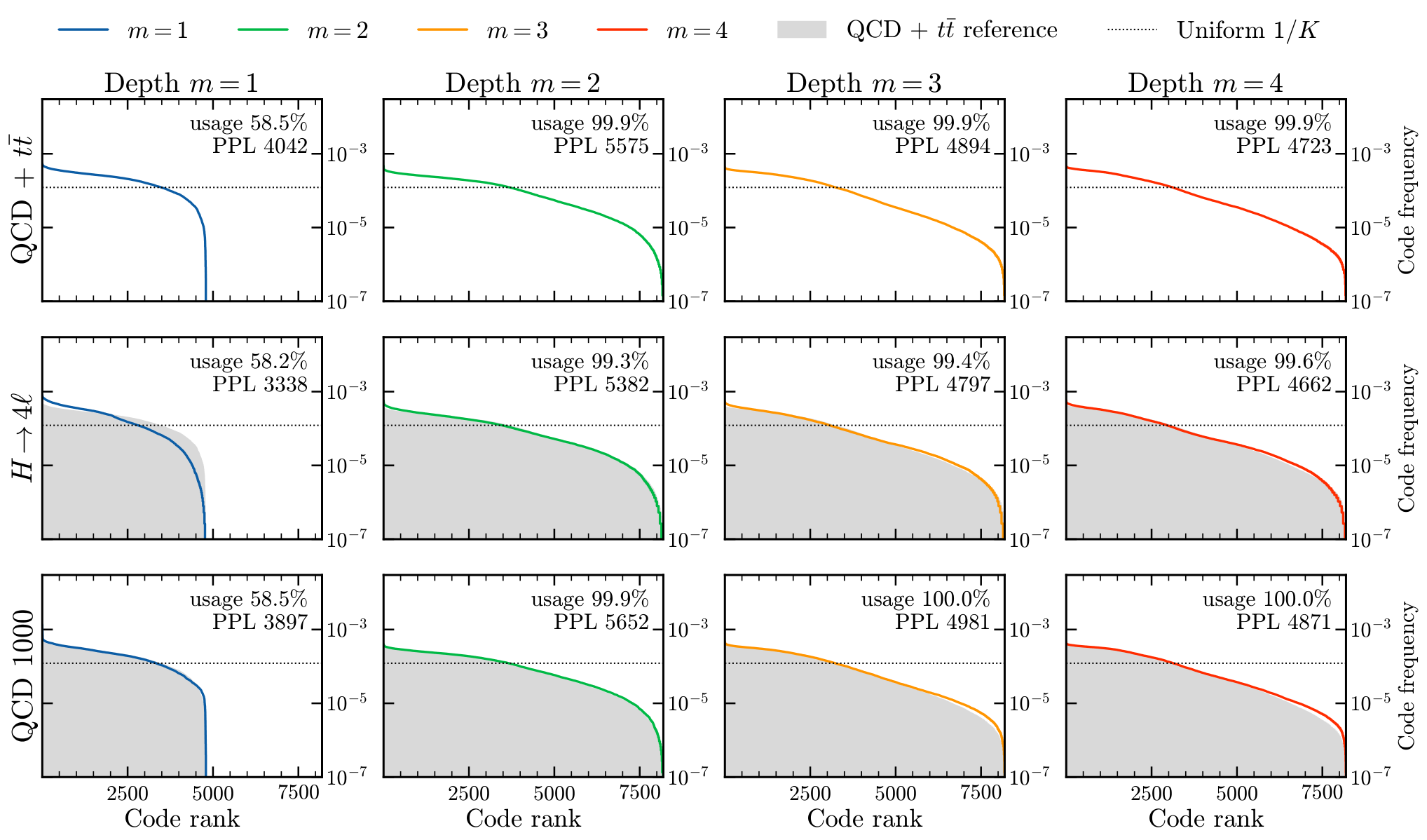
D.2 Generation results

We present the marginal feature distribution corresponding to the residual distributions presented in Section III.2. The spectra of particle features are available in Figure 10, those of jets in Figure 11, and finally the distributions of event-level features are shown in Figure 12. A comparison of the generation performance of different ablations is available in Table 10

Figure 10: Spectra of particle-level features for all three testing datasets. All histograms are normalized to unity; rows correspond to different datasets/processes while columns correspond to different observables.

Figure 11: Spectra of jet-level features for all three testing datasets. All histograms are normalized to unity; rows correspond to different datasets/processes while columns correspond to different observables.

Figure 12: Spectra of event-level features for all three testing datasets. All histograms are normalized to unity; rows correspond to different datasets/processes while columns correspond to different observables.

Table 10: Per-feature

W_{1}

distance between the FS and PF residual distributions, in the units of each feature, for the models trained on the full dataset for

4

epochs, on the held-out in-distribution test set (

50{,}000

events). The RQ-VAE column is the tokenizer reconstruction of an independent

50{,}000

-event sample with the same process mix, and the noise column the distance between two such independent PF samples. The best model in each row is in bold.

Event residuals
Residual	Unit	10M	22M	41M	97M	187M	1B	RQ-VAE	Noise
$\Delta H_{T}/H_{T}$	–	0.0212	0.0154	0.0102	0.00538	0.00526	0.00262	0.00144	0.00132
$\Delta E_{x}^{\mathrm{miss}}$	GeV	17.3	9.98	6.69	3.81	2.97	1.81	0.363	0.271
$\Delta E_{y}^{\mathrm{miss}}$	GeV	17.1	10.3	6.82	3.77	3.09	1.79	0.251	0.347
$\Delta E_{T}^{\mathrm{miss}}$	GeV	22.9	13.2	8.60	4.62	3.78	2.09	0.439	0.491
$\Delta N/N$	–	0.0195	0.0131	0.00940	0.0130	0.00629	0.00513	0.00793	0.00509
$\Delta N_{\mathrm{jets}}$	–	0.232	0.144	0.101	0.0646	0.0541	0.0292	0.00656	0.00612
Jet residuals
$\Delta p_{T}/p_{T}$	–	0.0708	0.0475	0.0344	0.0212	0.0171	0.00990	0.000811	0.000869
$\Delta\eta$	–	0.0306	0.0208	0.0152	0.0112	0.00994	0.00787	0.00296	0.000114
$\Delta\phi$	rad	0.0117	0.00783	0.00609	0.00424	0.00364	0.00248	0.000470	0.000105
$\Delta C_{2}$	–	0.00792	0.00504	0.00382	0.00237	0.00207	0.00127	0.000612	0.000198
$\Delta D_{2}$	–	0.433	0.327	0.271	0.240	0.218	0.189	0.135	0.0112
Particle residuals
$\Delta p_{T}/p_{T}$	–	1.12	0.813	0.670	0.526	0.477	0.392	0.212	0.00564
$\Delta\eta$	–	0.0285	0.0189	0.0154	0.0113	0.0103	0.00809	0.00357	0.000163
$\Delta\phi$	rad	0.0185	0.0111	0.00946	0.00625	0.00555	0.00398	0.00183	0.000225
$\Delta v_{z}$	mm	0.375	0.232	0.245	0.160	0.229	0.187	0.0356	0.0138
$\Delta v_{x}$	mm	0.0292	0.0414	0.0461	0.0328	0.0449	0.0309	0.00145	0.00143
$\Delta v_{y}$	mm	0.0310	0.0429	0.0513	0.0349	0.0458	0.0287	0.00178	0.00250