Generative Modeling of Stochastic Dynamics for Long-Time Evolution
Abstract
Exact stochastic equations for non-equilibrium dynamics are rarely accessible. We show that the long-time evolution of stochastic dynamics can be predicted from configuration pairs at a fixed short time lag, without knowledge of the equation of motion. Generative diffusion models learn the finite-time transition kernel from these pairs, and iterating it propagates the dynamics far beyond the training lag. For two-dimensional Model B, the diffusive dynamics of a conserved order parameter, the learned kernels reproduce dynamic critical scaling and self-similar coarsening. Agreement with direct simulations persists on lattices twice the largest training size and for initial ensembles absent from training. For driven colloids in a periodic optical potential, ten minutes of measured trajectories suffice to predict the particle current and mean passage time over the next twenty minutes within experimental uncertainty. Short-time observations thus contain the information needed to predict emergent non-equilibrium dynamics at much longer times.
Introduction.—The dynamical properties of a system are encoded in the time evolution of fluctuations, transport, and emergent structures. Experiments and microscopic simulations provide time-resolved configurations, while the effective equations governing their evolution are often unknown. From a data-driven perspective, deep learning has produced emulators for weather forecasting [1], fluid dynamics [2], and molecular dynamics [3, 4, 5]. Deep generative models can also sample equilibrium ensembles [6], including Boltzmann distributions of lattice fields [7, 8, 9, 10, 11, 12, 13, 14]. These approaches largely target deterministic evolution or static ensembles. In a fluctuating system, thermal noise is part of the dynamical law and shapes both relaxation and observable correlations. For systems with a few degrees of freedom, generative models can learn stochastic evolution from paired observations [15, 16]. Langevin inference instead assumes a Langevin equation and estimates its drift and diffusion from sampled trajectories [17, 18]. For an interacting field with many degrees of freedom, it remains open whether the dynamics and its emergent behavior can be reconstructed without assuming the form of the equation of motion.
For autonomous dynamics, this reconstruction can be formulated in terms of a transition kernel at a fixed, finite lag . The same kernel applies at every , and its -fold composition gives the exact transition law over . Here we learn this transition kernel from configuration pairs separated by using a conditional diffusion model (DM) [19, 20, 21]. Conditioned on the present field, the model samples its stochastic increment over that interval, as illustrated in Fig. 1. The decisive test of a learned kernel is whether it reproduces the physics at long times and for initial ensembles and system sizes absent from training.


As the first stringent test, we take two-dimensional Model B [23] of the Hohenberg–Halperin classification. It provides a diffusive description of critical relaxation and phase separation in binary alloys [24] and fluid mixtures [25], and of net-baryon fluctuations in relativistic heavy-ion collisions [26]. The conservation law slows the critical dynamics to [27, 28] and concentrates the difficulty in the longest wavelengths. It also freezes the spatial mean, , for every realization of the noise. In training, the generative model receives only the paired fields, no prior knowledge of the equation of motion or the equilibrium weight.
The learned kernels predict the dynamics over times up to , with each kernel trained at a single lag . The critical scaling analysis gives an effective dynamic exponent , against from direct integration. Relaxation times also agree with direct integration on a larger lattice excluded from training. Deep in the broken phase, a kernel trained on lattices up to generates phase separation on from a disordered start. The domain size follows the growth law of phase ordering [25] and stays within about two percent of the direct dynamics. These scaling laws are consequences of the equation of motion, and none of them can be read off the training pairs directly. Any autonomous stochastic dynamics that can be sampled in pairs, in an experiment or in a microscopic simulation, defines the same learning problem. A system with an explicit drive or with correlated noise can often be brought into this class by enlarging the set of dynamical variables. Applied to measured trajectories of driven colloids in a periodic optical potential [29], the same construction predicts the particle current and mean passage time within experimental uncertainty (End Matter).
Transition kernel.—Consider a field evolving under an autonomous stochastic equation of motion
| (1) |
where denotes the stochastic noise. Neither nor the probability law of depends on the choice of time origin. Equivalently, the noise path measure is invariant under a common translation of all time arguments. For a general time interval and an initial configuration , let denote a realization of the stochastic driving over . For fixed , the solution of Eq. 1 defines the pathwise increment
| (2) |
where is the trajectory generated by the driving history . Averaging over these histories gives the finite-time transition kernel
| (3) |
Thus specifies the update for a fixed noise history, and describes the distribution of possible updates. We learn from paired observations at the fixed training lag .
For simplicity, we begin with temporally white noise. The driving histories in Eq. 2 are then independent over successive intervals, so is a Markov state. Together with autonomy, this makes the transition law depend only on the interval, not on the origin. Composing the exact kernel therefore propagates the dynamics over arbitrarily long times, whereas a learned kernel must be tested for accumulated errors. Neither nor depends on the initial ensemble. The distinction between equilibrium fluctuations and non-equilibrium relaxation therefore enters through the distribution of initial states, rather than through the transition kernel itself. The construction is not restricted to white noise. Colored noise can be represented by additional dynamical variables driven by white noise, which enlarges the state but leaves the method unchanged. A pathwise derivation and the extension to colored noise are given in Sec. S1.
Conditional diffusion model.—Training data consist of pairs sampled from the underlying dynamics at a fixed lag . Taking the present configuration as the condition, the model learns the conditional distribution of the increment ,
| (4) |
Unlike standard regression, which predicts only the conditional mean, represents the fluctuations that determine equal-time and temporal correlations. We use a score-based diffusion model trained on and conditioned on . Repeated draws at fixed produce distinct increments corresponding to different stochastic realizations. The forward diffusion, score-matching objective, and reverse sampling construction are given in Sec. S2.
During training, the model receives only paired fields, without access to the underlying drift, noise statistics, or equilibrium weight. The input therefore has the same form as paired configurations obtained from experiments or molecular dynamics simulations. The training conditions and their coverage of field space are detailed in Sec. S3.
A sampled increment advances the field by the training lag ,
| (5) |
Iterating Eq. 5 composes the learned kernel by the Chapman–Kolmogorov composition and generates trajectories far beyond the training lag, as illustrated in Fig. 1. We next test this construction on models of dynamic critical behavior where universal scaling provides a stringent long-time benchmark.
Models of dynamic critical behavior.—Following Hohenberg and Halperin [23], dynamic critical behavior is governed by the relevant slow fields . These include the order parameter, conserved densities, and hydrodynamic variables associated with broken continuous symmetries. Their long-wavelength components relax slowly, while the remaining microscopic degrees of freedom equilibrate rapidly and enter through kinetic coefficients and stochastic forces. The coarse-grained evolution takes the general Langevin form
| (6) |
where and is the static free-energy functional. gives the fluctuation–dissipation relation. The kinetic operator governs dissipative relaxation and transport. In the simplest diagonal case with constant , describes local relaxation of nonconserved fields, while describes conserved transport. For conserved fields, the reversible term and noise must also take the form of current divergences.
The reversible term contains mode couplings generated by the Poisson brackets of the slow variables,
| (7) |
and does not contribute to entropy production. Equations (6) and (7) make stationary. Thus determines the statics, whereas the dynamics also depends on the slow fields, the kinetic operator , and the mode couplings .
These ingredients define the dynamic universality classes. Models A and B [28] contain only a nonconserved or conserved order parameter, respectively, with . Models C and D [27] couple the order parameter dissipatively to a conserved scalar density. Models E, F, G, H, and J [30, 31, 32] have , corresponding to reversible couplings involving conserved densities, symmetry generators, or transverse momentum. Systems in the same static universality class may therefore relax with different dynamic critical exponents, . For autonomous Markovian models, the kernel is conditioned on the complete set of slow fields.
For scalar Model B, we take , , and a continuum free energy . For periodic or no-flux boundaries, the mean field
| (8) |
is fixed for every noise realization, while the nonzero modes relax. We enforce conservation by projecting each generated increment onto the zero-mean subspace, preserving to floating-point accuracy. The lattice realization and implementation details are given in Sec. S3.
Trained on pairs generated from synthetic correlated Gaussian fields, the kernel reproduces long-time evolution from equilibrium and non-equilibrium initial ensembles absent from training. Fig. 2 compares its predictions at with direct integration using the stability-optimized stochastic Runge–Kutta scheme SOSRA [22]. The comparison includes an equilibrium hybrid Monte Carlo (HMC) ensemble [33] and an uncorrelated Gaussian ensemble far from equilibrium. For each ensemble, the learned and reference dynamics started from the same fields and were evolved to . For the diagonal modes , the equal-time power is , where and . The generated configurations reproduced the large-scale structure of the reference dynamics, while tracked the direct result both in equilibrium and during relaxation from the Gaussian ensemble. The mean field remained conserved to single-precision accuracy. Temporal correlations of the first four diagonal modes agreed with direct integration over the resolved range of time separations (Fig. S2). Details of the predictions are given in Sec. S4.
Critical relaxation and coarsening.—We characterize relaxation by the normalized correlation
| (9) |
where is the time separation and averages over trajectories and all time origins with that separation. On trajectories generated with a fixed lag , the available separations are with . We define by . At the critical point, dynamic scaling predicts
| (10) |
where is the lattice momentum magnitude at , with and .
The critical scaling analysis in Fig. 3 uses kernels trained on equilibrium pairs at , with training lags and to resolve the fast and slow modes. The learned and direct correlations approximately collapse onto the same nonexponential profile, with slower decay than at large . We describe this profile by
| (11) |
Its effective decay rate decreases from toward . We constrain the initial rate using the static fluctuations and the equilibrium fluctuation-dissipation relation (Sec. S4.3). Reproducing this crossover tests the learned dynamics beyond the critical exponent.
Fits to the relaxation times yield effective exponents for the learned kernels and for SOSRA, consistent within the quoted uncertainties. These values characterize the resolved momentum range; the asymptotic two-dimensional value is (Sec. S5).
The same equilibrium-trained kernels were then applied at the larger size . Across the resolved momentum range, the learned relaxation times agreed with the direct results, yielding for the learned kernel and for the direct dynamics (Fig. S5).
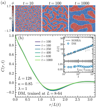
Deep in the broken phase, a separate kernel trained on synthetic domain fields at was applied at from a disordered initial state. The resulting fields underwent phase separation. Domain growth was quantified by the equal-time correlation of the sign field [34],
| (12) |
where the average is over lattice sites, orientations of , and trajectories. Because , without further normalization. The domain size is defined as the first zero of [35]. For a conserved scalar order parameter, phase-ordering scaling predicts [36, 37, 38, 25]
| (13) |
Between and , correlations from the learned dynamics collapsed onto a single scaling curve (Fig. 4). The corresponding domain size followed the growth law and remained within about two percent of the direct Model B result. The structure factor also exhibited the Porod scaling expected for sharp domain walls [39, 25] (Sec. S4).
Discussion.—The dynamic exponent and coarsening law are collective consequences of the dynamics, but neither is imposed during training. Each kernel is learned from configuration pairs at a fixed lag, of the kind obtainable from experiments or microscopic simulations, without long-time trajectories or scaling observables as training targets. Recovering these laws through repeated application of the learned kernels provides a nontrivial test of their ability to reproduce long-time collective dynamics.
The same construction can be used whenever the measured variables form a sufficient state. A reconstruction from trajectories of driven colloids in a periodic optical potential is reported in the End Matter [29]. Beyond the training window, the learned kernel reproduces the measured particle current and mean passage time under driving to within , whereas a Langevin reference based on Ref. [29] deviates by about .
The same construction can be extended to systems with memory by including suitable auxiliary variables in the state [40]. Active and reaction–diffusion systems may require additional slow fields in the conditioned state [41, 42]. Periodic drives can be included through the drive phase [43]. The construction may also be extended to other Hohenberg–Halperin classes. Model A describes local relaxation of a nonconserved order parameter [28, 44, 45]. Model H couples a conserved order parameter to conserved momentum through reversible terms [46, 47, 48]. The resulting interplay of diffusion and advection governs critical relaxation in fluids and at the critical end point of quantum chromodynamics [23, 49]. Beyond critical phenomena, the same approach could be applied to stochastic hydrodynamics and molecular dynamics.
Conclusions.—Finite-time transition kernels can be learned from paired observations and iterated without an explicit equation of motion. In Model B, this reconstruction recovered critical relaxation, transfer to a larger lattice, and phase ordering far beyond the training lag. Trained on experimental trajectories of driven colloids, it predicted the particle current and mean passage time within experimental uncertainty, more accurately than a Langevin reference. How far this extends depends on which slow variables a pair of observations has to carry, and that choice differs for every dynamic universality class.
Acknowledgments.— We thank Gert Aarts, Yuto Ashida, Kenji Fukushima, Satoshi Iso, Jan M. Pawlowski and other DM-QFT collaboration members for insightful discussions. We thank the DEEP-IN working group at RIKEN-iTHEMS for support in the preparation of this paper. This research is partially supported by Initiative on Recommendation Program for Young Researchers and Woman Researchers, Information Technology Center, The University of Tokyo. We also thank the support from Google DeepMind team. LW and YT are supported by the JST-BOOST Grant No. JPMJBY24H9. LW is also supported by the RIKEN-TRIP initiative (RIKEN-Quantum) and JSPS KAKENHI Grant No. 25H01560.
Code availability.—The code used in this work will be made publicly available upon publication.
Use of AI tools.—GPT 6 Astra (OpenAI) and Claude Fable 5 (Anthropic) assisted substantially with numerical cross-checks and with polishing the manuscript. All derivations, results, and statements were verified by authors, who take full responsibility for the content.
References
- [1] R. Lam, A. Sanchez-Gonzalez, M. Willson, P. Wirnsberger, M. Fortunato, F. Alet, S. Ravuri, T. Ewalds, Z. Eaton-Rosen, W. Hu, A. Merose, S. Hoyer, G. Holland, O. Vinyals, J. Stott, A. Pritzel, S. Mohamed, and P. Battaglia, Learning skillful medium-range global weather forecasting, Science 382, 1416 (2023).
- [2] D. Kochkov, J. A. Smith, A. Alieva, Q. Wang, M. P. Brenner, and S. Hoyer, Machine learning-accelerated computational fluid dynamics, Proc. Natl. Acad. Sci. U.S.A. 118, e2101784118 (2021).
- [3] L. Klein, A. Y. K. Foong, T. E. Fjelde, B. Mlodozeniec, M. Brockschmidt, S. Nowozin, F. Noé, and R. Tomioka, Timewarp: Transferable acceleration of molecular dynamics by learning time-coarsened dynamics, in Advances in Neural Information Processing Systems, Vol. 36 (2023) pp. 52863–52883, arXiv:2302.01170 [stat.ML] .
- [4] F. Bigi, J. Spies, and M. Ceriotti, Learning the action for long-time-step simulations of molecular dynamics, Phys. Rev. Lett. 136, 237301 (2026), arXiv:2508.01068 [physics.chem-ph] .
- [5] N. Shoghi, Y. Liu, Y. Shen, R. Brekelmans, P. Li, and Q. Gu, Scalable spatio-temporal SE(3) diffusion for long-horizon protein dynamics, in International Conference on Learning Representations (2026) arXiv:2602.02128 [cs.LG] .
- [6] F. Noé, S. Olsson, J. Köhler, and H. Wu, Boltzmann generators: Sampling equilibrium states of many-body systems with deep learning, Science 365, eaaw1147 (2019).
- [7] J. M. Pawlowski and J. M. Urban, Reducing Autocorrelation Times in Lattice Simulations with Generative Adversarial Networks, Mach. Learn. Sci. Tech. 1, 045011 (2020), arXiv:1811.03533 [hep-lat] .
- [8] M. S. Albergo, G. Kanwar, and P. E. Shanahan, Flow-based generative models for Markov chain Monte Carlo in lattice field theory, Phys. Rev. D 100, 034515 (2019).
- [9] K. A. Nicoli, C. J. Anders, L. Funcke, T. Hartung, K. Jansen, P. Kessel, S. Nakajima, and P. Stornati, Estimation of Thermodynamic Observables in Lattice Field Theories with Deep Generative Models, Phys. Rev. Lett. 126, 032001 (2021), arXiv:2007.07115 [hep-lat] .
- [10] K. Cranmer, G. Kanwar, S. Racanière, D. J. Rezende, and P. E. Shanahan, Advances in machine-learning-based sampling motivated by lattice quantum chromodynamics, Nature Rev. Phys. 5, 526 (2023), arXiv:2309.01156 [hep-lat] .
- [11] L. Wang, G. Aarts, and K. Zhou, Diffusion models as stochastic quantization in lattice field theory, JHEP 2024 (05), 060, arXiv:2309.17082 [hep-lat] .
- [12] G. Aarts, D. E. Habibi, L. Wang, and K. Zhou, On learning higher-order cumulants in diffusion models, Mach. Learn. Sci. Tech. 6, 025004 (2025), arXiv:2410.21212 [hep-lat] .
- [13] Q. Zhu, G. Aarts, W. Wang, K. Zhou, and L. Wang, Physics-conditioned diffusion models for lattice gauge theory, JHEP 2026 (03), 111, arXiv:2502.05504 [hep-lat] .
- [14] G. Aarts, D. E. Habibi, A. Ipp, D. I. Müller, T. R. Ranner, L. Wang, W. Wang, and Q. Zhu, Generalizable Equivariant Diffusion Models for Non-Abelian Lattice Gauge Theory (2026), arXiv:2601.19552 [hep-lat] .
- [15] Y. Chen and D. Xiu, Learning stochastic dynamical system via flow map operator, J. Comput. Phys. 508, 112984 (2024), arXiv:2305.03874 [cs.LG] .
- [16] Y. Liu, Y. Chen, D. Xiu, and G. Zhang, A training-free conditional diffusion model for learning stochastic dynamical systems, SIAM J. Sci. Comput. 47, C1144 (2025), arXiv:2410.03108 [cs.LG] .
- [17] A. Frishman and P. Ronceray, Learning force fields from stochastic trajectories, Phys. Rev. X 10, 021009 (2020).
- [18] D. B. Brückner, P. Ronceray, and C. P. Broedersz, Inferring the dynamics of underdamped stochastic systems, Phys. Rev. Lett. 125, 058103 (2020).
- [19] Y. Song and S. Ermon, Generative modeling by estimating gradients of the data distribution, in Advances in Neural Information Processing Systems, Vol. 32 (2019) arXiv:1907.05600 [cs.LG] .
- [20] J. Ho, A. Jain, and P. Abbeel, Denoising diffusion probabilistic models, in Advances in Neural Information Processing Systems, Vol. 33 (2020) pp. 6840–6851, arXiv:2006.11239 [cs.LG] .
- [21] Y. Song, J. Sohl-Dickstein, D. P. Kingma, A. Kumar, S. Ermon, and B. Poole, Score-based generative modeling through stochastic differential equations, in International Conference on Learning Representations (2021) arXiv:2011.13456 [cs.LG] .
- [22] C. Rackauckas and Q. Nie, Stability-optimized high order methods and stiffness detection for pathwise stiff stochastic differential equations, in 2020 IEEE High Performance Extreme Computing Conference (HPEC) (2020) pp. 1–8, arXiv:1804.04344 [math.NA] .
- [23] P. C. Hohenberg and B. I. Halperin, Theory of Dynamic Critical Phenomena, Rev. Mod. Phys. 49, 435 (1977).
- [24] J. W. Cahn, On spinodal decomposition, Acta Metall. 9, 795 (1961).
- [25] A. J. Bray, Theory of phase-ordering kinetics, Adv. Phys. 43, 357 (1994), arXiv:cond-mat/9501089 .
- [26] M. Nahrgang, M. Bluhm, T. Schaefer, and S. A. Bass, Diffusive dynamics of critical fluctuations near the QCD critical point, Phys. Rev. D 99, 116015 (2019), arXiv:1804.05728 [nucl-th] .
- [27] B. I. Halperin, P. C. Hohenberg, and S.-k. Ma, Renormalization-group methods for critical dynamics: I. Recursion relations and effects of energy conservation, Phys. Rev. B 10, 139 (1974).
- [28] B. I. Halperin, P. C. Hohenberg, and S.-k. Ma, Renormalization-group methods for critical dynamics: II. Detailed analysis of the relaxational models, Phys. Rev. B 13, 4119 (1976a).
- [29] C. Dieball, Y. Mohebi Satalsari, A. B. Zuccolotto-Bernez, S. U. Egelhaaf, M. A. Escobedo-Sánchez, and A. Godec, Precisely controlled colloids: a playground for path-wise non-equilibrium physics, Soft Matter 21, 2170 (2025).
- [30] B. I. Halperin, P. C. Hohenberg, and E. D. Siggia, Renormalization-group treatment of the critical dynamics of superfluid helium, the isotropic antiferromagnet, and the easy-plane ferromagnet, Phys. Rev. B 13, 1299 (1976b).
- [31] E. D. Siggia, B. I. Halperin, and P. C. Hohenberg, Renormalization-group treatment of the critical dynamics of the binary-fluid and gas-liquid transitions, Phys. Rev. B 13, 2110 (1976).
- [32] S.-k. Ma and G. F. Mazenko, Critical dynamics of ferromagnets in dimensions: General discussion and detailed calculation, Phys. Rev. B 11, 4077 (1975).
- [33] S. Duane, A. D. Kennedy, B. J. Pendleton, and D. Roweth, Hybrid Monte Carlo, Phys. Lett. B 195, 216 (1987).
- [34] S. Puri, A. J. Bray, and J. L. Lebowitz, Phase-separation kinetics in a model with order-parameter-dependent mobility, Phys. Rev. E 56, 758 (1997).
- [35] J. Zhu, L.-Q. Chen, J. Shen, and V. Tikare, Coarsening kinetics from a variable-mobility Cahn-Hilliard equation: Application of a semi-implicit Fourier spectral method, Phys. Rev. E 60, 3564 (1999).
- [36] I. M. Lifshitz and V. V. Slyozov, The kinetics of precipitation from supersaturated solid solutions, J. Phys. Chem. Solids 19, 35 (1961).
- [37] D. A. Huse, Corrections to late-stage behavior in spinodal decomposition: Lifshitz-Slyozov scaling and Monte Carlo simulations, Phys. Rev. B 34, 7845 (1986).
- [38] T. M. Rogers, K. R. Elder, and R. C. Desai, Numerical study of the late stages of spinodal decomposition, Phys. Rev. B 37, 9638 (1988).
- [39] G. Porod, Die Röntgenkleinwinkelstreuung von dichtgepackten kolloiden Systemen. I. Teil, Kolloid-Z. 124, 83 (1951).
- [40] H. Mori, Transport, Collective Motion, and Brownian Motion, Prog. Theor. Phys. 33, 423 (1965).
- [41] J. Toner and Y. Tu, Long-range order in a two-dimensional dynamical model: How birds fly together, Phys. Rev. Lett. 75, 4326 (1995).
- [42] A. M. Turing, The chemical basis of morphogenesis, Philos. Trans. R. Soc. Lond. B 237, 37 (1952).
- [43] G. Froyland and P. Koltai, Estimating long-term behavior of periodically driven flows without trajectory integration, Nonlinearity 30, 1948 (2017).
- [44] Y.-y. Tan, S. Yin, Y.-r. Chen, C. Huang, and W.-j. Fu, Real-time evolution of critical modes in the QCD phase diagram, Phys. Rev. D 114, L011501 (2026a), arXiv:2512.03614 [hep-ph] .
- [45] Y.-y. Tan, Y.-r. Chen, W.-j. Fu, and W.-J. Li, Universality of pseudo-Goldstone damping near critical points, Nature Commun. 16, 2916 (2025), arXiv:2403.03503 [hep-th] .
- [46] Y.-r. Chen, Y.-y. Tan, and W.-j. Fu, Critical dynamics of model H within the real-time FRG approach, Phys. Rev. D 111, 094025 (2025), arXiv:2406.00679 [hep-ph] .
- [47] J. V. Roth, Y. Ye, S. Schlichting, and L. von Smekal, Universal critical dynamics near the chiral phase transition and the QCD critical point, Phys. Rev. D 111, L111901 (2025), arXiv:2409.14470 [hep-ph] .
- [48] C. Chattopadhyay, J. Ott, T. Schaefer, and V. V. Skokov, Simulations of Stochastic Fluid Dynamics near a Critical Point in the Phase Diagram, Phys. Rev. Lett. 133, 032301 (2024), arXiv:2403.10608 [nucl-th] .
- [49] D. T. Son and M. A. Stephanov, Dynamic universality class of the QCD critical point, Phys. Rev. D 70, 056001 (2004), arXiv:hep-ph/0401052 .
- [50] C. Dieball, Y. Mohebi Satalsari, A. B. Zuccolotto-Bernez, S. U. Egelhaaf, M. A. Escobedo-Sánchez, and A. Godec, Dataset for “Precisely controlled colloids: a playground for path-wise non-equilibrium physics”, Zenodo (2024).
- [51] C. Rackauckas and Q. Nie, DifferentialEquations.jl – a performant and feature-rich ecosystem for solving differential equations in Julia, J. Open Res. Softw. 5, 15 (2017).
- [52] J. M. Foster, G. dos Reis, and C. Strange, High order splitting methods for SDEs satisfying a commutativity condition, SIAM J. Numer. Anal. 62, 500 (2024).
- [53] P. Kidger, On Neural Differential Equations, Ph.D. thesis, University of Oxford (2021), arXiv:2202.02435 [cs.LG] .
- [54] G. Maruyama, Continuous Markov processes and stochastic equations, Rend. Circ. Mat. Palermo 4, 48 (1955).
- [55] P. Vincent, A connection between score matching and denoising autoencoders, Neural Comput. 23, 1661 (2011).
- [56] B. D. O. Anderson, Reverse-time diffusion equation models, Stoch. Process. Appl. 12, 313 (1982).
- [57] G. Parisi and Y.-s. Wu, Perturbation Theory Without Gauge Fixing, Sci. Sin. 24, 483 (1981).
- [58] P. H. Damgaard and H. Hüffel, Stochastic Quantization, Phys. Rept. 152, 227 (1987).
- [59] K. Fukushima and S. Kamata, Stochastic Quantization and Diffusion Models, J. Phys. Soc. Jap. 94, 031010 (2025), arXiv:2411.11297 [hep-lat] .
- [60] Y. Hirono, A. Tanaka, and K. Fukushima, Understanding Diffusion Models by Feynman’s Path Integral (2024), arXiv:2403.11262 [cs.LG] .
- [61] L. Wang, Stochastic Quantization as Optimal Control (2026), arXiv:2607.21436 [hep-lat] .
- [62] F. Ihssen and J. M. Pawlowski, Physics-informed renormalisation group flows, Annals Phys. 481, 170177 (2025), arXiv:2409.13679 [hep-th] .
- [63] M. Bauer, R. Kapust, J. M. Pawlowski, and F. L. Temmen, Super-resolving normalising flows for lattice field theories, SciPost Phys. 19, 077 (2025), arXiv:2412.12842 [hep-lat] .
- [64] K. Masuki and Y. Ashida, Generative diffusion model with inverse renormalization group flows (2025), arXiv:2501.09064 [cond-mat.stat-mech] .
- [65] K. Masuki and Y. Ashida, Renormalization Group Flow Matching for Scalable Local Generative Modeling (2026), arXiv:2608.23696 [cs.LG] .
- [66] Y.-y. Tan, G. Aarts, D. E. Habibi, B. Lucini, and L. Wang, Diffusion Models for Sampling Near Criticality in Lattice Field Theories (2026b), arXiv:2607.08505 [hep-lat] .
- [67] D. Schweitzer, S. Schlichting, and L. von Smekal, Critical dynamics of relativistic diffusion, Nucl. Phys. B 984, 115944 (2022), arXiv:2110.01696 [hep-lat] .
- [68] J. V. Roth and L. von Smekal, Critical dynamics in a real-time formulation of the functional renormalization group, JHEP 2023 (10), 065.
- [69] K. Kawasaki, Diffusion constants near the critical point for time-dependent Ising models. I, Phys. Rev. 145, 224 (1966).
- [70] W. Zhong, D. Panja, and G. T. Barkema, Approximate dynamical eigenmodes of the Ising model with local spin-exchange moves, Phys. Rev. E 100, 012132 (2019).
- [71] C. Chattopadhyay, J. Ott, T. Schaefer, and V. Skokov, Dynamic scaling of order parameter fluctuations in model B, Phys. Rev. D 108, 074004 (2023), arXiv:2304.07279 [nucl-th] .
- [72] K. Binder and D. Stauffer, Theory for the slowing down of the relaxation and spinodal decomposition of binary mixtures, Phys. Rev. Lett. 33, 1006 (1974).
- [73] H. Furukawa, A dynamic scaling assumption for phase separation, Adv. Phys. 34, 703 (1985).
- [74] P. Debye, H. R. Anderson, and H. Brumberger, Scattering by an inhomogeneous solid. II. The correlation function and its application, J. Appl. Phys. 28, 679 (1957).
- [75] J. G. Amar, F. E. Sullivan, and R. D. Mountain, Monte Carlo study of growth in the two-dimensional spin-exchange kinetic Ising model, Phys. Rev. B 37, 196 (1988).
- [76] S. Puri and Y. Oono, Study of phase-separation dynamics by use of cell dynamical systems. II. Two-dimensional demonstrations, Phys. Rev. A 38, 1542 (1988).
- [77] B. König, O. J. J. Ronsin, and J. Harting, Two-dimensional Cahn–Hilliard simulations for coarsening kinetics of spinodal decomposition in binary mixtures, Phys. Chem. Chem. Phys. 23, 24823 (2021).
- [78] J. U. Garcia, D. R. Tree, A. Bagoyo, T. Iwama, K. T. Delaney, and G. H. Fredrickson, Coarsening dynamics of ternary polymer solutions with mobility and viscosity contrasts, J. Chem. Phys. 159, 214904 (2023).
- [79] G. Krausch, C.-A. Dai, E. J. Kramer, and F. S. Bates, Real space observation of dynamic scaling in a critical polymer mixture, Phys. Rev. Lett. 71, 3669 (1993).
- [80] A. Zhiliakov, Y. Wang, A. Quaini, M. Olshanskii, and S. Majd, Experimental validation of a phase-field model to predict coarsening dynamics of lipid domains in multicomponent membranes, Biochim. Biophys. Acta Biomembr. 1863, 183446 (2021).
- [81] D. P. Arnold, A. Gubbala, and S. C. Takatori, Active surface flows accelerate the coarsening of lipid membrane domains, Phys. Rev. Lett. 131, 128402 (2023).
- [82] M. M. C. Tortora, L. D. Brennan, G. Karpen, and D. Jost, HP1-driven phase separation recapitulates the thermodynamics and kinetics of heterochromatin condensate formation, Proc. Natl. Acad. Sci. U.S.A. 120, e2211855120 (2023).
- [83] T. Karras, M. Aittala, T. Aila, and S. Laine, Elucidating the design space of diffusion-based generative models, in Advances in Neural Information Processing Systems, Vol. 35 (2022) pp. 26565–26577, arXiv:2206.00364 [cs.LG] .
- [84] K. Zheng, C. Lu, J. Chen, and J. Zhu, DPM-Solver-v3: Improved diffusion ODE solver with empirical model statistics, in Advances in Neural Information Processing Systems, Vol. 36 (2023) pp. 55502–55542, arXiv:2310.13268 [cs.CV] .
- [85] C. Lu, Y. Zhou, F. Bao, J. Chen, C. Li, and J. Zhu, DPM-Solver: A fast ODE solver for diffusion probabilistic model sampling in around 10 steps, in Advances in Neural Information Processing Systems, Vol. 35 (2022) pp. 5775–5787, arXiv:2206.00927 [cs.LG] .
- [86] C. Lu, Y. Zhou, F. Bao, J. Chen, C. Li, and J. Zhu, DPM-Solver++: Fast solver for guided sampling of diffusion probabilistic models, Mach. Intell. Res. 22, 730 (2025), arXiv:2211.01095 [cs.LG] .
- [87] M. C. Yalabik and J. D. Gunton, Monte Carlo renormalization-group studies of kinetic Ising models, Phys. Rev. B 25, 534(R) (1982).
- [88] L. L. Moseley, P. W. Gibbs, and N. Jan, Dynamic Monte Carlo renormalization group. II, J. Stat. Phys. 57, 421 (1989).
- [89] B. Zheng, Monte Carlo simulations of critical dynamics with conserved order parameter, Phys. Lett. A 277, 257 (2000).
- [90] B. Zheng, Erratum to “Monte Carlo simulations of critical dynamics with conserved order parameter”, Phys. Lett. A 282, 132 (2001).
- [91] X. Li, T.-K. L. Wong, R. T. Q. Chen, and D. Duvenaud, Scalable gradients for stochastic differential equations, in Proceedings of the Twenty Third International Conference on Artificial Intelligence and Statistics, Proceedings of Machine Learning Research, Vol. 108 (PMLR, 2020) pp. 3870–3882.
End Matter
Computational cost. We benchmark the learned kernel against leading publicly available stochastic solvers on the same NVIDIA GH200 GPU (Table 1). For the same ensembles and evolution time at comparable accuracy, the learned kernel is faster than every public implementation tested. Our fused SOSRA implementation is faster in equilibrium and comparable in cost out of equilibrium.
Colloid experiment. We apply our framework to an experiment on colloidal particles in a periodic potential [29, 50]. The particles diffuse in a quasi-two-dimensional cell subject to a periodic optical potential along . In the absence of external driving, thermal fluctuations produce motion within individual wells together with activated hopping between neighboring wells. Translating the sample cell relative to the optical pattern biases these hopping processes and generates a non-equilibrium particle current. The same system therefore probes both thermally activated transport and driven stochastic dynamics.
DM predictions for undriven (upper row) and driven (lower row) colloidal motion in a periodic potential [29, 50]. Black circles show the experimental data. Blue solid lines show DM and orange dashed lines the Langevin reference based on Ref. [29]. (a,e) Mean position . Shading shows the standard error of the mean displacement from . The dotted line at min marks the end of training. (b,f) Distributions of the net displacement over min of undriven motion and min of driven motion, both measured from min. (c,g) Mean displacement rate at s as a function of the initial phase . Gray dashed lines show the instantaneous Langevin drift , corresponding to . (d,h) Mean passage time conditioned on passage before . The target lies one potential period from the initial position, in either direction in (d) and along the drive in (h). Passage times are evaluated at s resolution. The gray line in (h) shows the continuous-time mean passage time, the period divided by the mean speed during training.
Separate kernels are learned for the undriven and driven dynamics from position pairs separated by s, conditioned on the particle’s phase within one period of the optical potential. Starting from the measured positions at min, the kernels are iterated to predict the subsequent min of undriven motion and min of driven motion.
DM retains the weak net drift in the undriven experiment [Fig. End Matter(a)], which the equilibrium Langevin reference based on Ref. [29] omits. This effect is learned from the measured motion without specifying its physical origin. Under driving, the predicted mean speed agrees with experiment to within [Fig. End Matter(e)].
DM also closely reproduces the measured displacement distributions [Fig. End Matter(b,f)] and passage-time statistics [Fig. End Matter(d,h)]. Its overall accuracy is comparable to that of the Langevin reference, with closer agreement for the driven mean current and mean passage time [Fig. End Matter(e,h)]. Further comparisons are given in Sec. S7.
| Wall time (s) | ||
|---|---|---|
| Method | Eq. | Noneq. |
| DPM-Solver-v3 (This work) | ||
| SOSRA (This work) | ||
| SOSRA (StochasticDiffEq.jl) [22, 51] | ||
| ShARK (Diffrax) [52, 53] | ||
| EM (Diffrax) [54, 53] | ||
| EM (other GPU/CPU solvers) [54] | ||
Supplemental Material for “Generative Modeling of Stochastic Dynamics for Long-Time Evolution”
S1 Finite-time composition and colored noise
The finite-time construction requires a state that determines the conditional law of future configurations. For the white-noise dynamics studied here, this state is .
Let and denote the driving histories over successive intervals of lengths and , expressed relative to the start of each interval. Their concatenation is . With the intermediate state , causality and uniqueness give
| (S1) | ||||
This identity holds for each realization before averaging over the driving. For a complete Markov state, the conditional law of the second update depends on the past only through . Autonomy makes that law independent of the time origin. Averaging the two successive updates therefore gives the Chapman–Kolmogorov identity
| (S2) |
Independent draws from the exact kernel , conditioned on the current state, thus reproduce the joint distribution of configurations at for any chosen initial ensemble. This result concerns the sampled times and does not specify the intervening trajectories. For a learned kernel, small errors in each update can accumulate over successive intervals. Agreement over one interval therefore does not guarantee accurate long-time dynamics. This must be tested by comparing observables from generated trajectories with measurements or direct simulations.
For colored noise, let denote the dynamical variables that carry its temporal correlations and use the joint state . When this state is autonomous and Markovian, its transition kernel obeys Eq. S2 with replaced by . The learning construction is unchanged, with training pairs . Each sampled update advances both the field and the noise variables, preserving the memory between successive physical intervals.
S2 Conditional diffusion construction

For each observed pair, the present state is the condition and is the target increment. Predicting an increment is convenient for slowly evolving fields, although the construction also applies to the next state itself. For coupled fields, contains all variables required for a Markov description.
To represent we diffuse only the increment and pass the condition to the score network as an unperturbed input. A variance-exploding (VE) process [21],
| (S3) |
with auxiliary diffusion time , noise , and , defines a family of noisy conditional distributions. The auxiliary time is distinct from the physical time and the fixed training lag . We train the score by denoising score matching [55],
| (S4) |
The average is over the measured pairs, the auxiliary time, and the added Gaussian noise. The objective contains neither the physical drift nor the physical noise covariance. The physical dynamics enters through the pairs.
One finite physical-time increment is drawn by integrating the conditional reverse-time SDE [56, 21],
| (S5) |
The equation is integrated from toward at fixed . Here denotes the Wiener process in this direction, with increment covariance . Sampling starts from a Gaussian whose variance is set by . This approximates the terminal forward distribution when the added noise dominates the target increment. The sampled increment is added to the condition according to Eq. 5. At the next physical step the condition is updated and a fresh history of the auxiliary noise is drawn. The reverse-time evolution is itself a Langevin process on configuration space whose drift is proportional to the learned score, in analogy with stochastic quantization [57, 58]. This correspondence has been developed for lattice field theories in [11, 59, 60]. Stochastic quantization has also been formulated as an optimal control problem at finite auxiliary time [61]. Renormalization group flows give a further reading of generative flows [62, 63, 64, 65].
S3 Numerical details of the Model B case study
S3.1 Lattice realization
For the conserved scalar field considered in the main text, Eq. 6 reduces to
| (S6) |
We use the lattice action
| (S7) |
on a periodic lattice with and unit spacing. Here is the hopping parameter, the dimensionless self-coupling, and a lattice unit vector.
Writing with Gaussian current noise , we define
| (S8) |
For periodic or no-flux boundaries, the net boundary flux vanishes. Integrating the continuity equation gives in every realization. We discretize the current with nearest-neighbor differences and use . We set throughout the Model B calculations. We use HMC to sample equilibrium initial fields with Boltzmann weight . Fig. S1 illustrates this local conservation law during phase ordering through the field change and the integrated total current.
Training targets are obtained by direct SOSRA integration with step size . For the Gaussian initial fields used to train the kernel in Fig. 2, the first unit of physical time uses step size before returning to . All generated pairs are used for training.
S3.2 Training pairs
The training data for the kernel used in Fig. 2 of the main text contain pairs at , generated from initial fields
| (S9) |
where . The mean-zero part is drawn from
| (S10) |
where is independent unit-variance Gaussian noise, , and . The three parameters are sampled independently. The initial field is evolved over the training lag , and the target is the resulting increment.
The training data for the kernels used in Figs. 3 and S5 are generated from canonical ensembles at , with initial fields at each size. No field is included in these training sets. Separate kernels are trained at and . The single-size kernel in Figs. S6 and S7 is trained on the canonical pairs alone.
The training data for the kernel used in Fig. 4 are generated from centered synthetic domain fields at . Let
| (S11) |
denote the projector onto zero-mean fields. The initial fields are
| (S12) |
where is a smoothed Gaussian field with correlation length . We draw independent unit-variance Gaussian noise , multiply each Fourier mode by , and set the mode to zero so that the spatial mean vanishes. The resulting real-space field is divided by its root-mean-square value , so that every sample has unit variance. The hyperbolic tangent then hardens the level sets of into domains of size with walls of width . The added noise is independent of . We sample , , , and . With probability , we instead set and draw . The target increment is obtained by evolving each synthetic field for the training lag . We generate pairs at each size.
Since the dynamics is symmetric under , the transition kernel satisfies , and every training pair is also used with both signs reversed.
S3.3 Score model and reverse sampling
The network operates on rescaled fields and , where and are the largest absolute values of the increment and of the initial field over the training set. For the VE process we use
| (S13) |
with . We use at and at . The score is represented by the modified NCSN++ network introduced in Ref. [66]. It uses periodic convolutions and omits the internal residual connections of NCSN++ [21], while retaining the encoder-to-decoder skip connections. Its inputs are the noisy increment, the initial field, and the auxiliary time. Training uses Adam with learning rate .
Sampling uses an exponential moving average of the network weights. The reverse process starts from and is integrated with 2000 Euler–Maruyama (EM) steps, logarithmically spaced in down to . Independent reverse noise is used for successive physical intervals.
Conservation is imposed only when drawing a transition, using the projector of Eq. S11. The initial Gaussian residual is projected with . At every reverse step, both the predicted score and the newly drawn Gaussian noise are projected with the same operator. The sampled process is therefore
| (S14) |
The final residual is rescaled to physical units and projected once more before it is added to the condition. Consequently for every generated transition and is preserved up to floating-point roundoff. The projection fixes only the zero mode and leaves the other modes to the learned dynamics.
The comparison with DPM-Solver-v3 is given in Sec. S5.
S4 Model B observables, critical relaxation, and coarsening
S4.1 Initial ensembles and statistical errors
For Fig. 2, we use equilibrium initial fields and uncorrelated Gaussian initial fields at . Each Gaussian field is shifted to have the same spatial mean as its paired equilibrium field, so that the conserved zero mode is matched between the two ensembles. DM and SOSRA start from the same initial configurations but use independent stochastic noise. Fig. 2 shows the evolution up to . All available time origins of the equilibrium trajectories are used to evaluate the correlations in Fig. S2.
For Fig. 3, the two DM kernels start from the same equilibrium initial fields at . The kernel is iterated to , and the kernel is iterated to . The SOSRA reference starts from the same initial fields and is evolved to in a single run. Configurations are recorded every up to and every thereafter, so that each learned kernel is compared with the reference dynamics on the corresponding time grid.
For Fig. 4, the kernel trained on synthetic domain fields at is applied at and . We use initial fields
| (S15) |
where is independent unit-variance Gaussian noise. Each field is evolved with to . The SOSRA reference uses independent trajectories initialized from the same distribution.
For each mode index , we average over the four symmetry-related wave vectors of . This average is performed separately for the equal-time quantity and the unequal-time product before constructing and . The bands and error bars of in Fig. 2 show standard errors over trajectories. For in Fig. S2, we estimate the uncertainty with a leave-one-trajectory-out jackknife. For each jackknife sample, the complete estimator in Eq. 9 is recomputed after removing one trajectory.
S4.2 Relaxation times and dynamic critical exponent
The relaxation time of each mode is extracted from the decay of with the time separation . Correlations are measured on two time grids with spacings and . The fine grid resolves the short-time decay up to , while the coarse grid extends the correlation to .
We obtain by linear interpolation between the two neighboring grid points that bracket the crossing. Dynamic critical scaling predicts , Eq. 10. We therefore extract the dynamic critical exponent from the unweighted fit
| (S16) |
At , the fit includes . At , we use , where the slowest mode is excluded because lies beyond the simulated time window.
Statistical uncertainties are estimated from bootstrap resamples of whole trajectories. For each dynamics, the same trajectory resample is used on both time grids, preserving their statistical correlation. Each bootstrap sample recomputes , , and . The quoted uncertainties are the standard deviations over the bootstrap ensemble.
S4.3 Dynamic scaling function
We fit Eq. 11 jointly to the four resolved modes in Fig. 3. The fits use the pointwise variances and do not include correlations between time separations.
Previous studies describe long-wavelength relaxation using near-Lorentzian critical spectra [67, 68], approximate dynamical eigenmodes of Kawasaki dynamics [69, 70], and exponential fits in three-dimensional Model B [71]. Eq. 11 allows an algebraic correction to an exponential tail, at large .
The short-time behavior is constrained independently by the equilibrium dynamics. For Model B, conservation and the fluctuation-dissipation relation give [23]
| (S17) |
After rescaling time by , the initial decay rate is therefore . Dynamic scaling requires this quantity to become mode independent. We define as the inverse-variance weighted mean of over the four modes and impose
| (S18) |
in the joint fits of Eq. 11 shown in Fig. 3. Fits with all three parameters free yield initial rates within a few percent of for both dynamics. This consistency with the static fluctuations was not imposed during training.
We also examine the effective decay rate
| (S19) |
For the fit in Eq. 11,
| (S20) |
Fig. S3 estimates this rate directly from the correlations. Each point is the logarithmic difference of between two collapsed points on the same time grid, separated by a fraction of and placed at their midpoint. Error bars are bootstrap standard errors of the difference over trajectories at fixed . The dash-dotted curve, labeled sum-rule fit, is Eq. S20 with the parameters of the joint fit of Eq. 11 under the constraint Eq. S18. The dashed curve is a separate fit of to the points with , with only free. It is the large- form of Eq. S20 with . The fits describe an approximate crossover over the measured range, with parameters that depend on the mode and fitting window.
S4.4 Coarsening structure factor
The equal-time structure factor of the sign field is the Fourier transform of the site-averaged correlation in Eq. 12, taken before the average over orientations of ,
| (S21) |
with . The ensemble average is taken first. The result is then averaged over shells of width in the lattice momentum , and plotted at the mean of each shell. The real-space correlation is averaged in the same way over radial lattice bins. Its first zero is located by linear interpolation and defines , as in the main text. The scaling form in Eq. 13 then gives the dynamic scaling form of the structure factor [72, 73, 25],
| (S22) |
where is the two-dimensional Fourier transform of . The tail is the Porod law for sharp domain walls, in dimensions [39, 74, 25]. It follows from the linear short-distance behavior of a two-phase correlation, where is proportional to the wall length per unit area. The sign field takes only the values , so its walls are steps between neighboring sites whatever the width of the walls in . The Porod law therefore applies from the inverse domain size up to the lattice cutoff. For the sign field the exponent is fixed by construction. The nontrivial content is the amplitude, which collapses only if the wall length per unit area scales as . On the lattice, a step between neighboring sites contributes in place of for the wave-vector component normal to it. The tail is therefore compared with . Against the continuum wave number it bends upward near the zone boundary, and the different times separate there. The same scaling form and Porod tail have been observed in direct simulations of conserved dynamics in two dimensions [75, 38, 76].
Fig. S4 shows against for the DM ensemble of Fig. 4, at the same times between and . The length is taken from the real-space correlation, without a separate fit in momentum space. The rescaled structure factors collapse onto a single curve with a tail, except for the lowest shells at , whose wavelengths are comparable to the box size and which deviate by more than their statistical errors. The collapse and the Porod tail are consistent with the domain-growth analysis in the main text.
The regime has also been reported in two-dimensional Cahn–Hilliard simulations at critical composition [77], in polymer models with diffusive transport [78], and in experiments on surface-directed demixing of polymer mixtures [79]. Related coarsening regimes occur in passive lipid membranes [80, 81] and in models of HP1 condensates without chromatin coupling [82].
S5 Training on multiple sizes and transfer tests
Fig. S5 applies the kernels used in Fig. 3 to , beyond the training sizes . The network uses local convolutions with periodic boundaries and accepts the larger lattice without changing its weights.
S5.1 Relaxation and reverse sampling
Fig. S5 compares trajectories for each dynamics at . Relaxation times are extracted using the two output grids and the procedure in Sec. S4.
We also test the dependence on the reverse integrator while keeping the trained score networks fixed. For the normalized noisy increment and condition , the score gives the noise prediction at level ,
| (S23) |
This noise coordinate follows the EDM convention [83]. We integrate the corresponding probability-flow ODE with DPM-Solver-v3 [84], following the diffusion-ODE solvers of Refs. [85, 86]. The solver coefficients are estimated from original training pairs for each training lag . No test field enters this calculation. Sampling uses steps uniform in , requiring network function evaluations (NFE) per physical transition. The trained networks and training lags are the same as for EM sampling. The zero-mode projection is applied to the initial noise and every predicted noise field.
For the slowest resolved mode in Fig. S5, SOSRA gives , EM with 2000 steps gives , and DPM-Solver-v3 gives . Fits over the common modes give , , and , respectively. The fitted exponents agree within the bootstrap errors.
The reduction from 2000 EM steps to 32 NFE produces no statistically resolved change in the relaxation spectrum. The residual offset in the equal-time power is insensitive to the two sampling schemes tested here.
The exponents in Fig. S5 characterize the finite momentum range of the simulations. The asymptotic Model B relation [27, 28] gives in the two-dimensional Ising universality class. Monte Carlo renormalization group studies found [87] and [88]. Kawasaki simulations gave after correction of the update scheme [89, 90]. Classical statistical simulations of relativistic diffusion found and at different couplings to the heat bath [67].
In three dimensions, simulations of Model B using conserved Metropolis updates yielded from finite-size scaling [71].
S5.2 Correlations at the training size and one-step transfer
Fig. S6 compares the equilibrium correlations from SOSRA with those from repeated sampling of the learned kernels. The low modes use and compare training at with training at . The faster modes use the latter training data with .
S6 Computational cost
| Method | Step or NFE | Time (s) | ||||
|---|---|---|---|---|---|---|
| DPM-Solver-v3 (This work) | 32 NFE per 10 | |||||
| SOSRA (This work) | ||||||
| SOSRA (StochasticDiffEq.jl) [22, 51] | ||||||
| ShARK (Diffrax) [52, 53] | ||||||
| EM (Diffrax) [54, 53] | ||||||
| EM (StochasticDiffEq.jl) [54, 51] | ||||||
| EM (torchsde) [54, 91] |
Table 1 compares the time required to evolve configurations on an lattice from to . Both benchmarks use one NVIDIA GH200. Each reported time is a single synchronized measurement after warmup. Model loading and Julia, PyTorch, and JAX compilation are excluded. The direct solvers use single precision. The DPM-Solver-v3 network uses bfloat16, with single- and double-precision solver arithmetic.
S6.1 Equilibrium benchmark
The equilibrium column of Table 1 starts every method from the same equilibrium initial fields at and . The learned kernel is the kernel trained on canonical pairs used in Sec. S5, sampled with DPM-Solver-v3 at NFE per transition.
DPM-Solver-v3 advances ten physical intervals. Both SOSRA implementations use step size . ShARK uses , and Diffrax EM uses .
The step sizes are chosen to give comparable action-density accuracy after one physical interval. For the five explicitly timed methods in the order of Table 1, the shifts at are , , , , and . The completed runs of the other tested EM implementations take more than s for the same evolution.
S6.2 non-equilibrium benchmark
The non-equilibrium column of Table 1 uses disordered initial fields of the kind used in Fig. 4, here at . A fused SOSRA calculation with supplies the reference ensemble at .
The step sizes were calibrated using the action density and the spatial moments for . For method we define
| (S24) |
DPM-Solver-v3 gives . For SOSRA, ShARK, and Diffrax EM, the calibrated steps give errors from to . The resulting values and the individual signed shifts are listed in Table S1.
The StochasticDiffEq.jl and torchsde EM runs use the step calibrated with Diffrax. Their wall times are s and s, respectively, giving the s entry in Table 1.
Under these accuracy criteria, DPM-Solver-v3 takes s in equilibrium and s out of equilibrium. These times are below those of the public implementations tested here. The fused SOSRA implementation is faster in equilibrium at s and comparable out of equilibrium at s, as reported in Table 1.
S7 Colloid experiment
We test long-time prediction on measured trajectories of colloidal particles in a periodic optical potential [29, 50]. Separate diffusion models learn the undriven and driven motion from the first min of each recording and predict the subsequent and min, respectively. Under driving, the predicted mean speed and mean passage time agree with the measurements to within . The comparisons below examine transport and transition paths, using the Langevin model of the original study as a reference.
| Undriven | Driven | |||||
|---|---|---|---|---|---|---|
| Data | DM | Langevin | Data | DM | Langevin | |
| per step | ||||||
| per step | ||||||
| [m/s] | ||||||
| [m2/s] | ||||||
| Passage time [s] | ||||||
S7.1 Experimental system and observations
The trajectories are the public dataset [50] of Ref. [29]. Micron-sized polystyrene particles diffuse near the bottom plate of a quasi-two-dimensional cell, and interfering laser beams imprint a periodic potential along with period m. About complete tracks are available in each case, min long without driving and min long under driving. In the driven experiment the cell moves relative to the fixed optical pattern at m/s. Recordings with the opposite direction are reflected, so the mean driven motion is always toward negative .
Thermal motion explores wells about deep. Relaxation within a well takes about s, while undriven escape takes about min. The training lag s therefore resolves motion within a well, and many successive steps are needed to predict escape and transport. Driving biases the barrier crossings and produces a net particle current.
We represent the initial position by its phase in the periodic potential. For each recording, the period and fringe tilt are fitted using only the first min, by maximizing . The phase of this average sets the origin , giving
| (S25) |
This convention aligns the periodic density across recordings. Under driving, the density is shifted relative to the potential, so need not mark a potential minimum. All phase parameters remain fixed during the subsequent predictions.
S7.2 Dynamics learned from short trajectories
Each diffusion model learns the displacement , with , conditioned on . This imposes spatial periodicity. The potential, diffusion coefficient, and driving force are not supplied. Both components of the displacement are learned from the measured pairs.
The forward process and loss are those of Sec. S2, with a fully connected score network in place of the convolutional one. Training samples tracks and initial frames uniformly within the first min. The reverse SDE is integrated as in Model B.
Predictions start from each measured position at min, with independent realizations per particle. The kernel is applied times without driving and times under driving to cover the remaining recording. The phase is updated after every step, while positions remain unfolded and can extend beyond the camera’s field of view.
S7.3 Langevin reference
The reference is the overdamped Langevin model of Ref. [29], expressed in the reflected coordinates,
| (S26) |
Here m2/s is the diffusion coefficient measured between successive frames, and without driving or under driving. The model assumes isotropic white noise and a periodic potential that is unchanged by the drive. The potential is inferred from the undriven training density through .
For driven motion, the potential is translated so that the predicted density maximum lies at , matching the phase convention of the data. All parameters are fixed before comparison with the later observations. The reference uses the same initial positions and number of realizations as DM.
S7.4 Observables and uncertainty
The data, DM, and Langevin trajectories are analyzed by the same procedure on a common time grid with spacing s, matching the training lag. Displacements are measured from the common origin at min. Over the observation duration , the tabulated mean velocity and effective diffusion coefficient are
| (S27) |
These quantities describe transport over the stated observation window. The mean-position bands in Fig. End Matter(a,e) and Fig. S8(c,f) are standard errors of displacements measured from the beginning of each recording.
The phase-resolved drift in Fig. End Matter(c,g) is
| (S28) |
evaluated at s using pairs after the training window and binned by initial phase. The gray curves show the instantaneous drift of Eq. S26. The measured averages the drift along the paths explored during s, which reduces its variation with initial phase. Data and model predictions are therefore compared at the same finite lag.
Hopping probabilities count changes of the well index over single steps after the training window. For an initial position , the undriven passage time is the first exit from . Under driving it is the first arrival at . Crossings are detected on the sampled time grid. Fig. End Matter(d,h) shows the mean passage time among trajectories that cross before a variable cutoff. Table S2 uses the full observation window, within which nearly all trajectories cross. The gray line in Fig. End Matter(h) estimates the time to travel one period from the mean speed during training. Sampling every s delays the detection of crossings and can miss brief excursions, so all comparisons use the same time grid.
Transition-path times use the milestones of Ref. [29], two points and m from the barrier top along the drive [Fig. S10(a,e)]. A path runs from the last crossing of one milestone to the first crossing of the other. The two routes pass either the well bottom between the milestones or the barrier top on the other side of the period. Returns within one sampling interval are unresolved, making the measured path times longer than those obtained at the original frame rate. At full resolution, the undriven times and route fractions are close to those reported in Ref. [29].
S7.5 Transport and transition paths
The displacement distributions in Fig. S9 retain peaks separated by the potential period as they broaden with time. Under driving, their envelope moves with the particle current. DM captures both features, reproducing localization within the wells together with transport across many periods.
Undriven motion. A weak current persists without imposed driving [Fig. End Matter(a)]. DM learns this bias from the initial observations, while the equilibrium Langevin reference has zero mean current. The measured drift decreases during the recording, so the DM mean position eventually exceeds the data. DM also captures the directional asymmetry of the transition paths, including the greater weight of the well-bottom route for [Fig. S10(b)]. The Langevin reference gives symmetric path statistics.
Both models predict a mean exit time of about s, compared with s in the data, and an effective diffusion coefficient about too large (Table S2). Agreement is closer for the single-step hopping probabilities and short-time diffusion. The origin of the remaining long-time discrepancy is not resolved by these comparisons.
Driven motion. The measured mean velocity is m/s, about half the cell speed. DM gives m/s and a mean passage time of s, compared with the measured s. Both predictions agree to within . The Langevin values are m/s and s, differing by about [Fig. End Matter(e,h)]. The learned dynamics thus predicts the driven current and passage time directly from observed motion, without inferring a potential from the undriven density.
Driving also changes which routes connect the milestones. About of paths pass the well bottom, compared with only of paths. The mean path times in the two directions consequently differ by a factor of about five. Once paths are separated by route, the forward and backward time distributions are similar in the data and both models [Fig. S10(g,h)]. The directional asymmetry of the combined distributions is therefore accounted for by their different route weights.
Both models capture the increase in dispersion under driving, although their effective diffusion coefficients remain below the measured value (Table S2). The data also show changes during the recordings. The undriven drift decreases, the driven continues to grow at late times, and a transverse drift appears only after the training window [Fig. S8(f)]. The learned kernel and the Langevin reference do not reproduce this later transverse drift. Their fixed parameters contain no description of changes in the experimental conditions.
Dependence on the time lag. Halving the training lag to s leaves the overall comparison similar. The predicted driven mean speed changes by less than , and passage-time deviations remain comparable when data and models are evaluated at the same resolution. For both lags and both ensembles, single-step predictions from training positions reproduce the displacement width and hopping probability to within . These checks support the stability of the transport predictions under a change of lag, while the long-time comparison retains the discrepancies described above.