Admissibility-Preserving Control for Multi-Input Systems with Joint Capacity Constraints
Abstract
This paper addresses the control of multi-input strict-feedback nonlinear systems subject to a joint capacity constraint, in which the admissible input set is a coupled subset of the individual actuator limits. Unlike existing constraint-handling methods that enforce actuator bounds channel by channel and may unnecessarily suppress admissible control directions, we develop an Anisotropic Joint-Admissibility-Preserving Input Realization (AJ-APIR) framework that explicitly exploits the geometry of the joint constraint. The proposed realization constructs a state-dependent gain matrix whose spectral decomposition separates the commanded input into normal and tangential directions relative to the constraint boundary. The normal component is attenuated as the boundary is approached, while the tangential component is preserved, which allows the admissible control effort to be redistributed without loss of tracking authority. Integrated with a backstepping controller, the AJ-APIR framework guarantees forward invariance of the joint admissible set for all time. We establish exponential convergence of the tracking error to zero together with uniform boundedness of all closed-loop signals, and characterize the resulting command-demand behavior under the joint constraint. Simulation results for a representative second-order, two-input nonlinear system subject to a power-budget constraint demonstrate the efficacy of the proposed method to enforce the joint input constraint.
Index Terms:
Safety-critical control, admissibility-preserving control, control system synthesis, joint capacity constraint, nonlinear control, multi-input systems.I Introduction
In many practical multi-actuator systems, actuator channels share a common physical resource, such as the electrical bus shared by control surfaces and propulsion in fixed-wing UAVs, the thermal path shared by joint motors in redundantly actuated manipulators, or the prime mover shared by azimuth thrusters in marine surface vessels. This physical coupling gives rise to a joint constraint on the collective input that independent per-channel bounds fail to capture. In practice, the aggregate demand may breach the shared operating limit even when every individual channel remains within its own admissible range. Consequently, to maintain the collective input within the jointly admissible set at all times while ensuring that the system output tracks a prescribed reference trajectory remains an open challenge concerning safety-critical control.
The problem of designing feedback controllers for nonlinear systems subject to actuator constraints has attracted sustained research attention for more than three decades. Nevertheless, the systematic treatment of coupled actuator constraints, particularly without unnecessarily sacrificing admissible control authority, remains an open problem. A foundational body of work addresses this problem through anti-windup augmentation of pre-designed linear controllers, in which a secondary compensator is introduced to recover closed-loop performance when the primary loop saturates [1, 2, 3]. Although systematic and amenable to convex synthesis, anti-windup methods are generally developed for linear nominal plants and do not readily accommodate the state-dependent gain structure of nonlinear strict-feedback systems. A parallel stream exploits the recursive structure of strict-feedback dynamics through backstepping [4], with constraint handling achieved by confining each virtual control to a bounded feasible set. The authors in [5] showed that augmenting a standard backstepping design with auxiliary dynamics whose equilibrium tracks the saturated channel yields a complete Lyapunov analysis for tracking under asymmetric saturation, and the construction was subsequently extended to uncertain multi-input systems in [6]. It is worth noting that these treatments bound each channel separately, so that the feasible set they enforce is, by construction, a Cartesian product.
Barrier Lyapunov functions (BLFs) provide an alternative mechanism for enforcing constraints in strict-feedback systems by introducing a potential that grows without bound as a constrained variable approaches its prescribed limit, thereby preventing the trajectory from reaching the boundary. The authors in [7] established asymptotic tracking for single-output systems subject to output constraints using BLFs. In [8], this framework was discussed for full-state constraints, while [9] combined BLFs with adaptive neural networks to address uncertain strict-feedback systems. However, standard BLF constructions assign an independent barrier potential to each constrained channel, resulting in a Lyapunov function composed of decoupled terms. Consequently, they do not directly capture the inter-channel coupling induced by a joint capacity constraint.
Control Barrier Functions (CBFs) [10] provide a unified framework for barrier-certificate and Lyapunov-based stability analysis, with a quadratic program (QP)-based safety filter applicable to a broad class of nonlinear systems. The safety-critical control framework in [11] accommodates general smooth constraint sets, including joint constraints, by incorporating barrier-function gradients into a pointwise QP. The authors in [12] demonstrated the compatibility of such constraint-handling mechanisms with backstepping for relative-degree-one input constraints. Nevertheless, the QP formulation modifies the nominal control according to the Euclidean minimum-norm criterion, which is effectively direction-blind with respect to the geometry of the joint constraint. Near a joint constraint boundary, this may unnecessarily attenuate components of the commanded input that are tangent to the boundary and therefore do not contribute to constraint violation. Thus, constraint enforcement need not be isotropic, yet this geometric structure does not appear to be explicitly exploited in the existing CBF-based formulations.
A further class of methods relies on control allocation to map a scalar or low-dimensional virtual control into a higher-dimensional actuator command subject to box and joint constraints, typically by solving a weighted least-squares problem or quadratic program at each instant [13, 14, 15, 16]. The relationship between control allocation and optimal control was discussed in [17], while a dynamic counterpart was developed in [18]. Control allocation decouples the outer-loop control design from the constraint-satisfaction problem, making it attractive for redundant platforms. However, the feasibility of the allocation problem depends on the actuator authority available at each instant and is therefore not guaranteed during large-signal transients. Moreover, the stability of the interconnected outer-loop and allocator dynamics generally requires a separate analysis. Governor and predictive architectures [19, 20], in contrast, address feasibility at the planning or reference-generation level by reshaping the reference or optimizing over a finite horizon, respectively, but at a potentially high computational cost for fast actuation loops.
The Admissibility-Preserving Input Realization (APIR) framework, introduced for strict-feedback systems with asymmetric single-channel actuator constraints [21], adopts a dynamical-systems perspective on constraint satisfaction. Rather than modifying a nominal controller through a pointwise optimization or treating constraint enforcement as a separate allocation layer, APIR embeds admissibility directly into the physical input dynamics through a differential realization whose gain vanishes at the constraint boundary. A distributed extension to networked systems with directed communication graphs was subsequently developed in [22]. These works establish an intrinsic alternative to optimization-based safety filters [10, 11] and allocation-based constraint handling [16], in which admissibility is enforced through the dynamics of the realized input itself.
However, the existing APIR construction [21] is fundamentally channel-wise, that is, its realization is formed from independent scalar admissibility factors and therefore applies to admissible sets that are Cartesian products of individual actuator ranges. This indicates that it may not directly address a coupled input envelope whose boundary depends on the collective actuator state. This may appear as a limitation, which is nonetheless shared by standard channel-wise saturation and backstepping- based controllers [5, 6] and by BLF formulations that impose separate barrier terms on individual constrained variables [7, 8, 9]. CBF-based formulations can represent general smooth joint constraint sets [10, 11]. However, their standard optimization-based realization modifies the nominal command through a pointwise safety filter rather than embedding the joint admissibility mechanism directly into the input dynamics. Likewise, control-allocation methods explicitly account for coupled actuator limitations, but do so by introducing a separate allocation layer between the outer-loop controller and the physical actuators [16]. It must be noted that this scheme may be effective for distributing control effort among constrained actuators, but the architecture separates constraint satisfaction from the closed-loop analysis. However, the feasibility must be maintained by the allocation problem, and the effect of the allocation on the stability and tracking properties of the overall closed-loop system warrants a separate analysis. To the best of our knowledge, the existing literature does not provide a dynamic realization that simultaneously enforces a non-Cartesian joint input envelope and preserves admissible control authority in directions tangent to its boundary.
The current work extends the notion of the admissibility-preserving control framework [21] from individual actuator constraints to coupled multi-input constraints. We replace the channel-wise scalar realization with a matrix-valued, geometry-aware realization that differentiates between control directions that may risk joint admissibility and those that remain feasible. In particular, the proposed AJ-APIR selectively suppresses the component normal to the joint constraint boundary as it is approached, while preserving the tangential component. Thus, the proposed realization enforces the shared input envelope inherently while avoiding the unnecessary attenuation of admissible control redistribution that arises from direction-independent constraint handling. Our main contributions are summarized as follows:
- •
- •
The proposed realization employs a matrix-valued gain that splits spectrally into normal and tangential components relative to the joint constraint boundary. This allows the normal component of the commanded input to be attenuated near the boundary while retaining the tangential component. Thus, the proposed strategy extends the admissibility-preserving control of [21] from channel-wise constraints to a non-Cartesian joint admissible set.
- •
We integrate AJ-APIR with recursive backstepping and establish the corresponding closed-loop guarantees. In particular, we derive a compact forward-invariant subset of the joint admissible set on which the realization channel remains uniformly nondegenerate.
- •
An AJ-APC compatibility condition is then introduced to relate the available actuator authority to the tracking demand, under which the tracking and input realization errors converge exponentially, and all closed-loop signals remain uniformly bounded.
We demonstrate the effect of exploiting the joint-constraint geometry through two numerical studies and an aerospace application. The first study shows that satisfying the individual actuator bounds does not ensure joint admissibility: the channel-wise isotropic realization repeatedly crosses the shared capacity boundary, whereas AJ-APIR remains inside the joint admissible set for the same commanded input. The second study considers a nonlinear two-input strict-feedback system and shows that the proposed realization maintains both the individual and joint constraints while the output converges to its desired reference trajectory. We further implement the proposed method for UAV constrained path following in 3D, which further bolsters its effectiveness.
II Problem Formulation and AJ-APIR
Consider a multi-input strict-feedback nonlinear system of the form
| (1a) | ||||
| (1b) | ||||
| (1c) | ||||
where denotes the partial state vector, is the control input vector, is the input coupling vector at the final integrator () stage, and is the measurable system output. The functions and , , represent the drift and coupling dynamics of each intermediate stage, respectively. Note that the single-output, multi-input structure in (1) is representative of a broad class of aerospace and robotic platforms, wherein a single performance channel is regulated through coordinated action of multiple actuators.
Definition 1 (Admissible input sets).
Each input channel , , is independently subject to asymmetric bounds
| (2) |
so that the Cartesian product defines the individual admissible set. In addition to these per-channel limits, the actuators share a common operating envelope defined by the joint capacity constraint
| (3) |
where is a smooth function whose zero level set defines the boundary of the shared capacity envelope. The resulting joint admissible set is
| (4) |
The control objective is to synthesize such that for all while driving the output to the prescribed reference trajectory.
We formulate the multi-input APIR by applying the scalar saturation mechanism independently to each input channel. We refer to this formulation as isotropic APIR.
| (5) |
where is the commanded input vector, is a damping parameter, and
| (6) |
is a diagonal, channel-wise gain matrix. Here, is the channel- admissibility factor, defined as
| (7) |
where if and otherwise, and is a positive even integer.
Although (5) guarantees forward invariance [21] of , it attenuates uniformly across all directions of the -dimensional input space. When is near the joint constraint boundary , the gradient of defines a distinguished direction, the outward unit normal
| (8) |
which is the direction along which the capacity constraint can be violated.
Commands directed along may drive the state toward the boundary, which may risk constraint violation, and therefore require strong attenuation. In contrast, commands lying in the -dimensional tangent hyperplane do not change . Hence, they require no such attenuation. By treating all directions symmetrically, the isotropic realization (5) attenuates tangential commands, increasing the commanded input demand and degrading tracking performance. This loss of directional selectivity motivates the anisotropic formulation developed in the sequel.
To solve the limitations discussed above, we propose replacing the diagonal, isotropic gain in (6) with a direction-aware matrix-valued gain that distinguishes normal from tangential directions relative to the joint constraint boundary. Let us define the tangential projector
| (9) |
where is the identity matrix.
Definition 2 (AJ-APIR).
The anisotropic joint-admissibility-preserving input realization is defined by the differential equation
| (10) |
with the anisotropic gain matrix
| (11) |
where and are scalar gain functions that modulate the realization speed in the normal and tangential directions, respectively.
Note that is required to vanish as approaches the joint constraint boundary from the interior of , thereby preventing the input from escaping through , while is permitted to remain bounded away from zero so that tangential realization is unimpeded near the boundary.
Figure 1 illustrates the above mentioned effects. In Figure 1(a), the joint admissible set is the intersection of the box with the shared envelope , and the marked points are the corners at which a box face meets the envelope. At the boundary point , the joint constraint is active while both box constraints are slack, so every channel factor in (7) is strictly positive there. The isotropic gain (6) vanishes only as a channel approaches its own bound and is therefore unattenuated at such a point, so has a component along and nothing in the realization opposes motion across the envelope. The anisotropic gain (11) instead annihilates the normal direction through , so that and the commanded contribution lies in . Figure 1(b) shows the same contrast through the sets of velocities realizable at . A sphere for the isotropic gain, and for (11) an ellipsoid flattened along but unattenuated on .
Remark 1.
The gain matrix (11) is symmetric positive definite with eigenvalue in the direction of and eigenvalue in the -dimensional orthogonal complement. When near , the ellipsoid of realizable velocities is highly elongated along the boundary tangent plane, meaning that the realization dynamics can track boundary-parallel commands at full speed while simultaneously preventing outward boundary crossing. In contrast, the isotropic gain (6) corresponds to a spherical realizable-velocity ellipsoid that offers no directional discrimination. It is worth noting that (11) reduces to the isotropic diagonal form (6) when is absent and , which shows that AJ-APIR generalizes the existing single-input framework to a multi-input setting.
The following standard assumptions are made.
Assumption 1.
The reference output trajectory and its derivatives up to order are uniformly bounded and piecewise continuously differentiable.
Assumption 2.
The functions , are continuously differentiable. Moreover, for all in the region of interest, and the input coupling vector satisfies , where denotes the minimum singular value.
The non-vanishing condition on excludes loss of controllability at intermediate integrator stages, which would otherwise render the virtual control design ill-conditioned. The lower bound in Assumption 2 ensures that the final-stage coupling matrix remains persistently non-degenerate, so that every commanded input is achievable by some physical .
Assumption 3.
The joint constraint function is twice continuously differentiable and convex. Its gradient satisfies on a neighborhood of , and is nonempty, connected, and satisfies .
The convexity and origin-inclusion conditions in Assumption 3 imply for all on the boundary , by the supporting hyperplane theorem [23]. Note that when the normal gain vanishes at the joint boundary, the residual dynamics point strictly inward. For physical actuators, the origin, which represents zero net actuation, is invariably a feasible operating point, so the origin-inclusion condition is mild.
It is worth mentioning that a box and a smooth envelope can meet in three qualitatively distinct ways, shown in Figure 2. If , the joint constraint alone is active on and the channel factors are bounded away from zero on . If , only the box is active and the realization reduces to a channel-wise one, for which the anisotropic gain (11) offers no advantage over (6). If neither set contains the other, both constraints are active on distinct portions of , and carries corners at which a box face meets the envelope. The third configuration, Figure 2(c), is the general one, and it contains the first two as a special case. It is also the configuration in which anisotropy is of consequence, since the normal and tangential directions of the envelope are then distinguished along a portion of the boundary on which the box remains inactive. Assumption 3 accordingly places no inclusion between and , and the results of Section III hold for all three.
Assumption 4.
The initial conditions satisfy , and the initial tracking error belongs to a compact set . Moreover, the reference trajectory is separated from the joint constraint boundary in the sense that , where is any ideal (unconstrained) control input that achieves perfect tracking .
The separation condition in Assumption 4 is a compatibility requirement analogous to the APC compatibility condition in the single-input framework [21]. It asserts that the tracking task is feasible in the sense that perfect tracking can, in principle, be accomplished within . Enforcing it as a standing assumption separates the question of feasibility, which depends on the reference trajectory and the system’s input-output gain, from the question of constraint satisfaction during transients, which is addressed by the AJ-APIR dynamics (10). In practice, this condition can be verified offline for a given mission profile prior to deployment.
With the system (1), the joint admissible set (4), and the AJ-APIR dynamics (10) in place, the control objectives of this work are formally stated as follows.
Problem 1 (Joint Admissibility and Output Tracking).
Design the commanded input in (10) such that the following conditions hold simultaneously for all :
- (i)
Joint admissibility: for all , i.e., the realized input remains strictly inside the joint admissible set at all times.
- (ii)
Asymptotic output tracking: The tracking error satisfies as , with all closed-loop signals remaining uniformly bounded.
III Parametric AJ-APIR Design
We propose the parametrization of the gain functions in (11) as
| (12a) | ||||
| (12b) | ||||
where are design parameters, and
| (13) |
is the product of per-channel admissibility factors defined in (7).
The product structure in (12) endows the AJ-APIR with a two-level constraint hierarchy. First, whenever any approaches its box bound, so both and vanish simultaneously. This mimics the single-input APIR, that is, for a commanded input that remains bounded as , the realized velocity at a box face reduces to , which points strictly inward, so no such command can drive an individual actuator out of . Second, as approaches the joint boundary from the interior, so while have a positive value proportional to . This is precisely the anisotropy that prevents joint constraint escape while preserving tangential authority. Near the joint boundary but away from any box boundary, , so the ratio , the realizable-velocity ellipsoid becomes arbitrarily elongated along the tangent plane, which is discussed in Remark 1.
The following theorem establishes admissibility of the realized input under a bounded commanded input, and constitutes the multi-input counterpart of [21, Theorem 1].
Theorem 1.
Let Assumptions 2 and 3 hold, regard be as in (12), and put , , and . Let the commanded input be piecewise continuous and satisfy for all . For each channel , let and denote the unique roots of
| (14a) | ||||
| (14b) | ||||
and set and . Then, for every , the solution of (10) exists for all and satisfies , where
| (15) | ||||
The set is a compact subset of containing ; in particular is forward invariant, and
| (16) |
Proof.
The proof establishes the two invariance properties separately, one for each level of the constraint hierarchy, and then combines them.
Box boundaries. Fix and consider the branch , on which in (7). Since , every factor of (13) lying in , the -th component of (10) obeys with . The map is strictly decreasing on and satisfies and , so (14a) admits the unique root , that root is interior to , and at every . On the branch one has and, symmetrically, with , strictly decreasing on with and , so (14b) admits the unique root and at every . The vector field therefore points inward at both endpoints of , which is consequently positively invariant, and the same holds for every channel.
Joint boundary. Compute . Using and the relation in (11) implies (since ). Therefore,
| (17) |
Evaluating the convexity inequality at , without imposing , gives the global support bound
| (18) |
On the region one has , hence , while and bound the first term of (17). Substituting both into (17) gives , so is strictly increasing there. Consequently is forward invariant for every , and letting increase to gives for all .
Compactness and completeness. The two invariance properties confine to on the maximal interval of existence. Each is a compact subinterval of the open interval , because and are interior, while is closed with since . Hence is compact, contains , and lies in . Boundedness of the realized input together with local Lipschitzness of the right-hand side of (10) away from the origin yields forward completeness, solutions being understood in the Carathéodory sense at , where is undefined. Finally, on the compact product of channel intervals and on the second factor, so the continuous functions and of (12) are strictly positive on and therefore attain positive minima there, which is (16). ∎
To achieve the desired tracking objective, the proposed AJ-APIR is interconnected with the nonlinear plant, yielding the following augmented system:
| (19a) | ||||
| (19b) | ||||
| (19c) | ||||
Since the AJ-APIR generates a continuously differentiable input signal, its output can be directly embedded into the recursive backstepping design. Leveraging this property, the APC is developed within the standard backstepping framework. To this end, we introduce the following error coordinates for the output-tracking objective , for , where is the stabilizing function designed at the step, and is the realization error defined at the -step. We now proceed with backstepping design in a step-wise manner.
Step 1: Differentiating along (1) gives
| (20) |
Viewing as a virtual control and taking , one may obtain , which, on substituting the value of as , becomes
| (21) |
Designing the stabilizing function as
| (22) |
yields
| (23) |
Step : Differentiating gives . Augmenting the Lyapunov function as and using the result of the preceding step together with the fact that , one may obtain
| (24) |
The stabilizing function is designed as
| (25) |
By substituting the value of from (25) into (24), we obtain
| (26) |
Note that depends on and through the chain rule and is bounded under Assumptions 1 and 2 whenever the state evolves in a compact set.
Step : At this step, we define , so that . With and (26), the time derivative of becomes
| (27) |
Unlike a standard backstepping step, cannot be assigned its stabilizing value directly, since is produced by the AJ-APIR (10) and carries dynamics of its own. We therefore introduce a realization error as
| (28) |
where is the stabilizing function. If we design as
| (29) |
then the derivative of the Lyapunov function candidate given in (27) using the relation becomes
| (30) |
Step : We synthesize the commanded input so that also converges to zero, while the joint admissibility condition is preserved. Differentiating (28) and noticing that is itself state-dependent results in , which, on substituting the AJ-APIR dynamics (10), becomes
| (31) |
where is computable from the model and the measured state. Choose the final Lyapunov function candidate as
| (32) |
The time derivative of (32) can be obtained using (30) and (31) as
| (33) |
We define a scalar commanded effective input as and choose it as
| (34) |
Note that should be realized through the relation
| (35) |
Since with , the scalar relation (35) does not determine uniquely, and the residual freedom is resolved by selecting the minimum-energy solution in the metric induced by . Substituting converts subject to (35) into the classical minimum-norm problem subject to , whose solution [16] is, upon multiplication by ,
| (36) |
Using (34)–(36), the expression in (33) reduces to
| (37) |
with , which is negative definite on every domain on which the commanded-input map is well defined.
Remark 2.
The commanded law (34)–(36) is the multi-input counterpart of the single-input construction of [21]. For the projector is void, reduces to a scalar value, the term is absorbed into the term , and (36) reduces to the control law given in [21]. Thus, the present design generalizes its single-input to a multi-input framework. It is also worth noting that the extension from the single-input to the multi-input setting introduces a substantive change in the realization structure. For , the scalar gain in the single-input case is replaced by the quadratic form . Consequently, it is this quadratic form, rather than itself, that determines the conditioning of the realization channel and must therefore remain bounded away from zero.
Lemma 1.
Let Assumptions 2 and 3 hold, and and be as in Theorem 1. Then, for every ,
| (38) |
Proof.
From (11), is symmetric with eigenvalue along and eigenvalue on the tangent complement, whence and therefore . On one has by (16), which is the first inequality. The last inequality follows from (Assumption 2). ∎
Definition 3 (AJ-APC compatibility).
The level is AJ-APC compatible if the zero-error realization is realizable by an input remaining in a compact subset of , and there exists such that
| (39) |
The ratio in (39) is well defined by Lemma 1, which also yields a more conservative but often simpler sufficient test. Let denote the supremum of the numerator. Since on , one has , so that
| (40) |
which is sufficient for (39). Since both sides of (40) are computable offline, being finite by Lemma 2, so a prescribed level can be certified directly. Condition (39) is the joint-constraint counterpart of the APC compatibility condition of [21] and plays the same role, namely that of coupling the admissible initial-error region and the reference demand to the finite actuator authority and to the conditioning of the realization channel.
Two properties are needed before Definition 3 can be used. The first is that the numerator of (39) is finite on every sublevel, so that is well defined. The second is that the condition is met by some sublevel, so that the class of compatible levels is nonempty. These are established next.
Lemma 2 (Bounded recursive quantities on compatible sublevels).
Proof.
We establish the boundedness recursively over the backstepping steps. On , the error vector is bounded. By Assumption 1, the reference trajectory and its derivatives up to order are also uniformly bounded. Hence, evolves in a compact set.
It follows from (22) that is bounded on this set. Moreover, the derivatives of required at the subsequent backstepping steps are bounded because and are continuously differentiable and by Assumption 2. Since is continuous and nonzero on the resulting compact set, there exists a constant such that on that set.
Now suppose that the claim holds through Step . Then is bounded and therefore evolves in a compact set. By the continuous differentiability of and , together with from Assumption 2, there exists such that on this compact set. Consequently, in (25) is bounded, as are all derivatives required by the subsequent recursion. Continuing this induction through the final step establishes the boundedness of in (29) and of .
It remains to bound the two terms that are specific to the multi-input setting. Since and is bounded by Assumption 3, its closure being compact, is bounded, and is bounded on the compact state set by Assumption 2. Therefore, is bounded and, with it, and the remaining components of . Continuous differentiability of then bounds and therefore the drift term in (34). Boundedness of , and hence of , follows. ∎
Lemma 3 (Local nonvacuity of AJ-APC compatibility).
Let be the compact set of Theorem 1 associated with a command bound and the initial input , and suppose that
| (41) |
Then there exists such that every sublevel with is AJ-APC compatible, with command bound .
Proof.
By Theorem 1 the set is a compact subset of , and by Lemma 1 the denominator satisfies on it. By Lemma 2 the numerator is bounded on and, being a composition of continuously differentiable functions of the errors, the input and the reference, is continuous in uniformly over and over , the reference and its derivatives being uniformly bounded by Assumption 1. The quotient inherits both properties.
Write for the supremum in (41), so that , and note that is the supremum of the same quotient over the larger set . Uniform continuity in gives as , since shrinks to . Choosing so that , which is possible because strictly, and noting that is non-decreasing in , yields for every . This is (39) with . ∎
Note that condition (41) requires only that the reference be trackable at zero error within the authority available on . It involves neither the closed-loop trajectory nor the sublevel , and remains verifiable offline once and are fixed.
Theorem 2.
Let Assumptions 1, 2, 3 and 4 hold, let the level be AJ-APC compatible in the sense of Definition 3 with associated command bound , and consider the AJ-APIR (10)–(12) driven by the commanded input (22)–(36). Then, for every initial condition with and , the closed-loop solution exists for all and:
- (i)
for all ;
- (ii)
all closed-loop signals remain uniformly bounded;
- (iii)
the tracking and realization errors converge exponentially,
(42) with , so that exponentially;
- (iv)
the commanded input satisfies for all .
Proof.
The argument is a continuation on the maximal interval over which . This interval is nonempty: by construction of in Theorem 1 and by hypothesis, so (39) gives , and is continuous at .
On the commanded input is bounded, so Theorem 1 applies and gives , which establishes (i). From Lemma 1, we have , so that (36) is well defined and (35) holds exactly. The recursion of backstepping and (37) gives , hence the comparison lemma yields . In particular is invariant, and (42) follows on recalling the definition (32) of , which establishes (iii).
It remains to verify that the assumed command bound is preserved, so that . Since and on , the compatibility condition (39) gives
so the bound holds with the same constant at the endpoint of every such interval. A standard continuation argument, therefore, extends the solution to all and yields (iv).
Condition (ii) is then immediate: is non-increasing, so and remain within the compact sublevel set . The states are bounded because and each is a continuous function of bounded arguments by Assumptions 1 and 2. The input vector is bounded by (i) since is compact and is bounded by (iv). ∎
Remark 3.
Theorem 2 is a regional result, in the sense that it applies to AJ-APC compatible sublevels, and within that region, the convergence is exponential with a rate that is entirely a design quantity. One may observe from (37) that contains rather than alone, so that the decay of the AJ-APIR filter contributes positively to the realization bandwidth instead of opposing it, the term in (34) having already absorbed its steady-state effect. In applications (for instance, when is generated online by an outer guidance loop [24, 25]) where certifying (39) offline is inconvenient, replacing the denominator of (36) by with yields the unconditional bound and retains forward invariance, at the price of a realization deficit of order in (37) and hence of ultimate boundedness in place of (42).
IV Numerical Simulation
In this section, we evaluate the performance of the proposed AJ-APIR framework through two numerical studies. The first study compares the proposed anisotropic realization with the isotropic realization in (5) under simultaneous individual box and joint capacity constraints. We first consider an arbitrary commanded input for a representative three-input system. For better visualization, animations for our results are available at https://youtu.be/21RK1Gd4fkY.
For AJ-APIR, parameters are selected as , , , , whereas the gains for the isotropic realization are , . The individual box constraints are specified as , , and , while the joint capacity constraint is defined by , with . The commanded input is chosen as , with initial condition .


The comparative results are presented in Figure 3. The phase portrait in Figure 3(a) illustrates that the isotropic realization trajectory repeatedly leaves the joint admissible set , whereas the AJ-APIR trajectory remains confined within the admissible region. This is also quantified by the joint constraint function shown in Figure 3(b). One may observe from Figure 3(b) that the isotropic realization violates the joint constraint, while AJ-APIR maintains throughout the time. As shown in Figure 3(c), the commanded input exceeds the individual box limits. However, Figure 3(d) confirms that both realizations keep every input channel within its respective box constraint, that is, for all time. Thus, satisfying the individual actuator limits alone does not, in general, guarantee satisfaction of the joint admissibility constraint. This, in turn, demonstrates that AJ-APIR enforces the individual and joint constraints simultaneously, whereas the channel-wise isotropic realization does not account for the coupling imposed by the shared capacity envelope.
For the output tracking case, we consider a second-order, two-input (, ) strict-feedback system, given by
| (43) |
with , , , and reference . The individual box constraints are and , while the joint capacity constraint is , with .
The AJ-APIR parameters are selected as , , , , with backstepping gains . The initial conditions are chosen as and .
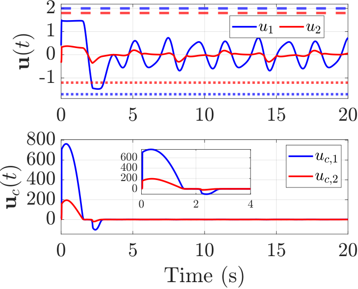

The corresponding results are presented in Figure 4. As shown in Figure 4(a), the system’s output converges to the reference trajectory after a brief transient of approximately . During the initial transient phase, the system requires high control effort to nullify the tracking errors, resulting in a higher commanded input , as evident from Figure 4(b). However, once the error is nullified, the control input demand decreases significantly. Note that despite this aggressive initial demand, the realized control inputs and strictly respect their individual asymmetric bounds at all times, as indicated by the dotted lines. The input phase portrait in Figure 4(c) confirms that the control trajectory remains entirely confined within the joint admissible set . The joint constraint evaluation , shown in Figure 4(d), closely approaches the critical boundary during peak demand but remains strictly non-positive throughout, as further verified by the plot, confirming that no joint constraint violation occurs.
We further demonstrate the proposed framework on the three-dimensional path-following guidance problem considered in [26]. The path-following problem is formulated as the pursuit of a virtual target moving along the desired path, with the relative range, elevation lead angle, and azimuth lead angle regulated to zero through the vehicle’s linear speed and pitch and yaw angular rates. In [26], the guidance inputs are constrained independently using isotropic realization, with each input restricted to its prescribed interval. However, such channel-wise constraints do not capture the common maneuvering authority shared by the pitch and yaw rate channels. To account for this coupling, we impose a joint constraint on the angular-rate commands and implement the resulting guidance inputs using AJ-APIR. The accompanying video https://youtu.be/21RK1Gd4fkY demonstrates the closed-loop response, where the vehicle converges to and follows the desired path while the realized angular rates satisfy both their individual bounds and the joint capacity constraint throughout the maneuver.
V Conclusions
This work developed an anisotropic admissibility-preserving control framework for multi-input strict-feedback nonlinear systems subject to a joint capacity constraint. The AJ-APIR uses the geometry of the joint constraint boundary to separate normal and tangential control directions. The normal component is attenuated as the boundary is approached, while the tangential component remains active, which prevents violation of joint constraints without unnecessarily restricting admissible control redistribution. The proposed AJ-APIR was then integrated with a recursive backstepping design, which demonstrates forward invariance of the joint admissible set and derives an explicit compact invariant set on which the realization channel remains uniformly nondegenerate. Under the proposed AJ-APC compatibility condition, the closed-loop system achieves exponential convergence of the tracking errors, while all closed-loop signals and the commanded input remain uniformly bounded. The numerical simulations show that satisfying individual actuator bounds does not ensure joint admissibility, whereas AJ-APIR preserves the shared capacity constraint during tracking.
References
- [1] (1999) Anti-windup for exponentially unstable linear systems. International Journal of Robust and Nonlinear Control: IFAC-Affiliated Journal 9 (10), pp. 701–716. Cited by: §I.
- [2] (2002) A common framework for anti-windup, bumpless transfer and reliable designs. Automatica 38 (10), pp. 1735–1744. Cited by: §I.
- [3] (2003) Antiwindup for stable linear systems with input saturation: an lmi-based synthesis. IEEE Transactions on Automatic Control 48 (9), pp. 1509–1525. Cited by: §I.
- [4] (1995) Nonlinear and adaptive control design. Wiley, New York. Cited by: §I.
- [5] (2011) Robust adaptive control of uncertain nonlinear systems in the presence of input saturation and external disturbance. IEEE Transactions on Automatic Control 56 (7), pp. 1672–1678. Cited by: 1st item, §I, §I.
- [6] (2011) Adaptive tracking control of uncertain MIMO nonlinear systems with input constraints. Automatica 47 (3), pp. 452–465. Cited by: 1st item, §I, §I.
- [7] (2009) Barrier lyapunov functions for the control of output-constrained nonlinear systems. Automatica 45 (4), pp. 918–927. Cited by: §I, §I.
- [8] (2005) Integrator backstepping using barrier functions for systems with multiple state constraints. In Proceedings of the 44th IEEE Conference on Decision and Control, pp. 8306–8312. Cited by: §I, §I.
- [9] (2016) Barrier lyapunov functions-based adaptive control for a class of nonlinear pure-feedback systems with full state constraints. Automatica 64, pp. 70–75. Cited by: §I, §I.
- [10] (2016) Control barrier function based quadratic programs for safety critical systems. IEEE Transactions on Automatic Control 62 (8), pp. 3861–3876. Cited by: §I, §I, §I.
- [11] (2019) Control barrier functions: theory and applications. In 2019 18th European Control Conference (ECC), pp. 3420–3431. Cited by: §I, §I, §I.
- [12] (2016) Constrained robot control using control barrier functions. In 2016 IEEE/RSJ International Conference on Intelligent Robots and Systems (IROS), pp. 279–285. Cited by: §I.
- [13] (1993) Constrained control allocation. Journal of Guidance, Control, and Dynamics 16 (4), pp. 717–725. Cited by: §I.
- [14] (2002) Evaluation of optimization methods for control allocation. Journal of Guidance, Control, and Dynamics 25 (4), pp. 703–711. Cited by: §I.
- [15] (2006) Constrained quadratic programming techniques for control allocation. IEEE Transactions on Control Systems Technology 14 (1), pp. 91–98. Cited by: §I.
- [16] (2013) Control allocation—a survey. Automatica 49 (5), pp. 1087–1103. Cited by: §I, §I, §I, §III.
- [17] (2005) Resolving actuator redundancy—optimal control vs. control allocation. Automatica 41 (1), pp. 137–144. Cited by: §I.
- [18] (2009) Dynamic allocation for input redundant control systems. Automatica 45 (6), pp. 1431–1438. Cited by: §I.
- [19] (2017) Reference and command governors for systems with constraints: a survey on theory and applications. Automatica 75, pp. 306–328. Cited by: §I.
- [20] (2020) Model predictive control: theory, computation, and design. Nob Hill Publishing. Cited by: §I.
- [21] (2026) Admissibility-preserving control for strict-feedback nonlinear systems with asymmetric actuator constraints. arXiv preprint arXiv:2608.15375. Cited by: 2nd item, §I, §I, §I, §II, §II, §III, §III, Remark 2.
- [22] (2026) Networked admissibility-preserving control for directed safe coordination. arXiv preprint arXiv:2609.09384. Cited by: §I.
- [23] (2004) Convex sets. In Convex Optimization, pp. 50–51. Cited by: §II.
- [24] (2024) Robust path-following guidance for an autonomous vehicle in the presence of wind. Aerospace Science and Technology 150, pp. 109225. Cited by: Remark 3.
- [25] (2024) Three-dimensional path-following nonlinear guidance for unmanned aerial vehicles. Journal of Guidance, Control, and Dynamics 47 (6), pp. 1231–1240. Cited by: Remark 3.
- [26] (2026) Three-dimensional nonlinear path-following guidance with bounded input constraints. Journal of Guidance, Control, and Dynamics 49 (1), pp. 198–215. External Links: Document Cited by: §IV.