PACT: End-to-End Learning of
Human Pose, Contacts, and Forces from Video

Rikhat Akizhanov¹ Yangsong Zhang¹ Nikolai Kaliazin¹ Peter Wolf² Yoshihiko Nakamura¹ Pascal Fua³ Fabio Pizzati¹ Ivan Laptev¹ ¹MBZUAI ²ETH Zürich ³EPFL {rikhat.akizhanov,ivan.laptev}@mbzuai.ac.ae Project page: https://rihat99.github.io/PACT/

Abstract

Human motion, environmental contacts, and interaction forces are governed by common physical laws, yet existing approaches typically separate visual pose reconstruction from contact and force estimation. This separation limits joint reasoning and can propagate errors between stages. We introduce PACT, an end-to-end model that jointly learns to estimate human pose, contacts and contact forces from monocular video. Our approach augments a human reconstruction foundation model with learnable contact-force tokens and a temporal transformer that integrates visual features with world-space motion. Joint prediction heads refine human poses and estimate contacts and forces, while physics-based supervision encourages consistency between the reconstructed motion and interaction forces. To address the scarcity of force annotations, we develop a data annotation pipeline that combines contact labeling with physics-based motion and force optimization, producing training supervision from synthetic and real-world videos. We also introduce a real-world climbing benchmark ForceWall with climbing videos and corresponding ground-truth contact forces obtained from the force sensors. Experiments demonstrate state-of-the-art contact and force estimation, outperforming staged reconstruction approaches and generalizing to interactions beyond the training distribution. These results support end-to-end joint learning as an effective approach to recovering human motion and physical interactions from video.

Refer to caption — Figure 1: End-to-end joint estimation of human pose, contacts, and forces with PACT. Predictions from monocular videos show generalization across diverse activities and support configurations. White meshes show estimated poses; yellow arrows show predicted forces at estimated contacts.

1 Introduction

Recovering human movement from video requires understanding both how the body moves and how it interacts with its environment. Recent advances in monocular human reconstruction have enabled increasingly accurate estimates of body shape and pose across diverse visual conditions. However, pose alone provides an incomplete description when interactions are involved: similar body configurations can correspond to different contact states and substantially different forces. Recovering these quantities is essential for analyzing physical effort, assessing athletic performance, and learning robot behaviors from human demonstrations. This motivates reconstructing human pose, environmental contacts, and interaction forces together from monocular videos.

Human motion, contacts and interaction forces are governed by common physical laws. Motion determines the required net forces and moments, while contacts determine where external forces can act. Conversely, contact and force constraints inform plausible body trajectories. Yet existing methods typically separate visual reconstruction from interaction estimation. Optimization-based approaches recover motion and forces using independently detected contacts and initial poses (Li et al., 2019). Learned dynamics models, including D&D (Li et al., 2022a) and PhysPT (Zhang et al., 2024), operate on reconstructed motion to infer physical quantities and refine trajectories. Their dynamics modules therefore receive a restricted representation of the video: intermediate errors can propagate, while visual evidence relevant to contacts and forces may be lost.

We investigate an end-to-end formulation that jointly learns pose, contact, and force estimation, retaining visual evidence while coupling motion and forces through physics. This is particularly relevant to sports, such as climbing, where support and load shift between hands and feet. Motion alone may not uniquely determine this force distribution, whereas video provides additional evidence about body configuration and surrounding supports. Combining visual observations with world-space motion enables the model to exploit these complementary cues.

Two challenges arise. First, the model must integrate visual and temporal information: contacts depend on the body’s relationship with its surroundings, while forces depend on motion over time. Human and camera motion must also be distinguished to reason about dynamics in a consistent frame. Second, force supervision is scarce. Force measurements require specialized hardware, and datasets with synchronized video, motion, contacts, and forces cover limited activities and environments.

In this work we introduce PACT, an end-to-end model for jointly estimating human Pose, contact states, And ConTact forces from monocular video. PACT builds on SAM 3D Body (Yang et al., 2026), retaining its pretrained visual backbone while learning modules for physical interaction estimation. Learnable contact-force tokens extract interaction-relevant visual features, and a temporal transformer combines these features with pose representations and world-space kinematics. Joint prediction heads refine the body trajectory and estimate contact probabilities and forces. A physics-based training objective couples the refined motion and predicted forces through the equations of motion, while contact predictions determine where the estimated forces are applied. This formulation preserves access to visual evidence while learning the three outputs within a shared model.

To train PACT, we develop an annotation pipeline that combines contact labeling with physics-based optimization of motion and forces. The pipeline produces supervision from synthetic sequences and real-world videos, expanding training coverage beyond datasets with directly measured forces. For evaluation, we introduce ForceWall, an instrumented climbing benchmark with measured contact forces and changing hand and foot supports. Experiments on ForceWall and established benchmarks demonstrate excellent results outperforming staged approaches. Notably our method demonstrates generalization to scenarios outside the training distribution. Figure 1 shows qualitative results of PACT across diverse scenes and motions. In summary, we propose the following contributions:

1. End-to-end joint estimation. We introduce PACT, a model that jointly learns human pose, contact, and force estimation from monocular video by combining pretrained visual representations, temporal reasoning, and physics-based supervision.

2. Training supervision and measured evaluation. We develop a physics-based annotation pipeline for synthetic and real-world videos and introduce ForceWall, a benchmark with directly measured contact forces for evaluating interactions with changing hand and foot supports.

3. Comprehensive empirical validation. We demonstrate state-of-the-art contact and force estimation across multiple benchmarks, generalization beyond the training distribution, and ablations that validate PACT’s architectural design choices and physical supervision.

2 Related Work

Human mesh recovery and world-grounded motion. The strongest regressors of parametric bodies (Loper et al., 2015; Pavlakos et al., 2019; Ferguson et al., 2025) in the camera frame (Goel et al., 2023; Patel and Black, 2025; Wang et al., 2025b; Yang et al., 2026) owe their accuracy to in-the-wild images whose labels were produced largely by fitting and by the models themselves (Kolotouros et al., 2019; Joo et al., 2021; Moon et al., 2022; Patel and Black, 2025), a scale that manual annotation cannot reach. World-frame motion needs the camera as well, from SLAM (Ye et al., 2023), learned motion priors (Shin et al., 2024; Wang et al., 2024) or gravity-view coordinates (Shen et al., 2024). These priors are learned from motion capture, mostly AMASS (Mahmood et al., 2019), whose people walk, run and sit on flat ground, and most of them rely on a floor for the scale of the camera or the contacts of the feet. We take this self-labeling route to the world frame, to contacts and to forces, with a world frame from a geometry model (Wang et al., 2025a; Wang et al., 2026) anchored to the size of the body rather than to a floor.

Contact estimation. Human-scene contact is estimated either as a dense label on the body surface, from images with BSTRO (Huang et al., 2022), DECO (Tripathi et al., 2023a) and InteractVLM (Dwivedi et al., 2025) or as a scene-constrained pose prior (Hassan et al., 2019), or as a sparse per-joint signal, typically foot contact, inside motion recovery (Rempe et al., 2020; Shin et al., 2024; Shen et al., 2024; Wang et al., 2025b). The first family learns from manual or scan-derived contact annotations and the second from motion capture, both scarce and the latter dominated by feet on a floor. Differently, we generate the labels from geometry and physics, with a scalable video-oriented pipeline, which we use to learn contact estimation end-to-end.

Physics-based force estimation. Brubaker et al. (2009) inferred contact forces and joint torques from motion, and Li et al. (2019); Li et al. (2022c) recover motion and contact forces by trajectory optimization given a ground plane and contacts in 2D, and Gärtner et al. (2022) through a physics simulator. Physics has since served to refine poses (Rempe et al., 2020; Shimada et al., 2020; Xie et al., 2021; Tripathi et al., 2023b), as weak supervision for learned forces (Zell et al., 2020; Ehsani et al., 2020), and as a regression target: D&D (Li et al., 2022a), PhysPT (Zhang et al., 2024), MusclePose (Zhu et al., 2025) and ImDy (Liu et al., 2025) predict forces, torques or muscle activations from a reconstructed motion, trained on motion capture or simulation. Biomechanics pipelines estimate ground reaction forces with a musculoskeletal model, by simulation from multi-view (Uhlrich et al., 2023) or, with learned kinematics, monocular video (Gilon et al., 2026). GaitDynamics (Tan et al., 2026) assumes motion-capture poses and the ground-truth mass. Most of these take a flat floor as the support and the feet as the contacts, Li et al. (2019) and Gärtner et al. (2022) also handle hand-held objects and scene geometry given the contacts, and all of them read the forces from a motion rather than from the image. We instead jointly predict contacts and forces from the image.

3 Method

We aim to estimate human motion, contacts, and contact forces from a monocular video. While individual frames provide evidence about body configuration and possible contacts, forces also depend on how the body moves over time. Hence, we use a temporal transformer to combine world-informed image features, extracted with a pretrained body reconstruction foundation model, over time. This preserves the generalization capabilities of the foundation model, learning new time-dependent outputs too (Section 3.1). Since physics-related data annotation required for training is challenging, we use a physics-based data annotation pipeline, compatible with in-the-wild videos, in Section 3.2.

3.1 Architecture

3.1.1 Feature extraction

Preliminaries.

Our architecture is in Figure 2. We build on SAM 3D Body (Yang et al., 2026), which produces pose tokens that can be decoded into body and camera parameters from arbitrary frames. These features provide an informative representation of human geometry, allowing us to learn generalizable contact and force estimation without learning body reconstruction from scratch.

Let $\mathbf{x}=(\mathbf{x}_{t})_{t=1}^{T}$ denote an input video. We obtain masks $\mathbf{s}_{t}$ of the tracked person using SAM 3 (Carion et al., 2026) and process each frame independently, $\mathbf{p}_{t}=\operatorname{SAM3D}(\mathbf{x}_{t},\mathbf{s}_{t})$ . Here, $\mathbf{p}_{t}$ contains the pose tokens for frame $t$ . We use body and camera heads, $\mathcal{H}_{\mathrm{SMPL\text{-}X}}$ and $\mathcal{H}_{\mathrm{camera}}$ , to decode these tokens into parameters that jointly determine the camera-frame body configuration $\mathbf{q}_{t}^{c}$ . While SAM 3D Body provides pretrained heads, we retrain these heads for compatibility with SMPL-X to reduce engineering complexity, while keeping the pretrained backbone frozen. $\mathbf{q}_{t}^{c}$ contains root translation, root and joint rotations, and shape, obtained from the two heads as follows:

\displaystyle(\bm{\theta}_{t}^{c},\bm{\beta}_{t})=\mathcal{H}_{\mathrm{SMPL\text{-}X}}(\mathbf{p}_{t}),\quad\bm{\kappa}_{t}=\mathcal{H}_{\mathrm{camera}}(\mathbf{p}_{t}),\quad\mathbf{q}_{t}^{c}=\left(\mathbf{r}_{t}^{c},\bm{\theta}_{t}^{c},\bm{\beta}\right).

(1)

Here, $\bm{\kappa}_{t}$ contains the camera parameters used to recover the camera-frame root translation $\mathbf{r}_{t}^{c}$ from the crop box and focal length. The parameters $\bm{\theta}_{t}^{c}$ contain the root orientation in camera coordinates and the local joint rotations. We fix shape $\bm{\beta}$ across the video by averaging the framewise predictions $\bm{\beta}_{t}$ , since changes in shape should not explain changes in motion.

Contact-force tokens.

Contacts and forces depend on the human configuration, so a foundational 3D human reconstruction model should provide generalizable features for the task. Hence, we follow the principle of Visual Prompt Tuning (Jia et al., 2022) to introduce a learnable input embedding and corresponding output tokens on top of SAM 3D Body, retaining the backbone weights frozen. Doing so, we benefit from generalization capabilities of the backbone. The output becomes:

(\mathbf{p}_{t},\mathbf{z}_{t}^{\prime})=\operatorname{SAM3D}(\mathbf{x}_{t},\mathbf{s}_{t};\mathbf{z}_{t}).

(2)

Above, $\mathbf{z}_{t}$ contains learned input embeddings, while $\mathbf{z}_{t}^{\prime}$ contains their image-dependent outputs. Each token corresponds to one contact point: we use 35 contacts at different surface points of the human body. The points are listed in Appendix A.2 and shown in Figure 5.

World-informed poses.

The pose tokens $\mathbf{p}_{t}$ and corresponding body predictions $\mathbf{q}_{t}^{c}$ are camera-relative. As such, they mix human and camera motion, having different implications for force estimation. We therefore combine these visual features with explicit world-space kinematics to describe body motion independently of the camera. Using camera poses from VGGT- $\Omega$ (Wang et al., 2026) and video-level scale alignment with the metric body estimate, we transform $\mathbf{q}_{t}^{c}$ into world-space configurations $\mathbf{q}_{t}$ . From the resulting trajectory $\mathbf{q}=(\mathbf{q}_{t})_{t=1}^{T}$ , we extract SMPL-X joint positions $\mathbf{j}_{t}$ relative to the root and their velocities $\dot{\mathbf{j}}_{t}$ , in the body frame, computed from previous and following frames using elapsed time. Two MLPs map the pose tokens and these kinematics before concatenation:

\mathbf{p}_{t}^{\prime}=\left(\operatorname{MLP}_{\mathrm{pose}}(\mathbf{p}_{t}),\operatorname{MLP}_{\mathrm{world}}(\mathbf{j}_{t},\dot{\mathbf{j}}_{t})\right).

(3)

Parentheses denote concatenation. The resulting $\mathbf{p}_{t}^{\prime}$ provides pose context while adding world-space motion information for contact and force estimation.

3.1.2 Predicting motion, contacts, and forces

Temporal aggregation.

Similar body configurations can imply different contact forces, making an instantaneous pose insufficient for force estimation. We therefore aggregate the pose and contact-force features over time, allowing the model to relate changes in body motion to the evolution of contacts. We introduce a temporal transformer $\mathcal{T}$ with three standard blocks. The full architecture is described in Appendix B.4. We then have:

(\mathbf{p}_{t}^{\prime\prime},\mathbf{z}_{t}^{\prime\prime})_{t=1}^{T}=\mathcal{T}\left((\mathbf{p}_{t}^{\prime},\mathbf{z}_{t}^{\prime})_{t=1}^{T}\right).

(4)

Temporal attention connects observations of the same body region, while attention across slots allows its prediction to depend on the whole-body configuration and the other contacts. We use RoPE embeddings (Su et al., 2024) in temporal attention to account for the relative temporal position of observations. The time-informed outputs remain associated with individual frames: $\mathbf{p}_{t}^{\prime\prime}$ describes the body at time $t$ , and $\mathbf{z}_{t}^{\prime\prime}$ contains its contact-force tokens.

Prediction heads.

We finally map the tokens to outputs. First, we introduce two separate prediction heads $\mathcal{H}_{\text{contacts}}$ for contacts $\hat{\mathbf{c}}$ and $\mathcal{H}_{\text{force}}$ for forces $\tilde{\mathbf{f}}$ , both processing the $\mathbf{z}_{t}^{\prime\prime}$ tokens.

\displaystyle\hat{\mathbf{c}}_{t}=\sigma\!\left(\mathcal{H}_{\mathrm{contacts}}(\mathbf{z}_{t}^{\prime\prime})\right),\quad\tilde{\mathbf{f}}_{t,k}=\mathcal{H}_{\mathrm{force}}(\mathbf{z}_{t,k}^{\prime\prime}),\quad\hat{\mathbf{f}}_{t,k}=\hat{c}_{t,k}\,mg\,\mathbf{R}_{t}\,\tilde{\mathbf{f}}_{t,k}.

(5)

Here, $\sigma$ is a sigmoid for extracting contact probabilities. Considering that forces can exist only in presence of a contact, we use the contact probabilities $\hat{c}_{t,k}$ to gate the forces for each contact point. The head regresses $\tilde{\mathbf{f}}_{t,k}$ in the body frame in body weights, and the root orientation $\mathbf{R}_{t}$ and mass $m$ convert it to world newtons (Appendix B.5). Gravity is a unit direction in world coordinates, with $g=9.81$ m/s² fixed.

We also use a pose refinement head $\mathcal{H}_{\mathrm{offset}}$ used to correct SAM 3D Body pose output. Framewise prediction can indeed introduce inconsistencies affecting force estimation, which we correct with temporal information. We predict offsets in the body frame with a head $\mathcal{H}_{\mathrm{offset}}$ . A gravity head $\mathcal{H}_{\text{gravity}}$ processes $\mathbf{p}_{t}^{\prime\prime}$ to extract the gravity direction $\hat{\mathbf{g}}$ , taking into account tilted cameras:

\hat{\mathbf{q}}_{t}=\mathbf{q}_{t}\oplus\mathcal{H}_{\mathrm{offset}}(\mathbf{p}_{t}^{\prime\prime}),\quad\hat{\mathbf{g}}_{t}=\mathcal{H}_{\text{gravity}}(\mathbf{p}_{t}^{\prime\prime}).

(6)

The per-frame estimates $\hat{\mathbf{g}}_{t}$ are averaged over the clip into $\hat{\mathbf{g}}$ (Appendix B.5). The operator $\oplus$ adds a root translation offset and composes rotation corrections with the root and body-joint rotations, leaving the shape unchanged. Predicting corrections allows the model to retain the initial reconstruction while adjusting it using neighboring observations.

Iterative refinement.

Inspired by iterative refinement in SAM 3D Body (Yang et al., 2026), we apply the shared offset head after each transformer block, starting from $\hat{\mathbf{q}}_{t}^{(0)}=\mathbf{q}_{t}$ . At block $i$ , we compute $\hat{\mathbf{q}}_{t}^{(i)}=\hat{\mathbf{q}}_{t}^{(i-1)}\oplus\mathcal{H}_{\mathrm{offset}}(\mathbf{p}_{t}^{\prime\prime(i)})$ , where $\mathbf{p}_{t}^{\prime\prime(i)}$ denotes the block’s pose features. From the refined trajectory, we recompute joint positions $\mathbf{j}_{t}^{(i)}$ and velocities $\dot{\mathbf{j}}_{t}^{(i)}$ , and add them, with the current contact and gravity estimates, to the pose features (Equation 23). These features inform the next block with intermediate estimates of refined body motion. After the three blocks, $\hat{\mathbf{q}}_{t}=\hat{\mathbf{q}}_{t}^{(3)}$ and the offset of Equation 6 is their composition.

3.2 Data and training

3.2.1 Data construction

Physics modeling.

No dataset of in-the-wild videos carries poses, contacts and forces together, so we design a force and contacts optimization pipeline used to annotate existing videos. We consider the body as the floating-base articulated rigid body of SMPL-X in the configuration $\mathbf{q}_{t}$ of Section 3.1, with segment masses and inertias derived from the shaped mesh as in PhysPT (Zhang et al., 2024), and $K=35$ contact points on its surface, each with an outward normal (Appendix A.2). For a trajectory $\mathbf{q}$ and related velocity and acceleration $\dot{\mathbf{q}},\ddot{\mathbf{q}}$ , the contact forces $\mathbf{f}_{t}=(\mathbf{f}_{t,k})_{k=1}^{K}$ respect the recursive Newton–Euler algorithm (RNEA) (Featherstone, 2008):

\bm{\tau}_{t}=\mathbf{M}(\mathbf{q}_{t})\,\ddot{\mathbf{q}}_{t}+\mathbf{b}(\mathbf{q}_{t},\dot{\mathbf{q}}_{t})+\mathbf{G}(\mathbf{q}_{t})-\mathbf{J}(\mathbf{q}_{t})^{\top}\mathbf{f}_{t},

(7)

with $\mathbf{M}$ , $\mathbf{b}$ and $\mathbf{G}$ the inertia, Coriolis and gravity terms and $\mathbf{J}$ the Jacobian of the contact points. The variable $\bm{\tau}_{t}$ is composed of the force $\bm{\tau}^{f}_{t}$ , the moment $\bm{\tau}^{m}_{t}$ at the unactuated root (vanishing when the forces explain the motion), and the joint torques $\tau_{t,j}$ .

Pseudo labeling.

We obtain pseudo labels for contacts and forces by assuming knowledge of the 3D scene. This is trivial in simulation. For in-the-wild videos, we track the person with SAM 3 (Carion et al., 2026), reconstruct the scene cloud with normals with VGGT- $\Omega$ (Wang et al., 2026), and extract 2D keypoints with Sapiens2 (Khirodkar et al., 2026) and SAM 3D Body per frame. Sapiens2, specialized on keypoints, adds 2D reprojection supervision to the initial SAM 3D Body pose. With the 3D scene, we label a point in contact, $c^{*}_{t,k}=1$ , when it is near the scene and still, or when the root wrench of the motion cannot be explained without it. The full pipeline is in Appendix A.

For labeling forces, we use a kinematic objective $E_{\text{kin}}(\mathbf{q})$ derived from Li et al. (2019), with additional constraints for trajectory smoothing, depth and penetration, detailed in Appendix A.3. We use it to solve for the forces and the motion together:

\mathbf{q}^{*},\mathbf{f}^{*}=\arg\min_{\mathbf{q},\,\mathbf{f}}\;E_{\text{kin}}(\mathbf{q})+\sum_{t}\Big(w_{F}\,\frac{\|\bm{\tau}^{f}_{t}\|^{2}}{(mg)^{2}}+w_{T}\,\frac{\|\bm{\tau}^{m}_{t}\|^{2}}{(mg\ell)^{2}}+w_{J}\sum_{j}\mu_{j}\,\frac{\tau_{t,j}^{2}}{(mg\ell)^{2}}\Big)+E_{\text{reg}}(\mathbf{q},\mathbf{f}),

(8)

with $m$ the body mass derived from shape (Zhang et al., 2024), $\ell=1$ m a unit lever that only makes the moment terms dimensionless like the force terms, $w_{F}$ , $w_{T}$ , $w_{J}$ the term weights, $\mu_{j}$ per-joint multipliers (Appendix A.4) and $E_{\text{reg}}$ a regularizer on the magnitude and smoothness of forces and torques. Each $\mathbf{f}_{t,k}$ is restricted to the labeled contacts and to a friction cone about the normal of its point (Appendix A.4). By optimizing $\mathbf{q}^{*}$ as well, we simultaneously improve forces and obtain signal for a smoothed pose prediction. Contacts are re-read on the smoothed trajectory before the force solve (Appendix A.2). Every label carries a confidence, for contacts from the stillness of the point and for forces from how well they close the equations of motion (Appendix A.5).

3.2.2 Losses

Pose, contacts, and forces.

The per-frame SMPL-X ( $\mathcal{H}_{\text{SMPL-X}}$ ) and camera ( $\mathcal{H}_{\text{camera}}$ ) heads are trained as in HMR 2.0 (Goel et al., 2023) with the full-frame projection of CLIFF (Li et al., 2022b). The gravity head $\mathcal{H}_{\text{gravity}}$ is supervised with the gravity of the labels, which GeoCalib (Veicht et al., 2024) estimates from the video (Appendix A.6). The corrected trajectory $\hat{\mathbf{q}}_{t}$ of Equation 6 is supervised on its joints, rotations and world root, and on the velocities of its joints and root orientation, so that the model matches how the labels move rather than only where they are (Appendix B.6). With $c^{*}_{t,k}\in\{0,1\}$ and $\mathbf{f}^{*}_{t,k}$ the contact and force labels of point $k$ from Equation 8, the latter rotated to the body frame and divided by $mg$ , $\bar{c}^{*}_{t,k}$ the contacts re-read for the force solve, $w^{\text{c}}_{t,k}$ and $w^{\text{f}}_{t}$ their confidences, $\hat{c}_{t,k}$ the contact probability of Equation 5 and $\tilde{\mathbf{f}}_{t,k}=\mathcal{H}_{\mathrm{force}}(\mathbf{z}^{\prime\prime}_{t,k})$ the force before gating, the losses are:

\mathcal{L}_{\text{c}}=\sum_{t,k}w^{\text{c}}_{t,k}\,\operatorname{BCE}(\hat{c}_{t,k},c^{*}_{t,k}),\qquad\mathcal{L}_{\text{f}}=\sum_{t,k}w^{\text{f}}_{t}\Big[\bar{c}^{*}_{t,k}\,\rho(\tilde{\mathbf{f}}_{t,k}-\mathbf{f}^{*}_{t,k})+(1-\bar{c}^{*}_{t,k})\,\|\tilde{\mathbf{f}}_{t,k}\|\Big],

(9)

a Huber loss $\rho$ on the points in contact and a penalty on force predicted at a free point, complemented by terms on the force magnitude and on the net force (Appendix B.6).

Physics.

Since PACT predicts forces, contacts and poses, we can also use Equation 7 as a loss for physical consistency, applied to the gated world forces $\hat{\mathbf{f}}_{t,k}$ of Equation 5:

\mathcal{L}_{\text{phys}}=\sum_{t}\Big(\lambda_{F}\,\rho_{\delta_{F}}\Big(\frac{\bm{\tau}^{f}_{t}}{mg}\Big)+\lambda_{T}\,\rho_{\delta_{T}}\Big(\frac{\bm{\tau}^{m}_{t}}{mg\ell}\Big)+\lambda_{J}\sum_{j}\mu_{j}\,\frac{\tau_{t,j}^{2}}{(mg\ell)^{2}}\Big).

(10)

The full derivation is in Appendix B.7. In the equation, $\rho_{\delta}$ is a pseudo-Huber loss of scale $\delta$ per component, with the weights $\lambda$ and scales $\delta$ listed in Appendix B.6. A stillness term $\mathcal{L}_{\text{still}}$ penalizes the world speed of a contact point on the frames where it is labeled in contact, so that the corrected body does not slide on its supports (Equation 27 in Appendix B.6). We backpropagate the loss alongside all the supervised losses in an end-to-end fashion.

4 Experiments

4.1 Datasets and metrics

Training data.

We train on BEDLAM2 (Tesch et al., 2025), 18,076 sequences and 5.5M frames of 26,178 people labeled as in Section 3.2.1 (Appendix A.7), and on ClimbingVideos, a new dataset of YouTube indoor climbing and bouldering videos labeled with the same pipeline. We curate it by keyword search, vision-language models on the thumbnail and the video (Deitke et al., 2025; Clark et al., 2026), shot detection, a full-body pose gate (Jocher et al., 2026) and one manual review (Appendix C.1). It holds 1,528 scenes from 191 videos, 4.5 hours at 24 to 60 fps, split by source video into 1,419 training scenes (460k frames) and 109 test scenes (31k frames) with manual contact labels for 14 joints. We train on both.

Evaluation benchmarks.

We evaluate forces and contacts against measured ground truth. For forces, the parkour sequences of Li et al. (2019) (Parkour) are 28 clips of vaults, muscle-ups and pull-ups with motion capture and forces from plates at the feet and a bar at the hands. The OpenCap benchmark (Uhlrich et al., 2023) has smartphone videos of walking, squatting, standing up from a chair and dropping from a box over force plates (OC-All), of which 22 walking trials form OC-Walking for comparison with published results (Gilon et al., 2026) (Appendix C.5). Our new ForceWall test set is a bouldering wall whose four panels, one under each limb, rest on three-axis force sensors: two climbers boulder at $0^{\circ}$ , $16^{\circ}$ and $32^{\circ}$ overhang, 68 clips and 29.6k scored frames from one of three calibrated cameras (Figure 8, Appendix C.2). Sensors are matched to limbs with the reconstructed body, and a limb is in contact when its sensor reads 50 N, until it drops below 30 N. We evaluate contacts on the ClimbingVideos test set, ForceWall and RICH (Huang et al., 2022).

Metrics.

Contacts are scored by precision, recall and F1 at threshold 0.5, micro-averaged over frames and limbs. The force of a limb is the sum of its contact points, and its error is the mean norm of the difference to the sensor over all frames in newtons (MAE). We add the mean angle between estimated and measured force where both exceed 50 N (Angle), the Pearson correlation of the magnitudes over frames and limbs (Corr), the load-share error (Share), the mean absolute difference between a limb’s share of the load and the measured one, in percentage points (pp), and the physical root residual, the mean root force and moment of Equation 7 left by a method’s own motion and forces, in body weights (bw), which measures how consistent poses and forces are. Poses are evaluated with MPJPE, on ForceWall against a multi-view fit and on Parkour with the similarity-aligned MPJPE of its evaluator (Appendix C.4). On OpenCap we follow the benchmark protocol and report the mean absolute error of each foot’s ground reaction force per axis in percent of body weight (Appendix C.5).

4.2 Contacts

We compare with BSTRO (Huang et al., 2022), trained on RICH, DECO (Tripathi et al., 2023a), trained on RICH and other data, and InteractVLM (Dwivedi et al., 2025), trained on the same data, a promptable contact detector prompted with “scene”, as its authors recommend, and with “wall” for climbing. We add human reconstruction methods with contact heads, GVHMR (Shen et al., 2024) and PromptHMR (Wang et al., 2025b). In Table 1 we are best on ClimbingVideos and ForceWall and first on RICH in precision (0.941) and second in F1 (0.856). Since BSTRO (best) is trained on RICH, we achieve almost the same performance on a domain fully out-of-distribution, which proves the generalization of PACT.

Table 1: Contacts benchmarks. We compare on ClimbingVideos, the sensor contacts of ForceWall, and the contact annotations of RICH. We are best on climbing datasets and highly competitive on RICH against methods that have seen its training set. For PACT, RICH is completely out-of-distribution. Best is bold, second is underlined.

	ClimbingVideos			ForceWall			RICH
Method	Prec. $\uparrow$	Rec. $\uparrow$	F1 $\uparrow$	Prec. $\uparrow$	Rec. $\uparrow$	F1 $\uparrow$	Prec. $\uparrow$	Rec. $\uparrow$	F1 $\uparrow$
BSTRO (Huang et al., 2022)	0.472	0.518	0.494	0.840	0.454	0.590	0.800	0.937	0.863
DECO (Tripathi et al., 2023a)	0.435	0.594	0.502	0.821	0.548	0.658	0.736	0.751	0.744
InteractVLM (Dwivedi et al., 2025), “scene”	0.419	0.503	0.457	0.830	0.604	0.699	0.833	0.855	0.844
InteractVLM (Dwivedi et al., 2025), “wall”	0.738	0.849	0.789	0.820	0.676	0.741	0.785	0.669	0.722
GVHMR (Shen et al., 2024)	0.559	0.441	0.493	0.892	0.680	0.772	0.814	0.746	0.778
PromptHMR (Wang et al., 2025b)	0.504	0.517	0.510	0.852	0.706	0.772	0.790	0.814	0.802
PACT	0.948	0.895	0.921	0.896	0.980	0.936	0.941	0.784	0.856

4.3 Force estimation

Benchmark results.

Our closest baselines are Li et al. (2019) and PhysPT (Zhang et al., 2024). We report the published results of Li et al. (2019) and also feed their algorithm the SAM 3D Body poses that we start from, an improved “Li et al. (2019)++”. PhysPT also receives SAM 3D Body poses. A naive inverse dynamics baseline estimates contacts with InteractVLM (“wall”) and applies Equation 7 to extract forces, and we report the MPJPE of its smoothed SAM 3D Body poses. We significantly outperform all baselines on both ForceWall and Parkour, so our method extends to different types of motion and yields robust force estimation (Table 2). In particular, the gap in Pearson correlation with the measured forces (0.725 vs 0.243 for the second best on ForceWall) backs the physical validity of our output.

For other scenarios, we follow the OpenCap evaluation pipeline (Uhlrich et al., 2023) and report in Table 3 the foot force errors along the vertical (Vert), anteroposterior (AP) and mediolateral (ML) axes on OC-Walking and OC-All, against published OpenCap (Uhlrich et al., 2023) and OpenCap-mono (Gilon et al., 2026) results and the previous baselines, with the ground-truth mass and with the mass estimated from shape. We beat all baselines except two-view OpenCap in some scenarios (3.5 vs 3.7 in OC-All), where PACT is monocular. The estimated mass changes the results little, suggesting robustness.

In-the-wild evaluation.

Figure 3 shows YouTube videos of different sports. PACT yields realistic forces even without ground truth: higher forces for pushes (leftmost frames) before a jump (top) or a complex motion (bottom), and realistic contacts and forces in unusual poses holding hands (right). Our annotation pipeline (Optimization) fails completely on these videos, so by curating a dataset and training on it, PACT generalizes beyond the capabilities of its own annotation pipeline, thanks to the rich contact-force tokens benefiting from SAM 3D Body priors. More results in Appendix E.4. Please also refer to our project page for examples in motion.

Table 2: Force estimation benchmarks. We outperform other methods in force MAE and correlation, reach the lowest moment residual and improve the poses of SAM 3D Body on Parkour.

	Method	MPJPE [mm] $\downarrow$	Force MAE [N] $\downarrow$					Force agreement			Residual $\downarrow$
	Method	MPJPE [mm] $\downarrow$	L. foot	R. foot	L. hand	R. hand	Avg.	Angle [^∘] $\downarrow$	Corr $\uparrow$	Share [pp] $\downarrow$	Force [bw]	Moment [bw m]
ForceWall	SAM 3D Body	42.8	–	–	–	–	–	–	–	–	–	–
	Li et al. (2019)++	137.4	166.2	141.5	128.8	129.1	141.4	21.2	0.243	18.5	0.384	0.113
	PhysPT	86.7	193.8	147.4	170.3	159.8	167.8	21.4	0.169	28.0	0.785	0.080
	Inverse dynamics	42.7	200.7	162.2	166.0	192.4	180.3	28.8	0.007	21.9	0.024	0.040
	PACT	49.1	98.4	90.4	72.9	80.4	85.5	14.4	0.725	8.7	0.167	0.038
Parkour	SAM 3D Body	68.9	–	–	–	–	–	–	–	–	–	–
	Li et al. (2019)	122.1	144.2	138.2	107.9	113.4	125.9	–	–	–	–	–
	Li et al. (2019)++	95.3	132.2	134.8	98.7	74.6	110.1	17.1	0.551	10.8	0.431	0.066
	PhysPT	73.1	147.2	142.1	132.5	91.1	128.2	10.3	0.156	32.7	0.891	0.092
	Inverse dynamics	68.7	163.2	126.2	187.1	205.8	170.6	23.8	0.527	18.7	0.042	0.073
	PACT	66.3	117.1	148.4	77.9	66.3	102.4	16.7	0.712	14.6	0.283	0.044

Table 3: Evaluation on OpenCap data. We outperform all methods in all metrics except two-view OpenCap, where we are monocular. We report results with each method’s estimated mass and with the measured mass, and published numbers for OpenCap and OpenCap-mono.

Method	Input	Type	OC-Walking						OC-All
			Estimated mass			True mass			Estimated mass			True mass
			Vert.	AP	ML	Vert.	AP	ML	Vert.	AP	ML	Vert.	AP	ML
OpenCap (Uhlrich et al., 2023)	two views	simulation	–	–	–	12.2	3.1	1.2	–	–	–	11.4	3.5	3.8
OpenCap-mono (Gilon et al., 2026)	one view	learn + optim.	–	–	–	9.7	4.4	1.7	–	–	–	–	–	–
PhysPT (Zhang et al., 2024)	one view	learned	66.3	8.0	2.5	64.8	8.0	2.5	46.0	4.1	3.9	45.9	4.2	4.0
Li et al. (2019)++	one view	optimization	33.9	9.0	4.1	35.0	8.6	4.0	37.0	6.1	4.3	36.5	5.8	4.3
PACT	one view	learned	11.8	3.0	1.5	7.8	3.3	1.6	11.6	3.4	2.3	9.7	3.7	2.4

4.4 Ablations

Table 4 ablates first the architecture (top), trained on ClimbingVideos only for compute reasons and tested on ForceWall. Adding our contributions in sequence yields the best force accuracy. The temporal transformer alone prioritizes pose estimation, but our contributions substantially increase force accuracy (87.5 N) and Pearson correlation (0.729), and removing the contact head (No contact head) significantly degrades the forces, showing the benefit of multitask learning. On training data (bottom), combining BEDLAM2 with ClimbingVideos enlarges the training distribution and compensates for suboptimal pose optimization: MPJPE improves substantially with more data (56.6 vs 49.1) while the other metrics barely move. The temporal transformer is further ablated in Appendix E.2.

Table 4: Ablations on ForceWall. Architecture additions are cumulative (Appendix E.1), with the physics loss completing the full model. The training-data ablation uses the full model. The full model reaches the best force accuracy.

Architecture (ClimbingVideos training)
Setup	Pose	Contacts	Forces				Residual
Setup	MPJPE [mm] $\downarrow$	F1 $\uparrow$	MAE [N] $\downarrow$	Angle [^∘] $\downarrow$	Corr $\uparrow$	Share [pp] $\downarrow$	Force [bw] $\downarrow$	Moment [bw m] $\downarrow$
Per-frame tokens and heads	72.9	0.895	120.1	22.1	0.472	12.2	0.471	0.096
+ temporal transformer	50.5	0.914	102.2	17.3	0.649	10.2	0.422	0.075
+ world-informed poses	61.2	0.914	117.2	21.2	0.504	11.6	0.291	0.075
+ iterative refinement	57.7	0.917	112.0	19.9	0.578	11.0	0.286	0.073
+ contact-force tokens	55.4	0.936	96.0	18.1	0.711	8.9	0.240	0.076
+ physics loss (ours)	56.6	0.936	87.5	15.0	0.729	8.6	0.155	0.037
No contact head	60.2	–	122.7	14.9	0.562	10.8	0.130	0.026
Training data
ClimbingVideos	56.6	0.936	87.5	15.0	0.729	8.6	0.155	0.037
BEDLAM2	60.0	0.561	153.0	16.4	0.410	24.2	0.445	0.051
Both (ours)	49.1	0.936	85.5	14.4	0.725	8.7	0.167	0.038

5 Conclusions

We presented PACT, an end-to-end model jointly estimating human pose, contacts and forces from monocular video. Our architecture combines pretrained visual representations with world-space motion, temporal refinement, and physics-based supervision. We also introduced an annotation pipeline for synthetic and real-world videos, and ForceWall for evaluation against measured forces. Experiments show accurate contact and force estimation and generalization beyond the training distribution to RICH, Parkour, OpenCap and in-the-wild videos without retraining. They highlight the effectiveness of combining visual evidence and physical reasoning to recover human interactions across activities and environments.

Acknowledgements

This work was in part supported by the Institute of Information & communications Technology Planning & Evaluation (IITP) grant funded by the Korean government (MSIT) (No. RS-2024-00457882, National AI Research Lab Project).

Ethics statement

ClimbingVideos is built from publicly available YouTube videos of climbers. We release only derived annotations (tracks, body parameters, contacts, forces and confidences) together with video identifiers and time stamps, not the videos themselves, and we will honour removal requests. The automatic gates reject clips showing children. ForceWall was recorded with the informed consent of the participating climbers. The method estimates forces from video without contact with the subject, and we do not foresee harmful uses beyond those of general human motion capture.

Reproducibility statement

The curation rules and their thresholds are given in Section 4.1 and Appendix C, the labeling optimization with its objectives and weights in Section 3.2.1 and Appendix A, the model, losses and training schedule in Section 3.1, Section 3.2.2 and Appendix B, and every metric in Appendix C. Code for the pipeline, the model and the evaluation scripts, together with the dataset annotations, the test-split manual labels and the benchmark recordings, will be released.

References

Aharon et al. (2022) N. Aharon, R. Orfaig, and B. Bobrovsky BoT-SORT: robust associations multi-pedestrian tracking. External Links: 2206.14651, Link Cited by: §C.1.
Anderson et al. (2007) D. E. Anderson, M. L. Madigan, and M. A. Nussbaum Maximum voluntary joint torque as a function of joint angle and angular velocity: model development and application. Journal of Biomechanics 40 (14), pp. 3105–3113. Cited by: §A.4.
Brubaker et al. (2009) M. A. Brubaker, L. Sigal, and D. J. Fleet Estimating contact dynamics. In ICCV, Cited by: §2.
Carion et al. (2026) N. Carion, L. Gustafson, Y. Hu, S. Debnath, R. Hu, D. S. Coll-Vinent, C. Ryali, K. V. Alwala, H. Khedr, A. Huang, J. Lei, T. Ma, B. Guo, A. Kalla, M. Marks, J. Greer, M. Wang, P. Sun, R. Rädle, T. Afouras, E. Mavroudi, K. Xu, T. Wu, Y. Zhou, L. Momeni, R. Hazra, S. Ding, S. Vaze, F. Porcher, F. Li, S. Li, A. Kamath, H. K. Cheng, P. Dollar, N. Ravi, K. Saenko, P. Zhang, and C. Feichtenhofer SAM 3: segment anything with concepts. In ICLR, Cited by: §A.1, §3.1.1, §3.2.1.
Clark et al. (2026) C. Clark, J. Zhang, Z. Ma, J. S. Park, R. Tripathi, S. Lee, M. Salehi, J. Ren, C. D. Kim, Y. Yang, V. Shao, Y. Yang, W. Huang, Z. Gao, T. Anderson, J. Zhang, J. Jain, G. Stoica, A. Farhadi, and R. Krishna Molmo2: open weights and data for vision-language models with video understanding and grounding. In CVPR, Cited by: §C.1, §4.1.
Deitke et al. (2025) M. Deitke, C. Clark, S. Lee, R. Tripathi, Y. Yang, J. S. Park, M. Salehi, N. Muennighoff, K. Lo, L. Soldaini, J. Lu, T. Anderson, E. Bransom, K. Ehsani, H. Ngo, Y. Chen, A. Patel, M. Yatskar, C. Callison-Burch, A. Head, R. Hendrix, F. Bastani, E. VanderBilt, N. Lambert, Y. Chou, A. Chheda, J. Sparks, S. Skjonsberg, M. Schmitz, A. Sarnat, B. Bischoff, P. Walsh, C. Newell, P. Wolters, T. Gupta, K. Zeng, J. Borchardt, D. Groeneveld, C. Nam, S. Lebrecht, C. Wittlif, C. Schoenick, O. Michel, R. Krishna, L. Weihs, N. A. Smith, H. Hajishirzi, R. Girshick, A. Farhadi, and A. Kembhavi Molmo and PixMo: open weights and open data for state-of-the-art vision-language models. In CVPR, Cited by: §4.1.
Delp et al. (1996) S. L. Delp, A. E. Grierson, and T. S. Buchanan Maximum isometric moments generated by the wrist muscles in flexion-extension and radial-ulnar deviation. Journal of Biomechanics 29 (10), pp. 1371–1375. External Links: ISSN 0021-9290 Cited by: §A.4.
Dempster (1955) W. T. Dempster Space requirements of the seated operator. Technical report Vol. 55, Wright-Patterson Air Force Base Ohio. Cited by: §A.4.
Dwivedi et al. (2025) S. K. Dwivedi, D. Antić, S. Tripathi, O. Taheri, C. Schmid, M. J. Black, and D. Tzionas InteractVLM: 3D interaction reasoning from 2D foundational models. In CVPR, Cited by: §2, §4.2, Table 1, Table 1.
Ehsani et al. (2020) K. Ehsani, S. Tulsiani, S. Gupta, A. Farhadi, and A. Gupta Use the force, Luke! learning to predict physical forces by simulating effects. In CVPR, Cited by: §2.
Featherstone (2008) R. Featherstone Rigid body dynamics algorithms. Springer. External Links: ISBN 978-0-387-74314-1, Document Cited by: §3.2.1.
Ferguson et al. (2025) A. Ferguson, A. A. A. Osman, B. Bescos, C. Stoll, C. Twigg, C. Lassner, D. Otte, E. Vignola, F. Prada, F. Bogo, I. Santesteban, J. Romero, J. Zarate, J. Lee, J. Park, J. Yang, J. Doublestein, K. Venkateshan, K. Kitani, L. Kavan, M. D. Farra, M. Hu, M. Cioffi, M. Fabris, M. Ranieri, M. Modarres, P. Kadlecek, R. Khirodkar, R. Abdrashitov, R. Prévost, R. Rajbhandari, R. Mallet, R. Pearsall, S. Kao, S. Kumar, S. Parrish, S. Yu, S. Saito, T. Shiratori, T. Wang, T. Tung, Y. Xu, Y. Dong, Y. Chen, Y. Xu, Y. Ye, and Z. Jiang MHR: momentum human rig. External Links: 2511.15586, Link Cited by: §2.
Gärtner et al. (2022) E. Gärtner, M. Andriluka, H. Xu, and C. Sminchisescu Trajectory optimization for physics-based reconstruction of 3D human pose from monocular video. In CVPR, Cited by: §2.
Gilon et al. (2026) S. Gilon, E. Y. Miller, and S. D. Uhlrich OpenCap monocular: 3D human kinematics and musculoskeletal dynamics from a single smartphone video. External Links: 2603.24733, Link Cited by: §C.5, §2, §4.1, §4.3, Table 3.
Goel et al. (2023) S. Goel, G. Pavlakos, J. Rajasegaran, A. Kanazawa, and J. Malik Humans in 4D: reconstructing and tracking humans with transformers. In ICCV, Cited by: §B.6, §2, §3.2.2.
Hassan et al. (2019) M. Hassan, V. Choutas, D. Tzionas, and M. J. Black Resolving 3D human pose ambiguities with 3D scene constraints. In ICCV, Cited by: §2.
Holzbaur et al. (2007) K. R.S. Holzbaur, S. L. Delp, G. E. Gold, and W. M. Murray Moment-generating capacity of upper limb muscles in healthy adults. Journal of Biomechanics 40 (11), pp. 2442–2449. External Links: ISSN 0021-9290 Cited by: §A.4.
Huang et al. (2022) C. P. Huang, H. Yi, M. Höschle, M. Safroshkin, T. Alexiadis, S. Polikovsky, D. Scharstein, and M. J. Black Capturing and inferring dense full-body human-scene contact. In CVPR, Cited by: §C.3, Table 8, §2, §4.1, §4.2, Table 1.
Jia et al. (2022) M. Jia, L. Tang, B. Chen, C. Cardie, S. Belongie, B. Hariharan, and S. Lim Visual prompt tuning. In ECCV, Cited by: §3.1.1.
Jocher et al. (2026) G. Jocher, J. Qiu, M. Liu, S. Lyu, F. C. Akyon, and M. E. Kalfaoglu Ultralytics YOLO26: unified real-time end-to-end vision models. External Links: 2606.03748, Link Cited by: §C.1, §4.1.
Joo et al. (2021) H. Joo, N. Neverova, and A. Vedaldi Exemplar fine-tuning for 3D human pose fitting towards in-the-wild 3D human pose estimation. In 3DV, Cited by: §2.
Keller et al. (2023) M. Keller, K. Werling, S. Shin, S. Delp, S. Pujades, C. K. Liu, and M. J. Black From skin to skeleton: towards biomechanically accurate 3D digital humans. ACM Transaction on Graphics 42 (6), pp. 253:1–253:15. Cited by: Appendix D.
Khirodkar et al. (2026) R. Khirodkar, H. Wen, J. Martinez, Y. Dong, Z. Su, and S. Saito Sapiens2. In ICLR, Cited by: §A.1, §3.2.1.
Kingma and Ba (2015) D. P. Kingma and J. Ba Adam: a method for stochastic optimization. In ICLR, Cited by: §A.3.
Kolotouros et al. (2019) N. Kolotouros, G. Pavlakos, M. J. Black, and K. Daniilidis Learning to reconstruct 3D human pose and shape via model-fitting in the loop. In ICCV, Cited by: §2.
Li et al. (2022a) J. Li, S. Bian, C. Xu, G. Liu, G. Yu, and C. Lu D&D: learning human dynamics from dynamic camera. In ECCV, Cited by: §1, §2.
Li et al. (2022b) Z. Li, J. Liu, Z. Zhang, S. Xu, and Y. Yan CLIFF: carrying location information in full frames into human pose and shape estimation. In ECCV, Cited by: §B.2, §3.2.2.
Li et al. (2019) Z. Li, J. Sedlar, J. Carpentier, I. Laptev, N. Mansard, and J. Sivic Estimating 3D motion and forces of person-object interactions from monocular video. In CVPR, Cited by: §C.4, §C.6, §C.6, §C.6, Table 8, Table 12, §1, §2, §3.2.1, §4.1, §4.3, Table 2, Table 2, Table 2, Table 3.
Li et al. (2022c) Z. Li, J. Sedlar, J. Carpentier, I. Laptev, N. Mansard, and J. Sivic Estimating 3D motion and forces of human-object interactions from internet videos. International Journal of Computer Vision 130 (2), pp. 363–383. Cited by: §2.
Liu and Nocedal (1989) D. C. Liu and J. Nocedal On the limited memory BFGS method for large scale optimization. Mathematical Programming 45 (1), pp. 503–528. Cited by: §A.3.
Liu et al. (2025) X. Liu, J. Liang, Z. Lin, H. Hou, Y. Li, and C. Lu ImDy: human inverse dynamics from imitated observations. In ICLR, Cited by: §2.
Loper et al. (2015) M. Loper, N. Mahmood, J. Romero, G. Pons-Moll, and M. J. Black SMPL: a skinned multi-person linear model. ACM Trans. Graphics (Proc. SIGGRAPH Asia) 34 (6), pp. 248:1–248:16. Cited by: §2.
Mahmood et al. (2019) N. Mahmood, N. Ghorbani, N. F. Troje, G. Pons-Moll, and M. J. Black AMASS: archive of motion capture as surface shapes. In ICCV, Cited by: §A.7, §2.
Moon et al. (2022) G. Moon, H. Choi, and K. M. Lee NeuralAnnot: neural annotator for 3D human mesh training sets. In CVPRW, Cited by: §2.
Patel and Black (2025) P. Patel and M. J. Black CameraHMR: aligning people with perspective. In International Conference on 3D Vision (3DV), Cited by: §2.
Pavlakos et al. (2019) G. Pavlakos, V. Choutas, N. Ghorbani, T. Bolkart, A. A. A. Osman, D. Tzionas, and M. J. Black Expressive body capture: 3D hands, face, and body from a single image. In CVPR, Cited by: §A.7, §2.
Rempe et al. (2020) D. Rempe, L. J. Guibas, A. Hertzmann, B. Russell, R. Villegas, and J. Yang Contact and human dynamics from monocular video. In ECCV, Cited by: §2, §2.
Shen et al. (2024) Z. Shen, H. Pi, Y. Xia, Z. Cen, S. Peng, Z. Hu, H. Bao, R. Hu, and X. Zhou World-grounded human motion recovery via gravity-view coordinates. In SIGGRAPH Asia Conference Proceedings, Cited by: §2, §2, §4.2, Table 1.
Shimada et al. (2020) S. Shimada, V. Golyanik, W. Xu, and C. Theobalt PhysCap: physically plausible monocular 3D motion capture in real time. ACM Transactions on Graphics 39 (6). Cited by: §2.
Shin et al. (2024) S. Shin, J. Kim, E. Halilaj, and M. J. Black WHAM: reconstructing world-grounded humans with accurate 3D motion. In CVPR, Cited by: §2, §2.
Su et al. (2024) J. Su, M. Ahmed, Y. Lu, S. Pan, W. Bo, and Y. Liu RoFormer: enhanced transformer with rotary position embedding. Neurocomput. 568 (C). Cited by: §B.4, §3.1.2.
Tan et al. (2026) T. Tan, T. Van Wouwe, K. Werling, C. K. Liu, S. Delp, J. Hicks, and A. Chaudhari GaitDynamics: a generative foundation model for analyzing human walking and running. Nature Biomedical Engineering. Cited by: §2.
Tesch et al. (2025) J. Tesch, G. Becherini, P. Achar, A. Yiannakidis, M. Kocabas, P. Patel, and M. J. Black BEDLAM2.0: synthetic humans and cameras in motion. In NeurIPS, Cited by: §A.7, Table 8, §4.1.
Tripathi et al. (2023a) S. Tripathi, A. Chatterjee, J. Passy, H. Yi, D. Tzionas, and M. J. Black DECO: dense estimation of 3D human-scene contact in the wild. In ICCV, Cited by: §2, §4.2, Table 1.
Tripathi et al. (2023b) S. Tripathi, L. Müller, C. P. Huang, O. Taheri, M. J. Black, and D. Tzionas 3D human pose estimation via intuitive physics. In CVPR, Cited by: §2.
Uhlrich et al. (2023) S. D. Uhlrich, A. Falisse, Ł. Kidziński, J. Muccini, M. Ko, A. S. Chaudhari, J. L. Hicks, and S. L. Delp OpenCap: human movement dynamics from smartphone videos. PLOS Computational Biology 19 (10), pp. 1–26. Cited by: §C.5, Table 8, §2, §4.1, §4.3, Table 3.
Veicht et al. (2024) A. Veicht, P. Sarlin, P. Lindenberger, and M. Pollefeys GeoCalib: learning single-image calibration with geometric optimization. In ECCV, Cited by: §A.6, §3.2.2.
Wang et al. (2025a) J. Wang, M. Chen, N. Karaev, A. Vedaldi, C. Rupprecht, and D. Novotny VGGT: visual geometry grounded transformer. In CVPR, Cited by: §2.
Wang et al. (2026) J. Wang, M. Chen, S. Zhang, N. Karaev, J. Schönberger, P. Labatut, P. Bojanowski, D. Novotny, A. Vedaldi, and C. Rupprecht VGGT- $\Omega$ . In CVPR, Cited by: §A.1, §2, §3.1.1, §3.2.1.
Wang et al. (2025b) Y. Wang, Y. Sun, P. Patel, K. Daniilidis, M. J. Black, and M. Kocabas PromptHMR: promptable human mesh recovery. In CVPR, Cited by: §2, §2, §4.2, Table 1.
Wang et al. (2024) Y. Wang, Z. Wang, L. Liu, and K. Daniilidis TRAM: global trajectory and motion of 3D humans from in-the-wild videos. In ECCV, Cited by: §2.
Xie et al. (2021) K. Xie, T. Wang, U. Iqbal, Y. Guo, S. Fidler, and F. Shkurti Physics-based human motion estimation and synthesis from videos. In ICCV, Cited by: §2.
Yang et al. (2026) X. Yang, D. Kukreja, D. Pinkus, T. Fan, J. Park, S. Shin, J. Cao, J. Liu, N. Ugrinovic, A. Sagar, J. Malik, M. Feiszli, P. Dollár, and K. Kitani SAM 3D Body: robust full-body human mesh recovery. In CVPR, Cited by: §A.1, §1, §2, §3.1.1, §3.1.2.
Ye et al. (2023) V. Ye, G. Pavlakos, J. Malik, and A. Kanazawa Decoupling human and camera motion from videos in the wild. In CVPR, Cited by: §2.
Zell et al. (2020) P. Zell, B. Rosenhahn, and B. Wandt Weakly-supervised learning of human dynamics. In ECCV, Cited by: §2.
Zhang et al. (2024) Y. Zhang, J. O. Kephart, Z. Cui, and Q. Ji PhysPT: physics-aware pretrained transformer for estimating human dynamics from monocular videos. In CVPR, Cited by: §A.4, §C.6, §1, §2, §3.2.1, §3.2.1, §4.3, Table 3.
Zhu et al. (2025) K. Zhu, A. MohammadiNasrabadi, A. Wong, and J. McPhee 3D human pose estimation with muscles. In NeurIPS, Cited by: §2.

Appendix A Annotation pipeline details

This appendix details the pipeline of Section 3.2.1 (Figure 4) and keeps the notation of Section 3: $\mathbf{q}_{t}=(\mathbf{r}_{t},\bm{\theta}_{t},\bm{\beta})$ is the world configuration of frame $t$ , $\mathbf{q}^{0}=(\mathbf{q}^{0}_{t})_{t=1}^{T}$ the initial trajectory obtained by lifting the per-frame SAM 3D Body estimates $\mathbf{q}^{c}_{t}$ to the world, $\mathbf{j}_{t,j}$ the world position of joint $j$ , unlike the root-relative $\mathbf{j}_{t}$ of Section 3, and $\Pi_{t}$ the projection of camera $t$ . For contact point $k$ we write $\mathbf{v}_{t,k}(\mathbf{q}_{t})$ and $\mathbf{n}_{t,k}(\mathbf{q}_{t})$ for its world position and outward normal, and $\bar{\mathbf{v}}_{t,k}$ and $\bar{\mathbf{n}}_{t,k}$ for the nearest scene point and its normal. The operator $\Delta$ is the forward time difference, $\Delta(\cdot)_{t}=(\cdot)_{t+1}-(\cdot)_{t}$ , and $\Delta t$ the frame spacing.

A.1 Reconstruction and scale

SAM 3 (Carion et al., 2026) tracks the person from a text prompt and gives the masks $\mathbf{s}_{t}$ . VGGT- $\Omega$ (Wang et al., 2026) returns camera poses, intrinsics and depth for up to 500 frames at a resolution of 512, and the depth is back-projected and split with the person mask into a static scene cloud with normals and a per-frame human cloud $\mathcal{P}_{t}$ . Sapiens2 (Khirodkar et al., 2026) detects 308 keypoints $\mathbf{y}_{t,i}$ with scores $\omega_{t,i}$ , and the per-frame SAM 3D Body (Yang et al., 2026) estimate, converted to SMPL-X by fitting and lifted with the camera poses, gives $\mathbf{q}^{0}$ .

Scale.

The reconstruction of VGGT- $\Omega$ is up to scale, and the body serves as the ruler. In each frame we take the median, over the front-facing vertices of the body, of the log ratio between the depth $D^{\text{body}}$ of the projected vertex and the depth $D^{\text{cloud}}$ of the human cloud at the same pixel, and pool the frames with a robust mean,

\log\alpha=\operatorname{mean}_{t}\operatorname{median}_{\text{vertices}}\big(\log D^{\text{body}}_{t}-\log D^{\text{cloud}}_{t}\big),

(11)

then refine $\alpha$ by alternating a body fit and a scale update with the shape frozen. The scale rescales the camera translations and both clouds, and $\mathbf{q}^{0}$ is expressed in the resulting world. The shape $\bm{\beta}$ is averaged over the person’s valid frames, so the height of the body comes from SAM 3D Body alone, since a single view cannot tell a large person far away from a small one nearby.

A.2 Contact points and labeling rule

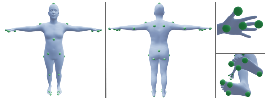
The $K=35$ points (Figure 5) cover the heels, balls and toes of the feet, the palms, fingers and thumbs of the hands, the knees, elbows, shoulders, back, hips, sit bones, sacrum, pelvis, chest and head, each attached to a template vertex with the outward normal of the mesh around it. Point $k$ is described by its signed distance to the scene, read along the normal of the nearest scene point, and by its drift over a window of $0.35$ s spanned by $2h$ frames,

d_{t,k}=\big(\mathbf{v}_{t,k}-\bar{\mathbf{v}}_{t,k}\big)^{\top}\bar{\mathbf{n}}_{t,k},\qquad\xi_{t,k}=\|\mathbf{v}_{t+h,k}-\mathbf{v}_{t-h,k}\|,

(12)

with the distance read on the current body and the drift on the trajectory before any contact term acts on it.

Geometric rule.

A point is a geometric contact when it is near the scene, entering at $d_{t,k}<3$ cm and leaving at $d_{t,k}>3.5$ cm, and still, $\xi_{t,k}<8$ cm.

Physical test.

The geometric rule misses a loaded limb that slides or that the scene cloud does not cover, so we also test whether the motion can be explained without a point. Let $\bm{\tau}^{0}_{t}$ be the root force and moment of Equation 7 evaluated at $\mathbf{f}_{t}=0$ , that is, the wrench that the contacts must provide, and $\mathbf{J}^{\text{r}}_{t,k}$ the root block of the Jacobian of point $k$ . At frozen pose, every candidate point, near the scene or still, receives a force $\mathbf{f}_{t,k}$ in its friction cone $\mathcal{C}_{t,k}$ of Equation 19, and the forces of all candidates solve

\min_{\mathbf{f}_{t,k}\in\mathcal{C}_{t,k}}\;\frac{1}{(mg)^{2}}\Big\|\bm{\tau}^{0}_{t}-\sum_{k}\mathbf{J}^{\text{r}\top}_{t,k}\mathbf{f}_{t,k}\Big\|^{2}+\sum_{k}\pi_{t,k}\,\frac{\|\mathbf{f}_{t,k}\|^{2}}{(mg)^{2}},

(13)

with the moment rows divided by a lever of $0.2$ m, where the price $\pi_{t,k}$ of a point grows with its distance to the scene and with its speed, so that the wrench is explained by the plausible points first. A point is a physical contact when its load enters above 2% of body weight and stays above 1%.

Label.

The label is the union of the two rules, $c^{*}_{t,k}=1$ when either fires, after which spans shorter than $0.1$ s are removed and nearby spans of the same point are merged. Knees are never labeled, since their geometric precision is low, and heels are labeled by geometry only, since a flat foot can route its whole load through the ball. The labels are read on the result of each kinematic pass of Appendix A.3. The first readout is the contact label $c^{*}$ that supervises the model, and the second, $\bar{c}^{*}$ , taken after the pass that pulls each labeled point towards the scene, selects the points that carry a force in the dynamics pass.

A.3 Kinematic objective

The kinematic objective of Equation 8 is a sum of image, prior, smoothness and scene terms,

E_{\text{kin}}(\mathbf{q})=E_{\text{img}}(\mathbf{q})+E_{\text{prior}}(\mathbf{q})+E_{\text{smooth}}(\mathbf{q})+E_{\text{scene}}(\mathbf{q}),

(14)

whose weights in each pass are listed in Table 5. Each sum below is averaged over its active terms, the keypoint term over the sum of the scores, and the weights refer to these averages at 30 fps. The variables are the root translation $\mathbf{r}_{t}$ and the root and joint rotations $\bm{\theta}_{t}$ of every frame, as unit quaternions, with the shape $\bm{\beta}$ frozen.

Image terms.

With $\mathbf{o}_{t,i}(\mathbf{q}_{t})$ the landmarks of the body that the detector sees, $\mathcal{V}(\mathbf{q}_{t})$ its visible mesh vertices, $\operatorname{CD}$ a saturated Chamfer distance and $\rho_{\text{GM}}$ a Geman–McClure kernel that saturates on outliers,

	$\displaystyle E_{\text{img}}(\mathbf{q})=\sum_{t}\Big[$	$\displaystyle w_{\text{init}}\sum_{j}\rho_{\text{GM}}\big(\Pi_{t}(\mathbf{j}_{t,j})-\Pi_{t}(\mathbf{j}^{0}_{t,j})\big)+w_{\text{2D}}\sum_{i}\omega_{t,i}\,\rho_{\text{GM}}\big(\Pi_{t}(\mathbf{o}_{t,i})-\mathbf{y}_{t,i}\big)$		(15)
		$\displaystyle+w_{\text{ch}}\,\operatorname{CD}\big(\mathcal{V}(\mathbf{q}_{t}),\mathcal{P}_{t}\big)\Big].$		(15)

The Chamfer term fixes the depth of the body in the first passes.

Priors.

The pose and orientation priors keep the rotations near the initial estimate through a smooth quaternion distance,

E_{\text{prior}}(\mathbf{q})=\sum_{t}\Big[w_{\text{pose}}\sum_{j\geq 1}\big(1-\langle\bm{\theta}_{t,j},\bm{\theta}^{0}_{t,j}\rangle^{2}\big)+w_{\text{orient}}\big(1-\langle\bm{\theta}_{t,0},\bm{\theta}^{0}_{t,0}\rangle^{2}\big)\Big],

(16)

where $j=0$ is the root, whose translation stays free.

Smoothness.

The smoothness terms act on the second to fourth time differences, which removes the flicker of per-frame estimates while keeping the small movements that load and unload a limb, and a last term penalizes the velocity of each joint along its camera ray $\mathbf{u}_{t,j}$ , the direction that a single view constrains least:

E_{\text{smooth}}(\mathbf{q})=\sum_{t}\Big[\sum_{n=2}^{4}\Big(w^{\text{r}}_{n}\big\|\Delta^{n}(\mathbf{r}_{t},\bm{\theta}_{t,0})\big\|^{2}+w^{\theta}_{n}\sum_{j\geq 1}\big\|\Delta^{n}\bm{\theta}_{t,j}\big\|^{2}\Big)+w_{\text{rad}}\sum_{j}\big(\Delta\mathbf{j}_{t,j}^{\top}\,\mathbf{u}_{t,j}\big)^{2}\Big],

(17)

with the differences of the root pose taken in $\mathfrak{se}(3)$ and those of the joint rotations in $\mathfrak{so}(3)$ .

Scene terms.

The scene terms, a Huber penalty $\rho$ on penetration, an attraction of the labeled points to the nearest surface, an acquisition term and a stillness term, act on the contact points under the current labels $c^{*}_{t,k}$ , provisional in the first pass and those of Appendix A.2 afterwards:

	$\displaystyle E_{\text{scene}}(\mathbf{q})=\sum_{t,k}\Big[$	$\displaystyle w_{\text{pen}}\,\rho\big(\max(0,-d_{t,k})\big)+c^{*}_{t,k}\,w_{\text{att}}\max(0,d_{t,k})$		(18)
		$\displaystyle+c^{}_{t,k}\,w_{\text{acq}}\,\rho_{\delta}\big(\operatorname{dist}(\mathbf{v}_{t,k},\mathcal{Q}_{t,k})\big)+c^{}_{t,k}\,c^{*}_{t+1,k}\,w_{\text{still}}\,\\|\Delta\mathbf{v}_{t,k}\\|^{2}\Big].$		(18)

Acquisition uses the pseudo-Huber kernel $\rho_{\delta}$ of Equation 29, applied to the scalar distance, towards a patch $\mathcal{Q}_{t,k}$ of scene points near the projection of the point, fixed during the fit, which lets the second pass reach a hold that the first pass missed.

Passes.

The optimization runs in four passes with the weights of Table 5. The root pass fits the root alone. The first kinematic pass fits all degrees of freedom with Adam (Kingma and Ba, 2015), with the finger rotations frozen, adds the scene terms under provisional contacts from a looser geometric rule and ends with a few iterations of L-BFGS (Liu and Nocedal, 1989). The second kinematic pass releases the fingers and keeps the scene terms from the start under the labels of Appendix A.2, and the dynamics pass of Appendix A.4 adds the forces.

Table 5: Auto-labeling weights. Terms and weights of Equation 14 to Equation 18 and of Equation 8 and Equation 20 in the root pass, the two kinematic passes and the dynamics pass. Grouped cells list the weights of the second, third and fourth differences for smoothness, of the first to third differences for the forces and of the first and second for the torques.

Term	Weight	Root	Pass 1	Pass 2	Dynamics
Reprojection to the initial joints	$w_{\text{init}}$	30	30	30	30
Reprojection to the Sapiens2 keypoints	$w_{\text{2D}}$	8	8	8	8
Chamfer distance to the human depth cloud	$w_{\text{ch}}$	10	10	0	0
Pose prior	$w_{\text{pose}}$	300	300	300	300
Root orientation prior	$w_{\text{orient}}$	50	50	50	50
Smoothness of the root pose	$w^{\text{r}}_{n}$	24 / 300 / 300	400 / 300 / 300	24 / 300 / 300	24 / 300 / 300
Smoothness of the joint rotations	$w^{\theta}_{n}$	48 / 500 / 500	800 / 500 / 500	48 / 500 / 500	48 / 500 / 500
Radial velocity along the camera ray	$w_{\text{rad}}$	0	400	100	100
Penetration	$w_{\text{pen}}$	0	12000	12000	12000
Contact attraction	$w_{\text{att}}$	0	10	0	20
Contact acquisition	$w_{\text{acq}}$	0	0	1000	0
Contact stillness	$w_{\text{still}}$	0	500	4000	4000
Root wrench, force / moment	$w_{F}$ / $w_{T}$	–	–	–	50 / 300
Joint torques, scaled by $\mu_{j}$	$w_{J}$	–	–	–	30
Force magnitude	$w_{\text{mag}}$	–	–	–	1
Force smoothness	$w^{\Delta f}_{n}$	–	–	–	120 / 640 / 400
Torque smoothness	$w^{\Delta\tau}_{n}$	–	–	–	8 / 30

A.4 Force model and dynamics pass

Multibody.

The body of Equation 7 has 52 segments, one per SMPL-X joint except the jaw and eyes, whose parts are merged into the head, whose masses and inertias are integrated from the shaped mesh as in PhysPT (Zhang et al., 2024) with the tissue densities of Dempster (1955), and $m$ is their sum. The velocities $\dot{\mathbf{q}}_{t}$ and accelerations $\ddot{\mathbf{q}}_{t}$ are central differences on the manifold, and gravity points along the estimated down direction of Appendix A.6. Over the corpus the estimated mass averages 64 kg (46 to 86 kg), and on ForceWall it is 62.2 kg for the 72.5 kg climber and 51.5 kg for the 48 kg climber, which we attribute to a shape estimator that compresses towards the mean of its training population.

Friction cone.

Each force lives on its contact point and is restricted to a pyramidal friction cone of half-angle $45^{\circ}$ about the inward normal $-\mathbf{n}_{t,k}$ , spanned by four edges $\mathbf{e}_{t,k,\nu}$ with non-negative coefficients,

\mathbf{f}_{t,k}\in\bar{c}^{*}_{t,k}\,\mathcal{C}_{t,k},\qquad\mathcal{C}_{t,k}=\Big\{\sum_{\nu=1}^{4}a_{\nu}\,\mathbf{e}_{t,k,\nu}:a_{\nu}\geq 0\Big\},

(19)

with the edges evaluated at the pose that starts the pass and held fixed, so that the body cannot rotate to make a force cheap. The force enters Equation 7 through the Jacobian of its point, as a force and a lever moment on the parent joint, so that moving the body changes the physics.

Regularizer.

The term $E_{\text{reg}}$ of Equation 8 penalizes the magnitude of each force, its first three time differences and the first two time differences of the joint torques,

E_{\text{reg}}(\mathbf{q},\mathbf{f})=\sum_{t,k}\Big[w_{\text{mag}}\frac{\|\mathbf{f}_{t,k}\|^{2}}{(mg)^{2}}+\sum_{n=1}^{3}w^{\Delta f}_{n}\frac{\|\Delta^{n}\mathbf{f}_{t,k}\|^{2}}{(mg)^{2}}\Big]+\sum_{t,j}\sum_{n=1}^{2}w^{\Delta\tau}_{n}\frac{(\Delta^{n}\tau_{t,j})^{2}}{(mg\ell)^{2}},

(20)

where a force difference is taken only where the contact persists over its stencil, with half the weight on the component across the mean direction of the force, so that a force may turn more freely than it may change magnitude.

Torque multipliers.

Table 6 gives the multipliers $\mu_{j}$ of the joint-torque term, 200 N m divided by an approximate maximum voluntary torque of each joint group (Anderson et al., 2007; Holzbaur et al., 2007; Delp et al., 1996). This term resolves the split of the load between limbs that the root wrench alone leaves undetermined: a load that the body could carry with either limb goes where the weighted torque is cheapest. Climbers are stronger in the fingers than the population these numbers describe, so the values are coarse.

Table 6: Torque multipliers. The multipliers

\mu_{j}

per joint group and the maximum voluntary torque they encode.

	hip, knee, spine	ankle, foot	neck, head	collar, shoulder	elbow	wrist	fingers
Max. torque [N m]	200	118	33	80	61	12	8
$\mu_{j}$	1.0	1.7	6.0	2.5	3.3	17	25

Solver.

The dynamics pass first solves the cone coefficients $a_{\nu}$ with L-BFGS at the frozen pose of the second kinematic pass, then pose and forces jointly with the kinematic terms of Equation 14 still active, which gives $\mathbf{q}^{*}$ and $\mathbf{f}^{*}$ . The labeled force $\mathbf{f}^{*}_{t,k}$ is stored in the world in newtons and, for training, converted to units of body weight in the body frame of the input trajectory $\mathbf{q}_{t}$ (Appendix B.6).

A.5 Label confidences

The contact confidence $w^{\text{c}}_{t,k}$ is a logistic function of the log drift $\xi_{t,k}$ of the point over the stillness window and of the log time to the nearest change of its label, with one intercept per body part and separate coefficients for contact and free labels. The force confidence of a frame is

w^{\text{f}}_{t}=\psi(\epsilon^{f}_{t})\,\psi(\epsilon^{m}_{t})\,\psi(\epsilon^{o}_{t}),\qquad\psi(x)=\frac{1}{1+(x/x_{0})^{2}},

(21)

where $\epsilon^{f}_{t}=\|\bm{\tau}^{f}_{t}\|/(mg)$ and $\epsilon^{m}_{t}=\|\bm{\tau}^{m}_{t}\|/(mg\cdot 0.2\,\text{m})$ are the residual root force and moment of Equation 7 at $(\mathbf{q}^{*},\mathbf{f}^{*})$ , $\epsilon^{o}_{t}$ the excess of the summed force magnitudes over three body weights, in body weights, and $x_{0}=0.5$ , $1.5$ and $1.0$ respectively.

A.6 Gravity

GeoCalib (Veicht et al., 2024) runs on 48 frames, and its camera-frame up vectors are lifted to the world with the VGGT- $\Omega$ rotations and averaged after inlier selection at $8^{\circ}$ . The estimate is accepted when the cameras span at least $8^{\circ}$ of rotation and the votes spread less than $5^{\circ}$ . Otherwise a RANSAC plane through the lowest fused points gives the down direction, and failing that the down axis of the first camera. Only the direction is estimated.

A.7 BEDLAM2

We import every BEDLAM2 (Tesch et al., 2025) sequence whose bodies all have a released motion in the AMASS format (Mahmood et al., 2019), excluding the egocentric and upper-body render jobs and the sequences flagged as test set, with the ground-truth SMPL-X (Pavlakos et al., 2019) bodies, cameras and the floor height of each sequence. The shape is truncated to 10 coefficients, a frame is valid when the person is visible, and the person masks $\mathbf{s}_{t}$ that the backbone needs are rasterized from the ground-truth meshes.

With the ground-truth trajectory and cameras, no perception model runs and the contact rule of Appendix A.2 is replaced by a near-and-still rule against the floor plane of the sequence. A point is in contact when it is below 8 cm above the floor, leaving at 10 cm, faces down to within $55^{\circ}$ , stays for at least $0.1$ s and moves slower than $0.2$ m/s, the speed being the calmer of its means over the preceding and the following $0.1$ s. The forces are then solved at the frozen ground-truth pose with the dynamics terms of Equation 8 and Equation 20, plus a ramp term that penalizes the force on the first and last frame of each contact, weakened by $1/(1+(v/0.8\,\text{m/s})^{2})$ with $v$ the vertical speed of the root, so that loads ramp in and out unless the body is moving fast. The contact and force confidences are set to one.

A.8 Benchmarks

On ForceWall, the parkour sequences and OpenCap the camera is static, so the pipeline uses the scale of Equation 11 without the refinement. On ForceWall and the parkour sequences it drops the Chamfer term and restricts the contact points to the 18 of the hands and feet, and on the parkour footage the scene terms are disabled. On OpenCap the scene is a plane fitted to the floor, with the chair and the box detected as plateaus, the contact points are the ten of the feet and the two sit bones, the ramp term of Appendix A.7 is added, and the measured mass is given to the solver for the true-mass columns of Table 13.

Appendix B Model and training details

This appendix details the architecture of Section 3.1 and the losses of Section 3.2.2, following their notation.

B.1 Contact-force tokens

The $K=35$ input embeddings $\mathbf{z}_{t}=(\mathbf{z}_{t,k})_{k=1}^{K}$ of Equation 2 are learned vectors of width 1024, one per contact point of Figure 5, appended after the original token sequence of the six-layer SAM 3D Body decoder. The attention mask is asymmetric: the original tokens do not attend to the appended ones, so the pose token $\mathbf{p}_{t}$ and the readout of the backbone are unchanged. After each of the first five decoder layers, token $k$ adds a linear projection of the backbone features sampled on a $5\times 5$ grid around the current projection of its point, located through the intermediate body readout of the decoder, together with a positional embedding of that projection. The outputs $\mathbf{z}^{\prime}_{t}$ are the appended tokens after the last layer.

B.2 Body and camera heads

The heads $\mathcal{H}_{\mathrm{SMPL\text{-}X}}$ and $\mathcal{H}_{\mathrm{camera}}$ of Equation 1 are two feed-forward branches on the final pose token, of the same shape as the SAM 3D Body heads. The first regresses the root and 21 body rotations and 30 finger rotations in 6D form and the 10 shape parameters, as residuals on a mean body, and the second a weak-perspective camera $\bm{\kappa}_{t}$ that CLIFF (Li et al., 2022b) lifts to the full-frame translation $\mathbf{r}^{c}_{t}$ with the crop box and the focal length.

B.3 World-informed pose token

The kinematics that enter $\operatorname{MLP}_{\mathrm{world}}$ in Equation 3 are the joint positions and velocities of the world trajectory re-expressed in the body frame of frame $t$ , so that nothing depends on the orientation of the world frame. They comprise the joint positions and the joint rotations in 6D form, the backward and forward angular rates of the joints, the backward and forward linear and angular velocities of the root, the frame spacing, the clip-mean shape $\bm{\beta}$ , and the direction, distance, bearing, size and axes of the camera, 351 channels in all. In practice $\operatorname{MLP}_{\mathrm{world}}$ is a layer normalization of these channels and $\operatorname{MLP}_{\mathrm{pose}}$ a linear projection of $\mathbf{p}_{t}$ to 256 channels, and their concatenation $\mathbf{p}^{\prime}_{t}$ is projected to width 512 by one linear layer. The contact-force tokens $\mathbf{z}^{\prime}_{t,k}$ are projected to the same width, and a learned embedding tells the $K+1$ slots apart.

B.4 Temporal transformer and iterative refinement

The transformer $\mathcal{T}$ of Equation 4 has three pre-norm blocks of width 512 with 8 heads, a feed-forward ratio of 4 and dropout $0.1$ . In each block, attention runs first along time within every slot, with rotary embeddings (Su et al., 2024) on elapsed time and masked to $\pm 0.083$ s, then across the $K+1$ slots within a frame, followed by the feed-forward layer. Three blocks give a receptive field of $\pm 0.25$ s, so the model trained on 120-frame windows is applied to whole videos, resampled to about 25 fps, in windows of 240 frames overlapping by 120.

The three blocks $\mathcal{T}_{1},\mathcal{T}_{2},\mathcal{T}_{3}$ are applied one at a time, and the pose is corrected after each of them, which is the iterative refinement of Section 3.1.2. With $(\mathbf{p}^{(0)}_{t},\mathbf{z}^{(0)}_{t})=(\mathbf{p}^{\prime}_{t},\mathbf{z}^{\prime}_{t})$ and $\hat{\mathbf{q}}^{(0)}_{t}=\mathbf{q}_{t}$ , block $i$ computes

(\mathbf{p}^{(i)}_{t},\mathbf{z}^{(i)}_{t})_{t=1}^{T}=\mathcal{T}_{i}\big((\mathbf{p}^{(i-1)}_{t},\mathbf{z}^{(i-1)}_{t})_{t=1}^{T}\big),\qquad\hat{\mathbf{q}}^{(i)}_{t}=\hat{\mathbf{q}}^{(i-1)}_{t}\oplus\mathcal{H}_{\mathrm{offset}}(\mathbf{p}^{(i)}_{t}),

(22)

after which the body model is re-run in the world with the clip-mean shape and the contact, force and gravity heads are read from $(\mathbf{p}^{(i)}_{t},\mathbf{z}^{(i)}_{t})$ . The refresh of Equation 3 before the next block is a residual update of the pose token with the recomputed kinematics and the current predictions,

\mathbf{p}^{(i)}_{t}\leftarrow\mathbf{p}^{(i)}_{t}+\mathbf{W}_{\text{fb}}\,\operatorname{LN}\big(\mathbf{j}_{t}(\hat{\mathbf{q}}^{(i)}),\,\dot{\mathbf{j}}_{t}(\hat{\mathbf{q}}^{(i)}),\,\hat{\mathbf{c}}^{(i)}_{t},\,\mathbf{R}_{t}^{\top}\hat{\mathbf{g}}^{(i)}\big),

(23)

with $\mathbf{W}_{\text{fb}}$ a zero-initialized linear layer and $\hat{\mathbf{g}}^{(i)}$ the clip gravity estimate of Appendix B.5, rotated into the body frame of frame $t$ by the root orientation $\mathbf{R}_{t}$ . The outputs of Equation 4 are those of the last block, $(\mathbf{p}^{\prime\prime}_{t},\mathbf{z}^{\prime\prime}_{t})=(\mathbf{p}^{(3)}_{t},\mathbf{z}^{(3)}_{t})$ and $\hat{\mathbf{q}}_{t}=\hat{\mathbf{q}}^{(3)}_{t}$ , and the contact, force, trajectory and gravity losses are also applied to the predictions of the first two blocks at weight $0.5$ . The trainable part has 19.7M parameters on top of the 1.3B frozen backbone and decoder.

B.5 Prediction heads

The heads $\mathcal{H}_{\mathrm{contacts}}$ , $\mathcal{H}_{\mathrm{force}}$ and $\mathcal{H}_{\mathrm{offset}}$ of Equation 5 and Equation 6 are two-layer MLPs with GELU, shared across the three blocks. The offset head yields 6D corrections of the root and the 21 body joints and a root shift in the body frame, and the finger rotations are left as predicted per frame. The force head regresses $\tilde{\mathbf{f}}_{t,k}$ in the body frame of frame $t$ and in units of body weight, and the gated world force in newtons of Equation 5 is

\hat{\mathbf{f}}_{t,k}=\hat{c}_{t,k}\,mg\,\mathbf{R}_{t}\,\tilde{\mathbf{f}}_{t,k},

(24)

with $\mathbf{R}_{t}$ the root orientation of the input trajectory $\mathbf{q}_{t}$ and $m$ the mass of the reconstructed body. The gravity head of Equation 6 predicts from $\mathbf{p}^{\prime\prime}_{t}$ a per-frame vote for the down axis, as a correction of the down axis of the camera, and the unit votes are averaged over the clip and renormalized into the gravity direction $\hat{\mathbf{g}}$ .

B.6 Losses

Table 7 lists the terms and weights. The labels are the trajectory $\mathbf{q}^{*}$ , the contacts $c^{*}_{t,k}$ and the forces $\mathbf{f}^{*}_{t,k}$ of Equation 8, with the confidences $w^{\text{c}}_{t,k}$ and $w^{\text{f}}_{t}$ of Appendix A.5, and $\rho$ denotes the Huber loss of Equation 9 with the scale given in Table 7.

Table 7: Training losses. Terms and weights. Confidence-weighted terms are marked in the last column, and the contact, force, trajectory and gravity terms also supervise the intermediate blocks at weight 0.5. Huber losses are given with their scale.

Loss	Definition	Weight	Conf.
Per-frame body $\mathcal{L}_{\text{body}}$ (SMPL-X and camera heads)
2D joints	Huber on the full-frame projection, crop units, $\delta=0.05$	10
3D joints	Huber, pelvis-relative, $\delta=0.1$ m	5
Root, body and finger rotations	squared error on 6D	1, 1, 0.5
Shape	squared error	0.1
Camera	Huber on the weak-perspective parameters, $\delta=0.05$	1
Corrected trajectory $\mathcal{L}_{\text{traj}}$ (offset head)
3D joints, rotations	as above	10, 2
World root	clip mean ( $\delta=0.1$ m), per-frame deviation ( $\delta=0.02$ m)	2, 2
Joint velocity, root angular velocity	Huber on forward differences, scaled by 0.4 m/s and 0.57 rad/s	1, 1
Contacts $\mathcal{L}_{\text{c}}$	binary cross-entropy, per point	35/6	$\checkmark$
Force vector $\mathcal{L}_{\text{f}}$ , magnitude $\mathcal{L}_{\text{mag}}$	Huber, $\delta=0.5$ bw, on labeled contacts	1, 1	$\checkmark$
Force off contact (in $\mathcal{L}_{\text{f}}$ )	$L_{1}$ on the magnitude	1	$\checkmark$
Net force $\mathcal{L}_{\text{net}}$	Huber on the sum over points	1	$\checkmark$
Contact stillness $\mathcal{L}_{\text{still}}$	$L_{1}$ on the world speed of a labeled contact	1	$\checkmark$
Gravity $\mathcal{L}_{\text{g}}$	$1-\cos$ , scenes with an accepted gravity estimate	5
Physics $\mathcal{L}_{\text{phys}}$	$\lambda_{F}=5$ , $\delta_{F}=0.2$ ; $\lambda_{T}=20$ , $\delta_{T}=0.5$ ; $\lambda_{J}=0.3$

Per-frame body.

The heads of Appendix B.2 are trained as in HMR 2.0 (Goel et al., 2023) against the labels projected into the camera, with Huber losses on the full-frame projection of the joints, on the pelvis-relative 3D joints and on the weak-perspective camera, squared errors on the rotations in 6D form and on the shape, and the finger joints weighted $0.1$ .

Corrected trajectory.

The corrected trajectory $\hat{\mathbf{q}}$ of Equation 6 is supervised on its pelvis-relative joints and rotations, on its world root and on the velocities of its joints and of its root orientation:

$\displaystyle\mathcal{L}_{\text{traj}}=\sum_{t}\Big[$	$\displaystyle\lambda_{\text{j}}\,\rho\big(\mathbf{j}_{t}(\hat{\mathbf{q}})-\mathbf{j}_{t}(\mathbf{q}^{})\big)+\lambda_{\theta}^{\prime}\big\\|\hat{\bm{\theta}}_{t}-\bm{\theta}^{}_{t}\big\\|^{2}$	(25)
	$\displaystyle+\lambda_{\text{v}}\,\rho\Big(\frac{\Delta\mathbf{j}_{t}(\hat{\mathbf{q}})-\Delta\mathbf{j}_{t}(\mathbf{q}^{})}{\Delta t}\Big)+\lambda_{\omega}\,\rho\Big(\frac{\Delta\hat{\bm{\theta}}_{t,0}-\Delta\bm{\theta}^{}_{t,0}}{\Delta t}\Big)\Big]$
	$\displaystyle+\lambda_{\text{r}}\,\rho\big(\bar{\mathbf{e}}\big)+\lambda_{\text{r}}^{\prime}\sum_{t}\rho\big(\hat{\mathbf{r}}_{t}-\mathbf{r}^{}_{t}-\bar{\mathbf{e}}\big),\qquad\bar{\mathbf{e}}=\frac{1}{T}\sum_{t}\big(\hat{\mathbf{r}}_{t}-\mathbf{r}^{}_{t}\big),$

where the rotations of the body joints are compared in 6D form and the differences of the root orientation are taken in $\mathfrak{so}(3)$ . The root translation is scored on the clip-mean error $\bar{\mathbf{e}}$ and on the per-frame deviation from it, since the scale of a monocular reconstruction is uncertain as a whole.

Contacts and forces.

The contact loss $\mathcal{L}_{\text{c}}$ of Equation 9 is normalized per point before summing, so that the rare points weigh as much as the frequent ones. The forces $\tilde{\mathbf{f}}_{t,k}$ and $\mathbf{f}^{*}_{t,k}$ of Equation 9 are compared in the body frame of the input trajectory $\mathbf{q}_{t}$ , into which the label is rotated, in units of body weight, and $\mathcal{L}_{\text{f}}$ is complemented by a term on the magnitude of each labeled force and by one on the net force over the points,

\mathcal{L}_{\text{mag}}=\sum_{t,k}w^{\text{f}}_{t}\,\bar{c}^{*}_{t,k}\,\rho\big(\|\tilde{\mathbf{f}}_{t,k}\|-\|\mathbf{f}^{*}_{t,k}\|\big),\qquad\mathcal{L}_{\text{net}}=\sum_{t}w^{\text{f}}_{t}\,\rho\Big(\sum_{k}\tilde{\mathbf{f}}_{t,k}-\sum_{k}\mathbf{f}^{*}_{t,k}\Big),

(26)

which ties the sum of the predictions to the sum of the labels even when the split between points is uncertain. Contact points whose labeled force exceeds four body weights, a sign of a wrong scale or camera, are excluded from the force losses.

Contact stillness.

A point labeled in contact should not move in the world, so the corrected trajectory is penalized on the speed of its labeled contacts,

\mathcal{L}_{\text{still}}=\sum_{t,k}w^{\text{c}}_{t,k}\,c^{*}_{t,k}\,\frac{\|\Delta\mathbf{v}_{t,k}(\hat{\mathbf{q}})\|}{\Delta t},

(27)

with $\mathbf{v}_{t,k}(\hat{\mathbf{q}})$ the world position of contact point $k$ on the corrected body.

Gravity.

With $\mathbf{g}^{*}$ the scene gravity of Appendix A.6, $\mathcal{L}_{\text{g}}=1-\hat{\mathbf{g}}^{\top}\mathbf{g}^{*}$ per clip on the scenes whose GeoCalib estimate is accepted.

B.7 Physics loss

The physics loss of Equation 10 evaluates Equation 7 on the corrected trajectory $\hat{\mathbf{q}}$ with the predicted forces. The body is the multibody of Appendix A.4 reduced to the 22 body joints, with the finger parts merged into the hand segments and masses and inertias integrated from the clip-mean shaped mesh, the velocities and accelerations are central differences on the manifold with a $\pm 2$ -frame stencil for the acceleration, and gravity is the estimate $\mathbf{g}^{*}$ of the scene (Appendix A.6). Each predicted force enters in world newtons as in Equation 24 with its gate detached,

	$\displaystyle\hat{\mathbf{f}}_{t,k}$	$\displaystyle=\operatorname{sg}\big(\hat{c}_{t,k}\big)\,mg\,\mathbf{R}_{t}\,\tilde{\mathbf{f}}_{t,k},$		(28)
	$\displaystyle\bm{\tau}_{t}$	$\displaystyle=\mathbf{M}(\hat{\mathbf{q}}_{t})\,\ddot{\hat{\mathbf{q}}}_{t}+\mathbf{b}(\hat{\mathbf{q}}_{t},\dot{\hat{\mathbf{q}}}_{t})+\mathbf{G}(\hat{\mathbf{q}}_{t})-\mathbf{J}(\hat{\mathbf{q}}_{t})^{\top}\hat{\mathbf{f}}_{t},$		(28)

where $\operatorname{sg}$ is the stop-gradient and $\mathbf{J}(\hat{\mathbf{q}}_{t})$ the Jacobian of the contact points, so that each force acts at its point $\mathbf{v}_{t,k}(\hat{\mathbf{q}})$ and produces a lever moment on its parent joint. Detaching the gate keeps the contact probabilities from being driven by the physics, which would let the model switch a contact off to cancel a residual. The root force and moment $\bm{\tau}^{f}_{t}$ and $\bm{\tau}^{m}_{t}$ of the result are the residual that the forces fail to explain and enter Equation 10 through the pseudo-Huber loss

\rho_{\delta}(\mathbf{e})=\frac{1}{3}\sum_{i=1}^{3}\delta^{2}\Big(\sqrt{1+e_{i}^{2}/\delta^{2}}-1\Big),

(29)

applied per component, which is quadratic on small residuals and linear on the large ones that a wrong label or a missed contact produces. The joint-torque term of Equation 10 uses the multipliers $\mu_{j}$ of Table 6 without the fingers, which the corrected trajectory does not move, and acts on the forces only, the body being detached in that term, so that it distributes the load between limbs without pulling on the pose. The loss is averaged over the frames whose stencil is valid and backpropagates into the force head and, through the root terms, into the offset head.

B.8 Training

Clips are 120 frames, resampled to about 25 fps for ClimbingVideos with a random offset per epoch and at 30 fps for BEDLAM2, with no other augmentation. All runs use AdamW with weight decay $0.01$ , a cosine schedule to $10^{-6}$ and an exponential moving average of the weights, which is what we evaluate. The ClimbingVideos model trains for 10 epochs at learning rate $3\times 10^{-4}$ with 300 warm-up steps and 32 clips per step, and the BEDLAM2 model with the same schedule on a fresh random third of the sequences per epoch with 24 clips per step. The joint model starts from the BEDLAM2 model and trains for 5 epochs at learning rate $10^{-4}$ without warm-up on 16 ClimbingVideos and 16 BEDLAM2 clips per step, one pass over ClimbingVideos per epoch and a fresh 7% of BEDLAM2. Each ablation rung of Table 4 is trained from scratch with the ClimbingVideos schedule, and the last checkpoint of every run is reported.

Appendix C Datasets and metrics

Table 8 summarizes the data and Table 9 the curation of ClimbingVideos. Contacts are scored on every dataset by precision, recall and F1 at threshold $0.5$ , without temporal tolerance, micro-averaged over frames and limbs. The $K$ predicted probabilities are folded to a limb $b$ by their maximum, $\hat{c}_{t,b}=\max_{k\in b}\hat{c}_{t,k}$ . Per-vertex estimators are folded to the limbs by the skinning weights or the part segmentation of the vertices, either any contact vertex or a tenth of them, and the best of the four rules is reported on ClimbingVideos and ForceWall, while on RICH the predictions are folded by the rule of its labels (Appendix C.3). GVHMR and PromptHMR report their stationary-joint probabilities at $0.5$ .

Table 8: Datasets. Data used in this paper.

	Sources	Scenes	Frames	Labels
ClimbingVideos train	149	1,419	460k	pseudo
ClimbingVideos test	42	109	31k	pseudo, manual contacts
BEDLAM2 (Tesch et al., 2025)	59 jobs	18,076	5.5M	true pose, pseudo contacts and forces
ForceWall	14	68	29.6k	sensors, multi-view pose
RICH (Huang et al., 2022)	8 subjects	164	70.2k	contact labels
Parkour (Li et al., 2019)	–	28	2.3k	motion capture, plates and bar
OpenCap (Uhlrich et al., 2023)	9 subjects	64	–	force plates

Table 9: Curation funnel. Curation of ClimbingVideos. Counts are YouTube videos until the scene split and scenes afterwards.

Stage	Count
Videos returned by keyword search (“bouldering gym”, “moonboard climbing” and the like)	782
Duration between 10 s and 20 min	591
Thumbnail and metadata VLM gate	584
Downloaded at up to 1080p (48 h of video)	581
Scenes after shot detection, between 100 and 500 frames	16,152
Full-body pose gate: in half of the sampled frames, a person with 60% of the 17 COCO keypoints visible, including an ankle, a shoulder and a hip, spanning 40% of the frame height	4,612
Video VLM gate: moving climber, single real-time shot	3,738
Indoor and not rope-supported	3,071
Manual selection (from 191 videos)	1,528

C.1 ClimbingVideos

Curation.

The gates and their thresholds are listed in Table 9. Shots are detected with a content-change detector, long scenes are split uniformly, and a boundary guard removes frames leaking from a neighboring shot. The full-body gate runs a YOLO pose detector (Jocher et al., 2026) on every fifth frame, and the video VLM (Clark et al., 2026) answers a fixed rubric, including the type of climbing and whether a rope carries the climber’s weight, on 24 uniformly sampled frames. The climber it points at is associated with a track of BoT-SORT (Aharon et al., 2022) on top of the pose detector.

Statistics.

The selected scenes (Figure 6) have a mean length of 322 frames (10.7 s), 92% are 1080p, and the source frame rate is 24 to 60 fps with a median of 25. The split is by source video, with the test scenes drawn from videos with at most four scenes.

Contact labels and scoring.

The test split carries a contact label (in contact, free or unknown) for 14 joints on its 31k frames, made with the tool of Figure 7. Hands are in contact in 84% of the frames, toes in 63%, heels in 8%, and knees, elbows, shoulders and hips in less than 2%. Contacts are scored on six limbs, the two hands, the two toes and the two heels, to which the annotated hand, toe and heel labels are folded, and the 17 points outside them are not scored.

C.2 ForceWall

Hardware.

The wall (Figure 8) has four instrumented panels of 0.6 $\times$ 1.1 m, the quarters of a bouldering board, so that in normal climbing each limb loads one panel and a sensor channel is the force of one limb. Each panel rests on three custom three-axis load cells, each built from six single-point load cells (CZL635, Phidgets), sampled at 100 Hz through an amplifier. The panels were calibrated along each axis with known loads, with an accuracy of at least 95% and a crosstalk of at most 5%. The frame is tilted to $0^{\circ}$ , $16^{\circ}$ or $32^{\circ}$ , and the holds mounted on the panels elicit side pulls, underclings, pockets and crimps for the hands as well as heel hooks, knee drops and flagging.

Recording.

Two participants, one male (72.5 kg, 1.80 m) and one female (48 kg, 1.60 m), perform bouldering movements in a self-chosen order, recorded at 30 fps and 1080p by three webcams (C920, Logitech), two behind the participant at different angles and one lateral, and cut into clips of at most 500 frames. Forces are debiased on a quiet stretch and mapped to the world with the sensor datasheet and the wall’s azimuth from the reconstructed scene. The sensors and the three cameras are synchronized on the first loading of the left hand and on the reprojection error of the stereo fit. Ground-truth contact is a load above 50 N entering and 30 N leaving, scored on the four limbs, a foot being in contact when its toes or its heel are.

Reference pose.

The multi-view reference pose is fitted with the optimization of Appendix A with three changes. The reprojection terms act in all three cameras, calibrated with a chessboard (0.2 to 0.3 px reprojection error), the SMPL-X shape of each climber is fitted once against the true height and weight and then frozen, and the measured contacts and forces enter as constraints, the latter through a term that pulls the sum of the point forces of each limb to its sensor. The fit is seeded in every view by SAM 3D Body, and 29.6k of its frames are valid and scored. Pose is scored by MPJPE on the 22 body joints after hip centering in the camera frame.

Force metrics.

The predicted forces are summed by limb $b$ , $\hat{\mathbf{F}}_{t,b}=\sum_{k\in b}\hat{\mathbf{f}}_{t,k}$ , in newtons with the mass $m$ that our pipeline reconstructs for the clip (the baselines keep the mass of their own body model, Appendix C.6). They are compared with the sensor force $\mathbf{F}_{t,b}$ on the set $\mathcal{S}$ of limb-frames $(t,b)$ with a valid reference, in contact or not, so that force leaked onto a free limb is penalized:

\text{MAE}=\frac{1}{|\mathcal{S}|}\sum_{(t,b)\in\mathcal{S}}\big\|\hat{\mathbf{F}}_{t,b}-\mathbf{F}_{t,b}\big\|.

(30)

The angle is the mean of $\arccos\big(\hat{\mathbf{F}}_{t,b}^{\top}\mathbf{F}_{t,b}/(\|\hat{\mathbf{F}}_{t,b}\|\|\mathbf{F}_{t,b}\|)\big)$ over the limb-frames where both magnitudes exceed 50 N, and the correlation is the Pearson correlation of the magnitudes $\|\hat{\mathbf{F}}_{t,b}\|$ and $\|\mathbf{F}_{t,b}\|$ pooled over frames and limbs. The load-share error is the mean absolute difference, in percentage points, between the predicted share $\|\hat{\mathbf{F}}_{t,b}\|/\sum_{b^{\prime}}\|\hat{\mathbf{F}}_{t,b^{\prime}}\|$ of a limb and the measured share $\|\mathbf{F}_{t,b}\|/\sum_{b^{\prime}}\|\mathbf{F}_{t,b^{\prime}}\|$ . The physical residual is the mean of $\|\bm{\tau}^{f}_{t}\|/(mg)$ and of $\|\bm{\tau}^{m}_{t}\|/(mg)$ with the root wrench of Equation 28, that is, with the forces gated by the contact probabilities, in body weights (bw) and body weights times meters.

C.3 RICH

We score the static-camera sequences of the RICH (Huang et al., 2022) test split on the frames of the contact evaluation of BSTRO, excluding the two-person sequences: 164 clips, one per sequence, camera and subject, with 70,159 frames of 8 subjects in three scenes. The per-vertex labels of RICH are folded to the six limbs of Appendix C.1 through the SMPL joint with the largest skinning weight of each vertex, the hands from the wrist and hand joints, the toes from the foot joint and the heels from the ankle joint, and a limb is in contact when at least one of its vertices is labeled. Every method receives the ground-truth person box, our model and PromptHMR also the ground-truth silhouette as the mask, and the video models run on the full timeline of each sequence and are scored on the annotated frames only. The per-vertex predictions of BSTRO, DECO and InteractVLM are thresholded at $0.5$ and folded by the same rule.

C.4 Parkour

The 28 sequences of Li et al. (2019) are archival PAL footage (720 $\times$ 576, 25 fps) with Vicon motion capture on 16 joints and contact forces measured by force plates under the feet and an instrumented bar under the hands, 2,324 reference frames in all. We score every method with the evaluator shipped with the dataset, against the original force files of the authors, and convert every method’s forces to newtons with the 74.6 kg body that the evaluator assumes, so that no method is favored by its mass estimate. The evaluator aligns each frame to the 16 Vicon joints by a similarity transform and reports the mean joint error, and scores the summed force of each limb against the plates and the bar by the mean norm of the vector difference over the frames of a clip, averaged over clips.

C.5 OpenCap

The validation set of Uhlrich et al. (2023) was recorded with smartphones on nine subjects walking, squatting, rising from a chair and dropping from a box over force plates. We take one camera and the natural-speed trials, exclude six whose synchronization with the plates we could not verify, and score the remaining 64, of which 22 walking trials of eight subjects form the walking subset. The forces of every method and the plates are filtered with a fourth-order zero-lag Butterworth filter, at 6 Hz for walking and 4 Hz for squats and sit-to-stand, with the drop jumps unfiltered. The vertical, anteroposterior and mediolateral errors of each foot, in percent of body weight, are averaged over the frames of a trial, then over the trials of a subject, then over subjects. Over the four activities every frame on which the plates watched a foot counts, the protocol of Uhlrich et al. (2023), and on walking only the stance frames, where the plate reads more than 5% of body weight, the protocol of Gilon et al. (2026), whose numbers are taken from their paper. Every method that estimates its own mass is scored twice, with its forces in its own newtons and with them rescaled by the ratio of the measured to its estimated mass, which gives the true-mass columns of Table 3 and Table 13, except for our optimization, where the measured mass is given to the solver.

C.6 Baselines

Li et al. (2019)++.

We run the released estimator of Li et al. (2019) with our inputs in place of its own: the per-frame SAM 3D Body body as the initial pose, with the SMPL shape fitted to its skeleton, the Sapiens2 keypoints folded to the OpenPose joints, and its own contact recognizer applied to those keypoints. On ForceWall the method also receives the calibrated camera and the gravity direction of our pipeline, fits its ground plane through the feet in contact and frees the plane in its last stage, and the hands hold a virtual object as in the original method.

PhysPT.

We run the released PhysPT (Zhang et al., 2024) with its checkpoints on the per-frame SAM 3D Body poses in place of its CLIFF input, without translation, which PhysPT predicts itself. Its per-vertex ground reaction forces are summed per foot and placed at their force-weighted centroid, a foot counts as in contact above 20 N, and the hands never carry force. PhysPT leaves the last frame of every clip unpredicted, which is excluded on ForceWall and counts as zero force on the parkour sequences.

Inverse dynamics.

The per-frame SAM 3D Body poses are smoothed with a Gaussian of $0.1$ s, and the contacts are the InteractVLM (“wall”) vertex probabilities folded to the limbs, a limb being in contact when a tenth of its vertices exceed the threshold. One force per limb in contact, acting at the wrist or at the base of the toes, solves the six root-wrench equations of Equation 7 per frame in the least-squares sense, without friction cone, joint torque or smoothness.

Units.

On ForceWall our forces and those of the inverse dynamics are converted to newtons with the mass that our pipeline reconstructs for the clip, Li et al. (2019)++ and PhysPT keep the newtons of their own body models, and on the parkour sequences every method is rescaled to the 74.6 kg body of the evaluator (Appendix C.4).

Appendix D Limitations and future work

PACT models the interaction between a person and a rigid, static scene, with three simplifications. First, hand-held objects are not represented, so neither the pipeline nor the model accounts for their forces, which leaves lifting, carrying and tool use out of scope. Retrieving the objects and adding their dynamics to the optimization of Section 3.2.1 would extend the labels, and the model, to these interactions. Second, every support is assumed rigid, so mats, ropes or trampolines, whose forces depend on their deformation, are out of reach, and the method is restricted to activities on rigid ground and structures. Third, the body is the articulated rigid body of SMPL-X with the segments of Appendix A.4, and we estimate contact forces rather than the muscle forces that produce them. Muscle estimation is a separate problem that requires a musculoskeletal body, for which a biomechanically accurate skeleton such as SKEL (Keller et al., 2023) is a natural step, although few muscled models adapt to the shape of each subject.

Appendix E Additional results

E.1 Ablation rungs

The rungs of Table 4 are cumulative. The per-frame model reads contacts, forces and gravity from the frozen pose token $\mathbf{p}_{t}$ of each frame with the SMPL-X and camera heads and nothing else. The temporal transformer rung adds three blocks of attention over the pose tokens along time, without the world lift of Equation 3 or any temporal loss. The world-informed rung replaces them with the temporal transformer of Section 3.1.2 over the pose token $\mathbf{p}^{\prime}_{t}$ , with the lift to the world, the camera context, the offset head and the losses $\mathcal{L}_{\text{traj}}$ and $\mathcal{L}_{\text{still}}$ , in a single pass. The next rungs add the iteration of Equation 22 with the feedback of Equation 23, the $K$ contact-force tokens $\mathbf{z}_{t}$ in the decoder and the transformer, and $\mathcal{L}_{\text{phys}}$ with its root-wrench and joint-torque terms. The model without a contact head keeps the $K$ tokens and the force head, drops $\mathcal{L}_{\text{c}}$ and $\mathcal{L}_{\text{still}}$ and applies $\mathcal{L}_{\text{phys}}$ to the ungated forces.

E.2 Temporal attention window

Table 10 varies the temporal mask of every block on the model trained on ClimbingVideos, from half of the default $\pm 0.083$ s to no mask, so that the receptive field of the three blocks goes from $\pm 0.125$ s to the whole 240-frame inference window. The force error moves by about 2 N over the range and the other metrics by a similar margin, the widest window being slightly better on correlation and load share and slightly worse on pose. The window therefore matters little beyond a few tenths of a second, and the default keeps the model applicable to clips of any length at a fixed cost per frame.

Table 10: Temporal attention window. On ForceWall, with the model trained on ClimbingVideos and the protocol of Table 4. The window is the receptive field of the three blocks together.

Window	Pose	Contacts	Forces				Residual
Window	MPJPE [mm] $\downarrow$	F1 $\uparrow$	MAE [N] $\downarrow$	Angle [^∘] $\downarrow$	Corr $\uparrow$	Share [pp] $\downarrow$	Force [bw] $\downarrow$	Moment [bw m] $\downarrow$
No mask (240-frame window)	58.1	0.940	86.3	15.5	0.756	8.2	0.153	0.040
$\pm 0.25\,\mathrm{s}$ (default)	56.6	0.936	87.5	15.0	0.729	8.6	0.155	0.037
$\pm 0.125\,\mathrm{s}$	56.4	0.933	88.2	15.1	0.721	8.7	0.157	0.038

E.3 Comparison with the optimization

The optimization of Section 3.2.1 produces the training labels, and Table 11, Table 12 and Table 13 compare the two on every benchmark with the protocols of Section 4. The learned model is at least as good as its teacher almost everywhere. On ClimbingVideos and ForceWall it detects contacts with a higher recall at a similar precision, on ForceWall it lowers the force error on every limb and improves angle, correlation and load share, and on OpenCap it is better on every axis with either mass. On the parkour sequences the two are within a newton of each other on average, the optimization being better on the right foot and marginally on the right hand, and the learned model on the left foot and the left hand. The optimization keeps a smaller physical residual, since its solver minimizes exactly that residual (Appendix C.2). Note that these results are either on videos filtered for having good results with optimization (ClimbingVideos) or simpler scenarios with static camera (ForceWall), while in the main paper we demonstrate that we beat our annotation pipeline in complex, moving camera setups.

Table 11: Optimization vs. PACT: contacts. On ClimbingVideos and ForceWall, with the protocol of Table 1.

	ClimbingVideos			ForceWall
Method	Prec. $\uparrow$	Rec. $\uparrow$	F1 $\uparrow$	Prec. $\uparrow$	Rec. $\uparrow$	F1 $\uparrow$
Optimization	0.938	0.850	0.892	0.902	0.931	0.916
PACT	0.948	0.895	0.921	0.896	0.980	0.936

Table 12: Optimization vs. PACT: forces. On ForceWall and on the parkour sequences of Li et al. (2019), with the protocol of Table 2. The residual of the optimization is that of its own solver, which minimizes it.

	Method	MPJPE [mm] $\downarrow$	Force MAE [N] $\downarrow$					Force agreement			Residual $\downarrow$
	Method	MPJPE [mm] $\downarrow$	L. foot	R. foot	L. hand	R. hand	Avg.	Angle [^∘] $\downarrow$	Corr $\uparrow$	Share [pp] $\downarrow$	Force [bw]	Moment [bw m]
ForceWall	Optimization	57.5	101.8	101.8	89.2	84.9	94.5	14.7	0.654	10.8	0.087	0.019
ForceWall	PACT	49.1	98.4	90.4	72.9	80.4	85.5	14.4	0.725	8.7	0.167	0.038
Parkour	Optimization	65.7	127.3	124.8	91.5	65.7	102.3	20.7	0.666	15.8	0.089	0.019
Parkour	PACT	66.3	117.1	148.4	77.9	66.3	102.4	16.7	0.712	14.6	0.283	0.044

Table 13: Optimization vs. PACT: OpenCap. Ground reaction forces with the protocol of Table 3: mean absolute error per foot in percent of body weight along the vertical, anteroposterior (AP) and mediolateral (ML) axes.

Method	OC-Walking						OC-All
	Estimated mass			True mass			Estimated mass			True mass
	Vert.	AP	ML	Vert.	AP	ML	Vert.	AP	ML	Vert.	AP	ML
Optimization	19.2	5.4	2.5	15.2	5.6	2.6	13.6	3.9	3.8	11.5	4.2	3.8
PACT	11.8	3.0	1.5	7.8	3.3	1.6	11.6	3.4	2.3	9.7	3.7	2.4

Comparison with the force sensors.

Figure 9 compares the per-limb forces of the optimization and of the learned model with the instrumented panels on one ForceWall clip, in newtons with the mass reconstructed by the pipeline, as in Appendix C.2, and Figure 10 compares them with the force plates on one OpenCap walking trial, in percent of body weight with the measured mass. On the wall both estimates follow the loading and unloading of every limb, and the learned model tracks the measured magnitudes more closely, while the optimization underestimates the hands and fluctuates more from frame to frame. On walking both recover the two peaks of the vertical force and the braking and propulsion of the anteroposterior component, with the learned model closer to the plates on both, and the mediolateral component, an order of magnitude smaller, is where both deviate most.

Figure 10: Ground reaction forces on OpenCap. Both feet on one walking trial: force plates (black), the optimization (orange) and the learned model (blue), in percent of body weight with the measured mass.

E.4 More qualitative results

Figure 11 shows single frames of in-the-wild videos with the estimated body and forces rendered from the camera and a second viewpoint, and Figure 12 consecutive frames of one clip per row, with poses in white and forces in yellow.

$\displaystyle\mathcal{L}_{\text{traj}}=\sum_{t}\Big[$	$\displaystyle\lambda_{\text{j}}\,\rho\big(\mathbf{j}_{t}(\hat{\mathbf{q}})-\mathbf{j}_{t}(\mathbf{q}^{})\big)+\lambda_{\theta}^{\prime}\big\\|\hat{\bm{\theta}}_{t}-\bm{\theta}^{}_{t}\big\\|^{2}$	(25)
	$\displaystyle+\lambda_{\text{v}}\,\rho\Big(\frac{\Delta\mathbf{j}_{t}(\hat{\mathbf{q}})-\Delta\mathbf{j}_{t}(\mathbf{q}^{})}{\Delta t}\Big)+\lambda_{\omega}\,\rho\Big(\frac{\Delta\hat{\bm{\theta}}_{t,0}-\Delta\bm{\theta}^{}_{t,0}}{\Delta t}\Big)\Big]$
	$\displaystyle+\lambda_{\text{r}}\,\rho\big(\bar{\mathbf{e}}\big)+\lambda_{\text{r}}^{\prime}\sum_{t}\rho\big(\hat{\mathbf{r}}_{t}-\mathbf{r}^{}_{t}-\bar{\mathbf{e}}\big),\qquad\bar{\mathbf{e}}=\frac{1}{T}\sum_{t}\big(\hat{\mathbf{r}}_{t}-\mathbf{r}^{}_{t}\big),$

PACT: End-to-End Learning of Human Pose, Contacts, and Forces from Video