QUERY-INDEPENDENT VARIABLE-RATE VISUAL TOKEN CODING
Abstract
Visual-token compression for vision–language models is posed almost entirely as a selection problem: decide which tokens to keep and discard the rest. The criteria that work best rank tokens by the attention the language model pays them, which makes the ranking a function of the question being asked. That is invisible in a single-turn benchmark and decisive whenever a compressed representation is written once and read many times, as when it is cached across the turns of a conversation or transmitted between a device and a server. We take the other half of the classical transform-coding toolkit instead: keep every token and vary its rate. A transform code exposes each token’s measured distortion–rate curve, and a fixed bit budget is distributed across tokens by exact integer rate–distortion optimisation on those curves. No text enters the pipeline, so one compressed representation serves any query. At equal bit budgets, on two datasets and two capacities, it preserves the model’s output distribution and its answers better than uniform-rate coding, the closed-form water-fill and distortion-ranked pruning. It matches attention-ranked pruning on the question pruning was tuned for, and overtakes it once the compressed image must answer a different question about the same image.
Index Terms:
visual tokens, rate–distortion, bit allocation, vision–language models†Corresponding author: zyao9248@alumni.usc.edu
1 Introduction
Vision–language models turn an image into hundreds of visual tokens, and those tokens are expensive to keep. Nearly all work on shrinking them asks which tokens to discard: prune the patches the language model attends to least [1, 2, 3], or merge patches that look alike [4]. In either case the decision is binary: a token survives at full precision or it disappears. The criteria that work best are computed from the text, because the premise of attention-based pruning is that relevance depends on what is being asked. Recent work adds explicit budgets without leaving that frame: rate–utility optimisation still gates whole tokens [5], learned-codebook coders reach extreme compression at a uniform code length [6], rate predictors adapt the budget per image over a small discrete menu [7], and training-free reducers push token counts down aggressively [8, 9]. None varies the number of bits spent on a surviving token.
Conditioning on the query is invisible in the usual single-turn benchmark and decisive outside it. A visual representation is often written once and read repeatedly: cached across the turns of a conversation, split between a device that runs the vision tower and a server that runs the language model, or stored for a corpus queried many ways. The encoder then does not know the question, and a ranking computed from one question is the wrong ranking for the next.
We therefore take the half of the classical transform-coding toolkit this literature has left unused: keep every token and vary its rate. Under a fixed bit budget the rate–distortion-optimal allocation across a set of sources is generally not binary. Reverse water-filling gives each source a rate that grows with its variance [10], and keep/drop is the degenerate two-valued case. When each source instead exposes a finite set of quantisers with measured rate–distortion pairs, the allocation becomes a separable resource problem that dynamic programming solves exactly [11]. We keep that machinery and change what it is applied to, the visual-token embeddings a frozen model consumes rather than pixels destined for a human viewer, and we take the distortion–rate curves from measurement rather than from a parametric model. Because those curves are a property of the image, the resulting allocation is query-independent by construction.
We contribute three things. The first is a query-independent variable-rate visual-token codec whose allocation is solved exactly on measured distortion–rate curves, with no tuned parameter. The second is a set of gains over uniform-rate coding and over pruning at equal bits, consistent across two datasets and two model capacities. The third is a transfer protocol. Every ChartQA test image carries two independent human questions, which lets us measure what conditioning an allocation on the query costs once the representation outlives that query.
2 Method
2.1 Transform and quantiser
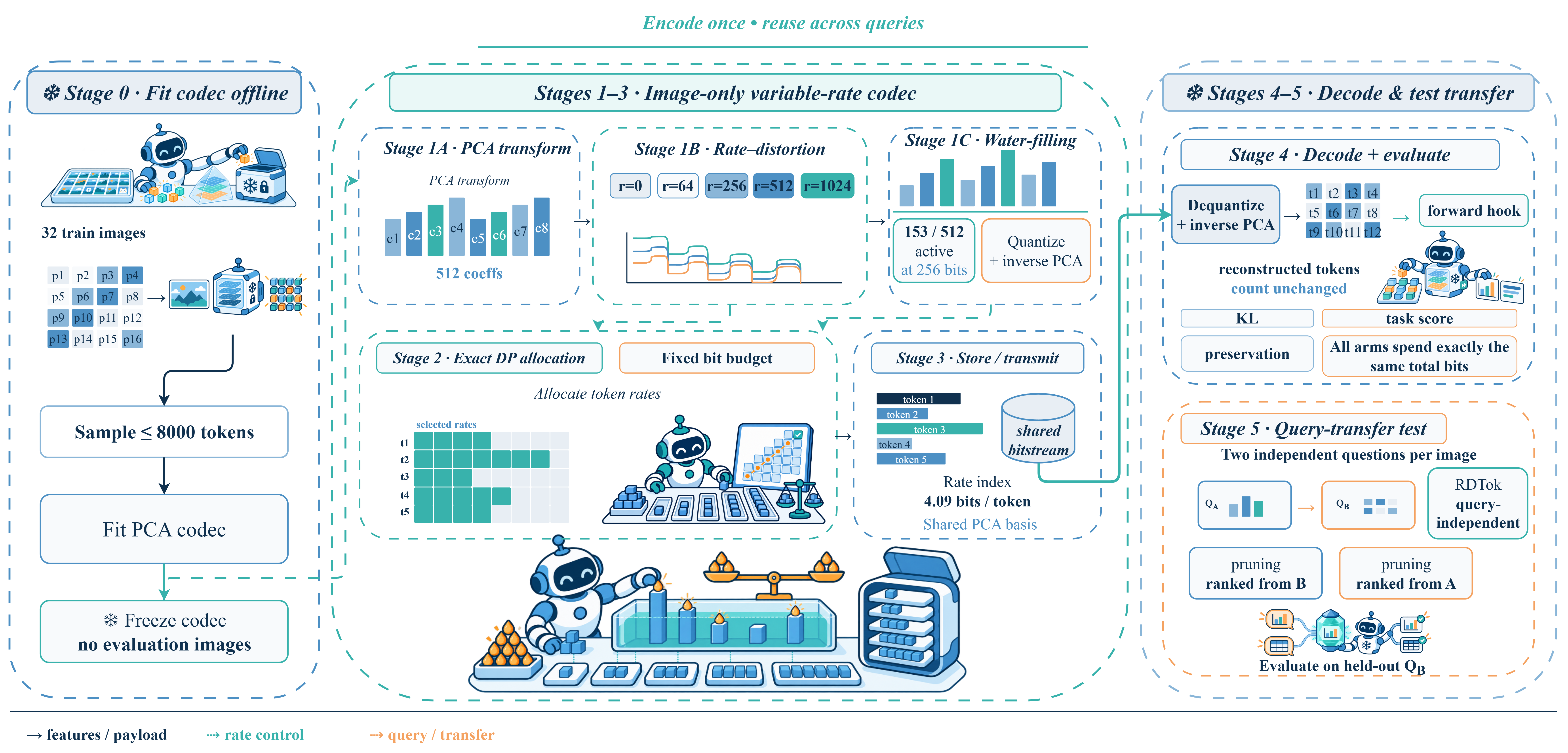
We call the resulting codec RDTok. It has two parts: a transform code that turns each token into a measured distortion–rate curve, and an allocator that spends a fixed bit budget across those curves. Fig. 1 gives the pipeline. Let , , be the visual tokens emitted by the frozen vision tower ( for Qwen3-VL). On tokens from images disjoint from every evaluation image we fit a mean and an orthonormal basis , , and code each token in the coefficient domain, , . By orthonormality the PCA truncation error is independent of the rate, so it is identical for every allocator and cancels in all comparisons below.
Let be the variance of coefficient on the fitting split. Under the high-resolution model , spending bits on a token is minimised by the classical reverse water-fill [10],
| (1) |
with the water level obtained by bisection; the clipped sum is continuous and monotone in , so the budget is met exactly. Each coefficient then receives levels and a uniform mid-tread quantiser over , :
| (2) |
where decodes to the PCA mean. Eq. (1) therefore also selects the active subspace: at bits only of the coefficients are funded, rising to all at .
Rates lie on a uniform grid , , with and bits, so a rate index is interchangeable with a bit count and is the dropped-token analogue. One pass over the grid yields
| (3) |
the measured distortion–rate curve of token . These curves, not a parametric model of them, are what the allocator consumes. A transform code is used rather than a learned vector quantiser because it has an operating range. A shared-codebook residual VQ saturates near nats and is non-monotone in rate, whereas the transform code spans four orders of magnitude and is nearly lossless at full rate (Fig. 2a). The budget, not the codec, then creates the distortion being allocated.
2.2 Allocation across tokens
An allocator is a map with , where are the measured curves and an optional per-token score. Every method compared here is such a map with the same , which makes the comparison equal-rate by construction. Ours uses no :
| (4) |
The objective is separable and the constraint is one scalar resource, so Eq. (4) is solved exactly by dynamic programming over the spent budget [11]. With the least distortion achievable by the first tokens spending exactly steps,
| (5) |
with and otherwise; the optimum is and backtracking the minimising recovers the allocation, ties broken toward the smaller for determinism. Unreachable states are skipped, leaving time; one solve takes ms on average, encoder-side only.
Solving exactly, rather than substituting the closed form of Eq. (1) across tokens, matters for two reasons. The measured obey neither the parametric decay that form assumes nor convexity: only of marginal-gain differences are non-increasing. The closed form is also not scale invariant, so it needs a normalised importance, a knob Eq. (5) does not have.
Baselines as allocators. Uniform rate sets and the closed form substitutes into Eq. (1), both rounded onto with exact sum . Pruning ranks tokens by a score and, with and the induced ordering,
| (6) |
which is exactly the two-valued restriction of Eq. (4)—a feasible but generally suboptimal point of the same programme. It is instantiated with the source score and with the attention score , the mass text positions send to token at a mid-depth layer, which is the token-pruning criterion [1, 2, 3].
Rate accounting and query independence. Each token stores its rate index, bits, of the budget at bits per token; scalar quantisation needs no codebook and amortises over the corpus. Tables report the coefficient budget, identical across arms. No text enters Eqs. (1)–(5): the vision tower does not see the prompt, so and are functions of the image alone. Among the baselines only pruning with the attention score reads the query.
2.3 Why the objective stays on the source side
The evident refinement is to weight Eq. (4) by each region’s measured effect on the output: partition the tokens into contiguous bands, spend one forward pass per band measuring the output KL caused by dropping band , and minimise with , which is Eq. (5) on weighted curves. Such a weighting measures something real—feature MSE is not a sufficient statistic for output KL (Sec. 3.4)—but what it measures is a property of the query it came from, not of the image, and it does not transfer to the next question about the same image. Sec. 3.3 shows the attention score of Eq. (6) has the same defect, which makes this a fact about query-conditioned allocation as a class rather than about one signal.

3 Experiments
Three questions organise the evaluation: whether varying the rate helps at all at a fixed bit budget, whether it helps more than selecting tokens, and what happens when the compressed representation has to serve a question the encoder never saw.
3.1 Protocol
Backbones are the 4B and 8B Qwen3-VL-Instruct models [12], frozen, in float32; datasets are ChartQA [13] (relaxed accuracy) and COCO captions [14], evaluation images per cell, with the basis and quantiser fitted on 32 images from the dataset’s own train split. The three rates, bits per token, are , and compression of the fp16 features; they were chosen per backbone, by the same rule for both, as the band where a measured rate–KL curve is monotone and unsaturated. All arms spend the same total bits. Significance is exact McNemar for the binary metrics and Wilcoxon signed-rank for KL; ∗ marks against RDTok.
| Qwen3-VL-4B | Qwen3-VL-8B | |||||
| Method | KL | Pres. | Acc. | KL | Pres. | Acc. |
| 256 bits/token () | ||||||
| RDTok (ours) | 0.219 | 68.4 | 63.2 | 0.166 | 72.9 | 70.5 |
| Closed-form water-fill | 0.287∗ | 56.2∗ | 54.2∗ | 0.285∗ | 61.1∗ | 63.2∗ |
| Uniform rate | 0.311∗ | 54.9∗ | 52.4∗ | 0.327∗ | 61.5∗ | 60.1∗ |
| Pruning, distortion-rank | 0.510∗ | 46.9∗ | 50.0∗ | 0.432∗ | 50.3∗ | 52.4∗ |
| Pruning, attention-rank | 0.324∗ | 61.1∗ | 63.5 | 0.262 | 68.1 | 70.8 |
| 384 bits/token () | ||||||
| RDTok (ours) | 0.106 | 76.0 | 68.1 | 0.077 | 80.6 | 75.3 |
| Closed-form water-fill | 0.143∗ | 67.4∗ | 62.5∗ | 0.149∗ | 75.7∗ | 71.5∗ |
| Uniform rate | 0.160∗ | 68.1∗ | 60.8∗ | 0.148∗ | 72.9∗ | 70.5∗ |
| Pruning, distortion-rank | 0.392∗ | 59.4∗ | 58.0∗ | 0.239∗ | 70.5∗ | 67.7∗ |
| Pruning, attention-rank | 0.216∗ | 70.1∗ | 68.1 | 0.196∗ | 74.3∗ | 71.2 |
| 512 bits/token () | ||||||
| RDTok (ours) | 0.064 | 80.2 | 69.8 | 0.059 | 85.1 | 76.4 |
| Closed-form water-fill | 0.081∗ | 75.7∗ | 67.7 | 0.072∗ | 81.9 | 74.3 |
| Uniform rate | 0.084∗ | 75.3∗ | 68.8 | 0.082∗ | 81.6 | 76.0 |
| Pruning, distortion-rank | 0.162∗ | 70.5∗ | 66.3 | 0.076∗ | 80.2∗ | 75.7 |
| Pruning, attention-rank | 0.167∗ | 74.7∗ | 69.4 | 0.166∗ | 78.1∗ | 73.6 |
3.2 Main results
Table 1 reports ChartQA at both capacities. Against every query-independent baseline, RDTok lowers output KL in every cell and leads on the other two quantities in all but a couple of COCO cells, and the margins widen as compression becomes more aggressive. That ordering follows from what each arm can express. Uniform rate ignores the heterogeneity of the per-token curves entirely, being the single-level point of Eq. (4), so it overspends on tokens whose distortion has already flattened and underspends on those still descending steeply. Distortion-ranked pruning is the opposite failure. Being the two-valued restriction of the same programme, it commits its whole budget to a quarter of the tokens and discards the rest outright, when a few levels each would have retained most of their content at a fraction of the cost. Both are feasible points of Eq. (4), which is why solving it properly dominates them rather than trading against them.
The closed-form water-fill is the informative negative control, because it also varies the rate and still lands near uniform rate. Fig. 2b explains why: assuming a parametric decay the measured curves do not follow collapses its allocation onto three levels, close to the single level uniform rate uses. The gain therefore comes from taking the distortion–rate curves from measurement, not from varying the rate as such. That is the one design decision the paper most depends on.
The second dataset behaves the same way at both capacities. Across the three rates on COCO captions, RDTok lowers output KL against uniform rate by – at 4B and – at 8B, against the closed-form water-fill by – and –, and against distortion-ranked pruning by – and –. Every comparison reaches , and on 8B RDTok also beats attention-ranked pruning at the most aggressive rate.
Over three seeds at each capacity, each redrawing both splits, RDTok reaches and against and for uniform rate. The ordering is unchanged across those seeds, and across two datasets as different as dense synthetic charts and natural photographs. It does not weaken at the larger capacity either. Against pruning it strengthens, the opposite of the usual pattern for a method developed on a small model.
Attention-ranked pruning is the strongest baseline and the informative comparison. Reading the query, it selects tokens about as well as rate allocation spends bits, matching RDTok on task accuracy, while RDTok, reading only the image, leads it on output KL and on output preservation. Parity with a query-conditioned method at no query cost is already the useful result; it becomes decisive once the compressed representation has to outlive the query. Fig. 3 shows one such case: the pruning arms discard three quarters of the tokens and answer wrongly, while RDTok spreads the same budget over sixteen levels and reproduces the uncompressed answer.
3.3 Query transfer
Every ChartQA test image comes with two independent human questions, so a pruning ranking can be computed from question A and scored on question B, the situation of a cached or transmitted image. Fig. 4 reports it.
Carried to the other question, attention-ranked pruning loses roughly half its fidelity at the smaller capacity and more than doubles its divergence at the larger one, and RDTok leads it at every rate and both capacities. The asymmetry is structural rather than empirical. An attention score marks the regions the current question needs; a distortion–rate curve marks what the image contains. The first is a property of the query and has no reason to survive a change of query; the second is a property of the image and is unchanged by one. A query-independent allocator therefore has no transfer term to lose, which is why its advantage appears here and not in the single-turn comparison above.
The larger model’s attention is the more query-specific, so a larger share of what pruning selects is particular to the question asked, and the value of not conditioning rises with the model. Query-aware selection is thus a trade of reusability for per-query fit, and reusability is precisely what the write-once-read-many setting is made of.
3.4 Analysis
What the allocation looks like. Fig. 2b makes the difference from pruning concrete. RDTok spreads the budget over sixteen levels, pruning has two by construction and uniform rate one. The closed-form water-fill collapses onto three, which is why it tracks uniform rate so closely in Table 1 despite also varying the rate, and why solving on measured curves rather than a parametric model is where the gain comes from.
Why the source objective is not the whole story. Perturbations carrying identical total squared error but different shapes separate the output KL by to at a fixed error level; if feature MSE determined output KL they would coincide. Concentrating the same error on a quarter of the tokens is several times worse than spreading it, and the worst shape is always the high-norm tokens or the leading PCA directions. A source-MSE allocator is therefore optimising a surrogate, which bounds what any allocator working from alone can achieve, and is why the query-weighted variant of Sec. 2.3 was worth trying at all.
References
- [1] L. Chen, H. Zhao, T. Liu, S. Bai, J. Lin, C. Zhou, and B. Chang, “An image is worth 1/2 tokens after layer 2: Plug-and-play inference acceleration for large vision–language models,” in Proc. ECCV, 2024.
- [2] Y. Shang, M. Cai, B. Xu, Y. J. Lee, and Y. Yan, “LLaVA-PruMerge: Adaptive token reduction for efficient large multimodal models,” arXiv:2403.15388, 2024.
- [3] S. Yang, Y. Chen, Z. Tian, C. Wang, J. Li, B. Yu, and J. Jia, “VisionZip: Longer is better but not necessary in vision language models,” in Proc. CVPR, 2025.
- [4] D. Bolya, C.-Y. Fu, X. Dai, P. Zhang, C. Feichtenhofer, and J. Hoffman, “Token merging: Your ViT but faster,” in Proc. ICLR, 2023.
- [5] J. Zou, X. Xu, Z. Wang, Y. Wang, B. Adsumilli, and K. Ma, “RUTA: Principled visual token allocation via rate-utility optimization,” arXiv:2608.04132, 2026.
- [6] J. Zhang, X. Guo, K. Cai, Q. Lv, Y. Fan, W. Chai, J. Wang, and K. Wang, “Hybrid token compression for vision–language models,” in Proc. CVPR, 2026.
- [7] X. Guo and K. Wang, “Adaptive-VoCo: Complexity-aware visual token compression for vision–language models,” arXiv:2512.18496, 2025.
- [8] G. Li, G. Chen, T. Chen, S. Shan, K. Zuo, B. Lyu, T. An, G. Li, and J. Yang, “OccamToken: Efficient VLM inference with training-free and budget-adaptive token pruning,” arXiv:2605.29657, 2026.
- [9] H. Wang, J. Kai, H. Bai, L. Hou, B. Jiang, Z. He, and Z. Lin, “Fourier compressor: Frequency-domain visual token compression for vision–language models,” arXiv:2508.06038, 2025.
- [10] T. M. Cover and J. A. Thomas, Elements of Information Theory, 2nd ed., Wiley, 2006.
- [11] Y. Shoham and A. Gersho, “Efficient bit allocation for an arbitrary set of quantizers,” IEEE Trans. Acoust., Speech, Signal Process., vol. 36, no. 9, pp. 1445–1453, 1988.
- [12] S. Bai et al., “Qwen3-VL technical report,” arXiv:2511.21631, 2025.
- [13] A. Masry, D. X. Long, J. Q. Tan, S. Joty, and E. Hoque, “ChartQA: A benchmark for question answering about charts with visual and logical reasoning,” in Findings of ACL, 2022.
- [14] T.-Y. Lin et al., “Microsoft COCO: Common objects in context,” in Proc. ECCV, 2014.