Data-to-Certificates (D2C): Koopman Supereigenfunctions for Stability, Safety, and Control

Umesh Vaidya IEEE Senior Member ^†^†thanks: Financial support from of NSF CMMI 2031573 is greatly acknowledged. The author is with the Department of Mechanical Engineering, Clemson University, Clemson SC, 29631.

Abstract

Traditional dynamical system models, including Koopman operator representations, are fundamentally equality-based, whereas many analysis and control tools rely on inequalities. This mismatch motivates representations that are intrinsically aligned with certification tasks involved in the analysis and control synthesis problems. In this paper, we propose a data-to-certificates (D2C) paradigm that bypasses explicit model construction and directly learns certificates from data. We introduce supereigenfunctions of the Koopman operator as an inequality-based generalization of eigenfunctions that define exponential growth envelopes encoding stability, safety, and uncertainty propagation, thereby serving as certificates for a range of control objectives. We establish their theoretical foundations and show that the associated rates recover intrinsic dynamical quantities such as Lyapunov exponents. Two complementary constructions are developed: a geometric approach based on the multiplicative ergodic theorem (MET), and a resolvent/Gramian formulation that enables computation directly from trajectory data. The resulting framework yields certificates that can be used for stability and contraction analysis, as well as stabilizing and safety-critical control synthesis via convex quadratic programming-based optimization program. Numerical examples demonstrate the effectiveness of the proposed data-driven certification approach for stabilization, contraction, and safe control design.

I Introduction

Models of dynamical systems are not ends in themselves but they are instruments for prediction, analysis, and control synthesis. From this perspective, the structure of a model should be dictated by the tasks it is meant to enable. Classical modeling paradigms including linear system representations and operator-theoretic approaches such as Koopman operator theory are predominantly equality-based, describing system evolution through exact relations. In contrast, most of the powerful tools in systems and control, including Lyapunov stability theory, Hamilton–Jacobi (HJ) formulations for optimal control, and safety verification via barrier functions, are fundamentally inequality-based. This reveals a structural mismatch between how models are constructed and how they are ultimately used.

Koopman operator theory provides a compelling framework for the analysis and control of nonlinear dynamical systems by lifting them into a linear space of observables [1, 2, 3, 4, 5, 6, 7, 8, 9, 10, 11]. In this setting, Koopman eigenfunctions define intrinsic coordinates in which the dynamics evolve linearly, enabling prediction and control. However, this framework is built on spectral equalities of the form $\mathcal{K}_{f}\phi=\lambda\phi$ , which encode exact exponential evolution. While elegant, this representation faces well-known limitations: global eigenfunctions may fail to exist, the spectrum may be continuous or ill-defined, and for controlled systems the lifted dynamics become bilinear, complicating synthesis [3, 9, 12].

In contrast, synthesis methodologies such as Lyapunov theory, control Lyapunov and barrier functions, and HJ-based approaches are inherently inequality-driven. These methods characterize system behavior through bounds, envelopes, and certificates rather than exact representations. For example, Lyapunov functions certify stability via $\dot{V}\leq-\alpha(V)$ , while HJ value functions encode optimality through viscosity inequalities [13, 14, 15]. These approaches emphasize certification rather than representation.

This paper proposes a unifying perspective that bridges these two paradigms. We introduce supereigenfunctions of the Koopman operator, defined by relaxing the spectral equality to a one-sided inequality

\mathcal{K}_{f}\phi\leq\lambda\phi.

This seemingly simple relaxation fundamentally changes the role of the representation. Instead of encoding exact trajectory evolution, supereigenfunctions define exponential growth envelopes that bound system behavior. As a result, they provide an operator-theoretic representation that is naturally compatible with Lyapunov functions, HJ value functions, and reachability and safety certificates [16, 17, 18, 19, 20].

The key conceptual shift of this work is that Koopman-based methods are no longer used to construct predictive models, but to construct certificates. In this view, supereigenfunctions act as operator-theoretic analogues of Lyapunov and value functions, enabling stability, safety, and performance guarantees directly within the Koopman framework.

We develop the theory of supereigenfunctions along two complementary directions. First, we introduce directional supereigenfunctions, defined on the tangent bundle, which capture anisotropic growth and contraction rates. These objects arise naturally from the multiplicative ergodic theorem (MET), with associated rates corresponding to Lyapunov exponents, thereby providing a geometric and dynamical interpretation of the framework [21, 22]. Second, we develop a resolvent-based construction that generates families of supereigenfunctions from user-defined probe functions. This construction admits trajectory-based representations and enables computation directly from data, without explicit knowledge of the system.

A key feature of the proposed framework is that supereigenfunctions are globally defined, nonnegative, and form a convex cone. Moreover, their inherent non-uniqueness becomes a design degree of freedom: different choices correspond to different objectives, such as stabilization, safety, or uncertainty quantification. This enables a task-driven representation paradigm in which the choice of observables is aligned with the intended analysis or control objective. This is in contrast to the choice of observables or lifting function used for the finite dimensional approximation of the Koopman opertor or its spectrum where the focus in on discovering intrinsic coordinates or subspace for minimal linear representation of nonlinear system.

Importantly, the proposed constructions admit data-driven implementations. In particular, resolvent-based approach allow supereigenfunctions to be computed directly from trajectory data and variational dynamics. This provides a scalable alternative to PDE-based or sum-of-squares [23, 24, 25, 26, 27] approaches and enables integration with modern learning-based pipelines, including high-fidelity simulators and world models [28, 29, 30]. As a result, the framework supports the direct extraction of provable guarantees from data.

It is important to distinguish the proposed supereigenfunction framework from classical control Lyapunov and barrier functions (CLFs/CBFs) as well as standard Koopman eigenfunctions. CLFs and CBFs are inequality-based certificates typically constructed heuristically or via optimization (e.g., sum-of-squares), and are often problem-specific. In contrast, supereigenfunctions arise directly from the Koopman operator, providing certificates that reflect the intrinsic system dynamics and can be computed from trajectory data. While the construction differs fundamentally, the resulting control synthesis has a similar structure: both approaches lead to pointwise convex QPs enforcing inequality constraints. However, in the proposed framework, these constraints are derived from operator-theoretic constructions rather than imposed on candidate functions, yielding a data-driven and dynamically consistent alternative to classical certificate design.

The contributions of this paper are as follows. We introduce supereigenfunctions as an inequality-based generalization of Koopman eigenfunctions and establish their role as operator-theoretic certificates for nonlinear dynamical systems. We develop directional supereigenfunctions on the tangent bundle and show that they recover and generalize contraction-based stability and incremental analysis. We propose resolvent and trajectory-based constructions that enable computation of supereigenfunctions directly from data. We establish connections between the proposed framework and Lyapunov theory, contraction theory, and safety certification, providing a unified operator-theoretic perspective. We show that supereigenfunction-based certificates lead to convex control synthesis via quadratic programs (QPs), unifying stabilization, safety, and contraction within a single optimization framework. We demonstrate the effectiveness of the approach through applications to uncertainty propagation, stabilizing control, safety filtering, and synchronization. Overall, this work establishes a new paradigm in which Koopman theory is used not for modeling system trajectories, but for constructing certificates that enable analysis and control of nonlinear systems.

II Preliminaries and Notations

II-A Notations

Let $\Omega\subset\mathbb{R}^{n}$ denote the state space and $s_{t}:\Omega\to\Omega$ the flow generated by the dynamical system $\dot{x}=f(x).$ For vectors $x,y\in\mathbb{R}^{m}$ , the notation $x\preceq y$ denotes componentwise ordering, $x_{i}\leq y_{i},\;i=1,\ldots,m.$ For symmetric matrices $A,B\in\mathbb{S}^{n}$ , $A\preceq B$ denotes the Loewner partial order, $B-A\succeq 0.$ The usual scalar ordering is denoted by $\leq$ . The cone of nonnegative vectors is denoted by $\mathbb{R}^{m}_{+}:=\{x\in\mathbb{R}^{m}:\ x_{i}\geq 0,\ i=1,\ldots,m\}.$ The sets of symmetric positive semidefinite and positive definite matrices are denoted by $\mathbb{S}_{+}^{n}$ and $\mathbb{S}_{++}^{n},$ respectively.

II-B Koopman Operator

This section reviews the Koopman operator framework for nonlinear autonomous dynamical systems and recalls Koopman eigenfunctions. Let $\Omega\subseteq\mathbb{R}^{n}$ be an open set and consider the system

\dot{x}=f(x),\qquad f\in C^{1}(\Omega,\mathbb{R}^{n}).

(1)

We assume forward completeness, i.e., for every $x\in\Omega$ the solution exists for all $t\geq 0$ and remains in $\Omega$ . Let $s_{t}:\Omega\to\Omega$ denote the associated flow. Koopman theory studies the evolution of observables $\phi:\Omega\to\mathbb{R}$ rather than states [31]. Let $\mathcal{F}$ be a function space such as $C^{1}(\Omega)$ or $L^{2}(\Omega,\mu)$ . The Koopman operator $U_{t}:\mathcal{F}\to\mathcal{F}$ is defined

(U_{t}\phi)(x):=\phi(s_{t}(x)).

(2)

The family $\{U_{t}\}_{t\geq 0}$ forms a strongly continuous semigroup with $U_{t+\tau}=U_{t}U_{\tau}$ and $U_{0}=I$ . Each $U_{t}$ is linear even when (1) is nonlinear. The infinitesimal generator of $\{U_{t}\}$ is

\mathcal{K}_{f}\phi:=\lim_{t\downarrow 0}\frac{U_{t}\phi-\phi}{t},

(3)

whenever the limit exists. For $\phi\in C^{1}(\Omega)$ ,

(\mathcal{K}_{f}\phi)(x):=\nabla\phi(x)\cdot f(x),

(4)

i.e., $\mathcal{K}_{f}$ coincides with differentiation along trajectories.

Definition 1 (Koopman eigenfunction)

A nonzero observable $\phi\in\mathcal{F}$ is a Koopman eigenfunction with eigenvalue $\lambda\in\mathbb{C}$ if

\mathcal{K}_{f}\phi=\lambda\phi.

(5)

Equivalently,

\phi(s_{t}(x))=e^{\lambda t}\phi(x),\qquad\forall t\geq 0.

(6)

If $\{\phi_{i}\}_{i=1}^{m}$ are eigenfunctions with eigenvalues $\lambda_{i}$ , then the lifted coordinates $z_{i}=\phi_{i}(x)$ satisfy $\dot{z}_{i}=\lambda_{i}z_{i}$ , yielding linear, decoupled dynamics. For linear systems $\dot{x}=Ax$ , if $w^{\top}A=\lambda w^{\top}$ , then $\phi(x)=w^{\top}x$ is a Koopman eigenfunction with eigenvalue $\lambda$ . For general nonlinear systems, smooth global eigenfunctions may fail to exist or may only be defined locally [3]—for example, in the presence of multiple attractors or complex recurrent dynamics. Moreover, systems with continuous or ill-conditioned Koopman spectra pose significant challenges for spectral approximation. .The equality (5) can be fragile under perturbations and difficult to enforce from data. These limitations motivate inequality-based objects that preserve growth information while relaxing spectral equality.

III Supereigenfunctions of the Koopman Operator

From the perspective of positive operator theory, the Koopman semigroup preserves pointwise order, and supereigenfunctions arise naturally as cone-ordered subeigenfunctions of positive operator [32, 33].

III-A Ordered spaces and positivity

Let $\mathcal{F}$ be a real Banach space of observables on $\Omega$ (e.g., $C(\Omega)$ , $C^{1}(\Omega)$ , or $L^{p}(\Omega,\mu)$ ), equipped with the positive cone

\mathcal{F}_{+}:=\{\psi\in\mathcal{F}:\psi(x)\geq 0\ \text{(a.e.) in }\Omega\}.

This cone induces the partial order $\psi_{1}\leq\psi_{2}$ iff $\psi_{1}-\psi_{2}\in\mathcal{F}_{+}$ . An operator $T:\mathcal{F}\to\mathcal{F}$ is positive if $\phi\in\mathcal{F}_{+}$ implies $T\phi\in\mathcal{F}_{+}$ . The Koopman semigroup $(U_{t})_{t\geq 0}$ forms a positive semigroup on $\mathcal{F}$ , preserving the cone $\mathcal{F}_{+}$ [34, 31]. Indeed as $U_{t}:\mathcal{F}\to\mathcal{F}$ defined by $(U_{t}\psi)(x):=\psi(s_{t}(x))$ positivity follows:

\psi\in\mathcal{F}_{+}\ \Longrightarrow\ U_{t}\psi\in\mathcal{F}_{+},\qquad\forall t\geq 0.

(7)

In this ordered setting, one may study subeigenfunctions (also called cone subeigenvectors).

III-B Supereigenfunctions and envelope rates

Definition 2 (Supereigenfunction)

A function $\varphi:\Omega\to\mathbb{R}_{\geq 0}$ is a supereigenfunction of $\mathcal{K}_{f}$ if there exists $\lambda\in\mathbb{R}$ such that

(\mathcal{K}_{f}\varphi)(x)\leq\lambda\varphi(x),\qquad\forall x\in\Omega.

(8)

Any such $\lambda$ is called an admissible supereigenvalue.

Along the trajectories of the system $s_{t}(x)$ , we have

\frac{d}{dt}\varphi(x(t))\leq\lambda\varphi(x(t)),

so $\varphi$ is bounded by an exponential envelope. Unlike eigenfunctions, which may be complex-valued and sign-changing, supereigenfunctions are nonnegative and encode growth bounds. The focus of this paper is on the supereigenfunctions of the Koopman operator as defined above, however we define the subeigenfunctions as below for completeness.

Definition 3 (Subeigenfunction)

A nonnegative observable $\varphi:\Omega\to\mathbb{R}_{\geq 0}$ is called a subeigenfunction of $\mathcal{K}_{f}$ with rate $\lambda\in\mathbb{R}$ if

\mathcal{K}_{f}\varphi\geq\lambda\varphi.

Proposition 1 (Exponential envelope)

If $\varphi$ satisfies (8), then

\varphi(s_{t}(x))\leq e^{\lambda t}\varphi(x),\qquad\forall t\geq 0,\ \forall x\in\Omega,

(9)

equivalently $U_{t}\varphi\leq e^{\lambda t}\varphi$ .

Proof:

Apply Grönwall’s inequality.∎∎

The following connects equality-based and inequality-based representations.

Proposition 2 (From eigenfunctions to envelopes)

If $\phi$ satisfies $\mathcal{K}_{f}\phi=\lambda\phi$ for some $\lambda\in\mathbb{C}$ , then $\psi:=|\phi|^{2}$ satisfies

\mathcal{K}_{f}\psi=2\,\mathrm{Re}(\lambda)\,\psi.

Thus $\psi$ is both a supereigenfunction and a subeigenfunction with rate $2\,\mathrm{Re}(\lambda)$ .

Proof:

Since $\psi=|\phi|^{2}=\phi\,\overline{\phi},$ the product rule for the Koopman generator gives

\mathcal{K}_{f}\psi=(\mathcal{K}_{f}\phi)\,\overline{\phi}+\phi\,\mathcal{K}_{f}\overline{\phi}.

Because the vector field $f$ is real-valued, $\mathcal{K}_{f}\overline{\phi}=\overline{\mathcal{K}_{f}\phi}.$ Using the eigenfunction relation $\mathcal{K}_{f}\phi=\lambda\phi,$ we therefore obtain

	$\displaystyle\mathcal{K}_{f}\|\phi\|^{2}$	$\displaystyle=\lambda\phi\overline{\phi}+\phi\,\overline{\lambda\phi}=\lambda\|\phi\|^{2}+\overline{\lambda}\|\phi\|^{2}$
		$\displaystyle=(\lambda+\overline{\lambda})\|\phi\|^{2}=2\,\mathrm{Re}(\lambda)\|\phi\|^{2}.$

Hence, with $\psi=|\phi|^{2}$ ,

\mathcal{K}_{f}\psi=2\,\mathrm{Re}(\lambda)\psi.

Since $\psi\geq 0$ , equality implies both

\mathcal{K}_{f}\psi\leq 2\,\mathrm{Re}(\lambda)\psi\;\;{\rm and}\;\;\mathcal{K}_{f}\psi\geq 2\,\mathrm{Re}(\lambda)\psi.

Thus $\psi$ is simultaneously a supereigenfunction and a subeigenfunction with rate $2\,\mathrm{Re}(\lambda)$ . ∎

III-C Minimal rates and Collatz–Wielandt interpretation

Supereigenvalues are not unique: if (8) holds for $\lambda$ , it holds for any $\lambda^{\prime}\geq\lambda$ . This motivates an intrinsic rate.

Definition 4 (Minimal supereigenvalue)

For $\varphi\geq 0$ , define

\lambda_{\varphi}:=\inf\{\lambda\in\mathbb{R}:\mathcal{K}_{f}\varphi\leq\lambda\varphi\}.

(10)

If $\varphi\in C^{1}(\Omega)$ and $\varphi(x)>0$ , then

\lambda_{\varphi}=\sup_{x\in\Omega}\frac{(\mathcal{K}_{f}\varphi)(x)}{\varphi(x)}.

(11)

This is a continuous-time analogue of the Collatz–Wielandt bound from Perron–Frobenius theory [35, 36], extended to positive operators and their generators [33, 37, 34]. It provides the tightest exponential envelope certified by $\varphi$ .

III-D Cone properties and existence

Supereigenfunctions form a convex cone i.e., Scaling: $c\varphi$ is a supereigenfunction for $c>0$ , Addition: $\varphi_{1}+\varphi_{2}$ has rate $\max\{\lambda_{1},\lambda_{2}\}$ . They also exist under mild conditions.

Theorem 1 (Global supereigenfunction)

Suppose

\|f(x)\|\leq L(1+\|x\|),\qquad x\in\Omega.

Then

\varphi(x)=1+\|x\|^{2}

is a global supereigenfunction satisfying

\mathcal{K}_{f}\varphi(x)\leq 3L\,\varphi(x),\qquad x\in\Omega.

Proof:

Since $\nabla\varphi(x)=2x$ ,

\mathcal{K}_{f}\varphi(x)=2x^{\top}f(x)\leq 2\|x\|\,\|f(x)\|\leq 2L\|x\|(1+\|x\|).

Using $2\|x\|\leq 1+\|x\|^{2}$ ,

	$\displaystyle\mathcal{K}_{f}\varphi(x)$	$\displaystyle\leq 2L\\|x\\|+2L\\|x\\|^{2}$
		$\displaystyle\leq L(1+\\|x\\|^{2})+2L\\|x\\|^{2}$
		$\displaystyle\leq 3L(1+\\|x\\|^{2})=3L\varphi(x).$

∎

III-E Examples: eigenfunctions versus supereigenfunctions

The following examples highlight the distinction between Koopman eigenfunctions, which encode exact spectral evolution, and supereigenfunctions, which provide nonnegative growth envelopes.

III-E1 Linear systems

Consider the linear system $\dot{x}=Ax$ on $\mathbb{R}^{n}$ . If $w_{i}^{\top}A=\mu_{i}w_{i}^{\top}$ , then $\phi_{i}(x)=w_{i}^{\top}x$ is a Koopman eigenfunction satisfying $\mathcal{K}_{f}\phi_{i}=\mu_{i}\phi_{i}$ . These eigenfunctions may be complex-valued. A nonnegative quadratic observable

\psi_{i}(x):=|\phi_{i}(x)|^{2},

gives $\mathcal{K}_{f}\psi_{i}=2\,\mathrm{Re}(\mu_{i})\,\psi_{i},\;\;\psi_{i}(s_{t}(x))=e^{2\mathrm{Re}(\mu_{i})t}\psi_{i}(x).$ Thus $\psi_{i}$ is a supereigenfunction with rate $2\,\mathrm{Re}(\mu_{i})$ . This shows that in the linear setting supereigenfunctions recover the quadratic growth envelopes associated with spectral modes.

III-E2 Triangular nonlinear system: resonance and loss of smooth eigenfunctions

Consider

\dot{x}_{1}=\mu x_{1},\qquad\dot{x}_{2}=\beta x_{2}+x_{1}^{2},\qquad(\mu,\beta\in\mathbb{R}).

(12)

The observable $\phi_{1}(x)=x_{1}$ is always a Koopman eigenfunction with eigenvalue $\mu$ . To construct an eigenfunction associated with $\beta$ , use the ansatz

\phi_{2}(x)=x_{2}+h(x_{1}),

which leads to $\mu x_{1}h^{\prime}(x_{1})-\beta h(x_{1})+x_{1}^{2}=0.$ If $\beta\neq 2\mu$ , this admits the smooth solution

\phi_{2}(x)=x_{2}-\frac{x_{1}^{2}}{2\mu-\beta},

so $\phi_{2}$ is a Koopman eigenfunction with eigenvalue $\beta$ . In the resonant case $\beta=2\mu$ , however, the solution involves logarithmic terms and is not smooth at the origin; hence no smooth eigenfunction of this form exists. Despite this failure of spectral equality, one can still construct a global supereigenfunction. For example, for any $k>0$ ,

\varphi(x):=x_{1}^{2}+x_{2}^{2}+kx_{1}^{4}

(13)

satisfies $\mathcal{K}_{f}\varphi\leq\lambda\varphi$ where $\lambda=\max\left\{0,2\mu,\;4\mu+\frac{1}{\sqrt{k}}\right\}$ . Thus even when smooth eigenfunctions break down under resonance, a supereigenfunction remains.

III-E3 Local eigenfunctions versus global supereigenfunctions

Consider the scalar nonlinear system

\dot{x}=-x+x^{3}=-x(1-x^{2}),\qquad x\in\mathbb{R}.

(14)

The origin is locally asymptotically stable with domain of attraction $|x|<1$ , while $x=\pm 1$ are unstable equilibria. For this system, one obtains the Koopman eigenfunction

\phi(x)=\frac{x}{\sqrt{1-x^{2}}},

(15)

which satisfies $\mathcal{K}_{f}\phi=-\phi.$ However, $\phi$ is well defined only for $|x|<1$ and diverges as $x\to\pm 1$ . Thus, the eigenfunction is confined to the basin of attraction of the origin and cannot be extended globally. In contrast, consider the globally defined nonnegative observable

\varphi(x)=e^{-x^{2}}.

A direct computation gives

\mathcal{K}_{f}\varphi=\nabla\varphi(x)f(x)=(-2xe^{-x^{2}})(-x+x^{3})=(2x^{2}-2x^{4})\varphi(x).

Since $\sup_{x\in\mathbb{R}}(2x^{2}-2x^{4})=\tfrac{1}{2},$ it follows that

\mathcal{K}_{f}\varphi\leq\tfrac{1}{2}\,\varphi(x),

so $\varphi$ is a global supereigenfunction with rate $\lambda=\tfrac{1}{2}$ . This example illustrates a key advantage of the inequality-based formulation: Koopman eigenfunctions may be only locally defined, whereas supereigenfunctions can be constructed globally, valid beyond the basin of attraction.

III-E4 Mechanical energy as a global supereigenfunction

Consider a mechanical system with generalized coordinates $q\in\mathbb{R}^{n}$ and velocities $v=\dot{q}\in\mathbb{R}^{n}$ , governed by

M(q)\dot{v}+C(q,v)v+\nabla V(q)+D(q,v)v=0,

(16)

together with $\dot{q}=v$ . Here $M(q)\in\mathbb{S}_{++}^{n}$ is the inertia matrix, $V(q)$ is the potential energy, and $D(q,v)\in\mathbb{S}_{+}^{n}$ is a damping matrix. Assume the standard identity $\dot{M}(q)-2C(q,v)\ \text{is skew-symmetric}.$ Define the total energy

E(q,v)=\frac{1}{2}v^{\top}M(q)v+V(q).

(17)

Then,

\frac{d}{dt}E(q(t),v(t))=-\,v(t)^{\top}D(q(t),v(t))v(t)\leq 0,

(18)

and therefore

\mathcal{K}_{f}E(x)\leq 0.

(19)

Hence $E$ is a global supereigenfunction with admissible rate $\lambda=0$ . This example is representative of the certificate viewpoint developed in the paper: the total energy is not generally a Koopman eigenfunction, but it is a physically meaningful, globally defined inequality certificate directly aligned with stability and control analysis.

IV Directional Supereigenfunctions

Scalar supereigenfunctions provide global envelopes of the form $\mathcal{K}_{f}\varphi\leq\lambda\varphi,$ but a single rate may be conservative when the dynamics exhibit anisotropic growth or contraction. This motivates directional supereigenfunctions, i.e., families

\mathcal{K}_{f}\varphi_{i}\leq\lambda_{i}\varphi_{i},\qquad i=1,\dots,m,

with each component capturing a distinct direction and rate. We present two complementary constructions: a geometric one based on tangent dynamics and the multiplicative ergodic theorem (MET), and one based on resolvent equations.

IV-A Directional envelopes from tangent dynamics

Directional supereigenfunctions arise naturally from tangent dynamics, where anisotropic growth of perturbations induces multiple rates. We formalize this through metric-based constructions and their connection to the MET.

IV-A1 Tangent dynamics and metric characterization

Let $f\in C^{1}(\Omega,\mathbb{R}^{n})$ generate the flow $s_{t}$ . The variational system

\dot{v}=Df(x(t))\,v,\qquad v(t)=Y(t,x)v(0),

(20)

defines the tangent cocycle $Y(t,x):=Ds_{t}(x)$ . For observables $\varphi:\Omega\times\mathbb{R}^{n}\to\mathbb{R}$ defined on the tangent bundle, the extended dynamics

\displaystyle\dot{x}=f(x),\qquad\dot{v}=Df(x)v

(21)

induces the tangent-space Koopman operator and generator

	$\displaystyle(U^{\tan}_{t}\varphi)(x,v)$	$\displaystyle:=\varphi(s_{t}(x),Y(t,x)v)$
	$\displaystyle(\mathcal{K}_{f}^{\tan}\varphi)(x,v)$	$\displaystyle:=\nabla_{x}\varphi(x,v)^{\top}f(x)+\nabla_{v}\varphi(x,v)^{\top}Df(x)v.$		(22)

Proposition 3 (Metric characterization)

Let $\varphi_{M}(x,v):=v^{\top}M(x)v,\;\;M:\Omega\to\mathbb{S}_{+}^{n}.$ Then

(\mathcal{K}_{f}^{\tan}\varphi_{M})(x,v)\leq\lambda\,\varphi_{M}(x,v)\qquad\forall(x,v)\in\Omega\times\mathbb{R}^{n}

if and only if

Df(x)^{\top}M(x)+M(x)Df(x)+\dot{M}(x)\preceq\lambda\,M(x),\;\;\forall x\in\Omega,

\dot{M}(x):=(\nabla M(x))\cdot f(x)=\sum_{k=1}^{n}\frac{\partial M(x)}{\partial x_{k}}f_{k}(x).

Proof:

The result follows by differentiating

\varphi_{M}(x,v)=v^{\top}M(x)v

along the tangent dynamics (21) which gives

(\mathcal{K}_{f}^{\tan}\varphi_{M})(x,v)=v^{\top}\big(Df^{\top}M+MDf+\dot{M}\big)v.

The inequality then holds for all $v$ if and only if the stated matrix inequality is satisfied.∎∎Thus, directional supereigenfunctions correspond to matrix differential inequalities, closely related to contraction metrics.

IV-A2 Asymptotic construction via MET

Assume $\mu$ is invariant and $\log^{+}\|Df\|\in L^{1}(\mu)$ . By the MET, for $\mu$ -a.e. $x$ there exist Lyapunov exponents $\chi_{1}>\cdots>\chi_{r}$ and an Oseledets splitting

T_{x}\Omega=E_{1}(x)\oplus\cdots\oplus E_{r}(x),\;\;\lim_{t\to\infty}\frac{1}{t}\log\|Y(t,x)v\|=\chi_{i}.

for $v\in E_{i}(x)\setminus\{0\}$ . Let $P_{i}(x)$ denote the orthogonal projector onto $E_{i}(x)$ and define

\varphi_{i}(x,v):=\|P_{i}(x)v\|^{2}.

(23)

Theorem 2 (Directional supereigenfunctions from MET)

For $\mu$ -a.e. $x$ and $P_{i}(x)v\neq 0$ , for $\varphi_{i}(x,v)$ as defined in (23), we have

\lim_{t\to\infty}\frac{1}{t}\log\varphi_{i}(s_{t}(x),Y(t,x)v)=2\chi_{i}.

Equivalently, for any $\varepsilon>0$ ,

\varphi_{i}(s_{t}(x),Y(t,x)v)\leq e^{(2\chi_{i}+\varepsilon)t}\varphi_{i}(x,v)\quad\text{for large }t.

Proof:

By the multiplicative ergodic theorem (MET) [21], for $\mu$ -a.e. $x$ there exists an invariant splitting

T_{x}\Omega=E_{1}(x)\oplus\cdots\oplus E_{r}(x),\;\;Y(t,x)E_{j}(x)=E_{j}(s_{t}(x)),

with associated Lyapunov exponents $\chi_{j}$ . Let $P_{i}(x)$ denote the projector onto $E_{i}(x)$ . Then

P_{i}(s_{t}(x))\,Y(t,x)=Y(t,x)\,P_{i}(x).

Hence, for any $v$ such that $P_{i}(x)v\neq 0$ ,

		$\displaystyle\varphi_{i}\bigl(s_{t}(x),Y(t,x)v\bigr)=\bigl\\|P_{i}(s_{t}(x))Y(t,x)v\bigr\\|^{2}$
		$\displaystyle=\bigl\\|Y(t,x)P_{i}(x)v\bigr\\|^{2}.$		(24)

Since $P_{i}(x)v\in E_{i}(x)\setminus\{0\}$ , the MET gives

\lim_{t\to\infty}\frac{1}{t}\log\bigl\|Y(t,x)P_{i}(x)v\bigr\|=\chi_{i}.

Therefore,

\lim_{t\to\infty}\frac{1}{t}\log\varphi_{i}\bigl(s_{t}(x),Y(t,x)v\bigr)=2\chi_{i}.

Consequently, for any $\varepsilon>0$ , there exists $T=T(x,v,\varepsilon)>0$ such that for all $t\geq T$ ,

(U^{\tan}_{t}\varphi_{i})(x,v)\leq e^{(2\chi_{i}+\varepsilon)t}\varphi_{i}(x,v).

Thus, $\varphi_{i}$ defines an asymptotic directional supereigenfunction with rate $2\chi_{i}$ along typical trajectories.∎∎

IV-A3 Adapted metrics from Oseledets directions

For weights $w_{i}>0$ , define

M(x):=\sum_{i=1}^{r}w_{i}P_{i}(x),\;\;\varphi_{M}(x,v)=\sum_{i=1}^{r}w_{i}\|P_{i}(x)v\|^{2}.

(25)

Proposition 4 (Adapted metric supereigenfunction)

$\varphi_{M}$ is an asymptotic supereigenfunction with rate $2\chi_{\max}$ , where $\chi_{\max}=\max\{\chi_{i}:\ w_{i}>0\}$ .

This provides a systematic construction of contraction-type metrics from the MET decomposition.

IV-A4 Infinite-horizon Gramian construction

A constructive realization of directional supereigenfunctions can be obtained directly from tangent dynamics via an infinite-horizon Gramian.

Let $Q:\Omega\to\mathbb{S}_{+}^{n}$ and $\lambda>0$ . Define

M_{\lambda}(x):=\int_{0}^{\infty}e^{-2\lambda t}\,Y(t,x)^{\top}Q\big(s_{t}(x)\big)\,Y(t,x)\,dt,

(26)

whenever the integral converges. The associated observable is

\varphi_{\lambda}(x,v)=v^{\top}M_{\lambda}(x)v=\int_{0}^{\infty}e^{-2\lambda t}\|Q^{1/2}(s_{t}(x))Y(t,x)v\|^{2}dt.

(27)

Proposition 5 (Family of Gramian-based directional supereigenfunctions)

Let $Q_{i}:\Omega\to\mathbb{S}_{+}^{n}$ and $\lambda_{i}>0$ , $i=1,\dots,m$ , and define

M_{i}(x):=\int_{0}^{\infty}e^{-2\lambda_{i}t}\,Y(t,x)^{\top}Q_{i}\big(s_{t}(x)\big)\,Y(t,x)\,dt,

(28)

whenever the integral converges. For each $i$ , define

\varphi_{i}(x,v):=v^{\top}M_{i}(x)v=\int_{0}^{\infty}e^{-2\lambda_{i}t}\|Q_{i}^{1/2}(s_{t}(x))\,Y(t,x)v\|^{2}\,dt.

(29)

Then each $\varphi_{i}$ satisfies

(\mathcal{K}_{f}^{\mathrm{tan}}\varphi_{i})(x,v)=2\lambda_{i}\,\varphi_{i}(x,v)-v^{\top}Q_{i}(x)v,

(30)

and hence

(\mathcal{K}^{\mathrm{tan}}_{f}\varphi_{i})(x,v)\leq 2\lambda_{i}\,\varphi_{i}(x,v).

(31)

Therefore, $\{\varphi_{i}\}_{i=1}^{m}$ defines a family of directional supereigenfunctions on the tangent bundle.

Remark 3 (Relation to Lyapunov exponents)

The convergence of (26) requires the discount rate $\lambda$ to dominate the asymptotic growth of the tangent dynamics. In particular, if $\chi_{\max}$ denotes the largest Lyapunov exponent in the directions weighted by $Q$ , then a sufficient condition for convergence is $\lambda>\chi_{\max}$ . Thus, $\lambda$ acts as a design upper bound on directional growth rates, linking the Gramian construction to the MET-based characterization.

IV-B Data-to-Certificate Construction via Positive Resolvents

We next develop a trajectory-based construction of Koopman supereigenfunctions using the resolvent of the Koopman generator. The central idea is to select a nonnegative probe function that encodes the quantity of interest and map it directly to a certificate through the positive resolvent. This provides a data-to-certificate (D2C) construction: the certificate can be evaluated from trajectory rollouts without first identifying an intermediate dynamical model or a finite-dimensional Koopman representation.

Let $\{U_{t}\}_{t\geq 0}$ denote the positive Koopman $C_{0}$ -semigroup on the Banach lattice $\mathcal{F}$ , with infinitesimal generator $\mathcal{K}_{f}$ . Assume that the semigroup is exponentially bounded,

\|U_{t}\|\leq Me^{\omega t},\qquad t\geq 0,

(32)

for some $M\geq 1$ and $\omega\in\mathbb{R}$ . For $\lambda>\omega$ , the resolvent of $\mathcal{K}_{f}$ is

R(\lambda;\mathcal{K}_{f}):=(\lambda I-\mathcal{K}_{f})^{-1}=\int_{0}^{\infty}e^{-\lambda t}U_{t}\,dt.

(33)

Since $U_{t}$ is positive, $R(\lambda;\mathcal{K}_{f})$ is also a positive operator. Thus, a nonnegative probe $g\in\mathcal{F}_{+}$ is mapped to a nonnegative observable

\varphi_{\lambda}=R(\lambda;\mathcal{K}_{f})g=\int_{0}^{\infty}e^{-\lambda t}U_{t}g\,dt=\int_{0}^{\infty}e^{-\lambda t}g(s_{t}(x))\,dt.

(34)

The following theorem summarizes the resulting exact, finite-rollout, and approximate certificate properties.

Theorem 4 (Positive-resolvent data-to-certificate theorem)

Let $\{U_{t}\}_{t\geq 0}$ be a positive Koopman $C_{0}$ -semigroup on $\mathcal{F}$ satisfying (32), and let $g\in\mathcal{F}_{+}$ . For $\lambda>\omega$ , define

\varphi_{\lambda}:=R(\lambda;\mathcal{K}_{f})g.

(35)

Then the following statements hold.

(i)

Exact positive certificate. The function $\varphi_{\lambda}\in D(\mathcal{K}_{f})$ is nonnegative and satisfies

$(\lambda I-\mathcal{K}_{f})\varphi_{\lambda}=g.$ (36)

Consequently,

$\mathcal{K}_{f}\varphi_{\lambda}=\lambda\varphi_{\lambda}-g\leq\lambda\varphi_{\lambda},$ (37)

and hence $\varphi_{\lambda}$ is a Koopman supereigenfunction with rate $\lambda$ .

(ii)

Finite-rollout certificate. For $T>0$ , define

\varphi_{\lambda,T}:=\int_{0}^{T}e^{-\lambda t}U_{t}g\,dt.

(38)

Then

\mathcal{K}_{f}\varphi_{\lambda,T}=\lambda\varphi_{\lambda,T}-g+e^{-\lambda T}U_{T}g.

(39)

Moreover,

\|\varphi_{\lambda}-\varphi_{\lambda,T}\|\leq\frac{M}{\lambda-\omega}e^{-(\lambda-\omega)T}\|g\|,

(40)

and therefore

\mathcal{K}_{f}\varphi_{\lambda,T}\leq\lambda\varphi_{\lambda,T}+\varepsilon_{T},\qquad\varepsilon_{T}:=Me^{-(\lambda-\omega)T}\|g\|.

(41)

(iii)

Approximate data-driven certificate. Let $\widehat{\varphi}_{\lambda,T}\in D(\mathcal{K}_{f})$ be an approximation of $\varphi_{\lambda,T}$ satisfying

\|\widehat{\varphi}_{\lambda,T}-\varphi_{\lambda,T}\|\leq\varepsilon_{0},\qquad\|\mathcal{K}_{f}(\widehat{\varphi}_{\lambda,T}-\varphi_{\lambda,T})\|\leq\varepsilon_{1}.

(42)

Then

\mathcal{K}_{f}\widehat{\varphi}_{\lambda,T}\leq\lambda\widehat{\varphi}_{\lambda,T}+\varepsilon_{\mathrm{D2C}},

(43)

where

\varepsilon_{\mathrm{D2C}}:=Me^{-(\lambda-\omega)T}\|g\|+\varepsilon_{1}+|\lambda|\varepsilon_{0}.

(44)

Hence, as $T\to\infty$ and $\varepsilon_{0},\varepsilon_{1}\to 0$ , the approximate certificate converges, in the graph-norm sense specified above, to an exact Koopman supereigenfunction.

Proof:

Since $U_{t}$ is positive and $g\in\mathcal{F}_{+}$ , $U_{t}g\geq 0$ for all $t\geq 0$ . Hence $\varphi_{\lambda}=R(\lambda;\mathcal{K}_{f})g\geq 0$ . For $\lambda>\omega$ , the Laplace representation of the resolvent gives

(\lambda I-\mathcal{K}_{f})R(\lambda;\mathcal{K}_{f})g=g,

which proves (36) and therefore (37).

For the finite-horizon construction, differentiating the semigroup representation gives

\mathcal{K}_{f}\varphi_{\lambda,T}=\lambda\varphi_{\lambda,T}-g+e^{-\lambda T}U_{T}g.

Furthermore,

	$\displaystyle\\|\varphi_{\lambda}-\varphi_{\lambda,T}\\|$	$\displaystyle\leq\int_{T}^{\infty}e^{-\lambda t}\\|U_{t}g\\|\,dt$
		$\displaystyle\leq M\\|g\\|\int_{T}^{\infty}e^{-(\lambda-\omega)t}\,dt,$		(45)

which yields (40). The growth bound

\|e^{-\lambda T}U_{T}g\|\leq Me^{-(\lambda-\omega)T}\|g\|

then gives (41).

Finally, let $e=\widehat{\varphi}_{\lambda,T}-\varphi_{\lambda,T}.$ Using (39),

\mathcal{K}_{f}\widehat{\varphi}_{\lambda,T}=\lambda\widehat{\varphi}_{\lambda,T}-g+e^{-\lambda T}U_{T}g+\mathcal{K}_{f}e-\lambda e.

Since $g\geq 0$ , the semigroup growth bound together with (42) gives

\mathcal{K}_{f}\widehat{\varphi}_{\lambda,T}\leq\lambda\widehat{\varphi}_{\lambda,T}+Me^{-(\lambda-\omega)T}\|g\|+\varepsilon_{1}+|\lambda|\varepsilon_{0},

which proves (43). ∎

Remark 5 (Semigroup versus probe-dependent growth rates)

The condition $\lambda>\omega$ in Theorem 4 is a function-space condition ensuring existence of the resolvent $R(\lambda;\mathcal{K}_{f})$ . For a particular probe $g$ , however, the trajectory representation (34) may converge under a weaker, probe-dependent condition.

In particular, define

\lambda_{g}^{\star}:=\limsup_{t\to\infty}\frac{1}{t}\log\sup_{x\in\Omega}g(s_{t}(x)).

(46)

Whenever this quantity is finite, any $\lambda>\lambda_{g}^{\star}$ yields convergence of the probe-specific trajectory integral under the corresponding exponential growth bound. Thus, $\omega$ provides a uniform function-space condition, whereas $\lambda_{g}^{\star}$ provides a potentially less conservative condition tailored to the selected probe.

For data-driven implementation, the probe-dependent growth rate can be estimated directly from trajectory rollouts. Given sampled initial conditions $\{x^{(j)}\}_{j=1}^{N}$ and a rollout horizon $T$ , define

\widehat{\lambda}_{g}(T):=\frac{1}{T}\log\left(\max_{1\leq j\leq N}\frac{g(s_{T}(x^{(j)}))+\epsilon}{g(x^{(j)})+\epsilon}\right),\qquad\epsilon>0.

(47)

A practical choice is then

\lambda=\widehat{\lambda}_{g}(T)+\delta,\qquad\delta>0,

(48)

where $\delta$ provides a margin for finite-horizon and sampling effects.

The choice of probe $g$ determines what dynamical quantity is encoded by the resulting certificate. For example, probes that emphasize individual state coordinates or selected state directions produce corresponding growth envelopes, whereas probes that penalize unsafe regions produce risk-sensitive certificates. Thus, different nonnegative probes generate a family of task-dependent supereigenfunctions through the same positive resolvent construction.

For a collection of probes $g_{i}\in\mathcal{F}_{+}$ , $i=1,\ldots,m$ , the construction can be applied componentwise:

\varphi_{i}=R(\lambda_{i};\mathcal{K}_{f})g_{i},\qquad i=1,\ldots,m.

(49)

Defining

\Phi(x)=\begin{bmatrix}\varphi_{1}(x)&\cdots&\varphi_{m}(x)\end{bmatrix}^{\!\top},\qquad\Lambda=\operatorname{diag}(\lambda_{1},\ldots,\lambda_{m}),

gives the componentwise inequality

\mathcal{K}_{f}\Phi(x)\preceq\Lambda\Phi(x),

(50)

which provides the starting point for the comparison bounds and control constructions developed in the next section.

V Certificate-Based Analysis and Control

The constructions in the previous section produce nonnegative observables whose evolution is bounded by linear comparison dynamics. In particular, given a collection of supereigenfunctions $\{\varphi_{i}\}_{i=1}^{m}$ , define the certificate coordinate map

\Phi(x):=\begin{bmatrix}\varphi_{1}(x)\\ \vdots\\ \varphi_{m}(x)\end{bmatrix}\in\mathbb{R}_{\geq 0}^{m},\qquad\Lambda:=\operatorname{diag}(\lambda_{1},\ldots,\lambda_{m}).

(51)

The componentwise inequalities

\mathcal{K}_{f}\Phi(x)\preceq\Lambda\Phi(x)

(52)

imply that the evolution of $\Phi(x(t))$ is dominated by a positive linear comparison system.

This observation provides the common mechanism underlying the applications developed below. Rather than requiring an exact finite-dimensional model of the state dynamics, the certificate coordinates provide upper envelopes on selected dynamical quantities. These envelopes yield set-valued uncertainty predictions, stability guarantees when the comparison dynamics are contractive, and affine constraints for control synthesis.

Theorem 6 (Comparison principle in certificate coordinates)

Let $\Phi:\Omega\rightarrow\mathbb{R}_{\geq 0}^{m}$ be continuously differentiable and suppose

\mathcal{K}_{f}\Phi(x)\preceq\Lambda\Phi(x),\qquad x\in\Omega,

(53)

where $\Lambda=\operatorname{diag}(\lambda_{1},\ldots,\lambda_{m})$ . Then, along every trajectory $x(t)=s_{t}(x_{0})$ ,

\Phi(x(t))\preceq e^{\Lambda t}\Phi(x_{0}),\qquad t\geq 0.

(54)

Equivalently,

\varphi_{i}(x(t))\leq e^{\lambda_{i}t}\varphi_{i}(x_{0}),\qquad i=1,\ldots,m.

(55)

Proof:

Along a trajectory $x(t)=s_{t}(x_{0})$ ,

\frac{d}{dt}\varphi_{i}(x(t))=(\mathcal{K}_{f}\varphi_{i})(x(t))\leq\lambda_{i}\varphi_{i}(x(t)).

Gronwall’s inequality gives $\varphi_{i}(x(t))\leq e^{\lambda_{i}t}\varphi_{i}(x_{0})$ . Stacking the componentwise inequalities gives (54).∎∎

Corollary 1 (Comparison with approximate D2C certificates)

Let $\widehat{\Phi}:\Omega\rightarrow\mathbb{R}_{\geq 0}^{m}$ satisfy

\mathcal{K}_{f}\widehat{\Phi}(x)\preceq\Lambda\widehat{\Phi}(x)+\varepsilon,

(56)

where $\varepsilon=[\varepsilon_{1},\ldots,\varepsilon_{m}]^{\top}\in\mathbb{R}_{\geq 0}^{m}$ . Then

\widehat{\Phi}(x(t))\preceq e^{\Lambda t}\widehat{\Phi}(x_{0})+\int_{0}^{t}e^{\Lambda(t-\tau)}\varepsilon\,d\tau.

(57)

For $\lambda_{i}\neq 0$ , this gives

\widehat{\varphi}_{i}(x(t))\leq e^{\lambda_{i}t}\widehat{\varphi}_{i}(x_{0})+\frac{\varepsilon_{i}}{\lambda_{i}}\left(e^{\lambda_{i}t}-1\right),

(58)

whereas for $\lambda_{i}=0$ ,

\widehat{\varphi}_{i}(x(t))\leq\widehat{\varphi}_{i}(x_{0})+\varepsilon_{i}t.

(59)

Proof:

For each component,

\frac{d}{dt}\widehat{\varphi}_{i}(x(t))\leq\lambda_{i}\widehat{\varphi}_{i}(x(t))+\varepsilon_{i}.

The result follows from the scalar comparison lemma, applied componentwise.∎∎

For the finite-rollout and data-driven certificates constructed in Theorem 4, the residual vector $\varepsilon$ in Corollary 1 is determined explicitly by the certificate approximation error. In particular, for the $i$ th data-driven certificate one may take

\varepsilon_{i}=\varepsilon_{\mathrm{D2C},i}.

Hence the effects of finite rollout horizon and certificate approximation propagate directly into the comparison envelope as an additive, explicitly quantified uncertainty term.

V-A Uncertainty Propagation via Inequality Lifts

The comparison bounds above provide a direct mechanism for propagating uncertainty. Rather than predicting individual trajectories, the certificate coordinates define certified outer envelopes for the evolution of selected observables. For exact supereigenfunctions these envelopes follow from Theorem 6; for finite-rollout or data-driven certificates they follow from Corollary 1, with the D2C residual appearing explicitly as an inflation of the envelope.

Corollary 2 (Forward uncertainty bounds)

Let $X_{0}\subset\Omega$ be a set of initial conditions and define

\bar{\varphi}_{i}(0):=\sup_{x_{0}\in X_{0}}\widehat{\varphi}_{i}(x_{0}).

Suppose

\mathcal{K}_{f}\widehat{\Phi}\preceq\Lambda\widehat{\Phi}+\varepsilon,\qquad\varepsilon\in\mathbb{R}_{\geq 0}^{m}.

Then the reachable set

\mathcal{R}_{t}:=\{s_{t}(x_{0}):x_{0}\in X_{0}\}

satisfies

\mathcal{R}_{t}\subseteq\bigcap_{i=1}^{m}\left\{x\in\Omega:\widehat{\varphi}_{i}(x)\leq e^{\lambda_{i}t}\bar{\varphi}_{i}(0)+\eta_{i}(t)\right\},

where

\eta_{i}(t):=\begin{cases}\dfrac{\varepsilon_{i}}{\lambda_{i}}\left(e^{\lambda_{i}t}-1\right),&\lambda_{i}\neq 0,\\[5.69054pt] \varepsilon_{i}t,&\lambda_{i}=0.\end{cases}

For exact supereigenfunctions, $\varepsilon=0$ and hence $\eta_{i}(t)=0$ .

Proof:

For any $x_{0}\in X_{0}$ , Corollary 1 gives

\widehat{\varphi}_{i}(s_{t}(x_{0}))\leq e^{\lambda_{i}t}\widehat{\varphi}_{i}(x_{0})+\eta_{i}(t)\leq e^{\lambda_{i}t}\bar{\varphi}_{i}(0)+\eta_{i}(t).

Taking all $i=1,\ldots,m$ yields the stated outer approximation. ∎

V-B Stability and Stabilizing Control via Supereigenfunctions

The comparison principle provides a direct route to stability analysis and control design. Stability follows from contracting certificate coordinates together with a coercivity condition relating the certificates to the state, while control synthesis amounts to shaping their open-loop growth rates to desired negative values.

V-B1 Stability from contracting certificates

Theorem 7 (Stability from contracting certificates)

Let $\varphi_{i}:\Omega\to\mathbb{R}_{\geq 0}$ , $i=1,\ldots,m$ , satisfy

\mathcal{K}_{f}\varphi_{i}(x)\leq\lambda_{i}\varphi_{i}(x),\qquad\lambda_{i}<0,

and define

\Phi(x):=(\varphi_{1}(x),\ldots,\varphi_{m}(x))^{\top}.

Suppose there exist class- $\mathcal{K}_{\infty}$ functions $\alpha_{1},\alpha_{2}$ such that

\alpha_{1}(\|x\|)\leq\mathbf{1}^{\top}\Phi(x)\leq\alpha_{2}(\|x\|),\qquad x\in\Omega.

Then the origin is globally asymptotically stable, with

\|x(t)\|\leq\alpha_{1}^{-1}\left(e^{\lambda_{\max}t}\alpha_{2}(\|x(0)\|)\right),\qquad\lambda_{\max}:=\max_{i}\lambda_{i}<0.

Proof:

By Theorem 6,

\mathbf{1}^{\top}\Phi(x(t))\leq e^{\lambda_{\max}t}\mathbf{1}^{\top}\Phi(x(0)).

The result follows directly from the coercivity bounds.∎∎

Remark 8

If, more specifically,

c_{1}\|x\|^{p}\leq\mathbf{1}^{\top}\Phi(x)\leq c_{2}\|x\|^{p}

for some $c_{1},c_{2},p>0$ , then

\|x(t)\|\leq\left(\frac{c_{2}}{c_{1}}\right)^{1/p}e^{\lambda_{\max}t/p}\|x(0)\|,

and the origin is globally exponentially stable.

V-B2 Stabilizing control via inequality shaping

Consider the control-affine system

\dot{x}=f(x)+G(x)u,\qquad u\in\mathcal{U}\subset\mathbb{R}^{p}.

(60)

Let $\varphi_{i}$ be supereigenfunctions of the drift dynamics,

\mathcal{K}_{f}\varphi_{i}\leq\lambda_{i}\varphi_{i},\qquad i=1,\ldots,m.

(61)

For desired rates $\beta_{i}<0$ , stabilization is achieved by enforcing

\mathcal{K}_{f}\varphi_{i}+(\mathcal{K}_{G}\varphi_{i})u\leq\beta_{i}\varphi_{i},\qquad i=1,\ldots,m,

(62)

where

\mathcal{K}_{G}\varphi_{i}:=\nabla\varphi_{i}^{\top}G.

Proposition 6 (Affine sufficient control constraints)

A sufficient condition for (62) is

(\mathcal{K}_{G}\varphi_{i})(x)u\leq-(\lambda_{i}-\beta_{i})\varphi_{i}(x),\qquad i=1,\ldots,m.

(63)

Proof:

The result follows immediately by combining $\mathcal{K}_{f}\varphi_{i}\leq\lambda_{i}\varphi_{i}$ with (63). ∎

Define

B(x):=\begin{bmatrix}(\mathcal{K}_{G}\varphi_{1})(x)\\ \vdots\\ (\mathcal{K}_{G}\varphi_{m})(x)\end{bmatrix},\qquad D:=\operatorname{diag}(\lambda_{1}-\beta_{1},\ldots,\lambda_{m}-\beta_{m}).

Then (63) becomes

B(x)u\preceq-D\Phi(x).

(64)

Remark 9 (Approximate D2C certificates)

For an approximate certificate satisfying

\mathcal{K}_{f}\widehat{\varphi}_{i}\leq\lambda_{i}\widehat{\varphi}_{i}+\varepsilon_{i},

the sufficient control constraint becomes

(\mathcal{K}_{G}\widehat{\varphi}_{i})u\leq-(\lambda_{i}-\beta_{i})\widehat{\varphi}_{i}-\varepsilon_{i}.

(65)

Thus, the D2C residual enters the controller as an explicit tightening of the affine certificate constraint. For the construction of Theorem 4, one may take $\varepsilon_{i}=\varepsilon_{\mathrm{D2C},i}$ .

Theorem 10 (Convex stabilizing controller)

Consider (60) and suppose:

(i)

the certificates satisfy (61);
(ii)

there exist $\beta_{i}<0$ such that (63) is feasible for all $x\in\Omega$ ;
(iii)

there exist class- $\mathcal{K}_{\infty}$ functions $\alpha_{1},\alpha_{2}$ satisfying

$\alpha_{1}(\|x\|)\leq\mathbf{1}^{\top}\Phi(x)\leq\alpha_{2}(\|x\|);$
(iv)

the resulting closed-loop trajectories remain in $\Omega$ .

Let

u^{\star}(x)\in\arg\min_{u\in\mathcal{U}}\frac{1}{2}u^{\top}Ru\quad\text{s.t.}\quad B(x)u\preceq-D\Phi(x),\qquad R\succ 0.

(66)

Then the origin is globally asymptotically stable.

Proof:

The QP constraints imply

\mathcal{K}_{f}\varphi_{i}+(\mathcal{K}_{G}\varphi_{i})u^{\star}\leq\beta_{i}\varphi_{i}.

Hence

\mathbf{1}^{\top}\Phi(x(t))\leq e^{\beta_{\max}t}\mathbf{1}^{\top}\Phi(x(0)),\qquad\beta_{\max}:=\max_{i}\beta_{i}<0.

The result follows from the coercivity bounds as in Theorem 7. ∎

Theorem 11 (Geometric feasibility of certificate rate shaping)

Consider the control-affine system (60) and let $\varphi_{i}:\Omega\to\mathbb{R}_{\geq 0}$ , $i=1,\ldots,m$ , satisfy

\mathcal{K}_{f}\varphi_{i}(x)\leq\lambda_{i}\varphi_{i}(x).

For desired rates $\beta_{i}<\lambda_{i}$ , define

a_{i}(x):=(\mathcal{K}_{G}\varphi_{i})(x)\in\mathbb{R}^{1\times p},\qquad d_{i}(x):=(\lambda_{i}-\beta_{i})\varphi_{i}(x)\geq 0,

and

B(x):=\begin{bmatrix}a_{1}(x)\\ \vdots\\ a_{m}(x)\end{bmatrix},\qquad d(x):=\begin{bmatrix}d_{1}(x)\\ \vdots\\ d_{m}(x)\end{bmatrix}.

Then the sufficient rate-shaping constraints

B(x)u\preceq-d(x)

(67)

are feasible at $x$ if and only if

\min_{u\in\mathcal{U}}\max_{1\leq i\leq m}\left\{a_{i}(x)u+d_{i}(x)\right\}\leq 0.

(68)

\mathcal{U}=\{u\in\mathbb{R}^{p}:\|u\|_{2}\leq u_{\max}\},

a sufficient geometric condition for feasibility is the existence of a unit vector $w(x)\in\mathbb{R}^{p}$ such that

a_{i}(x)w(x)\leq-\frac{d_{i}(x)}{u_{\max}},\qquad i=1,\ldots,m.

(69)

For a single certificate ( $m=1$ ), feasibility is equivalent to

u_{\max}\left\|G(x)^{\top}\nabla\varphi_{1}(x)\right\|_{2}\geq(\lambda_{1}-\beta_{1})\varphi_{1}(x).

(70)

Proof:

The drift bound $\mathcal{K}_{f}\varphi_{i}\leq\lambda_{i}\varphi_{i}$ shows that

a_{i}(x)u\leq-d_{i}(x)

is sufficient to enforce

\mathcal{K}_{f}\varphi_{i}(x)+a_{i}(x)u\leq\beta_{i}\varphi_{i}(x).

The stacked sufficient constraints are therefore (67). For any fixed $u$ , they hold if and only if

\max_{i}\{a_{i}(x)u+d_{i}(x)\}\leq 0,

which yields (68) after minimizing over $u\in\mathcal{U}$ .

For the norm-bounded input set, if a unit vector $w(x)$ satisfies (69), then $u=u_{\max}w(x)$ satisfies $B(x)u\preceq-d(x)$ .

For $m=1$ ,

\min_{\|u\|_{2}\leq u_{\max}}a_{1}(x)u=-u_{\max}\|a_{1}(x)\|_{2}.

Hence feasibility is equivalent to $u_{\max}\|a_{1}(x)\|_{2}\geq d_{1}(x)$ . Using

\|a_{1}(x)\|_{2}=\|G(x)^{\top}\nabla\varphi_{1}(x)\|_{2}

gives (70).∎∎

Theorem 11 shows that rate shaping depends not only on the open-loop rates $\lambda_{i}$ , but also on the alignment of the certificate gradients with the control distribution. In particular, if $G(x)^{\top}\nabla\varphi_{i}(x)=0$ , the input cannot instantaneously modify the $i$ th certificate. For multiple certificates, feasibility requires sufficient control authority to provide a common descent direction satisfying all certificate constraints. For stabilization, the desired rates are additionally chosen such that $\beta_{i}<0$ .

This formulation yields a convex quadratic program at each state. The certificates $\{\varphi_{i}\}$ act as a vector Lyapunov function, while the control input shapes their associated growth rates from open-loop values $\lambda_{i}$ to desired negative values $\beta_{i}$ . Unlike classical CLF constructions, these certificates arise from Koopman-based operator representations and can be computed directly from trajectory data, providing a data-driven pathway for stabilizing control synthesis.

V-C Safety Characterization and Safe Control via Supereigenfunctions

We now use resolvent supereigenfunctions to construct dynamics-aware safety certificates. The key idea is to convert state constraints into a nonnegative risk probe and to aggregate this risk along trajectories. The resulting certificate measures future risk-to-go rather than instantaneous constraint violation, and can be used both for safety characterization and convex safe-control synthesis.

V-C1 Risk probes and resolvent safety certificates

Let the safe set, $\cal S$ , and the unsafe set $\cal U$ be defined as

\mathcal{S}:=\{x\in\Omega:\ g_{i}(x)\leq 0,\ i=1,\dots,q\},\qquad\mathcal{U}:=\Omega\setminus\mathcal{S},

(71)

where $g_{i}:\Omega\to\mathbb{R}$ are continuous constraint functions. Define a nonnegative risk map

r(x):=\sum_{i=1}^{q}\rho\!\big(g_{i}(x)\big),

(72)

where $\rho:\mathbb{R}\to\mathbb{R}_{\geq 0}$ is nonnegative and typically monotone increasing. Typical choices include

$\displaystyle\rho(s)$	$\displaystyle=\mathbf{1}_{\{s>0\}},$	(73)
$\displaystyle\rho(s)$	$\displaystyle=\max\{0,s\},$	(74)
$\displaystyle\rho(s)$	$\displaystyle=\log(1+e^{\kappa s}),\quad\kappa>0,$	(75)
$\displaystyle\rho(s)$	$\displaystyle=e^{\kappa s},\quad\kappa>0.$	(76)

The choice of $\rho$ determines the type of safety information encoded by the certificate. The indicator probe is zero on the safe set and uniformly positive on the unsafe set, but is discontinuous. The hinge probe is continuous and zero on the safe set, but its value approaches zero near the safety boundary. Softplus and exponential probes provide smooth graded measures of risk but remain strictly positive on both sides of the boundary. These distinctions determine whether the resulting certificate supports occupation-time, hard safety, or graded-risk interpretations. For a given discount $\lambda\geq 0$ , define the infinite-horizon resolvent certificate

\varphi_{\lambda}(x):=\int_{0}^{\infty}e^{-\lambda t}\,r(s_{t}(x))\,dt,

(77)

whenever the integral converges. For a finite horizon $T>0$ ,

\varphi_{\lambda,T}(x):=\int_{0}^{T}e^{-\lambda t}\,r(s_{t}(x))\,dt.

(78)

Thus $\varphi_{\lambda}$ is a supereigenfunction of the drift dynamics and can be interpreted as a discounted risk-to-go. The parameter $\lambda$ plays three roles: it ensures convergence, controls the time horizon of the certificate, and interpolates between long-horizon exposure ( $\lambda$ small) and near-term risk ( $\lambda$ large).

V-C2 Safety interpretation

For any $\lambda\geq 0$ and $T\in(0,\infty]$ , the sublevel set

\mathcal{S}_{\lambda,T}(c):=\{x\in\Omega:\ \varphi_{\lambda,T}(x)\leq c\}

(79)

defines a dynamics-aware safe set: the future accumulated risk along the open-loop trajectory is at most $c$ . This yields a natural notion of soft safety. To convert this certificate into quantitative violation bounds, we make following assumption.

Assumption 1 (Unsafe-set lower bound)

There exists $\underline{r}>0$ such that $r(x)\geq\underline{r}$ for all $x\in\mathcal{U}$ .

Theorem 12 (Discounted unsafe-occupation bound)

Under Assumption 1, for any $x\in\mathcal{S}_{\lambda,T}(c)$ , the discounted time spent in the unsafe set $\mathcal{U}$ over the horizon $T$ satisfies

\displaystyle\int_{0}^{T}e^{-\lambda t}\,\mathbf{1}_{\mathcal{U}}(s_{t}(x))\,dt\leq\frac{c}{\underline{r}}.

(80)

Proof:

By Assumption 1, $r(x)\geq\underline{r}\,\mathbf{1}_{\mathcal{U}}(x).$ Therefore,

\varphi_{\lambda,T}(x)=\int_{0}^{T}e^{-\lambda t}r(s_{t}(x))\,dt\geq\underline{r}\int_{0}^{T}e^{-\lambda t}\mathbf{1}_{\mathcal{U}}(s_{t}(x))\,dt.

If $x\in\mathcal{S}_{\lambda,T}(c)$ , then $\varphi_{\lambda,T}(x)\leq c,$ which gives (80).∎∎

For finite-horizon hard safety, assume additionally:

Assumption 2 (Zero-safe positive-unsafe probe)

The probe $r:\Omega\to\mathbb{R}_{\geq 0}$ is continuous and satisfies

r(x)=0\ \text{for all }x\in\mathcal{S},\qquad r(x)>0\ \text{for all }x\in\mathcal{U}.

Theorem 13 (Finite-horizon hard safety)

Under Assumption 2, for any finite $T>0$ and any $\lambda\geq 0$ ,

\varphi_{\lambda,T}(x)=0\quad\Longleftrightarrow\quad s_{t}(x)\in\mathcal{S},\ \forall t\in[0,T].

Proof:

If $s_{t}(x)\in\mathcal{S}$ for all $t\in[0,T]$ , then $r(s_{t}(x))=0$ for all $t\in[0,T]$ . Hence

\varphi_{\lambda,T}(x)=\int_{0}^{T}e^{-\lambda t}r(s_{t}(x))\,dt=0.

Conversely, suppose $\varphi_{\lambda,T}(x)=0$ . Since $e^{-\lambda t}r(s_{t}(x))\geq 0$ , it follows that

r(s_{t}(x))=0\quad\text{for a.e. }t\in[0,T].

Because $r$ and $s_{t}(x)$ are continuous, the map $t\mapsto r(s_{t}(x))$ is continuous. Therefore, if it were positive at any time $t_{0}\in[0,T]$ , it would be positive on a neighborhood of $t_{0}$ , contradicting the fact that it is zero almost everywhere. Hence

r(s_{t}(x))=0\quad\forall t\in[0,T].

By the assumption that $r(x)=0$ on $\mathcal{S}$ and $r(x)>0$ on $\mathcal{U}$ , this implies $s_{t}(x)\in\mathcal{S},\qquad\forall t\in[0,T].$ ∎∎

Thus, depending on the probe $r$ , the certificate $\varphi_{\lambda,T}$ supports either soft safety, occupation-time bounds, or finite-horizon hard safety.

V-C3 Safe control synthesis

We now turn these drift-based safety certificates into convex feedback constraints. Consider the control-affine system

\dot{x}=f(x)+G(x)u,\qquad x\in\Omega\subset\mathbb{R}^{n},\ \ u\in\mathbb{R}^{p}.

(81)

To enforce safety, it is not necessary to render all sublevel sets of $\varphi_{\lambda}$ invariant. Instead, we select a safety budget $c>0$ and enforce invariance only of the chosen risk sublevel set

\mathcal{S}_{\lambda}(c):=\{x\in\Omega:\ \varphi_{\lambda}(x)\leq c\}.

Equivalently, define a function $h_{\lambda}(x):=c-\varphi_{\lambda}(x),$ so that

\mathcal{S}_{\lambda}(c)=\{x:\ h_{\lambda}(x)\geq 0\}.

For a certificate $\varphi_{\lambda}$ constructed from the resolvent formula (77), Theorem 4 gives

({\mathcal{K}}_{f}\varphi_{\lambda})(x)=\lambda\varphi_{\lambda}(x)-r(x).

(82)

Hence, under the controlled dynamics (81),

\dot{\varphi}_{\lambda}(x)=\lambda\varphi_{\lambda}(x)-r(x)+({\mathcal{K}}_{G}\varphi_{\lambda})(x)\,u.

(83)

A sufficient condition for forward invariance of $\mathcal{S}_{\lambda}(c)$ is

\dot{h}_{\lambda}(x)\geq-\alpha h_{\lambda}(x),\qquad\alpha>0,

(84)

or, equivalently,

\dot{\varphi}_{\lambda}(x)\leq\alpha\big(c-\varphi_{\lambda}(x)\big).

(85)

Substituting (83) into (85) yields the affine constraint

({\mathcal{K}}_{G}\varphi_{\lambda})(x)\,u\leq\alpha\big(c-\varphi_{\lambda}(x)\big)-\lambda\varphi_{\lambda}(x)+r(x).

(86)

Remark 14 (Robust safety with approximate D2C certificates)

For a finite-rollout or data-driven certificate satisfying

\mathcal{K}_{f}\widehat{\phi}_{\lambda}\leq\lambda\widehat{\phi}_{\lambda}-r+\varepsilon,

forward invariance of the selected sublevel set $\{\widehat{\phi}_{\lambda}\leq c\}$ is ensured by the tightened constraint

(\mathcal{K}_{G}\widehat{\phi}_{\lambda})u\leq\alpha(c-\widehat{\phi}_{\lambda})-\lambda\widehat{\phi}_{\lambda}+r-\varepsilon.

For the D2C construction of Theorem 4, $\varepsilon$ is determined explicitly by the finite-rollout and certificate approximation errors.

This formulation applies to both hard and graded-risk probe functions. In particular, if $r=r_{\mathrm{hard}}$ satisfies

r_{\mathrm{hard}}(x)=0\ \text{on}\ \mathcal{S},\qquad r_{\mathrm{hard}}(x)>0\ \text{on}\ \mathcal{U},

(87)

then the resulting certificate admits the hard-safety interpretation of Theorem 13, whereas smooth positive probes provide graded measures of future risk. Under feedback, the affine constraint above renders the selected risk sublevel set $\{\widehat{\varphi}_{\lambda}\leq c\}$ forward invariant; this implies hard safety with respect to $\mathcal{S}$ whenever the selected sublevel set is contained in $\mathcal{S}$ .

For one or more certificates $\widehat{\varphi}^{i}_{\lambda_{i}}$ satisfying

\mathcal{K}_{f}\widehat{\varphi}^{i}_{\lambda_{i}}\leq\lambda_{i}\widehat{\varphi}^{i}_{\lambda_{i}}-r_{i}+\varepsilon_{i},

the corresponding tightened affine constraints can be stacked and enforced through the convex QP

$\displaystyle u^{\star}(x)\in\arg\min_{u\in\mathbb{R}^{p}}$	$\displaystyle\frac{1}{2}\,(u-u_{\mathrm{nom}}(x))^{\top}R\,(u-u_{\mathrm{nom}}(x))$	(88)
$\displaystyle\text{s.t.}$	$\displaystyle A_{\mathrm{safe}}(x)u\preceq b_{\mathrm{safe}}(x),$
	$\displaystyle u\in\mathcal{U},$

where $R\succ 0$ , $u_{\mathrm{nom}}$ is a nominal controller, and the $i$ th row of the constraint is

(\mathcal{K}_{G}\widehat{\varphi}^{i}_{\lambda_{i}})(x)u\leq\alpha_{i}\!\left(c_{i}-\widehat{\varphi}^{i}_{\lambda_{i}}(x)\right)-\lambda_{i}\widehat{\varphi}^{i}_{\lambda_{i}}(x)+r_{i}(x)-\varepsilon_{i}.

(89)

For exact resolvent certificates, $\varepsilon_{i}=0$ ; for finite-rollout or data-driven certificates, $\varepsilon_{i}$ accounts for the corresponding D2C residual.

Theorem 15 (Forward invariance of selected risk sublevel sets)

Let $\varphi^{i}_{\lambda_{i}}:\Omega\to\mathbb{R}_{\geq 0}$ , $i=1,\ldots,N_{\phi}$ , be continuously differentiable safety certificates constructed from the resolvent formula, with associated risk probes $r_{i}$ , discounts $\lambda_{i}$ , and safety budgets $c_{i}>0$ . Define

\mathcal{S}_{i}(c_{i}):=\{x\in\Omega:\ \varphi^{i}_{\lambda_{i}}(x)\leq c_{i}\}.

Assume that the QP (88) is feasible for all $x$ in the operating region and that $u^{\star}(x)$ is a measurable selection of its solution. Suppose that, for each enforced certificate, the selected control satisfies for $\alpha_{i}>0$

({\mathcal{K}}_{G}\varphi^{i}_{\lambda_{i}})(x)\,u^{\star}(x)\leq\alpha_{i}\big(c_{i}-\varphi^{i}_{\lambda_{i}}(x)\big)-\lambda_{i}\varphi^{i}_{\lambda_{i}}(x)+r_{i}(x).

(90)

Then each selected risk sublevel set $\mathcal{S}_{i}(c_{i})$ is forward invariant under the closed-loop dynamics. Consequently, any finite intersection $\mathcal{S}=\bigcap_{i=1}^{N_{\phi}}\mathcal{S}_{i}(c_{i})$ of enforced risk sublevel sets is forward invariant.

Proof:

Fix $i\in\{1,\ldots,N_{\phi}\}$ and define $h_{i}(x):=c_{i}-\varphi^{i}_{\lambda_{i}}(x).$ By the resolvent identity,

({\mathcal{K}}_{f}\varphi^{i}_{\lambda_{i}})(x)=\lambda_{i}\varphi^{i}_{\lambda_{i}}(x)-r_{i}(x).

Along the closed-loop dynamics,

\dot{\varphi}^{i}_{\lambda_{i}}(x)=\lambda_{i}\varphi^{i}_{\lambda_{i}}(x)-r_{i}(x)+({\mathcal{K}}_{G}\varphi^{i}_{\lambda_{i}})(x)u^{\star}(x).

Using (90), we obtain $\dot{\varphi}^{i}_{\lambda_{i}}(x)\leq\alpha_{i}\big(c_{i}-\varphi^{i}_{\lambda_{i}}(x)\big).$ Since $h_{i}=c_{i}-\varphi^{i}_{\lambda_{i}}$ , this is equivalent to $\dot{h}_{i}(x)\geq-\alpha_{i}h_{i}(x).$ By the comparison lemma,

h_{i}(x(t))\geq e^{-\alpha_{i}t}h_{i}(x(0)).

Thus, if $x(0)\in\mathcal{S}_{i}(c_{i})$ , then $h_{i}(x(0))\geq 0$ , and hence $h_{i}(x(t))\geq 0$ for all $t\geq 0$ . Therefore $\varphi^{i}_{\lambda_{i}}(x(t))\leq c_{i},$ so $\mathcal{S}_{i}(c_{i})$ is forward invariant. The same argument holds for every certificate under the same closed-loop control, any finite intersection of such invariant sets is also forward invariant.∎∎This construction is closely related in form to CBF-QP methods, but the certificate $\varphi_{\lambda}$ is constructed from the drift dynamics and therefore encodes accumulated future risk rather than an instantaneous geometric barrier.

V-D Contraction and Incremental Stability via Directional Supereigenfunctions

We now interpret the directional supereigenfunctions constructed in the previous section through the lens of contraction and incremental stability. While state-space supereigenfunctions yield Lyapunov-type certificates for convergence to equilibria, tangent-space supereigenfunctions naturally characterize convergence between trajectories.

Consider two trajectories $x(t)=s_{t}(x_{0})$ and $\tilde{x}(t)=s_{t}(\tilde{x}_{0})$ , and define the differential displacement $v(t)=\tilde{x}(t)-x(t)$ governed locally by the variational dynamics

\dot{v}=Df(x)v.

(91)

A directional supereigenfunction $\varphi(x,v)$ provides an upper bound on the growth of such displacements. In particular, for a quadratic observable of the form $\varphi_{M}(x,v)=v^{\top}M(x)v,$ , where the matrix $M(x)$ can be obtained using the MET or resolvent-based scheme as given in Eq. (23) and (28) respectively. The supereigenfunction condition

\dot{\varphi}_{M}\leq\lambda\varphi_{M}

(92)

implies

\varphi_{M}(x(t),v(t))\leq e^{\lambda t}\varphi_{M}(x_{0},v_{0}).

When $\lambda<0$ , this yields exponential convergence of nearby trajectories, recovering the classical notion of contraction. Thus, contraction metrics arise as a special case of directional supereigenfunctions. The constructions process developed in Section IV-A provide two complementary ways of obtaining such certificates. The MET-based construction yields directional observables

\varphi_{i}(x,v)=|P_{i}(x)v|^{2},

which characterize anisotropic growth along Oseledets subspaces, with rates given by twice the Lyapunov exponents. These provide intrinsic, data-driven estimates of expansion and contraction directions. In contrast, the Gramian-based construction produces a state-dependent metric $M(x)$ through trajectory integrals of the variational dynamics. The associated observable $\varphi_{M}(x,v)$ satisfies a supereigenfunction inequality of the form (92), yielding a finite-time or discounted certificate of incremental stability. Importantly, this construction is computable directly from data and remains well-defined even in regimes where asymptotic quantities such as Lyapunov exponents are difficult to estimate.

V-D1 Contraction-based control design

We now extend the certificate-based control design of the previous section to the incremental (contraction) setting. Instead of state-space certificates, we consider directional supereigenfunctions defined on the tangent bundle. Consider the control-affine system $\dot{x}=f(x)+G(x)u$ and the associated variational dynamics

\dot{v}=\left(Df(x)+DG(x)u\right)v.

Let $\varphi(x,v)=v^{\top}M(x)v$ be a supereigenfunction constructed via the Gramian or MET-based approaches described earlier. Let $\Psi(x,v)$ be the vector of supereigenfunctions on the tangent bundle. A contraction condition is obtained by enforcing

\dot{\Psi}(x,v)\preceq B\Psi(x,v),\;\;\;B={\rm diag}(\beta_{i}),\;\;\beta_{i}<0

(93)

for $i=1,\dots,m$ which ensures exponential decay of differential displacements and hence incremental stability. Proceeding as in the stabilization case, the derivative of $\varphi$ along the tangent dynamics can be written as

\dot{\Psi}(x,v)=({\mathcal{K}}_{f}^{\tan}\Psi)(x,v)+({\mathcal{K}}^{\tan}_{G}\Psi)(x,v)u,

where,

({\mathcal{K}}^{\tan}_{G}\Psi)(x,v)=\begin{bmatrix}({\mathcal{K}}^{\tan}_{G}\psi_{1})(x,v)\\ \vdots\\ ({\mathcal{K}}^{\tan}_{G}\psi_{m})(x,v)\end{bmatrix},

which is affine in $u$ . Assume the open-loop growth satisfies $({\mathcal{K}}_{f}^{\tan}\Psi)(x,v)\preceq\Lambda\,\Psi(x,v)$ with $\Lambda={\rm diag}(\lambda_{i})$ . A sufficient condition for (93) is

({\mathcal{K}}_{G}^{\tan}\Psi)(x,v)u\preceq-(\Lambda-B)\,\Psi(x,v),

(94)

with $\beta_{i}<0$ . This yields the pointwise convex quadratic program

	$\displaystyle u^{\star}(x)\in$	$\displaystyle\arg\min_{u}\quad\tfrac{1}{2}u^{\top}Ru$		(95)
	$\displaystyle\text{s.t.}$	$\displaystyle({\mathcal{K}}_{G}^{\tan}\Psi)(x,v)u\preceq-(\Lambda-B)\,\Psi(x,v),\;u\in\mathcal{U},$		(95)

which enforces contraction of the directional certificate.

This formulation can be interpreted as shaping the differential growth rate of the system from its open-loop value $\Lambda$ to a desired negative rate $B$ , thereby enforcing synchronization and tracking between trajectories. Compared to classical contraction metrics, the proposed framework provides a data-driven pathway for constructing and enforcing contraction certificates via Koopman supereigenfunctions.

VI Computational Construction of Directional Supereigenfunctions

We summarize data-driven procedures for constructing directional supereigenfunctions from trajectory samples, avoiding high-dimensional PDEs. We present three complementary approaches: 1) MET/QR: intrinsic directional structure from tangent data; 2) Gramian: tangent-space supereigenfunctions from trajectory sensitivities; 3) Resolvent: state-space certificates from observable rollouts.

VI-A MET/QR: intrinsic directional certificates

The MET implies that along typical trajectories there exist Lyapunov exponents $\chi_{i}$ and associated invariant directions. These can be estimated via the incremental QR (Benettin) iteration applied to the tangent cocycle. Given a trajectory $\{x_{k}\}_{k=0}^{N}$ with step $\Delta t$ , and tangent maps

A_{k}:=Ds_{\Delta t}(x_{k}),

perform

A_{k}Q_{k}=Q_{k+1}R_{k},

(96)

with $Q_{k}$ orthonormal and $R_{k}$ upper triangular. Then

\widehat{\chi}_{i}=\frac{1}{N\Delta t}\sum_{k=0}^{N-1}\log(R_{k})_{ii},\qquad\widehat{\lambda}_{i}=2\widehat{\chi}_{i}.

(97)

The columns $q_{i}(x_{k})$ approximate Oseledets directions, yielding projectors $P_{i}(x_{k})=q_{i}(x_{k})q_{i}(x_{k})^{\top}$ . Define the directional observable

\varphi_{i}(x_{k},v_{k})=(q_{i}(x_{k})^{\top}v_{k})^{2},

where $v_{k}$ evolves according to the tangent dynamics $v_{k+1}=A_{k}v_{k}$ . Then $\varphi_{i}$ grows asymptotically at rate $\widehat{\lambda}_{i}$ .

VI-B Gramian: tangent-space supereigenfunctions

Directional supereigenfunctions on the tangent bundle can be constructed directly from trajectory sensitivities. Given $Q_{i}:\Omega\to\mathbb{S}_{+}^{n}$ and $\lambda_{i}>0$ , define

\varphi_{i}(x_{k},v)\approx\Delta t\sum_{j=0}^{H}e^{-2\lambda_{i}j\Delta t}\|Q_{i}^{1/2}(x_{k+j})\,Y_{k,j}v\|^{2},

(98)

where $Y_{k,j}\approx Ds_{j\Delta t}(x_{k})$ is obtained from variational simulation. This approximates the infinite-horizon Gramian (29), which satisfies

\mathcal{K}_{\mathrm{tan}}\varphi_{i}\leq 2\lambda_{i}\varphi_{i}.

Remark 16 (Comparison of approaches)

MET/QR yields intrinsic directions and rates; the resolvent method constructs state-space certificates directly from observable data; and the Gramian method provides constructive tangent-space supereigenfunctions. Together, these form a unified data-driven framework for directional analysis and control synthesis.

VI-C Resolvent: state-space supereigenfunctions

Given nonnegative probes $g_{i}:\Omega\to\mathbb{R}_{\geq 0}$ and $\lambda_{i}>0$ , define

\varphi_{i}(x)=\int_{0}^{\infty}e^{-\lambda_{i}t}g_{i}(s_{t}(x))dt,

(99)

which satisfies $\mathcal{K}_{f}\varphi_{i}=\lambda_{i}\varphi_{i}-g_{i}\leq\lambda_{i}\varphi_{i}.$ With sampled rollouts $x_{k+j}\approx s_{j\Delta t}(x_{k})$ ,

\varphi_{i}(x_{k})\approx\Delta t\sum_{j=0}^{H}e^{-\lambda_{i}j\Delta t}g_{i}(x_{k+j}).

(100)

The rates are estimated as

\rho_{i}^{\star}=\max_{k}\frac{\varphi_{i}(x_{k+1})}{\varphi_{i}(x_{k})+\eta},\qquad\lambda_{i}^{\star}=\frac{1}{\Delta t}\log\rho_{i}^{\star}.

VII Simulation Results

We illustrate the proposed framework on four examples. The Duffing oscillator is used to demonstrate directional supereigenfunctions, MET-based certificates, and uncertainty propagation. The inverted pendulum on a cart illustrates rollout-based stabilizing control. A leader–follower Duffing system demonstrates contraction-based synchronization. A four-dimensional Duffing system with obstacles highlights the unified treatment of stabilization and safety.

VII-A Duffing oscillator

We first consider the damped Duffing oscillator in the double-well regime

\dot{x}=y,\qquad\dot{y}=-\delta y-\alpha x-\beta x^{3},

(101)

with $(x,y)\in\mathbb{R}^{2}$ . We use $\alpha=-1,\;\beta=1,\;\delta=0.2,$ sampling time $\Delta t=0.01$ , horizon $T=50$ and a $121\times 121$ grid over

VII-A1 Resolvent-based supereigenfunctions

We choose the probe functions

g_{1}(x,y)=x^{2},\qquad g_{2}(x,y)=y^{2},\qquad\lambda_{1}=\lambda_{2}=0,

so the resolvent reduces to a finite-horizon accumulation

\varphi_{i}(z_{0})\approx\Delta t\sum_{j=0}^{H}g_{i}(z_{j}),\qquad i=1,2,

(102)

where $z_{j+1}$ is obtained by RK4 integration. The resulting certificates capture distinct aspects of the dynamics. The function $\varphi_{2}$ is closely aligned with the mechanical energy $E=\tfrac{1}{2}y^{2}+\tfrac{\alpha}{2}x^{2}+\tfrac{\beta}{4}x^{4},$ consistent with the identity $\dot{E}=-y^{2}$ . The function $\varphi_{1}$ highlights the weakly dissipative direction associated with the phase-space geometry.

VII-A2 MET-based computation

We also compute directional supereigenfunctions using the MET. The variational dynamics

\dot{Y}=J(x(t))Y,\qquad Y(0)=I,

are integrated with QR re-orthonormalization at every step using $qStep=1$ and $\Delta t_{\rm QR}=0.01$ . After discarding an initial transient of length $10$ , Lyapunov exponents are estimated as

\widehat{\chi}_{i}=\frac{1}{\mathrm{countR}\,\Delta t_{\mathrm{QR}}}\sum_{k=1}^{\mathrm{countR}}\log|R_{ii}(k)|,\qquad\widehat{\lambda}_{i}=2\widehat{\chi}_{i}.

Numerically, we obtain $\widehat{\lambda}_{i}\approx-0.3$ , consistent with the local linearization about the attractors $(\pm 1,0)$ , for which the corresponding Lyapunov exponents are approximately $-0.15$ . This agreement supports the MET-based directional construction.

VII-A3 Uncertainty propagation

To illustrate set-valued prediction, we consider the uncertain initial set

\mathcal{X}_{0}=\{z:\ z\in z_{c}+\mathcal{B}\},\qquad z_{c}=(0,0),

where $\mathcal{B}$ is a square of side length $0.2$ . Monte–Carlo samples from $\mathcal{X}_{0}$ are propagated under (101). Using the certificates (102), we assign the envelope rates

{\cal K}_{f}\varphi_{1}\leq\lambda_{1}\varphi_{1},\qquad{\cal K}_{f}\varphi_{2}\leq\lambda_{2}\varphi_{2},\qquad\lambda_{1}=0.1,\ \lambda_{2}=-0.1.

(103)

This yields expansion in the $x$ -direction and contraction in the $y$ -direction. Define

\bar{\varphi}_{i}(0)=\sup_{z\in\mathcal{X}_{0}}\varphi_{i}(z),\qquad\bar{\varphi}_{i}(t)=e^{\lambda_{i}t}\bar{\varphi}_{i}(0).

Then, $\varphi_{i}(z(t))\leq\bar{\varphi}_{i}(t),i=1,2,$ so the reachable envelope is

\mathcal{R}_{\varphi}(t;\mathcal{X}_{0})=\{z:\ \varphi_{1}(z)\leq\bar{\varphi}_{1}(t),\ \varphi_{2}(z)\leq\bar{\varphi}_{2}(t)\}.

The simulated trajectories remain inside these envelopes, illustrating certified uncertainty propagation using only two supereigenfunction coordinates. We select two supereigenfunctions with discount rates $\pm 0.1$ , reflecting the local expansion and contraction behavior near the saddle equilibrium around which the initial uncertainty set is defined. More generally, the choice of the number of supereigenfunctions, their associated discount rates, and the probing functions depends critically on factors such as the state-space dimension and the relative rates of expansion and contraction of trajectories.

Refer to caption — Fig. 1: Resolvent-based supereigenfunctions for the Duffing oscillator with probes $g_{1}=x^{2}$ (left) and $g_{2}=y^{2}$ (right). The two certificates capture distinct geometric features of the flow.

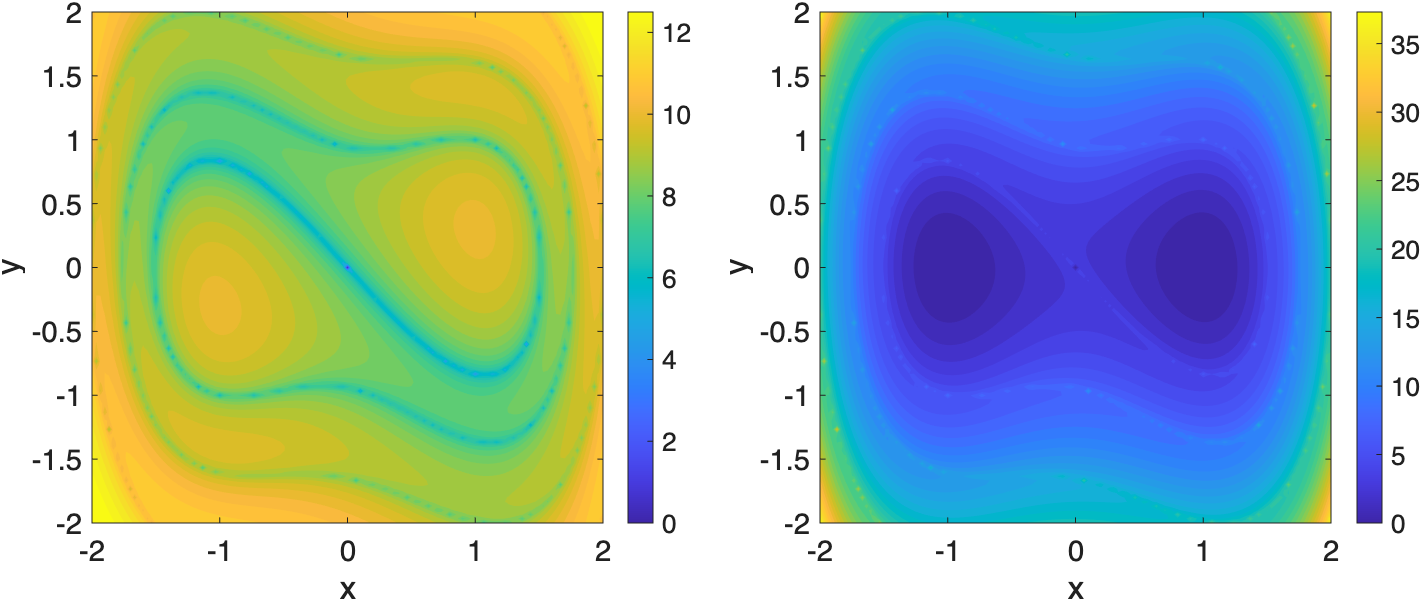
VII-B Stabilization of the inverted pendulum on a cart

We next consider stabilization of the inverted pendulum on a cart. This example highlights the local, online nature of the resolvent-based construction: at each state, the controller requires only the value and gradient of the supereigenfunction, which are computed numerically from short rollouts of the uncontrolled system. The approach does not need the global information about the supereigenfunction and hence the approach scale gracefully with the state space dimension. The state is $x=\begin{bmatrix}p&\dot{p}&\theta&\dot{\theta}\end{bmatrix}^{\top},$ where $p$ is the cart position and $\theta$ is measured from the upright configuration. The upright equilibrium is $x_{\mathrm{eq}}=\begin{bmatrix}0&0&0&0\end{bmatrix}^{\top}.$ The dynamics are

$\displaystyle\dot{x}_{1}$	$\displaystyle=x_{2},\qquad\dot{x}_{3}=x_{4},$
$\displaystyle\dot{x}_{2}$	$\displaystyle=\frac{u-b_{x}x_{2}+ms\big(lx_{4}^{2}+gc\big)}{{\cal D}(x)},$	(104)
$\displaystyle\dot{x}_{4}$	$\displaystyle=\frac{-uc+b_{x}x_{2}c-mlx_{4}^{2}cs-(M+m)gs-b_{\theta}x_{4}\,{\cal D}(x)}{l\,{\cal D}(x)},$

where $s=\sin x_{3}$ , $c=\cos x_{3}$ , and ${\cal D}(x)=M+ms^{2}$ . The parameters are $M=1.0,\;m=0.2,\;l=0.5,\;g=9.81.$ The supereigenfunction is approximated by the discrete resolvent

\varphi_{\lambda}(x)\approx\Delta t\sum_{j=0}^{H}e^{-\lambda j\Delta t}\,g_{p}(x_{j}),

(105)

using uncontrolled rollouts with $\Delta t=0.01,\;\;H=600,\;\;\lambda=1.$ The probe is chosen as

g_{p}(x)=b_{x}\dot{p}^{\,2}+b_{\theta}\dot{\theta}^{\,2}+\mu\left(\frac{k_{x}}{2}p^{2}+k_{\theta}(1-\cos\theta)\right),

(106)

with $b_{x}=0.10,\;b_{\theta}=0.05,\;k_{x}=1.0,\;k_{\theta}=5.0,\;\mu=2.0.$ This probe combines dissipative and potential terms and is aligned with the system’s mechanical structure. The gradient $\nabla\varphi_{\lambda}(x)$ is computed by centered finite differences. We first apply the QP controller in (66) with $\beta=-0.5,\;u_{\min}=-10,\;u_{\max}=10.$ From the initial condition $x_{0}=(0,0,0.95\pi,0)^{\top},$ the controller stabilizes the upright equilibrium, as shown in Fig. 5. We also test the gradient-based controller

u={\rm sat}_{[-10,10]}\left(-\frac{1}{2}{\cal K}_{g}\varphi_{\lambda}(x)\right),

(107)

where $g(x)$ denotes the control vector field. This controller also stabilizes the system from the same initial condition. Notably, the certificate is computed from rollout data, and only the control direction is used in feedback. A comparison of the evolution of the supereigenfunction along the system trajectory shows that it decays monotonically under the QP-based controller, whereas this monotonic decay is not observed for the gradient-based controller. This behavior is expected, as the QP formulation explicitly enforces a contracting inequality that guarantees asymptotic decay of the supereigenfunction along the closed-loop trajectory. The proposed approach for stabilizing controller design is scalable for system with large dimensional state space as the supereigenfunction are not computed globally but point-wise along the closed loop trajectory with rollouts.

VII-C 4D Duffing system with obstacle avoidance

Finally, we consider a four-dimensional system formed by two coupled Duffing oscillators:

	$\displaystyle\dot{x}_{1}$	$\displaystyle=y_{1},\qquad\dot{y}_{1}=-\delta y_{1}-\alpha(x_{1}-x_{2})-\beta x_{1}^{3}+u_{1},$
	$\displaystyle\dot{x}_{2}$	$\displaystyle=y_{2},\qquad\dot{y}_{2}=-\delta y_{2}-\alpha(x_{2}-x_{1})-\beta x_{2}^{3}+u_{2},$		(108)

with state $z=[x_{1},y_{1},x_{2},y_{2}]^{\top}$ , control $u=[u_{1},u_{2}]^{\top}$ , and parameters $\alpha=-1,\;\beta=1,\;\delta=0.3,\;u\in[-3,3]^{2}.$

VII-C1 Nominal stabilization

A nominal stabilizing controller is constructed from the resolvent-based certificate

\phi_{\mathrm{stab}}(z)=\int_{0}^{T_{1}}e^{-\lambda_{\rm stab}t}g(z(t))\,dt,\;\;g(z)=x_{1}^{2}+y_{1}^{2}+x_{2}^{2}+y_{2}^{2},

with $\lambda_{\rm stab}=1.0,\;\Delta t=0.05,\;H=120,\;T_{1}=H\Delta t$ . The gradient of $\phi_{\mathrm{stab}}$ is approximated by finite differences, and the nominal controller is

u_{\mathrm{nom}}=-{\rm sat}_{[-3,3]^{2}}\big({\cal K}_{g}\phi_{\mathrm{stab}}\big).

VII-C2 Safety filtering

Two unsafe regions are defined as spheres in ${\mathbb{R}}^{4}$ :

\mathcal{O}_{i}=\{z:\ \|z-c_{i}\|^{2}\leq r_{i}^{2}\},\qquad i=1,2,

with $c_{1}=(1.0,0.6,-0.6,0.5)^{\top},\;r_{1}=1.32,\;c_{2}=(-1.2,-0.7,0.9,-0.4)^{\top},\;r_{2}=1.5.$ Define the margins

m_{i}(z)=\|z-c_{i}\|^{2}-r_{i}^{2},

so that $m_{i}(z)>0$ corresponds to safe operation. For each obstacle we construct a safety certificate using the probe

g_{i}(z)=\frac{10}{1+\exp(\kappa m_{i}(z))},\qquad\kappa=25,

and

\phi_{\mathrm{safe},i}(z)=\int_{0}^{T_{2}}e^{-\lambda_{\rm safe}t}\,g_{i}(z(t))\,dt,

with $\lambda_{\rm safe}=1.0,\;\Delta t=0.05,\;H=180,\;T_{2}=H\Delta t.$ At each step, the control input is obtained from the QP

$\displaystyle\min_{u\in\mathbb{R}^{2}}\quad$	$\displaystyle\frac{1}{2}(u-u_{\mathrm{nom}})^{\top}R(u-u_{\mathrm{nom}})$
s.t.	$\displaystyle L_{f}\phi_{\mathrm{safe},i}(z)+L_{g}\phi_{\mathrm{safe},i}(z)\,u\leq-\alpha_{i}\phi_{\mathrm{safe},i}(z),$
	$\displaystyle u\in[-3,3]^{2},\;\;i=1,2,$	(109)

with $\alpha_{1}=\alpha_{2}=0.1,\;R=0.5I.$ The system is simulated for $T=10$ seconds from $z_{0}=[2.5,0.8,-2.0,0.6]^{\top}$ . The nominal controller drives the state toward the origin, while the safety filter modifies the control only when the trajectory approaches an obstacle. Safety is verified by

\min_{t\in[0,T]}m_{i}(z(t))>0,\qquad i=1,2.

For visualization, the trajectory is projected onto the $(x_{1},x_{2})$ and $(y_{1},y_{2})$ planes. This example illustrates simultaneous stabilization and safety enforcement in a higher-dimensional nonlinear system. It is important to emphasize that the minimum distances from the origin to obstacles $1$ and $2$ are approximately $0.08$ and $0.20$ , respectively. Despite these tight safety margins, the proposed control approach successfully steers the system to the origin while maintaining safety.

VII-D Synchronization of a Forced Duffing Oscillator

We consider a leader–follower pair of Duffing oscillators. The leader is driven by a sinusoidal input,

	$\displaystyle\dot{x}_{L}$	$\displaystyle=y_{L},$
	$\displaystyle\dot{y}_{L}$	$\displaystyle=-\delta y_{L}-\alpha x_{L}-\beta x_{L}^{3}+A_{L}\sin(\omega_{L}t),$		(110)

while the follower evolves as

	$\displaystyle\dot{x}_{F}$	$\displaystyle=y_{F},$
	$\displaystyle\dot{y}_{F}$	$\displaystyle=-\delta y_{F}-\alpha x_{F}-\beta x_{F}^{3}+u.$		(111)

The parameters are $\alpha=-1,\;\beta=1,\;\delta=0.2,\quad A_{L}=0.3,\;\omega_{L}=1,$ with simulation horizon $T=120$ s and step size $\Delta t=0.01$ . The initial conditions are chosen to be $z_{L}(0)=\begin{bmatrix}0.1&0.2\end{bmatrix}^{\top},\;z_{F}(0)=\begin{bmatrix}-0.1&-0.3\end{bmatrix}^{\top}$ and corresponds to initializing the system in two different potential wells of the oscillator. Let $e=z_{F}-z_{L}$ denote the synchronization error. A finite-horizon Gramian metric is computed along the forced leader trajectory,

M_{T_{g}}(x)=\int_{0}^{T_{g}}e^{-2\lambda\tau}Y(t,x)^{\top}QY(t,x)\,dt,

where $Y(t,x)=Ds^{L}_{t}(x)$ is the Jacobian evaluated along the trajectory of the leader system. The parameters are $\Delta t_{g}=0.02,\;H_{g}=500,\;\lambda=5,\;Q=I_{2}.$ The corresponding tangent-space certificate is $V_{\delta}(t)=e(t)^{\top}M_{T_{g}}(x)(t)e(t).$ The follower control is synthesized using a scalar quadratic program that enforces contraction of the certificate:

$\displaystyle\min_{u}\quad$	$\displaystyle\tfrac{1}{2}(u-u_{\rm nom})^{2}$	(112)
s.t.	$\displaystyle 2e^{\top}M_{T_{g}}(x)\big(f_{F}(z_{F})+Bu-f_{L}(z_{L},t)\big)$
	$\displaystyle\leq-\gamma\,e^{\top}M_{T_{g}}(x)e,$

where $B=[0\ \ 1]^{\top}$ , $u_{\rm nom}=0$ , $\gamma=2$ , and $u\in[-30,30]$ . This formulation yields a minimum-intervention control law that enforces decay of the tangent-space certificate. Simulation results show that the follower successfully synchronizes with the oscillatory leader, while the certificate $V_{\delta}(t)$ decreases along the trajectory, demonstrating contraction-based synchronization using Gramian supereigenfunction certificates.

VIII Conclusion and Future Direction

This paper introduced supereigenfunctions as an inequality-based generalization of Koopman eigenfunctions, providing an operator-theoretic framework for analyzing and controlling nonlinear systems through bounds and certificates. The key contribution is a shift in perspective: Koopman methods are used not to construct predictive models, but to construct certificates such as Lyapunov functions, Hamilton–Jacobi value functions, and safety constraints. We developed directional supereigenfunctions for contraction and incremental stability, and resolvent/Gramian constructions that enable computation directly from trajectory data. These results establish a bridge between Koopman operator theory and inequality-based control methods, while providing a scalable, data-driven alternative to PDE and SOS-based approaches.

References

[1] B. O. Koopman (1931) Hamiltonian systems and transformation in hilbert space. Proceedings of the national academy of sciences of the united states of america 17 (5), pp. 315. Cited by: §I.
[2] I. Mezić (2005) Spectral properties of dynamical systems, model reduction and decompositions. Nonlinear Dynamics 41, pp. 309–325. Cited by: §I.
[3] I. Mezić (2020) Spectrum of the Koopman operator, spectral expansions in functional spaces, and state-space geometry. Journal of Nonlinear Science 30 (5), pp. 2091–2145. Cited by: §I, §II-B.
[4] M. O. Williams, I. G. Kevrekidis, and C. W. Rowley (2015) A data–driven approximation of the Koopman operator: extending dynamic mode decomposition. Journal of Nonlinear Science 25 (6), pp. 1307–1346. Cited by: §I.
[5] M. Korda and I. Mezić (2018) On convergence of extended dynamic mode decomposition to the Koopman operator. Journal of Nonlinear Science 28 (2), pp. 687–710. Cited by: §I.
[6] E. Kaiser, J. N. Kutz, and S. L. Brunton (2017) Data-driven discovery of Koopman eigenfunctions for control. Bulletin of the American Physical Society 62. Cited by: §I.
[7] M. Korda and I. Mezić (2020) Optimal construction of Koopman eigenfunctions for prediction and control. IEEE Transactions on Automatic Control 65 (12), pp. 5114–5129. Cited by: §I.
[8] M. Korda and I. Mezić (2018) Linear predictors for nonlinear dynamical systems: Koopman operator meets model predictive control. Automatica 93, pp. 149–160. Cited by: §I.
[9] U. Vaidya, S. Narayanan, and P. Tallapragada (2025) When koopman meets hamilton and jacobi: linear operator formulation of nonlinear estimation. IEEE Transactions on Automatic Control. Cited by: §I.
[10] B. Huang and U. Vaidya (2018) Data-driven approximation of transfer operators: naturally structured dynamic mode decomposition. In 2018 Annual American Control Conference (ACC), pp. 5659–5664. Cited by: §I.
[11] B. Huang, X. Ma, and U. Vaidya (2018) Feedback stabilization using Koopman operator. In 2018 IEEE Conference on Decision and Control (CDC), pp. 6434–6439. Cited by: §I.
[12] U. Vaidya (2026) Discovering the Kalman-Bucy-Koopman filter. arXiv preprint arXiv:2606.30487. Cited by: §I.
[13] H. K. Khalil (1996) Nonlinear systems. Prentice Hall, New Jersey. Cited by: §I.
[14] M. G. Crandall, H. Ishii, and P. Lions (1992) User’s guide to viscosity solutions of second order partial differential equations. Bulletin of the American Mathematical Society 27 (1), pp. 1–67. Cited by: §I.
[15] L. C. Evans (2010) Partial differential equations. American Mathematical Society. Cited by: §I.
[16] E. D. Sontag (1999) Control-Lyapunov functions. In Open problems in mathematical systems and control theory, V. D. Blondel, E. D. Sontag, M. Vidyasagar, and J. C. Willems (Eds.), Comm. Control Engrg. Ser., pp. 211–216. Cited by: §I.
[17] E. D. Sontag (1998) Mathematical control theory. Springer. Cited by: §I.
[18] Z. Artstein (1983) Stabilization with relaxed controls. Nonlinear Analysis 7 (11), pp. 1163–1173. Cited by: §I.
[19] A. D. Ames, X. Xu, J. W. Grizzle, and P. Tabuada (2017) Control barrier function based quadratic programs for safety critical systems. IEEE Transactions on Automatic Control 62 (8), pp. 3861–3876. Cited by: §I.
[20] J. E. Slotine and W. Lohmiller (1998) On contraction analysis for nonlinear systems. Automatica 34 (6), pp. 683–696. Cited by: §I.
[21] V. I. Oseledets (1968) A multiplicative ergodic theorem. lyapunov characteristic numbers for dynamical systems. Trans. Moscow Math. Soc. 19, pp. 197–231. Cited by: §I, §IV-A2.
[22] D. Ruelle (1979) Ergodic theory of differentiable dynamical systems. Publications Mathématiques de l’IHÉS. Cited by: §I.
[23] P. A. Parrilo (2000) Structured semidefinite programs and semialgebraic geometry methods in robustness and optimization. Ph.D. Thesis, California Institute of Technology, Pasadena, CA. Cited by: §I.
[24] J. Moyalan, H. Choi, Y. Chen, and U. Vaidya (2021) Sum of squares based convex approach for optimal control synthesis. In 2021 29th Mediterranean Conference on Control and Automation (MED), pp. 1270–1275. Cited by: §I.
[25] J. Moyalan, H. Choi, Y. Chen, and U. Vaidya (2023) Data-driven optimal control via linear transfer operators: a convex approach. Automatica 150, pp. 110841. Cited by: §I.
[26] J. B. Lasserre, D. Henrion, C. Prieur, and E. Trélat (2008) Nonlinear optimal control via occupation measures and lmi-relaxations. SIAM journal on control and optimization 47 (4), pp. 1643–1666. Cited by: §I.
[27] U. Vaidya and D. T. Castro (2023) Data-driven stochastic optimal control via linear transfer operator. Accepted for Publication in IEEE TAC. Cited by: §I.
[28] A. Joglekar, C. Samak, T. Samak, V. N. Krovi, and U. Vaidya (2025) Expanding autonomous ground vehicle navigation capabilities through a multi-model parameterized Koopman framework. The International Journal of Robotics Research. Note: To appear / Early access Cited by: §I.
[29] C. V. Samak, T. V. Samak, A. S. Joglekar, and U. Vaidya (2024) Digital twins meet the Koopman operator: data-driven learning for robust autonomy. ICRA. Cited by: §I.
[30] D. Ha and J. Schmidhuber (2018) World models. NeurIPS. Cited by: §I.
[31] A. Lasota and M. Mackey (1994) Chaos, fractals, and noise: stochastic aspects of dynamics. Cited by: §II-B, §III-A.
[32] M. G. Krein and M. A. Rutman (1948) Linear operators leaving invariant a cone in a banach space. Uspekhi Matematicheskikh Nauk. Cited by: §III.
[33] R. D. Nussbaum (1986) Convexity and log convexity for the spectral radius. Linear Algebra and its Applications 73, pp. 59–122. Cited by: §III-C, §III.
[34] K. Engel and R. Nagel (2000) One-parameter semigroups for linear evolution equations. Springer. Cited by: §III-A, §III-C.
[35] A. Berman and R. J. Plemmons (1994) Nonnegative matrices in the mathematical sciences. SIAM. Cited by: §III-C.
[36] E. Seneta (2006) Non-negative matrices and markov chains. Springer. Cited by: §III-C.
[37] H. H. Schaefer (1974) Banach lattices and positive operators. Springer. Cited by: §III-C.

	$\displaystyle\mathcal{K}_{f}\varphi(x)$	$\displaystyle\leq 2L\\|x\\|+2L\\|x\\|^{2}$
		$\displaystyle\leq L(1+\\|x\\|^{2})+2L\\|x\\|^{2}$
		$\displaystyle\leq 3L(1+\\|x\\|^{2})=3L\varphi(x).$

	$\displaystyle\\|\varphi_{\lambda}-\varphi_{\lambda,T}\\|$	$\displaystyle\leq\int_{T}^{\infty}e^{-\lambda t}\\|U_{t}g\\|\,dt$
		$\displaystyle\leq M\\|g\\|\int_{T}^{\infty}e^{-(\lambda-\omega)t}\,dt,$		(45)