Residual Trajectory Distillation for
Generative Retrieval

Weihao Shen Affiliation: Institute of Artificial Intelligence, Beihang University, Beijing, China Affiliation: Meituan, Beijing, China Email: shenweihao@buaa.edu.cn Wei Chen Affiliation: Institute of Artificial Intelligence, Beihang University, Beijing, China Affiliation: Meituan, Beijing, China Email: chenwei23@buaa.edu.cn Fuwei Zhang Affiliation: Institute of Artificial Intelligence, Beihang University, Beijing, China Email: zhuangfuzhen@buaa.edu.cn Guojun Liu Affiliation: Meituan, Beijing, China Qingsong Hua Affiliation: Meituan, Beijing, China Wei Lin Affiliation: Meituan, Beijing, China Fuzhen Zhuang ^†^†thanks: Corresponding author. Affiliation: Institute of Artificial Intelligence, Beihang University, Beijing, China

Abstract

Generative retrieval has emerged as a general retrieval paradigm, representing items with discrete Semantic IDs (SIDs) and retrieving them through autoregressive identifier generation. When SIDs are constructed with residual quantization (RQ), standard retrieval training supervises only the selected codes and discards the residual trajectories that produce them. The same hard code can nevertheless arise from different preferences over competing codewords, while the residual trajectory also contains information about subsequent quantization decisions. As a result, hard SID supervision collapses distinct quantization behaviors into identical targets and leaves information available during indexing unused in retrieval training. We introduce ResTD, a Residual Trajectory Distillation framework that transfers this discarded indexing information into retrieval training. Treating the frozen RQ indexer as a process teacher, it distills residual-induced codeword preferences into SID-decoding states. This supervision recovers distinctions hidden by hard assignments and allows earlier decoder states to capture information about subsequent quantization decisions before the corresponding SID suffix is generated. In this way, richer information from SID construction is incorporated into retrieval learning while preserving the original retrieval index and inference procedure. Experiments on multilingual e-commerce retrieval show consistent improvements over strong baselines and matched training controls. Controlled comparisons show that residual-derived targets outperform the tested codebook-only soft targets. Representation probes further show that future codebook preferences become more recoverable from earlier decoder states. ResTD can also be readily extended beyond retrieval to generative recommendation. Code is available at: https://github.com/Nevaeh7/iclr2027_ResTD.git.

1 Introduction

Generative retrieval has emerged as a prominent paradigm that reformulates retrieval as sequence generation, producing identifiers of relevant documents or items from a query (De Cao et al., 2021; Tay et al., 2022; Wang et al., 2022; Sun et al., 2023; Zhang et al., 2025). A central challenge in this paradigm is constructing discrete identifiers that preserve useful semantic structure. Learned Semantic IDs (SIDs) have attracted substantial attention, with recent work focusing on their construction and use in generative retrieval (Zeng et al., 2024a; Li et al., 2024; Liu et al., 2026). Most existing generative retrieval methods (Rajput et al., 2023; Fu et al., 2026; Zhang et al., 2026b) use the final SID as the supervision target, as it directly serves as the retrieval address and is generated at inference. This outcome-level supervision captures only the selected discrete assignments. For RQ-based SIDs, the residuals produced during identifier construction encode finer-grained preferences over competing codewords that are not reflected in the final SID and thus remain unused in retrieval training.

Figure 1: ResTD uses the frozen RQ indexer as a process teacher, distilling current and future codebook preferences into SID-decoding states. The retrieval index and inference remain unchanged.

This information loss is particularly pronounced for residual-quantized identifiers. Residual quantization (RQ) constructs an SID progressively by selecting a codeword at each level and passing the remaining residual to the next (Gray, 1984; van den Oord et al., 2017; Lee et al., 2022; Rajput et al., 2023). The selected code alone does not fully characterize the residual that produced it. As illustrated in Figure 1, two residuals may induce different preferences over competing codewords while sharing the same selected code, making them indistinguishable under hard token supervision. Their relative distances and margins to alternative codewords can differ substantially within the same quantization cell. These distinctions also extend beyond the current level, since the remaining residual determines the input to subsequent quantization stages and influences later code selections. The trajectory therefore retains information about current preferences and subsequent quantization decisions. Hard SID supervision provides no signal to preserve this information in decoder states. Consequently, the final SID records the quantization outcomes but omits the fine-grained structure underlying their formation, creating an information gap between indexing and retrieval training.

Residual-distance distributions provide a natural way to recover information otherwise discarded by hard SID supervision (Hinton et al., 2015; Lee et al., 2022). Yet using them for retrieval is not straightforward. An SID is both a quantization outcome and an address in a fixed retrieval index. The preferences induced by residual geometry therefore need not align with the retrieval target. A nearby codeword may correspond to another item or an invalid path, and quantization proximity itself does not imply query relevance. Moreover, collision resolution may cause the stored SID to differ from the code preferred by the reconstructed residual. Directly distilling these preferences can therefore conflict with the discrete target used for retrieval. Residual supervision must preserve the informative structure exposed during quantization while remaining consistent with the stored retrieval address.

To satisfy these requirements, we introduce ResTD, a residual trajectory distillation framework that treats the frozen RQ indexer as a process teacher. ResTD transfers residual-induced codeword preferences into query-conditioned SID-decoding states, recovering distinctions obscured by hard assignments while remaining consistent with the stored SID. This consistency preserves the retrieval address and incorporates richer information from SID construction into retrieval learning without altering the original identifier space. Beyond the current quantization decision, ResTD further supervises earlier decoder states with preferences from subsequent quantization levels across multiple future horizons before the corresponding SID suffix enters the autoregressive context. Prior work has used future information to improve sequence representations through future-state matching or multi-token prediction (Serdyuk et al., 2018; Qi et al., 2020; Gloeckle et al., 2024). Here, item-conditioned codeword distributions serve as future targets that retain distinctions not expressed by future hard tokens alone. This encourages earlier decoder states to encode structure associated with the remaining identifier before those codes are generated, providing richer supervision for SID prediction.

We evaluate ResTD on the ESCI product-retrieval benchmark (Reddy et al., 2022) in English, Spanish, and Japanese. ResTD consistently outperforms strong baselines across all 15 reported evaluation settings. Controlled comparisons show benefits over future hard-target supervision, codebook-only targets, and shape-matched teachers from other items. Representation probes further show that future codebook preferences are more recoverable from earlier decoder states. We also extend ResTD to generative recommendation, where it consistently improves performance across multiple datasets.

Our contributions are threefold:

(i) We identify a gap between RQ-based SID construction and retrieval training, where hard SID supervision discards residual structure associated with current and subsequent quantization decisions.

(ii) We propose ResTD, which turns a frozen RQ indexer into a process teacher and transfers current and future residual-induced preferences from the indexing process into SID-decoding states while preserving the deployed retrieval addresses and autoregressive inference procedure.

(iii) ResTD improves retrieval and recommendation. Controls assess residual structure and correspondence between items and teachers; probes examine future preferences in early decoder states.

2 Related Work

Generative retrieval and learned identifiers. Generative retrieval autoregressively produces entity names, document spans, or discrete identifiers (De Cao et al., 2021; Bevilacqua et al., 2022; Tay et al., 2022; Wang et al., 2022). A major line of work develops identifiers preserving document or item semantics. GenRet learns discrete document tokenization (Sun et al., 2023), while TIGER constructs Semantic IDs with residual quantization (Rajput et al., 2023). LETTER and MERGE incorporate collaborative and relevance signals into identifier learning (Wang et al., 2024; Zhang et al., 2025). Beyond identifier construction, LTRGR introduces ranking-aware training (Li et al., 2024), while PAG, CaLIR, and PRO advance autoregressive search, latent intent modeling, and prefix retention, respectively (Zeng et al., 2024b; Zhang et al., 2026b; Chen et al., 2026). ResTD complements these directions by deriving supervision from residual quantization during the construction of a fixed RQ-based index, using additional indexing information that is discarded once the final SID is formed.

Distillation and codebook supervision. Knowledge distillation transfers information beyond hard labels through soft predictions, intermediate representations, generated sequences, or structural relations (Hinton et al., 2015; Kim and Rush, 2016; Romero et al., 2015; Park et al., 2019). In quantized generative models, RQ-Transformer derives soft code targets from residual distances (Lee et al., 2022). ETEGRec aligns sequence representations with item code distributions and reconstructed item embeddings (Liu et al., 2025), while TARQ aligns residual-to-code distributions for target-attention approximation (Li et al., 2026). SmartGR distills hierarchical SID predictions and beam-ranking preferences from a stronger recommender (Zhang et al., 2026c). ResTD instead treats the frozen RQ indexer itself as the teacher: residual preferences are reconstructed along stored SID paths and directly distilled into SID-decoding states without changing the underlying identifier space.

Future supervision. Future information has long been used to strengthen earlier sequence representations. Twin Networks regularize forward states using future context (Serdyuk et al., 2018); ProphetNet and multi-token prediction supervise a state with multiple subsequent tokens (Qi et al., 2020; Gloeckle et al., 2024); and recent work further explores compact future summaries as predictive targets (Mahajan et al., 2026). ResTD follows this line of work by using residual codebook distributions as structured future targets. Earlier decoder states are thereby explicitly supervised by both future SID assignments and codeword preferences at subsequent quantization levels.

Figure 2: Overview of ResTD. The frozen RQ indexer supplies residual-derived teacher distributions along stored SID paths; horizon-specific heads align decoder states with current and future targets.

3 Preliminaries: Residual-Quantized Retrieval

Residual-quantized indexing. Residual quantization (RQ) represents an item through successive vector quantization over level-specific codebooks (van den Oord et al., 2017; Lee et al., 2022; Rajput et al., 2023). Let ${\bm{x}}_{d}\in\mathbb{R}^{D}$ denote the representation of item $d$ , and let $\mathcal{C}_{t}=\{{\bm{c}}_{t,j}\}_{j=1}^{K_{t}}$ be the codebook at level $t$ . Starting from ${\bm{r}}_{0}={\bm{x}}_{d}$ , the $t$ -th quantization level selects the nearest codeword and updates the residual for the next level as follows:

y_{t}=\argmin_{j}\|{\bm{r}}_{t-1}-{\bm{c}}_{t,j}\|_{2}^{2},\qquad{\bm{r}}_{t}={\bm{r}}_{t-1}-{\bm{c}}_{t,y_{t}}.

(1)

After $L$ levels, the indexer yields the Semantic ID ${\bm{y}}(d)=(y_{1},\ldots,y_{L})$ and the residual trajectory $({\bm{r}}_{0},\ldots,{\bm{r}}_{L})$ . The SID records the discrete quantization path, while the residual trajectory retains the intermediate states that determine each codeword selection.

Autoregressive SID retrieval. Given a query $q$ , a generative retriever with parameters $\theta$ predicts the target SID autoregressively. Under teacher forcing, we use the standard sequence-generation objective for SID prediction (Sutskever et al., 2014; Tay et al., 2022)

\mathcal{L}_{\mathrm{SID}}=-\sum_{t=1}^{L}\log p_{\theta}(y_{t}\mid q,y_{<t}).

(2)

Let ${\bm{h}}_{t}$ denote the decoder state used to predict $y_{t}$ . In CaLIR (Zhang et al., 2026b), ${\bm{h}}_{1}$ corresponds to the final reasoning state and ${\bm{h}}_{2:L}$ to subsequent SID-decoding states. ResTD applies auxiliary supervision only to states that directly predict SID tokens.

Hard assignments and residual geometry. Equation 1 retains only the nearest-code assignment. Within the same quantization cell, however, residuals can have different distances and margins to the remaining codewords (Gray, 1984). Consequently, identical hard SID targets need not imply identical local codebook preferences. This distinction between the selected code and the residual geometry underlying the selection forms the basis of the supervision introduced next.

4 ResTD: Learning from the Indexing Process

ResTD uses the frozen RQ indexer as a structured teacher in the codebook geometry that defines the Semantic IDs. The supervision retains the residual-induced preferences available before each discrete code selection, recovering information that the selected code itself cannot express. The frozen codebooks provide a shared reference space: indexer residuals define teacher distributions over codewords, and projected decoder states define student distributions in the same space. We first align the two at the current quantization level and then extend the supervision across the remaining residual trajectory. Since the retrieval index remains fixed, each teacher target must stay consistent with the stored SID without altering the deployed identifier space. Figure 2 summarizes the framework.

4.1 Residual Behavioral Distillation

At quantization level $t$ , the residual ${\bm{r}}_{t-1}$ induces a complete set of distances to the codewords in $\mathcal{C}_{t}$ . Standard RQ compresses this geometry into the nearest-code assignment in Equation 1. ResTD instead retains the pre-assignment geometry through the teacher distribution

{\mathcal{Q}}_{t}(j\mid d)=\frac{\exp\!\left(-\|{\bm{r}}_{t-1}-{\bm{c}}_{t,j}\|_{2}^{2}/\tau_{T}\right)}{\sum_{m=1}^{K_{t}}\exp\!\left(-\|{\bm{r}}_{t-1}-{\bm{c}}_{t,m}\|_{2}^{2}/\tau_{T}\right)},

(3)

where $\tau_{T}$ controls the concentration of the distribution. Unlike the hard assignment $y_{t}$ , ${\mathcal{Q}}_{t}$ retains both the ordering and relative margins among competing codewords. In particular, for any pair $j,k$ ,

\log\frac{{\mathcal{Q}}_{t}(j\mid d)}{{\mathcal{Q}}_{t}(k\mid d)}=\frac{2{\bm{r}}_{t-1}^{\top}({\bm{c}}_{t,j}-{\bm{c}}_{t,k})+\|{\bm{c}}_{t,k}\|_{2}^{2}-\|{\bm{c}}_{t,j}\|_{2}^{2}}{\tau_{T}}.

(4)

Thus, two residuals assigned to the same hard code can induce different pairwise preferences over the remaining codebook. The teacher distribution captures this item-side quantization geometry; query relevance remains supervised by the original retrieval objective.

Let ${\bm{h}}_{t}$ denote the decoder state used to predict $y_{t}$ . We introduce a learnable projection $g_{0}:\mathbb{R}^{d_{h}}\rightarrow\mathbb{R}^{D}$ and score the projected state against the frozen codebook at level $t$ :

{\mathcal{P}}_{t,0}(j\mid q,d)=\mathrm{softmax}_{j}\!\left(-\frac{\|g_{0}({\bm{h}}_{t})-{\bm{c}}_{t,j}\|_{2}^{2}}{\tau_{S}}\right),

(5)

where $\tau_{S}$ is the student temperature. Teacher and student distributions are induced by distances to $\mathcal{C}_{t}$ and therefore share the codebook geometry. This permits comparison within the quantization space used to construct the SID. Residual Behavioral Distillation (RBD) minimizes the average teacher–student divergence in the frozen codebook space:

\mathcal{L}_{\mathrm{RBD}}=\frac{1}{L}\sum_{t=1}^{L}D_{\mathrm{KL}}\!\left({\mathcal{Q}}_{t}\,\|\,{\mathcal{P}}_{t,0}\right).

(6)

The resulting objective also admits a geometric interpretation. For a fixed teacher, its gradient with respect to the projected state is

\nabla_{g_{0}({\bm{h}}_{t})}D_{\mathrm{KL}}\!\left({\mathcal{Q}}_{t}\,\|\,{\mathcal{P}}_{t,0}\right)=\frac{2}{\tau_{S}}\left(\sum_{j}{\mathcal{P}}_{t,0}(j\mid q,d){\bm{c}}_{t,j}-\sum_{j}{\mathcal{Q}}_{t}(j\mid d){\bm{c}}_{t,j}\right).

(7)

RBD therefore aligns the codebook-weighted expectations induced by the decoder state and the indexer residual. In practice, ${\mathcal{Q}}_{t}$ is replaced by the collision-aware teacher introduced in Section 4.3, and only valid SID positions contribute to the loss. The original SID objective remains unchanged, so the retriever is jointly supervised by the target identifier and the geometry underlying its construction.

4.2 Multi-Horizon Residual Trajectory Distillation

Current-level RBD transfers the quantization preference associated with the code currently being generated. The residual trajectory also captures the subsequent decisions required to complete the SID. ResTD uses these subsequent preferences to supervise earlier decoder states before the corresponding suffix codes enter the autoregressive context. We introduce $H$ horizon-specific projections $\{g_{s}\}_{s=0}^{H-1}$ . For state ${\bm{h}}_{t}$ and horizon offset $s$ , the target quantization level is $t+s$ , with residual state ${\bm{r}}_{t+s-1}$ and codebook $\mathcal{C}_{t+s}$ . The corresponding teacher and student distributions are defined as follows:

	$\displaystyle{\mathcal{Q}}_{t,s}(j\mid d)$	$\displaystyle=\mathrm{softmax}_{j}\!\left(-\frac{\\|{\bm{r}}_{t+s-1}-{\bm{c}}_{t+s,j}\\|_{2}^{2}}{\tau_{T}}\right),$		(8)
	$\displaystyle{\mathcal{P}}_{t,s}(j\mid q,d)$	$\displaystyle=\mathrm{softmax}_{j}\!\left(-\frac{\\|g_{s}({\bm{h}}_{t})-{\bm{c}}_{t+s,j}\\|_{2}^{2}}{\tau_{S}}\right).$		(9)

For position $t$ , valid offsets satisfy $0\leq s<H_{t}$ , where $H_{t}=\min(H,L-t+1)$ . The case $s=0$ recovers current-level RBD, while $s>0$ associates the same decoder state with preferences from later quantization levels. The resulting supervision is triangular: early decoder states are constrained by a longer suffix of the residual trajectory, whereas the number of valid future targets decreases toward the end of the SID. We aggregate all valid state–horizon pairs using the normalized objective:

\mathcal{L}_{\mathrm{RT}}=\frac{1}{{\mathcal{Z}}}\sum_{t=1}^{L}\sum_{s=0}^{H_{t}-1}m_{t+s}\rho^{s}D_{\mathrm{KL}}\!\left(\widetilde{{\mathcal{Q}}}_{t,s}\,\|\,{\mathcal{P}}_{t,s}\right),\qquad{\mathcal{Z}}=\sum_{t=1}^{L}\sum_{s=0}^{H_{t}-1}m_{t+s}\rho^{s},

(10)

where $m_{t+s}$ masks invalid target positions and $0<\rho\leq 1$ discounts increasingly distant horizons. For each offset $s$ , the normalized trajectory mass used by the objective is

w_{s}=\frac{\rho^{s}\sum_{t=1}^{L-s}m_{t+s}}{{\mathcal{Z}}},\qquad\sum_{s=0}^{H-1}w_{s}=1.

(11)

When all positions are valid, this reduces to $w_{s}=(L-s)\rho^{s}/\sum_{u=0}^{H-1}(L-u)\rho^{u}$ . The horizon therefore determines both the range and relative weighting of future supervision. When $H=1$ , Equation 10 reduces to current-level RBD. The target $\widetilde{{\mathcal{Q}}}_{t,s}$ preserves the relative preferences among competing codewords in addition to the selected future code. These soft targets separate items that share the same future assignment and encourage earlier decoder states to encode future codebook preferences before the corresponding SID suffix is generated.

4.3 Collision-Aware Teacher Construction

Residual supervision must remain consistent with the SID stored in the retrieval index. Collision resolution can modify one or more nearest-code assignments to avoid duplicate identifiers, so a residual trajectory computed from the original RQ decisions need not follow the final retrieval path. We therefore reconstruct the trajectory along the stored SID. Given ${\bm{y}}^{\mathrm{final}}=(y_{1}^{\mathrm{final}},\ldots,y_{L}^{\mathrm{final}})$ , we initialize ${\bm{r}}_{0}={\bm{x}}_{d}$ and recursively compute ${\bm{r}}_{t}={\bm{r}}_{t-1}-{\bm{c}}_{t,y_{t}^{\mathrm{final}}}$ . The resulting residual states are consequently defined on the same discrete path as the retrieval target. Path reconstruction alone does not guarantee agreement between residual geometry and the stored code. At a given target, let $q_{y}$ denote the uncorrected probability of the stored code and $q_{\max}$ the largest probability among competing codes. We seek the smallest interpolation toward the stored assignment that enforces the target margin $\delta$ for each state–horizon pair:

\epsilon_{t,s}^{\star}=\min_{\alpha\in[0,1]}\alpha\quad\mathrm{s.t.}\quad(1-\alpha)q_{y}+\alpha\geq(1-\alpha)q_{\max}+\delta.

(12)

For each state–horizon pair, the corrected teacher distribution over the target codebook is

\widetilde{{\mathcal{Q}}}_{t,s}(j)=(1-\epsilon_{t,s}){\mathcal{Q}}_{t,s}(j)+\epsilon_{t,s}\,\mathbf{1}\!\left[j=y_{t+s}^{\mathrm{final}}\right].

(13)

Solving Equation 12 gives the closed-form correction required to enforce the stored-code margin:

\epsilon_{t,s}=\max\!\left\{\epsilon,\,\left[\frac{q_{\max}-q_{y}+\delta}{1-q_{y}+q_{\max}}\right]_{0}^{1}\right\},

(14)

where $[\cdot]_{0}^{1}$ clips to $[0,1]$ and $\epsilon$ is the minimum mixing weight. The correction is therefore the minimum adaptive perturbation, subject to the floor $\epsilon$ , required to make the stored code preferred by the teacher. Since every non-target probability is multiplied by the same factor $1-\epsilon_{t,s}$ , their pairwise ratios remain unchanged whenever $\epsilon_{t,s}<1$ . The procedure thus restores consistency with the fixed SID while preserving the residual-induced preference structure among alternatives.

Table 1: Overall ESCI retrieval results (%) across sparse, dense, and generative methods. ResTD reports three-seed means. Relative improvements compare with the strongest baseline in each column.

Sparse retrieval
	ESCI-US					ESCI-ES					ESCI-JP
Model	R@5	R@10	R@100	N@10	N@100	R@5	R@10	R@100	N@10	N@100	R@5	R@10	R@100	N@10	N@100
BM25 (FnT IR’09)	4.02	5.84	14.08	5.64	8.11	4.13	6.15	16.21	7.45	10.20	4.70	7.96	16.73	8.63	11.25
Dense retrieval
DPR (EMNLP’20)	5.54	8.93	29.30	8.17	15.55	5.24	7.08	25.27	8.52	14.33	4.18	7.26	23.84	8.98	14.73
MPNet (NeurIPS’20)	2.76	4.58	15.30	4.12	9.83	2.53	4.02	13.27	5.87	8.91	1.13	1.97	5.58	1.79	2.82
Sentence-T5 (ACL’22)	4.63	6.97	24.59	6.84	11.58	–	–	–	–	–	–	–	–	–	–
Sentence-mT5 (COLING’24)	–	–	–	–	–	5.44	8.68	30.04	8.42	15.09	5.69	8.73	29.01	9.19	15.70
BGE-M3 (ACL’24)	6.59	9.82	32.29	9.91	16.77	5.71	9.07	28.75	9.76	16.02	5.14	8.92	27.93	10.12	17.02
LaSER (SIGIR’26)	6.52	10.23	35.37	8.19	15.74	5.28	8.40	32.22	8.69	16.16	5.88	8.78	28.66	9.28	15.53
Generative retrieval
DSI_naive (NeurIPS’22)	0.42	1.74	2.03	0.32	0.99	0.28	0.94	1.83	0.77	1.60	0.19	0.24	1.35	0.21	1.11
DSI_semantic (NeurIPS’22)	3.74	6.02	20.69	6.24	10.60	4.27	7.13	21.63	9.92	14.23	4.08	7.40	23.90	9.15	14.58
TIGER (NeurIPS’23)	4.79	7.84	25.98	7.24	12.68	3.83	7.31	25.03	8.72	14.51	4.67	7.98	25.89	9.67	15.52
Hi-Gen (ICDM’24)	3.13	4.97	15.91	5.25	8.55	2.97	5.65	20.23	7.06	11.85	3.36	6.40	21.66	7.73	12.86
LTRGR (AAAI’24)	2.88	4.71	13.70	4.48	7.82	5.13	8.23	27.92	9.26	15.42	5.24	8.37	26.79	10.01	16.93
RIPOR (WWW’24)	5.05	8.35	26.80	7.92	13.75	3.49	7.12	23.03	7.94	13.82	5.02	8.18	27.87	9.92	17.28
MERGE (ACL’25)	5.68	9.26	29.74	9.05	15.17	5.80	9.25	30.86	10.20	17.45	5.21	8.90	27.64	10.95	17.60
CaLIR (arXiv’26)	7.50	12.69	37.40	11.12	18.79	6.03	10.48	34.15	12.43	19.88	6.05	9.77	30.89	11.77	18.42
CAT-ID² (WSDM’26)	6.11	8.89	29.03	8.96	14.53	5.70	9.34	31.44	10.68	18.01	5.36	8.87	28.82	10.34	17.14
FORGE (KDD’26)	5.59	9.26	35.11	8.50	16.21	4.87	8.29	28.42	9.99	16.66	3.88	6.58	24.06	8.27	14.22
HGRec (ICML’26)	6.70	11.41	34.61	10.19	17.32	5.76	9.60	31.56	11.37	18.32	3.78	6.18	24.37	8.40	13.83
ResTD	9.28	14.34	39.58	12.99	20.79	6.86	11.76	35.38	14.22	21.54	7.61	11.63	32.86	14.18	20.79
Rel. Improv. (%)	+23.73	+13.00	+5.83	+16.82	+10.64	+13.76	+12.21	+3.60	+14.40	+8.35	+25.79	+19.04	+6.38	+20.48	+12.87

4.4 Training and Inference

ResTD augments the original generative retrieval objective with residual trajectory distillation:

\mathcal{L}=\mathcal{L}_{\mathrm{GR}}+\lambda(u)\mathcal{L}_{\mathrm{RT}},\qquad\lambda(u)=\lambda_{\max}\min\!\left(1,\frac{u}{u_{\mathrm{warm}}}\right),

(15)

where $u$ is the optimization step and $u_{\mathrm{warm}}$ controls a linear warmup of the trajectory objective. In our CaLIR instantiation, $\mathcal{L}_{\mathrm{GR}}$ is unchanged and contains the original SID-generation and latent-reasoning objectives. The RQ indexer and codebooks remain fixed throughout training, while the retriever and horizon-specific projections are optimized jointly. During continuation training, the contribution of the trajectory objective is bounded relative to the SID objective so that residual supervision remains auxiliary to the retrieval target. At inference, the residual teachers and projection functions are removed. Retrieval therefore uses the original SID-generation distribution and trie-constrained autoregressive search, with no modification to the retrieval index or inference procedure.

5 Experiments

We evaluate ResTD through seven research questions: RQ1: How does the method compare with sparse, dense, and generative retrieval approaches? RQ2: How do residual supervision, multi-horizon distillation, and collision-aware teachers affect retrieval under matched settings? RQ3: Which teacher target properties contribute to retrieval gains? RQ4: Do learned decoder states encode current and future codebook preferences from the indexer? RQ5: How do teacher disagreement and relevant-item counts relate to retrieval gains? RQ6: Does residual trajectory supervision generalize to generative recommendation? RQ7: How can the advantage of ResTD be understood intuitively?

5.1 Experimental Setup

(1) Datasets. We evaluate ResTD on ESCI-US, ESCI-ES, and ESCI-JP (English, Spanish, and Japanese) from the Shopping Queries Dataset (ESCI), a large-scale multilingual product retrieval benchmark (Reddy et al., 2022), following the filtering and splits of Zhang et al. (2026b). (2) Baselines. We compare against sparse (BM25), dense (DPR, MPNet, Sentence-T5, Sentence-mT5, BGE-M3, and LaSER), and generative retrievers (DSI, TIGER, Hi-Gen, LTRGR, RIPOR, CAT-ID², MERGE, FORGE, HGRec, and CaLIR). The overall comparison includes published results under their original training protocols. Controlled comparisons start from the same reproduced CaLIR model under matched training and evaluation settings: continued fine-tuning (Base-FT), current-level RBD ( $H=1$ ), multi-horizon ResTD, future hard-SID supervision, shuffled-teacher variants, full-output distillation, and non-target output alignment. (3) Implementation Details. We use T5-base for ESCI-US and mT5-base for ESCI-ES/JP. The SID index has four quantization levels with 256 codewords each. Unless otherwise specified, $H=4$ , $\lambda_{\max}=0.1$ , $\tau_{T}=\tau_{S}=0.2$ , $\rho=0.7$ , and the collision-correction floor $\epsilon=0.1$ . Each controlled continuation uses 1,200 updates, effective batch size 128, learning rate $10^{-5}$ , and paired seeds 42, 2027, and 2028. Retrieval uses trie-constrained beam search with beam size 100. We report Recall@5/10/100 and NDCG@10/100 on the percentage scale. Further experimental details and hyperparameter sensitivity appear in Appendices A and C.7.

5.2 Experimental Results and Discussion

Main Experimental Results (RQ1). Table 1 shows that our method achieves the best results on every reported metric across ESCI-US, ESCI-ES, and ESCI-JP, consistently outperforming sparse, dense, and generative retrieval baselines. Our advantage is most pronounced at early ranks. Higher Recall and NDCG at these cutoffs show that ResTD brings more relevant items to the top of the retrieved list and improves their ordering. Recall@100 also increases in every dataset, indicating that our method combines stronger early ranking with broader coverage of relevant items. The gains over CaLIR, the strongest baseline, demonstrate the value of our residual trajectory supervision for generative retrieval. Our method enriches SID prediction with preferences over competing codewords, transferring information from identifier construction into query-conditioned retrieval learning. Our method consistently delivers these gains in English, Spanish, and Japanese using the same distillation hyperparameters. ResTD turns residual information from SID construction into more effective query-to-identifier prediction. Dataset preparation, baseline settings, relevance judgments, and the exact SID-level evaluation protocol for multilingual product retrieval are detailed in Appendix A.

Matched Training Objectives (RQ2). Table 2

Table 2: Matched ESCI training objectives under a shared 1,200-update budget. Entries are mean ± sample standard deviation across three paired seeds; bold marks each column’s highest mean overall.

	ESCI-US				ESCI-ES				ESCI-JP
Training objective	R@10	R@100	N@10	N@100	R@10	R@100	N@10	N@100	R@10	R@100	N@10	N@100
Base-FT	12.82±0.16	37.60±0.13	11.25±0.11	18.92±0.15	10.55±0.15	34.22±0.11	12.53±0.12	19.95±0.09	9.85±0.03	30.98±0.07	11.90±0.17	18.55±0.08
RBD (H=1)	13.23±0.10	38.20±0.08	11.78±0.05	19.44±0.13	10.84±0.11	34.46±0.09	12.98±0.08	20.30±0.10	10.29±0.06	31.48±0.14	12.50±0.09	19.10±0.07
Full-output KD	13.15±0.07	38.10±0.13	11.69±0.10	19.35±0.09	10.80±0.05	34.40±0.11	12.91±0.06	20.20±0.14	10.22±0.09	31.39±0.08	12.39±0.11	18.99±0.12
ResTD (H=2)	13.77±0.05	38.83±0.14	12.32±0.09	20.08±0.07	11.28±0.10	34.91±0.08	13.55±0.12	20.86±0.11	10.95±0.07	32.04±0.13	13.24±0.06	19.83±0.09
RBD + future hard SID (H=4)	13.56±0.09	38.68±0.07	12.18±0.08	19.93±0.13	11.16±0.04	34.81±0.05	13.40±0.10	20.71±0.15	10.81±0.03	31.96±0.11	13.12±0.07	19.72±0.16
Hard SID targets (H=4)	13.10±0.08	38.12±0.12	11.70±0.06	19.30±0.10	10.78±0.09	34.40±0.07	12.84±0.11	20.19±0.13	10.20±0.05	31.39±0.15	12.35±0.08	18.98±0.11
Shuffled ResTD (H=4)	12.86±0.05	37.68±0.11	11.22±0.12	18.95±0.03	10.51±0.06	34.10±0.04	12.60±0.14	19.92±0.03	9.89±0.06	31.02±0.12	11.88±0.13	18.59±0.07
Non-target output alignment	13.07±0.06	38.00±0.11	11.66±0.12	19.25±0.07	10.77±0.10	34.39±0.14	12.88±0.09	20.16±0.12	10.19±0.08	31.35±0.13	12.34±0.06	18.93±0.10
ResTD (H=4)	14.34±0.04	39.58±0.11	12.99±0.07	20.79±0.05	11.76±0.04	35.38±0.13	14.22±0.07	21.54±0.12	11.63±0.17	32.86±0.09	14.18±0.08	20.79±0.05

compares our supervision objectives across three paired seeds under the same training budget. Current-level RBD ( $H=1$ ) improves every reported metric over Base-FT and outperforms full-output KD with the same teacher, demonstrating the benefit of distilling residual preferences into decoder states. Extending supervision to $H=2$ and then $H=4$ yields progressive gains across all metrics and locales. Our multi-horizon formulation thus benefits from information at increasingly distant quantization levels. ResTD also surpasses RBD + future hard SID under matched horizon and supervision weights, improving the ranking and coverage of relevant items. This comparison establishes the value of future codeword preferences beyond future hard labels. Shuffled teachers yield retrieval scores close to Base-FT in all three locales. Collision-aware correction further improves Recall@100 and NDCG@10 in every locale by aligning residual preferences with the stored identifiers. The gains persist across moderate correction floors, with the default attaining the highest observed means. Appendix C.3 defines the output-space controls, and Appendix C.6.2 details the correction rule and sensitivity to the correction strength.

Refer to caption — Figure 3: Probe KL reduction (%) for ResTD ( $H=4$ ) over RBD ( $H=1$ ). Diagonal cells are current targets; rightward cells are future targets.

Dissecting Teacher Targets (RQ3). Table 3 shows that our teacher attains the highest mean score on every metric across all ESCI locales. We study controls that preserve different combinations of assigned codes, distributional shape, codeword preferences, and item–teacher correspondence at current and future levels. Code-conditioned residual distributions outperform both future hard-SID supervision and codebook-only targets, indicating that residual statistics carry useful supervision beyond hard assignments and codebook distances. Keeping the correspondence between codewords and their teacher probabilities also improves retrieval over non-target permutation, which preserves the probability profile but changes its association with codewords. Shape-matched teachers drawn from other items still yield substantial gains over Base-FT, showing that residual supervision captures structure shared across items. ResTD improves further on every reported metric when each item retains its own residual-induced preferences. Across these controls, residual geometry provides useful supervision over competing codewords, while item-specific preferences contribute an additional retrieval gain. Appendix C.2 gives the control constructions, matching quality, and retrieval results.

Table 3: Retrieval performance of ResTD and teacher-target controls on ESCI (%) across three paired seeds. Values are mean ± SD; bold marks each column’s highest mean; unm. denotes unmatched.

Teacher objective	Hard	Shape	Real	Pair	R@10	R@100	N@10	N@100	R@10	R@100	N@10	N@100	R@10	R@100	N@10	N@100
					ESCI-US				ESCI-ES				ESCI-JP
Base-FT	$\checkmark$	–	–	–	12.82±0.16	37.60±0.13	11.25±0.11	18.92±0.15	10.55±0.15	34.22±0.11	12.53±0.12	19.95±0.09	9.85±0.03	30.98±0.07	11.90±0.17	18.55±0.08
Shuffled ResTD	×	unm.	$\checkmark$	×	12.86±0.05	37.68±0.11	11.22±0.12	18.95±0.03	10.51±0.06	34.10±0.04	12.60±0.14	19.92±0.03	9.89±0.06	31.02±0.12	11.88±0.13	18.59±0.07
RBD + future hard SID	$\checkmark$	–	–	–	13.56±0.09	38.68±0.07	12.18±0.08	19.93±0.13	11.16±0.04	34.81±0.05	13.40±0.10	20.71±0.15	10.81±0.03	31.96±0.11	13.12±0.07	19.72±0.16
Codebook-only (H=4)	$\checkmark$	–	×	×	13.48±0.11	38.55±0.06	12.05±0.14	19.81±0.03	10.98±0.11	34.65±0.13	13.22±0.12	20.51±0.08	10.63±0.14	31.76±0.09	12.95±0.15	19.51±0.16
Code-conditioned mean	$\checkmark$	agg.	×	×	13.90±0.08	39.03±0.15	12.50±0.10	20.27±0.16	11.39±0.06	35.00±0.08	13.66±0.03	20.97±0.13	11.09±0.13	32.24±0.10	13.47±0.05	20.05±0.15
Same-code + entropy-bin shuffle	$\checkmark$	coarse	$\checkmark$	×	13.82±0.07	38.96±0.10	12.44±0.06	20.22±0.11	11.29±0.11	34.89±0.07	13.60±0.09	20.91±0.12	11.03±0.04	32.17±0.13	13.44±0.10	20.03±0.05
Non-target permutation	$\checkmark$	exact	×	×	13.76±0.10	38.86±0.16	12.36±0.15	20.12±0.09	11.29±0.04	34.93±0.15	13.54±0.12	20.84±0.06	10.96±0.04	32.11±0.05	13.31±0.10	19.89±0.12
Shape-matched teacher swap	$\checkmark$	near	$\checkmark$	×	14.16±0.10	39.36±0.07	12.79±0.03	20.58±0.11	11.61±0.11	35.23±0.03	14.00±0.05	21.31±0.07	11.41±0.04	32.61±0.07	13.90±0.09	20.49±0.17
ResTD (H=4)	$\checkmark$	exact	$\checkmark$	$\checkmark$	14.34±0.04	39.58±0.11	12.99±0.07	20.79±0.05	11.76±0.04	35.38±0.13	14.22±0.07	21.54±0.12	11.63±0.17	32.86±0.09	14.18±0.08	20.79±0.05

Representation Alignment (RQ4). We fit matched-capacity probes to frozen retrievers to recover collision-corrected teacher distributions from decoder states. Across conditions, query splits, probe architecture, initialization, and fitting procedure are fixed for the three retriever seeds, with a separate probe for each target offset. Figure 4 shows that ResTD ( $H=4$ ) reduces KL relative to current-level RBD ( $H=1$ ) at every future state–target pair across all three locales, with relative reductions of 5.3–13.8%. In contrast, reductions on current targets remain small, at 0.1–0.3%. The largest reduction in each locale occurs for the longest-horizon pair, where the first decoder state is probed against the fourth-level teacher distribution. This pattern localizes the effect of multi-horizon supervision to future codebook information: later-level preferences become substantially more recoverable from earlier decoder states, while current-target probe performance remains stable. Matched retrieval results are reported in Section 5.2, and probe specifications are provided in Appendix C.4.

Retrieval Gains across Query Groups (RQ5). We study how the gains from ResTD vary with disagreement among the teachers associated with relevant items. Figure 4 partitions multi-positive queries by first-level teacher JS divergence and reports the corresponding changes in Recall@100 and NDCG@10. On ESCI-US and ESCI-JP, improvements over both Base-FT and RBD ( $H=1$ ) increase with teacher disagreement, with the largest gains appearing in the high-disagreement group. On ESCI-ES, NDCG@10 gains peak in the intermediate-disagreement group. Across locales, stratified trends remain metric dependent, indicating no uniform gain pattern from disagreement. Controlling for the number of relevant items and initial query difficulty preserves positive associations on US and JP; the ES confidence intervals span zero. These query-level comparisons characterize dataset- and metric-specific associations between teacher disagreement and retrieval gains. Detailed teacher-disagreement statistics, disagreement-stratified gains, and adjusted analyses are reported in Appendix C.5.

Table 4: Generative recommendation results (%). ResTD uses TIGER as its backbone; improvement is relative to the best baseline per column.

Model	B-Shop		I-Shop		Yelp
Model	R@10	N@10	R@10	N@10	R@10	N@10
SASRec	5.88	3.13	9.47	6.90	2.96	1.52
BigRec	2.99	1.98	5.76	4.91	1.69	1.42
P5-SID	5.84	3.35	9.64	7.30	3.24	1.70
P5-CID	5.97	3.47	9.87	7.51	3.47	1.81
LETTER	6.72	3.64	11.22	8.31	4.26	2.31
TIGER	6.10	3.31	10.58	7.97	4.07	2.13
ETEGRec	6.15	3.35	11.06	8.10	4.15	2.14
ResTD	7.28	4.00	11.42	8.45	4.87	2.66
Improv. (%)	+8.33	+9.89	+1.78	+1.68	+14.32	+15.15

Generative Recommendation (RQ6). We apply ResTD to TIGER for history-conditioned next-item recommendation, using the frozen RQ tokenizer to supervise decoder states predicting semantic item codes. Table 4 reports Recall@10 and NDCG@10 on Beauty (B-Shop), Instruments (I-Shop), and Yelp. ResTD achieves the best performance across all dataset–metric settings, improving over strong baselines on e-commerce and non-e-commerce benchmarks. Gains are consistently strongest on B-Shop and Yelp, and positive across both I-Shop metrics. The results demonstrate that residual trajectory supervision extends beyond ESCI retrieval and provides effective signals for TIGER-based generative recommendation. Component effects are examined through retrieval experiments. Implementation details are provided in Appendix A.5.

Qualitative Analysis (RQ7). Figure 5 illustrates how ResTD improves retrieval by preserving promising identifier paths during generation. In the Casio example, the baseline prunes the target identifier early, whereas ResTD retains the complete path and improves the ranking of the target item. Similar behavior is observed for the complementary products in the US and JP examples, where ResTD maintains relevant candidates through later decoding steps and improves ranking quality. These examples demonstrate the benefit of residual trajectory supervision. Future quantization preferences provide additional guidance for early identifier generation, allowing relevant items to remain reachable during autoregressive retrieval. Additional examples are provided in Appendix D.

6 Conclusion

We introduced ResTD, a residual trajectory distillation framework that transfers current and future codebook preferences from a frozen RQ indexer into query-conditioned decoder states, enriching hard SID supervision and preserving the index and autoregressive inference. Across three ESCI locales, ResTD consistently outperforms continued training, current-level RBD, and future hard-SID supervision under matched settings. Controlled comparisons and representation probes support the value of residual-derived targets and improved access to future codebook information from early decoder states. Results on Beauty, Instruments, and Yelp extend ResTD to generative recommendation.

AI use statement

We used generative AI solely as a writing aid to refine the wording and improve the readability of the manuscript. We did not use it to formulate the research questions, design the methodology or experiments, or analyze and interpret the results. We reviewed all AI-assisted revisions and take full responsibility for the final version of the paper.

Ethics statement

We have reviewed the potential ethical implications of this work and do not identify any particular ethical issues that warrant additional discussion.

Reproducibility statement

To facilitate reproducibility, we provide detailed descriptions of the proposed method, experimental configuration, and evaluation procedure in the main paper and appendix. The source code and relevant implementation details are also made available through our GitHub repository to support independent reproduction of the reported results.

References

Bevilacqua et al. (2022) M. Bevilacqua, G. Ottaviano, P. Lewis, W. Yih, S. Riedel, and F. Petroni Autoregressive search engines: generating substrings as document identifiers. In NeurIPS, Cited by: §2.
Chen et al. (2024) J. Chen, S. Xiao, P. Zhang, K. Luo, D. Lian, and Z. Liu M3-Embedding: multi-linguality, multi-functionality, multi-granularity text embeddings through self-knowledge distillation. In Findings of ACL, Cited by: 5th item.
Chen et al. (2026) Y. Chen, Z. Wang, Y. Tang, Y. Zhao, M. de Rijke, and Z. Ren Closing the indexing-decoding gap in multimodal generative retrieval via prefix retention optimization. CoRR. Cited by: §2.
De Cao et al. (2021) N. De Cao, G. Izacard, S. Riedel, and F. Petroni Autoregressive entity retrieval. In ICLR, Cited by: §1, §2.
Fu et al. (2026) K. Fu, T. Zhang, S. Xiao, Z. Wang, X. Zhang, C. Zhang, Y. Yan, J. Zheng, X. Kong, S. Zhang, K. Kuang, and Y. Jiang FORGE: forming semantic identifiers for generative retrieval in industrial datasets. In KDD, Cited by: 9th item, §1.
Gloeckle et al. (2024) F. Gloeckle, B. Youbi Idrissi, B. Rozière, D. Lopez-Paz, and G. Synnaeve Better & faster large language models via multi-token prediction. In ICML, Cited by: §1, §2.
Gray (1984) R. M. Gray Vector quantization. IEEE ASSP Mag.. Cited by: §B.1, §1, §3.
Hinton et al. (2015) G. Hinton, O. Vinyals, and J. Dean Distilling the knowledge in a neural network. CoRR. Cited by: §1, §2.
Jin et al. (2026) J. Jin, Y. Zhang, M. Li, D. Long, P. Xie, Y. Zhu, and Z. Dou Internalizing explicit reasoning into latent space for dense retrieval. In SIGIR, Cited by: 6th item.
Karpukhin et al. (2020) V. Karpukhin, B. Oguz, S. Min, P. Lewis, L. Wu, S. Edunov, D. Chen, and W. Yih Dense passage retrieval for open-domain question answering. In EMNLP, Cited by: 1st item.
Kim and Rush (2016) Y. Kim and A. M. Rush Sequence-level knowledge distillation. In EMNLP, Cited by: §2.
Lee et al. (2022) D. Lee, C. Kim, S. Kim, M. Cho, and W. Han Autoregressive image generation using residual quantization. In CVPR, Cited by: §1, §1, §2, §3.
Li et al. (2024) Y. Li, N. Yang, L. Wang, F. Wei, and W. Li Learning to rank in generative retrieval. In AAAI, Cited by: 5th item, §1, §2.
Li et al. (2026) Y. Li, Y. Zhu, Y. Qiao, Z. Guan, L. Shao, T. Liu, and B. Zheng Equip pre-ranking with target attention by residual quantization. In SIGIR, Cited by: §2.
Liu et al. (2025) E. Liu, B. Zheng, C. Ling, L. Hu, H. Li, and W. X. Zhao Generative recommender with end-to-end learnable item tokenization. In SIGIR, Cited by: §2.
Liu et al. (2026) X. Liu, F. Zhang, Y. Wu, X. Jia, Z. Xia, F. Zhuang, Z. Zhang, F. Jiang, and W. Lin CAT-ID ${}^{2}$ : category-tree integrated document identifier learning for generative retrieval in e-commerce. In WSDM, Cited by: 7th item, §1.
Mahajan et al. (2026) D. Mahajan, S. Goyal, B. Youbi Idrissi, M. Pezeshki, I. Mitliagkas, D. Lopez-Paz, and K. Ahuja Beyond multi-token prediction: pretraining LLMs with future summaries. In ICLR, Cited by: §2.
Ni et al. (2022) J. Ni, G. Hernandez Abrego, N. Constant, J. Ma, K. Hall, D. Cer, and Y. Yang Sentence-T5: scalable sentence encoders from pre-trained text-to-text models. In Findings of ACL, Cited by: 3rd item.
Park et al. (2019) W. Park, D. Kim, Y. Lu, and M. Cho Relational knowledge distillation. In CVPR, Cited by: §2.
Qi et al. (2020) W. Qi, Y. Yan, Y. Gong, D. Liu, N. Duan, J. Chen, R. Zhang, and M. Zhou ProphetNet: predicting future n-gram for sequence-to-sequence pre-training. In Findings of EMNLP, Cited by: §1, §2.
Rajput et al. (2023) S. Rajput, N. Mehta, A. Singh, R. Hulikal Keshavan, T. Vu, L. Heldt, L. Hong, Y. Tay, V. Tran, J. Samost, M. Kula, E. Chi, and M. Sathiamoorthy Recommender systems with generative retrieval. In NeurIPS, Cited by: 3rd item, §1, §1, §2, §3.
Reddy et al. (2022) C. K. Reddy, L. Màrquez, F. Valero, N. Rao, H. Zaragoza, S. Bandyopadhyay, A. Biswas, A. Xing, and K. Subbian Shopping queries dataset: a large-scale ESCI benchmark for improving product search. CoRR. Cited by: §A.1, §1, §5.1.
Robertson and Zaragoza (2009) S. Robertson and H. Zaragoza The probabilistic relevance framework: BM25 and beyond. FnTIR. Cited by: 1st item.
Romero et al. (2015) A. Romero, N. Ballas, S. E. Kahou, A. Chassang, C. Gatta, and Y. Bengio FitNets: hints for thin deep nets. In ICLR, Cited by: §2.
Serdyuk et al. (2018) D. Serdyuk, N. R. Ke, A. Sordoni, A. Trischler, C. Pal, and Y. Bengio Twin networks: matching the future for sequence generation. In ICLR, Cited by: §1, §2.
Song et al. (2020) K. Song, X. Tan, T. Qin, J. Lu, and T. Liu MPNet: masked and permuted pre-training for language understanding. In NeurIPS, Cited by: 2nd item.
Sun et al. (2023) W. Sun, L. Yan, Z. Chen, S. Wang, H. Zhu, P. Ren, Z. Chen, D. Yin, M. de Rijke, and Z. Ren Learning to tokenize for generative retrieval. In NeurIPS, Cited by: §C.1, §1, §2.
Sutskever et al. (2014) I. Sutskever, O. Vinyals, and Q. V. Le Sequence to sequence learning with neural networks. In NeurIPS, Cited by: §3.
Szegedy et al. (2016) C. Szegedy, V. Vanhoucke, S. Ioffe, J. Shlens, and Z. Wojna Rethinking the inception architecture for computer vision. In CVPR, Cited by: §B.1.
Tay et al. (2022) Y. Tay, V. Tran, M. Dehghani, J. Ni, D. Bahri, H. Mehta, Z. Qin, K. Hui, Z. Zhao, J. Gupta, T. Schuster, W. W. Cohen, and D. Metzler Transformer memory as a differentiable search index. In NeurIPS, Cited by: 1st item, 2nd item, §1, §2, §3.
van den Oord et al. (2017) A. van den Oord, O. Vinyals, and K. Kavukcuoglu Neural discrete representation learning. In NeurIPS, Cited by: §1, §3.
Wang et al. (2024) W. Wang, H. Bao, X. Lin, J. Zhang, Y. Li, F. Feng, S. Ng, and T. Chua Learnable item tokenization for generative recommendation. In CIKM, Cited by: §2.
Wang et al. (2022) Y. Wang, Y. Hou, H. Wang, Z. Miao, S. Wu, H. Sun, Q. Chen, Y. Xia, C. Chi, G. Zhao, Z. Liu, X. Xie, H. A. Sun, W. Deng, Q. Zhang, and M. Yang A neural corpus indexer for document retrieval. In NeurIPS, Cited by: §1, §2.
Wu et al. (2024) Y. Wu, Y. Feng, J. Wang, W. Zhou, Y. Ye, R. Xiao, and J. Xiao Hi-Gen: generative retrieval for large-scale personalized e-commerce search. In ICDM, Cited by: 4th item.
Yano et al. (2024) C. Yano, A. Fukuchi, S. Fukasawa, H. Tachibana, and Y. Watanabe Multilingual Sentence-T5: scalable sentence encoders for multilingual applications. In LREC-COLING, Cited by: 4th item.
Zeng et al. (2024a) H. Zeng, C. Luo, B. Jin, S. M. Sarwar, T. Wei, and H. Zamani Scalable and effective generative information retrieval. In WWW, Cited by: 6th item, §1.
Zeng et al. (2024b) H. Zeng, C. Luo, and H. Zamani Planning ahead in generative retrieval: guiding autoregressive generation through simultaneous decoding. In SIGIR, Cited by: §2.
Zhang et al. (2026a) A. Zhang, Y. Yang, and Y. Yu Hyperbolic RQ-VAE enhanced generative recommendation with differential-length codebook strategy. In ICML, Cited by: 10th item.
Zhang et al. (2025) F. Zhang, X. Liu, X. Jia, Y. Zhang, S. Zhang, X. Li, F. Zhuang, W. Lin, and Z. Zhang Multi-level relevance document identifier learning for generative retrieval. In ACL, Cited by: 8th item, §1, §2.
Zhang et al. (2026b) F. Zhang, X. Liu, J. Jin, J. Mao, W. Chen, D. Xi, Y. Yang, P. Yan, Z. Hao, Z. Zhang, and F. Zhuang Beyond matching: category-guided latent intent reasoning for generative retrieval in e-commerce. CoRR. Cited by: 11st item, §A.1, §1, §2, §3, §5.1.
Zhang et al. (2026c) Z. Zhang, Y. Cui, B. Wang, Y. He, C. Yu, C. Yuan, W. Sun, C. Wang, and J. Chen SmartGR: hierarchy and beam-aware knowledge distillation for generative recommendation. CoRR. Cited by: §2.

Appendix

Experimental protocols, derivations, and additional analyses for ResTD.

Contents

Appendix A Experimental Setup and Implementation

The main retrieval experiments use the multilingual ESCI benchmark. Appendix C.1 reports additional document retrieval experiments on NQ320K. Appendix A.5 describes the TIGER-based recommendation experiments for RQ6.

A.1 Retrieval Datasets

ESCI provides queries and product-level relevance judgments in multiple languages (Reddy et al., 2022). We follow the filtering and data splits of Zhang et al. (2026b), obtaining 288,372 products for ESCI-US, 101,957 for ESCI-ES, and 119,052 for ESCI-JP. After filtering and query deduplication, the test sets contain 6,014, 1,656, and 1,883 queries, respectively. Each query may have several relevant products. Evaluation follows the same relevance definitions and reports Recall at cutoffs 5, 10, and 100 and NDCG at cutoffs 10 and 100.

A.2 Retrieval Implementation Details

Model and index.

We use T5-base for ESCI-US and mT5-base for ESCI-ES and ESCI-JP. The collision-resolved SID index comprises four quantization levels with 256 codewords per level. Residual targets are constructed along the final SID paths, as described in Section 4.3. All controlled comparisons train the retriever with a fixed index and evaluation protocol.

Default configuration.

All three ESCI locales use a common configuration: $H=4$ , $\lambda_{\max}=0.1$ , $\tau_{T}=\tau_{S}=0.2$ , $\rho=0.7$ , and collision-correction floor $\epsilon=0.1$ with margin $\delta=0.001$ . Each fine-tuning condition includes four auxiliary heads, so varying $H$ changes the supervised horizons while preserving the architecture. Appendix C.7 examines departures from these defaults. Appendix C.6.2 evaluates the correction rule and its mixing-weight floor.

Optimization.

Each condition is trained for 1,200 optimizer updates with an effective batch size of 128, microbatches of 8 examples, a learning rate of $10^{-5}$ , and cosine decay. The learning rate and auxiliary coefficient warm up over the first 120 updates. A multiplicative factor, treated as constant during backpropagation, limits the weighted auxiliary loss to 5% of the SID loss. We use seeds 42, 2027, and 2028. Within each seed, conditions share initial retriever parameters, training data, minibatch order, SID index, frozen category adapter, optimization schedule, and evaluation protocol.

A.3 Evaluation Protocol and Uncertainty

Decoding.

All fine-tuning comparisons use trie-constrained decoding with beam width 100 and category width three. The category-prediction adapter is frozen and shared across objectives. All reported means and confidence intervals use this decoding protocol.

SID-level relevance and ranking.

Our CaLIR reproduction and all subsequent fine-tuning conditions are evaluated at the SID level. For query $q$ , products labeled Exact, Substitute, or Complement receive binary relevance $\mathrm{rel}(q,d)=1$ ; Irrelevant and unjudged items receive $\mathrm{rel}(q,d)=0$ . Let $y(d)$ be the complete SID of item $d$ . For items sharing a SID, we take the maximum relevance:

\mathrm{rel}(q,y)=\max_{d:y(d)=y}\mathrm{rel}(q,d),\qquad\mathcal{Y}^{+}(q)=\{y(d):d\text{ is positive for }q\}.

(16)

Predictions are sorted by retrieval score, retaining only the highest-ranked occurrence of each complete SID. For the top $k$ distinct SIDs, denoted by $\widehat{\mathcal{Y}}_{1:k}(q)$ , Recall is

\mathrm{Recall}@k(q)=100\frac{|\widehat{\mathcal{Y}}_{1:k}(q)\cap\mathcal{Y}^{+}(q)|}{|\mathcal{Y}^{+}(q)|}.

(17)

NDCG uses the same unique-SID ranking and binary relevance judgments. Let $\hat{y}_{j}$ be the SID at rank $j$ in the deduplicated list. The discounted cumulative gain and its ideal value are

\mathrm{DCG}@k(q)=\sum_{j=1}^{k}\frac{\mathrm{rel}(q,\hat{y}_{j})}{\log_{2}(j+1)},\qquad\mathrm{IDCG}@k(q)=\sum_{j=1}^{\min(k,|\mathcal{Y}^{+}(q)|)}\frac{1}{\log_{2}(j+1)}.

(18)

The ideal ranking places all unique positive SIDs first. Unjudged SIDs and unfilled ranks contribute zero to DCG. The normalized score is

\mathrm{NDCG}@k(q)=100\frac{\mathrm{DCG}@k(q)}{\mathrm{IDCG}@k(q)}.

(19)

Both Recall and NDCG are averaged over test queries.

Metric units.

All reported Recall and NDCG values use the $[0,100]$ percentage scale, except the query-level NDCG@10 values in Figure 5 and NDCG@100 values in Figure 9, which use $[0,1]$ . Let $M(q;\theta)$ denote a per-query ESCI score on the percentage scale. A difference between model scores is therefore measured in percentage points. The relative improvements in Table 1 are computed as $100(M_{\mathrm{ResTD}}-M_{\mathrm{base}})/M_{\mathrm{base}}$ from the displayed scores, using the strongest baseline in each column and rounding the result to two decimal places. The reference is the reproduced CaLIR in all columns. Appendix C.5 analyzes per-query gains in percentage points through stratification and regression.

Controlled comparisons.

Full-output KD, non-target output alignment, and horizon comparisons use the same three paired seeds and experimental controls. Appendix C.3.1 defines the full-output objective and its comparison with current-level distillation. Summaries include all three seeds.

Evaluation and uncertainty.

Table 2 reports means and standard deviations across three training seeds. The ResTD ( $H=4$ ) results in Table 1 are calculated from these same runs. Paired differences quantify variation across training seeds, whereas query resampling characterizes uncertainty conditional on the fitted models. Matched future-target controls assess multi-horizon supervision.

A.4 Baselines and Matched Controls

Table 1 compares ResTD with sparse, dense, and generative retrieval methods. Sparse retrieval relies on lexical matching, dense retrieval compares continuous representations, and generative retrieval predicts document or item identifiers. External baseline scores follow their published protocols. The CaLIR scores come from our reproduction. ResTD uses the three-seed $H=4$ means in Table 2.

A.4.1 Sparse retrieval

•

BM25 is a probabilistic lexical model that scores query–item pairs using term frequency and inverse document frequency, with term-frequency saturation and document-length normalization. It requires no learned representations (Robertson and Zaragoza, 2009).

A.4.2 Dense retrieval

•

DPR encodes queries and items separately in a shared vector space and ranks candidates by representation similarity. Contrastive training uses positive query–item pairs and hard or in-batch negatives (Karpukhin et al., 2020).
•

MPNet combines masked and permuted language modeling during pretraining, learning from bidirectional context while modeling dependencies among predicted tokens. Its sentence representations support dense retrieval (Song et al., 2020).
•

Sentence-T5 learns sentence embeddings by pooling T5 encoder states and training semantically related texts to have similar representations. The resulting embeddings support dense retrieval based on pretrained sequence-to-sequence representations (Ni et al., 2022).
•

Sentence-mT5 extends Sentence-T5 to multilingual mT5 encoders and multilingual sentence-embedding data. We use it as the corresponding dense baseline for the Spanish and Japanese ESCI datasets (Yano et al., 2024).
•

BGE-M3 supports multilingual dense, sparse, and multi-vector retrieval at different input granularities. Its self-knowledge-distillation objective combines supervision from these retrieval functions. Our comparison uses its dense representations (Chen et al., 2024).
•

LaSER distills explicit reasoning into dense retrieval representations. Dual-view self-distillation aligns explicit and latent reasoning through output and intermediate-trajectory objectives, removing the need to generate a rationale at inference (Jin et al., 2026).

A.4.3 Generative retrieval

•

DSI_naive assigns arbitrary numerical document identifiers as tokenized strings. A text-to-text Transformer maps queries to these identifiers, encoding the corpus in its parameters without imposing semantics on the identifiers (Tay et al., 2022).
•

DSI_semantic generates document identifiers constructed from semantic representations. Similar documents can share parts of their identifiers, introducing corpus structure into the output space while preserving a discrete address for each document (Tay et al., 2022).
•

TIGER represents each item as a sequence of semantic codewords obtained by residual quantization. A Transformer predicts the next item’s identifier autoregressively from the user’s interaction history (Rajput et al., 2023).
•

Hi-Gen learns representations from semantic relevance and e-commerce efficiency signals, then builds identifiers with category-guided hierarchical clustering. Its position-aware loss models unequal importance and dependencies across identifier positions (Wu et al., 2024).
•

LTRGR addresses the mismatch between token-level generation and document ranking. An additional learning-to-rank stage optimizes the generator for retrieval quality without changing the inference procedure (Li et al., 2024).
•

RIPOR constructs identifiers by quantizing relevance-aware document representations and trains them with a prefix-oriented ranking objective. This objective improves the ranking of intermediate prefixes during autoregressive beam search (Zeng et al., 2024a).
•

CAT-ID² integrates an e-commerce category tree into semantic-identifier learning. Its hierarchical class-constraint, cluster-scale-constraint, and dispersion losses encourage category-consistent codes, balanced codeword usage, and separation of reconstructed items while preserving identifier uniqueness (Liu et al., 2026).
•

MERGE uses query–document relevance to supervise document-identifier learning. A multi-relevance alignment module, an outer contrastive objective for binary relevance, and an inner objective for graded relevance jointly encode hierarchical relevance information while maintaining distinct identifiers (Zhang et al., 2025).
•

FORGE studies semantic-identifier construction for industrial generative retrieval. It categorizes design choices and proposes inexpensive quality measures correlated with downstream retrieval performance. We use its reported configuration (Fu et al., 2026).
•

HGRec combines a hyperbolic RQ-VAE with differential-length codebooks for generative recommendation. Hyperbolic representations model the hierarchy across quantization levels, and a pyramidal codebook-size schedule allocates capacity accordingly, reducing collisions and improving codebook utilization (Zhang et al., 2026a).
•

CaLIR (Category-guided Latent Intent Reasoning) adds category-guided latent intent states before SID decoding. It links shopping intent to SIDs via hierarchical semantic reasoning, query-wise reasoning enhancement for multi-positive queries, and a query-specific dynamic prefix trie with reasoning-aware constrained decoding (Zhang et al., 2026b).

A.4.4 Matched training controls

Within each locale, all controlled comparisons start from our reproduced CaLIR model. Base-FT optimizes the original retrieval objective, and RBD ( $H=1$ ) adds current-level residual supervision. Multi-horizon variants also supervise future levels with residual distributions or hard SID targets. Shuffled ResTD removes the original item–teacher pairing. Full-output KD applies the current-level teacher to the retriever’s SID output distribution, while non-target output alignment supervises the relative probabilities of alternative codes. Section 5.2 and Appendix C.3 give the corresponding controlled comparisons and objective definitions.

A.5 Generative Recommendation Setup

Datasets and split.

We evaluate recommendation on Beauty (B-Shop), Instruments (I-Shop), and Yelp after 5-core filtering, retaining users and items with at least five interactions. Dataset statistics are given in Table 5. We order each user’s interactions chronologically. The penultimate interaction is held out for validation, and the final interaction for testing. Earlier interactions form the training set. Each example pairs a history prefix with the next item, and each history contains only interactions preceding its target. Validation and test targets are excluded from training.

Table 5: Recommendation datasets after preprocessing. Average length is the number of interactions per user, measured before the leave-one-out split.

Dataset	Users	Items	Interactions	Avg. length
Beauty (B-Shop)	22,363	12,101	198,502	8.88
Instruments (I-Shop)	24,772	9,922	206,153	8.32
Yelp	30,431	20,033	304,524	10.01

Item content and SID construction.

For Beauty and Instruments, LLaMA-7B generates item content from product titles and descriptions. Yelp item representations use business names and categories; review text supplies the interaction records. A pretrained RQ-VAE maps content representations to three semantic codes, with 256 codewords per level. A disambiguation token distinguishes items with the same three-code sequence, producing the four-token SID ${\bm{y}}(d)=(y_{1},y_{2},y_{3},y_{\mathrm{dis}})$ . The tokenizer, codebooks, and item-to-SID mapping remain frozen throughout recommender training.

TIGER backbone and recommendation objective.

The recommendation model follows TIGER: a T5-style encoder–decoder with six layers in each component and a hidden size of 128. The encoder represents the chronological SID sequence of previously interacted items, and the decoder predicts the next item’s SID autoregressively. For an interaction history $\mathcal{H}_{u}$ and target item $d^{+}$ , we minimize the negative log-likelihood

\mathcal{L}_{\mathrm{rec}}=-\sum_{t=1}^{4}\log p_{\theta}\bigl(y_{t}(d^{+})\mid\mathcal{H}_{u},y_{<t}(d^{+})\bigr),\qquad y_{4}=y_{\mathrm{dis}}.

(20)

This history-conditioned loss replaces the retrieval objective in Equation 15.

Residual trajectory supervision.

Under teacher forcing, ${\bm{h}}_{t}$ is the final decoder-layer state that predicts the target item’s $t$ -th semantic code. The frozen tokenizer supplies the target item’s pre-assignment residuals and codebooks for the teacher in Equation 8; horizon-specific projections of ${\bm{h}}_{t}$ define the student in Equation 9. The student conditions on $\mathcal{H}_{u}$ , and all teacher targets come from $d^{+}$ . We apply Equation 10 only to the three RQ levels: valid state–horizon pairs satisfy $1\leq t\leq 3$ and $0\leq s\leq 3-t$ , corresponding to $L=H=3$ . The first semantic-code state is thus supervised by all three quantization levels, whereas the last is supervised only by its current-level target. The disambiguation token has no associated residual codebook. It receives only the original generation loss and is excluded from the trajectory loss and its normalizer. The training objective is $\mathcal{L}_{\mathrm{rec}}+\lambda(u)\mathcal{L}_{\mathrm{RT}}$ ; only the recommender and auxiliary projections are optimized. The item tokenizer remains frozen. Inference follows TIGER with the fixed SID index and no auxiliary heads.

Auxiliary configuration.

We use the shared ResTD settings: $\lambda_{\max}=0.1$ , $\tau_{T}=\tau_{S}=0.2$ , and $\rho=0.7$ . The auxiliary coefficient follows the linear warmup in Equation 15. A multiplicative factor, held constant during backpropagation, caps the weighted trajectory loss at 5% of $\mathcal{L}_{\mathrm{rec}}$ . Teacher construction follows Section 4.3 at the three RQ levels, with floor $\epsilon=0.1$ and margin $\delta=0.001$ .

Optimization and evaluation.

We use AdamW with weight decay 0.05 and select the recommender learning rate on the validation set from $\{0.01,0.005,0.001,0.0005\}$ . Validation performance also determines early stopping. This optimization protocol is specific to recommendation and differs from the fixed-budget ESCI fine-tuning protocol. At evaluation, the held-out next item is ranked against the full catalog. We report test Recall@10 and NDCG@10 on the $[0,100]$ scale. For a single held-out item at rank $r$ , the per-user scores are $100\,\mathbf{1}[r\leq 10]$ and $100\,\mathbf{1}[r\leq 10]/\log_{2}(r+1)$ , respectively; the reported metrics average these scores over users.

Comparison scope.

Table 4 compares ResTD on the TIGER architecture with the TIGER baseline and other recommendation methods. These experiments assess ResTD’s applicability to recommendation. Controlled ESCI comparisons examine the contributions of its individual components.

Appendix B Method and Training Details

B.1 Information Retained by Residual Teachers

A hard assignment records the nearest codeword. Residual distances to competing codewords can vary within the same quantization cell.

Proposition 1.

Let $\mathcal{C}=\{{\bm{c}}_{j}\}_{j=1}^{K}$ contain at least two distinct codewords. For any finite temperature $\tau>0$ , there exist ${\bm{r}}\neq{\bm{r}}^{\prime}$ such that

\begin{gathered}\argmin_{j}\|{\bm{r}}-{\bm{c}}_{j}\|_{2}^{2}=\argmin_{j}\|{\bm{r}}^{\prime}-{\bm{c}}_{j}\|_{2}^{2},\\[3.0pt] {\mathcal{Q}}_{\tau}(\cdot\mid{\bm{r}})\neq{\mathcal{Q}}_{\tau}(\cdot\mid{\bm{r}}^{\prime}),\qquad{\mathcal{Q}}_{\tau}(j\mid{\bm{r}})\propto\exp\!\left(-\frac{\|{\bm{r}}-{\bm{c}}_{j}\|_{2}^{2}}{\tau}\right).\end{gathered}

Proof.

Choose $a,b$ with ${\bm{c}}_{a}\neq{\bm{c}}_{b}$ , and set ${\bm{r}}={\bm{c}}_{a}$ and ${\bm{r}}^{\prime}={\bm{c}}_{a}+\varepsilon({\bm{c}}_{b}-{\bm{c}}_{a})$ . For sufficiently small $\varepsilon>0$ , both residuals have the same set of nearest-code indices, namely those with ${\bm{c}}_{j}={\bm{c}}_{a}$ . Their $b$ -versus- $a$ log-odds differ by $2\varepsilon\|{\bm{c}}_{b}-{\bm{c}}_{a}\|_{2}^{2}/\tau>0$ , so their teacher distributions cannot be equal. ∎

Within a Voronoi cell, the winning code is fixed while relative codeword distances vary (Gray, 1984). The residual ${\bm{r}}_{t-1}$ induces a distribution ${\mathcal{Q}}_{t}(j\mid d)$ at temperature $\tau_{T}$ , with pairwise log-odds

\log\frac{{\mathcal{Q}}_{t}(j\mid d)}{{\mathcal{Q}}_{t}(k\mid d)}=\frac{2{\bm{r}}_{t-1}^{\top}({\bm{c}}_{t,j}-{\bm{c}}_{t,k})+\|{\bm{c}}_{t,k}\|_{2}^{2}-\|{\bm{c}}_{t,j}\|_{2}^{2}}{\tau_{T}}.

(21)

These log-odds preserve the ordering and margins among competing codes, information absent from hard labels and their uniformly smoothed counterparts (Szegedy et al., 2016). Residual trajectories therefore provide item-specific supervision in the indexer’s codebook space.

B.2 Gradients of Hard and Residual Supervision

For a valid state–horizon pair $(t,s)$ at target level $\ell=t+s$ , let ${\bm{u}}=g_{s}({\bm{h}}_{t})$ , $a_{j}=-\|{\bm{u}}-{\bm{c}}_{\ell,j}\|_{2}^{2}/\tau_{S}$ , and ${\mathcal{P}}=\mathrm{softmax}(a)$ . The corrected teacher $\widetilde{{\mathcal{Q}}}$ is fixed with respect to the student. For the assigned code $y=y_{\ell}^{\mathrm{final}}$ , define $\mathcal{L}_{\mathrm{soft}}=D_{\mathrm{KL}}(\widetilde{{\mathcal{Q}}}\|{\mathcal{P}})$ and $\mathcal{L}_{\mathrm{hard}}=-\log{\mathcal{P}}_{y}$ , with logit gradients

\frac{\partial\mathcal{L}_{\mathrm{soft}}}{\partial a_{j}}={\mathcal{P}}_{j}-\widetilde{{\mathcal{Q}}}_{j},\qquad\frac{\partial\mathcal{L}_{\mathrm{hard}}}{\partial a_{j}}={\mathcal{P}}_{j}-\mathbf{1}[j=y].

(22)

Because teacher entropy is constant during optimization, KL divergence and soft-target cross-entropy induce identical student gradients. At a fixed prediction, replacing the one-hot target changes the gradient by $\mathbf{e}_{y}-\widetilde{{\mathcal{Q}}}$ . The change depends on how the teacher assigns probability to individual codewords, which is not determined by the hard code or teacher entropy alone.

For the distance-based head, the chain rule gives

	$\displaystyle\nabla_{{\bm{u}}}\mathcal{L}_{\mathrm{soft}}$	$\displaystyle=\sum_{j}({\mathcal{P}}_{j}-\widetilde{{\mathcal{Q}}}_{j})\frac{-2({\bm{u}}-{\bm{c}}_{\ell,j})}{\tau_{S}}$
		$\displaystyle=\frac{2}{\tau_{S}}\left(\sum_{j}{\mathcal{P}}_{j}{\bm{c}}_{\ell,j}-\sum_{j}\widetilde{{\mathcal{Q}}}_{j}{\bm{c}}_{\ell,j}\right),$		(23)

where $\sum_{j}({\mathcal{P}}_{j}-\widetilde{{\mathcal{Q}}}_{j})=0$ . For a hard target, the teacher expectation reduces to ${\bm{c}}_{\ell,y}$ . The difference between student and teacher codebook expectations is propagated through the Jacobian of $g_{s}$ to the shared decoder state ${\bm{h}}_{t}$ , with weight $m_{\ell}\rho^{s}/{\mathcal{Z}}$ in Equation 10. Both target types use the same heads and supervised horizons. The future hard-SID control thus changes the target-dependent gradient while holding the supervision locations fixed.

These derivatives specify how residual preferences affect the auxiliary update. The training coefficient scales this contribution when the trajectory and retrieval objectives are optimized jointly.

B.3 Normalized Horizon Weights

With $L=4$ , $H=4$ , and all target positions valid, offset $s$ occurs $4-s$ times in Equation 10. Its total normalized contribution across all valid state–horizon pairs is

w_{s}=\frac{(4-s)\rho^{s}}{\sum_{u=0}^{3}(4-u)\rho^{u}}.

(24)

For $\rho=0.7$ , the unnormalized weights are $(4,2.1,0.98,0.343)$ and ${\mathcal{Z}}=7.423$ . Hence $(w_{0},w_{1},w_{2},w_{3})=(0.5389,0.2829,0.1320,0.0462)$ . With $H=1$ , all weight is assigned to the current level. Increasing the horizon therefore changes both the supervised targets and their relative weights. RBD + future hard SID preserves the $H=4$ weight allocation and changes only the future target distributions. These fractions are weights in the objective. Realized loss and gradient contributions also depend on the KL terms, model Jacobians, and loss scaling.

B.4 Training Algorithm

Algorithm 1 ResTD training with a frozen SID indexer

1: Pairs

(q,d)

, stored SIDs

{\bm{y}}(d)

, frozen codebooks

\{\mathcal{C}_{t}\}_{t=1}^{L}

, horizon

H

, retriever

f_{\theta}

2: for all training items

d

3: Initialize

{\bm{r}}_{0}\leftarrow{\bm{x}}_{d}

4: for

t=1,\ldots,L

5: Precompute collision-corrected

\widetilde{{\mathcal{Q}}}_{t}

using Equation 3 and Equations 13–14

{\bm{r}}_{t}\leftarrow{\bm{r}}_{t-1}-{\bm{c}}_{t,y_{t}(d)}

7: end for

8: end for

9: for all optimization steps

u

and minibatches of

(q,d)

10: Compute original loss

\mathcal{L}_{\mathrm{GR}}

and teacher-forced SID states

{\bm{h}}_{1:L}

11: for

t=1,\ldots,L

and

s=0,\ldots,\min(H,L-t+1)-1

12: Evaluate

g_{s}({\bm{h}}_{t})

against

\mathcal{C}_{t+s}

to obtain

{\mathcal{P}}_{t,s}

13: Accumulate the weighted KL term in Equation 10

14: end for

15: Update

\theta

and

\{g_{s}\}

using Equation 15; keep the indexer frozen

16: end for

17: Discard teacher distributions and auxiliary heads at inference

B.5 Computational Complexity and Training Cost

B.5.1 Computational complexity

Each horizon head transforms the decoder state in dimension $d_{h}$ and projects it to residual dimension $D$ . The heads introduce $H(d_{h}^{2}+d_{h}D+3d_{h}+D)$ parameters, independent of corpus size and codebook cardinality. For a batch of size $B$ , evaluating all valid codebook distributions requires $\mathcal{O}\!\left(BD\sum_{t=1}^{L}\sum_{s=0}^{H_{t}-1}K_{t+s}\right)$ operations. Distance computations can be parallelized over positions, horizons, and codewords. Precomputing residual trajectories for $N$ items requires $\mathcal{O}(N(L+1)D)$ storage. These computations and trajectories are needed only during training, so they add no inference cost. Appendix B.5.2 reports measured training time, GPU memory, and storage requirements.

B.5.2 Measured training overhead

Training cost is measured on ESCI-US with T5-base, BF16, AdamW, and one A100-SXM4-80GB GPU. All three objectives use identical initial parameters, minibatch order, a frozen category adapter, and four auxiliary heads. Each update accumulates gradients over 16 microbatches of eight examples, for an effective batch size of 128. Timing covers 12 optimizer updates after three initial updates, with GPU synchronization at each update boundary. Each measurement spans batch preparation and transfer, forward and backward computation, gradient accumulation, and parameter updates. The learning rate and auxiliary weight follow the schedules of the 1,200-update experiments. All 12 measurements are taken during their warmup phase.

In Table 6, the update time for $H=4$ is $1.119\times$ Base-FT and $1.057\times$ RBD ( $H=1$ ), with 31.8 MB of additional peak allocated memory relative to Base-FT. Across the 27 full-length experiments, comprising three locales, three seeds, and three objectives with 1,200 updates each, the mean training time for $H=4$ relative to Base-FT is $1.116\times$ , $1.083\times$ , and $1.094\times$ on US, ES, and JP, respectively. The corresponding ratios versus $H=1$ range from $1.060\times$ to $1.063\times$ . Full-run timings cover the optimization phase, from batch processing through parameter updates.

Residual trajectories use FP16 precision with $D=32$ and $L=4$ . The US trajectories form an array of size $288{,}372\times 5\times 32$ , requiring 0.0923 GB. Including SIDs, codebooks, and associated metadata raises the total to 0.0947 GB. The ES and JP trajectories require 0.0326 and 0.0381 GB, respectively. The same precomputed trajectories provide supervision for both $H=1$ and $H=4$ .

Table 6: Training cost on ESCI-US with one A100 80GB GPU. Time is mean ± sample standard deviation over 12 optimizer updates. Peak GPU memory is the maximum allocation by PyTorch over all 15 updates, including the three excluded from timing. GB denotes 10⁹ bytes.

Objective	Time (s/update)	Time vs. Base	Throughput (samples/s)	GPU peak (GB)	Residual storage (GB)	Inference overhead
Base-FT	6.314 ± 0.024	1.000×	20.27	4.837	–^*	None
RBD (H=1)	6.686 ± 0.019	1.059×	19.14	4.845	0.0923	None
ResTD (H=4)	7.069 ± 0.018	1.119×	18.11	4.869	0.0923	None

^*Base-FT uses no residual supervision. For a controlled comparison, it retains the same residual-data loading procedure and four inactive auxiliary heads. Inference overhead refers to auxiliary computation.

Appendix C Supplementary Experiments and Analyses

We examine generalization to NQ320K, teacher targets, output-space supervision, representation probes, multi-positive queries, collision correction, and hyperparameter sensitivity.

C.1 Generalization to NQ320K

Dataset and evaluation setting.

NQ320K extends our evaluation from product search to Wikipedia document retrieval. Following Sun et al. (2023), we use 109,739 documents, 307,373 training query–document pairs, and 7,830 test queries, each with one relevant document. The test set comprises 6,075 seen and 1,755 unseen queries, distinguished by whether their relevant documents appear in the training pairs. Models train on the original pairs and retrieve from the full corpus, with the unseen subset testing generalization to documents outside the supervised training set.

Comparison protocol.

We compare ResTD with TIGER, MERGE, and CaLIR. The baselines use T5-base, trained for 100 epochs with AdamW, a learning rate of $5\times 10^{-4}$ , and a per-device batch size of 512, with evaluation at the final epoch. ResTD introduces residual trajectory supervision into CaLIR training while preserving its SID index and decoding procedure. All methods use trie-constrained beam search with beam size 100. Recall@10, Recall@100, and MRR@100 measure retrieval coverage and ranking quality across the full, seen, and unseen test sets.

Table 7: Retrieval performance on NQ320K (%). R@

K

denotes Recall@

K

and MRR denotes MRR@100. Bold and underlined values indicate the best and second-best results, respectively. Improv. (

\Delta

) reports gains in percentage points over the strongest baseline in each column.

	Full test			Seen test			Unseen test
Method	R@10	R@100	MRR	R@10	R@100	MRR	R@10	R@100	MRR
TIGER	53.72	60.20	47.22	68.86	74.65	60.71	1.31	10.20	0.54
MERGE	54.23	61.28	47.07	69.30	75.28	60.44	2.05	12.82	0.77
CaLIR	56.54	63.75	51.51	72.72	76.21	66.24	0.51	20.63	0.51
ResTD	59.41	65.75	53.86	75.19	77.23	68.83	4.79	25.98	2.04
Improv. ( $\Delta$ )	+2.87	+2.00	+2.35	+2.47	+1.02	+2.59	+2.74	+5.35	+1.27

Results and generalization.

Table 7 shows that ResTD leads all three baselines on every metric across the full, seen, and unseen test sets. Gains in recall and reciprocal rank show that ResTD retrieves more relevant documents and places them earlier in the ranking. On unseen documents, Recall@10 and MRR@100 more than double the strongest baseline scores, alongside higher Recall@100, demonstrating generalization beyond supervised query–document associations. The gains on seen documents show that improved generalization accompanies stronger retrieval of supervised documents. NQ320K extends these benefits from product search with multiple relevant items to natural-language questions with a single relevant document per query. These results establish residual trajectory supervision as an effective training signal across retrieval domains and relevance settings.

C.2 Teacher-Target Controls

C.2.1 Within-Code Variation in Teacher Distributions

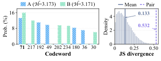
We examine 20,000 ESCI-US item pairs with the same first-level hard code and teacher-entropy decile. Their mean Jensen–Shannon (JS) divergence is 0.1330 nats, with a 95th percentile of 0.3088 (Figure 6). The illustrated pair is selected for high divergence: both items are assigned to $c_{71}$ and have similar entropies, 3.173 and 3.171 nats, yet their strongest alternatives are $c_{192}$ and $c_{217}$ . The JS divergence between their distributions is 0.5322 nats. This variation captures information beyond the hard code. Section 5.2 evaluates its contribution to retrieval performance.

C.2.2 Additional Retrieval Results

Table 9 extends the comparison in Section 5.2 to all five retrieval metrics, including Recall@5. Entries are means and sample standard deviations across three training seeds for each objective and locale.

Table 8 summarizes the control properties using the definitions in Table 3. Hard denotes preservation of the item’s assigned hard code. Shape describes how the target preserves the original teacher’s permutation-invariant probability profile: agg. denotes aggregate matching, coarse entropy-bin matching with a singleton fallback, near approximate shape matching, and exact preservation of the probability profile; unmatched denotes unrestricted teacher shuffling. Real denotes an unmodified distribution induced by an actual item. Averages and probability permutations are transformed targets. Pair denotes preservation of the original item–teacher correspondence. Checkmarks and crosses indicate whether a binary property is preserved. Dashes denote inapplicable properties. Base-FT has no auxiliary teacher. For RBD + future hard SID, the properties refer to the hard future targets, while current-level supervision remains unchanged. For Codebook-only ( $H=4$ ), targets are constructed from the stored code and frozen codebook without item residuals or corpus residual statistics. The dash in Shape indicates that no residual-teacher probability profile is used or matched.

Table 8: Properties of the teacher-target controls. Hard, Shape, Real, and Pair follow the definitions in Table 3. Properties are shared across all three locales.

Teacher objective	Hard	Shape	Real	Pair
Base-FT	$\checkmark$	–	–	–
Shuffled ResTD	×	unmatched	$\checkmark$	×
RBD + future hard SID	$\checkmark$	–	–	–
Codebook-only (H=4)	$\checkmark$	–	×	×
Code-conditioned mean	$\checkmark$	agg.	×	×
Same-code + entropy-bin shuffle	$\checkmark$	coarse	$\checkmark$	×
Non-target permutation	$\checkmark$	exact	×	×
Shape-matched teacher swap	$\checkmark$	near	$\checkmark$	×
ResTD (H=4)	$\checkmark$	exact	$\checkmark$	$\checkmark$

Table 9: Complete teacher-target comparison on ESCI (%), including Recall@5. Entries are mean ± standard deviation across three training seeds. Teacher properties and full control names are given in Table 8. Bold marks the highest means.

Teacher objective	R@5	R@10	R@100	N@10	N@100
ESCI-US
Base-FT	7.62_± 0.03	12.82_± 0.16	37.60_± 0.13	11.25_± 0.11	18.92_± 0.15
Shuffled ResTD	7.65_± 0.14	12.86_± 0.05	37.68_± 0.11	11.22_± 0.12	18.95_± 0.03
RBD + future hard SID	8.51_± 0.16	13.56_± 0.09	38.68_± 0.07	12.18_± 0.08	19.93_± 0.13
Codebook-only (H=4)	8.38_± 0.10	13.48_± 0.11	38.55_± 0.06	12.05_± 0.14	19.81_± 0.03
Code-conditioned mean	8.91_± 0.12	13.90_± 0.08	39.03_± 0.15	12.50_± 0.10	20.27_± 0.16
Entropy-bin shuffle	8.88_± 0.04	13.82_± 0.07	38.96_± 0.10	12.44_± 0.06	20.22_± 0.11
Non-target permutation	8.73_± 0.12	13.76_± 0.10	38.86_± 0.16	12.36_± 0.15	20.12_± 0.09
Shape-matched swap	9.13_± 0.17	14.16_± 0.10	39.36_± 0.07	12.79_± 0.03	20.58_± 0.11
ResTD (H=4)	9.28_± 0.09	14.34_± 0.04	39.58_± 0.11	12.99_± 0.07	20.79_± 0.05
ESCI-ES
Base-FT	6.10_± 0.10	10.55_± 0.15	34.22_± 0.11	12.53_± 0.12	19.95_± 0.09
Shuffled ResTD	6.08_± 0.11	10.51_± 0.06	34.10_± 0.04	12.60_± 0.14	19.92_± 0.03
RBD + future hard SID	6.47_± 0.09	11.16_± 0.04	34.81_± 0.05	13.40_± 0.10	20.71_± 0.15
Codebook-only (H=4)	6.35_± 0.09	10.98_± 0.11	34.65_± 0.13	13.22_± 0.12	20.51_± 0.08
Code-conditioned mean	6.62_± 0.15	11.39_± 0.06	35.00_± 0.08	13.66_± 0.03	20.97_± 0.13
Entropy-bin shuffle	6.50_± 0.14	11.29_± 0.11	34.89_± 0.07	13.60_± 0.09	20.91_± 0.12
Non-target permutation	6.55_± 0.03	11.29_± 0.04	34.93_± 0.15	13.54_± 0.12	20.84_± 0.06
Shape-matched swap	6.76_± 0.08	11.61_± 0.11	35.23_± 0.03	14.00_± 0.05	21.31_± 0.07
ResTD (H=4)	6.86_± 0.03	11.76_± 0.04	35.38_± 0.13	14.22_± 0.07	21.54_± 0.12
ESCI-JP
Base-FT	6.08_± 0.13	9.85_± 0.03	30.98_± 0.07	11.90_± 0.17	18.55_± 0.08
Shuffled ResTD	6.10_± 0.04	9.89_± 0.06	31.02_± 0.12	11.88_± 0.13	18.59_± 0.07
RBD + future hard SID	6.78_± 0.12	10.81_± 0.03	31.96_± 0.11	13.12_± 0.07	19.72_± 0.16
Codebook-only (H=4)	6.62_± 0.10	10.63_± 0.14	31.76_± 0.09	12.95_± 0.15	19.51_± 0.16
Code-conditioned mean	7.11_± 0.08	11.09_± 0.13	32.24_± 0.10	13.47_± 0.05	20.05_± 0.15
Entropy-bin shuffle	7.09_± 0.08	11.03_± 0.04	32.17_± 0.13	13.44_± 0.10	20.03_± 0.05
Non-target permutation	6.96_± 0.17	10.96_± 0.04	32.11_± 0.05	13.31_± 0.10	19.89_± 0.12
Shape-matched swap	7.41_± 0.12	11.41_± 0.04	32.61_± 0.07	13.90_± 0.09	20.49_± 0.17
ResTD (H=4)	7.61_± 0.07	11.63_± 0.17	32.86_± 0.09	14.18_± 0.08	20.79_± 0.05

C.2.3 Control Construction

Let $\mathcal{D}_{\mathrm{train}}$ be the set of distinct training items. For an item $d$ and target level $\ell$ , write $y_{\ell}(d)$ for its stored code and $\widetilde{{\mathcal{Q}}}_{\ell}(d)$ for its collision-corrected teacher. Each control defines a teacher for a valid item–level pair $(d,\ell)$ before training. This teacher is held fixed and used for every valid state–horizon pair $(t,s)$ satisfying $t+s=\ell$ . The transformation therefore applies to both current ( $s=0$ ) and future ( $s>0$ ) targets. Table 10 summarizes these constructions. RBD + future hard SID is the exception: it preserves current-level RBD and replaces only $s>0$ targets with one-hot identifiers.

Non-target permutation.

For each $(d,\ell)$ , a fixed random permutation reassigns the probabilities of the $K_{\ell}-1$ non-target codewords while leaving $\widetilde{{\mathcal{Q}}}_{\ell}(y_{\ell}(d)\mid d)$ unchanged. The complete probability multiset is preserved, including entropy, assigned-code confidence, and the largest alternative probability. Only the association between non-target codewords and their probabilities changes. This permutation is held fixed wherever the item–level target is used.

Codebook-only targets.

For each target level $\ell$ , we construct a distribution from the distances between the stored codeword and all codewords in the frozen codebook. Items sharing a stored code at the same level receive identical targets. This uses no item residuals or corpus residual statistics.

Code-conditioned mean.

For each target level $\ell$ and stored code $c$ , define

\overline{{\mathcal{Q}}}_{\ell,c}=\frac{1}{|\mathcal{D}_{\ell,c}|}\sum_{d\in\mathcal{D}_{\ell,c}}\widetilde{{\mathcal{Q}}}_{\ell}(d),\qquad\mathcal{D}_{\ell,c}=\{d\in\mathcal{D}_{\mathrm{train}}:y_{\ell}(d)=c\}.

(25)

The mean is computed before training for each level and code, with equal weight for every distinct item. Assigning this distribution to all items in $\mathcal{D}_{\ell,c}$ preserves code-conditioned population preferences while removing variation among items with the same code.

Same-code + entropy-bin shuffle.

At each target level, we stably sort the corrected training teachers by $(\mathcal{H}(\widetilde{{\mathcal{Q}}}_{\ell}(d)),\mathrm{item\ ID})$ and partition them into ten equal-frequency entropy bins. Within each group sharing the same level, stored hard code, and entropy bin, items are ordered by ID and their teachers are cyclically permuted. Groups of size at least two therefore receive a teacher from another item. For a singleton group, the donor is the other training item with the closest teacher entropy at the same level and stored code; ties are resolved by item ID. This fallback may cross an entropy-bin boundary while preserving the hard code. Assignments remain fixed throughout training. The 100% replacement rate includes these singleton assignments and therefore measures replacement by another item’s teacher, not exact entropy-bin agreement.

Shape-matched teacher swap.

For a corrected teacher $\widetilde{{\mathcal{Q}}}$ with stored code $c$ , define

v_{c}(\widetilde{{\mathcal{Q}}})=\left[\widetilde{{\mathcal{Q}}}(c),\,\operatorname{sort}_{\downarrow}\{\widetilde{{\mathcal{Q}}}(k):k\neq c\}\right].

(26)

Candidate donors are other training items at the same target level and stored hard code. We use the $L_{1}$ distance between shape vectors for greedy one-to-one nearest matching without replacement, forming disjoint item pairs. Distance ties are resolved deterministically by item ID. The two items in each pair exchange their complete, unmodified corrected teachers, so no donor is reused. In a group of odd size, the final unpaired item retains its own teacher and is counted as unswapped. The pairing is constructed once before training and shared across optimization steps and training seeds 42, 2027, and 2028. The replacement rate of 99.76–99.91% excludes items that retain their own teacher.

The replacement rates in Table 10 count transformation applications for synthetic, aggregate, and hard targets, including those that leave the target distribution unchanged. For real-item controls, they count assignments to another item’s teacher. Each rate uses all valid item–level targets in the indicated scope. This ensures consistent accounting across the different control constructions.

Table 10: Construction of teacher controls across current and future targets. Assignments remain fixed during training; replacement rates are measured over valid item–level targets within each scope.

Control	Scope	Matching unit	Fixed	Target replacement
Non-target permutation	Current + future	Item × level	$\checkmark$	100% synthetic
Code-conditioned mean	Current + future	Level × hard code	$\checkmark$	100% aggregate
Entropy-bin shuffle	Current + future	Level × code × entropy decile^*	$\checkmark$	100% real-item
Shape-matched swap	Current + future	Level × code	$\checkmark$	99.76–99.91% real-item
Future hard SID	Future only	–	$\checkmark$	100% hard target

^*Singleton groups retain the level and hard code but may use a donor from another entropy bin.

C.2.4 Matching Quality

For a donor–recipient pair $(d^{\prime},d)$ at level $\ell$ , define ${\mathcal{Q}}^{\prime}=\widetilde{{\mathcal{Q}}}_{\ell}(d^{\prime})$ , ${\mathcal{Q}}=\widetilde{{\mathcal{Q}}}_{\ell}(d)$ , and $c=y_{\ell}(d^{\prime})=y_{\ell}(d)$ . We quantify entropy, assigned-code probability, and shape differences as

	$\displaystyle\|\Delta\mathcal{H}\|$	$\displaystyle=\|\mathcal{H}({\mathcal{Q}}^{\prime})-\mathcal{H}({\mathcal{Q}})\|,$	$\displaystyle\mathcal{H}({\mathcal{Q}})$	$\displaystyle=-\sum_{k}{\mathcal{Q}}(k)\log{\mathcal{Q}}(k),$
	$\displaystyle\|\Delta q_{y}\|$	$\displaystyle=\|{\mathcal{Q}}^{\prime}(c)-{\mathcal{Q}}(c)\|,$	$\displaystyle D_{\mathrm{shape}}$	$\displaystyle=\\|v_{c}({\mathcal{Q}}^{\prime})-v_{c}({\mathcal{Q}})\\|_{1}.$		(27)

Entropy is measured in nats. Matching statistics are computed over donor–recipient pairs with distinct item identities. Coverage is the fraction of valid training item–level targets assigned another item’s teacher, even when the donor and recipient have identical probability vectors.

Table 11: Matching quality for shape-matched teacher swap. Mismatch summaries are medians except P90 (90th percentile), computed over pairs with different item identities. Coverage uses all valid training item–level targets. Entropy uses nats; probability differences and Shape L₁ are unitless.

	Median $\|\Delta\mathcal{H}\|$	Median $\|\Delta q_{y}\|$	Shape L₁		Swap coverage (%)
Locale	(nats)		Median	P90
US	0.008	0.0018	0.018	0.046	99.91
ES	0.012	0.0027	0.026	0.064	99.76
JP	0.010	0.0023	0.023	0.057	99.81

Median entropy mismatch is 0.008–0.012 nats, and median assigned-code probability mismatch is 0.0018–0.0027, corresponding to 0.18–0.27 percentage points. Median Shape $L_{1}$ is 0.018–0.026, with P90 values of 0.046–0.064. Different-item coverage is 99.76–99.91%. The label near in Table 3 refers to this approximate shape matching. Similar profiles can have different codeword probabilities.

C.3 Output-Space Supervision

C.3.1 Full-Distribution Output Distillation

Full-output KD applies the collision-corrected current-level teacher $\widetilde{{\mathcal{Q}}}_{t}$ directly to the retriever’s SID output distribution. Let $z_{t,j}$ denote its output logit for codeword $j$ at level $t$ . We define

{\mathcal{P}}_{t}^{\mathrm{out}}(j\mid q,y_{<t})=\frac{\exp z_{t,j}}{\sum_{k=1}^{K_{t}}\exp z_{t,k}},\qquad\mathcal{L}_{\mathrm{FullOut}}=\frac{\sum_{t=1}^{L}m_{t}\,\mathrm{KL}(\widetilde{{\mathcal{Q}}}_{t}\|{\mathcal{P}}_{t}^{\mathrm{out}})}{\sum_{t=1}^{L}m_{t}}.

(28)

Here $m_{t}$ selects valid SID positions. The full $K_{t}=256$ -way teacher retains the probabilities of the assigned code and all alternatives. Supervision targets the current SID position.

Full-output KD and RBD ( $H=1$ ) use the same teacher and train for 1,200 updates with learning rate $10^{-5}$ and 120-step warmup. Initial parameters and minibatch order are matched within seeds 42, 2027, and 2028. Both retain the original retrieval objective and use the auxiliary schedule in Equation 15, with $\lambda_{\max}=0.1$ and a cap of 5% of the SID loss, treated as constant during backpropagation. Full-output KD supervises SID output probabilities. RBD supervises a projected decoder state evaluated against the frozen codebook. Gradient norms depend on the supervision parameterization.

Table 12: Full-output KD on ESCI (%). Values are mean ± sample standard deviation across seeds 42, 2027, and 2028. All five retrieval metrics are reported.

Locale	R@5	R@10	R@100	N@10	N@100
US	7.95_± 0.08	13.15_± 0.07	38.10_± 0.13	11.69_± 0.10	19.35_± 0.09
ES	6.27_± 0.07	10.80_± 0.05	34.40_± 0.11	12.91_± 0.06	20.20_± 0.14
JP	6.35_± 0.08	10.22_± 0.09	31.39_± 0.08	12.39_± 0.11	18.99_± 0.12

Full-output KD improves over Base-FT by 0.50, 0.18, and 0.41 percentage points in Recall@100 on US, ES, and JP, respectively. Current-level RBD adds 0.10, 0.06, and 0.09 points over Full-output KD, with NDCG@10 gains of 0.09, 0.07, and 0.11 points. Both objectives improve retrieval, with higher mean scores for current-level codebook distillation.

C.3.2 Non-Target Output Alignment

This control aligns the retriever’s output probabilities over alternative codes. At each valid position, we remove the assigned code from the teacher and student distributions and renormalize the remaining mass. Writing these conditional distributions as $\overline{{\mathcal{Q}}}_{t}$ and $\overline{{\mathcal{P}}}_{t}$ , the auxiliary loss is

\mathcal{L}_{\mathrm{out}}=\frac{1}{|\mathcal{T}|}\sum_{t\in\mathcal{T}}\mathrm{KL}(\overline{{\mathcal{Q}}}_{t}\|\overline{{\mathcal{P}}}_{t}),

(29)

where $\mathcal{T}$ contains valid positions with positive alternative teacher mass. The original gold-SID objective is unchanged. The auxiliary term has coefficient 0.02 and is capped at 1% of the SID loss. The cap is treated as constant during backpropagation. Table 2 reports the retrieval results.

C.4 Probing Current and Future Codebook Preferences

C.4.1 Current-Target Diagnostic

For the current-level diagnostic in Figure 7, we freeze one pair of trained Base-FT and RBD models per locale and fit a new projection for each model. The projection is shared across all four SID levels and consists of a linear map from $d_{h}$ to $d_{h}$ , GELU, LayerNorm, and a linear map to residual dimension $D$ . It contains $d_{h}^{2}+d_{h}D+3d_{h}+D$ trainable parameters. The probes are fitted for ten epochs with AdamW, learning rate $10^{-3}$ , and weight decay 0.01. Probe initialization and minibatch order use seed 4242 for both retrievers within each locale. We evaluate the epoch-10 probes.

The fitting sets contain 991, 267, and 319 queries for US, ES, and JP, respectively. Each evaluation set contains 256 disjoint queries. Targets are collision-corrected teachers with floor 0.1 and margin 0.001. We compute paired query-bootstrap intervals for each fixed pair of trained retrievers.

Figure 7 reports relative KL reductions of 0.06–1.84% for current-level RBD versus Base-FT across the three locales and four SID levels. This diagnostic measures recovery of current-level teacher preferences from the frozen decoder representations.

Figure 7: Relative held-out probe KL reduction for current-level RBD (

H=1

) versus Base-FT across four SID levels. Error bars show paired 95% query-bootstrap intervals conditional on one pair of trained Base-FT and RBD models for each locale.

C.4.2 Future-Target Comparison

We compare frozen RBD ( $H=1$ ) and ResTD ( $H=4$ ) models. For each retriever, we fit a separate probe at each offset $s=j-t\in\{0,1,2,3\}$ . All valid state–target pairs $(t,j)$ with the same offset share that probe. Each probe has the architecture

\mathrm{Linear}(d_{h},d_{h})\ \to\ \mathrm{GELU}\ \to\ \mathrm{LayerNorm}\ \to\ \mathrm{Linear}(d_{h},D).

(30)

With $d_{h}=768$ and $D=32$ , each probe contains $d_{h}^{2}+d_{h}D+3d_{h}+D=616{,}736$ trainable parameters. The probe capacity and fitting procedure are identical across retriever conditions.

For each locale, 1,024 queries are used to fit the probes and 512 disjoint queries are reserved for evaluation. These splits are fixed across conditions and retriever seeds. Probes are trained for ten epochs with AdamW, learning rate $10^{-3}$ , weight decay 0.01, and batch size 64. We evaluate the epoch-10 probes. Probe initialization and minibatch order use seed 4242 throughout. The three replicates correspond to retrievers trained with seeds 42, 2027, and 2028, with probe initialization and query splits held fixed.

The target is the collision-corrected teacher $\widetilde{{\mathcal{Q}}}_{j}$ used in retriever training, with floor 0.1 and margin 0.001. We report held-out forward KL from the complete corrected teacher, including the assigned-code mass, to the probe’s codebook distribution.

The two probing studies use separate query splits. Model comparisons use the common split within each study. For a four-level SID, offset $s$ has $4-s$ valid state–target pairs. Although pairs with the same offset share probe parameters, held-out KL is evaluated separately for each valid pair $(t,j)$ . Figure 4 reports the relative reduction $100(1-\mathrm{KL}_{H=4}(t,j)/\mathrm{KL}_{H=1}(t,j))$ from current-level RBD to ResTD. Diagonal cells ( $j=t$ ) correspond to current targets; cells with $j>t$ correspond to future targets.

C.5 Multi-Positive Teacher Disagreement

C.5.1 Item-Conditioned Teacher Targets

Several relevant items can induce different teachers for the same query. Let $\mathcal{D}^{+}(q,p)$ contain the relevant items whose SIDs share prefix $p$ before position $t$ . They share the teacher-forced decoding context, but may induce different codebook distributions ${\mathcal{Q}}_{t}(d)$ . Under uniform sampling within this set, write $\overline{{\mathcal{Q}}}_{t}=\mathbb{E}_{d}{\mathcal{Q}}_{t}(d)$ . For any common student distribution ${\mathcal{P}}_{t}$ , the forward-KL decomposition is

\mathbb{E}_{d}\,\mathrm{KL}({\mathcal{Q}}_{t}(d)\|{\mathcal{P}}_{t})=\mathbb{E}_{d}\,\mathrm{KL}({\mathcal{Q}}_{t}(d)\|\overline{{\mathcal{Q}}}_{t})+\mathrm{KL}(\overline{{\mathcal{Q}}}_{t}\|{\mathcal{P}}_{t}).

(31)

For a shared decoding context, an unrestricted student minimizes the expected forward-KL objective at the mean teacher distribution $\overline{{\mathcal{Q}}}_{t}$ . The first term is the generalized Jensen–Shannon divergence among the item-conditioned teachers and is constant with respect to the student. With nonuniform item sampling, the identity holds for the corresponding weighted mean.

To obtain Equation 31, expand the KL terms and collect the coefficient of $\log(\overline{{\mathcal{Q}}}_{t}/{\mathcal{P}}_{t})$ . Since $\mathbb{E}_{d}{\mathcal{Q}}_{t}(d)=\overline{{\mathcal{Q}}}_{t}$ , this coefficient is $\overline{{\mathcal{Q}}}_{t}$ . The remaining term equals $H(\overline{{\mathcal{Q}}}_{t})-\mathbb{E}_{d}H({\mathcal{Q}}_{t}(d))$ , the generalized JS divergence. This decomposition concerns teachers at a common decoding context. The tables below report mean pairwise JS, which is bounded by $\log 2$ . Generalized JS over several teachers need not satisfy that bound.

Table 13: ResTD (H=4) gains by first-level teacher disagreement among multi-positive queries. JS is mean pairwise Jensen–Shannon divergence in nats; Pos./query is the mean number of distinct positive items. Metric differences are in percentage points, averaged across three runs.

ESCI-US: ResTD vs. Base-FT
Group	$n$	JS	Pos./query	$\Delta$ R@5	$\Delta$ R@10	$\Delta$ R@100	$\Delta$ N@10	$\Delta$ N@100
Low	1,550	0.236	3.92	+1.46	+1.34	+1.74	+1.39	+1.47
Medium	1,550	0.394	4.48	+1.82	+1.62	+2.17	+1.95	+2.14
High	1,549	0.538	5.13	+2.24	+2.04	+2.59	+2.43	+2.55
ESCI-US: ResTD vs. RBD (H=1)
Low	1,550	0.236	3.92	+1.04	+0.93	+1.17	+0.85	+1.04
Medium	1,550	0.394	4.48	+1.38	+1.20	+1.50	+1.34	+1.54
High	1,549	0.538	5.13	+1.70	+1.51	+1.87	+1.82	+1.88
ESCI-ES: ResTD vs. Base-FT
Low	450	0.432	3.79	+0.58	+0.86	+0.79	+1.34	+1.35
Medium	449	0.580	4.71	+0.96	+1.43	+1.33	+2.08	+1.81
High	449	0.658	5.16	+0.81	+1.43	+1.43	+1.75	+1.72
ESCI-ES: ResTD vs. RBD (H=1)
Low	450	0.432	3.79	+0.46	+0.59	+0.51	+0.95	+0.97
Medium	449	0.580	4.71	+0.72	+1.08	+1.12	+1.56	+1.43
High	449	0.658	5.16	+0.65	+1.13	+1.17	+1.30	+1.41
ESCI-JP: ResTD vs. Base-FT
Low	512	0.409	3.93	+0.95	+1.04	+1.20	+1.40	+1.39
Medium	511	0.570	4.77	+1.51	+2.21	+2.15	+2.72	+2.82
High	511	0.652	5.13	+2.47	+2.55	+2.76	+3.37	+3.09
ESCI-JP: ResTD vs. RBD (H=1)
Low	512	0.409	3.93	+0.71	+0.76	+0.83	+0.83	+1.00
Medium	511	0.570	4.77	+1.21	+1.60	+1.59	+2.01	+2.17
High	511	0.652	5.13	+1.95	+1.98	+2.08	+2.64	+2.35

C.5.2 Teacher Disagreement Statistics

We compute disagreement from the first-level teachers used in training, including the SID-consistency correction. For each query with at least two distinct E/S/C-positive items, we average the pairwise JS divergence between its positive-item teachers. Dataset means assign equal weight to each query.

US, ES, and JP contain 4,649, 1,348, and 1,534 multi-positive queries out of 6,014, 1,656, and 1,883 test queries, respectively. Their mean JS divergences are 0.389, 0.557, and 0.543 nats. The remaining 1,365, 308, and 349 queries have a single positive item, respectively. Within the multi-positive sets, 5 US, 12 ES, and 1 JP queries contain distinct positive items with identical complete SIDs. Disagreement uses distinct items, and retrieval metrics use distinct SIDs.

C.5.3 Retrieval Gains by Teacher Disagreement

Within each locale, we divide multi-positive queries into low, medium, and high first-level disagreement groups of approximately equal size. For each query, we compare ResTD ( $H=4$ ) with Base-FT and current-level RBD ( $H=1$ ), averaging the paired metric differences across three runs. Differences are reported in percentage points, and each query receives equal weight within its group. Table 13 reports query counts, mean pairwise JS divergence in nats, mean positive-item counts, and the five retrieval gains. The group sizes differ by at most one query. Figure 4 plots the group means for Recall@100 and NDCG@10. The stratified comparisons and adjusted regressions examine query-level associations between teacher disagreement and retrieval gains.

Table 14: Teacher disagreement and ResTD gains among multi-positive queries. Raw

\rho

is the Spearman correlation. Adjusted coefficients are changes in gain (pp) per 0.1-nat increase in JS, controlling for

\log(\textnormal{1}+\text{positive items})

and the corresponding score of the common model before fine-tuning (Equation 32). Brackets contain 95% HC3 confidence intervals.

		Recall@100		NDCG@10
Locale	Compared with	Raw $\rho$	Adjusted [95% CI]	Raw $\rho$	Adjusted [95% CI]
US	Base-FT	+0.080	+0.16 [+0.04, +0.28]	+0.090	+0.19 [+0.08, +0.30]
US	RBD (H=1)	+0.081	+0.10 [+0.01, +0.19]	+0.105	+0.17 [+0.08, +0.25]
ES	Base-FT	+0.060	+0.16 [−0.15, +0.48]	+0.051	+0.12 [−0.20, +0.43]
ES	RBD (H=1)	+0.073	+0.16 [−0.09, +0.40]	+0.055	+0.06 [−0.19, +0.31]
JP	Base-FT	+0.114	+0.55 [+0.26, +0.83]	+0.148	+0.72 [+0.42, +1.02]
JP	RBD (H=1)	+0.123	+0.43 [+0.20, +0.65]	+0.168	+0.62 [+0.39, +0.85]

C.5.4 Adjusted Associations

Let $J_{q}$ denote first-level teacher disagreement and $m_{q}$ the number of distinct positive items. Initial query difficulty is measured using our reproduced CaLIR model $\theta_{\mathrm{init}}$ , before fine-tuning with Base-FT, RBD, or ResTD. For the metric $M$ under analysis, define

s_{q}^{(M)}=M(q;\theta_{\mathrm{init}}),\qquad M\in\{\mathrm{Recall}@100,\mathrm{NDCG}@10\}.

(32)

Initial and final scores use the same decoder and SID-level evaluation protocol (Appendix A.3). The initial score is fixed for each query and metric across all conditions and seeds. Both initial and final scores are expressed on the $[0,100]$ scale. The paired gain over baseline $b\in\{\text{Base-FT},H=1\}$ is

\overline{\Delta}_{q,b}^{(M)}=\frac{1}{3}\sum_{r=1}^{3}\left[M(q;\theta_{H4,r})-M(q;\theta_{b,r})\right],

(33)

where $r$ indexes the three paired runs. For each locale, metric, and baseline, we fit

\overline{\Delta}_{q,b}^{(M)}=\alpha+\beta\frac{J_{q}}{0.1}+\gamma\log(1+m_{q})+\eta s_{q}^{(M)}+\varepsilon_{q},

(34)

where $\overline{\Delta}_{q,b}^{(M)}$ is the mean gain of ResTD over baseline $b$ , in percentage points across the three paired runs. Each multi-positive query contributes one observation. The coefficient $\beta$ measures the adjusted change in gain per 0.1-nat increase in JS. Table 14 reports the raw rank correlations and coefficients with 95% HC3 heteroskedasticity-robust confidence intervals. The intervals quantify query-level uncertainty conditional on the fitted retrievers.

For each 0.1-nat increase in JS, the adjusted NDCG@10 gain over $H=1$ is 0.17 points (95% CI: 0.08–0.25) on US, 0.06 points ( $-0.19$ –0.31) on ES, and 0.62 points (0.39–0.85) on JP.

C.6 Collision-Aware Teacher Analysis

C.6.1 Frequency and Magnitude of Teacher–SID Conflicts

For each locale and quantization level, Table 15 reports two rates over all items. SID edited is the fraction whose stored code differs from the original nearest-code assignment after collision resolution. Raw conflict is the fraction whose uncorrected teacher does not rank the stored code highest, with residuals reconstructed along the final SID path (Section 4.3).

For each conflicting target, we compute the minimum one-hot mixing weight needed to satisfy the margin constraint in Equation 12 with $\delta=0.001$ for the corrected teacher defined in Equation 13:

\epsilon^{\star}=\left[\frac{q_{\max}-q_{y}+\delta}{1-q_{y}+q_{\max}}\right]_{0}^{1},

(35)

where $q_{y}$ is the raw probability of the stored code and $q_{\max}$ is the largest probability among competing codes. The applied mixing weight is $\max\{\epsilon,\epsilon^{\star}\}$ , with floor $\epsilon$ . The $\epsilon^{\star}$ summaries in Table 15 are conditional on a raw conflict.

Table 15: Frequency and magnitude of teacher–SID conflicts across ESCI locales and quantization levels. Rates use all items;

\epsilon^{\star}

statistics are computed only over conflicting targets.

				Among conflicting targets
Locale	Level	SID edited (%)	Raw conflict (%)	Mean $\epsilon^{\star}$	Median	P90	P95	$\epsilon^{\star}<\textnormal{0.1}$ (%)
US	1	0.2	0.2	0.031	0.024	0.066	0.082	97.1
US	2	0.6	0.9	0.039	0.030	0.081	0.101	94.8
US	3	2.1	2.6	0.055	0.043	0.112	0.137	86.4
US	4	7.8	10.1	0.083	0.071	0.157	0.201	67.5
ES	1	0.3	0.3	0.034	0.026	0.070	0.088	96.3
ES	2	0.8	1.2	0.042	0.033	0.087	0.109	92.7
ES	3	2.7	3.7	0.059	0.047	0.120	0.149	83.6
ES	4	9.4	12.9	0.088	0.075	0.166	0.214	63.1
JP	1	0.2	0.2	0.033	0.025	0.069	0.085	96.8
JP	2	0.7	0.8	0.041	0.032	0.085	0.106	93.4
JP	3	2.5	3.2	0.058	0.046	0.118	0.145	84.2
JP	4	8.8	11.7	0.086	0.073	0.162	0.207	65.4

Conflicts become more frequent at greater quantization depth. At the first level, conflict rates equal the rates of direct SID modification: 0.2% on US, 0.3% on ES, and 0.2% on JP. At this level, the residual has not been affected by earlier collision-resolved assignments. At the fourth level, conflict rates reach 10.1%, 12.9%, and 11.7%, exceeding the direct edit rates of 7.8%, 9.4%, and 8.8%, respectively. Changes to earlier codes alter the residuals used by subsequent teachers, allowing conflicts even at positions whose codes were not modified. Most conflicts require only a small correction: 96.3–97.1% have $\epsilon^{\star}<0.1$ at the first level. The required mixing weight increases at later levels, but 63.1–67.5% of fourth-level conflicts still fall below 0.1.

Table 16: Retrieval performance (%) under collision-aware teacher correction for ResTD (H=4) on ESCI. Values are mean ± standard deviation across three paired training seeds in each locale.

		ESCI-US		ESCI-ES		ESCI-JP
Correction strategy	Floor $\epsilon$	R@100	N@10	R@100	N@10	R@100	N@10
None (raw teacher)	–	39.20_± 0.13	12.66_± 0.08	35.04_± 0.12	13.79_± 0.10	32.43_± 0.14	13.68_± 0.11
Adaptive only	0	39.53_± 0.13	12.95_± 0.08	35.34_± 0.12	14.17_± 0.09	32.81_± 0.13	14.12_± 0.11
Adaptive + floor	0.05	39.54_± 0.12	12.95_± 0.08	35.36_± 0.12	14.21_± 0.09	32.85_± 0.13	14.16_± 0.10
Adaptive + floor	0.10	39.58_± 0.11	12.99_± 0.07	35.38_± 0.13	14.22_± 0.07	32.86_± 0.09	14.18_± 0.08
Adaptive + floor	0.20	39.51_± 0.13	12.92_± 0.09	35.31_± 0.12	14.14_± 0.10	32.77_± 0.14	14.07_± 0.11

C.6.2 Retrieval Sensitivity to Collision Correction

Table 16 varies only teacher correction in ResTD ( $H=4$ ), holding the index, training, evaluation, and three paired seeds fixed. None (raw teacher) uses ${\mathcal{Q}}$ without correction; Adaptive only applies $\epsilon^{\star}$ with zero floor. The remaining conditions use $\max\{\epsilon,\epsilon^{\star}\}$ with floors 0.05, 0.10, and 0.20. All corrected conditions use margin $\delta=0.001$ ; the main experiments use $\epsilon=0.10$ .

Relative to the raw teacher, correction with $\epsilon=0.10$ improves Recall@100 by 0.38, 0.34, and 0.43 percentage points on US, ES, and JP, respectively; the corresponding NDCG@10 gains are 0.33, 0.43, and 0.50 points. Adaptive-only correction recovers most of these gains; mean scores vary by only 0.04–0.06 points across floors 0, 0.05, and 0.10 for each locale–metric pair. Raising the floor to 0.20 reduces scores by 0.07–0.11 points relative to $\epsilon=0.10$ . Stronger one-hot mixing shifts probability mass from alternative codewords to the stored code.

C.7 Hyperparameter Sensitivity

We vary $\lambda_{\max}\in\{0.025,0.05,0.1,0.15,0.2\}$ , $\tau_{T}=\tau_{S}\in\{0.05,0.1,0.2,0.3,0.5\}$ , and $\rho\in\{0.3,0.5,0.7,0.9,1.0\}$ one at a time, keeping the remaining settings fixed. All locales use the defaults in Section 5.1. Figure 8 reports Recall@10 and NDCG@10 for each locale. Appendix C.6.2 separately evaluates the collision-correction floor $\epsilon$ over three training seeds.

Auxiliary loss weight.

Increasing $\lambda_{\max}$ does not yield a monotonic improvement. Among the tested values, $0.05$ gives the highest Recall@10 on US and JP, while ES peaks at the default $0.1$ . On JP, the two metrics favor different weights, with NDCG@10 highest at $0.15$ . The coefficient in Equation 15 is also subject to the 5% SID-loss cap. Consequently, increasing $\lambda_{\max}$ need not produce a proportional increase in the effective auxiliary contribution.

Teacher and student temperature.

The preferred temperature varies across locales: both metrics peak at $0.3$ on US, $0.2$ on ES, and $0.05$ on JP within the tested grid. The effect is not monotonic, and the common default $0.2$ does not maximize every curve. Temperature changes the concentration of the codeword distributions and the gradient scale of the student objective (Equation 7). Since $\tau_{T}$ and $\tau_{S}$ are varied jointly, this sweep measures their combined effect and does not isolate teacher softness from student optimization.

Horizon discount.

Larger $\rho$ assigns more relative weight to distant targets in Equation 10. The largest plotted scores occur at $\rho=0.9$ on US, $0.5$ on ES, and $0.3$ on JP. For $H=L=4$ with all positions valid, the total weight at offset $s$ is proportional to $(4-s)\rho^{s}$ . Thus, $\rho=1$ gives offset weights in the ratio $4{:}3{:}2{:}1$ , because fewer state–target pairs are available at longer offsets. All tested discounts retain supervision at all four offsets, so this comparison concerns the allocation of trajectory supervision with its horizon range fixed.

The shared defaults specify a common configuration across locales. These sweeps describe sensitivity to individual parameters with the other settings fixed; interactions among parameters are not evaluated.

Figure 8: Hyperparameter sensitivity on ESCI-US (top), ESCI-ES (middle), and ESCI-JP (bottom). Rows show Recall@10 and NDCG@10; columns vary

\lambda_{\max}

\tau_{T}=\tau_{S}

, and

\rho

one at a time. Dashed lines and filled markers indicate the shared defaults. Each panel uses its own vertical scale.

Appendix D Qualitative Case Study

Figure 9 presents six selected ESCI queries across US, ES, and JP, covering Exact (E), Substitute (S), and Complement (C) judgments. Each panel pairs a judged target with CaLIR’s top-ranked product. U denotes an unjudged product, for which the dataset provides no relevance label. Both models use the same SID index and a beam width of 100. Rank@100 is the target SID’s position among the top 100 results, and NDCG@100 measures query-level ranking quality on the $[0,1]$ scale. The SID rows show the complete target sequence retrieved by each model. The exact-match cases involve specific compatibility and product-attribute requirements. In panel (c), ResTD promotes the Huawei P30 Lite case from rank 4 to 1; CaLIR places a case for the Mate 20 first. In panel (e), the query specifies both the Zojirushi brand and a gasket-free bottle design, and the exact-match target rises from rank 25 to 2. These examples require distinguishing products within the same category: phone-model compatibility determines which case fits, while the bottle query combines a brand preference with a design requirement, both of which must be met for a retrieved product to satisfy the query in full.

ResTD also promotes judged substitutes and complements. The substitute brake controller in panel (a) rises from rank 2 to 1, and the ghd straightener in panel (d) advances from rank 5 to 3 for the Dyson query. Among complementary products, the TV stand in panel (b) moves from rank 10 to 1, and the camera lens in panel (f) enters the top ten at rank 6, up from rank 13. The relevance judgments in these panels extend beyond exact product matches to alternatives and accessories associated with the query. Both models retrieve the complete target SID in all six cases, so the observed differences concern the ranking of targets already present in the retrieved lists. NDCG@100 also increases for every query. The gain depends on the full ranking: the bottle target moves from rank 25 to 2 while NDCG@100 rises from 0.291 to 0.354; the phone case moves from rank 4 to 1 while NDCG@100 rises from 0.264 to 0.613. Target rank tracks one judged product, whereas NDCG@100 also reflects the positions and binary relevance of the other retrieved products within the top 100 results.

	$\displaystyle\|\Delta\mathcal{H}\|$	$\displaystyle=\|\mathcal{H}({\mathcal{Q}}^{\prime})-\mathcal{H}({\mathcal{Q}})\|,$	$\displaystyle\mathcal{H}({\mathcal{Q}})$	$\displaystyle=-\sum_{k}{\mathcal{Q}}(k)\log{\mathcal{Q}}(k),$
	$\displaystyle\|\Delta q_{y}\|$	$\displaystyle=\|{\mathcal{Q}}^{\prime}(c)-{\mathcal{Q}}(c)\|,$	$\displaystyle D_{\mathrm{shape}}$	$\displaystyle=\\|v_{c}({\mathcal{Q}}^{\prime})-v_{c}({\mathcal{Q}})\\|_{1}.$		(27)

Residual Trajectory Distillation for Generative Retrieval