DODGER: Safety-Guided Reinforcement Learning for Robot Navigation Among Dynamic Obstacles

We formulate navigation using a planar reduced-order model that captures translational motion in the forward and lateral directions of a body-fixed frame attached to the floating base, together with its heading motion. This representation provides a low-dimensional interface for constructing the CBF constraints independently of the full-order robot dynamics.

The state vector is given by $\bm{x}=[x,y,\phi,v_{f},v_{l}]^{\top}$, where $(x,y)$ denote the planar position of the floating base, $\phi$ denotes its heading angle, and $v_{f}$ and $v_{l}$ denote the forward and lateral velocities expressed in the body frame, respectively.

The reduced-order dynamics are given by

where the control input is $\bm{u}=[a_{f},a_{l},\omega]^{\top}$. Here, $a_{f}$ and $a_{l}$ denote the forward and lateral accelerations, respectively, and $\omega$ denotes the yaw angular velocity.

We consider $N_{\mathrm{obs}}$ detected dynamic obstacles, with the $j$-th obstacle state

where $(x_{\mathrm{obs}}^{j},y_{\mathrm{obs}}^{j})$, $\phi_{\mathrm{obs}}^{j}$, and $v_{\mathrm{obs}}^{j}$ denote its center, heading, and forward speed, respectively. Each obstacle is modeled with constant planar velocity during barrier evaluation, i.e., $\dot{\phi}_{\mathrm{obs}}^{j}=\dot{v}_{\mathrm{obs}}^{j}=0$ [14]. The superscript $j$ and explicit obstacle-state arguments are omitted below. All Lie derivatives are evaluated along the joint robot–obstacle dynamics.

Let $\bm{p}_{\mathrm{rob}}=[x,y]^{\top}$ and $\bm{p}_{\mathrm{obs}}=[x_{\mathrm{obs}},y_{\mathrm{obs}}]^{\top}$. The relative position and velocity are $\bm{p}_{\mathrm{rel}}=\bm{p}_{\mathrm{rob}}-\bm{p}_{\mathrm{obs}}$ and $\bm{v}_{\mathrm{rel}}=\bm{v}_{\mathrm{rob}}-\bm{v}_{\mathrm{obs}}$, where $\bm{v}_{\mathrm{rob}}=[\dot{x},\dot{y}]^{\top}$ and $\bm{v}_{\mathrm{obs}}=v_{\mathrm{obs}}[\cos\phi_{\mathrm{obs}},\sin\phi_{\mathrm{obs}}]^{\top}$. Following DPCBF [14], $\bm{v}_{\mathrm{rel}}$ is expressed in a line-of-sight (LoS) frame whose $\tilde{x}$-axis is aligned with $\bm{p}_{\mathrm{rel}}$, yielding $\tilde{\bm{v}}_{\mathrm{rel}}=[\tilde{v}_{\mathrm{rel},x},\tilde{v}_{\mathrm{rel},y}]^{\top}$. We approximate the planar footprints of the robot and obstacle by circles with radii $r_{\mathrm{rob}}$ and $r_{\mathrm{obs}}$, respectively, and define the combined safety radius $r=r_{\mathrm{rob}}+r_{\mathrm{obs}}$ and, for $\lVert\bm{p}_{\mathrm{rel}}\rVert>r$, the distance-dependent margin $d(\bm{x})=\sqrt{\lVert\bm{p}_{\mathrm{rel}}\rVert^{2}-r^{2}}$. The DPCBF parameters are $\lambda(\bm{x})=k_{\lambda}d(\bm{x})/\lVert\bm{v}_{\mathrm{rel}}\rVert$ and $\mu(\bm{x})=k_{\mu}d(\bm{x})$, where $k_{\lambda},k_{\mu}>0$. In implementation, $\lVert\bm{v}_{\mathrm{rel}}\rVert$ is lower-bounded by a small $\epsilon_{v}>0$ to avoid numerical singularity. The resulting DPCBF is

The parameters $\lambda(\bm{x})$ and $\mu(\bm{x})$ adapt the parabolic boundary to the relative robot–obstacle state: $\lambda(\bm{x})$ controls its curvature, while $\mu(\bm{x})$ shifts its vertex along the $\tilde{v}_{\mathrm{rel},x}$ axis. The boundary becomes less restrictive for more distant obstacles or smaller relative speeds, and more conservative as the obstacle approaches or the relative speed increases.

During training, DODGER computes a QP reference that penalizes deviations from the actor action $\bm{u}_{t}^{\pi}$ while incorporating DPCBF and input constraints. Its unrelaxed formulation is

Here, $\bm{u}_{t}=[a_{f,t},a_{l,t},\omega_{t}]^{\top}$ is the QP decision variable, and $h_{j}$ denotes the DPCBF in (4) constructed for the $j$-th detected obstacle. The superscripts $(\cdot)^{\mathrm{lb}}$ and $(\cdot)^{\mathrm{ub}}$ denote the lower and upper command bounds. During training, the unrelaxed QP was feasible in $99.6\%$ of solves; slack relaxation was used for the remaining $0.4\%$.

DODGER builds upon the Constraints as Terminations (CaT) principle [17], which maps soft constraint violations to termination probabilities used in return estimation. Rather than executing the CBF-filtered reference or terminating the rollout upon a constraint violation, DODGER continues the rollout with the actor action $\bm{u}^{\pi}_{t}$ and uses the resulting termination probability only when computing the learning target.

Let $\mathcal{I}_{c}$ and $\mathcal{I}_{r}$ denote the index sets of soft constraints and reward terms, respectively. We denote a constraint value by $c_{i_{c},t}=c_{i_{c}}(\bm{x}_{t},\bm{u}_{t}^{\pi})$, where positive values indicate violations, and define $c_{i_{c},t}^{+}=\max(0,c_{i_{c},t})$.

For the DPCBF constraint associated with the $j$-th obstacle, we define

For the input constraints, let

with corresponding lower and upper bounds $\bm{\xi}^{\mathrm{lb}}$ and $\bm{\xi}^{\mathrm{ub}}$. The violation of the $k$-th input constraint is defined as

Following CaT, each constraint $c_{i_{c},t}$ is associated with a maximum termination probability $p_{i_{c}}^{\max}$ that controls its enforcement strength. The termination probability is computed from the normalized constraint violations as

Larger violations increase $\delta_{t}$, reducing the positive return and bootstrapping contributions while the rollout continues with the actor action $\bm{u}_{t}^{\pi}$.

The normalization scale $c^{\max}_{i_{c}}$ is updated from the maximum constraint violation observed during each rollout using

where $\tau_{c}\in(0,1)$ is the exponential smoothing coefficient.

DODGER additionally uses the safety-filtered action as a reference through

which penalizes deviations of the actor action from the QP reference.

Directly applying the CaT factor $(1-\delta_{t})$ to signed rewards can undesirably weaken negative penalties, since multiplication by $(1-\delta_{t})$ reduces their magnitude. This is particularly relevant to navigation tasks, where a linear progress reward naturally becomes negative when the robot moves away from the goal, while terminal events such as collisions and workspace violations require penalties with different severities. Transforming all rewards into positive quantities can instead distort their intended relative importance.

To prevent the CaT factor from weakening task-specific negative penalties, DODGER separates the reward terms into positive and negative components and employs a two-head critic. The positive and negative reward sums are denoted by $R_{t}^{+}$ and $R_{t}^{-}$, respectively. Inspired by the multi-head value architecture in [18], the critic independently estimates $V^{+}$ and $V^{-}$. The factor $(1-\delta_{t})$ is applied only to the positive branch, while the negative branch preserves the original penalty magnitudes.

The positive-branch temporal-difference (TD) error is

where $\gamma\in[0,1)$ is the discount factor and $d_{t}\in\{0,1\}$ indicates environment termination. The same factor $(1-\delta_{t})$ is applied to the positive-branch return estimation, whereas the negative branch follows the standard proximal policy optimization (PPO) update [19]. The critic loss is $L_{V}=\frac{1}{2}L_{V}^{+}+\frac{1}{2}L_{V}^{-}$, where $L_{V}^{+}$ and $L_{V}^{-}$ are the corresponding value losses. The two advantages are combined and normalized for the PPO update as $A_{t}=\operatorname{Normalize}(A_{t}^{+}+A_{t}^{-})$.

Thus, DODGER incorporates safety guidance through two complementary learning signals. The action-correction reward $r^{\mathrm{CBF}}_{t}$ penalizes deviations from the CBF-filtered reference and, because $r^{\mathrm{CBF}}_{t}\in(-1,0]$, contributes to the negative reward branch. In parallel, the constraint-dependent factor $\delta_{t}$ reduces the positive branch according to the severity of constraint violations. Neither mechanism replaces the actor action during environment interaction, thereby preserving policy-generated rollouts. Algorithm 1 summarizes training, with trainable parameters $\Theta$, rollout buffer $\mathbf{B}$, rollout length $T$, and $N_{\mathrm{steps}}$ policy updates.

We evaluate DODGER on full-order humanoid navigation among multiple dynamic obstacles. The high-level navigation policy is trained in MuJoCo Playground [22] at $10\,\mathrm{Hz}$, while a pretrained Unitree G1 velocity-tracking policy operates at $50\,\mathrm{Hz}$. We additionally provide an interactive web demo using MuJoCo compiled to WebAssembly.³³ 3 Web demo: https://dodger.taekyung.me

Training uses a four-stage curriculum that progressively increases obstacle density and velocity, state randomization, and observation noise, with the final stage containing $20$ dynamic obstacles at speeds up to $0.6\,\mathrm{m/s}$. At each high-level step, up to $10$ obstacles within the $5\,\mathrm{m}$ sensing range are retained for GAT encoding and the multi-constraint QP, prioritized by the alignment of relative velocity toward the robot and by distance; unused slots are padded and masked. The policy is trained for up to $600$ million environment transitions and, after reaching the final curriculum stage, evaluated every $3$ million transitions over $256$ episodes. An episode is successful if the robot reaches the goal within $0.6\,\mathrm{m}$ before failure or timeout while satisfying $|\operatorname{wrap}(\phi_{g}-\phi_{t})|\leq 10^{\circ}$, $\|\bm{v}_{t}^{b}\|_{2}\leq 0.2\,\mathrm{m/s}$, and $|\dot{\phi}_{t}|\leq 0.2\,\mathrm{rad/s}$. Convergence is defined as a mean success rate of at least $95\%$ over the three most recent evaluations.

The command bounds are $v_{f}^{\mathrm{cmd}}\in[-1,2]\,\mathrm{m/s}$, $v_{l}^{\mathrm{cmd}}\in[-1,1]\,\mathrm{m/s}$, and $\omega^{\mathrm{cmd}}\in[-1,1]\,\mathrm{rad/s}$, while the actor accelerations are clipped to $a_{f}^{\pi}\in[-4,4]\,\mathrm{m/s^{2}}$ and $a_{l}^{\pi}\in[-2,2]\,\mathrm{m/s^{2}}$. For the CaT update, DPCBF and input-constraint violations are treated as soft constraints, with $p_{i_{c}}^{\max}$ gradually increased to $0.25$ [17].

At each of the five low-level steps, we recompute the QP reference and constraint values. The CBF reward is averaged and the constraint violation is max-pooled over the interval: $r_{t}^{\mathrm{CBF}}=\frac{1}{5}\sum_{\ell=1}^{5}r_{t,\ell}^{\mathrm{CBF}}$ and $c_{i_{c},t}^{+}=\max_{\ell\in\{1,\ldots,5\}}c_{i_{c},t,\ell}^{+}$.

The reward terms and their weights are summarized in Table I. Let $\bm{p}_{t}$ and $\bm{p}_{g}$ denote the world-frame robot and goal positions, and define $\rho_{t}=\lVert\bm{p}_{t}-\bm{p}_{g}\rVert_{2}$, $\Delta\rho_{t}=\rho_{t}-\rho_{t+1}$, $\bar{e}_{\phi,t}=|\operatorname{wrap}(\phi_{g}-\phi_{t})|$, $\Delta\bar{e}_{\phi,t}=\bar{e}_{\phi,t}-\bar{e}_{\phi,t+1}$, $\Delta\bm{u}_{t}=\bm{u}_{t}^{\pi}-\bm{u}_{t}^{\mathrm{safe}}$, and $\Delta\widetilde{\bm{u}}_{t}^{\pi}=\widetilde{\bm{u}}_{t}^{\pi}-\widetilde{\bm{u}}_{t-1}^{\pi}$. Here, $\widetilde{\bm{u}}_{t}^{\pi}$ denotes the componentwise normalized actor action. We use $\sigma=0.5$ and $\ell_{h}=1.0\,\mathrm{m}$. Here, $\mathcal{A}_{\mathrm{hard}}$ denotes the prescribed workspace. Each reward term is multiplied by its listed weight before being separated into positive and negative components as described in Sec. III-C2.

Dynamic obstacles are detected and tracked within a $5\,\mathrm{m}$ radius using LiDAR and the ROS 2 obstacle_detector_2 package [23].

We compare DODGER with two CBF-RL baselines under the same training configuration to evaluate learning efficiency in dense dynamic-obstacle navigation. Our CBF-RL baseline, adapted from [13], executes safety-filtered actions during training and sums the CBF-condition penalties over the detected obstacles. Like CBF-RL, CBF-RL-Min executes the safety-filtered action during training, but uses only the most critical obstacle-wise term, $\min_{j}\operatorname{clip}(\dot{h}_{j}+\alpha(h_{j}),-c,0)$, with clipping bound $c>0$, to avoid accumulating CBF penalties across multiple obstacles, following [24].

As shown in Fig. 4, DODGER converges after approximately $114$ million environment transitions, whereas CBF-RL-Min requires approximately $277$ million. In contrast, CBF-RL does not reach the convergence criterion within $600$ million transitions and achieves a final success rate of $72.3\%$ beyond the plotted range.

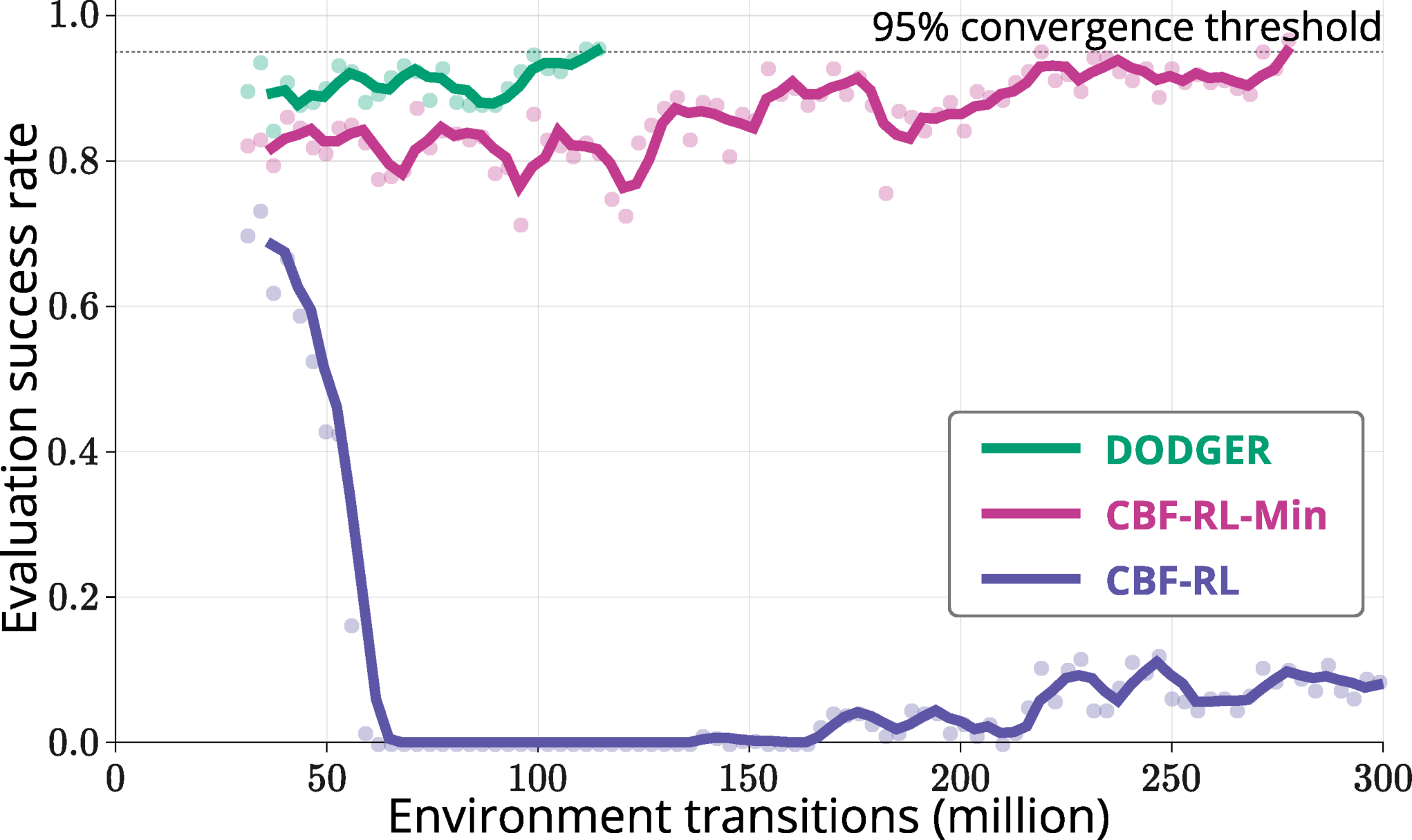
We further evaluate the methods at obstacle speeds up to $0.8\,\mathrm{m/s}$ with a $1200$-million-transition budget. DODGER converges after approximately $536$ million transitions, whereas CBF-RL-Min and CBF-RL do not converge, with final success rates of $88.5\%$ and $0.4\%$, respectively.

We compare DPCBF with the Collision Cone CBF (C3BF) [25] and a distance-based CBF under the same DODGER training configuration. C3BF incorporates relative position and velocity through $h_{\mathrm{C3}}=\langle\bm{p}_{\mathrm{rel}},\bm{v}_{\mathrm{rel}}\rangle+d(\bm{x})\lVert\bm{v}_{\mathrm{rel}}\rVert$. In contrast, the distance-based barrier is defined as $h_{\mathrm{dist}}=\lVert\bm{p}_{\mathrm{rel}}\rVert^{2}-r^{2}$. Since $h_{\mathrm{dist}}$ has relative degree two with respect to the reduced-order dynamics in (2), we enforce the distance-based safety constraint using an exponential CBF (ECBF) [26]. We additionally evaluate a distance-based ECBF variant with yaw-rate regularization to examine the large yaw commands observed with the original distance-based formulation. All other components are kept identical across the CBF variants.

Table II summarizes the training outcomes. DPCBF and both distance-based ECBF variants reach curriculum stage 3 and converge, with DPCBF requiring the fewest environment transitions. In contrast, C3BF does not converge within the training budget and reaches only stage 1.

To further characterize the yaw behavior, we compare the actor yaw commands and the resulting G1 yaw rates for DPCBF and the two distance-based ECBF variants. Over $N$ evaluated samples, the command root-mean-square (RMS) value is $\omega_{\mathrm{cmd,RMS}}=\sqrt{N^{-1}\sum_{t=1}^{N}(\omega_{t}^{\pi})^{2}}$, while the command near-saturation fraction is $f_{\mathrm{cmd,sat}}=N^{-1}\sum_{t=1}^{N}\mathmybb{1}\{|\omega_{t}^{\pi}|\geq 0.9\,\mathrm{rad/s}\}$. The G1 metrics use the measured yaw rate $\dot{\phi}_{t}$ and the same threshold; fractions are reported as percentages. As shown in Table III, the distance-based ECBF variants produce larger yaw-rate commands and more frequent near-saturation than DPCBF, both in the actor output and in the resulting G1 motion.

References

- [1] (2023) Champion-level drone racing using deep reinforcement learning. Nature 620, pp. 982–987. External Links: Document Cited by: §I.
- [2] (2024) Real-world humanoid locomotion with reinforcement learning. Science Robotics 9 (89), pp. eadi9579. Cited by: §I.
- [3] (2016) Model-predictive control with stochastic collision avoidance using bayesian policy optimization. In IEEE International Conference on Robotics and Automation (ICRA), pp. 4597–4604. External Links: Document Cited by: §I.
- [4] (2021) Collision-Free MPC for legged robots in static and dynamic scenes. In IEEE International Conference on Robotics and Automation (ICRA), pp. 8266–8272. External Links: Document Cited by: §I.
- [5] (2025) Safe quadrotor navigation using composite control barrier functions. In IEEE International Conference on Robotics and Automation (ICRA), pp. 6343–6349. External Links: Document Cited by: §I.
- [6] (2025) SHIELD: safety on humanoids via CBFs in expectation on learned dynamics. In IEEE/RSJ International Conference on Intelligent Robots and Systems (IROS), pp. 203–210. External Links: Document Cited by: §I.
- [7] (2026) Is Your Safe Controller Actually Safe? A Critical Review of CBF Tautologies and Hidden Assumptions. In arXiv preprint arXiv:2603.06954, (en). Cited by: §I.
- [8] (2024) Barrier functions inspired reward shaping for reinforcement learning. In IEEE International Conference on Robotics and Automation (ICRA), pp. 10807–10813. External Links: Document Cited by: §I.
- [9] (2026) Reinforcement learning for risk adaptation via differentiable CVaR barrier functions. arXiv preprint arXiv:2605.21257. Cited by: §I.
- [10] (2019) End-to-end safe reinforcement learning through barrier functions for safety-critical continuous control tasks. In Proceedings of the AAAI Conference on Artificial Intelligence, pp. 3387–3395. External Links: Document Cited by: §I.
- [11] (2025) Safe reinforcement learning using robust control barrier functions. IEEE Robotics and Automation Letters 10 (3), pp. 2886–2893. External Links: Document Cited by: §I.
- [12] (2025) Safety filtering while training: improving the performance and sample efficiency of reinforcement learning agents. IEEE Robotics and Automation Letters 10 (1), pp. 788–795. External Links: Document Cited by: §I.
- [13] (2026) CBF-RL: safety filtering reinforcement learning in training with control barrier functions. In IEEE International Conference on Robotics and Automation (ICRA), Cited by: §I, §II-B, §II-B, §III-C, §IV-B2.
- [14] (2026) Beyond collision cones: dynamic obstacle avoidance for nonholonomic robots via dynamic parabolic control barrier functions. In IEEE International Conference on Robotics and Automation (ICRA), Cited by: §I, §III-A2, §III-A2.
- [15] (2019) Control barrier functions: theory and applications. In European Control Conference (ECC), pp. 3420–3431. External Links: Document Cited by: §II-A.
- [16] (2026) Learning to adapt control barrier functions under epistemic and aleatoric uncertainty. In arXiv preprint arXiv:2504.03038, Cited by: §III-B.
- [17] (2024) CaT: constraints as terminations for legged locomotion reinforcement learning. In IEEE/RSJ International Conference on Intelligent Robots and Systems (IROS), pp. 13303–13310. External Links: Document Cited by: §III-C2, §IV-B1.
- [18] (2026) Scalable multi-objective robot reinforcement learning through gradient conflict resolution. In IEEE International Conference on Robotics and Automation (ICRA), Cited by: §III-C2.
- [19] (2017) Proximal policy optimization algorithms. In arXiv preprint arXiv:1707.06347, Cited by: §III-C2.
- [20] (2025) Uncertainty-aware latent safety filters for avoiding out-of-distribution failures. In Conference on Robot Learning (CoRL), Cited by: §IV-A.
- [21] (2005) A time-dependent Hamilton–Jacobi formulation of reachable sets for continuous dynamic games. IEEE Transactions on Automatic Control 50 (7), pp. 947–957. External Links: Document Cited by: §IV-A, §IV-A.
- [22] (2025) MuJoCo Playground. In arXiv preprint arXiv:2502.08844, Cited by: §IV-B1.
- [23] (2017) Detection and tracking of 2D geometric obstacles from LRF data. In International Workshop on Robot Motion and Control (RoMoCo), pp. 135–141. Cited by: §IV-B1.
- [24] (2026) PAC-MAN: perception-aware CBF-RL for whole-body safety in humanoid dodgeball. In arXiv preprint arXiv:2607.28623, Cited by: §IV-B2.
- [25] (2026) A collision cone approach for control barrier functions. IEEE Transactions on Control Systems Technology 34 (3), pp. 1297–1310. External Links: Document Cited by: §IV-B3.
- [26] (2016) Exponential control barrier functions for enforcing high relative-degree safety-critical constraints. In American Control Conference (ACC), pp. 322–328. External Links: Document Cited by: §IV-B3.
- [27] (2023) Direct LiDAR-inertial odometry: lightweight LIO with continuous-time motion correction. In IEEE International Conference on Robotics and Automation (ICRA), pp. 3983–3989. External Links: Document Cited by: §IV-D.
-A Barrier Function Derivatives and Safety Conditions
-A1 Common Notation
The obstacle index is omitted throughout this appendix for clarity. Recall that
and
Let
denote the line-of-sight (LoS) angle and define . The relative velocity expressed in the LoS frame is