An energy-based discontinuous Galerkin method for wave equations on complex geometric domains

Yangxin Fu Yan Jiang Siyang Wang Lu Zhang

Abstract

This paper develops a high-order cut energy-based discontinuous Galerkin (CutEDG) method for second-order acoustic wave equations on complex domains and across stationary material interfaces. The method employs unfitted Cartesian meshes and addresses the small-cut-cell problem by introducing ghost-penalty stabilization directly into the local bilinear forms defining the EDG energy, while leaving the original spatial coupling and numerical-flux structure unchanged. We establish semidiscrete energy stability and a priori error estimates showing that high-order accuracy is retained. The formulation is further extended to interface problems with discontinuous wave speeds. Numerical experiments confirm the predicted convergence rates and demonstrate robustness with respect to arbitrarily small cut cells. In particular, the explicit time-step restriction is governed by the background mesh size rather than the smallest physical cut cell, and the stabilized energy Gram matrices exhibit cut-independent conditioning.

Keywords: Wave equation, cutEDG method, stability, high order accuracy

AMS subject classifications 2020: 65M60, 65M85, 65M12

1 Introduction

Wave propagation in geometrically complex media arises in a broad range of applications, including acoustics, seismic modeling, nondestructive testing, and wave-structure interaction; see, for example, [16, 18, 22] and the references therein. In many of these applications, waves propagate over many wavelengths or over long time intervals, so that numerical dispersion and phase errors can accumulate significantly. High-order discretizations are therefore particularly attractive, since they can achieve a prescribed accuracy with fewer degrees of freedom per wavelength than low-order methods [1]. At the same time, practical computational domains may contain curved boundaries, embedded obstacles, or material interfaces with complicated geometry. Developing numerical methods that combine high-order accuracy with geometric flexibility is thus an important issue in computational wave propagation.

Conventional high-order finite element and discontinuous Galerkin (DG) methods typically rely on meshes that conform to the physical boundary or interface; see, e.g., [23, 30, 17]. Although body-fitted and curvilinear meshes are effective when a suitable mesh is available, their construction may become costly and technically demanding for complicated geometries, especially at high order. This difficulty becomes more pronounced when many geometric configurations have to be considered or when interfaces vary between simulations. Unfitted and immersed methods provide an attractive alternative [19, 20, 5] by embedding the physical domain in a simple background mesh, often structured or Cartesian, while allowing physical boundaries and interfaces to intersect the mesh without requiring mesh conformity.

The flexibility of an unfitted mesh, however, comes with the well-known small-cut-cell problem [8, 7, 6]. When a boundary or interface passes arbitrarily close to a mesh vertex or edge, the physical portion of a cut element can become arbitrarily small. As a consequence, discrete functions supported on such elements may receive only weak control from integration over the physical domain, leading to severe ill-conditioning and loss of uniform stability. For time-dependent wave problems, the issue is particularly important because arbitrarily small cut cells may also impose a prohibitively restrictive time-step constraint for explicit time integration. An effective unfitted wave discretization must therefore remain robust with respect to the cut configuration, including the limiting case in which the physical fraction of a cut element tends to zero.

Ghost-penalty stabilization provides a systematic mechanism for recovering such robustness and is a central ingredient of Cut Finite Element Methods (CutFEM) [7, 6]. Stabilized CutFEM formulations have been developed for elliptic, interface, and wave problems [7, 6, 25]. For wave equations, higher-order extensions have demonstrated high-order accuracy and favorable explicit stability properties on unfitted meshes [26, 27]; in particular, [26] shows numerically that the CFL restriction is essentially unaffected by the immersed boundary. Related ideas have also been extended to discontinuous finite element spaces. [13] developed a stabilized CutDG framework for elliptic boundary value and interface problems, with error and condition-number estimates that are robust with respect to the cut configuration. Ghost-penalty-based CutDG formulations have subsequently been studied for hyperbolic problems [14, 11, 9, 10]. In particular, high-order CutDG methods for hyperbolic conservation laws have shown that explicit time stepping can be performed with a time-step restriction independent of the size of the smallest cut element [11, 10]. These developments establish ghost stabilization as an effective tool for unfitted discretizations, but they do not by themselves determine how the stabilization should be incorporated into a particular wave formulation.

In this work, we consider this question within the energy-based discontinuous Galerkin (EDG) framework. DG methods are attractive for high-order wave propagation because of their local structure, high-order accuracy, and natural compatibility with explicit time integration [15]. Among the different DG formulations available for second-order wave equations (see, e.g., [28, 12, 24] and reference therein), EDG is particularly well suited to the objective of the present work because its construction is organized directly around a discrete counterpart of the wave energy (see, e.g., [3, 4, 2, 29, 21]). The mesh independent numerical fluxes can be chosen so that the semidiscrete scheme satisfies an energy-conserving or energy-dissipating relation. Thus, the energy is not only a tool for analyzing the final scheme, but also provides a natural principle for designing the discretization. This point becomes important on an unfitted mesh. In the EDG formulation, the discrete energy is associated with two local bilinear forms, one involving the gradient of the displacement variable and the other the $L^{2}$ inner product of the velocity variable. When the physical portion of an element becomes arbitrarily small, both forms lose uniform control of the degrees of freedom supported on that element. The small-cut problem therefore acts directly on the local forms that define the EDG energy. This suggests designing the cut stabilization at the level of these energy components, rather than transferring the mass-stiffness stabilization of continuous CutFEM directly to the EDG spatial operator.

Following this idea, we develop a high-order cut energy-based discontinuous Galerkin (CutEDG) method for the second-order acoustic wave equation on complex domains and across stationary material interfaces. Ghost-penalty terms are introduced into the two local bilinear forms associated with the discrete energy in the cut region, while no additional ghost penalty is added to the spatial coupling and numerical-flux terms of the original EDG formulation. The stabilization therefore restores control of the degrees of freedom on arbitrarily small cut cells without altering the underlying EDG flux structure. This construction preserves the energy mechanism that motivates the EDG formulation. More precisely, if $E_{h}(t)$ denotes the standard EDG energy on the physical domain and $D_{h}(t)\geq 0$ denotes the contribution of the cut stabilization, the semidiscrete CutEDG method satisfies an estimate of the form $\frac{\mathrm{d}}{\mathrm{d}t}\bigl(E_{h}(t)+D_{h}(t)\bigr)\leq 0$ (see (3.23)). The additional term $D_{h}$ restores the control that is lost on arbitrarily small physical intersections, so that the augmented energy remains uniformly meaningful with respect to the cut configuration. In this sense, the ghost stabilization extends the original EDG energy to the cut region while retaining its stability mechanism.

In this work, we establish stability and a priori error estimates for the proposed method and show that the designed high-order accuracy is retained. The formulation is further extended to stationary interface problems, where the interface may cut arbitrarily through the Cartesian background mesh. Numerical experiments demonstrate robustness with respect to decreasing cut-cell fractions and show that the explicit stability restriction is governed by the background mesh scale rather than by the smallest physical cut. We also numerically investigate the conditioning of the stabilized energy Gram matrices. At the polynomial orders considered, the corresponding condition numbers remain bounded with respect to the cut position and are of the same order of magnitude as, while slightly smaller than, those observed for the analogous high-order continuous CutFEM discretization, indicating favorable algebraic behavior for high-order explicit wave propagation.

The main contributions are therefore threefold. First, we develop a high-order unfitted EDG formulation for both single-domain and stationary interface wave problems on Cartesian meshes. Second, we construct a ghost stabilization tailored to the local energy form of EDG, restoring uniform control on arbitrarily small cut cells while leaving the original spatial coupling and numerical-flux structure unchanged. Third, we establish stability and high-order error estimates and demonstrate numerically cut-independent explicit stability and favorable conditioning of the stabilized discrete operators.

The remainder of this paper is organized as follows. Section 2 first reviews the energy-based discontinuous Galerkin method and develops the proposed CutEDG formulation for acoustic wave equations. Stability and a priori error estimates are established on Cartesian meshes in Section 3. Section 4 considers stationary interface problems and presents the corresponding CutEDG formulation. Section 5 provides a comprehensive set of numerical experiments to verify the theoretical convergence rates and demonstrate the accuracy, stability, and robustness of the proposed method. Finally, concluding remarks are given in Section 6.

2 The CutEDG method

In this section, we develop a cut-cell energy-based discontinuous Galerkin (CutEDG) method for the second-order wave equation. We first introduce the model problem and the background mesh, and then briefly review the energy-based discontinuous Galerkin (EDG) formulation of [3]. To handle the difficulties arising from arbitrarily small cut cells on unfitted meshes, we augment the EDG formulation with a ghost-penalty stabilization.

2.1 Model problem and fitted EDG formulation

We consider the second-order wave equation


$\displaystyle u_{tt}$	$\displaystyle=\Delta u+f(\mathbf{x},t),$	$\displaystyle\mathbf{x}\in\Omega,\quad t\in(0,T),$	(2.1a)
$\displaystyle u$	$\displaystyle=0,$	$\displaystyle\mathbf{x}\in\Gamma,\quad t\in[0,T],$	(2.1b)
$\displaystyle u(\mathbf{x},0)$	$\displaystyle=u_{0}(\mathbf{x}),\qquad u_{t}(\mathbf{x},0)=v_{0}(\mathbf{x}),$	$\displaystyle\mathbf{x}\in\Omega.$	(2.1c)

Here, $\Omega\subset\mathbb{R}^{d}$ is a bounded physical domain with boundary $\Gamma=\partial\Omega$ . The function $f$ denotes the source term, and $u_{0}$ and $v_{0}$ are the initial displacement and velocity, respectively.

Introducing the velocity variable $v=u_{t}$ , the wave equation can be written as the first-order system in time

	$\displaystyle u_{t}$	$\displaystyle=v,$		(2.2)
	$\displaystyle v_{t}$	$\displaystyle=\Delta u+f.$		(2.2)

We first recall the EDG formulation on a boundary-fitted mesh (see, e.g., [3]). This formulation serves as the reference discretization from which the cut-cell method will be constructed. Let $\mathcal{T}_{h}^{\mathrm{fit}}$ be a boundary-fitted tessellation of $\Omega$ into non-overlapping elements $K$ such that $\overline{\Omega}=\bigcup_{K\in\mathcal{T}_{h}^{\mathrm{fit}}}\overline{K}$ . For polynomial degrees $p$ and $q$ , define the approximation spaces

	$\displaystyle U_{h,\mathrm{fit}}^{p}$	$\displaystyle=\left\{w_{h}:w_{h}\in\mathcal{P}^{p}(K)\quad\forall K\in\mathcal{T}_{h}^{\mathrm{fit}}\right\},$		(2.3)
	$\displaystyle V_{h,\mathrm{fit}}^{q}$	$\displaystyle=\left\{w_{h}:w_{h}\in\mathcal{P}^{q}(K)\quad\forall K\in\mathcal{T}_{h}^{\mathrm{fit}}\right\}.$		(2.3)

Here, $\mathcal{P}^{r}(K)$ denotes the polynomial approximation space of degree $r$ on $K$ . Depending on the element type, $\mathcal{P}^{r}(K)$ may denote either total-degree polynomials or the corresponding tensor-product polynomial space.

Motivated by the continuous energy of the wave equation, the EDG scheme considers the discrete energy

E_{h}(t)=\frac{1}{2}\sum_{K\in\mathcal{T}_{h}^{\mathrm{fit}}}\int_{K}\left(|v_{h}|^{2}+|\nabla u_{h}|^{2}\right)\,d\mathbf{x},

(2.4)

and constructs the spatial discretization retains such discrete energy structure. Specifically, on each element $K\in\mathcal{T}_{h}^{\mathrm{fit}}$ , one seeks $(u_{h},v_{h})\in U_{h,\mathrm{fit}}^{p}\times V_{h,\mathrm{fit}}^{q}$ such that, for all $(\phi_{u},\phi_{v},\widetilde{\phi})\in U_{h,\text{fit}}^{p}(K)\times U_{h,\text{fit}}^{q}(K)\times U_{h,\text{fit}}^{0}(K)$ ,


$\displaystyle\int_{K}\widetilde{\phi}\big((u_{h})_{t}-v_{h}\big)\,d\mathbf{x}$	$\displaystyle=0,$	(2.5a)
$\displaystyle\int_{K}\nabla\phi_{u}\cdot\nabla\big((u_{h})_{t}-v_{h}\big)\,d\mathbf{x}$	$\displaystyle=\int_{\partial K}(\widehat{v_{h}}-v_{h})\nabla\phi_{u}\cdot\mathbf{n}\,dS,$	(2.5b)
$\displaystyle\int_{K}\phi_{v}(v_{h})_{t}+\nabla\phi_{v}\cdot\nabla u_{h}\,d\mathbf{x}$	$\displaystyle=\int_{\partial K}\phi_{v}\,\widehat{\nabla u_{h}}\cdot\mathbf{n}\,dS+\int_{K}\phi_{v}f\,d\mathbf{x},.$	(2.5c)

Here, $\mathbf{n}$ denotes the outward unit normal to $\partial K$ . To define the numerical fluxes, consider an interior face shared by two neighboring elements $K^{+}$ and $K^{-}$ . For a scalar or vector-valued discrete function $w$ , we denote by $w^{\pm}$ its traces on $F$ taken from the interior of $K^{\pm}$ , respectively. Let $\mathbf{n}^{\pm}$ be the outward unit normals to $K^{\pm}$ on $F$ , so that $\mathbf{n}^{-}=-\mathbf{n}^{+}$ . For a scalar quantity $w$ and a vector quantity $\mathbf{q}$ , we define the corresponding normal jumps by

[\![w]\!]=w^{+}\mathbf{n}^{+}+w^{-}\mathbf{n}^{-},\qquad[\![\mathbf{q}]\!]=\mathbf{q}^{+}\cdot\mathbf{n}^{+}+\mathbf{q}^{-}\cdot\mathbf{n}^{-}.

(2.6)

In particular,

[\![\nabla u_{h}]\!]=\nabla u_{h}^{+}\cdot\mathbf{n}^{+}+\nabla u_{h}^{-}\cdot\mathbf{n}^{-}.

The numerical fluxes on an interior face are taken as

	$\displaystyle\widehat{v_{h}}$	$\displaystyle=\alpha v_{h}^{+}+(1-\alpha)v_{h}^{-}-\tau[\![\nabla u_{h}]\!],$		(2.7)
	$\displaystyle\widehat{\nabla u_{h}}$	$\displaystyle=(1-\alpha)\nabla u_{h}^{+}+\alpha\nabla u_{h}^{-}-\beta[\![v_{h}]\!].$		(2.7)

The parameters $\alpha$ , $\tau$ , and $\beta$ determine the particular choice of numerical flux. On the physical boundary $\Gamma$ , the boundary numerical fluxes are defined consistently with the prescribed homogeneous Dirichlet data, namely,

\widehat{v_{h}}=0,\qquad\widehat{\nabla u_{h}}=\nabla u_{h}.

(2.8)

We note that (2.5b) controls only the gradient of $(u_{h})_{t}-v_{h}$ and therefore leaves its elementwise constant component undetermined. The additional relation (2.5a) determines this constant mode by enforcing the corresponding elementwise mean condition. Thus, (2.5b) and (2.5a) together provide a complete discrete representation of the relation $u_{t}=v$ .

The formulation above assumes that the computational mesh conforms to the physical boundary. We next remove this restriction by embedding $\Omega$ into a Cartesian background mesh and restricting the physical integrals to the portions of the background cells lying inside $\Omega$ .

2.2 Background mesh and cut-cell geometry

Let $\widetilde{\mathcal{T}}_{h}$ be a Cartesian background mesh covering the physical domain $\Omega$ . The mesh is constructed independently of the physical boundary $\Gamma=\partial\Omega$ , so that $\Gamma$ may intersect the background cells without conforming to their faces. We denote a generic background cell by $K$ and define

h_{K}=\operatorname{diam}(K),\qquad h=\max_{K\in\widetilde{\mathcal{T}}_{h}}h_{K}.

The discretization is supported only on those background cells having a nonzero intersection with the physical domain. This defines the active mesh and its associated computational domain,

\mathcal{T}_{h}=\left\{K\in\widetilde{\mathcal{T}}_{h}:|K\cap\Omega|>0\right\},\qquad\Omega_{h}=\bigcup_{K\in\mathcal{T}_{h}}K.

(2.9)

For each $K\in\mathcal{T}_{h}$ , we denote its physical part by

K_{\Omega}:=K\cap\Omega.

(2.10)

Thus, although the discrete functions are represented on the full background cell $K$ , the physical-domain contributions are evaluated only over $K_{\Omega}$ . The active mesh $\mathcal{T}_{h}$ is naturally decomposed according to the interaction of its cells with the physical boundary. We define

\mathcal{T}_{h}^{\mathrm{int}}=\left\{K\in\mathcal{T}_{h}:\overline{K}\subset\Omega\right\},\qquad\mathcal{T}_{h}^{\Gamma}=\mathcal{T}_{h}\setminus\mathcal{T}_{h}^{\mathrm{int}}.

(2.11)

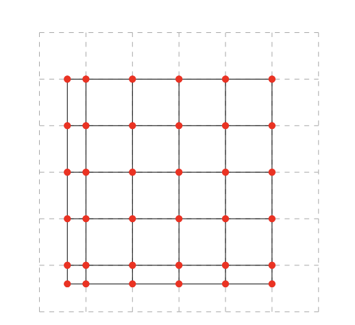
Cells in $\mathcal{T}_{h}^{\mathrm{int}}$ are unaffected by the geometric cut and satisfy $K_{\Omega}=K$ , whereas cells in $\mathcal{T}_{h}^{\Gamma}$ are intersected by the physical boundary and generally satisfy $K_{\Omega}\subsetneq K$ . See Figure 2.1 for an illustration in 2D.

Figure 2.1: Illustration of an unfitted two-dimensional discretization. The physical domain

\Omega

is bounded by

\Gamma

and embedded in the Cartesian background mesh

\widetilde{\mathcal{T}}_{h}

. The blue cells are the interior cells fully contained in

\Omega

, whereas the green cells are the cut cells intersected by

\Gamma

, denoted as

\mathcal{T}_{h}^{\mathrm{int}}

and

\mathcal{T}^{\Gamma}_{h}

respectively. The union of the interior and cut cells forms the computational mesh

\mathcal{T}_{h}

used for the discretization of

\Omega

To distinguish the interfaces associated with the background mesh from those induced by the physical boundary, let

\mathcal{F}_{h}^{\mathrm{int}}=\left\{F=\partial K^{+}\cap\partial K^{-}:K^{\pm}\in\mathcal{T}_{h}\,;\,\operatorname{meas}_{d-1}(F)>0\right\}

(2.12)

be the set of interior faces of the active background mesh. Only the parts of these faces lying inside $\Omega$ enter the physical EDG fluxes; we therefore introduce

\mathcal{F}_{h}^{\Omega}=\left\{F\cap\Omega:F\in\mathcal{F}_{h}^{\mathrm{int}}\,;\,\operatorname{meas}_{d-1}(F\cap\Omega)>0\right\}.

(2.13)

The portions of the physical boundary contained in the cut cells are collected in

\mathcal{F}_{h}^{\Gamma}=\left\{K\cap\Gamma:K\in\mathcal{T}_{h}^{\Gamma}\,;\,\operatorname{meas}_{d-1}(K\cap\Gamma)>0\right\}.

(2.14)

Hence, three geometric objects play distinct roles in the CutEDG formulation: $K_{\Omega}$ determines the physical volume integrals, $\mathcal{F}_{h}^{\Omega}$ determines the numerical fluxes between neighboring active cells, and $\mathcal{F}_{h}^{\Gamma}$ represents the true physical boundary on which the boundary condition is imposed. This distinction will also be useful when introducing the ghost-penalty stabilization, which is defined instead on selected full background faces.

2.3 CutEDG discretization

We now extend the fitted EDG formulation (2.5) to the active background mesh $\mathcal{T}_{h}$ . The discrete functions are represented by polynomials on the entire background cells, while the physical volume and boundary integrals are restricted to the intersections with $\Omega$ . We define the approximation spaces on the active mesh by

	$\displaystyle U_{h}^{p}$	$\displaystyle=\left\{w_{h}:w_{h}\in\mathcal{P}^{p}(K)\quad\forall K\in\mathcal{T}_{h}\right\},$		(2.15)
	$\displaystyle V_{h}^{q}$	$\displaystyle=\left\{w_{h}:w_{h}\in\mathcal{P}^{q}(K)\quad\forall K\in\mathcal{T}_{h}\right\}.$		(2.15)

The unstabilized CutEDG formulation is obtained by replacing each fitted element $K$ in (2.5) by its physical portion $K_{\Omega}$ defined in (2.10). Thus, for every $K\in\mathcal{T}_{h}$ , we seek $(u_{h},v_{h})\in U_{h}^{p}\times V_{h}^{q}$ such that, for all $(\phi_{u},\phi_{v},\widetilde{\phi})\in U_{h}^{p}\times V_{h}^{q}\times U_{h}^{0}$ ,


$\displaystyle\int_{K_{\Omega}}\widetilde{\phi}\big((u_{h})_{t}-v_{h}\big)\,d\mathbf{x}$	$\displaystyle=0,$	(2.16a)
$\displaystyle\int_{K_{\Omega}}\nabla\phi_{u}\cdot\nabla\big((u_{h})_{t}-v_{h}\big)\,d\mathbf{x}$	$\displaystyle=\int_{\partial K_{\Omega}}(\widehat{v_{h}}-v_{h})\nabla\phi_{u}\cdot\mathbf{n}_{\Omega,K}\,dS,$	(2.16b)
$\displaystyle\int_{K_{\Omega}}\phi_{v}(v_{h})_{t}+\nabla\phi_{v}\cdot\nabla u_{h}\,d\mathbf{x}$	$\displaystyle=\int_{\partial K_{\Omega}}\phi_{v}\widehat{\nabla u_{h}}\cdot\mathbf{n}_{\Omega,K}\,dS+\int_{K_{\Omega}}\phi_{v}f\,d\mathbf{x},.$	(2.16c)

Here, $\mathbf{n}_{\Omega,K}$ denotes the outward unit normal to the physical cell $K_{\Omega}$ . On a physical interior face belonging to $\mathcal{F}_{h}^{\Omega}$ , the numerical fluxes are inherited directly from the fitted EDG formulation. On a boundary segment belonging to $\mathcal{F}_{h}^{\Gamma}$ , the numerical fluxes are replaced by the corresponding boundary fluxes used to impose the prescribed homogeneous Dirichlet condition.

For an interior cell $K\in\mathcal{T}_{h}^{\mathrm{int}}$ , one has $K_{\Omega}=K$ . Consequently, the local CutEDG equations reduce exactly to the fitted EDG equations. The distinction arises only in the vicinity of the physical boundary, where the measure of $K_{\Omega}$ may be arbitrarily small relative to that of the background cell $K$ .

2.4 Small-cut-cell problem and ghost-penalty stabilization

To characterize the position of the physical boundary within an active cell, we define the volume fraction

\eta_{K}=\frac{|K_{\Omega}|}{|K|},\qquad K\in\mathcal{T}_{h}.

(2.17)

For an interior cell, $\eta_{K}=1$ , whereas for a cut cell $\eta_{K}\in(0,1)$ and may become arbitrarily small as the location of $\Gamma$ changes relative to the background grid. When $\eta_{K}\ll 1$ , the physical volume contributions associated with $K$ become small, even though the discrete polynomial on $K$ is still represented by degrees of freedom defined over the full background cell. As a consequence, the discrete system (2.16) may lose uniform control of modes supported predominantly in the fictitious portion $K\setminus\Omega$ . This is the familiar small-cut-cell problem and may lead to severe deterioration of the conditioning of the resulting algebraic system.

To restore control in the cut region, motivated by [26], we introduce a ghost-penalty stabilization on background faces adjacent to cut cells. Define

\mathcal{F}_{h}^{g}=\left\{F=\partial K^{+}\cap\partial K^{-}\in\mathcal{F}_{h}^{\mathrm{int}}:K^{+}\in\mathcal{T}_{h}^{\Gamma}\text{ or }K^{-}\in\mathcal{T}_{h}^{\Gamma}\right\}.

(2.18)

An important distinction is that the stabilization is integrated over the full background face $F$ , rather than only over its physical portion $\Omega_{F}=F\cap\Omega$ . The ghost penalty therefore transfers control from the physical domain into the neighboring fictitious parts of the active mesh. Precisely, for a polynomial degree $r$ , define

J_{r}(w,z)=\sum_{F\in\mathcal{F}_{h}^{g}}\sum_{\ell=0}^{r}\omega_{\ell}\frac{h^{2\ell+1}}{(2\ell+1)(\ell!)^{2}}\int_{F}[\![\partial_{n_{F}}^{\ell}w]\!]\,[\![\partial_{n_{F}}^{\ell}z]\!]\,dS,

(2.19)

where $n_{F}$ is a fixed unit normal associated with $F$ , $\partial_{n_{F}}^{\ell}$ denotes the $\ell$ th-order directional derivative in the $n_{F}$ direction, and $\omega_{\ell}>0$ is a stabilization weight. Since the approximation spaces are discontinuous, the contribution with $\ell=0$ is retained and penalizes jumps of the discrete functions themselves.

Because $J_{r}(\cdot,\cdot)$ is defined as a sum over background faces, it is most naturally interpreted as a global stabilization form. Accordingly, the stabilized CutEDG formulation is obtained by adding the appropriate ghost-penalty contributions to the assembled CutEDG equations. In abstract form, the two evolution equations may be written as

		$\displaystyle\sum_{K\in\mathcal{T}_{h}}\int_{K_{\Omega}}\nabla\phi_{u}\cdot\nabla\big((u_{h})_{t}-v_{h}\big)\,d\mathbf{x}+\gamma_{M}^{u}h^{-2}J_{p}\big((u_{h})_{t},\phi_{u}\big)$		(2.20)
	$\displaystyle=$	$\displaystyle\sum_{K\in\mathcal{T}_{h}}\int_{\partial K_{\Omega}}(\widehat{v_{h}}-v_{h})\nabla\phi_{u}\cdot\mathbf{n}_{\Omega,K}\,dS,$		(2.20)

and

		$\displaystyle\sum_{K\in\mathcal{T}_{h}}\int_{K_{\Omega}}\left(\phi_{v}(v_{h})_{t}+\nabla\phi_{v}\cdot\nabla u_{h}\right)\,d\mathbf{x}+\gamma_{M}^{v}J_{q}\big((v_{h})_{t},\phi_{v}\big)$		(2.21)
	$\displaystyle=$	$\displaystyle\sum_{K\in\mathcal{T}_{h}}\int_{\partial K_{\Omega}}\phi_{v}\widehat{\nabla u_{h}}\cdot\mathbf{n}_{\Omega,K}\,dS+\sum_{K\in\mathcal{T}_{h}}\int_{K_{\Omega}}\phi_{v}f\,d\mathbf{x}.$		(2.21)

The element-wise mean condition associated with the relation $u_{t}=v$ is imposed in the stabilized formulation as

\sum_{K\in\mathcal{T}_{h}}\int_{K_{\Omega}}h^{-2}\widetilde{\phi}\big((u_{h})_{t}-v_{h}\big)\,d{\bf x}+\gamma_{M}^{u}h^{-2}J_{p}\big((u_{h})_{t},\widetilde{\phi}\big)=0.

(2.22)

We note that the global form (2.20)–(2.22) makes explicit that each ghost face contributes only once to the assembled system. Nevertheless, the resulting couplings remain local: the physical volume terms involve individual physical cells $K_{\Omega}$ , the numerical fluxes couple neighboring elements across the relevant portions of $\partial K_{\Omega}$ , and the ghost-penalty terms couple only pairs of elements sharing a face in $\mathcal{F}_{h}^{g}$ . Consequently, cells away from the cut region receive no ghost-penalty contribution, and their discretization coincides with the fitted EDG scheme.

Remark 2.1.

The gradient equation does not control the elementwise constant component of $(u_{h})_{t}-v_{h}$ . The mean-value condition is therefore a complementary algebraic constraint required to determine this otherwise undetermined mode. To incorporate this constraint consistently into the stabilized formulation, the mean equation (2.16a) is first scaled by $h^{-2}$ . A ghost-penalty term acting on $(u_{h})_{t}$ is then added with the same $h^{-2}$ scaling as in (2.20). This scaling places the mean constraint on the same dimensional level as the gradient equation and provides additional control of the constant mode in the cut region (see (2.22)). Nonetheless, since $\widetilde{\phi}$ is piecewise constant, only the zeroth-order contribution of $J_{p}\big((u_{h})_{t},\widetilde{\phi}\big)$ is nonzero.

Remark 2.2.

The ghost penalty introduces additional coupling only across faces in $\mathcal{F}_{h}^{g}$ . Hence, the coupling induced by the cut-cell stabilization is confined to a neighborhood of the physical boundary. Away from this region, the discrete operator retains the same element-local structure as the fitted EDG method. In particular, the ghost penalty modifies only the part of the discrete system associated with cut cells and their neighboring elements.

Remark 2.3.

The CutEDG formulation (2.16) inherits its underlying structure from the EDG discretization (2.5). In particular, the physical-domain terms retain the same energy structure as in the fitted formulation. The ghost-penalty terms introduce additional stabilization in the cut region, and their contribution to the discrete energy balance depends on the particular stabilization operators and numerical fluxes. The resulting energy properties of the stabilized CutEDG formulation are therefore analyzed separately below.

3 Stability and error analysis

In this section, we analyze the stability and convergence of the proposed CutEDG method (2.20)–(2.22). We first establish a semi-discrete energy estimate and then derive an a priori error bound.

3.1 Discrete energy stability

We begin with the homogeneous problem, for which the source term and Dirichlet boundary data vanish. The main stability result is stated below.

Theorem 3.1.

Assume that $f=0$ , and let $\tau,\beta\geq 0$ . Then the semi-discrete CutEDG solution obtained from (2.20)–(2.22) satisfies

\frac{d}{dt}\left(E_{h}(t)+\gamma_{M}^{(u)}h^{-2}J_{p}(u_{h},u_{h})+\gamma_{M}^{(v)}J_{q}(v_{h},v_{h})\right)\leq 0,

(3.23)

where the discrete energy is defined by

E_{h}(t)=\frac{1}{2}\sum_{K\in\mathcal{T}_{h}}\int_{K_{\Omega}}|\nabla u_{h}|^{2}+|v_{h}|^{2}\,d\mathbf{x}.

(3.24)

Proof.

By the construction (2.19), the ghost-penalty forms are symmetric and nonnegative,

J_{p}(w,w)\geq 0,\qquad J_{q}(w,w)\geq 0.

It therefore follows directly from (3.24) that $E_{h}(t)\geq 0$ .

For each $K\in\mathcal{T}_{h}$ , we choose $\phi_{u}=u_{h}$ and $\phi_{v}=v_{h}$ in the stabilized global CutEDG formulation (2.20)–(2.21), and sum the resulting equations. By symmetry of the ghost-penalty forms,

J_{p}((u_{h})_{t},u_{h})=\frac{1}{2}\frac{d}{dt}J_{p}(u_{h},u_{h}),\quad J_{q}((v_{h})_{t},v_{h})=\frac{1}{2}\frac{d}{dt}J_{q}(v_{h},v_{h}).

(3.25)

The volume coupling terms cancel after summation, giving

		$\displaystyle\frac{d}{dt}\left(E_{h}(t)+\gamma_{M}^{(u)}h^{-2}J_{p}(u_{h},u_{h})+\gamma_{M}^{(v)}J_{q}(v_{h},v_{h})\right)$		(3.26)
	$\displaystyle=$	$\displaystyle\sum_{K\in\mathcal{T}_{h}}\int_{\partial K_{\Omega}}(\widehat{v_{h}}-v_{h})\nabla u_{h}\cdot\mathbf{n}+\widehat{\nabla u_{h}}\cdot\mathbf{n}v_{h}\,dS.$		(3.26)

Using the numerical fluxes defined in (2.7) and combining the contributions from the two elements sharing each physical interior face yields

		$\displaystyle\frac{d}{dt}\left(E_{h}(t)+\gamma_{M}^{(u)}h^{-2}J_{p}(u_{h},u_{h})+\gamma_{M}^{(v)}J_{q}(v_{h},v_{h})\right)$		(3.27)
	$\displaystyle=$	$\displaystyle-\sum_{F\in\mathcal{F}_{h}^{\Omega}}\int_{F}\tau[\![\nabla u_{h}]\!]^{2}\,dS+\beta\|[\![v_{h}]\!]\|^{2}\,dS.$		(3.27)

Since $\tau,\beta\geq 0$ , we obtain (3.23), which completes the proof. ∎

3.2 A priori error estimate

We next derive an a priori error estimate for the semi-discrete CutEDG approximation (2.20)–(2.22). For the projection argument below, we assume that the exact solution admits sufficiently smooth extensions to a neighborhood containing the active domain $\Omega_{h}$ , and we use the same notation for these extensions.

Theorem 3.2.

Consider the homogeneous problem $f=0$ . Assume that

u,u_{t}\in H^{p+1}(\Omega),\qquad v,v_{t}\in H^{q+1}(\Omega),

with the corresponding norms uniformly bounded for $t\in[0,T]$ . Suppose further that

p-2\leq q\leq p

(3.28)

and that the initial discrete solution is chosen using the projections introduced below. Then

	$\displaystyle\\|\nabla(u-u_{h})\\|_{L^{2}(\Omega)}^{2}+\\|v-v_{h}\\|_{L^{2}(\Omega)}^{2}\lesssim$	$\displaystyle h^{2\gamma}\left(\|u\|_{H^{p+1}(\Omega)}^{2}+\|v\|_{H^{q+1}(\Omega)}^{2}\right)$		(3.29)
		$\displaystyle+h^{2p}\|u_{t}\|_{H^{p+1}(\Omega)}^{2}+h^{2(q+1)}\|v_{t}\|_{H^{q+1}(\Omega)}^{2},$		(3.29)

where $\gamma=\min\{p^{\prime},q^{\prime}\}$ , with

p^{\prime}=\begin{cases}p-1,&\tau=0,\\ p-\dfrac{1}{2},&\tau>0,\end{cases}\qquad q^{\prime}=\begin{cases}q,&\beta=0,\\ q+\dfrac{1}{2},&\beta>0.\end{cases}

(3.30)

Here and below, $A\lesssim B$ means that $A\leq CB$ for a constant $C>0$ independent of $h$ .

Proof.

Let $\mathcal{U}=(u,v),\mathcal{U}_{h}=(u_{h},v_{h})$ , and $\Phi=(\phi_{u},\phi_{v})\in U_{h}^{p}\times V_{h}^{q}$ . For convenience, we introduce the global residual form associated with the two energy equations of the CutEDG scheme,

$\displaystyle B_{h}(\mathcal{U}_{h},\Phi):=$	$\displaystyle\sum_{K\in\mathcal{T}_{h}}\int_{K_{\Omega}}\nabla\big((u_{h})_{t}-v_{h}\big)\cdot\nabla\phi_{u}+(v_{h})_{t}\phi_{v}+\nabla u_{h}\cdot\nabla\phi_{v}\,d\mathbf{x}$	(3.31)
	$\displaystyle-\sum_{K\in\mathcal{T}_{h}}\int_{\partial(K\cap\Omega)}(\widehat{v_{h}}-v_{h})(\nabla\phi_{u}\cdot\mathbf{n})+(\widehat{\nabla u_{h}}\cdot\mathbf{n})\phi_{v}\,dS$
	$\displaystyle+\gamma_{M}^{(u)}h^{-2}J_{p}((u_{h})_{t},\phi_{u})+\gamma_{M}^{(v)}J_{q}((v_{h})_{t},\phi_{v}).$

The elementwise mean constraint for $(u_{h})_{t}-v_{h}$ does not enter the energy argument and is therefore omitted from $B_{h}$ . By consistency of the numerical fluxes and the ghost-penalty terms, the exact and numerical solutions satisfy

B_{h}(\mathcal{U},\Phi)=0,\qquad B_{h}(\mathcal{U}_{h},\Phi)=0.

Hence the error $U-U_{h}$ satisfies

B_{h}(\mathcal{U}-\mathcal{U}_{h},\Phi)=0\qquad\forall\Phi\in U_{h}^{p}\times V_{h}^{q}.

(3.32)

To estimate the error $\mathcal{U}-\mathcal{U}_{h}$ , we compare the CutEDG solution $\mathcal{U}_{h}$ with suitablie projections of the exact solution $\mathcal{U}$ . In particular, we define the projections $(\tilde{u}_{h},\tilde{v}_{h})\in U_{h}^{p}\times V_{h}^{q}$ by

\int_{K_{\Omega}}\nabla(u-\tilde{u}_{h})\cdot\nabla\phi_{u}\,d\mathbf{x}=0,\quad\int_{K_{\Omega}}(v-\tilde{v}_{h})\phi_{v}\ d{\bf x}=0,\quad\int_{K_{\Omega}}u-\tilde{u}_{h}\,d\mathbf{x}=0,

(3.33)

for all $(\phi_{u},\phi_{v})\in U_{h}^{p}\times V_{h}^{q}$ . We now split the errors as

	$\displaystyle e_{u}:=u-u_{h}$	$\displaystyle=\tilde{e}_{u}-\delta_{u},$	$\displaystyle\tilde{e}_{u}$	$\displaystyle:=\tilde{u}_{h}-u_{h},$	$\displaystyle\delta_{u}$	$\displaystyle:=\tilde{u}_{h}-u,$		(3.34)
	$\displaystyle e_{v}:=v-v_{h}$	$\displaystyle=\tilde{e}_{v}-\delta_{v},$	$\displaystyle\tilde{e}_{v}$	$\displaystyle:=\tilde{v}_{h}-v_{h},$	$\displaystyle\delta_{v}$	$\displaystyle:=\tilde{v}_{h}-v.$		(3.34)

Substituting (3.34) into (3.32) gives

B_{h}((\tilde{e}_{u},\tilde{e}_{v}),\Phi)=B_{h}((\delta_{u},\delta_{v}),\Phi).

(3.35)

Choose $\Phi=(\tilde{e}_{u},\tilde{e}_{v})$ and invoke (3.31), we obtain

	$\displaystyle\dfrac{1}{2}\dfrac{d}{dt}\bigg(\sum_{K\in\mathcal{T}_{h}}\int_{K_{\Omega}}\|\nabla\tilde{e}_{u}\|^{2}+\tilde{e}_{v}^{2}\,d\mathbf{x}+\gamma_{M}^{(u)}h^{-2}J(\tilde{e}_{u},\tilde{e}_{u})+\gamma_{M}^{(v)}J(\tilde{e}_{v},\tilde{e}_{v})\bigg)$	(3.36)
$\displaystyle=$	$\displaystyle\underbrace{-\sum_{F\in\mathcal{F}_{h}^{\Omega}}\int_{F}[\![\nabla\tilde{e}_{u}]\!]\,\widehat{\delta_{v}}+[\![\tilde{e}_{v}]\!]\cdot\widehat{\nabla\delta_{u}}+\beta[\![\tilde{e}_{v}]\!]^{2}+\tau[\![\nabla\tilde{e}_{u}]\!]^{2}\,dS}_{\mathcal{R}_{\mathrm{flux}}}$
	$\displaystyle+\gamma_{M}^{(u)}h^{-2}J\big((\delta_{u})_{t},\tilde{e}_{u}\big)+\gamma_{M}^{(v)}J\big((\delta_{v})_{t},\tilde{e}_{v}\big),$

where we have used projection orthogonality to the volume integrals in $B_{h}((\delta_{u},\delta_{v}),(\tilde{e}_{u},\tilde{e}_{v}))$ . To estimate the right-hand-side of (3.36), similar to [3], the approximation properties of the projection defined in (3.33), together with (3.28) and standard trace estimates yield

\mathcal{R}_{\mathrm{flux}}\lesssim\|\nabla\tilde{e}_{u}\|_{L^{2}(\Omega)}^{2}+\|\tilde{e}_{v}\|_{L^{2}(\Omega)}^{2}+h^{2p^{\prime}}|u|_{H^{p+1}(\Omega)}^{2}+h^{2q^{\prime}}|v|_{H^{q+1}(\Omega)}^{2},

(3.37)

where $p^{\prime}$ and $q^{\prime}$ are given by (3.30). Additionally, for the stabilization terms in (3.36), we have

$\displaystyle\gamma_{M}^{(u)}h^{-2}J((\delta_{u})_{t},\tilde{e}_{u})\lesssim$	$\displaystyle\gamma_{M}^{(u)}h^{-2}\sum_{F\in\mathcal{F}_{h}^{g}}\sum_{k=0}^{p}w_{k}\dfrac{h^{2k+1}}{(2k+1)(k!)^{2}}\int_{F}\|[\![\partial_{n_{F}}^{k}(\delta_{u})_{t}]\!]\|^{2}+\|[\![\partial_{n_{F}}^{k}\tilde{e}_{u}]\!]\|^{2}\,dS$	(3.38)
$\displaystyle\lesssim$	$\displaystyle h^{-2}\sum_{F\in\mathcal{F}_{h}^{g}}\sum_{k=0}^{p}w_{k}h^{2k+1}h^{2(p+1)-2k-1}\|u_{t}\|^{2}_{H^{p+1}(\Omega)}+\gamma_{M}^{(u)}h^{-2}J(\tilde{e}_{u},\tilde{e}_{u})$
$\displaystyle\lesssim$	$\displaystyle h^{2p}\|u_{t}\|^{2}_{H^{p+1}(\Omega)}+\gamma_{M}^{(u)}h^{-2}J(\tilde{e}_{u},\tilde{e}_{u}).$

and

$\displaystyle\gamma_{M}^{(v)}J((\delta_{v})_{t},\tilde{e}_{v})\lesssim$	$\displaystyle\gamma_{M}^{(v)}\sum_{F\in\mathcal{F}_{h}^{g}}\sum_{k=0}^{q}w_{k}\dfrac{h^{2k+1}}{(2k+1)(k!)^{2}}\int_{F}\|[\![\partial_{n_{F}}^{k}(\delta_{v})_{t}]\!]\|^{2}+\|[\![\partial_{n_{F}}^{k}\tilde{e}_{v}]\!]\|^{2}\,dS$	(3.39)
$\displaystyle\lesssim$	$\displaystyle\sum_{F\in\mathcal{F}_{h}^{g}}\sum_{k=0}^{q}w_{k}h^{2k+1}h^{2(q+1)-2k-1}\|v_{t}\|^{2}_{H^{q+1}(\Omega)}+\gamma_{M}^{(v)}J(\tilde{e}_{v},\tilde{e}_{v})$
$\displaystyle\lesssim$	$\displaystyle h^{2(q+1)}\|v_{t}\|^{2}_{H^{q+1}(\Omega)}+\gamma_{M}^{(v)}J(\tilde{e}_{v},\tilde{e}_{v}).$

Plugging (3.37)–(3.39) into (3.36), we get

	$\displaystyle\dfrac{1}{2}\dfrac{d}{dt}\left(\sum_{K}\int_{K_{\Omega}}\|\nabla\tilde{e}_{u}\|^{2}+\tilde{e}_{v}^{2}\,d\mathbf{x}+\gamma_{M}^{(u)}h^{-2}J(\tilde{e}_{u},\tilde{e}_{u})+\gamma_{M}^{(v)}J(\tilde{e}_{v},\tilde{e}_{v})\right)$	(3.40)
$\displaystyle\lesssim$	$\displaystyle\sum_{K}\int_{K_{\Omega}}\|\nabla\tilde{e}_{u}\|^{2}+\tilde{e}_{v}^{2}\,d\mathbf{x}+\gamma_{M}^{(u)}h^{-2}J(\tilde{e}_{u},\tilde{e}_{u})+\gamma_{M}^{(v)}J(\tilde{e}_{v},\tilde{e}_{v})$
	$\displaystyle+h^{2\gamma}\left(\|u\|^{2}_{H^{p+1}(\Omega)}+\|v\|^{2}_{H^{q+1}(\Omega)}\right)+h^{2p}\|u_{t}\|^{2}_{H^{p+1}(\Omega)}+h^{2(q+1)}\|v_{t}\|^{2}_{H^{q+1}(\Omega)}.$

Since the discrete initial data are chosen from the corresponding projections, the discrete component of the initial error vanishes. Applying Gronwall’s inequality to (3.40) therefore yields

		$\displaystyle\\|\nabla\tilde{e}_{u}\\|_{L^{2}(\Omega)}^{2}+\\|\tilde{e}_{v}\\|_{L^{2}(\Omega)}^{2}+\gamma_{M}^{(u)}h^{-2}J_{p}(\tilde{e}_{u},\tilde{e}_{u})+\gamma_{M}^{(v)}J_{q}(\tilde{e}_{v},\tilde{e}_{v})$		(3.41)
	$\displaystyle\lesssim$	$\displaystyle h^{2\gamma}\left(\|u\|_{H^{p+1}(\Omega)}^{2}+\|v\|_{H^{q+1}(\Omega)}^{2}\right)+h^{2p}\|u_{t}\|_{H^{p+1(\Omega)}}^{2}+h^{2(q+1)}\|v_{t}\|_{H^{q+1}(\Omega)}^{2}.$		(3.41)

Finally, combining this estimate with the approximation properties of the projections and applying the triangle inequality gives (3.29). ∎

Remark 3.1.

The restriction (3.28) is imposed solely for the derivation of the error estimate; no corresponding relation between the polynomial degrees $p$ and $q$ is required for the stability of the scheme. In our numerical experiments, the choice $q=p-1$ yields particularly robust results, consistent with commonly used polynomial-degree combinations in standard EDG formulations (see, e.g., [3]). Moreover, for this choice of polynomial degrees, the suboptimal convergence rate stated in Theorem 3.2 can be improved to the optimal rate with special designed numerical fluxes by employing suitably constructed projection operators for which the relevant projection errors vanish on element boundaries. We refer to [3] for the corresponding analysis.

4 Interface problems

We now extend the CutEDG formulation to wave propagation problems with discontinuous wave speeds across an internal material interface. Such transmission problems arise naturally in acoustic and seismic wave propagation through heterogeneous media. When the material interface has a complicated geometry, requiring the computational mesh to conform to the interface can lead to substantial mesh-generation costs. We therefore retain the unfitted framework developed in the preceding sections and employ a Cartesian background mesh whose construction is independent of the interface location.

4.1 Model problem and interface coupling

Let the physical domain $\Omega$ be decomposed into two non-overlapping subdomains $\Omega_{1}$ and $\Omega_{2}$ such that $\overline{\Omega}=\overline{\Omega}_{1}\cup\overline{\Omega}_{2}$ , $\Omega_{1}\cap\Omega_{2}=\emptyset$ , with the internal interface $\Gamma_{I}=\partial\Omega_{1}\cap\partial\Omega_{2}$ . For $i=1,2$ , let $u_{i}$ denote the wave field in $\Omega_{i}$ , and let $c_{i}>0$ denote the corresponding constant wave speed. In each subdomain, we consider

(u_{i})_{tt}=c_{i}^{2}\Delta u_{i}+f_{i},\qquad(\mathbf{x},t)\in\Omega_{i}\times(0,T].

(4.42)

The two subdomain solutions are coupled through the transmission conditions

u_{1}=u_{2},\qquad c_{1}^{2}\nabla u_{1}\cdot\mathbf{n}_{1}+c_{2}^{2}\nabla u_{2}\cdot\mathbf{n}_{2}=0\qquad\text{on }\Gamma_{I},

(4.43)

where $\mathbf{n}_{i}$ denotes the outward unit normal to $\Omega_{i}$ on $\Gamma_{I}$ . The first condition enforces continuity of the wave field, whereas the second expresses conservation of the normal flux across the interface. The problem is supplemented with appropriate boundary conditions on $\partial\Omega$ and the initial conditions

u_{i}(\mathbf{x},0)=u_{0,i}(\mathbf{x}),\qquad(u_{i})_{t}(\mathbf{x},0)=v_{0,i}(\mathbf{x}),\qquad\mathbf{x}\in\Omega_{i},\qquad i=1,2.

(4.44)

As in the single-domain case, we introduce $v_{i}=(u_{i})_{t}$ , so that (4.42) can be written as the first-order system in time

\begin{cases}(u_{i})_{t}=v_{i},\\ (v_{i})_{t}=c_{i}^{2}\Delta u_{i}+f_{i},\end{cases}\qquad(\mathbf{x},t)\in\Omega_{i}\times(0,T],\qquad i=1,2.

(4.45)

Since the interface is stationary, the transmission conditions imply

v_{1}=v_{2},\qquad c_{1}^{2}\nabla u_{1}\cdot\mathbf{n}_{1}+c_{2}^{2}\nabla u_{2}\cdot\mathbf{n}_{2}=0\qquad\text{on }\Gamma_{I}.

(4.46)

When $\Gamma_{I}$ is aligned with the computational mesh, the standard EDG formulation can be applied independently in the two subdomains, with the numerical traces coupled across the interface through (4.46). Our interest here is in the more general case in which $\Gamma_{I}$ intersects the background mesh arbitrarily. We therefore introduce the corresponding CutEDG discretization below.

4.2 CutEDG interface formulation

The unfitted discretization is constructed separately on the active mesh associated with each subdomain. Since the geometric setting and ghost-penalty stabilization are analogous to those introduced for the single-domain problem, we adopt the same notation with an additional subscript $i$ to indicate the corresponding subdomain. For $i=1,2$ , we define the active mesh and active domain by

\mathcal{T}_{h,i}=\left\{K\in\widetilde{\mathcal{T}}_{h}:|K\cap\Omega_{i}|>0\right\},\qquad\Omega_{h,i}=\bigcup_{K\in\mathcal{T}_{h,i}}K.

(4.47)

The corresponding set of cut cells is

\mathcal{T}_{h,i}^{\mathrm{cut}}=\left\{K\in\mathcal{T}_{h,i}:0<|K\cap\Omega_{i}|<|K|\right\}.

(4.48)

Thus, $\mathcal{T}_{h,i}^{\mathrm{cut}}$ contains cells intersected by the internal interface $\Gamma_{I}$ as well as, when applicable, cells intersected by the exterior boundary $\Gamma=\partial\Omega$ ; see Figure 4.2 for an illustration in two dimensions.

Figure 4.2: The active mesh

\mathcal{T}_{h,i}

. Subdomains

\Omega_{i}

are separated by the immersed interface

\Gamma_{I}

\Gamma

is the exterior boundary, and the red region corresponds to the cut elements

\mathcal{T}_{h,i}^{\mathrm{cut}}

To construct the EDG formulation, we approximate $u_{i}$ and $v_{i}$ by piecewise polynomials of degrees $p$ and $q$ , respectively. Precisely, we define

	$\displaystyle U_{h,i}^{p}$	$\displaystyle:=\{w_{h}({\bf x})\big\|w_{h}({\bf x})\in\mathcal{P}^{p}(K),{\bf x}\in K\quad\forall K\in\mathcal{T}_{h,i}\},$		(4.49)
	$\displaystyle V_{h,i}^{q}$	$\displaystyle:=\{w_{h}({\bf x})\big\|w_{h}({\bf x})\in\mathcal{P}^{q}(K),{\bf x}\in K\quad\forall K\in\mathcal{T}_{h,i}\}.$		(4.49)

For convenience, let $K_{\Omega_{i}}=K\cap\Omega_{i}$ . For each $i=1,2$ , the CutEDG approximation seeks $(u_{h,i},v_{h,i})\in U_{h,i}^{p}\times V_{h,i}^{q}$ such that, for all $(\phi_{u_{i}},\phi_{v_{i}},\widetilde{\phi}_{i})\in U_{h,i}^{p}\times V_{h,i}^{q}\times U_{h,i}^{0}$ , the mean constraint

\sum_{K\in\mathcal{T}_{h,i}}\int_{K_{\Omega_{i}}}h^{-2}\widetilde{\phi}_{i}\big((u_{h,i})_{t}-v_{h,i}\big)\,d\mathbf{x}+\gamma_{M}^{(u_{i})}h^{-2}J_{p,i}\big((u_{h,i})_{t},\widetilde{\phi}_{i}\big)=0,

(4.50)

and the energy equations


	$\displaystyle\sum_{K\in\mathcal{T}_{h,i}}\int_{K_{\Omega_{i}}}c_{i}^{2}\nabla\phi_{u_{i}}\cdot\nabla\big((u_{h,i})_{t}-v_{h,i}\big)\,d\mathbf{x}+\gamma_{M}^{(u_{i})}h^{-2}J_{p,i}\big((u_{h,i})_{t},\phi_{u_{i}}\big)$
$\displaystyle=$	$\displaystyle\sum_{K\in\mathcal{T}_{h,i}}\int_{\partial K_{\Omega_{i}}}c_{i}^{2}\nabla\phi_{u_{i}}\cdot\mathbf{n}\big(\widehat{v_{h,i}}-v_{h,i}\big)\,dS,$	(4.51a)
	$\displaystyle\sum_{K\in\mathcal{T}_{h,i}}\int_{K_{\Omega_{i}}}\phi_{v_{i}}(v_{h,i})_{t}+c_{i}^{2}\nabla\phi_{v_{i}}\cdot\nabla u_{h,i}\,d\mathbf{x}+\gamma_{M}^{(v_{i})}J_{q,i}\big((v_{h,i})_{t},\phi_{v_{i}}\big)$
$\displaystyle=$	$\displaystyle\sum_{K\in\mathcal{T}_{h,i}}\int_{\partial K_{\Omega_{i}}}\phi_{v_{i}}\widehat{c_{i}^{2}\nabla u_{h,i}}\cdot\mathbf{n}\,dS+\sum_{K\in\mathcal{T}_{h,i}}\int_{K_{\Omega_{i}}}f_{i}\phi_{v_{i}}\,d\mathbf{x}$	(4.51b)

are satisfied. Here, $\gamma_{M}^{(u_{i})}>0$ and $\gamma_{M}^{(v_{i})}>0$ are stabilization parameters. For a polynomial degree $r$ , the ghost-penalty form in subdomain $\Omega_{i}$ is defined by

J_{r,i}(w,z)=\sum_{F\in\mathcal{F}_{h,i}^{g}}\sum_{\ell=0}^{r}\omega_{\ell}\frac{h^{2\ell+1}}{(2\ell+1)(\ell!)^{2}}\int_{F}[\![\partial_{n_{F}}^{\ell}w]\!][\![\partial_{n_{F}}^{\ell}z]\!]\,dS,

(4.52)

where the corresponding set of ghost-penalty faces is

\mathcal{F}_{h,i}^{g}=\left\{\begin{aligned} F:\;&F\text{ is a common $(d-1)$-dimensional face of }K^{+},K^{-}\in\mathcal{T}_{h,i},\\ &K^{+}\in\mathcal{T}_{h,i}^{\mathrm{cut}}\text{ or }K^{-}\in\mathcal{T}_{h,i}^{\mathrm{cut}}\end{aligned}\right\}.

(4.53)

It remains to specify the numerical fluxes $\widehat{v_{h,i}}$ and $\widehat{c_{i}^{2}\nabla u_{h,i}}$ . On interior mesh faces contained in $\Omega_{i}$ , we employ the same EDG numerical fluxes as in (2.7), with the spatial flux $c_{i}^{2}\nabla u_{h,i}$ replacing $\nabla u_{h}$ . On the exterior boundary $\partial\Omega$ , the boundary fluxes are imposed as in the single-domain formulation. On the internal interface $\Gamma_{I}$ , the two subdomain solutions are coupled through the transmission conditions (4.46). In particular, the numerical trace of $v$ is chosen to be single-valued across the interface,

\widehat{v_{h,1}}=\widehat{v_{h,2}}\qquad\text{on }\Gamma_{I},

(4.54)

whereas conservation of the numerical spatial flux requires

\widehat{c_{1}^{2}\nabla u_{h,1}}\cdot\mathbf{n}_{1}+\widehat{c_{2}^{2}\nabla u_{h,2}}\cdot\mathbf{n}_{2}=0\qquad\text{on }\Gamma_{I}.

(4.55)

To define an energy-stable interface flux, we fix the orientation $\mathbf{n}=\mathbf{n}_{1}=-\mathbf{n}_{2}$ and introduce the one-sided normal fluxes

q_{h,i}=c_{i}^{2}\nabla u_{h,i}\cdot\mathbf{n},\qquad i=1,2.

(4.56)

With this common orientation, the exact transmission conditions are equivalent to

v_{1}=v_{2},\qquad q_{1}=q_{2}\qquad\text{on }\Gamma_{I}.

We then define

	$\displaystyle\widehat{v}$	$\displaystyle=\alpha v_{h,1}+(1-\alpha)v_{h,2},$		(4.57)
	$\displaystyle\widehat{q}$	$\displaystyle=(1-\alpha)q_{h,1}+\alpha q_{h,2},$		(4.57)

where $\alpha\in[0,1]$ . The numerical traces on the two sides of the interface are consequently assigned as

\widehat{v_{h,1}}=\widehat{v_{h,2}}=\widehat{v},\qquad\widehat{c_{1}^{2}\nabla u_{h,1}}\cdot\mathbf{n}_{1}=\widehat{q},\qquad\widehat{c_{2}^{2}\nabla u_{h,2}}\cdot\mathbf{n}_{2}=-\widehat{q}.

(4.58)

Thus, the interface conservation conditions (4.54)–(4.55) are satisfied by construction.

4.3 Energy stability

The stability of the interface formulation follows from the same energy argument used for the single-domain CutEDG method. The only additional contribution arises from the internal interface, where the numerical fluxes in (4.57) provide the required dissipation.

Theorem 4.1.

Assume that $c_{1},c_{2}>0$ , $f_{i}=0$ , and that homogeneous energy-stable boundary conditions are imposed on $\partial\Omega$ . Let the interface numerical fluxes be given by (4.57), with $\tau,\beta\geq 0$ . Then the semi-discrete CutEDG interface formulation (4.50)–(4.51) satisfies

\frac{d}{dt}\left(E_{h}^{I}(t)+\sum_{i=1}^{2}c_{i}^{2}\gamma_{M}^{(u_{i})}h^{-2}J_{p,i}(u_{h,i},u_{h,i})+\gamma_{M}^{(v_{i})}J_{q,i}(v_{h,i},v_{h,i})\right)\leq 0,

(4.59)

where the discrete energy is defined by

E_{h}^{I}(t)=\frac{1}{2}\sum_{i=1}^{2}\sum_{K\in\mathcal{T}_{h,i}}\int_{K\cap\Omega_{i}}c_{i}^{2}|\nabla u_{h,i}|^{2}+|v_{h,i}|^{2}\,d\mathbf{x}.

(4.60)

Proof.

For each $i=1,2$ , we choose $\phi_{u_{i}}=u_{h,i},\phi_{v_{i}}=v_{h,i}$ in (4.51a)–(4.51b) and sum the result equaitons. Using the symmetry of the ghost-penalty forms,

J_{p,i}((u_{h,i})_{t},u_{h,i})=\frac{1}{2}\frac{d}{dt}J_{p,i}(u_{h,i},u_{h,i}),\qquad J_{q,i}((v_{h,i})_{t},v_{h,i})=\frac{1}{2}\frac{d}{dt}J_{q,i}(v_{h,i},v_{h,i}).

The contributions from interior faces in each subdomain are treated exactly as in the single-domain stability analysis. Consequently,

	$\displaystyle\frac{d}{dt}\left(E_{h}^{I}(t)+\sum_{i=1}^{2}c_{i}^{2}\gamma_{M}^{(u_{i})}h^{-2}J_{p,i}(u_{h,i},u_{h,i})+\gamma_{M}^{(v_{i})}J_{q,i}(v_{h,i},v_{h,i})\right)$	(4.61)
$\displaystyle=$	$\displaystyle-\sum_{i=1}^{2}\sum_{F\in\mathcal{F}_{h}^{\Omega_{i}}}\int_{F}\tau\left\|[\![\nabla u_{h,i}]\!]\right\|^{2}+\beta\left\|[\![v_{h,i}]\!]\right\|^{2}\,dS$
	$\displaystyle+\underbrace{\int_{\Gamma_{I}}\widehat{v}(q_{h,1}-q_{h,2})+\widehat{q}(v_{h,1}-v_{h,2})-v_{h,1}q_{h,1}+v_{h,2}q_{h,2}\,dS}_{\mathcal{D}_{\Gamma_{I}}}.$

Using the interface fluxes (4.57), we obtain $\mathcal{D}_{\Gamma_{I}}=0$ . Substitution into (4.61) therefore yields (4.59), which proves the result. ∎

5 Numerical experiments

In this section, we present numerical tests for one-dimensional and two-dimensional boundary cut problems as well as interface problems to verify our theoretical results. In all numerical experiments, the third-order strong stability-preserving Runge–Kutta (SSPRK3) scheme is employed for time discretization. To isolate the spatial discretization error in the accuracy tests, we set $\Delta t=\frac{1}{(p+1)^{2}}h^{2}$ , so that the temporal discretization error is sufficiently small and does not affect the observed spatial convergence rates. It should be noted that numerical integration over irregular domains, including volume and surface integrals, is required for two-dimensional problems and interface problems. Accordingly, we utilize the $deal.II$ library to implement the proposed numerical algorithm.

Example 5.1.

Accuracy test for one dimensional problem

We consider the one-dimensional wave equation

u_{tt}=u_{xx}

in domain $\Omega=(-1,1)$ , subject to the initial value conditions $u(x,0)=\sin\pi x,\quad u_{t}(x,0)=0$ . And the homogeneous Dirichlet boundary conditions are imposed on both boundaries. The corresponding exact solution is given by $u(x,t)=\sin(\pi x)\cos(\pi t)$ .

For convenience, we only consider the case where the left boundary does not coincide with the mesh in our numerical examples. Figure 5.3 presents the $L^{2}$ errors of $u_{h}$ on uniform meshes at the final time $t=0.8$ for various cut-cell ratios $\epsilon=1,10^{-1},10^{-2},10^{-3},10^{-6},10^{-12}$ and polynomial degrees $p=2,3,4,5$ , with $q=p-1$ . Here, $\epsilon$ denotes the ratio of the cut-cell size to the regular cell size. It is showed that the optimal $(p+1)$ -th order convergence rate is maintained even for extremely small cut cells with $\epsilon=10^{-12}$ , indicating that the stability and accuracy of the proposed method is essentially insensitive to the cut-cell size.

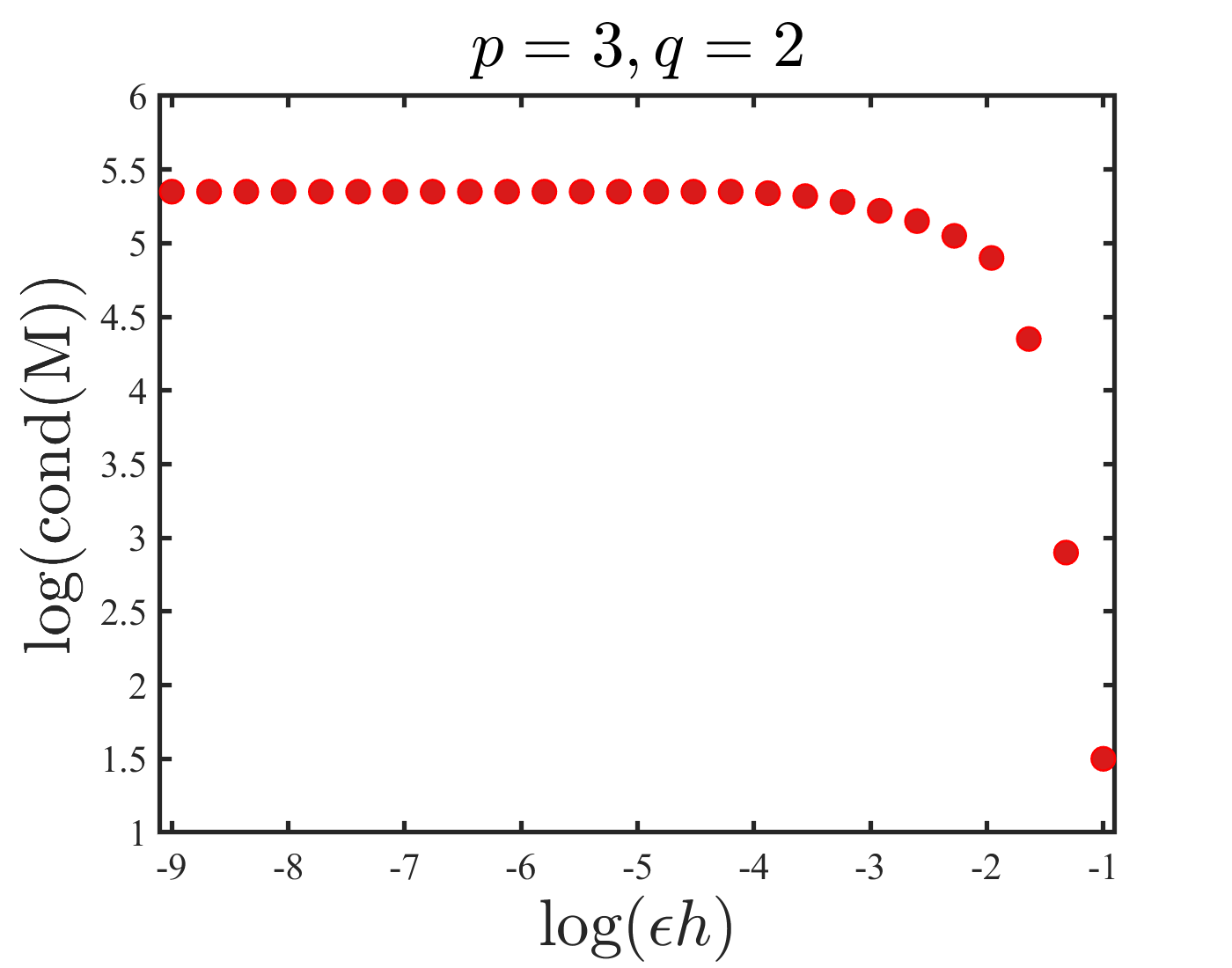
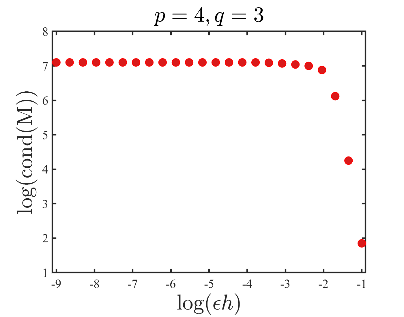
Figure 5.4 shows the condition number of the mass matrix and the maximum absolute value of the eigenvalues of the semi-discrete system matrix for a fixed number of cells, $N=20$ , with polynomial degrees $p=2,3,4,5$ and $q=p-1$ , respectively. To investigate their dependence on the cut-cell size, we set $\epsilon=10^{-m}$ , where $\epsilon=\eta$ defined in (2.17), and uniformly sample 30 values of $m$ over the interval $[0,6]$ . The numerical results demonstrate that the condition number of the mass matrix remains uniformly bounded with respect to the cut-cell configuration, and does not deteriorate as the volume fraction of the cut cells tends to zero, providing concrete evidence for the effectiveness of our proposed strategy. Moreover, the maximum absolute eigenvalue of the semi-discrete operator remains uniformly bounded as $\epsilon$ decreases, indicating that the proposed method effectively avoids the severe time-step restriction induced by arbitrarily small cut cells.

Remark 5.1.

All numerical simulations are implemented with alternating flux with $\alpha=\beta=\tau=0$ in (2.7), we can observe the optimal convergence rate $p+1$ . Furthermore, we also conduct numerical experiments using Sommerfeld flux ( $\alpha=\frac{1}{2},\beta=\tau=\frac{1}{2}$ ) and central flux ( $\alpha=\frac{1}{2},\beta=\tau=0$ ), and the resulting convergence rates remain consistent with those of the original EDG method [3].

Refer to caption — Figure 5.3: Example 5.1: $L^{2}$ errors of the CutEDG scheme at $t=0.8$ with different cut‑cell ratios $\epsilon$ and polynomial degrees $(p,q)$ .

Example 5.2.

Accuracy test for two dimensional problem

We now consider the two-dimensional wave equation

u_{tt}=u_{xx}+u_{yy},

(5.62)

In this example, two different domains are considered:

•

Rectangular domain $\Omega=[-\pi,\pi]^{2}$ , and the initial conditions and boundary conditions are given such that the exact solution is $u(x,y,t)=\sin(x)\sin(y)\cos(\sqrt{2}t)$ . Small cut elements exist in both $x$ - and $y$ -directions. The corresponding mesh configuration is illustrated in Figure 5.5. And parameters $\epsilon_{x}$ and $\epsilon_{y}$ are utilized to evaluate the relative cut-cell sizes in the $x$ - and $y$ -directions, respectively, see Figure 5(a).
•

A circular domain $\Omega=\{(x,y):x^{2}+y^{2}\leq 1\}$ , and initial conditions and homogeneous Dirichlet boundary are imposed to match the exact solution $u(x,y,t)=J_{0}\left(\alpha_{3}\sqrt{x^{2}+y^{2}}\right)\cos(\alpha_{3}t)$ , where, $J_{0}$ is the zeroth-order Bessel function of the first kind, and $\alpha_{n}$ denote its $n$ -th positive zero. The fictitious domain is chosen as $\Omega^{\prime}=[-1.1,1.1]^{2}$ , which is discretized by a uniform Cartesian background mesh, as illustrated in Figure 5(b)

For both cases, we set the final time $t=0.25$ and consider the polynomial degree $p=2,3,4$ , $q=p-1$ .

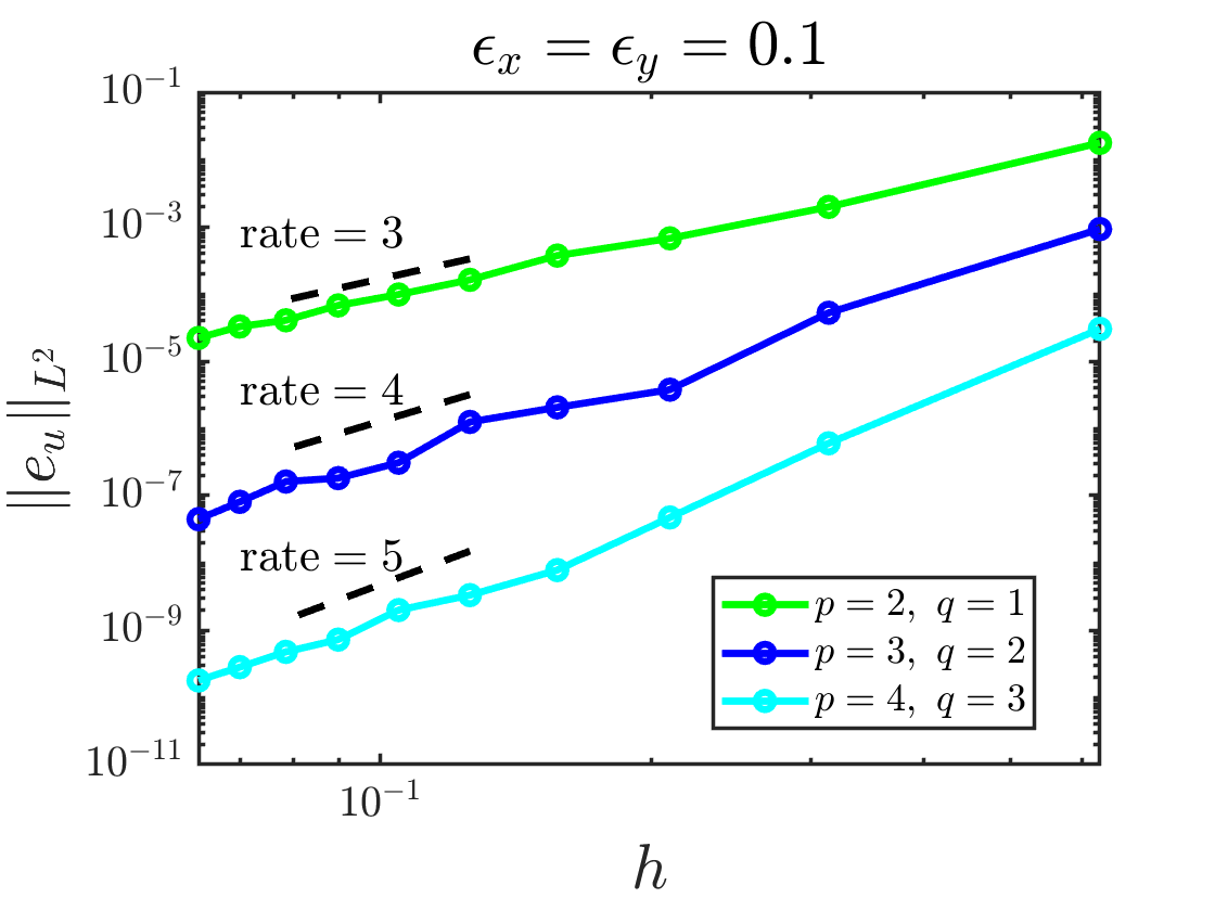
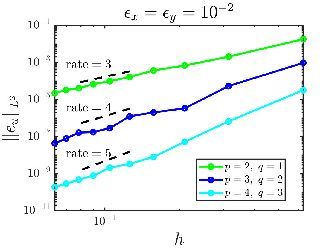
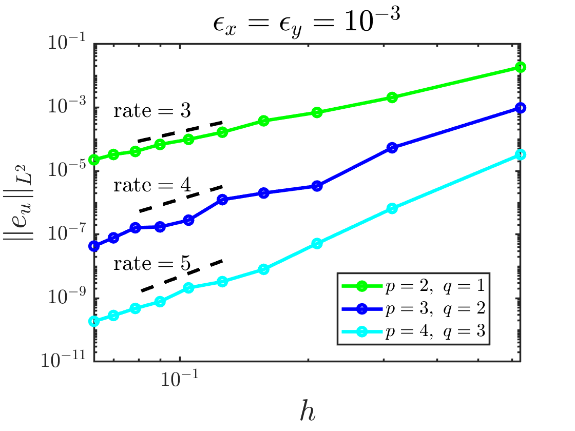
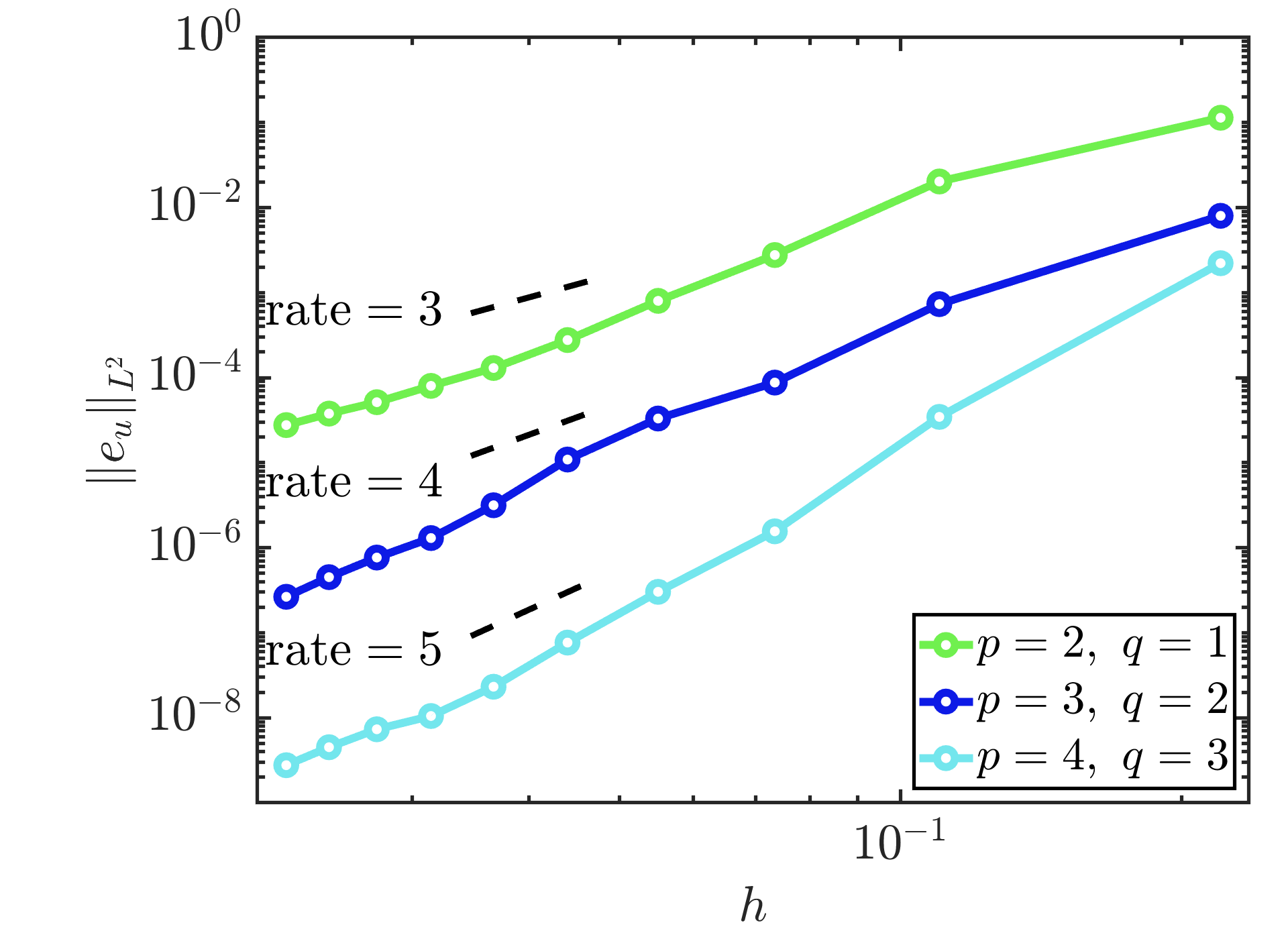
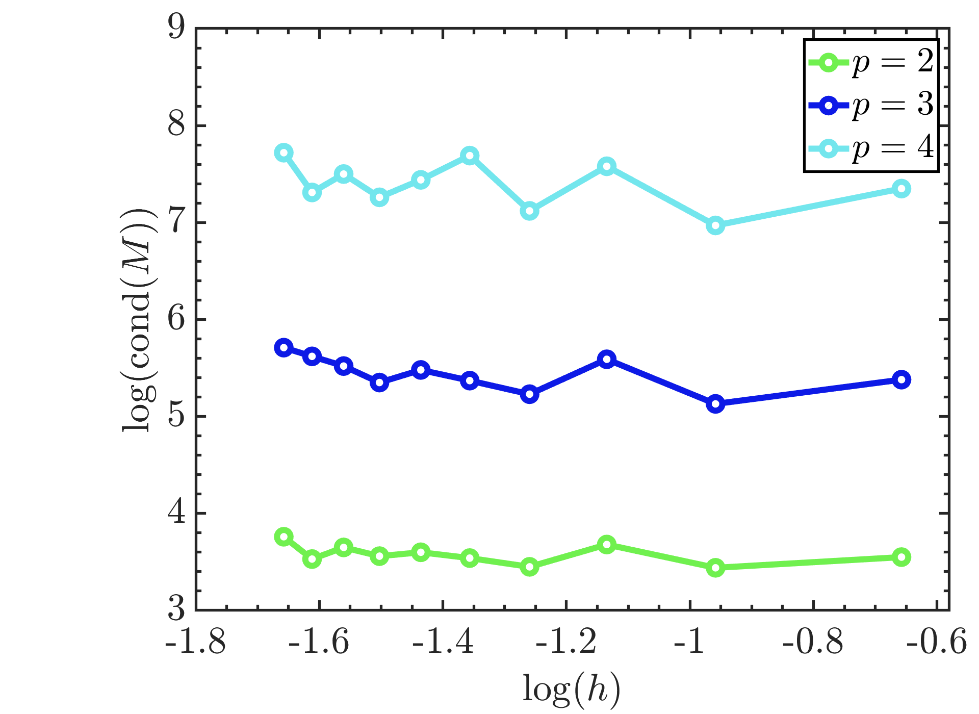
In Figure 5.6 and 5.7, we show the $L^{2}$ error of $u_{h}$ on rectangular domain and circle domain, respectively. Those numerical results demonstrate that the proposed CutEDG scheme can achieve the optimal order $p+1$ in both cases, further confirming its robustness and effectiveness. Figure 5.7 reports the condition numbers of the mass matrix for different polynomial degrees. The condition numbers of the proposed CutEDG scheme remain of the same order of magnitude as those of the high-order continuous CutFEM [26], with slightly smaller values for the polynomial degrees considered here. This indicates that the stabilization incorporated into the CutEDG formulation effectively controls the ill-conditioning associated with the cut cells, while maintaining a condition number comparable to that of the corresponding high-order CutFEM discretization. Nevertheless, the condition number still increases with the polynomial degree $p$ , indicating that the dependence of the mass-matrix conditioning on the polynomial degree persists.

Example 5.3.

Wave propagation around a triangular obstacle

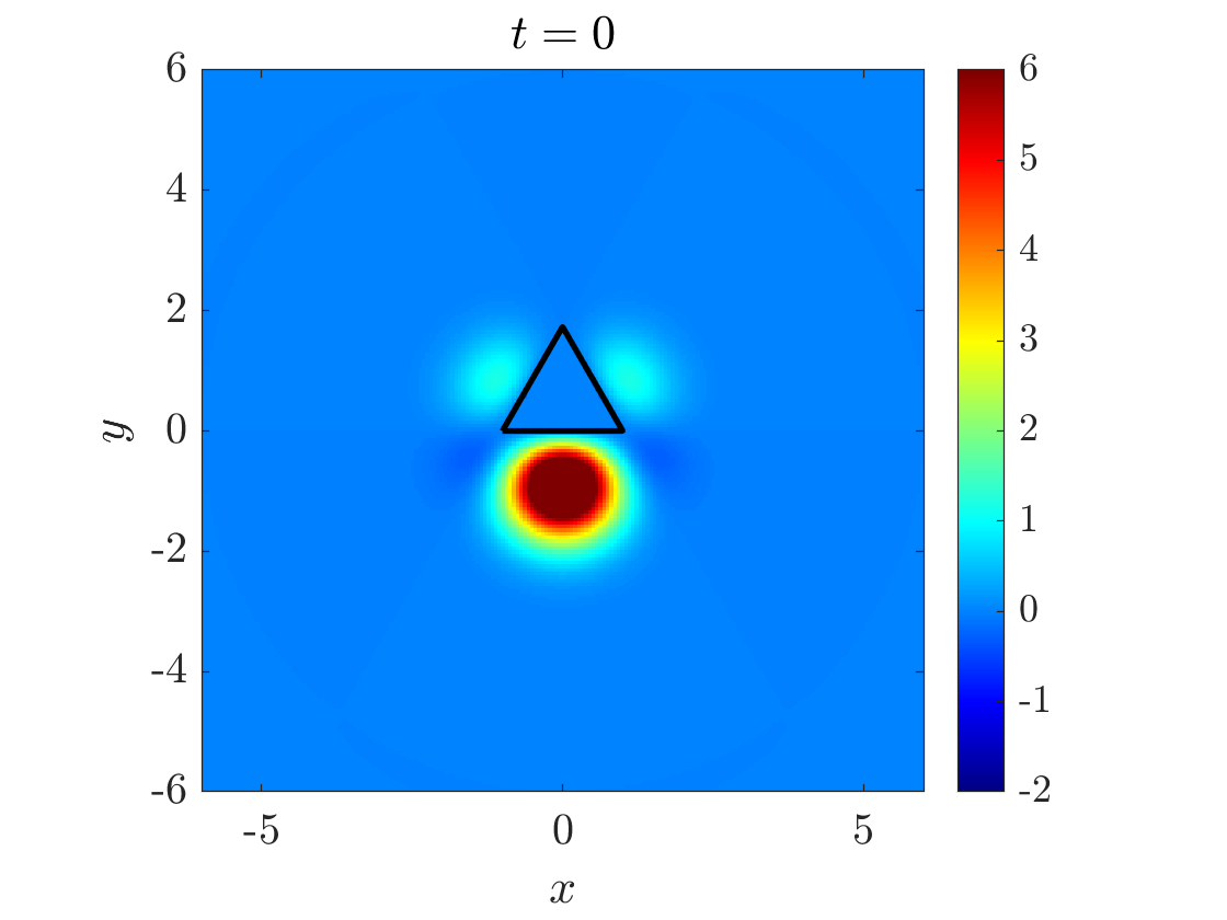
We consider the wave equation (5.62) on the computational domain $\Omega=[-6,6]^{2}$ with a triangular hole whose vertices are $(-1,0),(1,0),$ and $(0,\sqrt{3})$ . Homogeneous Dirichlet boundary conditions are enforced along the boundary of the domain both internal boundary and outer boundary. The initial conditions are chosen as

u|_{t=0}=\dfrac{1}{10}y(36-x^{2}-y^{2})(\sqrt{3}x-y+\sqrt{3})(\sqrt{3}x+y-\sqrt{3})e^{-(x^{2}+y^{2})},\quad u_{t}|_{t=0}=0.

We adopt Cartesian grids for spatial discretization, and the corresponding mesh partition schematic is illustrated in Figure 5.8. We choose $p=2$ and $q=1$ in the numerical simulation and the numerical solutions are computed at $t=0$ , $0.2$ , $0.5$ , and $0.8$ . As shown in Figure 5.9, the numerical solutions exhibit clear convergence as mesh refined, demonstrating the robustness of the proposed method for wave propagation in domains with non-grid-aligned boundaries.

Example 5.4.

An Immersed Outer Problem

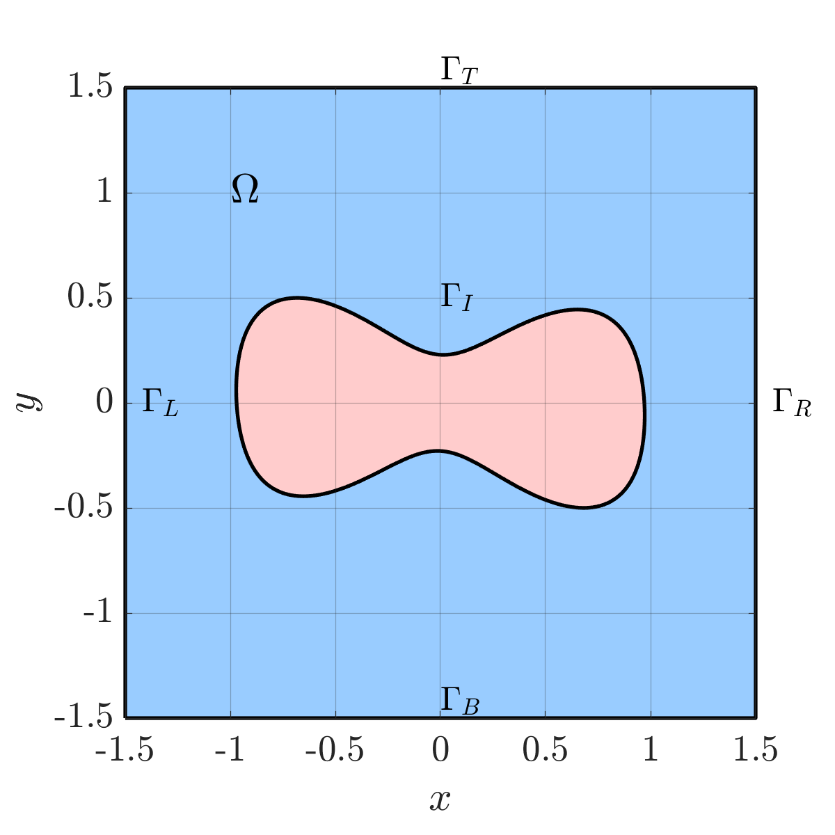
We further consider an exterior problem whose geometry is illustrated in Figure 5.10. The interior boundary is given by the zero level set of the function

\phi(x,y)=-\left(s^{4}(x^{4}+y^{4})+\dfrac{1}{4}s^{2}xy-2s^{2}x^{2}+2s^{2}y^{2}-\frac{1}{4}\right)

where $s=1.5$ . The computational domain $\Omega$ is defined as

\Omega=\{(x,y)\in\mathbb{R}^{2}:x,y\in(-1.5,1.5):\phi(x,y)<0\}.

(5.63)

The initial conditions are homogeneous with $u|_{t=0}=0,u_{t}|_{t=0}=0$ . A homogeneous Neumann boundary condition, $\dfrac{\partial u}{\partial\mathbf{n}}|_{\Gamma_{I}}=0$ , is imposed on the internal boundary $\Gamma_{I}$ . where $\mathbf{n}$ denotes the unit outward normal to $\Gamma_{I}$ . On the external boundaries, Dirichlet conditions are prescribed:

u=\begin{cases}g_{D}(x,t),&x\in\Gamma_{B},\\ 0,&x\in\Gamma_{L}\cup\Gamma_{R}\cup\Gamma_{U},\end{cases}

where $g_{D}$ is given by

g_{D}(x,t)=\cos\left(\frac{\pi}{3}x\right)e^{-(t-t_{c})^{2}/\sigma^{2}},\qquad\sigma=0.25,t_{c}=3.

Several snapshots of the numerical solution are presented in Figure 5.11. As an explicit exact solution is not available for the present test case, the numerical solution on a sufficiently refined mesh is taken as the reference solution for assessing the discretization error and convergence order. As shown in Figure 5.12, we compute the numerical errors corresponding to mesh resolutions of 8 $\times$ 8, 16 $\times$ 16, 32 $\times$ 32, 64 $\times$ 64, and 128 $\times$ 128 respectively. It is observed that the numerical solution remains convergent, and the computed convergence rates achieve the optimal orders.

Example 5.5.

Interface Problem

Finally, we consider the following initial-boundary-value problem for the wave equation on a partitioned domain:

\begin{cases}u_{tt}-c_{1}^{2}\Delta u=0,&(x,y)\in\mathbb{R}_{L}^{2},\quad t>0,\\ v_{tt}-c_{2}^{2}\Delta v=0,&(x,y)\in\mathbb{R}_{R}^{2},\quad t>0,\\ u-v=0,&x=0,\quad t>0,\\ c_{1}^{2}u_{x}-c_{2}^{2}v_{x}=0,&x=0,\quad t>0.\end{cases}

where $\mathbb{R}_{L}^{2}=\{(x,y):x<0\}$ and $\mathbb{R}_{R}^{2}=\{(x,y):x>0\}$ denote the left and right half-planes, respectively. The interface conditions at $x=0$ enforce continuity of the solution and conservation of the normal flux, which model transmission and reflection across the material interface. The exact solution to this problem is given by

\begin{cases}u=\cos(x+y-\sqrt{2}c_{1}t)+k_{2}\cos(x-y+\sqrt{2}c_{1}t),\\ v=(1+k_{2})\cos(k_{1}x+y-\sqrt{2}c_{1}t),\end{cases}

with the parameters

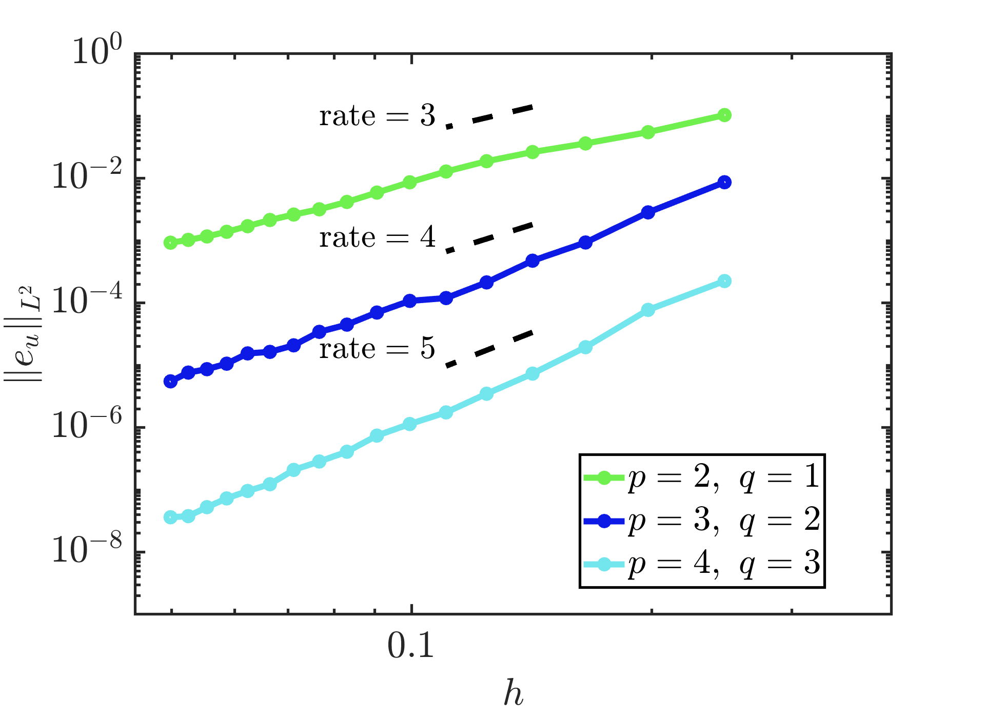
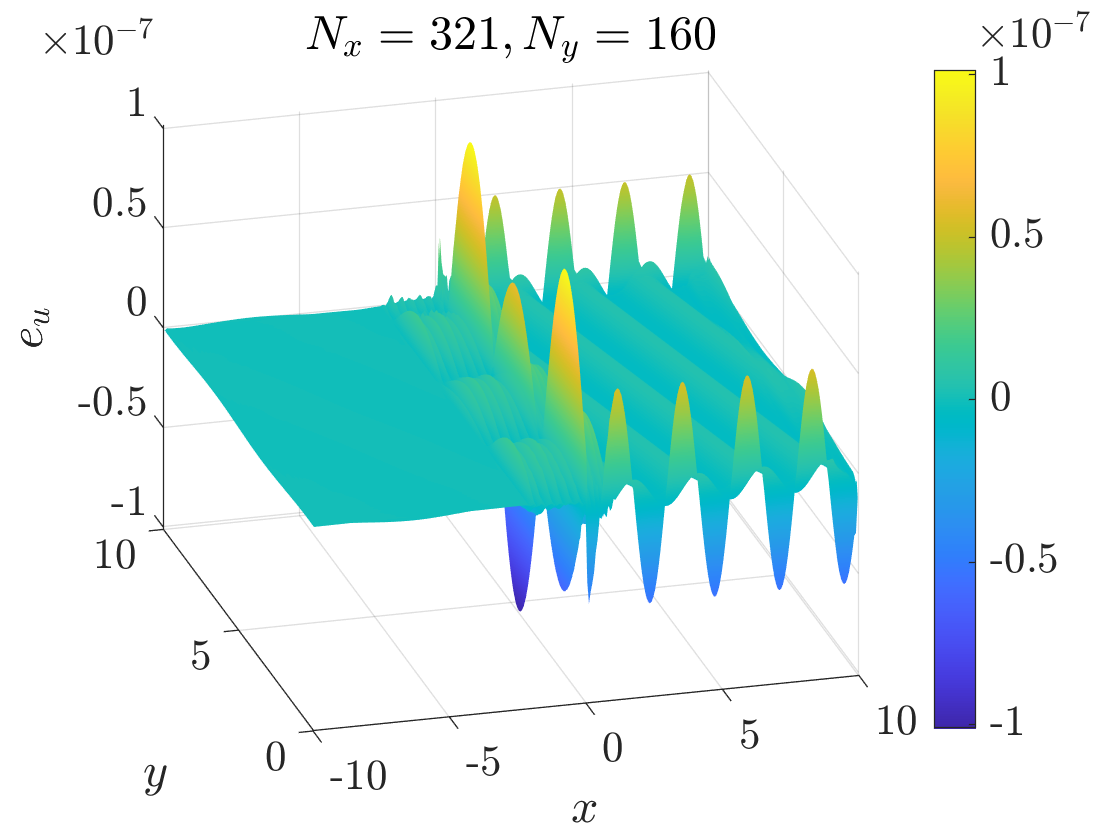
k_{1}=\sqrt{\dfrac{2c_{1}^{2}}{c_{2}^{2}}-1},\qquad k_{2}=\dfrac{c_{1}^{2}-c_{2}^{2}k_{1}}{c_{1}^{2}+c_{2}^{2}k_{1}}.

In our numerical experiments, we set $c_{1}=1$ and $c_{2}=0.5$ . This choice makes the wavenumber in the right half plane twice as large as that in the left half plane, which can be seen in the plot of the exact solution at time $t=0$ in Figure 5.13. We restrict the domain to $[-10,10]\times[0,10]$ , impose Dirichlet boundary conditions at all outer boundaries, and use the exact solution to obtain the initial and boundary data. As shown in Figure 5.15, it is observed that the numerical solutions approach the exact solution monotonically as the mesh is refined, confirming the convergence of our method. Figure 5.14 reports the errors and convergence orders obtained with various polynomial spaces at the final time $t=2$ . The results again demonstrate that the scheme achieves the optimal convergence rate predicted by theory.

6 Conclusion

In this work, we developed a high-order CutEDG method for acoustic wave equations on unfitted meshes. By introducing ghost-penalty stabilization directly into the local bilinear forms defining the discrete EDG energy, the method retains the original flux structure while restoring robustness with respect to arbitrarily small cut cells. We established semidiscrete energy stability and high-order error estimates, and extended the formulation to stationary interface problems with discontinuous wave speeds. Numerical experiments confirmed the expected convergence rates, cut-independent conditioning, and an explicit time-step restriction governed by the background mesh size rather than the smallest physical cut cell. These results demonstrate the potential of CutEDG as a robust and accurate framework for high-order wave propagation in geometrically complex media.

References

[1] M. Ainsworth (2004) Discrete dispersion relation for hp-version finite element approximation at high wave number. SIAM Journal on Numerical Analysis 42 (2), pp. 553–575. Cited by: §1.
[2] D. Appelö, T. Hagstrom, Q. Wang, and L. Zhang (2020) An energy-based discontinuous Galerkin method for semilinear wave equations. Journal of Computational Physics 418, pp. 109608. Cited by: §1.
[3] D. Appelö and T. Hagstrom (2015) A new discontinuous Galerkin formulation for wave equations in second-order form. SIAM Journal on Numerical Analysis 53 (6), pp. 2705–2726. External Links: Document Cited by: §1, §2.1, §2, §3.2, Remark 3.1, Remark 5.1.
[4] D. Appelö and T. Hagstrom (2018) An energy-based discontinuous Galerkin discretization of the elastic wave equation in second order form. Computer Methods in Applied Mechanics and Engineering 338, pp. 362–391. Cited by: §1.
[5] P. Bastian and C. Engwer (2009) An unfitted finite element method using discontinuous Galerkin. International journal for numerical methods in engineering 79 (12), pp. 1557–1576. Cited by: §1.
[6] E. Burman, S. Claus, P. Hansbo, M. G. Larson, and A. Massing (2015) CutFEM: discretizing geometry and partial differential equations. International journal for numerical methods in engineering 104 (7), pp. 472–501. Cited by: §1, §1.
[7] E. Burman and P. Hansbo (2012) Fictitious domain finite element methods using cut elements: II. A stabilized Nitsche method. Applied Numerical Mathematics 62 (4), pp. 328–341. Cited by: §1, §1.
[8] E. Burman (2010) Ghost penalty. Comptes Rendus Mathematique 348 (21-22), pp. 1217–1220. External Links: Document Cited by: §1.
[9] P. Fu, T. Frachon, G. Kreiss, and S. Zahedi (2022) High order discontinuous cut finite element methods for linear hyperbolic conservation laws with an interface. Journal of Scientific Computing 90 (3), pp. 84. Cited by: §1.
[10] P. Fu, G. Kreiss, and S. Zahedi (2024) A bound preserving cut discontinuous Galerkin method for one dimensional hyperbolic conservation laws. ESAIM: Mathematical Modelling and Numerical Analysis 58 (5), pp. 1651–1680. Cited by: §1.
[11] P. Fu and G. Kreiss (2021) High order cut discontinuous Galerkin methods for hyperbolic conservation laws in one space dimension. SIAM Journal on Scientific Computing 43 (4), pp. A2404–A2424. Cited by: §1.
[12] M. J. Grote, A. Schneebeli, and D. Schötzau (2006) Discontinuous Galerkin finite element method for the wave equation. SIAM Journal on Numerical Analysis 44 (6), pp. 2408–2431. Cited by: §1.
[13] C. Gürkan and A. Massing (2019) A stabilized cut discontinuous Galerkin framework for elliptic boundary value and interface problems. Computer Methods in Applied Mechanics and Engineering 348, pp. 466–499. External Links: Document Cited by: §1.
[14] C. Gürkan, S. Sticko, and A. Massing (2020) Stabilized cut discontinuous Galerkin methods for advection-reaction problems. SIAM Journal on Scientific Computing 42 (5), pp. A2620–A2654. External Links: Document Cited by: §1.
[15] J. S. Hesthaven and T. Warburton (2008) Nodal discontinuous Galerkin methods: algorithms, analysis, and applications. Springer. Cited by: §1.
[16] F. Ihlenburg (1998) Finite element analysis of acoustic scattering. Springer. Cited by: §1.
[17] E. L. Kawecki (2020) Finite element theory on curved domains with applications to discontinuous Galerkin finite element methods. Numerical Methods for Partial Differential Equations 36 (6), pp. 1492–1536. Cited by: §1.
[18] D. Komatitsch and J. Tromp (1999) Introduction to the spectral element method for three-dimensional seismic wave propagation. Geophysical journal international 139 (3), pp. 806–822. Cited by: §1.
[19] B. Müller, S. Krämer-Eis, F. Kummer, and M. Oberlack (2017) A high-order discontinuous Galerkin method for compressible flows with immersed boundaries. International Journal for Numerical Methods in Engineering 110 (1), pp. 3–30. External Links: Document Cited by: §1.
[20] R. Qin and L. Krivodonova (2013) A discontinuous Galerkin method for solutions of the Euler equations on Cartesian grids with embedded geometries. Journal of Computational Science 4 (1-2), pp. 24–35. External Links: Document Cited by: §1.
[21] K. Ren, L. Zhang, and Y. Zhou (2024) An energy-based discontinuous Galerkin method for the nonlinear schrödinger equation with wave operator. SIAM Journal on Numerical Analysis 62 (6), pp. 2459–2483. Cited by: §1.
[22] L. W. Schmerr (2016) Fundamentals of ultrasonic nondestructive evaluation. Vol. 122, Springer. Cited by: §1.
[23] R. Sevilla, S. Fernández-Méndez, and A. Huerta (2011) Comparison of high-order curved finite elements. International Journal for Numerical Methods in Engineering 87 (8), pp. 719–734. Cited by: §1.
[24] P. Shukla and J. van der Vegt (2022) A space-time interior penalty discontinuous Galerkin method for the wave equation. Communications on Applied Mathematics and Computation 4 (3), pp. 904–944. Cited by: §1.
[25] S. Sticko and G. Kreiss (2016) A stabilized Nitsche cut element method for the wave equation. Computer methods in applied mechanics and engineering 309, pp. 364–387. Cited by: §1.
[26] S. Sticko and G. Kreiss (2019) Higher order cut finite elements for the wave equation. Journal of Scientific Computing 80 (3), pp. 1867–1887. Cited by: §1, §2.4, §5.
[27] I. Weber and G. Kreiss (2026) A fourth order cut finite element (cutfem) method for the wave equation using the modified equation approach. Journal of Scientific Computing 109, pp. 10. External Links: Document Cited by: §1.
[28] Y. Xing, C. Chou, and C. Shu (2013) ENERGY conserving local discontinuous Galerkin methods for wave propagation problems.. Inverse Problems & Imaging 7 (3). Cited by: §1.
[29] L. Zhang, T. Hagstrom, and D. Appelo (2019) An energy-based discontinuous Galerkin method for the wave equation with advection. SIAM Journal on Numerical Analysis 57 (5), pp. 2469–2492. Cited by: §1.
[30] X. Zhang (2016) A curved boundary treatment for discontinuous Galerkin schemes solving time dependent problems. Journal of Computational Physics 308, pp. 153–170. Cited by: §1.

	$\displaystyle\\|\nabla(u-u_{h})\\|_{L^{2}(\Omega)}^{2}+\\|v-v_{h}\\|_{L^{2}(\Omega)}^{2}\lesssim$	$\displaystyle h^{2\gamma}\left(\|u\|_{H^{p+1}(\Omega)}^{2}+\|v\|_{H^{q+1}(\Omega)}^{2}\right)$		(3.29)
		$\displaystyle+h^{2p}\|u_{t}\|_{H^{p+1}(\Omega)}^{2}+h^{2(q+1)}\|v_{t}\|_{H^{q+1}(\Omega)}^{2},$		(3.29)

	$\displaystyle\dfrac{1}{2}\dfrac{d}{dt}\left(\sum_{K}\int_{K_{\Omega}}\|\nabla\tilde{e}_{u}\|^{2}+\tilde{e}_{v}^{2}\,d\mathbf{x}+\gamma_{M}^{(u)}h^{-2}J(\tilde{e}_{u},\tilde{e}_{u})+\gamma_{M}^{(v)}J(\tilde{e}_{v},\tilde{e}_{v})\right)$	(3.40)
$\displaystyle\lesssim$	$\displaystyle\sum_{K}\int_{K_{\Omega}}\|\nabla\tilde{e}_{u}\|^{2}+\tilde{e}_{v}^{2}\,d\mathbf{x}+\gamma_{M}^{(u)}h^{-2}J(\tilde{e}_{u},\tilde{e}_{u})+\gamma_{M}^{(v)}J(\tilde{e}_{v},\tilde{e}_{v})$
	$\displaystyle+h^{2\gamma}\left(\|u\|^{2}_{H^{p+1}(\Omega)}+\|v\|^{2}_{H^{q+1}(\Omega)}\right)+h^{2p}\|u_{t}\|^{2}_{H^{p+1}(\Omega)}+h^{2(q+1)}\|v_{t}\|^{2}_{H^{q+1}(\Omega)}.$