跳到论文正文
W Papers独立论文阅读器 arXiv:2609.38141 论文正文 计算阅读时间 · 0%
引用这篇论文根据当前论文元数据生成,正式投稿前建议核对。


License: arXiv.org perpetual non-exclusive license
arXiv:2609.38141v1 [stat.ME] 29 Sep 2026

Global Synchronization for Multi-Source Data Integration under Blockwise Missing Patterns

Runbing Zheng ††thanks: Email: runbing@stanford.edu. Affiliation: Department of Neurology and Neurological Sciences, Stanford University    Dmitriy Kunisky ††thanks: Email: kunisky@jhu.edu. Affiliation: Department of Applied Mathematics & Statistics, Johns Hopkins University
September 29, 2026
Abstract

Multi-source data integration problems over datasets from different sources covering different but possibly overlapping sets of entities have become increasingly important in many real-world areas, including genomics, single-cell analysis, and healthcare research. In such problems, one often first learns a low-dimensional representation of the entities within each source and then integrates these representations across sources. As the representations from different sources are only identifiable up to some transformation, how to align them across sources using the sources’ overlapping entities becomes a key challenge. Existing methods align the sources in a sequential or tree-structured manner, and are therefore sensitive to the chosen order and exploit only part of the available overlapping information. Motivated by this limitation, we propose Global Synchronized Multiple Matrix Integration (GSMMI), which formulates this alignment problem as a global synchronization problem and jointly aligns all sources using all pairwise overlaps at once, thereby making full use of all overlapping information across the sources. We develop an efficient iterative algorithm for GSMMI that is fast and scalable to the large-scale data arising in these applications. We show both theoretically and empirically that GSMMI improves alignment accuracy, with clear improvements even under modest overlap structure. Moreover, we develop GSMMI to be broadly applicable across data types, covering symmetric positive semidefinite, symmetric indefinite, and asymmetric or rectangular matrices, and even settings where sources overlap only in their rows or only in their columns, making it suitable for a wide variety of application scenarios.

Keywords: data integration, blockwise missing pattern, matrix completion, synchronization

1 Introduction

The rapid growth of large-scale data collection and sharing has made multi-source data integration an increasingly important problem in modern statistics, with applications ranging across healthcare research (Zhou et al., 2023), genomics (Maneck et al., 2011; Tseng et al., 2015; Zang et al., 2016; Cai et al., 2016), single-cell analysis (Stuart et al., 2019; Argelaguet et al., 2021; Ma et al., 2024), and chemometrics (Mishra et al., 2021).

A key feature of multi-source data integration is that it often gives rise to problems with missing blocks of data, where each source observes a submatrix of the entire underlying data matrix, with different sources covering different but potentially overlapping subsets of its rows and columns. We give three motivating examples here to illustrate how differences in coverage across sources give rise to distinct forms of block-wise missing data.

First, consider pointwise mutual information (PMI) matrices derived from electronic health record (EHR) data. PMI measures associations between pairs of clinical concepts based on their co-occurrence (Ahuja et al., 2020; Zhou et al., 2022). Because healthcare systems have limited interoperability (Rajkomar et al., 2018), different EHR datasets often cover partially overlapping sets of concepts. Each PMI matrix therefore provides a square block of the full concept-by-concept matrix, with shared concepts giving rise to overlapping blocks, as shown in Figure 1(a). Second, in single-cell data, each dataset records measurements of genomic features across cells. Experiments spanning different batches, tissues, or technologies may cover different, potentially overlapping sets of cells and features (Ma et al., 2020; Lähnemann et al., 2020). The resulting matrices provide rectangular blocks that may overlap along both dimensions, as illustrated in Figure 1(b). Third, in multimodal health data, different modalities measure distinct sets of features, but not every subject has data available for every modality, for reasons such as cost. The resulting matrices have disjoint feature sets and partially overlapping subject sets, producing the pattern in Figure 1(c).

(a) PMI matrices

(b) Single-cell matrices

(c) Multimodal health data

Figure 1: Block-wise observation patterns in three multi-source integration settings: (a) PMI matrices from different EHR systems, (b) single-cell matrices from different experiments, and (c) multimodal health data. Different colors indicate blocks observed by different sources, and blended colors indicate overlaps between sources.

As illustrated in Figure 1, in all of these cases, integrating the observations from different sources can involve a structured, block-wise missing pattern, rather than the uniformly or independently sampled entries that are commonly assumed in the matrix completion literature. Thus, although there is a rich body of literature on matrix completion (see, e.g., Candes and Recht (2012); Candes and Plan (2011); Koltchinskii et al. (2011); Chen et al. (2019); Fornasier et al. (2011); Mohan and Fazel (2012); Vandereycken (2013); Hu et al. (2012); Chen et al. (2020); Cai and Zhou (2016); Foygel et al. (2011) for some of the key references), most of these methods are not well-suited to the multi-source data integration problem considered here, since they mainly focus on recovering a possibly low-rank matrix under the assumption of uniformly or independently sampled observed entries.

For block-wise missing data, much existing work is developed for particular tasks under specialized assumptions. For instance, Xue and Qu (2021); Xue et al. (2021); He et al. (2023); Zhang et al. (2020) study regression problems in which the design matrix has block-wise missing entries. Specifially, Xue and Qu (2021) propose a multiple block-wise imputation approach for model selection under a linear model; Xue et al. (2021) develop debiased estimators and valid confidence intervals for high-dimensional linear regression based on unbiased estimating equations and block-wise imputation; He et al. (2023) develop a single regression-based imputation algorithm, built on sparse precision matrix estimation, for variable selection under a generalized linear model; and Zhang et al. (2020) propose a factor-model imputation approach that yields an imputed factor regression for dimension reduction and prediction. Beyond regression, Sui et al. (2026) propose a multi-task learning framework that imputes the missing blocks via shared and task-specific representations to predict a target of interest for each task. Wang et al. (2026) study multimodal domain adaptation under a label-shift assumption, using labeled source datasets with block-wise missing modalities to predict outcomes in an unlabeled target population. Zhu et al. (2020) propose a generalized integrative principal component analysis procedure, which assumes the data sources share common samples but distinct variables, and models each source with a possibly different exponential-family distribution.

Further, some work on multi-source data integration under block-wise missing patterns (Zhou et al., 2023; Bishop and Yu, 2014; Zheng et al., 2026; Liu et al., 2026; Zheng and Tang, 2026) does not target a specific downstream task or rely on associated specialized assumptions, but instead aims to recover the full low-rank matrix, or equivalently the latent positions of all entities in a low-dimensional space, which is the problem we consider in this paper. This is typically achieved in two steps: one first applies a low-rank estimation method, such as a spectral method, to each source to estimate the latent positions of the entities it observes. Because the latent positions estimated from different sources are only identifiable up to some transformation and can therefore differ across sources, one then aligns them using the entities shared between overlapping sources.

Existing methods differ mainly in how the alignment in the second step is performed. Zhou et al. (2023) align each pair of overlapping submatrices on their shared entities to match their latent positions and then recovers the entries associated with that pair. Since this alignment is carried out in a pairwise manner and does not produce a globally consistent representation across all sources, the portion of the matrix that ends up recovered correctly may be limited. Bishop and Yu (2014) focus on symmetric positive semidefinite matrices and integrate all the submatrices sequentially, aligning the latent positions of each new submatrix to the entities already covered by the previously integrated submatrices. Such a sequential procedure can yield globally aligned latent positions for all entities covered by the integrated submatrices, but it is restrictive as a way of aligning the sources, and its performance is sensitive to the integration order, yet how to determine an effective order remains unresolved in Bishop and Yu (2014). Moreover, because the alignment is propagated in a one-directional, sequential manner and once-fixed alignments are never corrected by later overlaps, the sequential procedure does not fully exploit all of the available overlapping information. Zheng et al. (2026) studies rectangular data and likewise aligns the submatrices sequentially, and additionally provides a greedy algorithm for ordering them. Liu et al. (2026) also focuses on rectangular data and aligns the sources through a set of anchor features shared across all sources, and then the alignment relies solely on the overlap over this anchor block, which may constitute only a small fraction of all the available overlapping information. And when such a globally shared feature set does not exist, Liu et al. (2026) proceeds by sequentially linking overlapping groups one after another, where each group is first estimated using its own shared features and successive groups are then aligned through their overlapping members, along a prespecified order. It provides no algorithm to determine the order, and this sequential linking method again involves limitations similar to those of the sequential procedures noted above. Zheng and Tang (2026) proposes the chain-linked multiple matrix integration (CMMI) method. Rather than relying on a sequential order, CMMI encodes the overlaps among sources as a graph, whose vertices represent the observed submatrices and whose edges represent overlapping pairs, and then selects a spanning tree of this graph to align all submatrices along a common coordinate system, yielding a globally consistent alignment. It further provides a method for choosing a favorable spanning tree that can lead to smaller alignment error. By breaking free from the restriction of sequential integration, CMMI makes it possible to align the sources in a better way. Nevertheless, like all the methods above that aim at globally aligned latent positions, CMMI still does not fully utilize all available overlapping information, as it uses only the overlaps along the chosen spanning tree. These limitations motivate an alignment scheme that exploits the entire structure of overlapping observations.

In this paper, building on CMMI, we propose Global Synchronized Multiple Matrix Integration (GSMMI), which aligns all sources by exploiting all pairwise overlaps rather than only a subset of them. Specifically, we formulate the alignment as a global synchronization problem, jointly seeking transformations for all sources that simultaneously match the latent positions of every pair of overlapping submatrices over all of their shared entities. Unlike CMMI and the other methods above, which propagate alignments along a sequence or a spanning tree and thus rely on only part of the overlapping information, GSMMI aggregates the alignment information from all overlapping pairs at once, thereby making full use of the overlapping structure. Computational efficiency is another important consideration for multi-source data integration, since applications in areas such as genomics, single-cell analysis, and healthcare research often involve large-scale data. A notable advantage of CMMI is that its alignment mainly involves a sequence of singular value decompositions and is therefore computationally very fast. To preserve this efficiency, we develop an iterative algorithm for the global synchronization problem, in which each update reduces to a Procrustes or least-squares subproblem that admits an efficient closed-form solution. We further use the CMMI solution as a high-quality initialization, which empirically allows GSMMI to converge accurately and rapidly, so that its running time is close to, or at most a few times, that of CMMI.

The structure of our paper is as follows. In Section 2, we introduce the model for multiple observed submatrices of a whole symmetric positive semidefinite matrix, revisit the CMMI algorithm, and then present the proposed GSMMI algorithm. In Section 3, we provide a theoretical analysis showing that GSMMI can achieve improved alignment accuracy over CMMI, particularly when the number of sources is large and the overlapping structure is rich. Numerical simulations and real-data experiments are presented in Sections 4 and 5, illustrating that GSMMI outperforms CMMI in estimation accuracy while incurring only a modest computational overhead. Finally, although the main idea and analysis of GSMMI are presented for the case of symmetric positive semidefinite matrices for simplicity, GSMMI can be extended to symmetric indefinite matrices as well as asymmetric or rectangular matrices, as we show in Section 6, so that it is applicable to the full range of multiple matrix integration problems, including all the settings illustrated in Figure 1.

1.1 Notation

We summarize some notations used in this paper. For any positive integer nn, we denote by [n][n] the set {1,2,…,n}\{1,2,\dots,n\}.

Asymptotics

For two non-negative sequences {an}n≥1\{a_{n}\}_{n\geq 1} and {bn}n≥1\{b_{n}\}_{n\geq 1}, we write an≲bna_{n}\lesssim b_{n} (resp. an≳bna_{n}\gtrsim b_{n}) if there exists some constant C>0C>0 such that an≤C​bna_{n}\leq Cb_{n} (resp. an≥C​bna_{n}\geq Cb_{n}) for all n≥1n\geq 1, and we write an≍bna_{n}\asymp b_{n} if an≲bna_{n}\lesssim b_{n} and an≳bna_{n}\gtrsim b_{n}. If an/bna_{n}/b_{n} stays bounded away from +∞+\infty, we write an=O⁡(bn)a_{n}=O(b_{n}) and bn=Ω⁡(an)b_{n}=\Omega(a_{n}), and we use the notation an=Θ⁡(bn)a_{n}=\Theta(b_{n}) to indicate that an=O⁡(bn)a_{n}=O(b_{n}) and an=Ω⁡(bn)a_{n}=\Omega(b_{n}). If an/bn→0a_{n}/b_{n}\to 0, we write an=o⁡(bn)a_{n}=o(b_{n}) and bn=ω⁡(an)b_{n}=\omega(a_{n}). We say a sequence of events 𝒜n\mathcal{A}_{n} holds with high probability if for any c>0c>0 there exists a finite constant n0n_{0} depending only on cc such that ℙ⁡(𝒜n)≥1−n−c\mathbb{P}(\mathcal{A}_{n})\geq 1-n^{-c} for all n≥n0n\geq n_{0}. We write an=Op​(bn)a_{n}=O_{p}(b_{n}) (resp. an=op​(bn)a_{n}=o_{p}(b_{n})) to denote that an=O⁡(bn)a_{n}=O(b_{n}) (resp. an=o⁡(bn)a_{n}=o(b_{n})) holds with high probability.

Linear algebra

We denote by 𝒪d\mathcal{O}_{d} the set of d×dd\times d orthogonal matrices, and let 𝒪n×d:={𝑼∈ℝn×d∣𝑼⊤​𝑼=𝑰d}\mathcal{O}_{n\times d}:=\{\bm{U}\in\mathbb{R}^{n\times d}\mid\bm{U}^{\top}\bm{U}=\bm{I}_{d}\}. For any matrix 𝑴∈ℝA×B\bm{M}\in\mathbb{R}^{A\times B} and index sets 𝒜⊆[A]\mathcal{A}\subseteq[A], ℬ⊆[B]\mathcal{B}\subseteq[B], we denote by 𝑴𝒜,ℬ∈ℝ|𝒜|×|ℬ|\bm{M}_{\mathcal{A},\mathcal{B}}\in\mathbb{R}^{|\mathcal{A}|\times|\mathcal{B}|} the submatrix of 𝑴\bm{M} formed from rows 𝒜\mathcal{A} and columns ℬ\mathcal{B}, and we denote by 𝑴𝒜∈ℝ|𝒜|×B\bm{M}_{\mathcal{A}}\in\mathbb{R}^{|\mathcal{A}|\times B} the submatrix of 𝑴\bm{M} consisting of the rows indexed by 𝒜\mathcal{A}. The Hadamard product between conformal matrices 𝑴\bm{M} and 𝑵\bm{N} is denoted by 𝑴∘𝑵\bm{M}\circ\bm{N}. Given a matrix 𝑴\bm{M}, we denote its spectral, Frobenius, and infinity norms by ‖𝑴‖\|\bm{M}\|, ‖𝑴‖F\|\bm{M}\|_{F}, and ‖𝑴‖∞\|\bm{M}\|_{\infty}. We also denote the 2→∞2\to\infty norm of 𝑴\bm{M} by ‖𝑴‖2→∞=max‖𝒙‖=1⁡‖𝑴​𝒙‖∞=maxi⁡‖𝒎i‖,\|\bm{M}\|_{2\to\infty}=\max_{\|\bm{x}\|=1}\|\bm{M}\bm{x}\|_{\infty}=\max_{i}\|\bm{m}_{i}\|, where 𝒎i\bm{m}_{i} denotes the iith row of 𝑴\bm{M}, i.e., ‖𝑴‖2→∞\|\bm{M}\|_{2\to\infty} is the maximum of the ℓ2\ell_{2} norms of the rows of 𝑴\bm{M}.

2 Methodology and Proposed Algorithm

We first formulate a precise model of data integration problems. Suppose we are interested in an unobserved low-rank population matrix 𝑷∈ℝN×N\bm{P}\in\mathbb{R}^{N\times N} associated with NN entities. For now, we further suppose 𝑷\bm{P} is positive semidefinite with rank d≪Nd\ll N; extensions to the case of symmetric but indefinite 𝑷\bm{P}, as well as asymmetric or rectangular 𝑷\bm{P}, including the corresponding algorithms, are presented in Section 6. Denote the eigendecomposition of 𝑷\bm{P} by 𝑷=𝑼​𝚲​𝑼⊤\bm{P}=\bm{U}\bm{\Lambda}\bm{U}^{\top}, where 𝚲∈ℝd×d\bm{\Lambda}\in\mathbb{R}^{d\times d} is a diagonal matrix whose diagonal entries are the non-zero eigenvalues of 𝑷\bm{P} in descending order, and the orthonormal columns of 𝑼∈𝒪N×d\bm{U}\in\mathcal{O}_{N\times d} are the corresponding eigenvectors. We define the latent positions of the entities as 𝑿=𝑼​𝚲1/2∈ℝN×d\bm{X}=\bm{U}\bm{\Lambda}^{1/2}\in\mathbb{R}^{N\times d}, where the ssth row 𝒙s\bm{x}_{s} gives the latent position of entity ss in ℝd\mathbb{R}^{d}. Then we have 𝑷=𝑿​𝑿⊤\bm{P}=\bm{X}\bm{X}^{\top}, and each entry is the inner product of the corresponding latent positions, i.e., 𝑷s,t=𝒙s⊤​𝒙t\bm{P}_{s,t}=\bm{x}_{s}^{\top}\bm{x}_{t} for all s,t∈[N]s,t\in[N].

We assume that 𝑷\bm{P} is partially observed. More specifically, suppose that we have mm sources, and from each source, we obtain a (corrupted) observation for a subset of the entities. For any i∈[m]i\in[m] we denote the index set of the entities contained in the iith source by 𝒰i⊆[N]\mathcal{U}_{i}\subseteq[N]. We denote ni:=|𝒰i|n_{i}:=|\mathcal{U}_{i}| and the population matrix for the iith source by 𝑷(i)∈ℝni×ni\bm{P}^{(i)}\in\mathbb{R}^{n_{i}\times n_{i}}. We then have

𝑷(i)=𝑷𝒰i,𝒰i=𝑼𝒰i​𝚲​𝑼𝒰i⊤=𝑿𝒰i​𝑿𝒰i⊤,\bm{P}^{(i)}=\bm{P}_{\mathcal{U}_{i},\mathcal{U}_{i}}=\bm{U}_{\mathcal{U}_{i}}\bm{\Lambda}\bm{U}_{\mathcal{U}_{i}}^{\top}=\bm{X}_{\mathcal{U}_{i}}\bm{X}_{\mathcal{U}_{i}}^{\top},

where 𝑷𝒰i,𝒰i\bm{P}_{\mathcal{U}_{i},\mathcal{U}_{i}} is the submatrix of 𝑷\bm{P} formed from rows and columns in 𝒰i\mathcal{U}_{i}, 𝑼𝒰i∈ℝni×d\bm{U}_{\mathcal{U}_{i}}\in\mathbb{R}^{n_{i}\times d} contains the rows of 𝑼\bm{U} in 𝒰i\mathcal{U}_{i}, and 𝑿𝒰i∈ℝni×d\bm{X}_{\mathcal{U}_{i}}\in\mathbb{R}^{n_{i}\times d} contains the latent positions of 𝒰i\mathcal{U}_{i}. Suppose that from each source ii, we observe a noisy submatrix

𝑨(i)=𝑷(i)+𝑵(i),\bm{A}^{(i)}=\bm{P}^{(i)}+\bm{N}^{(i)}, (2.1)

where 𝑵(i)∈ℝni×ni\bm{N}^{(i)}\in\mathbb{R}^{n_{i}\times n_{i}} denotes an unobserved symmetric zero-mean random noise matrix.

Since each source observes only the entities in its own index set 𝒰i\mathcal{U}_{i}, the collection {𝑨(i)}i=1m\{\bm{A}^{(i)}\}_{i=1}^{m} covers a union of principal submatrices of 𝑷\bm{P} that may overlap with one another, forming a block-structured observation pattern such as the one illustrated in Figure 1(a). The goal is to recover the entire population matrix 𝑷\bm{P}, or equivalently the latent positions in 𝑿\bm{X}, based on the observed {𝑨(i)}i=1m\{\bm{A}^{(i)}\}_{i=1}^{m}.

Our proposed method, Global Synchronized Multiple Matrix Integration (GSMMI), improves upon the Chain-linked Multiple Matrix Integration (CMMI) algorithm proposed by Zheng and Tang (2026). We first introduce the main idea of CMMI before presenting our improvements.

2.1 Revisiting Chain-linked Multiple Matrix Integration

CMMI applies a natural idea: first estimate the latent position matrix 𝑿𝒰i\bm{X}_{\mathcal{U}_{i}} from each observed submatrix 𝑨(i)\bm{A}^{(i)} by computing 𝑿^(i)∈ℝni×d\widehat{\bm{X}}^{(i)}\in\mathbb{R}^{n_{i}\times d} such that 𝑨(i)≈𝑿^(i)​𝑿^(i)⊤\bm{A}^{(i)}\approx\widehat{\bm{X}}^{(i)}\widehat{\bm{X}}^{(i)\top} (for example, using the scaled leading eigenvectors 𝑿^(i)=𝑼^(i)​(𝚲^(i))1/2\widehat{\bm{X}}^{(i)}=\widehat{\bm{U}}^{(i)}(\widehat{\bm{\Lambda}}^{(i)})^{1/2}, where 𝚲^(i)\widehat{\bm{\Lambda}}^{(i)} and 𝑼^(i)\widehat{\bm{U}}^{(i)} contain the leading eigenvalues and eigenvectors of 𝑨(i)\bm{A}^{(i)}, respectively), and then integrate {𝑿^(i)}\{\widehat{\bm{X}}^{(i)}\} to recover 𝑷\bm{P}. Note that the latent position matrix 𝑿^(i)\widehat{\bm{X}}^{(i)} obtained from 𝑨(i)\bm{A}^{(i)} is unique only up to an orthogonal transformation. Therefore, to integrate any 𝑿^(i)\widehat{\bm{X}}^{(i)} and 𝑿^(j)\widehat{\bm{X}}^{(j)} for jointly recovering 𝑷\bm{P}, we need an orthogonal alignment matrix to bridge them.

When two submatrices 𝑨(i)\bm{A}^{(i)} and 𝑨(j)\bm{A}^{(j)} involve sufficiently many overlapping entities (|𝒰i∩𝒰j|≥d|\mathcal{U}_{i}\cap\mathcal{U}_{j}|\geq d), such an alignment matrix 𝑾^(i,j)∈𝒪d\widehat{\bm{W}}^{(i,j)}\in\mathcal{O}_{d} can be obtained by matching their latent positions corresponding to the shared entities, for instance by solving the orthogonal Procrustes problem

𝑾^(i,j)=argmin𝑶∈𝒪d​‖𝑿^⟨𝒰i∩𝒰j⟩(i)​𝑶−𝑿^⟨𝒰i∩𝒰j⟩(j)‖F,\widehat{\bm{W}}^{(i,j)}=\underset{\bm{O}\in\mathcal{O}_{d}}{\operatorname{argmin}}\|\widehat{\bm{X}}^{(i)}_{\langle\mathcal{U}_{i}\cap\mathcal{U}_{j}\rangle}\bm{O}-\widehat{\bm{X}}^{(j)}_{\langle\mathcal{U}_{i}\cap\mathcal{U}_{j}\rangle}\|_{F}, (2.2)

where 𝑿^⟨𝒰i∩𝒰j⟩(i)\widehat{\bm{X}}^{(i)}_{\langle\mathcal{U}_{i}\cap\mathcal{U}_{j}\rangle} and 𝑿^⟨𝒰i∩𝒰j⟩(j)\widehat{\bm{X}}^{(j)}_{\langle\mathcal{U}_{i}\cap\mathcal{U}_{j}\rangle} are the rows of 𝑿^(i)\widehat{\bm{X}}^{(i)} and 𝑿^(j)\widehat{\bm{X}}^{(j)} corresponding to the shared entities in 𝒰i∩𝒰j\mathcal{U}_{i}\cap\mathcal{U}_{j}. The problem in (2.2) admits a closed-form solution via singular value decomposition (SVD). Let 𝑩(i,j):=(𝑿^⟨𝒰i∩𝒰j⟩(i))⊤​𝑿^⟨𝒰i∩𝒰j⟩(j)\bm{B}^{(i,j)}:=(\widehat{\bm{X}}^{(i)}_{\langle\mathcal{U}_{i}\cap\mathcal{U}_{j}\rangle})^{\top}\widehat{\bm{X}}^{(j)}_{\langle\mathcal{U}_{i}\cap\mathcal{U}_{j}\rangle} and let 𝑩(i,j)=𝑼𝑩(i,j)​𝚺𝑩(i,j)​𝑽𝑩(i,j)⊤\bm{B}^{(i,j)}=\bm{U}_{\bm{B}^{(i,j)}}\bm{\Sigma}_{\bm{B}^{(i,j)}}\bm{V}_{\bm{B}^{(i,j)}}^{\top} be its SVD. Then the optimal alignment matrix is 𝑾^(i,j)=𝑼𝑩(i,j)​𝑽𝑩(i,j)⊤\widehat{\bm{W}}^{(i,j)}=\bm{U}_{\bm{B}^{(i,j)}}\bm{V}_{\bm{B}^{(i,j)}}^{\top}. With such an alignment matrix, 𝑿^(i)​𝑾^(i,j)\widehat{\bm{X}}^{(i)}\widehat{\bm{W}}^{(i,j)} and 𝑿^(j)\widehat{\bm{X}}^{(j)} can be used together to recover 𝑷\bm{P}; for example, 𝑷𝒰i,𝒰j\bm{P}_{\mathcal{U}_{i},\mathcal{U}_{j}} can be estimated as 𝑷^𝒰i,𝒰j=(𝑿^(i)​𝑾^(i,j))​𝑿^(j)⊤\widehat{\bm{P}}_{\mathcal{U}_{i},\mathcal{U}_{j}}=(\widehat{\bm{X}}^{(i)}\widehat{\bm{W}}^{(i,j)})\widehat{\bm{X}}^{(j)\top}.

Importantly, not only can submatrices with overlapping entities be aligned, but any two connected submatrices 𝑨(i)\bm{A}^{(i)} and 𝑨(j)\bm{A}^{(j)} can also be integrated. To formalize this, CMMI constructs an undirected graph 𝒢\mathcal{G} with mm vertices {v1,…,vm}\{v_{1},\ldots,v_{m}\}, where each vertex viv_{i} corresponds to the observed submatrix 𝑨(i)\bm{A}^{(i)} with estimated latent position matrix 𝑿^(i)\widehat{\bm{X}}^{(i)}. Two vertices viv_{i} and vjv_{j} are adjacent if and only if their corresponding entity sets overlap sufficiently, i.e., |𝒰i∩𝒰j|≥d|\mathcal{U}_{i}\cap\mathcal{U}_{j}|\geq d. For each pair of adjacent vertices in 𝒢\mathcal{G}, CMMI computes the alignment matrix 𝑾^(i,j)\widehat{\bm{W}}^{(i,j)} as described above. Two submatrices 𝑨(i)\bm{A}^{(i)} and 𝑨(j)\bm{A}^{(j)} are said to be connected if there exists a path between viv_{i} and vjv_{j} in 𝒢\mathcal{G}. For any such connected pair, the alignment matrices along the connecting path can be composed to integrate 𝑿^(i)\widehat{\bm{X}}^{(i)} and 𝑿^(j)\widehat{\bm{X}}^{(j)}, thereby enabling CMMI to combine all connected observed submatrices.

Without loss of generality, in the following discussion we assume that 𝒢\mathcal{G} is connected, so that all {𝑨(i)}\{\bm{A}^{(i)}\} can be integrated (if 𝒢\mathcal{G} is not connected, the integration procedure can be applied separately to each connected component). Notice that generally the structure of 𝒢\mathcal{G} is complex and contains cycles. Figure 2 illustrates such a graph with m=10m=10 vertices, where cycles are present. This means that for some vertices viv_{i} and vjv_{j}, there may exist multiple paths connecting them, which can lead to different alignment results. To resolve this issue, CMMI finds a spanning tree of 𝒢\mathcal{G} so that there is a unique path between every pair of vertices, as shown by the red edges in Figure 2, which enables consistent alignment of all latent position matrices {𝑿^(i)}\{\widehat{\bm{X}}^{(i)}\} simultaneously. After aligning all {𝑿^(i)}\{\widehat{\bm{X}}^{(i)}\}, for entities with multiple estimated latent positions from different 𝑿^(i)\widehat{\bm{X}}^{(i)}s, CMMI computes a (weighted) average to obtain their final latent position estimates, which is also important for further reducing the estimation error. See Zheng and Tang (2026) for more details on CMMI, including the specific procedure for aligning non-adjacent submatrices along paths, strategies for selecting a good spanning tree, and the determination of weights when integrating estimated latent positions from different submatrices.

Refer to caption
Figure 2: Illustration of a graph 𝒢\mathcal{G} with m=10m=10 vertices containing cycles. Red edges represent a spanning tree that can be used by CMMI for alignment, while black edges indicate unused information about overlapping subsets of entities.

The total error in this matrix integration process comes from two sources: the local estimation error in computing each 𝑿^(i)\widehat{\bm{X}}^{(i)} and the cross-submatrix alignment error in integrating {𝑿^(i)}\{\widehat{\bm{X}}^{(i)}\}. Although Zheng and Tang (2026) proves that the cross-submatrix alignment error is negligible compared to the local estimation error under certain conditions, such as a bounded number of sources (see the discussion in Remark 5 of Zheng and Tang (2026)), this may no longer hold when the number of sources is large. In that regime, the spanning tree grows and its paths may become longer, causing alignment errors to accumulate along these paths, so that the cross-submatrix alignment error can become substantial. Reducing it then becomes important for accurate recovery.

Note that when integrating {𝑿^(i)}\{\widehat{\bm{X}}^{(i)}\}, CMMI uses only a subset of the overlapping relationships, namely those corresponding to the edges of the selected spanning tree (shown in red) of 𝒢\mathcal{G}. As illustrated in Figure 2, several edges (shown in black) remain unused, so not all of the information available from the overlapping structure is exploited. This gap becomes especially pronounced when the number of sources is large and the overlap structure is rich. The spanning tree retains only m−1m-1 edges, while the total number of overlapping pairs can be far larger, so the vast majority of the overlaps are discarded, and whether this additional information is exploited can make a substantial difference.

Thus, better utilization of the complete overlapping structure may yield more accurate alignments of {𝑿^(i)}\{\widehat{\bm{X}}^{(i)}\}, thereby reducing the cross-submatrix alignment error and further improving the accuracy of recovering 𝑿\bm{X} and 𝑷\bm{P}, especially when the number of sources is large and the overlap structure is rich.

Additionally, an important practical advantage of CMMI is its computational efficiency. Treating the low rank dd as a constant, the alignment problem in (2.2) admits a closed-form SVD solution requiring O⁡(|𝒰i∩𝒰j|)O(|\mathcal{U}_{i}\cap\mathcal{U}_{j}|) operations per pairwise alignment. Given the overlap graph 𝒢\mathcal{G}, computing a minimum spanning tree takes O⁡(E​log⁡m)O(E\log m) operations, where EE is the number of overlapping pairs, and the m−1m-1 alignments along the tree take O⁡(m​s¯)O(m\bar{s}) operations, where s¯\bar{s} is the average overlap size. Thus, aligning the local estimates {𝑿^(i)}\{\widehat{\bm{X}}^{(i)}\} in CMMI has an overall complexity of O⁡(m​s¯+E​log⁡m)O(m\bar{s}+E\log m), and this simplicity allows CMMI to scale efficiently to large datasets. The experiments in Zheng and Tang (2026) also demonstrate that, under block-structured missing patterns, CMMI is more efficient than existing methods designed for the general matrix-completion problem, while also being considerably more accurate.

Motivated by the above discussion, we aim to develop an improved algorithm that fully exploits all overlapping pairs, rather than only m−1m-1 of them, while maintaining computational efficiency comparable to CMMI.

2.2 Our proposed Global Synchronized Multiple Matrix Integration

We now introduce the proposed Global Synchronized Multiple Matrix Integration (GSMMI) algorithm, which extends CMMI by exploiting all pairwise overlapping information. To fully utilize the overlapping structure, we formulate the alignment problem as a synchronization-type problem. Specifically, we seek transformation matrices {𝑾^(i)}\{\widehat{\bm{W}}^{(i)}\} such that all estimated latent position matrices {𝑿^(i)}\{\widehat{\bm{X}}^{(i)}\} are optimally aligned across all their overlapping entities:

{𝑾^(i)}i=1m=argmin𝑶(1),…,𝑶(m)∈𝒪d∑i<j:𝒰i∩𝒰j≠∅πi,j⋅∥𝑿^⟨𝒰i∩𝒰j⟩(i)𝑶(i)−𝑿^⟨𝒰i∩𝒰j⟩(j)𝑶(j)∥F2,\{\widehat{\bm{W}}^{(i)}\}_{i=1}^{m}=\argmin_{\bm{O}^{(1)},\ldots,\bm{O}^{(m)}\in\mathcal{O}_{d}}\sum_{i<j:\mathcal{U}_{i}\cap\mathcal{U}_{j}\neq\varnothing}\pi_{i,j}\cdot\|\widehat{\bm{X}}^{(i)}_{\langle\mathcal{U}_{i}\cap\mathcal{U}_{j}\rangle}\bm{O}^{(i)}-\widehat{\bm{X}}^{(j)}_{\langle\mathcal{U}_{i}\cap\mathcal{U}_{j}\rangle}\bm{O}^{(j)}\|_{F}^{2}, (2.3)

where πi,j\pi_{i,j} is the weight corresponding to each pair of overlapping submatrices, to be specified later.

This is a challenging non-convex optimization problem over the product space of orthogonal matrices (𝒪d)m(\mathcal{O}_{d})^{m}. We propose to solve it via an alternating Procrustes optimization approach. We fix 𝑾^(1)=𝑰d\widehat{\bm{W}}^{(1)}=\bm{I}_{d} as the reference and iteratively update each 𝑾^(i)\widehat{\bm{W}}^{(i)} for i=2,…,mi=2,\ldots,m. For a fixed set of transformation matrices {𝑾^(j)}j≠i\{\widehat{\bm{W}}^{(j)}\}_{j\neq i}, the optimal update for 𝑾^(i)\widehat{\bm{W}}^{(i)} that minimizes (2.3) is

𝑾^(i)=argmin𝑶∈𝒪d∑j≠i:𝒰i∩𝒰j≠∅πi,j∥𝑿^(i)⟨𝒰i∩𝒰j⟩𝑶−𝑿^(j)⟨𝒰i∩𝒰j⟩𝑾^(j)∥F2.\widehat{\bm{W}}^{(i)}=\argmin_{\bm{O}\in\mathcal{O}_{d}}\sum_{j\neq i:\mathcal{U}_{i}\cap\mathcal{U}_{j}\neq\varnothing}\pi_{i,j}\|\widehat{\bm{X}}^{(i)}_{\langle\mathcal{U}_{i}\cap\mathcal{U}_{j}\rangle}\bm{O}-\widehat{\bm{X}}^{(j)}_{\langle\mathcal{U}_{i}\cap\mathcal{U}_{j}\rangle}\widehat{\bm{W}}^{(j)}\|_{F}^{2}. (2.4)

The solution to (2.4) admits a closed-form expression via SVD. Let

𝑩(i):=∑j≠i:𝒰i∩𝒰j≠∅πi,j(𝑿^⟨𝒰i∩𝒰j⟩(i))⊤𝑿^⟨𝒰i∩𝒰j⟩(j)𝑾^(j),\bm{B}^{(i)}:=\sum_{j\neq i:\mathcal{U}_{i}\cap\mathcal{U}_{j}\neq\varnothing}\pi_{i,j}(\widehat{\bm{X}}^{(i)}_{\langle\mathcal{U}_{i}\cap\mathcal{U}_{j}\rangle})^{\top}\widehat{\bm{X}}^{(j)}_{\langle\mathcal{U}_{i}\cap\mathcal{U}_{j}\rangle}\widehat{\bm{W}}^{(j)},

and let 𝑩(i)=𝑼𝑩(i)​𝚺𝑩(i)​𝑽𝑩(i)⊤\bm{B}^{(i)}=\bm{U}_{\bm{B}^{(i)}}\bm{\Sigma}_{\bm{B}^{(i)}}\bm{V}_{\bm{B}^{(i)}}^{\top} be its SVD. Then 𝑾^(i)=𝑼𝑩(i)​𝑽𝑩(i)⊤\widehat{\bm{W}}^{(i)}=\bm{U}_{\bm{B}^{(i)}}\bm{V}_{\bm{B}^{(i)}}^{\top}. We cycle through all submatrices i=2,…,mi=2,\ldots,m and update each 𝑾^(i)\widehat{\bm{W}}^{(i)} until convergence, which occurs when ∑i=2m‖𝑾^new(i)−𝑾^old(i)‖F2<ε2\sum_{i=2}^{m}\|\widehat{\bm{W}}^{(i)}_{\text{new}}-\widehat{\bm{W}}^{(i)}_{\text{old}}\|_{F}^{2}<\varepsilon^{2} for some tolerance ε>0\varepsilon>0 (e.g., ε=10−6\varepsilon=10^{-6}). This alternating optimization decreases the objective in (2.3) and converges to a stationary point; when initialized well, it typically attains a near-optimal solution in practice.

After obtaining {𝑾^(i)}\{\widehat{\bm{W}}^{(i)}\} through alternating optimization, we follow the same aggregation strategy as CMMI. For each entity k∈[N]k\in[N], we compute the weighted average of its aligned latent positions across all submatrices containing it by

𝒙^k=∑i:k∈𝒰iτi⋅(𝑿^(i)𝑾^(i))⟨k⟩∑i:k∈𝒰iτi,\widehat{\bm{x}}_{k}=\frac{\sum_{i:k\in\mathcal{U}_{i}}\tau_{i}\cdot(\widehat{\bm{X}}^{(i)}\widehat{\bm{W}}^{(i)})_{\langle k\rangle}}{\sum_{i:k\in\mathcal{U}_{i}}\tau_{i}}, (2.5)

where τi\tau_{i} is the weight for the iith submatrix, to be specified later. We then form 𝑿^=[𝒙^1​|⋯|​𝒙^N]⊤\widehat{\bm{X}}=[\widehat{\bm{x}}_{1}|\cdots|\widehat{\bm{x}}_{N}]^{\top}, whose rows are the estimated latent positions of all NN entities and can be used to support downstream tasks such as clustering, visualization, and community detection. The estimate of the population matrix 𝑷\bm{P} is then 𝑷^=𝑿^​𝑿^⊤\widehat{\bm{P}}=\widehat{\bm{X}}\widehat{\bm{X}}^{\top}.

Note that the quality of the initialization is crucial for the alternating optimization, affecting both its computational efficiency and the proximity of the converged solution to the global optimum. We therefore adopt the CMMI approach to obtain an initial alignment {𝑾^init(i)}\{\widehat{\bm{W}}^{(i)}_{\text{init}}\}. Specifically, CMMI selects a spanning tree of the graph 𝒢\mathcal{G} and obtains the initial alignment for each submatrix by composing the pairwise alignments along the path from the root, which is taken to be the first submatrix with 𝑾^init(1)=𝑰d\widehat{\bm{W}}^{(1)}_{\text{init}}=\bm{I}_{d}. Leveraging this high-quality initialization, the alternating optimization can converge rapidly to a stationary point that improves on the initial CMMI estimate.

The complete procedure is summarized in Algorithm 1.

Algorithm 1 GSMMI for Positive Semidefinite Matrices
0:  Observed submatrices {𝑨(i)}i∈[m]\{\bm{A}^{(i)}\}_{i\in[m]} with their index sets {𝒰i}i∈[m]⊆[N]\{\mathcal{U}_{i}\}_{i\in[m]}\subseteq[N], embedding dimension dd.
 Step 1: Obtain local latent position estimations {X^(i)}i∈[m]\{\widehat{\bm{X}}^{(i)}\}_{i\in[m]}
 Obtain 𝑿^(i)∈ℝni×d\widehat{\bm{X}}^{(i)}\in\mathbb{R}^{n_{i}\times d} such that 𝑨(i)≈𝑿^(i)​𝑿^(i)⊤\bm{A}^{(i)}\approx\widehat{\bm{X}}^{(i)}\widehat{\bm{X}}^{(i)\top} for each i∈[m]i\in[m], where ni=|𝒰i|n_{i}=|\mathcal{U}_{i}|. See Remark 1 for details.
 Step 2: Obtain alignment matrices {W^(i)}i∈[m]\{\widehat{\bm{W}}^{(i)}\}_{i\in[m]} via synchronization
 Compute the error measure ci:=‖(𝑨(i)−𝑷^(i))​𝑿^(i)​(𝑿^(i)⊤​𝑿^(i))−1‖F/ni1/2c_{i}:=\|(\bm{A}^{(i)}-\widehat{\bm{P}}^{(i)})\widehat{\bm{X}}^{(i)}(\widehat{\bm{X}}^{(i)\top}\widehat{\bm{X}}^{(i)})^{-1}\|_{F}/n_{i}^{1/2} for each i∈[m]i\in[m], where 𝑷^(i):=𝑿^(i)​𝑿^(i)⊤\widehat{\bm{P}}^{(i)}:=\widehat{\bm{X}}^{(i)}\widehat{\bm{X}}^{(i)\top}.
 Compute the weight πi,j:=(ci2+cj2)−1\pi_{i,j}:=(c_{i}^{2}+c_{j}^{2})^{-1} for each pair of overlapping submatrices (i,j)(i,j) with 𝒰i∩𝒰j≠∅\mathcal{U}_{i}\cap\mathcal{U}_{j}\neq\varnothing.
 Solve for transformation matrices {𝑾^(i)}i∈[m]\{\widehat{\bm{W}}^{(i)}\}_{i\in[m]} by
{𝑾^(i)}i=1m=argmin𝑶(1),…,𝑶(m)∈𝒪d∑(i,j):𝒰i∩𝒰j≠∅πi,j⋅∥𝑿^⟨𝒰i∩𝒰j⟩(i)𝑶(i)−𝑿^⟨𝒰i∩𝒰j⟩(j)𝑶(j)∥F2,\{\widehat{\bm{W}}^{(i)}\}_{i=1}^{m}=\argmin_{\bm{O}^{(1)},\ldots,\bm{O}^{(m)}\in\mathcal{O}_{d}}\sum_{\begin{subarray}{c}(i,j):\\ \mathcal{U}_{i}\cap\mathcal{U}_{j}\neq\varnothing\end{subarray}}\pi_{i,j}\cdot\|\widehat{\bm{X}}^{(i)}_{\langle\mathcal{U}_{i}\cap\mathcal{U}_{j}\rangle}\bm{O}^{(i)}-\widehat{\bm{X}}^{(j)}_{\langle\mathcal{U}_{i}\cap\mathcal{U}_{j}\rangle}\bm{O}^{(j)}\|_{F}^{2},
using alternating optimization as in (2.4) with 𝑾^(1)=𝑰d\widehat{\bm{W}}^{(1)}=\bm{I}_{d} fixed and initialization from CMMI.
 Step 3: Aggregate {X^(i)​W^(i)}i∈[m]\{\widehat{\bm{X}}^{(i)}\widehat{\bm{W}}^{(i)}\}_{i\in[m]}
 Compute the weight τi:=ci−2\tau_{i}:=c_{i}^{-2} for each submatrix i∈[m]i\in[m].
 Compute the weighted average 𝒙^k=∑i:k∈𝒰iτi⋅(𝑿^(i)𝑾^(i))⟨k⟩∑i:k∈𝒰iτi\widehat{\bm{x}}_{k}=\frac{\sum_{i:k\in\mathcal{U}_{i}}\tau_{i}\cdot(\widehat{\bm{X}}^{(i)}\widehat{\bm{W}}^{(i)})_{\langle k\rangle}}{\sum_{i:k\in\mathcal{U}_{i}}\tau_{i}} for each entity k∈[N]k\in[N].
 Form 𝑿^=[𝒙^1​|⋯|​𝒙^N]⊤\widehat{\bm{X}}=[\widehat{\bm{x}}_{1}|\cdots|\widehat{\bm{x}}_{N}]^{\top} and compute 𝑷^=𝑿^​𝑿^⊤\widehat{\bm{P}}=\widehat{\bm{X}}\widehat{\bm{X}}^{\top}.
 Estimated latent position matrix 𝑿^\widehat{\bm{X}} and estimated complete matrix 𝑷^\widehat{\bm{P}}.
Remark 1 .

To obtain 𝑿^(i)∈ℝni×d\widehat{\bm{X}}^{(i)}\in\mathbb{R}^{n_{i}\times d} such that 𝑨(i)≈𝑿^(i)​𝑿^(i)⊤\bm{A}^{(i)}\approx\widehat{\bm{X}}^{(i)}\widehat{\bm{X}}^{(i)\top} for each i∈[m]i\in[m], various methods can be employed depending on the scenario. For example, if 𝔼⁡(𝑨(i))=𝑷(i)\mathbb{E}(\bm{A}^{(i)})=\bm{P}^{(i)} with a relatively low noise level, one can simply use the scaled leading eigenvectors 𝑿^(i)=𝑼^(i)​(𝚲^(i))1/2\widehat{\bm{X}}^{(i)}=\widehat{\bm{U}}^{(i)}(\widehat{\bm{\Lambda}}^{(i)})^{1/2}, where 𝚲^(i)=diag⁡(λ^1(i),…,λ^d(i))\widehat{\bm{\Lambda}}^{(i)}=\mathrm{diag}(\widehat{\lambda}^{(i)}_{1},\dots,\widehat{\lambda}^{(i)}_{d}) and 𝑼^(i)=[𝒖^1(i)​|…|​𝒖^d(i)]\widehat{\bm{U}}^{(i)}=[\widehat{\bm{u}}^{(i)}_{1}|\dots|\widehat{\bm{u}}^{(i)}_{d}] contain the top-dd eigenvalues and eigenvectors of 𝑨(i)\bm{A}^{(i)}, respectively. When the noise level is more substantial, with 𝑵(i)\bm{N}^{(i)} having approximately independent upper-triangular entries satisfying certain moment conditions (e.g., sub-Gaussian), a debiasing transformation can further improve accuracy: motivated by the structure of eigenvalues and eigenvalues of supercritical spiked matrix models, one can apply

ϕ⁡(λ^k(i))\displaystyle\phi(\widehat{\lambda}^{(i)}_{k}) :⁣=λ^k(i)+(λ^k(i))2−4​σ^i2​ni2,\displaystyle\mathrel{\mathchoice{\vbox{\hbox{$\displaystyle:$}}}{\vbox{\hbox{$\textstyle:$}}}{\vbox{\hbox{$\scriptstyle:$}}}{\vbox{\hbox{$\scriptscriptstyle:$}}}{=}}\frac{\widehat{\lambda}^{(i)}_{k}+\sqrt{(\widehat{\lambda}^{(i)}_{k})^{2}-4\widehat{\sigma}_{i}^{2}n_{i}}}{2},
ψ⁡(𝒖^k(i))\displaystyle\psi(\widehat{\bm{u}}_{k}^{(i)}) :⁣=11−σ^i2​ni(ϕ⁡(λ^k(i)))2⋅𝒖^k(i)\displaystyle\mathrel{\mathchoice{\vbox{\hbox{$\displaystyle:$}}}{\vbox{\hbox{$\textstyle:$}}}{\vbox{\hbox{$\scriptstyle:$}}}{\vbox{\hbox{$\scriptscriptstyle:$}}}{=}}\frac{1}{\sqrt{1-\frac{\widehat{\sigma}_{i}^{2}n_{i}}{(\phi(\widehat{\lambda}^{(i)}_{k}))^{2}}}}\cdot\widehat{\bm{u}}_{k}^{(i)}

to form 𝑿^(i)=[𝒙^1(i)​|⋯|​𝒙^d(i)]\widehat{\bm{X}}^{(i)}=[\widehat{\bm{x}}^{(i)}_{1}|\cdots|\widehat{\bm{x}}^{(i)}_{d}] with 𝒙^k(i)=ϕ1/2​(λ^k(i))⋅ψ⁡(𝒖^k(i))\widehat{\bm{x}}^{(i)}_{k}=\phi^{1/2}(\widehat{\lambda}^{(i)}_{k})\cdot\psi(\widehat{\bm{u}}_{k}^{(i)}), where the estimated noise level σ^i\widehat{\sigma}_{i} can be obtained by σ^i2:=‖𝑨(i)−𝑷^(i)‖F2/ni2\widehat{\sigma}_{i}^{2}:=\|\bm{A}^{(i)}-\widehat{\bm{P}}^{(i)}\|_{F}^{2}/n_{i}^{2} with 𝑷^(i)=𝑼^(i)​𝚲^(i)​𝑼^(i)⊤\widehat{\bm{P}}^{(i)}=\widehat{\bm{U}}^{(i)}\widehat{\bm{\Lambda}}^{(i)}\widehat{\bm{U}}^{(i)\top}. Additionally, when 𝑨(i)\bm{A}^{(i)} has close to independent and uniformly distributed missing entries, low-rank matrix completion methods (e.g., Hastie et al. (2015); Chatterjee (2015); Troyanskaya et al. (2001)) can be applied to obtain 𝑿^(i)\widehat{\bm{X}}^{(i)}.

Remark 2 .

The quantity cic_{i} is defined to measure the average estimation error of the latent positions. This definition is motivated by results in the literature (e.g., Lemma D.1 in Zheng and Tang (2026), Eq. (4) in Xie (2024)), which show that, under mild conditions, 𝑿^(i)​𝑶∗−𝑿𝒰i≈(𝑨(i)−𝑷(i))​𝑿𝒰i​(𝑿𝒰i⊤​𝑿𝒰i)−1,\widehat{\bm{X}}^{(i)}\bm{O}^{*}-\bm{X}_{\mathcal{U}_{i}}\approx(\bm{A}^{(i)}-\bm{P}^{(i)})\bm{X}_{\mathcal{U}_{i}}(\bm{X}_{\mathcal{U}_{i}}^{\top}\bm{X}_{\mathcal{U}_{i}})^{-1}, where 𝑶∗\bm{O}^{*} is the optimal orthogonal alignment between 𝑿^(i)\widehat{\bm{X}}^{(i)} and 𝑿𝒰i\bm{X}_{\mathcal{U}_{i}}. Thus, cic_{i} approximates the per-row estimation error ‖𝑿^(i)​𝑶∗−𝑿𝒰i‖F/ni1/2\|\widehat{\bm{X}}^{(i)}\bm{O}^{*}-\bm{X}_{\mathcal{U}_{i}}\|_{F}/n_{i}^{1/2}. Accordingly, we use it to construct inverse-variance weights, πi,j=(ci2+cj2)−1\pi_{i,j}=(c_{i}^{2}+c_{j}^{2})^{-1} for the pairwise alignment in Step 2 and τi=ci−2\tau_{i}=c_{i}^{-2} for the aggregation in Step 3, thereby giving greater weight to overlaps between accurately estimated submatrices and to accurately estimated submatrices themselves.

Remark 3 .

The proposed GSMMI algorithm maintains the computational efficiency of CMMI. Specifically, each iteration of the alternating optimization requires O⁡(E​s¯)O(E\bar{s}) operations, and with the high-quality initialization from CMMI, the algorithm typically converges within tens of iterations in practice. Since E​s¯E\bar{s} is the total size of all overlapping pairs, the additional computational cost over CMMI is modest in typical settings, making the algorithm highly efficient even for large-scale problems. As shown in the simulation results in Section 4 and the real-data experiments in Section 5, GSMMI achieves better accuracy than CMMI, while incurring only a modest computational overhead, ranging from nearly identical runtimes to being a few times slower.

The high-quality initialization from CMMI is crucial for computational efficiency. In the numerical experiments in Section A, we compare GSMMI with a cold-start variant (GSMMI-cold) that uses random initialization automatically determined by the CVXR solver without CMMI information. The results show that GSMMI is tens of times faster than GSMMI-cold while achieving nearly identical accuracy, demonstrating the critical importance of warm initialization. Thus, CMMI serves as an essential foundation for developing a practically viable implementation of GSMMI.

For positive semidefinite matrices, another possible approach to obtaining a fast algorithm is as follows: the optimization problem (2.3) can be viewed as a little Grothendieck problem over the orthogonal groups (see Appendix A for details), for which Bandeira et al. (2016) proposes a fast approximation algorithm (SDP-approx) based on semidefinite programming relaxation with Gaussian random projections to recover feasible orthogonal matrices. In Appendix A, we also compare GSMMI with SDP-approx and find that GSMMI is still several times faster while achieving higher accuracy, since SDP-approx only provides an approximate solution. Furthermore, for symmetric but indefinite matrices, as well as asymmetric or rectangular matrices, such fast approximation algorithms are not readily available, which further underscores the importance of CMMI-based initialization for the practical applicability of GSMMI.

Overall, GSMMI improves upon CMMI by exploiting all pairwise overlaps through global synchronization, while retaining comparable computational efficiency. As demonstrated in our later experiments, including both simulations and real-data analyses, GSMMI consistently achieves higher accuracy than CMMI, with substantial improvement in some typical settings, at only a modest additional computational cost.

3 Theoretical Results

Since GSMMI and CMMI differ only in their alignment strategy, our comparative analysis of the two methods focuses on the difference in alignment accuracy. As discussed above, the more comprehensive use of the overlapping structure in GSMMI intuitively suggests improved alignment accuracy compared with CMMI, particularly when the number of data sources is large and the overlapping patterns are rich. To formalize this intuition, we present in this section a theoretical analysis comparing the two methods in a tractable setting that retains the essential structure of the problem, introducing several simplifying assumptions that facilitate the analysis without changing its essence.

Recall that the true signal matrix 𝑷\bm{P} is assumed to be symmetric positive semidefinite of size N×NN\times N with rank dd, with eigendecomposition 𝑷=𝑼​𝚲​𝑼⊤\bm{P}=\bm{U}\bm{\Lambda}\bm{U}^{\top}, where 𝚲=diag⁡(λ1,…,λd)\bm{\Lambda}=\mathrm{diag}(\lambda_{1},\dots,\lambda_{d}) contains the nonzero eigenvalues of 𝑷\bm{P} in descending order and the orthonormal columns of 𝑼=[𝒖1​|…|​𝒖d]∈𝒪N×d\bm{U}=[\bm{u}_{1}|\dots|\bm{u}_{d}]\in\mathcal{O}_{N\times d} are the corresponding eigenvectors. For ease of exposition, we further assume that the eigenvalues are distinct; the extension to repeated eigenvalues requires only minor bookkeeping adjustments to the arguments that follow. We write 𝑿=𝑼​𝚲1/2\bm{X}=\bm{U}\bm{\Lambda}^{1/2} for the latent positions, so that 𝑷=𝑿​𝑿⊤\bm{P}=\bm{X}\bm{X}^{\top}.

For each source ii, consider the population submatrix 𝑷(i)=𝑷𝒰i,𝒰i=𝑿𝒰i​𝑿𝒰i⊤\bm{P}^{(i)}=\bm{P}_{\mathcal{U}_{i},\mathcal{U}_{i}}=\bm{X}_{\mathcal{U}_{i}}\bm{X}_{\mathcal{U}_{i}}^{\top} of size ni×nin_{i}\times n_{i}, with eigendecomposition 𝑷(i)=𝑼(i)​𝚲(i)​𝑼(i)⊤\bm{P}^{(i)}=\bm{U}^{(i)}\bm{\Lambda}^{(i)}\bm{U}^{(i)\top}, where 𝚲(i)=diag⁡(λ1(i),…,λd(i))\bm{\Lambda}^{(i)}=\operatorname{diag}(\lambda_{1}^{(i)},\dots,\lambda_{d}^{(i)}) contains its eigenvalues in descending order and 𝑼(i)=[𝒖1(i)​|…|​𝒖d(i)]∈𝒪ni×d\bm{U}^{(i)}=[\bm{u}_{1}^{(i)}|\dots|\bm{u}_{d}^{(i)}]\in\mathcal{O}_{n_{i}\times d} the corresponding eigenvectors. We write 𝑿(i)=𝑼(i)​(𝚲(i))1/2\bm{X}^{(i)}=\bm{U}^{(i)}(\bm{\Lambda}^{(i)})^{1/2}, so that 𝑷(i)=𝑿(i)​𝑿(i)⊤\bm{P}^{(i)}=\bm{X}^{(i)}\bm{X}^{(i)\top}. Note that 𝑿𝒰i\bm{X}_{\mathcal{U}_{i}} and 𝑿(i)\bm{X}^{(i)} are equal up to multiplication on the right by some d×dd\times d orthogonal matrix.

We consider the setting in which all mm observed blocks have the same size: each entity set 𝒰i\mathcal{U}_{i} has size ni≡n=⌊α​N⌋n_{i}\equiv n=\lfloor\alpha N\rfloor for some α∈(0,1]\alpha\in(0,1]. Each observed matrix 𝑨(i)∈ℝn×n\bm{A}^{(i)}\in\mathbb{R}^{n\times n} is given by 𝑨(i)=𝑷(i)+𝑵(i)\bm{A}^{(i)}=\bm{P}^{(i)}+\bm{N}^{(i)}, where the symmetric noise matrix 𝑵(i)\bm{N}^{(i)} is assumed to have independent off-diagonal entries 𝑵s,t(i)∼𝒩⁡(0,σi2)\bm{N}_{s,t}^{(i)}\sim\mathcal{N}(0,\sigma_{i}^{2}) for s<ts<t (with 𝑵t,s(i)=𝑵s,t(i)\bm{N}_{t,s}^{(i)}=\bm{N}_{s,t}^{(i)}) and independent diagonal entries 𝑵s,s(i)∼𝒩⁡(0,2​σi2)\bm{N}_{s,s}^{(i)}\sim\mathcal{N}(0,2\sigma_{i}^{2}). We further take the noise level to be constant across blocks, σi≡σ\sigma_{i}\equiv\sigma.

As noted in Remark 1, a debiasing transformation can further improve the accuracy of the estimate 𝑿^(i)\widehat{\bm{X}}^{(i)} in the Gaussian noise setting, which we adopt throughout our analysis. Specifically, let 𝚲^(i)=diag⁡(λ^1(i),…,λ^d(i))\widehat{\bm{\Lambda}}^{(i)}=\mathrm{diag}(\widehat{\lambda}^{(i)}_{1},\dots,\widehat{\lambda}^{(i)}_{d}) contain the top-dd eigenvalues of 𝑨(i)\bm{A}^{(i)} in descending order and 𝑼^(i)=[𝒖^1(i)​|…|​𝒖^d(i)]\widehat{\bm{U}}^{(i)}=[\widehat{\bm{u}}^{(i)}_{1}|\dots|\widehat{\bm{u}}^{(i)}_{d}] the corresponding eigenvectors. We estimate the noise variance by σ^i2:=‖𝑨(i)−𝑷^(i)‖F2/ni2\widehat{\sigma}_{i}^{2}:=\|\bm{A}^{(i)}-\widehat{\bm{P}}^{(i)}\|_{F}^{2}/n_{i}^{2}, where 𝑷^(i)=𝑼^(i)​𝚲^(i)​𝑼^(i)⊤\widehat{\bm{P}}^{(i)}=\widehat{\bm{U}}^{(i)}\widehat{\bm{\Lambda}}^{(i)}\widehat{\bm{U}}^{(i)\top}, and apply the debiasing transformations

ϕ⁡(λ^k(i))=λ^k(i)+(λ^k(i))2−4​σ^i2​ni2,ψ⁡(𝒖^k(i))=11−σ^i2​ni(ϕ⁡(λ^k(i)))2⋅𝒖^k(i)\phi(\widehat{\lambda}^{(i)}_{k})=\frac{\widehat{\lambda}^{(i)}_{k}+\sqrt{(\widehat{\lambda}^{(i)}_{k})^{2}-4\widehat{\sigma}_{i}^{2}n_{i}}}{2},\qquad\psi(\widehat{\bm{u}}_{k}^{(i)})=\frac{1}{\sqrt{1-\frac{\widehat{\sigma}_{i}^{2}n_{i}}{(\phi(\widehat{\lambda}^{(i)}_{k}))^{2}}}}\cdot\widehat{\bm{u}}_{k}^{(i)}

to form the debiased estimates 𝒙^k(i)=ϕ1/2​(λ^k(i))⋅ψ⁡(𝒖^k(i))\widehat{\bm{x}}^{(i)}_{k}=\phi^{1/2}(\widehat{\lambda}^{(i)}_{k})\cdot\psi(\widehat{\bm{u}}_{k}^{(i)}) for k∈[d]k\in[d], and set 𝑿^(i)=[𝒙^1(i)​|⋯|​𝒙^d(i)]\widehat{\bm{X}}^{(i)}=[\widehat{\bm{x}}^{(i)}_{1}|\cdots|\widehat{\bm{x}}^{(i)}_{d}]. Throughout this section, we write 𝒙k(i){\bm{x}}^{(i)}_{k} for the kkth column of 𝑿(i)\bm{X}^{(i)}, corresponding to the kkth latent dimension. The following theorem characterizes the asymptotic distribution of the debiased estimator 𝒙^k(i)\widehat{\bm{x}}^{(i)}_{k} around 𝒙k(i){\bm{x}}^{(i)}_{k}; it is in the spirit of various similar theorems about Gaussian fluctuations of eigenvectors of supercritical spiked matrix models Lebeau et al. (2024a); Chen and Kunisky (2025).

Theorem 1 .

Fix a source i∈[m]i\in[m], and suppose λk(i)→α​λk\lambda_{k}^{(i)}\to\alpha\lambda_{k} for each k∈[d]k\in[d]. For each k∈[d]k\in[d], define ρk:=α​λk2σ2​N\rho_{k}:=\sqrt{\frac{\alpha\lambda_{k}^{2}}{\sigma^{2}N}} and assume ρk→ρk∗\rho_{k}\to\rho_{k}^{*} for some constant ρk∗>0\rho_{k}^{*}>0. Then, for any k∈[d]k\in[d] with ρk∗>1\rho_{k}^{*}>1 and any finite ordered index set ℐ⊂[n]\mathcal{I}\subset[n], we have

α​λkσ​1−σ2​Nα​λk2​[𝒙^k(i)−𝒙k(i)]ℐ→𝒟𝒩⁡(𝟎,𝑰|ℐ|),\frac{\sqrt{\alpha\lambda_{k}}}{\sigma}\sqrt{1-\frac{\sigma^{2}N}{\alpha\lambda_{k}^{2}}}\left[\widehat{\bm{x}}_{k}^{(i)}-\bm{x}_{k}^{(i)}\right]_{\mathcal{I}}\xrightarrow{\mathcal{D}}\mathcal{N}(\bm{0},\bm{I}_{|\mathcal{I}|}),

where we resolve the sign ambiguity in 𝒙^k(i)\widehat{\bm{x}}_{k}^{(i)} by making it have positive correlation with 𝒙k(i)\bm{x}_{k}^{(i)}. Here the limit is as N→∞N\to\infty and in distribution.

Remark 4 .

Theorem 1 concerns each source ii individually, but we express both the condition and the result in terms of the global parameters, so that both the quantity ρk\rho_{k} and the limiting distribution are expressed through λk\lambda_{k} and NN rather than their block-level counterparts. This is for simplicity in the subsequent analysis. The condition λk(i)→α​λk\lambda_{k}^{(i)}\to\alpha\lambda_{k} serves to connect each block to the global scale. Without it, one could still carry out the analysis in terms of the block-level quantities, albeit with more cumbersome expressions. This condition is also very mild, holding almost surely for example when the eigenvectors 𝑼\bm{U} are sufficiently incoherent and each index of 𝒰i\mathcal{U}_{i} is sampled uniformly at random from [N][N]; see Lemma B.3 for details.

Building on Theorem 1, which characterizes the local estimation error, we now compare the alignment accuracy of CMMI and GSMMI. Because of the difficulty of directly analyzing the synchronization of the estimated latent positions across sources, we model each estimated latent position below as a simplified signal-plus-noise observation, with parameters calibrated to match the asymptotic behavior in Theorem 1, and analyze the alignment under this model in two representative cases: d=1d=1 in Section 3.1, where the alignment reduces to a sign-synchronization problem, and d=2d=2 in Section 3.2, where it involves two-dimensional rotational alignment which can be expressed as an alignment over a complex phase. These two cases capture the key distinction between the pairwise, chain-linked alignment of CMMI and the global synchronization of GSMMI. For d=1d=1, we compare the conditions under which each method achieves perfect alignment and show that GSMMI succeeds under weaker requirements; for d=2d=2, we compare the resulting alignment error and show that GSMMI attains a sharper bound.

3.1 Rank d=1d=1

We begin with the case d=1d=1. In this case, the global latent position matrix 𝑿\bm{X} reduces to an NN-dimensional vector 𝒙\bm{x}, and similarly the local latent position matrices 𝑿𝒰i\bm{X}_{\mathcal{U}_{i}}, 𝑿(i)\bm{X}^{(i)}, and 𝑿^(i)\widehat{\bm{X}}^{(i)} reduce to nn-dimensional vectors 𝒙𝒰i\bm{x}_{\mathcal{U}_{i}}, 𝒙(i)\bm{x}^{(i)}, and 𝒙^(i)\widehat{\bm{x}}^{(i)}, respectively. The orthogonal transformation for d=1d=1 reduces to a sign in {−1,+1}\{-1,+1\}. Theorem 1 in this case then shows that 𝒙^(i)\widehat{\bm{x}}^{(i)} is approximately 𝒙(i)\bm{x}^{(i)} (up to a potential sign) corrupted by independent Gaussian noise. And since 𝒙(i)\bm{x}^{(i)} can differ from 𝒙𝒰i\bm{x}_{\mathcal{U}_{i}} by a sign, this motivates the following simplified model. For each source i∈[m]i\in[m], suppose we observe

𝒙^(i)=w(i)⋅𝒙𝒰i+γ⋅𝜹i,\widehat{\bm{x}}^{(i)}=w^{(i)}\cdot\bm{x}_{\mathcal{U}_{i}}+\gamma\cdot\bm{\delta}_{i}, (3.1)

where 𝒙∈ℝN\bm{x}\in\mathbb{R}^{N} is the full signal vector, 𝒰i⊂[N]\mathcal{U}_{i}\subset[N] is a size-nn subset with n=α​Nn=\alpha N indexing the entities observed by source ii, 𝒙𝒰i\bm{x}_{\mathcal{U}_{i}} is the corresponding subvector, w(i)∈{−1,+1}w^{(i)}\in\{-1,+1\} is the sign relating 𝒙𝒰i\bm{x}_{\mathcal{U}_{i}} and 𝒙^(i)\widehat{\bm{x}}^{(i)}, 𝜹i∼𝒩⁡(𝟎,𝑰n)\bm{\delta}_{i}\sim\mathcal{N}(\bm{0},\bm{I}_{n}) is standard Gaussian noise, and γ>0\gamma>0 is the noise level. To match the asymptotic behavior in Theorem 1, we set

γ=σα​λ1​1−σ2​Nα​λ12=σ​λ1α​λ12−σ2​N.\gamma=\frac{\sigma}{\sqrt{\alpha\lambda_{1}}\sqrt{1-\frac{\sigma^{2}N}{\alpha\lambda_{1}^{2}}}}=\sigma\sqrt{\frac{\lambda_{1}}{\alpha\lambda_{1}^{2}-\sigma^{2}N}}.

Analysis of CMMI.

For any pair (i,j)(i,j) with overlapping coordinates 𝒮i,j:=𝒰i∩𝒰j≠∅\mathcal{S}_{i,j}:=\mathcal{U}_{i}\cap\mathcal{U}_{j}\neq\varnothing, CMMI estimates the relative sign between sources ii and jj by

w^(i,j)=argmino∈{−1,+1}‖𝒙^⟨𝒮i,j⟩(i)⋅o−𝒙^⟨𝒮i,j⟩(j)‖2=sgn⁡(⟨𝒙^⟨𝒮i,j⟩(i),𝒙^⟨𝒮i,j⟩(j)⟩),\widehat{w}^{(i,j)}=\argmin_{o\in\{-1,+1\}}\left\|\widehat{\bm{x}}^{(i)}_{\langle\mathcal{S}_{i,j}\rangle}\cdot o-\widehat{\bm{x}}^{(j)}_{\langle\mathcal{S}_{i,j}\rangle}\right\|^{2}=\operatorname{sgn}\!\left(\langle\widehat{\bm{x}}^{(i)}_{\langle\mathcal{S}_{i,j}\rangle},\widehat{\bm{x}}^{(j)}_{\langle\mathcal{S}_{i,j}\rangle}\rangle\right),

where the second equality follows by expanding the squared norm ‖𝒙^⟨𝒮i,j⟩(i)⋅o−𝒙^⟨𝒮i,j⟩(j)‖2=‖𝒙^⟨𝒮i,j⟩(i)‖2+‖𝒙^⟨𝒮i,j⟩(j)‖2−2​o​⟨𝒙^⟨𝒮i,j⟩(i),𝒙^⟨𝒮i,j⟩(j)⟩\left\|\widehat{\bm{x}}^{(i)}_{\langle\mathcal{S}_{i,j}\rangle}\cdot o-\widehat{\bm{x}}^{(j)}_{\langle\mathcal{S}_{i,j}\rangle}\right\|^{2}=\left\|\widehat{\bm{x}}^{(i)}_{\langle\mathcal{S}_{i,j}\rangle}\right\|^{2}+\left\|\widehat{\bm{x}}^{(j)}_{\langle\mathcal{S}_{i,j}\rangle}\right\|^{2}-2o\langle\widehat{\bm{x}}^{(i)}_{\langle\mathcal{S}_{i,j}\rangle},\widehat{\bm{x}}^{(j)}_{\langle\mathcal{S}_{i,j}\rangle}\rangle. Based on these pairwise estimates, CMMI builds a graph on the mm sources, connecting ii and jj whenever 𝒮i,j≠∅\mathcal{S}_{i,j}\neq\varnothing and labeling the edge by w^(i,j)\widehat{w}^{(i,j)}. It then selects a spanning tree and propagates the signs along it to align all 𝒙^(i)\widehat{\bm{x}}^{(i)} to a common orientation (up to an overall ±1\pm 1 ambiguity): it fixes w^(1)=+1\widehat{w}^{(1)}=+1 at the root, and for each tree edge (i,j)(i,j) sets w^(j)=w^(i,j)​w^(i)\widehat{w}^{(j)}=\widehat{w}^{(i,j)}\widehat{w}^{(i)}.

The following theorem establishes a sufficient condition under which CMMI achieves perfect alignment under model (3.1).

Theorem 2 (Analysis of CMMI for d=1d=1).

Consider model (3.1). Assume ρ1=α​λ12σ2​N→ρ1∗>1\rho_{1}=\sqrt{\frac{\alpha\lambda_{1}^{2}}{\sigma^{2}N}}\to\rho_{1}^{*}>1, |𝒮i,j|≍α2​N|\mathcal{S}_{i,j}|\asymp\alpha^{2}N and ‖𝒙𝒮i,j‖2≍α2​λ1\|\bm{x}_{\mathcal{S}_{i,j}}\|^{2}\asymp\alpha^{2}\lambda_{1} for the overlaps along the spanning tree, and maxℓ⁡xℓ2=o⁡(λ1​α2)\max_{\ell}x_{\ell}^{2}=o(\lambda_{1}\alpha^{2}). Then CMMI achieves perfect alignment with high probability provided

α2​N=ω⁡(log⁡D+log⁡N),\alpha^{2}N=\omega(\log D+\log N),

where D≤m−1D\leq m-1 is the depth of the spanning tree.

Remark 5 .

The detectability threshold condition ρ1∗>1\rho_{1}^{*}>1 comes from Theorem 1. The conditions |𝒮i,j|≍α2​N|\mathcal{S}_{i,j}|\asymp\alpha^{2}N and ‖𝒙𝒮i,j‖2≍α2​λ1\|\bm{x}_{\mathcal{S}_{i,j}}\|^{2}\asymp\alpha^{2}\lambda_{1} specify a reasonable size and signal strength for the overlaps used by CMMI, and hold with high probability when the {𝒰i}\{\mathcal{U}_{i}\} are sampled uniformly at random from [N][N] and independently across ii. Finally, the delocalization condition maxℓ⁡xℓ2=o⁡(λ1​α2)\max_{\ell}x_{\ell}^{2}=o(\lambda_{1}\alpha^{2}) is a mild assumption on the distribution of the signal across coordinates, ensuring that no single coordinate carries too much signal.

Analysis of GSMMI.

Unlike CMMI, which estimates signs pairwise, GSMMI formulates the alignment as a global synchronization problem, minimizing the total disagreement across all pairs:

argmino(1),…,o(m)∈{±1}∑i,j∈[m]‖𝒙^⟨𝒮i,j⟩(i)o(i)−𝒙^⟨𝒮i,j⟩(j)o(j)‖2,\argmin_{o^{(1)},\dots,o^{(m)}\in\{\pm 1\}}\sum_{i,j\in[m]}\left\|\widehat{\bm{x}}^{(i)}_{\langle\mathcal{S}_{i,j}\rangle}o^{(i)}-\widehat{\bm{x}}^{(j)}_{\langle\mathcal{S}_{i,j}\rangle}o^{(j)}\right\|^{2},

where for simplicity we take equal weights πi,j≡1\pi_{i,j}\equiv 1, which is justified in our setting since all submatrices have uniform quality. Letting Ai,j:=⟨𝒙^⟨𝒮i,j⟩(i),𝒙^⟨𝒮i,j⟩(j)⟩A_{i,j}:=\langle\widehat{\bm{x}}^{(i)}_{\langle\mathcal{S}_{i,j}\rangle},\widehat{\bm{x}}^{(j)}_{\langle\mathcal{S}_{i,j}\rangle}\rangle for i≠ji\neq j, this is equivalent to

max⁡∑i<jo(i)∈{±1}⁡Ai,j​o(i)​o(j).\max_{o^{(i)}\in\{\pm 1\}}\sum_{i<j}A_{i,j}\,o^{(i)}o^{(j)}.

As a proxy for GSMMI, we consider a spectral relaxation of this problem. Let 𝑨=(Ai,j)i,j∈[m]\bm{A}=(A_{i,j})_{i,j\in[m]} be the pairwise correlation matrix with zero diagonal, and let 𝒗^\widehat{\bm{v}} be its leading eigenvector. The estimated signs are then w^(i)=sgn⁡(𝒗^i)\widehat{w}^{(i)}=\operatorname{sgn}(\widehat{\bm{v}}_{i}) for i∈[m]i\in[m].

The behavior of this spectral relaxation depends on the structure of the overlaps. We define the symmetric overlap matrix 𝑺=(Si,j)i,j∈[m]\bm{S}=(S_{i,j})_{i,j\in[m]} by

Si,j:=‖𝒙𝒮i,j‖2​ for ​i≠j,Si,i:=0,S_{i,j}:=\|\bm{x}_{\mathcal{S}_{i,j}}\|^{2}\ \text{ for }i\neq j,\qquad S_{i,i}:=0, (3.2)

and let λ1​(𝑺)\lambda_{1}(\bm{S}) and 𝒔\bm{s} denote its leading eigenvalue and eigenvector. Since Si,j=‖𝒙𝒮i,j‖2≥0S_{i,j}=\|\bm{x}_{\mathcal{S}_{i,j}}\|^{2}\geq 0, the matrix 𝑺\bm{S} is nonnegative; assuming further that 𝑺\bm{S} is irreducible, i.e., the overlap graph is connected so that all sources can be integrated, the Perron–Frobenius theorem guarantees that λ1​(𝑺)>0\lambda_{1}(\bm{S})>0 is simple and admits a corresponding leading eigenvector 𝒔\bm{s} whose entries are all positive. Beyond these intrinsic properties, we impose the following mild condition on the spectrum of 𝑺\bm{S}.

Assumption 1 .

The overlap matrix 𝑺\bm{S} in (3.2) is irreducible, and its eigenvalues and leading eigenvector 𝒔\bm{s} satisfy:

  1. (i)

    λ1​(𝑺)≍λ1​α2​m\lambda_{1}(\bm{S})\asymp\lambda_{1}\alpha^{2}m and λ2​(𝑺)=o⁡(λ1​(𝑺))\lambda_{2}(\bm{S})=o(\lambda_{1}(\bm{S})), where λ1​(𝑺),λ2​(𝑺)\lambda_{1}(\bm{S}),\lambda_{2}(\bm{S}) are the largest and second-largest eigenvalues in magnitude;

  2. (ii)

    mini∈[m]⁡si≳1/m\min_{i\in[m]}s_{i}\gtrsim 1/\sqrt{m}.

Remark 6 .

Assumption 1 requires the overlap structure to be sufficiently connected and homogeneous: (i) ensures a spectral gap with λ1​(𝑺)\lambda_{1}(\bm{S}) growing linearly in mm, and (ii) ensures that every source participates in the overlaps in a balanced way. We give two example settings in which this holds. (a) Balanced designs: Suppose the overlaps are balanced, i.e., ‖𝒙𝒮i,j‖2=λ1​α2​(1+o⁡(1))\|\bm{x}_{\mathcal{S}_{i,j}}\|^{2}=\lambda_{1}\alpha^{2}(1+o(1)) uniformly for all i≠ji\neq j. Then 𝑺=λ1​α2​(𝟏𝟏⊤−𝑰m)​(1+o⁡(1))\bm{S}=\lambda_{1}\alpha^{2}(\bm{1}\bm{1}^{\top}-\bm{I}_{m})(1+o(1)), whose leading eigenvalue is λ1​(𝑺)=λ1​α2​(m−1)​(1+o⁡(1))\lambda_{1}(\bm{S})=\lambda_{1}\alpha^{2}(m-1)(1+o(1)) with leading eigenvector 𝒔=𝟏/m\bm{s}=\bm{1}/\sqrt{m}, while all remaining eigenvalues have magnitude λ1​α2​(1+o⁡(1))=o⁡(λ1​(𝑺))\lambda_{1}\alpha^{2}(1+o(1))=o(\lambda_{1}(\bm{S})); hence Assumption 1 holds. (b) Uniform random sampling: Suppose each 𝒰i\mathcal{U}_{i} is an independent, uniformly random size-nn subset of [N][N] with n=α​Nn=\alpha N. Then each coordinate belongs to 𝒮i,j\mathcal{S}_{i,j} with probability α2\alpha^{2}, so that 𝔼⁡(𝑺)=λ1​α2​(𝟏𝟏⊤−𝑰m)\mathbb{E}(\bm{S})=\lambda_{1}\alpha^{2}(\bm{1}\bm{1}^{\top}-\bm{I}_{m}) (using ‖𝒙‖2=λ1\|\bm{x}\|^{2}=\lambda_{1} for d=1d=1). Provided the signal is delocalized, i.e., maxk⁡xk2≲λ1/N\max_{k}x_{k}^{2}\lesssim\lambda_{1}/N, a matrix concentration argument yields ‖𝑺−𝔼⁡(𝑺)‖=o⁡(λ1​α2​m)\|\bm{S}-\mathbb{E}(\bm{S})\|=o(\lambda_{1}\alpha^{2}m) with high probability. By Weyl’s inequality and an eigenvector perturbation argument, this gives λ1​(𝑺)≍λ1​α2​m\lambda_{1}(\bm{S})\asymp\lambda_{1}\alpha^{2}m, λ2​(𝑺)=o⁡(λ1​α2​m)\lambda_{2}(\bm{S})=o(\lambda_{1}\alpha^{2}m), and 𝒔≈𝟏/m\bm{s}\approx\bm{1}/\sqrt{m}, so Assumption 1 again holds.

The following theorem establishes the condition under which the spectral relaxation of GSMMI achieves perfect alignment under model (3.1).

Theorem 3 (Analysis of GSMMI for d=1d=1).

Consider model (3.1). Assume ρ1=α​λ12σ2​N→ρ1∗>1\rho_{1}=\sqrt{\frac{\alpha\lambda_{1}^{2}}{\sigma^{2}N}}\to\rho_{1}^{*}>1, maxi,j⁡|𝒮i,j|≲α2​N\max_{i,j}|\mathcal{S}_{i,j}|\lesssim\alpha^{2}N and maxi,j⁡‖𝒙𝒮i,j‖2≲λ1​α2\max_{i,j}\|\bm{x}_{\mathcal{S}_{i,j}}\|^{2}\lesssim\lambda_{1}\alpha^{2}, and that the overlap matrix 𝑺\bm{S} defined in (3.2) satisfies Assumption 1. Then the spectral relaxation of GSMMI achieves perfect alignment with high probability provided

α2​N=ω⁡(1)andm​α2​N=ω⁡(log2⁡N).\alpha^{2}N=\omega(1)\quad\text{and}\quad m\alpha^{2}N=\omega(\log^{2}N).
Remark 7 .

The conditions maxi,j⁡|𝒮i,j|≲α2​N\max_{i,j}|\mathcal{S}_{i,j}|\lesssim\alpha^{2}N and maxi,j⁡‖𝒙𝒮i,j‖2≲λ1​α2\max_{i,j}\|\bm{x}_{\mathcal{S}_{i,j}}\|^{2}\lesssim\lambda_{1}\alpha^{2} require that no overlap is unusually large. They hold with high probability under uniform random sampling with a delocalized signal.

Comparing Theorems 2 and 3, we see that GSMMI improves upon CMMI when the number of sources mm is large. Consider m=Nδm=N^{\delta} for some δ>0\delta>0. Since D≤m−1D\leq m-1, the CMMI condition α2​N=ω⁡(log⁡D+log⁡N)\alpha^{2}N=\omega(\log D+\log N) becomes α2​N=ω⁡(log⁡N),\alpha^{2}N=\omega(\log N), i.e., α=ω(N−1/2log1/2N),\alpha=\omega\!\left(N^{-1/2}\log^{1/2}N\right), while the two GSMMI conditions reduce to α=ω(max{N−1/2,N−(1+δ)/2logN})=ω(N−1/2).\alpha=\omega\!\left(\max\{N^{-1/2},\,N^{-(1+\delta)/2}\log N\}\right)=\omega(N^{-1/2}). Thus, for perfect alignment, GSMMI removes the log⁡N\sqrt{\log N} factor in the required sampling fraction, reflecting the benefit of aggregating alignment information globally rather than propagating pairwise estimates along a spanning tree. The advantage of global synchronization is even clearer for d=2d=2, considered in the next subsection, where we compare the alignment error.

3.2 Rank d=2d=2

We now extend model (3.1) to d=2d=2. As in the d=1d=1 case, the simplified model captures the debiased local estimate, but now each latent position is two-dimensional and the sign ambiguity is replaced by an orthogonal transformation in 𝒪2\mathcal{O}_{2}. For each source i∈[m]i\in[m], suppose we observe an n×2n\times 2 matrix

𝑿^(i)=𝑿𝒰i​𝑾(i)⊤+𝚫(i)​𝚪,\widehat{\bm{X}}^{(i)}=\bm{X}_{\mathcal{U}_{i}}\bm{W}^{(i)\top}+\bm{\Delta}^{(i)}\bm{\Gamma}, (3.3)

where 𝑿∈ℝN×2\bm{X}\in\mathbb{R}^{N\times 2} is the full signal matrix, 𝑿𝒰i\bm{X}_{\mathcal{U}_{i}} is its restriction to the entities observed by source ii, 𝑾(i)∈𝒪2\bm{W}^{(i)}\in\mathcal{O}_{2} is the orthogonal transformation relating 𝑿𝒰i\bm{X}_{\mathcal{U}_{i}} and 𝑿(i)\bm{X}^{(i)}, 𝚫(i)∈ℝn×2\bm{\Delta}^{(i)}\in\mathbb{R}^{n\times 2} has i.i.d. 𝒩⁡(0,1)\mathcal{N}(0,1) entries, and 𝚪=diag⁡(γ1,γ2)\bm{\Gamma}=\mathrm{diag}(\gamma_{1},\gamma_{2}) with γk>0\gamma_{k}>0 carries the noise level for each dimension. To match the asymptotic behavior in Theorem 1, we set

γk=σ​λkα​λk2−σ2​Nfor ​k∈{1,2}.\gamma_{k}=\sigma\sqrt{\frac{\lambda_{k}}{\alpha\lambda_{k}^{2}-\sigma^{2}N}}\quad\text{for }k\in\{1,2\}.

Analysis of CMMI.

For any pair (i,j)(i,j) with |𝒮i,j|≥2|\mathcal{S}_{i,j}|\geq 2, CMMI estimates the pairwise alignment by

𝑾^(i,j)=argmin𝑶∈𝒪d‖𝑿^⟨𝒮i,j⟩(i)​𝑶−𝑿^⟨𝒮i,j⟩(j)‖F.\widehat{\bm{W}}^{(i,j)}=\argmin_{\bm{O}\in\mathcal{O}_{d}}\left\|\widehat{\bm{X}}^{(i)}_{\langle\mathcal{S}_{i,j}\rangle}\bm{O}-\widehat{\bm{X}}^{(j)}_{\langle\mathcal{S}_{i,j}\rangle}\right\|_{F}.

CMMI then constructs a spanning tree rooted at source 11 and obtains each 𝑾^(i)\widehat{\bm{W}}^{(i)} by composing these pairwise estimates along the unique root-to-node path, starting from 𝑾^(1)=𝑰\widehat{\bm{W}}^{(1)}=\bm{I}. As in the d=1d=1 case, the alignments {𝑾^(i)}\{\widehat{\bm{W}}^{(i)}\} are determined only up to a common orthogonal transformation, so here in the analysis we fix the reference coordinate system by setting 𝑾(1)=𝑰\bm{W}^{(1)}=\bm{I}.

Theorem 4 (Analysis of CMMI for d=2d=2).

Consider model (3.3) with 𝑿=𝑼​𝚲1/2\bm{X}=\bm{U}\bm{\Lambda}^{1/2}, where 𝑼∈𝒪N×2\bm{U}\in\mathcal{O}_{N\times 2} and 𝚲=diag⁡(λ1,λ2)\bm{\Lambda}=\operatorname{diag}(\lambda_{1},\lambda_{2}). Suppose ∥𝑼∥2→∞≲d1/2N−1/2\|\bm{U}\|_{2\to\infty}\lesssim d^{1/2}N^{-1/2}, λ1≍λ2\lambda_{1}\asymp\lambda_{2}, and ρk=α​λk2σ2​N→ρk∗>1\rho_{k}=\sqrt{\frac{\alpha\lambda_{k}^{2}}{\sigma^{2}N}}\to\rho_{k}^{*}>1 for k=1,2k=1,2, and that each overlap 𝒮i,j\mathcal{S}_{i,j} along the spanning tree satisfies |𝒮i,j|≍α2​N|\mathcal{S}_{i,j}|\asymp\alpha^{2}N with all eigenvalues of 𝑼𝒮i,j⊤​𝑼𝒮i,j\bm{U}_{\mathcal{S}_{i,j}}^{\top}\bm{U}_{\mathcal{S}_{i,j}} of order α2\alpha^{2}. If α2​N=ω⁡(log2⁡N)\alpha^{2}N=\omega(\log^{2}N), then for any source ii at depth DiD_{i} in the tree (with Di≤D≤m−1D_{i}\leq D\leq m-1, where DD is the tree depth),

‖𝑾^(i)−𝑾(i)‖F≲Di⋅log⁡Nα​N1/2\|\widehat{\bm{W}}^{(i)}-\bm{W}^{(i)}\|_{F}\lesssim D_{i}\cdot\frac{\log N}{\alpha N^{1/2}}

with high probability.

Remark 8 .

The conditions for ‖𝑼‖2→∞\|\bm{U}\|_{2\to\infty} and λ1,λ2\lambda_{1},\lambda_{2} are satisfied whenever 𝑷=𝑿​𝑿⊤\bm{P}=\bm{X}\bm{X}^{\top} has bounded condition number and bounded coherence; see, e.g., Abbe et al. (2020); Chen et al. (2021); Recht (2011). The condition for ρk\rho_{k} comes from Theorem 1. The overlap conditions are the d=2d=2 analogues of those in Theorem 2, requiring each overlap to be sufficiently large and well-conditioned; they hold, for instance, under uniform random sampling with incoherent eigenvectors, where in fact 𝑼𝒮i,j⊤​𝑼𝒮i,j→α2​𝑰d\bm{U}_{\mathcal{S}_{i,j}}^{\top}\bm{U}_{\mathcal{S}_{i,j}}\to\alpha^{2}\bm{I}_{d} (see Lemma B.4).

Notice that a key feature of the error bound is its linear growth in the tree depth DiD_{i}. Because 𝑾^(i)\widehat{\bm{W}}^{(i)} is obtained by composing pairwise estimates along the root-to-node path, the alignment errors accumulate with the path length. Although Theorem 4 is stated for d=2d=2, the result also holds for general dd, as the proof applies with only minor modifications.

Analysis of GSMMI.

For the analysis of GSMMI for d=2d=2, we exploit the structure of 22-dimensional orthogonal transformations to embed them as complex numbers. Any rotation 𝑾(i)∈SO⁡(2)\bm{W}^{(i)}\in\mathrm{SO}(2), where SO⁡(2)\mathrm{SO}(2) denotes the group of 2×22\times 2 rotation matrices, can be written as

𝑾(i)=[cos⁡θi−sin⁡θisin⁡θicos⁡θi]\bm{W}^{(i)}=\begin{bmatrix}\cos\theta_{i}&-\sin\theta_{i}\\ \sin\theta_{i}&\cos\theta_{i}\end{bmatrix}

for some rotation angle θi∈[0,2​π)\theta_{i}\in[0,2\pi). Setting 𝒄=[1,ı]⊤\bm{c}=[1,\imath]^{\top} with ı=−1\imath=\sqrt{-1}, and writing w(i):=e−ı​θi∈𝕊1w^{(i)}:=e^{-\imath\theta_{i}}\in\mathbb{S}^{1}, where 𝕊1:={z∈ℂ:|z|=1}\mathbb{S}^{1}:=\{z\in\mathbb{C}:|z|=1\} is the unit circle, we have

𝑾(i)​𝒄=e−ı​θi​𝒄=w(i)​𝒄,𝑾(i)⊤​𝒄=eı​θi​𝒄=w(i)¯​𝒄.\bm{W}^{(i)}\bm{c}=e^{-\imath\theta_{i}}\bm{c}=w^{(i)}\bm{c},\qquad\bm{W}^{(i)\top}\bm{c}=e^{\imath\theta_{i}}\bm{c}=\overline{w^{(i)}}\,\bm{c}.

We focus on rotations SO⁡(2)\mathrm{SO}(2) in the main analysis; reflections, which form the rest of 𝒪2\mathcal{O}_{2} and take the form 𝑾(i)=[cos⁡θisin⁡θisin⁡θi−cos⁡θi]\bm{W}^{(i)}=\begin{bmatrix}\cos\theta_{i}&\sin\theta_{i}\\ \sin\theta_{i}&-\cos\theta_{i}\end{bmatrix}, satisfy 𝑾(i)​𝒄=eı​θi​𝒄¯\bm{W}^{(i)}\bm{c}=e^{\imath\theta_{i}}\overline{\bm{c}} with 𝒄¯=[1,−ı]⊤\overline{\bm{c}}=[1,-\imath]^{\top} and can be handled analogously with the same guarantees.

Define the complex signal 𝒛:=𝑿​𝒄=𝒙1+ı​𝒙2∈ℂN\bm{z}:=\bm{X}\bm{c}=\bm{x}_{1}+\imath\bm{x}_{2}\in\mathbb{C}^{N} and the complex-valued observations 𝒛^(i):=𝑿^(i)​𝒄=𝒙^1(i)+ı​𝒙^2(i)∈ℂn\widehat{\bm{z}}^{(i)}:=\widehat{\bm{X}}^{(i)}\bm{c}=\widehat{\bm{x}}^{(i)}_{1}+\imath\widehat{\bm{x}}^{(i)}_{2}\in\mathbb{C}^{n}, where 𝒙k{\bm{x}}_{k} and 𝒙^k(i)\widehat{\bm{x}}^{(i)}_{k} denote the kkth columns of 𝑿{\bm{X}} and 𝑿^(i)\widehat{\bm{X}}^{(i)}, respectively. Right-multiplying model (3.3) by 𝒄\bm{c} gives

𝒛^(i)=𝑿𝒰i​𝑾(i)⊤​𝒄+𝚫(i)​𝚪​𝒄.\widehat{\bm{z}}^{(i)}=\bm{X}_{\mathcal{U}_{i}}\bm{W}^{(i)\top}\bm{c}+\bm{\Delta}^{(i)}\bm{\Gamma}\bm{c}.

Using 𝑾(i)⊤​𝒄=w(i)¯​𝒄\bm{W}^{(i)\top}\bm{c}=\overline{w^{(i)}}\,\bm{c} and 𝑿𝒰i​𝒄=𝒛𝒰i\bm{X}_{\mathcal{U}_{i}}\bm{c}=\bm{z}_{\mathcal{U}_{i}}, we obtain

𝒛^(i)=w(i)¯⋅𝒛𝒰i+ϵi,\widehat{\bm{z}}^{(i)}=\overline{w^{(i)}}\cdot\bm{z}_{\mathcal{U}_{i}}+\bm{\epsilon}_{i}, (3.4)

where ϵi:=𝚫(i)​𝚪​𝒄∈ℂn\bm{\epsilon}_{i}:=\bm{\Delta}^{(i)}\bm{\Gamma}\bm{c}\in\mathbb{C}^{n} is complex Gaussian noise with independent entries

ϵi,j=γ1​Δj,1(i)+ı​γ2​Δj,2(i).\epsilon_{i,j}=\gamma_{1}\Delta^{(i)}_{j,1}+\imath\gamma_{2}\Delta^{(i)}_{j,2}.

GSMMI formulates the alignment as the global synchronization problem

argmin𝑶(1),…,𝑶(m)∈SO⁡(2)∑i,j∈[m]:𝒮i,j≠∅‖𝑿^⟨𝒮i,j⟩(i)𝑶(i)−𝑿^⟨𝒮i,j⟩(j)𝑶(j)‖F2.\argmin_{\bm{O}^{(1)},\dots,\bm{O}^{(m)}\in\mathrm{SO}(2)}\sum_{i,j\in[m]:\mathcal{S}_{i,j}\neq\varnothing}\left\|\widehat{\bm{X}}^{(i)}_{\langle\mathcal{S}_{i,j}\rangle}\bm{O}^{(i)}-\widehat{\bm{X}}^{(j)}_{\langle\mathcal{S}_{i,j}\rangle}\bm{O}^{(j)}\right\|_{F}^{2}.

Since ‖𝑴‖F2=‖𝑴​𝒄‖2\|\bm{M}\|_{F}^{2}=\|\bm{M}\bm{c}\|^{2} for any real n×2n\times 2 matrix 𝑴\bm{M}, and using 𝒛^(i)=𝑿^(i)​𝒄\widehat{\bm{z}}^{(i)}=\widehat{\bm{X}}^{(i)}\bm{c} together with the fact that any 𝑶(i)∈SO⁡(2)\bm{O}^{(i)}\in\mathrm{SO}(2) satisfies 𝑶(i)​𝒄=o(i)​𝒄\bm{O}^{(i)}\bm{c}=o^{(i)}\bm{c} for some o(i)∈𝕊1o^{(i)}\in\mathbb{S}^{1}, the problem is equivalent to

argmino(1),…,o(m)∈𝕊1∑i,j∈[m]:𝒮i,j≠∅‖𝒛^⟨𝒮i,j⟩(i)o(i)−𝒛^⟨𝒮i,j⟩(j)o(j)‖2.\argmin_{o^{(1)},\dots,o^{(m)}\in\mathbb{S}^{1}}\sum_{i,j\in[m]:\mathcal{S}_{i,j}\neq\varnothing}\left\|\widehat{\bm{z}}^{(i)}_{\langle\mathcal{S}_{i,j}\rangle}o^{(i)}-\widehat{\bm{z}}^{(j)}_{\langle\mathcal{S}_{i,j}\rangle}o^{(j)}\right\|^{2}.

Expanding the objective with ‖𝒎‖2=𝒎†​𝒎\|\bm{m}\|^{2}=\bm{m}^{\dagger}\bm{m} for 𝒎∈ℂn\bm{m}\in\mathbb{C}^{n}, where (⋅)†(\cdot)^{\dagger} denotes the conjugate transpose, this is equivalent to

maxo(i)∈𝕊1∑i<j:𝒮i,j≠∅ℜ(Ai,jo(i)¯o(j)),\max_{o^{(i)}\in\mathbb{S}^{1}}\sum_{i<j:\mathcal{S}_{i,j}\neq\varnothing}\Re\left(A_{i,j}\,\overline{o^{(i)}}o^{(j)}\right),

where ℜ⁡(⋅)\Re(\cdot) denotes the real part and Ai,j:=(𝒛^⟨𝒮i,j⟩(i))†​𝒛^⟨𝒮i,j⟩(j)∈ℂA_{i,j}:=(\widehat{\bm{z}}^{(i)}_{\langle\mathcal{S}_{i,j}\rangle})^{\dagger}\widehat{\bm{z}}^{(j)}_{\langle\mathcal{S}_{i,j}\rangle}\in\mathbb{C} for i≠ji\neq j. To analyze GSMMI, we consider a spectral relaxation. Let 𝑨=(Ai,j)i,j∈[m]\bm{A}=(A_{i,j})_{i,j\in[m]} be the Hermitian matrix with Ai,i=0A_{i,i}=0 and Aj,i=Ai,j¯A_{j,i}=\overline{A_{i,j}}, and let 𝒗^∈ℂm\widehat{\bm{v}}\in\mathbb{C}^{m} be its leading eigenvector. The estimated phases are then w^(i)=𝒗^i/|𝒗^i|\widehat{w}^{(i)}=\widehat{\bm{v}}_{i}/|\widehat{\bm{v}}_{i}| for i∈[m]i\in[m].

As in the d=1d=1 case, the behavior of this relaxation depends on the overlaps, and we define the overlap matrix 𝑺=(Si,j)i,j∈[m]\bm{S}=(S_{i,j})_{i,j\in[m]} by

Si,j:=‖𝒛𝒮i,j‖2​ for ​i≠j,Si,i:=0.S_{i,j}:=\|\bm{z}_{\mathcal{S}_{i,j}}\|^{2}\ \text{ for }i\neq j,\qquad S_{i,i}:=0. (3.5)

Since 𝑺\bm{S} is a nonnegative symmetric matrix with the same structure as in the d=1d=1 case, its spectral properties are analogous, and we again impose Assumption 1. The following theorem establishes the error guarantee for the spectral relaxation of GSMMI.

Theorem 5 Analysis of GSMMI for d=2d=2.

Consider model (3.4), where 𝒛=𝑿​𝒄\bm{z}=\bm{X}\bm{c} with 𝑿=𝑼​𝚲1/2\bm{X}=\bm{U}\bm{\Lambda}^{1/2}, 𝚲=diag⁡(λ1,λ2)\bm{\Lambda}=\operatorname{diag}(\lambda_{1},\lambda_{2}), and 𝒄=[1,ı]⊤\bm{c}=[1,\imath]^{\top}, so that ‖𝒛‖2=λ1+λ2\|\bm{z}\|^{2}=\lambda_{1}+\lambda_{2}. Suppose λ1≍λ2\lambda_{1}\asymp\lambda_{2}, ρk=α​λk2σ2​N→ρk∗>1\rho_{k}=\sqrt{\frac{\alpha\lambda_{k}^{2}}{\sigma^{2}N}}\to\rho_{k}^{*}>1 for k=1,2k=1,2, maxi,j⁡|𝒮i,j|≲α2​N\max_{i,j}|\mathcal{S}_{i,j}|\lesssim\alpha^{2}N, maxi,j⁡‖𝒛𝒮i,j‖2≲(λ1+λ2)​α2\max_{i,j}\|\bm{z}_{\mathcal{S}_{i,j}}\|^{2}\lesssim(\lambda_{1}+\lambda_{2})\alpha^{2}, and that the overlap matrix 𝑺\bm{S} defined in (3.5) satisfies Assumption 1. If α2​N=ω⁡(1)\alpha^{2}N=\omega(1) and m​α2​N=ω⁡(log2⁡N)m\alpha^{2}N=\omega(\log^{2}N), then the spectral relaxation of GSMMI satisfies, for all i∈[m]i\in[m],

‖𝑾^(i)−𝑾(i)‖F≲1α​N1/2+log⁡Nα​N1/2​m1/2\|\widehat{\bm{W}}^{(i)}-\bm{W}^{(i)}\|_{F}\lesssim\frac{1}{\alpha N^{1/2}}+\frac{\log N}{\alpha N^{1/2}m^{1/2}}

with high probability.

Comparing Theorems 4 and 5 reveals a clear advantage of GSMMI over CMMI, especially when the number of sources mm is large under suitable assumptions. For CMMI, the alignment error for each source ii depends on its depth DiD_{i} in the spanning tree and is of order 𝒪p​(Di​log⁡N/(α​N1/2))\mathcal{O}_{p}(D_{i}\log N/(\alpha N^{1/2})), where Di≤D≤m−1D_{i}\leq D\leq m-1 and DD denotes the maximum tree depth; that is, sources deep in the tree may incur substantial errors from the sequential propagation of pairwise alignment errors. In contrast, GSMMI achieves the uniform bound 𝒪p​((α​N1/2)−1+log⁡N/(α​N1/2​m1/2))\mathcal{O}_{p}((\alpha N^{1/2})^{-1}+\log N/(\alpha N^{1/2}m^{1/2})) simultaneously for all sources. By jointly estimating all alignments, GSMMI avoids this error accumulation and yields a sharper bound as mm grows.

This confirms the following intuition. Under a suitably rich overlap structure, as mm increases, CMMI cannot fully benefit from the additional overlap information, since its alignment procedure uses only the edges of a spanning tree, and the tree depth may even increase with mm, causing alignment errors to accumulate along tree paths and thereby degrading accuracy. In contrast, GSMMI exploits the increasing redundancy in the overlap structure through global synchronization, so that its alignment error can decrease as mm grows. This underlies the growing advantage of global synchronization over spanning-tree-based alignment when integrating a larger number of sources.

4 Experiments on Synthetic Data

In this section, we investigate the empirical performance of GSMMI through simulation studies with synthetic datasets. We first compare the estimation accuracy and computational cost of GSMMI and CMMI across a variety of configurations, showing that GSMMI achieves uniformly improved accuracy with comparable computational efficiency (Section 4.1). We then examine how the advantage of GSMMI over CMMI grows as the number of sources mm increases, empirically confirming the theoretical advantages of GSMMI established in Section 3 (Section 4.2). Finally, we consider a setting that mimics realistic multi-source data integration, involving a block-wise missing pattern and a suitably rich overlap structure. In this setting, we compare GSMMI and CMMI against several existing matrix-completion methods to further illustrate the advantages of GSMMI (Section 4.3).

4.1 Improved accuracy with comparable efficiency

We conduct simulation experiments under a variety of configurations, specifically across a broad range of signal strengths and block sizes, to comprehensively compare GSMMI and CMMI in terms of estimation accuracy and computational cost.

We generate the population positive semidefinite matrix 𝑷=𝑼​𝚲​𝑼⊤\bm{P}=\bm{U}\bm{\Lambda}\bm{U}^{\top} of size N=200N=200 and rank d=3d=3, where 𝑼∈𝒪N×d\bm{U}\in\mathcal{O}_{N\times d} is randomly generated and 𝚲=diag⁡(λ,34​λ,12​λ)\bm{\Lambda}=\mathrm{diag}(\lambda,\frac{3}{4}\lambda,\frac{1}{2}\lambda) with signal strength parameter λ\lambda. We observe m=20m=20 submatrices, each of size n=⌊α​N⌋n=\lfloor\alpha N\rfloor, where the ratio α\alpha controls the size of each observed submatrix relative to the entire matrix. For each submatrix i∈[m]i\in[m], we randomly select nn entities from [N][N] to form the index set 𝒰i\mathcal{U}_{i} and observe the noisy matrix 𝑨(i)=𝑷𝒰i,𝒰i+𝑵(i)\bm{A}^{(i)}=\bm{P}_{\mathcal{U}_{i},\mathcal{U}_{i}}+\bm{N}^{(i)}, where 𝑵(i)\bm{N}^{(i)} is a symmetric Gaussian noise matrix with off-diagonal entries Nj,k(i)∼N⁡(0,σ2)N^{(i)}_{j,k}\sim N(0,\sigma^{2}) for j<kj<k and diagonal entries Nj,j(i)∼N⁡(0,2​σ2)N^{(i)}_{j,j}\sim N(0,2\sigma^{2}), with noise level σ=0.1\sigma=0.1. We vary the signal strength λ\lambda and the submatrix size ratio α\alpha and apply both GSMMI and CMMI to compute the recovered matrix 𝑷^\widehat{\bm{P}}.

We evaluate estimation accuracy using two metrics: matrix correlation ⟨𝑷,𝑷^⟩F/(‖𝑷‖F​‖𝑷^‖F)\langle\bm{P},\widehat{\bm{P}}\rangle_{F}/(\|\bm{P}\|_{F}\|\widehat{\bm{P}}\|_{F}) and relative Frobenius error ‖𝑷−𝑷^‖F/‖𝑷‖F\|\bm{P}-\widehat{\bm{P}}\|_{F}/\|\bm{P}\|_{F}. Figure 3 shows these results, averaged over 2020 Monte Carlo replicates, for different parameter combinations. GSMMI consistently outperforms CMMI across all settings, with particularly notable improvements when α\alpha is small and λ\lambda is moderate. Despite these accuracy gains, the computational overhead of GSMMI remains modest, only a few times slower than CMMI in runtime, as shown in Table 1.

Figure 3: Estimation accuracy of GSMMI and CMMI as we vary the signal strength λ∈[0.1,10.0]\lambda\in[0.1,10.0] (15 equally spaced values) and the submatrix size ratio α∈{0.15,0.2,0.24,0.28,0.32,0.36,0.4,0.5,1}\alpha\in\{0.15,0.2,0.24,0.28,0.32,0.36,0.4,0.5,1\}, with N=200N=200, m=20m=20, σ=0.1\sigma=0.1. Left: correlation ⟨𝑷,𝑷^⟩F/(‖𝑷‖F​‖𝑷^‖F)\langle\bm{P},\widehat{\bm{P}}\rangle_{F}/(\|\bm{P}\|_{F}\|\widehat{\bm{P}}\|_{F}). Right: relative Frobenius error ‖𝑷−𝑷^‖F/‖𝑷‖F\|\bm{P}-\widehat{\bm{P}}\|_{F}/\|\bm{P}\|_{F}. Results are averaged over 2020 independent Monte Carlo replicates.
Method Total Time (s)
CMMI 286.75
GSMMI 960.61
Table 1: Computation time comparison for GSMMI and CMMI in the experiment of Section 4.1.

4.2 Effect of the number of sources

Our theoretical results suggest that, under suitable assumptions, the advantage of GSMMI over CMMI in alignment accuracy increases with the number of sources mm. To empirically verify this, we conduct an experiment in which we vary mm.

We generate the population matrix 𝑷\bm{P} as described in Section 4.1, with N=200N=200, rank d=3d=3, 𝚲=diag⁡(λ,34​λ,12​λ)\bm{\Lambda}=\mathrm{diag}(\lambda,\tfrac{3}{4}\lambda,\tfrac{1}{2}\lambda), signal strength λ=4\lambda=4, and noise level σ=0.1\sigma=0.1. We fix the submatrix-size ratio at α=0.3\alpha=0.3, so that each block contains n=⌊α​N⌋=60n=\lfloor\alpha N\rfloor=60 entities, and vary the number of sources over m∈{5,8,12,20,30,50,80}m\in\{5,8,12,20,30,50,80\}. For each mm, we apply both GSMMI and CMMI and report the matrix correlation, the relative Frobenius error, and the running time, averaged over 100100 Monte Carlo replicates.

Figure 4 shows that the accuracy of CMMI stagnates once mm becomes sufficiently large, with its correlation plateauing at approximately 0.450.45 and even decreasing slightly for larger mm, whereas the accuracy of GSMMI improves substantially with mm, its correlation rising from 0.380.38 at m=5m=5 to 0.910.91 at m=80m=80. The performance gap between the two methods thus widens steadily with mm, providing clear empirical support for the theoretical advantage of global synchronization over spanning-tree-based alignment when integrating a large number of sources.

Figure 4: Performance of GSMMI and CMMI as the number of sources mm varies over {5,8,12,20,30,50,80}\{5,8,12,20,30,50,80\}, with the block-size ratio fixed at α=0.3\alpha=0.3, N=200N=200, d=3d=3, λ=4\lambda=4, and σ=0.1\sigma=0.1. Left: matrix correlation ⟨𝑷,𝑷^⟩F/(‖𝑷‖F​‖𝑷^‖F)\langle\bm{P},\widehat{\bm{P}}\rangle_{F}/(\|\bm{P}\|_{F}\|\widehat{\bm{P}}\|_{F}). Middle: relative Frobenius error ‖𝑷−𝑷^‖F/‖𝑷‖F\|\bm{P}-\widehat{\bm{P}}\|_{F}/\|\bm{P}\|_{F}. Right: running time in seconds (log scale). Results are averaged over 100100 independent Monte Carlo replicates.

As shown in the right panel, the running time of GSMMI grows faster than that of CMMI as mm increases. This is largely because GSMMI is initialized from the CMMI solution, which becomes increasingly suboptimal as mm grows, so that more iterations of the alternating optimization are needed to converge to a substantially better solution. In other words, the additional computation is spent precisely where it yields the largest accuracy gains. Even so, the overhead remains small: at m=80m=80, for instance, GSMMI takes under 2.52.5 seconds, about 1313 times the running time of CMMI, yet roughly doubles its correlation (from 0.450.45 to 0.910.91).

4.3 Advantages over existing imputation methods for block-wise missing data

We now consider a setting that mimics realistic multi-source data integration involving block-wise missing patterns. The experiments in Zheng and Tang (2026) demonstrate the superiority of CMMI over several existing matrix completion methods for block-wise missing data, but they focus on the case where the overlap graph 𝒢\mathcal{G} of the observed blocks (the graph encoding overlaps among observed blocks; see Section 2.1 for its precise definition) forms a simple chain; that is, the observed blocks overlap only sequentially, with no more complex overlap structure (see Section 4.2 of Zheng and Tang (2026) for details). In practice, however, observed blocks from multiple sources need not follow a purely chain-type structure and may instead exhibit a somewhat richer overlap pattern. To mimic this situation, we simulate observed blocks whose overlap graph contains some cycles, and compare GSMMI, CMMI, and several existing matrix completion methods, including generalized spectral regularization (GSR) (Mazumder et al., 2010), fast alternating least squares (FALS) (Hastie et al., 2015), singular value thresholding (SVT) (Cai et al., 2010), and universal singular value thresholding (USVT) (Chatterjee, 2015).

We construct the observed submatrices as follows. The mm blocks of size nn are arranged in a ring: adjacent blocks share ss entities, so that the last ss entities of block ii coincide with the first ss entities of block i+1i+1, and the ring is closed by identifying the last ss entities of block mm with the first ss entities of block 11. This ring structure yields a total of N=m​n−m​sN=mn-ms entities. On top of the ring, to enrich the overlap structure, we add mm random cross-block shortcuts: for each shortcut, we pick a block at random and append ss of its entities to another randomly chosen non-adjacent block. The resulting design retains a clear block structure while endowing the overlap graph with a moderately rich cyclic connectivity. Figure 5 illustrates the resulting missing pattern for m=5m=5: the ring links produce the block-diagonal structure together with the off-diagonal blocks connecting the first and last sources, while the random shortcuts appear as additional off-diagonal overlaps between non-adjacent blocks. Note that we take ss much smaller than nn (specifically s=0.1​ns=0.1n), to examine whether GSMMI and CMMI can succeed even when the number of entities shared between overlapping blocks is small. Moreover, notice that we add only mm random shortcuts, a small number compared with the m⁡(m−3)/2m(m-3)/2 non-adjacent block pairs, especially when mm is large, so the enrichment of the overlap structure is deliberately modest; our goal is to explore whether GSMMI can improve over CMMI using only a moderately rich overlap structure.
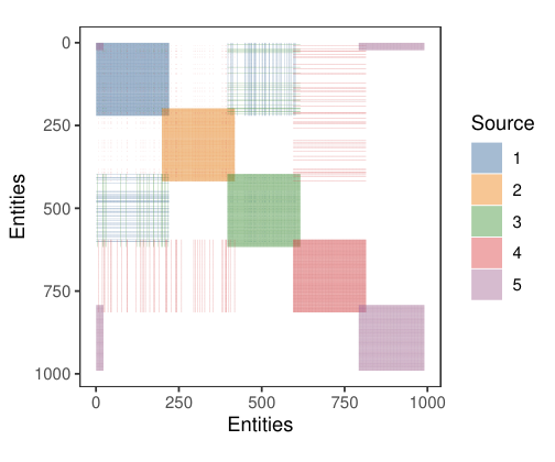
Refer to caption
Figure 5: Observation pattern for the ring-structured block-wise design with random shortcuts, illustrated for m=5m=5 as an example. Each color corresponds to one source, with overlapping regions shown by blended colors where blocks share entities.

We generate the population matrix 𝑷=𝑼​𝚲​𝑼⊤\bm{P}=\bm{U}\bm{\Lambda}\bm{U}^{\top} of size NN and rank d=3d=3, where 𝑼∈𝒪N×d\bm{U}\in\mathcal{O}_{N\times d} is randomly generated, 𝚲=diag⁡(λ,34​λ,12​λ)\bm{\Lambda}=\mathrm{diag}(\lambda,\tfrac{3}{4}\lambda,\tfrac{1}{2}\lambda), and λ=N\lambda=N. For each block ii we observe the noisy submatrix 𝑨(i)=𝑷𝒰i,𝒰i+𝑵(i)\bm{A}^{(i)}=\bm{P}_{\mathcal{U}_{i},\mathcal{U}_{i}}+\bm{N}^{(i)}, where 𝑵(i)\bm{N}^{(i)} is a symmetric Gaussian noise matrix generated as in Section 4.1 with noise level σ=1\sigma=1. We fix the overlap size s=0.1​ns=0.1n, corresponding to an overlap ratio of about 0.10.1, and vary the number of sources m∈{5,10,15,20,25}m\in\{5,10,15,20,25\}, choosing nn so that the total size NN remains approximately 10001000 across all settings. Thus, as mm increases, the fraction of observed entries decreases, making the recovery task progressively more challenging.

The block-wise missing pattern leaves a large fraction of the entries of 𝑷\bm{P} never observed by any source, and we focus on the accuracy of recovering these unobserved entries. Specifically, we report the unobserved relative error, defined as ‖(𝑷^−𝑷)∘𝕀Ωc‖F/‖𝑷∘𝕀Ωc‖F\|(\widehat{\bm{P}}-\bm{P})\circ\mathbb{I}_{\Omega^{c}}\|_{F}/\|\bm{P}\circ\mathbb{I}_{\Omega^{c}}\|_{F}, where Ωc\Omega^{c} denotes the set of entries not observed by any submatrix, together with the running time. Figure 6 reports both quantities, averaged over 100100 Monte Carlo replicates.

As shown in the left panel of Figure 6, GSMMI and CMMI substantially outperform all four matrix-completion baselines. This confirms that, as in Zheng and Tang (2026), methods that exploit the block structure are far more accurate than generic completion methods when the missing pattern is block-wise. The left panel also shows that GSMMI is uniformly more accurate, with the gap widening sharply as mm grows: at m=5m=5 the two methods are nearly identical (0.1160.116 versus 0.1200.120), whereas at m=25m=25 GSMMI attains an unobserved relative error of 0.5240.524 against 0.8480.848 for CMMI, a relative reduction of about 38%38\%. This is consistent with the mechanism identified in Section 4.2: as mm increases and the overlap graph becomes richer in cycles, the advantage of GSMMI over CMMI becomes more pronounced. Finally, the right panel shows that both source-based methods remain computationally efficient, with running times comparable to the fastest baseline (FALS) and orders of magnitude smaller than the slower ones such as GSR and SVT.

Figure 6: Performance of GSMMI, CMMI, and four matrix-completion baselines (FALS, USVT, GSR, SVT) under the ring-structured design with shortcuts described in Section 4.3, as the number of sources mm varies over {5,10,15,20,25}\{5,10,15,20,25\}, with overlap size s=0.1​ns=0.1n, total size N≈1000N\approx 1000, d=3d=3, and σ=1\sigma=1. Left: unobserved relative Frobenius error, ‖(𝑷^−𝑷)∘𝕀Ωc‖F/‖𝑷∘𝕀Ωc‖F\|(\widehat{\bm{P}}-\bm{P})\circ\mathbb{I}_{\Omega^{c}}\|_{F}/\|\bm{P}\circ\mathbb{I}_{\Omega^{c}}\|_{F}; the yy-axis is capped at 1.051.05 for readability, and USVT (with errors up to 2.22.2) exceeds this range. Right: running time in seconds (log scale). Results are averaged over 100100 independent Monte Carlo replicates.

5 Experiments on Realistic Data

In this section, we use two real data examples to demonstrate that GSMMI can further improve upon CMMI in practice. We first consider the MNIST database of handwritten digit images (Section 5.1), and then the MEDLINE co-occurrence database (Section 5.2).

5.1 MNIST handwritten digits

We illustrate the advantage of GSMMI over CMMI and several existing matrix-completion methods on the MNIST database of handwritten digit images (43). The MNIST database consists of grayscale images of handwritten digits, each of size 28×2828\times 28 pixels and viewed as a vector in ℝ784\mathbb{R}^{784}. We consider a population of NN entities, each assigned a fixed label drawn uniformly from the digits {3,5,8}\{3,5,8\}, which are relatively difficult to distinguish. The mm sources are arranged in the same ring-structured block design with random shortcuts as in Section 4.3. For each number of observed blocks mm, we choose the block size nn so that the total number of entities NN remains approximately 30003000 across all settings. For each entity in a given source, we sample an image uniformly at random from the MNIST images sharing its label and normalize it to unit norm. As a result, the same entity is represented by different images of the same digit across sources, which serves as a source of noise. We then form the observed block 𝑨(i)=𝑴(i)​𝑴(i)⊤∈ℝn×n\bm{A}^{(i)}=\bm{M}^{(i)}\bm{M}^{(i)\top}\in\mathbb{R}^{n\times n}, where 𝑴(i)∈ℝn×784\bm{M}^{(i)}\in\mathbb{R}^{n\times 784} stacks the nn unit-normalized images for the entities in source ii.

Given the collection {𝑨(i)}i=1m\{\bm{A}^{(i)}\}_{i=1}^{m}, we compare how accurately different methods can cluster the entities by their underlying digit. We apply CMMI and GSMMI to recover the latent positions of all entities, using embedding dimension d=36d=36, chosen by applying the dimensionality selection procedure of Zhu and Ghodsi (2006) to the MNIST images. For comparison, we also include three of the matrix-completion baselines from Section 4.3, namely GSR, FALS, and USVT; SVT is excluded here because it is prohibitively slow on matrices of this larger size.

We evaluate the clustering accuracy of each method as follows. CMMI and GSMMI directly return dd-dimensional latent positions, which we cluster into three groups using KK-means. The matrix-completion baselines instead return a completed matrix: for these, we first assemble a single partially observed N×NN\times N similarity matrix from the mm source blocks, in which unobserved pairs are left missing and entries observed by multiple sources are averaged; we then apply each completion method to fill in the full matrix, extract its leading dd-dimensional eigen-embedding, and cluster the embedding with KK-means. We measure accuracy against the true digit labels using the Adjusted Rand Index (ARI), which ranges from −1-1 to 11, with higher values indicating closer agreement. We vary the number of sources over m∈{3,4,5,6,7,8,9}m\in\{3,4,5,6,7,8,9\} and report results averaged over 2525 Monte Carlo replicates.

As seen in the left panel of Figure 7, GSMMI and CMMI substantially outperform all three completion baselines, whose ARIs remain below 0.110.11 across every value of mm, confirming that methods exploiting the block structure are far more effective than generic completion methods again. It also shows that GSMMI is uniformly more accurate than CMMI, and the gap widens sharply as mm grows. The clustering accuracy of CMMI peaks at about 0.410.41 for m=4m=4 and then deteriorates steadily, falling to 0.130.13 at m=9m=9, whereas GSMMI remains stable and high, staying in the range 0.400.40–0.490.49 throughout. As shown in the right panel, GSMMI and CMMI have comparable running times, both orders of magnitude smaller than those of the completion baselines. Thus the substantial accuracy gain of GSMMI over CMMI here is obtained at negligible additional computational cost.

Figure 7: Performance of GSMMI, CMMI, and three matrix-completion baselines (FALS, USVT, GSR) on the MNIST experiment under the ring-structured design with shortcuts described in Section 4.3, as the number of sources mm varies over {3,4,5,6,7,8,9}\{3,4,5,6,7,8,9\}, with entities labeled by the digits {3,5,8}\{3,5,8\}, overlap size s=0.1​ns=0.1n, total size N≈3000N\approx 3000, and embedding dimension d=36d=36. Left: Adjusted Rand Index for clustering against the true digit labels. Right: running time in seconds (log scale). Results are averaged over 2525 independent Monte Carlo replicates.

5.2 MEDLINE co-occurrences

Our second example uses the MEDLINE co-occurrence database (National Library of Medicine, 2023), following the same setting as in Section B.1 of the supplementary material of Zheng and Tang (2026). In that work, CMMI was compared against GSR, FALS, SVT, and USVT, and was shown to substantially outperform all of them in both accuracy and computational efficiency. We therefore omit these baselines and focus our comparison on CMMI, since establishing that GSMMI improves upon CMMI is sufficient to demonstrate its advantage over these competing methods as well.

The MEDLINE co-occurrence database summarizes the MeSH descriptors that co-occur in MEDLINE/PubMed citations over a period of years. A standard approach for handling such data is to transform the (normalized) co-occurrence counts into pointwise mutual information (PMI), an association measure widely used in natural language processing. Specifically, the PMI between two concepts xx and yy is defined as PMI⁡(x,y)=log⁡ℙ⁡(x,y)ℙ⁡(x)​ℙ​(y)\mathrm{PMI}(x,y)=\log\tfrac{\mathbb{P}(x,y)}{\mathbb{P}(x)\mathbb{P}(y)}, where ℙ⁡(x)\mathbb{P}(x) and ℙ⁡(y)\mathbb{P}(y) are the marginal occurrence probabilities of xx and yy, and ℙ⁡(x,y)\mathbb{P}(x,y) is their joint co-occurrence probability.

If we partition the citations by year, each year tends to feature a somewhat different set of frequently occurring clinical concepts, and the PMIs computed among the high-frequency concepts within a given year tend to be more accurate than those involving rarely occurring concepts. Motivated by this observation, we extract the PMIs for the top-frequency concepts in each year and integrate them using CMMI or GSMMI, aiming to recover more accurate co-occurrence relationships between the clinical concepts than the PMIs computed directly from data aggregated across all the years.

Concretely, we consider MEDLINE co-occurrence data from the years 1993 to 2022. For each year, we extract a PMI submatrix based on the co-occurrences of the top 10001000 most frequent clinical concepts. Given a number of observed years KK, equivalently the number of observed PMI submatrices, our goal is to integrate these submatrices to recover the full PMI matrix over the union of concepts. In this experiment, we always select the most temporally distant years for the integration task. For example, for K=2K=2 we integrate the PMI submatrices corresponding to the years 19931993 and 20222022, which together involve N=1540N=1540 unique clinical concepts, and we aim to recover the unobserved entries (approximately 25%25\%) in the resulting 1540×15401540\times 1540 PMI matrix. We determine the embedding dimension dd by applying the automatic dimensionality selection procedure of Zhu and Ghodsi (2006) to each observed submatrix and taking the largest resulting value to retain sufficient information. For example, when K=2K=2, the procedure yields dimensions 1212 and 1616 for the two submatrices, so we set d=16d=16. We then apply both CMMI and GSMMI to recover the full PMI matrix.

To evaluate the recovery quality, we use the pre-trained clinical concept embeddings from Beam et al. (2020), which are learned from massive multimodal medical data. Given pre-trained embedding vectors 𝒗1,…,𝒗N\bm{v}_{1},\dots,\bm{v}_{N} for the NN clinical concepts, we construct a similarity matrix 𝑷∈ℝN×N\bm{P}\in\mathbb{R}^{N\times N} whose entry 𝑷i​j\bm{P}_{ij} is the cosine similarity between 𝒗i\bm{v}_{i} and 𝒗j\bm{v}_{j}. We then measure the similarity between the estimated PMIs of the unobserved entries and the corresponding entries in 𝑷\bm{P} using Spearman’s rank correlation ρ\rho, which takes values in [−1,1][-1,1], with larger values indicating a stronger monotone relationship.

We vary KK from 22 to 1515 and report the results in Figure 8. The dashed black line (baseline) in the left panel represents the performance obtained by directly computing PMIs from the co-occurrence data aggregated across the selected years. The results show that integrating per-year PMIs via either CMMI or GSMMI yields substantially more faithful co-occurrence relationships than directly computing PMIs from aggregated data. For instance, when K=2K=2, the baseline achieves a rank correlation of only 0.0480.048, whereas both CMMI and GSMMI reach 0.2730.273. In addition, and more importantly for our purpose, GSMMI consistently matches or exceeds CMMI across all values of KK. When K=2K=2, the two methods coincide exactly, since a single pair of overlapping blocks admits no cycles and the spanning tree already exploits all available overlap information. For larger KK, GSMMI yields a consistent improvement by leveraging the full overlapping structure rather than only a spanning tree, as shown more clearly in the middle panel, which zooms in on the two methods. Moreover, as shown in the right panel, GSMMI attains this improvement at a computational cost very close to that of CMMI.

Figure 8: Performance of GSMMI and CMMI on MEDLINE co-occurrences experiment, integrating per-year PMI submatrices as KK varies from 22 to 1515. On the x-axis, each KK is followed (in parentheses) by the proportion of unobserved entries to be recovered. Left: Spearman’s rank correlation between the recovered PMIs and the clinical concept embeddings of Beam et al. (2020), for the baseline (PMIs computed directly from the co-occurrence data aggregated across the selected years), CMMI, and GSMMI. Middle: the same correlation, zoomed in to compare CMMI and GSMMI. Right: running time in seconds.

6 Extensions to Indefinite and Rectangular Matrices

The GSMMI algorithm presented in Section 2 assumes that the population matrix 𝑷\bm{P} is positive semidefinite, a setting we used to introduce the main idea of the method and to develop its analysis. In many real-world applications, however, the matrix of interest can instead be symmetric but indefinite, or asymmetric and possibly rectangular. Symmetric indefinite matrices arise, for example, in generalized random dot product graph models (Rubin-Delanchy et al., 2022) and in similarity or kernel matrices induced by indefinite kernels, whereas asymmetric or rectangular matrices are central to applications such as genomic data integration (Letunic et al., 2004), single-cell data integration (Stuart et al., 2019), and recommendation systems. Integrating multiple such matrices from different sources naturally leads to multiple matrix integration problems in these non-positive-semidefinite settings.

In this section, we describe how GSMMI can be extended to the cases of symmetric indefinite matrices and asymmetric or rectangular matrices. As in the positive semidefinite setting, the main idea is that GSMMI replaces the spanning-tree alignment of CMMI with a global synchronization over all pairwise overlaps, while providing modifications appropriate to each case. These modifications are also important for the practical feasibility and effectiveness of the algorithm. For example, for symmetric indefinite matrices, the alignment matrices should be indefinite orthogonal matrices, but no direct fast optimizer over the indefinite orthogonal group is available; we therefore approximate the per-iteration solution by relaxing the problem into unconstrained least-squares problems and then projecting the result back onto the indefinite orthogonal group. As another example, for asymmetric or rectangular matrices, the alignment matrices are general invertible matrices, and without care the iterations may accumulate scale drift; we therefore rescale the estimates during the iterations to keep them well-conditioned and improve numerical stability. Other modifications, including appropriate choices of the related weights in each setting, are introduced to make GSMMI effective across these different matrix types.

6.1 GSMMI for symmetric indefinite matrices

Suppose 𝑷∈ℝN×N\bm{P}\in\mathbb{R}^{N\times N} is a symmetric indefinite low-rank matrix. Let d+d_{+} and d−d_{-} denote the number of positive and negative eigenvalues of 𝑷\bm{P}, and set d=d++d−≪Nd=d_{+}+d_{-}\ll N. We denote the non-zero eigenvalues of 𝑷\bm{P} by λ1​(𝑷)≥⋯≥λd+​(𝑷)>0>λN−d−+1​(𝑷)≥⋯≥λN​(𝑷)\lambda_{1}(\bm{P})\geq\dots\geq\lambda_{d_{+}}(\bm{P})>0>\lambda_{N-d_{-}+1}(\bm{P})\geq\dots\geq\lambda_{N}(\bm{P}). Let 𝚲+:=diag⁡(λ1​(𝑷),…,λd+​(𝑷))\bm{\Lambda}_{+}:=\mathrm{diag}(\lambda_{1}(\bm{P}),\dots,\lambda_{d_{+}}(\bm{P})), 𝚲−:=diag⁡(λN−d−+1​(𝑷),…,λN​(𝑷))\bm{\Lambda}_{-}:=\mathrm{diag}(\lambda_{N-d_{-}+1}(\bm{P}),\dots,\lambda_{N}(\bm{P})), and let the orthonormal columns of 𝑼+∈ℝN×d+\bm{U}_{+}\in\mathbb{R}^{N\times d_{+}} and 𝑼−∈ℝN×d−\bm{U}_{-}\in\mathbb{R}^{N\times d_{-}} constitute the corresponding eigenvectors. The eigendecomposition of 𝑷\bm{P} is then 𝑼​𝚲​𝑼⊤\bm{U}\bm{\Lambda}\bm{U}^{\top} with 𝚲:=diag⁡(𝚲+,𝚲−)\bm{\Lambda}:=\mathrm{diag}(\bm{\Lambda}_{+},\bm{\Lambda}_{-}) and 𝑼:=[𝑼+|𝑼−]\bm{U}:=[\bm{U}_{+}|\bm{U}_{-}]. The latent positions are given by 𝑿=𝑼​|𝚲|1/2\bm{X}=\bm{U}|\bm{\Lambda}|^{1/2}, so that 𝑷=𝑿​𝑰d+,d−​𝑿⊤\bm{P}=\bm{X}\bm{I}_{d_{+},d_{-}}\bm{X}^{\top}, where 𝑰d+,d−=diag⁡(𝑰d+,−𝑰d−)\bm{I}_{d_{+},d_{-}}=\mathrm{diag}(\bm{I}_{d_{+}},-\bm{I}_{d_{-}}). For each source ii, we have 𝑷(i)=𝑷𝒰i,𝒰i=𝑿𝒰i​𝑰d+,d−​𝑿𝒰i⊤\bm{P}^{(i)}=\bm{P}_{\mathcal{U}_{i},\mathcal{U}_{i}}=\bm{X}_{\mathcal{U}_{i}}\bm{I}_{d_{+},d_{-}}\bm{X}_{\mathcal{U}_{i}}^{\top}.

From each observed submatrix 𝑨(i)\bm{A}^{(i)}, we obtain an estimated latent position matrix 𝑿^(i)∈ℝni×d\widehat{\bm{X}}^{(i)}\in\mathbb{R}^{n_{i}\times d} such that 𝑨(i)≈𝑿^(i)​𝑰d+,d−​𝑿^(i)⊤\bm{A}^{(i)}\approx\widehat{\bm{X}}^{(i)}\bm{I}_{d_{+},d_{-}}\widehat{\bm{X}}^{(i)\top}. As in the positive semidefinite case (see Remark 1), various methods can be used to obtain such an estimate; for example, one may set 𝑿^(i)=𝑼^(i)​|𝚲^(i)|1/2\widehat{\bm{X}}^{(i)}=\widehat{\bm{U}}^{(i)}|\widehat{\bm{\Lambda}}^{(i)}|^{1/2}, where 𝚲^(i)\widehat{\bm{\Lambda}}^{(i)} collects the d+d_{+} largest positive and d−d_{-} largest (in magnitude) negative eigenvalues of 𝑨(i)\bm{A}^{(i)}, and 𝑼^(i)\widehat{\bm{U}}^{(i)} contains the corresponding eigenvectors.

Each 𝑿^(i)\widehat{\bm{X}}^{(i)} estimates 𝑿𝒰i\bm{X}_{\mathcal{U}_{i}} only up to a transformation, which is now an element of the indefinite orthogonal group 𝒪d+,d−:={𝑶∈ℝd×d:𝑶​𝑰d+,d−​𝑶⊤=𝑰d+,d−}\mathcal{O}_{d_{+},d_{-}}:=\{\bm{O}\in\mathbb{R}^{d\times d}:\bm{O}\bm{I}_{d_{+},d_{-}}\bm{O}^{\top}=\bm{I}_{d_{+},d_{-}}\}. To exploit all pairwise overlaps, we again formulate the alignment as a synchronization problem, seeking transformation matrices {𝑾^(i)}\{\widehat{\bm{W}}^{(i)}\} that jointly align all estimated latent positions across all overlapping entities:

{𝑾^(i)}i=1m=argmin𝑶(1),…,𝑶(m)∈𝒪d+,d−∑i<j:𝒰i∩𝒰j≠∅πi,j∥𝑿^⟨𝒰i∩𝒰j⟩(i)𝑶(i)−𝑿^⟨𝒰i∩𝒰j⟩(j)𝑶(j)∥F2.\{\widehat{\bm{W}}^{(i)}\}_{i=1}^{m}=\argmin_{\bm{O}^{(1)},\ldots,\bm{O}^{(m)}\in\mathcal{O}_{d_{+},d_{-}}}\sum_{i<j:\mathcal{U}_{i}\cap\mathcal{U}_{j}\neq\varnothing}\pi_{i,j}\,\|\widehat{\bm{X}}^{(i)}_{\langle\mathcal{U}_{i}\cap\mathcal{U}_{j}\rangle}\bm{O}^{(i)}-\widehat{\bm{X}}^{(j)}_{\langle\mathcal{U}_{i}\cap\mathcal{U}_{j}\rangle}\bm{O}^{(j)}\|_{F}^{2}.

We again fix 𝑾^(1)=𝑰d\widehat{\bm{W}}^{(1)}=\bm{I}_{d} as the reference and iteratively update each 𝑾^(i)\widehat{\bm{W}}^{(i)} for i=2,…,mi=2,\ldots,m, initializing from the CMMI solution. For a fixed set of transformation matrices {𝑾^(j)}j≠i\{\widehat{\bm{W}}^{(j)}\}_{j\neq i}, using the indefinite orthogonality of 𝑶∈𝒪d+,d−\bm{O}\in\mathcal{O}_{d_{+},d_{-}}, the optimal update for 𝑾^(i)\widehat{\bm{W}}^{(i)} can be written equivalently as

𝑾^(i)\displaystyle\widehat{\bm{W}}^{(i)} =argmin𝑶∈𝒪d+,d−∑j≠i:𝒰i∩𝒰j≠∅πi,j∥𝑿^(i)⟨𝒰i∩𝒰j⟩𝑶−𝑿^(j)⟨𝒰i∩𝒰j⟩𝑾^(j)∥F2\displaystyle=\argmin_{\bm{O}\in\mathcal{O}_{d_{+},d_{-}}}\sum_{j\neq i:\mathcal{U}_{i}\cap\mathcal{U}_{j}\neq\varnothing}\pi_{i,j}\,\|\widehat{\bm{X}}^{(i)}_{\langle\mathcal{U}_{i}\cap\mathcal{U}_{j}\rangle}\bm{O}-\widehat{\bm{X}}^{(j)}_{\langle\mathcal{U}_{i}\cap\mathcal{U}_{j}\rangle}\widehat{\bm{W}}^{(j)}\|_{F}^{2}
=argmin𝑶∈𝒪d+,d−∑j≠i:𝒰i∩𝒰j≠∅πi,j∥𝑿^(i)⟨𝒰i∩𝒰j⟩𝑰d+,d−−𝑿^(j)⟨𝒰i∩𝒰j⟩𝑾^(j)𝑰d+,d−𝑶⊤∥F2.\displaystyle=\argmin_{\bm{O}\in\mathcal{O}_{d_{+},d_{-}}}\sum_{j\neq i:\mathcal{U}_{i}\cap\mathcal{U}_{j}\neq\varnothing}\pi_{i,j}\,\|\widehat{\bm{X}}^{(i)}_{\langle\mathcal{U}_{i}\cap\mathcal{U}_{j}\rangle}\bm{I}_{d_{+},d_{-}}-\widehat{\bm{X}}^{(j)}_{\langle\mathcal{U}_{i}\cap\mathcal{U}_{j}\rangle}\widehat{\bm{W}}^{(j)}\bm{I}_{d_{+},d_{-}}\bm{O}^{\top}\|_{F}^{2}.

But there is no longer an analytical solution due to the indefinite orthogonality constraint, so we approximate the solution by relaxing the problem into two unconstrained least squares problems

𝑾^L(i)\displaystyle\widehat{\bm{W}}_{L}^{(i)} =argmin𝑶∈ℝd×d∑j≠i:𝒰i∩𝒰j≠∅πi,j∥𝑿^(i)⟨𝒰i∩𝒰j⟩𝑶−𝑿^(j)⟨𝒰i∩𝒰j⟩𝑾^(j)∥F2,\displaystyle=\argmin_{\bm{O}\in\mathbb{R}^{d\times d}}\sum_{j\neq i:\mathcal{U}_{i}\cap\mathcal{U}_{j}\neq\varnothing}\pi_{i,j}\,\|\widehat{\bm{X}}^{(i)}_{\langle\mathcal{U}_{i}\cap\mathcal{U}_{j}\rangle}\bm{O}-\widehat{\bm{X}}^{(j)}_{\langle\mathcal{U}_{i}\cap\mathcal{U}_{j}\rangle}\widehat{\bm{W}}^{(j)}\|_{F}^{2}, (6.1)
𝑾^R(i)\displaystyle\widehat{\bm{W}}_{R}^{(i)} =argmin𝑶∈ℝd×d∑j≠i:𝒰i∩𝒰j≠∅πi,j∥𝑿^(i)⟨𝒰i∩𝒰j⟩𝑰d+,d−−𝑿^(j)⟨𝒰i∩𝒰j⟩𝑾^(j)𝑰d+,d−𝑶⊤∥F2.\displaystyle=\argmin_{\bm{O}\in\mathbb{R}^{d\times d}}\sum_{j\neq i:\mathcal{U}_{i}\cap\mathcal{U}_{j}\neq\varnothing}\pi_{i,j}\,\|\widehat{\bm{X}}^{(i)}_{\langle\mathcal{U}_{i}\cap\mathcal{U}_{j}\rangle}\bm{I}_{d_{+},d_{-}}-\widehat{\bm{X}}^{(j)}_{\langle\mathcal{U}_{i}\cap\mathcal{U}_{j}\rangle}\widehat{\bm{W}}^{(j)}\bm{I}_{d_{+},d_{-}}\bm{O}^{\top}\|_{F}^{2}. (6.2)

The solution to (6.1) is

𝑾^L(i)=(∑j≠i:𝒰i∩𝒰j≠∅πi,j(𝑿^⟨𝒰i∩𝒰j⟩(i))⊤𝑿^⟨𝒰i∩𝒰j⟩(i))+(∑j≠i:𝒰i∩𝒰j≠∅πi,j(𝑿^⟨𝒰i∩𝒰j⟩(i))⊤𝑿^⟨𝒰i∩𝒰j⟩(j)𝑾^(j)),\widehat{\bm{W}}_{L}^{(i)}=\Biggl(\sum_{j\neq i:\mathcal{U}_{i}\cap\mathcal{U}_{j}\neq\varnothing}\pi_{i,j}(\widehat{\bm{X}}^{(i)}_{\langle\mathcal{U}_{i}\cap\mathcal{U}_{j}\rangle})^{\top}\widehat{\bm{X}}^{(i)}_{\langle\mathcal{U}_{i}\cap\mathcal{U}_{j}\rangle}\Biggr)^{+}\Biggl(\sum_{j\neq i:\mathcal{U}_{i}\cap\mathcal{U}_{j}\neq\varnothing}\pi_{i,j}(\widehat{\bm{X}}^{(i)}_{\langle\mathcal{U}_{i}\cap\mathcal{U}_{j}\rangle})^{\top}\widehat{\bm{X}}^{(j)}_{\langle\mathcal{U}_{i}\cap\mathcal{U}_{j}\rangle}\widehat{\bm{W}}^{(j)}\Biggr),

where (⋅)+(\cdot)^{+} denotes the Moore-Penrose pseudoinverse. Similarly, the solution to (6.2) is

𝑾^R(i)=\displaystyle\widehat{\bm{W}}_{R}^{(i)}= (∑j≠i:𝒰i∩𝒰j≠∅πi,j𝑰d+,d−(𝑿^(i)⟨𝒰i∩𝒰j⟩)⊤𝑿^(j)⟨𝒰i∩𝒰j⟩𝑾^(j)𝑰d+,d−)\displaystyle\Biggl(\sum_{j\neq i:\mathcal{U}_{i}\cap\mathcal{U}_{j}\neq\varnothing}\pi_{i,j}\,\bm{I}_{d_{+},d_{-}}(\widehat{\bm{X}}^{(i)}_{\langle\mathcal{U}_{i}\cap\mathcal{U}_{j}\rangle})^{\top}\widehat{\bm{X}}^{(j)}_{\langle\mathcal{U}_{i}\cap\mathcal{U}_{j}\rangle}\widehat{\bm{W}}^{(j)}\bm{I}_{d_{+},d_{-}}\Biggr)
(∑j≠i:𝒰i∩𝒰j≠∅πi,j𝑰d+,d−(𝑾^(j))⊤(𝑿^(j)⟨𝒰i∩𝒰j⟩)⊤𝑿^(j)⟨𝒰i∩𝒰j⟩𝑾^(j)𝑰d+,d−)+.\displaystyle\Biggl(\sum_{j\neq i:\mathcal{U}_{i}\cap\mathcal{U}_{j}\neq\varnothing}\pi_{i,j}\,\bm{I}_{d_{+},d_{-}}(\widehat{\bm{W}}^{(j)})^{\top}(\widehat{\bm{X}}^{(j)}_{\langle\mathcal{U}_{i}\cap\mathcal{U}_{j}\rangle})^{\top}\widehat{\bm{X}}^{(j)}_{\langle\mathcal{U}_{i}\cap\mathcal{U}_{j}\rangle}\widehat{\bm{W}}^{(j)}\bm{I}_{d_{+},d_{-}}\Biggr)^{+}.

We combine them by setting 𝑾^(i)=12​(𝑾^L(i)+𝑾^R(i))\widehat{\bm{W}}^{(i)}=\frac{1}{2}(\widehat{\bm{W}}_{L}^{(i)}+\widehat{\bm{W}}_{R}^{(i)}). Since the relaxation drops the indefinite orthogonality constraint, so we project it back onto 𝒪d+,d−\mathcal{O}_{d_{+},d_{-}} before the next update, which improves numerical stability and accuracy. The projection is carried out by taking a few gradient-type steps that iteratively reduce the constraint violation ‖𝑶​𝑰d+,d−​𝑶⊤−𝑰d+,d−‖F\|\bm{O}\,\bm{I}_{d_{+},d_{-}}\,\bm{O}^{\top}-\bm{I}_{d_{+},d_{-}}\|_{F}, starting from 𝑶=𝑾^(i)\bm{O}=\widehat{\bm{W}}^{(i)}. Only a few iterations are needed in practice. We cycle through the updates for i=2,…,mi=2,\ldots,m until convergence. After obtaining {𝑾^(i)}\{\widehat{\bm{W}}^{(i)}\}, we aggregate the aligned latent positions to form 𝑿^\widehat{\bm{X}}, and estimate 𝑷^=𝑿^​𝑰d+,d−​𝑿^⊤\widehat{\bm{P}}=\widehat{\bm{X}}\bm{I}_{d_{+},d_{-}}\widehat{\bm{X}}^{\top}. The complete procedure is summarized in Algorithm 2.

Algorithm 2 GSMMI for symmetric indefinite matrices
0:  Observed submatrices {𝑨(i)}i∈[m]\{\bm{A}^{(i)}\}_{i\in[m]} with index sets {𝒰i}i∈[m]⊆[N]\{\mathcal{U}_{i}\}_{i\in[m]}\subseteq[N], embedding dimensions d+d_{+} and d−d_{-} with d=d++d−d=d_{+}+d_{-}.
 Step 1: Obtain local latent position estimations {X^(i)}i∈[m]\{\widehat{\bm{X}}^{(i)}\}_{i\in[m]}
 Obtain 𝑿^(i)∈ℝni×d\widehat{\bm{X}}^{(i)}\in\mathbb{R}^{n_{i}\times d} such that 𝑨(i)≈𝑿^(i)​𝑰d+,d−​𝑿^(i)⊤\bm{A}^{(i)}\approx\widehat{\bm{X}}^{(i)}\bm{I}_{d_{+},d_{-}}\widehat{\bm{X}}^{(i)\top} for each i∈[m]i\in[m], where ni=|𝒰i|n_{i}=|\mathcal{U}_{i}|.
 Step 2: Obtain alignment matrices {W^(i)}i∈[m]\{\widehat{\bm{W}}^{(i)}\}_{i\in[m]} via synchronization
 Compute the error measure ci:=‖(𝑨(i)−𝑷^(i))​𝑿^(i)​(𝑿^(i)⊤​𝑿^(i))−1​𝑰d+,d−‖F/ni1/2c_{i}:=\|(\bm{A}^{(i)}-\widehat{\bm{P}}^{(i)})\widehat{\bm{X}}^{(i)}(\widehat{\bm{X}}^{(i)\top}\widehat{\bm{X}}^{(i)})^{-1}\bm{I}_{d_{+},d_{-}}\|_{F}/n_{i}^{1/2} for each i∈[m]i\in[m], where 𝑷^(i):=𝑿^(i)​𝑰d+,d−​𝑿^(i)⊤\widehat{\bm{P}}^{(i)}:=\widehat{\bm{X}}^{(i)}\bm{I}_{d_{+},d_{-}}\widehat{\bm{X}}^{(i)\top}.
 Compute the weight πi,j:=(ci2+cj2)−1\pi_{i,j}:=(c_{i}^{2}+c_{j}^{2})^{-1} for each overlapping pair (i,j)(i,j) with 𝒰i∩𝒰j≠∅\mathcal{U}_{i}\cap\mathcal{U}_{j}\neq\varnothing.
 Solve for {𝑾^(i)}i∈[m]\{\widehat{\bm{W}}^{(i)}\}_{i\in[m]} by
{𝑾^(i)}i=1m=argmin𝑶(1),…,𝑶(m)∈𝒪d+,d−∑(i,j):𝒰i∩𝒰j≠∅πi,j∥𝑿^⟨𝒰i∩𝒰j⟩(i)𝑶(i)−𝑿^⟨𝒰i∩𝒰j⟩(j)𝑶(j)∥F2\{\widehat{\bm{W}}^{(i)}\}_{i=1}^{m}=\argmin_{\bm{O}^{(1)},\ldots,\bm{O}^{(m)}\in\mathcal{O}_{d_{+},d_{-}}}\sum_{\begin{subarray}{c}(i,j):\\ \mathcal{U}_{i}\cap\mathcal{U}_{j}\neq\varnothing\end{subarray}}\pi_{i,j}\,\|\widehat{\bm{X}}^{(i)}_{\langle\mathcal{U}_{i}\cap\mathcal{U}_{j}\rangle}\bm{O}^{(i)}-\widehat{\bm{X}}^{(j)}_{\langle\mathcal{U}_{i}\cap\mathcal{U}_{j}\rangle}\bm{O}^{(j)}\|_{F}^{2}
using the alternating optimization based on (6.1) and (6.2) with averaging and projection onto 𝒪d+,d−\mathcal{O}_{d_{+},d_{-}}, 𝑾^(1)=𝑰d\widehat{\bm{W}}^{(1)}=\bm{I}_{d} fixed, and initialization from CMMI.
 Step 3: Aggregate {X^(i)​W^(i)}i∈[m]\{\widehat{\bm{X}}^{(i)}\widehat{\bm{W}}^{(i)}\}_{i\in[m]}
 Compute the weight τi:=ci−2\tau_{i}:=c_{i}^{-2} for each i∈[m]i\in[m].
 Compute the weighted average 𝒙^k=∑i:k∈𝒰iτi(𝑿^(i)𝑾^(i))⟨k⟩∑i:k∈𝒰iτi\widehat{\bm{x}}_{k}=\frac{\sum_{i:k\in\mathcal{U}_{i}}\tau_{i}(\widehat{\bm{X}}^{(i)}\widehat{\bm{W}}^{(i)})_{\langle k\rangle}}{\sum_{i:k\in\mathcal{U}_{i}}\tau_{i}} for each k∈[N]k\in[N].
 Form 𝑿^=[𝒙^1​|⋯|​𝒙^N]⊤\widehat{\bm{X}}=[\widehat{\bm{x}}_{1}|\cdots|\widehat{\bm{x}}_{N}]^{\top} and compute 𝑷^=𝑿^​𝑰d+,d−​𝑿^⊤\widehat{\bm{P}}=\widehat{\bm{X}}\bm{I}_{d_{+},d_{-}}\widehat{\bm{X}}^{\top}.
 Estimated latent position matrix 𝑿^\widehat{\bm{X}} and estimated complete matrix 𝑷^\widehat{\bm{P}}.

We compare GSMMI for symmetric indefinite matrices in Algorithm 2 with CMMI and the four matrix-completion baselines under the same ring-structured block design as in Section 4.3, the difference being that we now take 𝚲=diag⁡(λ,34​λ,−12​λ)\bm{\Lambda}=\mathrm{diag}(\lambda,\tfrac{3}{4}\lambda,-\tfrac{1}{2}\lambda), so that 𝑷\bm{P} is indefinite with d+=2d_{+}=2 positive and d−=1d_{-}=1 negative eigenvalues. Other settings, including the evaluation by the unobserved relative error, are as in Section 4.3. As shown in Figure 9, GSMMI and CMMI again substantially outperform all baselines, and GSMMI is uniformly more accurate than CMMI, with the gap widening sharply as mm grows: at m=21m=21, GSMMI attains an error of 0.3240.324 against 0.7920.792 for CMMI, a relative reduction of about 59%59\%. The running times of GSMMI and CMMI remain comparable and orders of magnitude smaller than the slower baselines.

Figure 9: Performance of GSMMI, CMMI, and four matrix-completion baselines (FALS, USVT, GSR, SVT) for symmetric indefinite matrices under the ring-structured design with shortcuts described in Section 4.3, with 𝚲=diag⁡(λ,34​λ,−12​λ)\bm{\Lambda}=\mathrm{diag}(\lambda,\tfrac{3}{4}\lambda,-\tfrac{1}{2}\lambda) (d+=2d_{+}=2, d−=1d_{-}=1), as mm varies over {5,9,13,17,21}\{5,9,13,17,21\}. Other settings are as in Figure 6. Left: unobserved relative Frobenius error; the yy-axis is capped at 1.051.05 for readability, and USVT (with errors up to 1.81.8) exceeds this range. Right: running time in seconds (log scale). Results are averaged over 100100 independent Monte Carlo replicates.

6.2 GSMMI for asymmetric or rectangular matrices

Suppose 𝑷∈ℝN×M\bm{P}\in\mathbb{R}^{N\times M} is a low-rank matrix of rank dd, with singular value decomposition 𝑷=𝑼​𝚺​𝑽⊤\bm{P}=\bm{U}\bm{\Sigma}\bm{V}^{\top}, where 𝚺∈ℝd×d\bm{\Sigma}\in\mathbb{R}^{d\times d} contains the singular values in descending order, and the orthonormal columns of 𝑼∈ℝN×d\bm{U}\in\mathbb{R}^{N\times d} and 𝑽∈ℝM×d\bm{V}\in\mathbb{R}^{M\times d} are the left and right singular vectors. The left and right latent positions are 𝑿=𝑼​𝚺1/2∈ℝN×d\bm{X}=\bm{U}\bm{\Sigma}^{1/2}\in\mathbb{R}^{N\times d} and 𝒀=𝑽​𝚺1/2∈ℝM×d\bm{Y}=\bm{V}\bm{\Sigma}^{1/2}\in\mathbb{R}^{M\times d}, so that 𝑷=𝑿​𝒀⊤\bm{P}=\bm{X}\bm{Y}^{\top}. For source ii, let 𝒰i⊆[N]\mathcal{U}_{i}\subseteq[N] and 𝒱i⊆[M]\mathcal{V}_{i}\subseteq[M] denote the row and column index sets, so that 𝑷(i)=𝑷𝒰i,𝒱i=𝑿𝒰i​𝒀𝒱i⊤\bm{P}^{(i)}=\bm{P}_{\mathcal{U}_{i},\mathcal{V}_{i}}=\bm{X}_{\mathcal{U}_{i}}\bm{Y}_{\mathcal{V}_{i}}^{\top}.

From each observed 𝑨(i)\bm{A}^{(i)}, we obtain estimated left and right latent positions (𝑿^(i),𝒀^(i))(\widehat{\bm{X}}^{(i)},\widehat{\bm{Y}}^{(i)}) such that 𝑨(i)≈𝑿^(i)​𝒀^(i)⊤\bm{A}^{(i)}\approx\widehat{\bm{X}}^{(i)}\widehat{\bm{Y}}^{(i)\top}. For example, one may set 𝑿^(i)=𝑼^(i)​(𝚺^(i))1/2\widehat{\bm{X}}^{(i)}=\widehat{\bm{U}}^{(i)}(\widehat{\bm{\Sigma}}^{(i)})^{1/2} and 𝒀^(i)=𝑽^(i)​(𝚺^(i))1/2\widehat{\bm{Y}}^{(i)}=\widehat{\bm{V}}^{(i)}(\widehat{\bm{\Sigma}}^{(i)})^{1/2} from the leading singular vectors of 𝑨(i)\bm{A}^{(i)}. Each estimate (𝑿^(i),𝒀^(i))(\widehat{\bm{X}}^{(i)},\widehat{\bm{Y}}^{(i)}) recovers (𝑿𝒰i,𝒀𝒱i)(\bm{X}_{\mathcal{U}_{i}},\bm{Y}_{\mathcal{V}_{i}}) only up to an invertible transformation 𝑾(i)∈ℝd×d\bm{W}^{(i)}\in\mathbb{R}^{d\times d}, which acts on the left latent positions as 𝑿𝒰i=𝑿^(i)​𝑾(i)\bm{X}_{\mathcal{U}_{i}}=\widehat{\bm{X}}^{(i)}\bm{W}^{(i)} and on the right latent positions as 𝒀𝒱i=𝒀^(i)​(𝑾(i)⊤)−1\bm{Y}_{\mathcal{V}_{i}}=\widehat{\bm{Y}}^{(i)}(\bm{W}^{(i)\top})^{-1}.

To globally synchronize all sources, we align the left latent positions across overlapping rows and the right latent positions across overlapping columns simultaneously. A single transformation 𝑾(i)\bm{W}^{(i)} governs both, acting on the left latent positions as 𝑾(i)\bm{W}^{(i)} and on the right latent positions as (𝑾(i)⊤)−1(\bm{W}^{(i)\top})^{-1}. We thus seek transformation matrices {𝑾^(i)}\{\widehat{\bm{W}}^{(i)}\} that jointly minimize

{𝑾^(i)}i=1m=argmin𝑶(1),…,𝑶(m)∈ℝd×d\displaystyle\{\widehat{\bm{W}}^{(i)}\}_{i=1}^{m}=\argmin_{\bm{O}^{(1)},\ldots,\bm{O}^{(m)}\in\mathbb{R}^{d\times d}} ∑i<j:𝒰i∩𝒰j≠∅π𝑿i,j∥𝑿^(i)⟨𝒰i∩𝒰j⟩𝑶(i)−𝑿^(j)⟨𝒰i∩𝒰j⟩𝑶(j)∥F2\displaystyle\sum_{i<j:\mathcal{U}_{i}\cap\mathcal{U}_{j}\neq\varnothing}\pi^{\bm{X}}_{i,j}\,\|\widehat{\bm{X}}^{(i)}_{\langle\mathcal{U}_{i}\cap\mathcal{U}_{j}\rangle}\bm{O}^{(i)}-\widehat{\bm{X}}^{(j)}_{\langle\mathcal{U}_{i}\cap\mathcal{U}_{j}\rangle}\bm{O}^{(j)}\|_{F}^{2} (6.3)
+∑i<j:𝒱i∩𝒱j≠∅π𝒀i,j∥𝒀^(i)⟨𝒱i∩𝒱j⟩(𝑶(i)⊤)−1−𝒀^(j)⟨𝒱i∩𝒱j⟩(𝑶(j)⊤)−1∥F2.\displaystyle+\sum_{i<j:\mathcal{V}_{i}\cap\mathcal{V}_{j}\neq\varnothing}\pi^{\bm{Y}}_{i,j}\,\|\widehat{\bm{Y}}^{(i)}_{\langle\mathcal{V}_{i}\cap\mathcal{V}_{j}\rangle}(\bm{O}^{(i)\top})^{-1}-\widehat{\bm{Y}}^{(j)}_{\langle\mathcal{V}_{i}\cap\mathcal{V}_{j}\rangle}(\bm{O}^{(j)\top})^{-1}\|_{F}^{2}.

Here πi,j𝑿\pi^{\bm{X}}_{i,j} and πi,j𝒀\pi^{\bm{Y}}_{i,j} are the analogues of the weight πi,j\pi_{i,j} used in the previous settings, now computed separately for the row and column overlaps from the corresponding error measures ci𝑿c^{\bm{X}}_{i} and ci𝒀c^{\bm{Y}}_{i} (defined in Algorithm 3), since the left and right latent positions are estimated with different accuracies. The two terms depend on the transformation differently, since the second involves it through (𝑶(i)⊤)−1(\bm{O}^{(i)\top})^{-1}. We therefore solve (6.3) by an alternating scheme initialized from the CMMI solution, with 𝑾^(1)=𝑰d\widehat{\bm{W}}^{(1)}=\bm{I}_{d} fixed as the reference. At each step, to update 𝑾^(i)\widehat{\bm{W}}^{(i)} for i=2,…,mi=2,\ldots,m with the remaining transformations held fixed, we compute two separate least squares estimates. Aligning the left latent positions gives

𝑾^𝑿(i)=argmin𝑶∈ℝd×d∑j≠i:𝒰i∩𝒰j≠∅π𝑿i,j∥𝑿^(i)⟨𝒰i∩𝒰j⟩𝑶−𝑿^(j)⟨𝒰i∩𝒰j⟩𝑾^(j)∥F2,\widehat{\bm{W}}_{\bm{X}}^{(i)}=\argmin_{\bm{O}\in\mathbb{R}^{d\times d}}\sum_{j\neq i:\mathcal{U}_{i}\cap\mathcal{U}_{j}\neq\varnothing}\pi^{\bm{X}}_{i,j}\,\|\widehat{\bm{X}}^{(i)}_{\langle\mathcal{U}_{i}\cap\mathcal{U}_{j}\rangle}\bm{O}-\widehat{\bm{X}}^{(j)}_{\langle\mathcal{U}_{i}\cap\mathcal{U}_{j}\rangle}\widehat{\bm{W}}^{(j)}\|_{F}^{2}, (6.4)

which estimates 𝑾^(i)\widehat{\bm{W}}^{(i)} from the row overlaps, and aligning the right latent positions gives

𝑾^𝒀(i)=argmin𝑶∈ℝd×d∑j≠i:𝒱i∩𝒱j≠∅πi,j𝒀∥𝒀^⟨𝒱i∩𝒱j⟩(i)𝑶−𝒀^⟨𝒱i∩𝒱j⟩(j)(𝑾^(j)⊤)−1∥F2,\widehat{\bm{W}}_{\bm{Y}}^{(i)}=\argmin_{\bm{O}\in\mathbb{R}^{d\times d}}\sum_{j\neq i:\mathcal{V}_{i}\cap\mathcal{V}_{j}\neq\varnothing}\pi^{\bm{Y}}_{i,j}\,\|\widehat{\bm{Y}}^{(i)}_{\langle\mathcal{V}_{i}\cap\mathcal{V}_{j}\rangle}\bm{O}-\widehat{\bm{Y}}^{(j)}_{\langle\mathcal{V}_{i}\cap\mathcal{V}_{j}\rangle}(\widehat{\bm{W}}^{(j)\top})^{-1}\|_{F}^{2}, (6.5)

which estimates (𝑾^(i)⊤)−1(\widehat{\bm{W}}^{(i)\top})^{-1} from the column overlaps. Both (6.4) and (6.5) are standard least squares problems with closed-form solutions via the Moore-Penrose pseudoinverse.

Since 𝑾^𝑿(i)\widehat{\bm{W}}_{\bm{X}}^{(i)} and (𝑾^𝒀(i)⊤)−1(\widehat{\bm{W}}_{\bm{Y}}^{(i)\top})^{-1} are both estimates of 𝑾^(i)\widehat{\bm{W}}^{(i)}, we combine them into a single update. Unlike a single-block error, the reliability of each estimate is governed by the amount of overlap information constraining it: 𝑾^𝑿(i)\widehat{\bm{W}}_{\bm{X}}^{(i)} is more reliable when source ii shares more and larger row overlaps with the others, and analogously for (𝑾^𝒀(i)⊤)−1(\widehat{\bm{W}}_{\bm{Y}}^{(i)\top})^{-1} and the column overlaps. We therefore weight the two estimates by the total overlap information they use,

κ𝑿(i):=∑j≠i:𝒰i∩𝒰j≠∅π𝑿i,j∥𝑿^(i)⟨𝒰i∩𝒰j⟩∥F2,κ𝒀(i):=∑j≠i:𝒱i∩𝒱j≠∅π𝒀i,j∥𝒀^(i)⟨𝒱i∩𝒱j⟩∥F2,\kappa_{\bm{X}}^{(i)}:=\sum_{j\neq i:\mathcal{U}_{i}\cap\mathcal{U}_{j}\neq\varnothing}\pi^{\bm{X}}_{i,j}\,\|\widehat{\bm{X}}^{(i)}_{\langle\mathcal{U}_{i}\cap\mathcal{U}_{j}\rangle}\|_{F}^{2},\qquad\kappa_{\bm{Y}}^{(i)}:=\sum_{j\neq i:\mathcal{V}_{i}\cap\mathcal{V}_{j}\neq\varnothing}\pi^{\bm{Y}}_{i,j}\,\|\widehat{\bm{Y}}^{(i)}_{\langle\mathcal{V}_{i}\cap\mathcal{V}_{j}\rangle}\|_{F}^{2}, (6.6)

which equal the traces of the Gram matrices in (6.4) and (6.5) and quantify the total amount of overlap information available in each direction, and update

𝑾^(i)=κ𝑿(i)​𝑾^𝑿(i)+κ𝒀(i)​(𝑾^𝒀(i)⊤)−1κ𝑿(i)+κ𝒀(i).\widehat{\bm{W}}^{(i)}=\frac{\kappa_{\bm{X}}^{(i)}\,\widehat{\bm{W}}_{\bm{X}}^{(i)}+\kappa_{\bm{Y}}^{(i)}\,(\widehat{\bm{W}}_{\bm{Y}}^{(i)\top})^{-1}}{\kappa_{\bm{X}}^{(i)}+\kappa_{\bm{Y}}^{(i)}}. (6.7)

Since the two least squares estimates are unconstrained, the combined 𝑾^(i)\widehat{\bm{W}}^{(i)} may become poorly scaled and accumulate scale drift over the iterations. We therefore rescale its singular values toward unity after each update to keep it well-conditioned, which improves numerical stability. We repeat these updates for i=2,…,mi=2,\ldots,m until convergence. After obtaining {𝑾^(i)}\{\widehat{\bm{W}}^{(i)}\}, we aggregate the aligned left and right latent positions separately, as in (2.5), to form 𝑿^\widehat{\bm{X}} and 𝒀^\widehat{\bm{Y}}, and estimate 𝑷^=𝑿^​𝒀^⊤\widehat{\bm{P}}=\widehat{\bm{X}}\widehat{\bm{Y}}^{\top}. The complete procedure is summarized in Algorithm 3.

We note, as also mentioned for CMMI in Zheng and Tang (2026), that two sources of an asymmetric matrix can be synchronized as long as they share sufficiently many row indices or sufficiently many column indices; overlap in both is not required. This is naturally accommodated by the weighted update (6.7). If source ii has no column overlap with any other source, then κ𝒀(i)=0\kappa_{\bm{Y}}^{(i)}=0 and the update reduces to 𝑾^(i)=𝑾^𝑿(i)\widehat{\bm{W}}^{(i)}=\widehat{\bm{W}}_{\bm{X}}^{(i)}, relying solely on the row overlaps; symmetrically, if it has no row overlap, then κ𝑿(i)=0\kappa_{\bm{X}}^{(i)}=0 and the update reduces to 𝑾^(i)=(𝑾^𝒀(i)⊤)−1\widehat{\bm{W}}^{(i)}=(\widehat{\bm{W}}_{\bm{Y}}^{(i)\top})^{-1}.

Algorithm 3 GSMMI for asymmetric matrices
0:  Observed submatrices {𝑨(i)}i∈[m]\{\bm{A}^{(i)}\}_{i\in[m]} with row and column index sets {(𝒰i,𝒱i)}i∈[m]⊆[N]×[M]\{(\mathcal{U}_{i},\mathcal{V}_{i})\}_{i\in[m]}\subseteq[N]\times[M], embedding dimension dd.
 Step 1: Obtain local latent position estimations {(X^(i),Y^(i))}i∈[m]\{(\widehat{\bm{X}}^{(i)},\widehat{\bm{Y}}^{(i)})\}_{i\in[m]}
 Obtain 𝑿^(i)∈ℝ|𝒰i|×d\widehat{\bm{X}}^{(i)}\in\mathbb{R}^{|\mathcal{U}_{i}|\times d} and 𝒀^(i)∈ℝ|𝒱i|×d\widehat{\bm{Y}}^{(i)}\in\mathbb{R}^{|\mathcal{V}_{i}|\times d} such that 𝑨(i)≈𝑿^(i)​𝒀^(i)⊤\bm{A}^{(i)}\approx\widehat{\bm{X}}^{(i)}\widehat{\bm{Y}}^{(i)\top} for each i∈[m]i\in[m].
 Step 2: Obtain alignment matrices {W^(i)}i∈[m]\{\widehat{\bm{W}}^{(i)}\}_{i\in[m]} via synchronization
 Compute the error measures ci𝑿:=‖(𝑨(i)−𝑷^(i))​𝒀^(i)​(𝒀^(i)⊤​𝒀^(i))−1‖F/|𝒰i|1/2c^{\bm{X}}_{i}:=\|(\bm{A}^{(i)}-\widehat{\bm{P}}^{(i)})\widehat{\bm{Y}}^{(i)}(\widehat{\bm{Y}}^{(i)\top}\widehat{\bm{Y}}^{(i)})^{-1}\|_{F}/|\mathcal{U}_{i}|^{1/2} and ci𝒀:=‖(𝑨(i)−𝑷^(i))⊤​𝑿^(i)​(𝑿^(i)⊤​𝑿^(i))−1‖F/|𝒱i|1/2c^{\bm{Y}}_{i}:=\|(\bm{A}^{(i)}-\widehat{\bm{P}}^{(i)})^{\top}\widehat{\bm{X}}^{(i)}(\widehat{\bm{X}}^{(i)\top}\widehat{\bm{X}}^{(i)})^{-1}\|_{F}/|\mathcal{V}_{i}|^{1/2} for each i∈[m]i\in[m], where 𝑷^(i):=𝑿^(i)​𝒀^(i)⊤\widehat{\bm{P}}^{(i)}:=\widehat{\bm{X}}^{(i)}\widehat{\bm{Y}}^{(i)\top}.
 Compute the weight πi,j𝑿:=((ci𝑿)2+(cj𝑿)2)−1\pi^{\bm{X}}_{i,j}:=((c^{\bm{X}}_{i})^{2}+(c^{\bm{X}}_{j})^{2})^{-1} for each pair with 𝒰i∩𝒰j≠∅\mathcal{U}_{i}\cap\mathcal{U}_{j}\neq\varnothing and the weight πi,j𝒀:=((ci𝒀)2+(cj𝒀)2)−1\pi^{\bm{Y}}_{i,j}:=((c^{\bm{Y}}_{i})^{2}+(c^{\bm{Y}}_{j})^{2})^{-1} for each pair with 𝒱i∩𝒱j≠∅\mathcal{V}_{i}\cap\mathcal{V}_{j}\neq\varnothing.
 Compute the weights κ𝑿i:=∑j≠i:𝒰i∩𝒰j≠∅π𝑿i,j∥𝑿^(i)⟨𝒰i∩𝒰j⟩∥F2\kappa^{\bm{X}}_{i}:=\sum_{j\neq i:\mathcal{U}_{i}\cap\mathcal{U}_{j}\neq\varnothing}\pi^{\bm{X}}_{i,j}\,\|\widehat{\bm{X}}^{(i)}_{\langle\mathcal{U}_{i}\cap\mathcal{U}_{j}\rangle}\|_{F}^{2} and κ𝒀i:=∑j≠i:𝒱i∩𝒱j≠∅π𝒀i,j∥𝒀^(i)⟨𝒱i∩𝒱j⟩∥F2\kappa^{\bm{Y}}_{i}:=\sum_{j\neq i:\mathcal{V}_{i}\cap\mathcal{V}_{j}\neq\varnothing}\pi^{\bm{Y}}_{i,j}\,\|\widehat{\bm{Y}}^{(i)}_{\langle\mathcal{V}_{i}\cap\mathcal{V}_{j}\rangle}\|_{F}^{2} for each i∈[m]i\in[m].
 Solve for {𝑾^(i)}i∈[m]\{\widehat{\bm{W}}^{(i)}\}_{i\in[m]} by
{𝑾^(i)}i=1m=argmin𝑶(1),…,𝑶(m)∈ℝd×d∑i<j:𝒰i∩𝒰j≠∅\displaystyle\{\widehat{\bm{W}}^{(i)}\}_{i=1}^{m}=\argmin_{\bm{O}^{(1)},\ldots,\bm{O}^{(m)}\in\mathbb{R}^{d\times d}}\sum_{\begin{subarray}{c}i<j:\\ \mathcal{U}_{i}\cap\mathcal{U}_{j}\neq\varnothing\end{subarray}} πi,j𝑿​‖𝑿^⟨𝒰i∩𝒰j⟩(i)​𝑶(i)−𝑿^⟨𝒰i∩𝒰j⟩(j)​𝑶(j)‖F2\displaystyle\pi^{\bm{X}}_{i,j}\,\|\widehat{\bm{X}}^{(i)}_{\langle\mathcal{U}_{i}\cap\mathcal{U}_{j}\rangle}\bm{O}^{(i)}-\widehat{\bm{X}}^{(j)}_{\langle\mathcal{U}_{i}\cap\mathcal{U}_{j}\rangle}\bm{O}^{(j)}\|_{F}^{2}
+∑i<j:𝒱i∩𝒱j≠∅π𝒀i,j∥𝒀^(i)⟨𝒱i∩𝒱j⟩(𝑶(i)⊤)−1−𝒀^(j)⟨𝒱i∩𝒱j⟩(𝑶(j)⊤)−1∥F2,\displaystyle+\sum_{\begin{subarray}{c}i<j:\\ \mathcal{V}_{i}\cap\mathcal{V}_{j}\neq\varnothing\end{subarray}}\pi^{\bm{Y}}_{i,j}\,\|\widehat{\bm{Y}}^{(i)}_{\langle\mathcal{V}_{i}\cap\mathcal{V}_{j}\rangle}(\bm{O}^{(i)\top})^{-1}-\widehat{\bm{Y}}^{(j)}_{\langle\mathcal{V}_{i}\cap\mathcal{V}_{j}\rangle}(\bm{O}^{(j)\top})^{-1}\|_{F}^{2},
using the alternating optimization based on (6.4) and (6.5) with the weighted combination (6.7) using κi𝑿,κi𝒀\kappa^{\bm{X}}_{i},\kappa^{\bm{Y}}_{i} and rescaling of the singular values toward unity, with 𝑾^(1)=𝑰d\widehat{\bm{W}}^{(1)}=\bm{I}_{d} fixed and initialization from CMMI.
 Step 3: Aggregate the aligned latent positions
 Compute the weights τi𝑿:=(ci𝑿)−2\tau^{\bm{X}}_{i}:=(c^{\bm{X}}_{i})^{-2} and τi𝒀:=(ci𝒀)−2\tau^{\bm{Y}}_{i}:=(c^{\bm{Y}}_{i})^{-2} for each i∈[m]i\in[m].
 For each row entity k∈[N]k\in[N], compute 𝒙^k=∑i:k∈𝒰iτ𝑿i(𝑿^(i)𝑾^(i))⟨k⟩∑i:k∈𝒰iτ𝑿i\widehat{\bm{x}}_{k}=\frac{\sum_{i:k\in\mathcal{U}_{i}}\tau^{\bm{X}}_{i}(\widehat{\bm{X}}^{(i)}\widehat{\bm{W}}^{(i)})_{\langle k\rangle}}{\sum_{i:k\in\mathcal{U}_{i}}\tau^{\bm{X}}_{i}}, and for each column entity l∈[M]l\in[M], compute 𝒚^l=∑i:l∈𝒱iτ𝒀i(𝒀^(i)(𝑾^(i)⊤)−1)⟨l⟩∑i:l∈𝒱iτ𝒀i\widehat{\bm{y}}_{l}=\frac{\sum_{i:l\in\mathcal{V}_{i}}\tau^{\bm{Y}}_{i}(\widehat{\bm{Y}}^{(i)}(\widehat{\bm{W}}^{(i)\top})^{-1})_{\langle l\rangle}}{\sum_{i:l\in\mathcal{V}_{i}}\tau^{\bm{Y}}_{i}}.
 Form 𝑿^=[𝒙^1​|⋯|​𝒙^N]⊤\widehat{\bm{X}}=[\widehat{\bm{x}}_{1}|\cdots|\widehat{\bm{x}}_{N}]^{\top} and 𝒀^=[𝒚^1​|⋯|​𝒚^M]⊤\widehat{\bm{Y}}=[\widehat{\bm{y}}_{1}|\cdots|\widehat{\bm{y}}_{M}]^{\top}, and compute 𝑷^=𝑿^​𝒀^⊤\widehat{\bm{P}}=\widehat{\bm{X}}\widehat{\bm{Y}}^{\top}.
 Estimated latent position matrices 𝑿^\widehat{\bm{X}} and 𝒀^\widehat{\bm{Y}}, and estimated complete matrix 𝑷^\widehat{\bm{P}}.

We compare GSMMI for asymmetric matrices in Algorithm 3 with CMMI and the four matrix-completion baselines under a ring-structured block design analogous to that in Section 4.3, the only difference being that 𝑷=𝑼​𝚺​𝑽⊤∈ℝN×M\bm{P}=\bm{U}\bm{\Sigma}\bm{V}^{\top}\in\mathbb{R}^{N\times M} is now rectangular, with 𝚺=diag⁡(λ,34​λ,12​λ)\bm{\Sigma}=\mathrm{diag}(\lambda,\tfrac{3}{4}\lambda,\tfrac{1}{2}\lambda), and the ring-and-shortcut structure is applied independently to the row and column index sets, so that each source observes a submatrix of overlapping rows and columns; the left panel of Figure 10 illustrates the resulting observation pattern, taking m=5m=5 as an example. We fix N≈1000N\approx 1000 and M≈1400M\approx 1400, and all other settings, including the evaluation by the unobserved relative error, are as in Section 4.3. As shown in Figure 10, GSMMI and CMMI again substantially outperform all baselines, and GSMMI is uniformly more accurate than CMMI, with the gap widening as mm grows: at m=25m=25, GSMMI attains an error of 0.3260.326 against 0.7320.732 for CMMI, a relative reduction of about 55%55\%. The running times of GSMMI and CMMI remain comparable and orders of magnitude smaller than the slower baselines.

Refer to caption
Figure 10: Performance of GSMMI, CMMI, and four matrix-completion baselines (FALS, USVT, GSR, SVT) for asymmetric matrices under a ring-structured design with shortcuts analogous to Section 4.3, applied independently to rows and columns, with 𝚺=diag⁡(λ,34​λ,12​λ)\bm{\Sigma}=\mathrm{diag}(\lambda,\tfrac{3}{4}\lambda,\tfrac{1}{2}\lambda), as mm varies over {5,10,15,20,25}\{5,10,15,20,25\}, and N≈1000N\approx 1000, M≈1400M\approx 1400. Left: the observation pattern, shown for m=5m=5 as an example, where each color corresponds to one source and overlapping regions are shown by blended colors where blocks share entities. Middle: unobserved relative Frobenius error; the yy-axis is capped at 1.051.05 for readability, and USVT (with errors up to 1.161.16) exceeds this range. Right: running time in seconds (log scale). Results are averaged over 100100 independent Monte Carlo replicates.

As noted above, two sources can be synchronized as long as they share sufficiently many row indices or column indices, so overlap in only one direction already suffices. To illustrate this empirically, we consider a more challenging variant in which the sources share no columns at all: the rows still follow the ring-and-shortcut structure, but the column index sets are disjoint, so that each column entity is observed by exactly one source. Alignment therefore relies entirely on the shared rows, and the column latent positions are recovered indirectly through the row-based synchronization. All other settings are as in the previous asymmetric experiment; the left panel of Figure 11 illustrates the resulting observation pattern for m=5m=5, where the dashed vertical lines mark the boundaries between the disjoint column blocks. As shown in Figure 11, GSMMI and CMMI still substantially outperform all baselines even under this column-disjoint design, and GSMMI remains uniformly more accurate than CMMI, with the gap again widening as mm grows: at m=24m=24, GSMMI attains an error of 0.3790.379 against 0.7040.704 for CMMI, a relative reduction of about 46%46\%. This confirms that GSMMI continues to benefit from global synchronization even when alignment relies entirely on row overlaps. The running times of GSMMI and CMMI remain comparable and orders of magnitude smaller than the slower baselines.

Refer to caption
Figure 11: Performance of GSMMI, CMMI, and four matrix-completion baselines (FALS, USVT, GSR, SVT) for asymmetric matrices under the column-disjoint ring-structured design, where the rows follow the ring-structured design with shortcuts but the column blocks are disjoint, with 𝚺=diag⁡(λ,34​λ,12​λ)\bm{\Sigma}=\mathrm{diag}(\lambda,\tfrac{3}{4}\lambda,\tfrac{1}{2}\lambda), as mm varies over {5,11,16,20,24}\{5,11,16,20,24\}, and N≈1000N\approx 1000, M≈1400M\approx 1400. Left: the observation pattern, shown for m=5m=5 as an example, where each color corresponds to one source and dashed vertical lines mark the boundaries between disjoint column blocks. Middle: unobserved relative Frobenius error; the yy-axis is capped at 1.051.05 for readability, and USVT (with errors up to 1.161.16) exceeds this range. Right: running time in seconds (log scale). Results are averaged over 100100 independent Monte Carlo replicates.

References

  • Abbe et al. (2020) E. Abbe, J. Fan, K. Wang, and Y. Zhong Entrywise eigenvector analysis of random matrices with low expected rank. Annals of Statistics 48, pp. 1452–1474. Cited by: Remark 8.
  • Ahuja et al. (2020) Y. Ahuja, D. Zhou, Z. He, J. Sun, V. M. Castro, V. Gainer, S. N. Murphy, C. Hong, and T. Cai SureLDA: a multidisease automated phenotyping method for the electronic health record. Journal of the American Medical Informatics Association 27, pp. 1235–1243. Cited by: §1.
  • Argelaguet et al. (2021) R. Argelaguet, A. S. Cuomo, O. Stegle, and J. C. Marioni Computational principles and challenges in single-cell data integration. Nature biotechnology 39, pp. 1202–1215. Cited by: §1.
  • Bandeira et al. (2016) A. S. Bandeira, C. Kennedy, and A. Singer Approximating the little grothendieck problem over the orthogonal and unitary groups. Mathematical programming 160 (1), pp. 433–475. Cited by: Appendix A, Remark 3.
  • Beam et al. (2020) A. L. Beam, B. Kompa, A. Schmaltz, I. Fried, G. Weber, N. Palmer, X. Shi, T. Cai, and I. S. Kohane Clinical concept embeddings learned from massive sources of multimodal medical data. In Pacific Symposium on Biocomputing. Pacific Symposium on Biocomputing, Vol. 25, pp. 295. Cited by: Figure 8, Figure 8, §5.2.
  • Benaych-Georges and Nadakuditi (2011) F. Benaych-Georges and R. R. Nadakuditi The eigenvalues and eigenvectors of finite, low rank perturbations of large random matrices. Advances in Mathematics 227 (1), pp. 494–521. Cited by: §B.6.
  • Bishop and Yu (2014) W. E. Bishop and B. M. Yu Deterministic symmetric positive semidefinite matrix completion. Advances in Neural Information Processing Systems 27, pp. 2762–2770. Cited by: §1, §1.
  • Cai et al. (2010) J. Cai, E. J. Candès, and Z. Shen A singular value thresholding algorithm for matrix completion. SIAM Journal on Optimization 20, pp. 1956–1982. Cited by: §4.3.
  • Cai et al. (2016) T. Cai, T. T. Cai, and A. Zhang Structured matrix completion with applications to genomic data integration. Journal of the American Statistical Association 111, pp. 621–633. Cited by: §1.
  • Cai and Zhou (2016) T. Cai and W. Zhou Matrix completion via max-norm constrained optimization. Electronic Journal of Statistics 10, pp. 1493–1525. Cited by: §1.
  • Candes and Plan (2011) E. J. Candes and Y. Plan Tight oracle inequalities for low-rank matrix recovery from a minimal number of noisy random measurements. IEEE Transactions on Information Theory 57, pp. 2342–2359. Cited by: §1.
  • Candes and Recht (2012) E. Candes and B. Recht Exact matrix completion via convex optimization. Communications of the ACM 55, pp. 111–119. Cited by: §1.
  • Chatterjee (2015) S. Chatterjee Matrix estimation by universal singular value thresholding. The annals of statistics, pp. 177–214. Cited by: §4.3, Remark 1.
  • Chen et al. (2020) J. Chen, D. Liu, and X. Li Nonconvex rectangular matrix completion via gradient descent without ℓ2,∞\ell_{2,\infty} regularization. IEEE Transactions on Information Theory 66, pp. 5806–5841. Cited by: §1.
  • Chen and Kunisky (2025) S. Chen and D. Kunisky Universal entrywise eigenvector fluctuations in delocalized spiked matrix models and asymptotics of rounded spectral algorithms. arXiv preprint arXiv:2512.11785. External Links: 2512.11785, Document Cited by: §3.
  • Chen et al. (2021) Y. Chen, Y. Chi, J. Fan, and C. Ma Spectral methods for data science: a statistical perspective. Foundations and Trends® in Machine Learning 14, pp. 566–806. Cited by: Remark 8.
  • Chen et al. (2019) Y. Chen, J. Fan, C. Ma, and Y. Yan Inference and uncertainty quantification for noisy matrix completion. PNAS 116, pp. 22931–22937. Cited by: §1.
  • Dai et al. (2024) G. Dai, Z. Su, and H. Wang Tail bounds on the spectral norm of sub-exponential random matrices. Random Matrices: Theory and Applications 13 (01), pp. 2350013. Cited by: §B.3.
  • Fornasier et al. (2011) M. Fornasier, H. Rauhut, and R. Ward Low-rank matrix recovery via iteratively reweighted least squares minimization. SIAM Journal on Optimization 21, pp. 1614–1640. Cited by: §1.
  • Foygel et al. (2011) R. Foygel, O. Shamir, N. Srebro, and R. R. Salakhutdinov Learning with the weighted trace-norm under arbitrary sampling distributions. NeurIPS 24, pp. 2133–2141. Cited by: §1.
  • Hastie et al. (2015) T. Hastie, R. Mazumder, J. D. Lee, and R. Zadeh Matrix completion and low-rank svd via fast alternating least squares. The Journal of Machine Learning Research 16 (1), pp. 3367–3402. Cited by: §4.3, Remark 1.
  • He et al. (2023) Y. He, Y. Feng, and X. Song Variable selection for high-dimensional generalized linear model with block-missing data. Scandinavian Journal of Statistics 50, pp. 1279–1297. Cited by: §1.
  • Hu et al. (2012) Y. Hu, D. Zhang, J. Ye, X. Li, and X. He Fast and accurate matrix completion via truncated nuclear norm regularization. IEEE Transactions on Pattern Analysis and Machine Tntelligence 35, pp. 2117–2130. Cited by: §1.
  • Koltchinskii et al. (2011) V. Koltchinskii, K. Lounici, and A. B. Tsybakov Nuclear-norm penalization and optimal rates for noisy low-rank matrix completion. Annals of Statistics 39, pp. 2302–2329. Cited by: §1.
  • Lähnemann et al. (2020) D. Lähnemann, J. Köster, E. Szczurek, D. J. McCarthy, S. C. Hicks, M. D. Robinson, C. A. Vallejos, K. R. Campbell, N. Beerenwinkel, A. Mahfouz, et al. Eleven grand challenges in single-cell data science. Genome Biology 21, pp. 1–35. Cited by: §1.
  • Lebeau et al. (2024a) H. Lebeau, F. Chatelain, and R. Couillet Asymptotic Gaussian fluctuations of eigenvectors in spectral clustering. IEEE Signal Processing Letters 31, pp. 1920–1924. External Links: Document, 2402.12302 Cited by: §3.
  • Lebeau et al. (2024b) H. Lebeau, F. Chatelain, and R. Couillet Asymptotic gaussian fluctuations of eigenvectors in spectral clustering. IEEE Signal Processing Letters. Cited by: §B.6, §B.6, §B.6.
  • Letunic et al. (2004) I. Letunic, R. R. Copley, S. Schmidt, F. D. Ciccarelli, T. Doerks, J. Schultz, C. P. Ponting, and P. Bork SMART 4.0: towards genomic data integration. Nucleic acids research 32 (suppl_1), pp. D142–D144. Cited by: §6.
  • Liu et al. (2026) Z. Liu, Y. Tian, and W. Tang Representation learning with blockwise missingness and signal heterogeneity. arXiv preprint arXiv:2602.11511. Cited by: §1, §1.
  • Ma et al. (2020) A. Ma, A. McDermaid, J. Xu, Y. Chang, and Q. Ma Integrative methods and practical challenges for single-cell multi-omics. Trends in Biotechnology 38, pp. 1007–1022. Cited by: §1.
  • Ma et al. (2024) R. Ma, E. D. Sun, D. Donoho, and J. Zou Principled and interpretable alignability testing and integration of single-cell data. PNAS 121, pp. e2313719121. Cited by: §1.
  • Maneck et al. (2011) M. Maneck, A. Schrader, D. Kube, and R. Spang Genomic data integration using guided clustering. Bioinformatics 27, pp. 2231–2238. Cited by: §1.
  • Mazumder et al. (2010) R. Mazumder, T. Hastie, and R. Tibshirani Spectral regularization algorithms for learning large incomplete matrices. Journal of Machine Learning Research 11, pp. 2287–2322. Cited by: §4.3.
  • Mishra et al. (2021) P. Mishra, J. Roger, D. Jouan-Rimbaud-Bouveresse, A. Biancolillo, F. Marini, A. Nordon, and D. N. Rutledge Recent trends in multi-block data analysis in chemometrics for multi-source data integration. Trends in Analytical Chemistry 137, pp. 116206. Cited by: §1.
  • Mohan and Fazel (2012) K. Mohan and M. Fazel Iterative reweighted algorithms for matrix rank minimization. Journal of Machine Learning Research 13, pp. 3441–3473. Cited by: §1.
  • National Library of Medicine (2023) National Library of Medicine MEDLINE co-occurrences (mrcoc) files. External Links: Link Cited by: §5.2.
  • Pinelis (2022) I. Pinelis Improved concentration bounds for sums of independent sub-exponential random variables. Statistics & Probability Letters 191, pp. 109666. Cited by: §B.4.
  • Rajkomar et al. (2018) A. Rajkomar, E. Oren, K. Chen, A. M. Dai, N. Hajaj, M. Hardt, P. J. Liu, X. Liu, J. Marcus, M. Sun, et al. Scalable and accurate deep learning with electronic health records. NPJ Digital Medicine 1, pp. 1–10. Cited by: §1.
  • Recht (2011) B. Recht A simpler approach to matrix completion.. Journal of Machine Learning Research 12, pp. 3413–3430. Cited by: Remark 8.
  • Rubin-Delanchy et al. (2022) P. Rubin-Delanchy, J. Cape, M. Tang, and C. E. Priebe A statistical interpretation of spectral embedding: the generalised random dot product graph. Journal of the Royal Statistical Society Series B: Statistical Methodology 84 (4), pp. 1446–1473. Cited by: §6.
  • Stuart et al. (2019) T. Stuart, A. Butler, P. Hoffman, C. Hafemeister, E. Papalexi, W. M. Mauck, Y. Hao, M. Stoeckius, P. Smibert, and R. Satija Comprehensive integration of single-cell data. Cell 177, pp. 1888–1902. Cited by: §1, §6.
  • Sui et al. (2026) Y. Sui, Q. Xu, Y. Bai, and A. Qu Multi-task learning for heterogeneous multi-source block-wise missing data. Journal of Computational and Graphical Statistics, pp. 1–9. Cited by: §1.
  • [43] The mnist database of handwritten digits. http://yann. lecun. com/exdb/mnist/. Cited by: §5.1.
  • Tropp (2012) J. A. Tropp User-friendly tail bounds for sums of random matrices. Foundations of computational mathematics 12, pp. 389–434. Cited by: §B.6.
  • Troyanskaya et al. (2001) O. Troyanskaya, M. Cantor, G. Sherlock, P. Brown, T. Hastie, R. Tibshirani, D. Botstein, and R. B. Altman Missing value estimation methods for dna microarrays. Bioinformatics 17 (6), pp. 520–525. Cited by: Remark 1.
  • Tseng et al. (2015) G. Tseng, D. Ghosh, and X. J. Zhou Integrating omics data. Cambridge University Press. Cited by: §1.
  • Vandereycken (2013) B. Vandereycken Low-rank matrix completion by Riemannian optimization. SIAM Journal on Optimization 23, pp. 1214–1236. Cited by: §1.
  • Vershynin (2018) R. Vershynin High-dimensional probability: an introduction with applications in data science. Vol. 47, Cambridge university press. Cited by: §B.3.
  • Wang et al. (2026) Z. Wang, Z. Dou, M. Liu, and T. Cai Multimodal domain adaptation under label shift and blockwise missing modalities. arXiv preprint arXiv:2608.01282. Cited by: §1.
  • Xie (2024) F. Xie Entrywise limit theorems for eigenvectors of signal-plus-noise matrix models with weak signals. Bernoulli 30 (1), pp. 388–418. Cited by: Remark 2.
  • Xue et al. (2021) F. Xue, R. Ma, and H. Li Statistical inference for high-dimensional linear regression with blockwise missing data. arXiv preprint arXiv:2106.03344. Cited by: §1.
  • Xue and Qu (2021) F. Xue and A. Qu Integrating multisource block-wise missing data in model selection. Journal of the American Statistical Association 116, pp. 1914–1927. Cited by: §1.
  • Zang et al. (2016) C. Zang, T. Wang, K. Deng, B. Li, S. Hu, Q. Qin, T. Xiao, S. Zhang, C. A. Meyer, H. H. He, et al. High-dimensional genomic data bias correction and data integration using mancie. Nature communications 7, pp. 11305. Cited by: §1.
  • Zhang et al. (2020) Y. Zhang, N. Tang, and A. Qu Imputed factor regression for high-dimensional block-wise missing data. Statistica Sinica 30, pp. 631–651. Cited by: §1.
  • Zheng et al. (2026) L. Zheng, A. Chang, and G. I. Allen Cluster quilting: spectral clustering for patchwork learning. Journal of the American Statistical Association, pp. 1–12. Cited by: §1, §1.
  • Zheng and Tang (2026) R. Zheng and M. Tang Chain-linked multiple matrix integration via embedding alignment. Journal of the American Statistical Association 121 (554), pp. 1256–1268. Cited by: §B.4, §1, §1, §2.1, §2.1, §2.1, §2, §4.3, §4.3, §5.2, §6.2, Remark 2.
  • Zhou et al. (2023) D. Zhou, T. Cai, and J. Lu Multi-source learning via completion of block-wise overlapping noisy matrices. Journal of Machine Learning Research 24, pp. 1–43. Cited by: §1, §1, §1.
  • Zhou et al. (2022) D. Zhou, Z. Gan, X. Shi, A. Patwari, E. Rush, C. Bonzel, V. A. Panickan, C. Hong, Y. Ho, T. Cai, et al. Multiview incomplete knowledge graph integration with application to cross-institutional ehr data harmonization. Journal of Biomedical Informatics 133, pp. 104147. Cited by: §1.
  • Zhu et al. (2020) H. Zhu, G. Li, and E. F. Lock Generalized integrative principal component analysis for multi-type data with block-wise missing structure. Biostatistics 21, pp. 302–318. Cited by: §1.
  • Zhu and Ghodsi (2006) M. Zhu and A. Ghodsi Automatic dimensionality selection from the scree plot via the use of profile likelihood. Computational Statistics & Data Analysis 51, pp. 918–930. Cited by: §5.1, §5.2.

Appendix A Additional Numerical Comparisons

As mentioned in Remark 3, high-quality initialization from CMMI is crucial for the computational efficiency of GSMMI. To demonstrate this, we compare the proposed GSMMI with CMMI initialization against GSMMI with cold start (GSMMI-cold), where the initialization is automatically determined by the CVXR solver from a generic feasible point without using any problem-specific initialization.

We also consider an alternative approach to obtaining a fast algorithm for positive semidefinite matrix integration. Notice that for each (i,j)(i,j) with 𝒰i∩𝒰j≠∅\mathcal{U}_{i}\cap\mathcal{U}_{j}\neq\varnothing, we have

‖𝑿^⟨𝒰i∩𝒰j⟩(i)​𝑶(i)−𝑿^⟨𝒰i∩𝒰j⟩(j)​𝑶(j)‖F2\displaystyle\|\widehat{\bm{X}}^{(i)}_{\langle\mathcal{U}_{i}\cap\mathcal{U}_{j}\rangle}\bm{O}^{(i)}-\widehat{\bm{X}}^{(j)}_{\langle\mathcal{U}_{i}\cap\mathcal{U}_{j}\rangle}\bm{O}^{(j)}\|_{F}^{2} =tr⁡(𝑿^⟨𝒰i∩𝒰j⟩(i)⊤​𝑿^⟨𝒰i∩𝒰j⟩(i))+tr⁡(𝑿^⟨𝒰i∩𝒰j⟩(j)⊤​𝑿^⟨𝒰i∩𝒰j⟩(j))\displaystyle=\operatorname{tr}\!\left(\widehat{\bm{X}}^{(i)\top}_{\langle\mathcal{U}_{i}\cap\mathcal{U}_{j}\rangle}\widehat{\bm{X}}^{(i)}_{\langle\mathcal{U}_{i}\cap\mathcal{U}_{j}\rangle}\right)+\operatorname{tr}\!\left(\widehat{\bm{X}}^{(j)\top}_{\langle\mathcal{U}_{i}\cap\mathcal{U}_{j}\rangle}\widehat{\bm{X}}^{(j)}_{\langle\mathcal{U}_{i}\cap\mathcal{U}_{j}\rangle}\right)
−2​tr⁡(𝑿^⟨𝒰i∩𝒰j⟩(i)⊤​𝑿^⟨𝒰i∩𝒰j⟩(j)​𝑶(j)​𝑶(i)⊤).\displaystyle-2\operatorname{tr}\!\left(\widehat{\bm{X}}^{(i)\top}_{\langle\mathcal{U}_{i}\cap\mathcal{U}_{j}\rangle}\widehat{\bm{X}}^{(j)}_{\langle\mathcal{U}_{i}\cap\mathcal{U}_{j}\rangle}\bm{O}^{(j)}\bm{O}^{(i)\top}\right).

The first two traces do not depend on 𝑶(i),𝑶(j)\bm{O}^{(i)},\bm{O}^{(j)}, so (2.3) is equivalent to

argmax𝑶(1),…,𝑶(m)∈𝒪d∑i<j:𝒰i∩𝒰j≠∅tr(πi,j𝑿^⟨𝒰i∩𝒰j⟩(j)⊤𝑿^⟨𝒰i∩𝒰j⟩(i)𝑶(i)𝑶(j)⊤).\operatornamewithlimits{argmax}_{\bm{O}^{(1)},\dots,\bm{O}^{(m)}\in\mathcal{O}_{d}}\sum_{i<j:\,\mathcal{U}_{i}\cap\mathcal{U}_{j}\neq\varnothing}\operatorname{tr}\!\left(\pi_{i,j}\widehat{\bm{X}}^{(j)\top}_{\langle\mathcal{U}_{i}\cap\mathcal{U}_{j}\rangle}\widehat{\bm{X}}^{(i)}_{\langle\mathcal{U}_{i}\cap\mathcal{U}_{j}\rangle}\,\bm{O}^{(i)}\bm{O}^{(j)\top}\right). (A.1)

This is a little Grothendieck problem over the orthogonal group. For such problems, Bandeira et al. [2016] propose a fast approximation algorithm (SDP-approx) based on a semidefinite programming relaxation with Gaussian random projections to recover feasible orthogonal matrices.

Under the same experimental setting as Section 4.1, Figure A.1 shows the correlation and relative error results comparing GSMMI (with CMMI initialization), GSMMI-cold, SDP-approx, and CMMI. GSMMI and GSMMI-cold achieve nearly identical accuracy, both substantially outperforming CMMI. SDP-approx performs slightly worse than the GSMMI methods due to its approximate solution, but still outperforms CMMI. Table A.1 presents the total runtime comparison, showing that GSMMI requires only 0.030.03 times the runtime of GSMMI-cold and 0.190.19 times that of SDP-approx, while achieving comparable or better accuracy.

Figure A.1: Estimation accuracy of GSMMI, GSMMI-cold, SDP-approx, and CMMI as we vary λ\lambda and α\alpha, under the same setting as Figure 3. Left: correlation ⟨𝑷,𝑷^⟩F/(‖𝑷‖F​‖𝑷^‖F)\langle\bm{P},\widehat{\bm{P}}\rangle_{F}/(\|\bm{P}\|_{F}\|\widehat{\bm{P}}\|_{F}). Right: relative Frobenius error ‖𝑷−𝑷^‖F/‖𝑷‖F\|\bm{P}-\widehat{\bm{P}}\|_{F}/\|\bm{P}\|_{F}.
Table A.1: Computation time comparison for GSMMI, GSMMI-cold, SDP-approx, and CMMI in the experiment of Section A.
Method Total Time (s) Speedup vs GSMMI
CMMI 286.75 3.35×\times
GSMMI 960.61 1.00×\times
GSMMI-cold 28861.27 0.03×\times
SDP-approx 5124.51 0.19×\times

Appendix B Proof of Main Results

B.1 Proof of Theorem 1

Define ρk(i):=λk(i)σi2​ni\rho_{k}^{(i)}:=\frac{\lambda_{k}^{(i)}}{\sqrt{\sigma_{i}^{2}n_{i}}}, and assume ρk(i)→(ρk(i))∗\rho_{k}^{(i)}\to(\rho_{k}^{(i)})^{*} as ni→∞n_{i}\to\infty, for a constant (ρk(i))∗≥0(\rho_{k}^{(i)})^{*}\geq 0. By Lemma B.1 and Lemma B.2, for any k∈[d]k\in[d] and any finite ordered set of indices ℐ⊂[ni]\mathcal{I}\subset[n_{i}], we have

  • •

    If (ρk(i))∗≤1(\rho_{k}^{(i)})^{*}\leq 1, then

    λ^k(i)→2​σi2​ni,\displaystyle\widehat{\lambda}^{(i)}_{k}\to 2\sqrt{\sigma_{i}^{2}n_{i}},
    ni​[𝒖^k(i)]ℐ→𝒟𝒩⁡(𝟎,𝑰|ℐ|).\displaystyle\sqrt{n_{i}}\left[\widehat{\bm{u}}_{k}^{(i)}\right]_{\mathcal{I}}\xrightarrow{\mathcal{D}}\mathcal{N}(\bm{0},\bm{I}_{|\mathcal{I}|}).
  • •

    If (ρk(i))∗>1(\rho_{k}^{(i)})^{*}>1, then

    λ^k(i)→λk(i)+σi2​niλk(i)>2​σi2​ni,\displaystyle\widehat{\lambda}^{(i)}_{k}\to\lambda^{(i)}_{k}+\frac{{\sigma_{i}^{2}n_{i}}}{\lambda^{(i)}_{k}}>2\sqrt{\sigma_{i}^{2}n_{i}},
    λk(i)σi​[𝒖^k(i)−1−σi2​ni(λk(i))2​𝒖k(i)]ℐ→𝒟𝒩⁡(𝟎,𝑰|ℐ|).\displaystyle{\displaystyle\frac{\lambda_{k}^{(i)}}{\sigma_{i}}}\left[\widehat{\bm{u}}_{k}^{(i)}-\sqrt{1-\frac{\sigma_{i}^{2}n_{i}}{(\lambda_{k}^{(i)})^{2}}}\bm{u}_{k}^{(i)}\right]_{\mathcal{I}}\xrightarrow{\mathcal{D}}\mathcal{N}(\bm{0},\bm{I}_{|\mathcal{I}|}).

Notice that when (ρk(i))∗>1(\rho_{k}^{(i)})^{*}>1, we have λ^k(i)→λk(i)+σi2​niλk(i)\widehat{\lambda}^{(i)}_{k}\to\lambda^{(i)}_{k}+\frac{\sigma_{i}^{2}n_{i}}{\lambda^{(i)}_{k}}. To correct this bias, after obtaining λ^k(i)\widehat{\lambda}^{(i)}_{k}, we solve the equation λ^k(i)=ϕ⁡(λ^k(i))+σ^i2​niϕ⁡(λ^k(i))\widehat{\lambda}^{(i)}_{k}=\phi(\widehat{\lambda}^{(i)}_{k})+\frac{\widehat{\sigma}_{i}^{2}n_{i}}{\phi(\widehat{\lambda}^{(i)}_{k})} for ϕ⁡(λ^k(i))\phi(\widehat{\lambda}^{(i)}_{k}), which yields

ϕ⁡(λ^k(i)):=λ^k(i)+(λ^k(i))2−4​σ^i2​ni2,\phi(\widehat{\lambda}^{(i)}_{k}):=\frac{\widehat{\lambda}^{(i)}_{k}+\sqrt{(\widehat{\lambda}^{(i)}_{k})^{2}-4\widehat{\sigma}_{i}^{2}n_{i}}}{2},

where σ^i2:=‖𝑨(i)−𝑷^(i)‖F2/ni2\widehat{\sigma}_{i}^{2}:=\|\bm{A}^{(i)}-\widehat{\bm{P}}^{(i)}\|_{F}^{2}/n_{i}^{2} is the estimate of σi2\sigma_{i}^{2}. This debiasing transformation ensures that

ϕ⁡(λ^k(i))→λk(i).\phi(\widehat{\lambda}^{(i)}_{k})\to\lambda^{(i)}_{k}.

We also define the debiased eigenvector

ψ⁡(𝒖^k(i)):=11−σ^i2​ni(ϕ⁡(λ^k(i)))2⋅𝒖^k(i),\psi(\widehat{\bm{u}}_{k}^{(i)}):=\frac{1}{\sqrt{1-\frac{\widehat{\sigma}_{i}^{2}n_{i}}{(\phi(\widehat{\lambda}^{(i)}_{k}))^{2}}}}\cdot\widehat{\bm{u}}_{k}^{(i)},

ensuring that

λk(i)σi​1−σi2​ni(λk(i))2​[ψ⁡(𝒖^k(i))−𝒖k(i)]ℐ→𝒟𝒩⁡(𝟎,𝑰|ℐ|).\frac{\lambda_{k}^{(i)}}{\sigma_{i}}\sqrt{1-\frac{\sigma_{i}^{2}n_{i}}{(\lambda_{k}^{(i)})^{2}}}\left[\psi(\widehat{\bm{u}}_{k}^{(i)})-\bm{u}_{k}^{(i)}\right]_{\mathcal{I}}\xrightarrow{\mathcal{D}}\mathcal{N}(\bm{0},\bm{I}_{|\mathcal{I}|}).

Recall that for simplicity, we assume ni≡n=⌊α​N⌋n_{i}\equiv n=\lfloor\alpha N\rfloor and σi2≡σ2\sigma_{i}^{2}\equiv\sigma^{2} for all i∈[m]i\in[m], and we define ρk:=α​λk2σ2​N\rho_{k}:=\sqrt{\frac{\alpha\lambda_{k}^{2}}{\sigma^{2}N}} with ρk→ρk∗\rho_{k}\to\rho_{k}^{*} for a constant ρk∗>0\rho_{k}^{*}>0. Then with λk(i)→a.s.α​λk\lambda_{k}^{(i)}\;\xrightarrow{\mathrm{a.s.}}\;\alpha\,\lambda_{k}, we have

  • •

    If ρk∗≤1\rho_{k}^{*}\leq 1, then

    λ^k(i)→2​σ2​N​α,\displaystyle\widehat{\lambda}^{(i)}_{k}\to 2\sqrt{\sigma^{2}N\alpha},
    α​N​[𝒖^k(i)]ℐ→𝒟𝒩⁡(𝟎,𝑰|ℐ|).\displaystyle\sqrt{\alpha N}\left[\widehat{\bm{u}}_{k}^{(i)}\right]_{\mathcal{I}}\xrightarrow{\mathcal{D}}\mathcal{N}(\bm{0},\bm{I}_{|\mathcal{I}|}).
  • •

    If ρk∗>1\rho_{k}^{*}>1, then

    ϕ⁡(λ^k(i))→α​λk,\displaystyle\phi(\widehat{\lambda}^{(i)}_{k})\to\alpha\lambda_{k},
    α​λkσ​1−σ2​Nα​λk2​[ψ⁡(𝒖^k(i))−𝒖k(i)]ℐ→𝒟𝒩⁡(𝟎,𝑰|ℐ|).\displaystyle{\displaystyle\frac{\alpha\lambda_{k}}{\sigma}}\sqrt{1-\frac{\sigma^{2}N}{\alpha\lambda_{k}^{2}}}\left[\psi(\widehat{\bm{u}}_{k}^{(i)})-\bm{u}_{k}^{(i)}\right]_{\mathcal{I}}\xrightarrow{\mathcal{D}}\mathcal{N}(\bm{0},\bm{I}_{|\mathcal{I}|}).

Therefore the desired result for 𝒙^k(i)=ϕ1/2​(λ^k(i))⋅ψ⁡(𝒖^k(i))\widehat{\bm{x}}^{(i)}_{k}=\phi^{1/2}(\widehat{\lambda}^{(i)}_{k})\cdot\psi(\widehat{\bm{u}}_{k}^{(i)}) follows.

B.2 Proof of Theorem 2

For i≠ji\neq j, define Ai,j:=⟨𝒙^⟨𝒮i,j⟩(i),𝒙^⟨𝒮i,j⟩(j)⟩A_{i,j}:=\langle\widehat{\bm{x}}^{(i)}_{\langle\mathcal{S}_{i,j}\rangle},\widehat{\bm{x}}^{(j)}_{\langle\mathcal{S}_{i,j}\rangle}\rangle, so that w^(i,j)=sgn⁡(Ai,j)\widehat{w}^{(i,j)}=\operatorname{sgn}(A_{i,j}). We decompose Ai,jA_{i,j} into a signal term and noise terms:

Ai,j=Mi,j+(E1)i,j+(E2)i,j+(E3)i,j,A_{i,j}=M_{i,j}+(E_{1})_{i,j}+(E_{2})_{i,j}+(E_{3})_{i,j},

where

Mi,j\displaystyle M_{i,j} :=w(i)​w(j)​⟨𝒙𝒮i,j,𝒙𝒮i,j⟩=w(i)​w(j)​‖𝒙𝒮i,j‖2,\displaystyle:=w^{(i)}w^{(j)}\langle\bm{x}_{\mathcal{S}_{i,j}},\bm{x}_{\mathcal{S}_{i,j}}\rangle=w^{(i)}w^{(j)}\|\bm{x}_{\mathcal{S}_{i,j}}\|^{2},
(E1)i,j\displaystyle(E_{1})_{i,j} :=γ​w(i)​⟨𝒙𝒮i,j,(𝜹j)⟨𝒮i,j⟩⟩,\displaystyle:=\gamma w^{(i)}\langle\bm{x}_{\mathcal{S}_{i,j}},(\bm{\delta}_{j})_{\langle\mathcal{S}_{i,j}\rangle}\rangle,
(E2)i,j\displaystyle(E_{2})_{i,j} :=γ​w(j)​⟨(𝜹i)⟨𝒮i,j⟩,𝒙𝒮i,j⟩,\displaystyle:=\gamma w^{(j)}\langle(\bm{\delta}_{i})_{\langle\mathcal{S}_{i,j}\rangle},\bm{x}_{\mathcal{S}_{i,j}}\rangle,
(E3)i,j\displaystyle(E_{3})_{i,j} :=γ2​⟨(𝜹i)⟨𝒮i,j⟩,(𝜹j)⟨𝒮i,j⟩⟩.\displaystyle:=\gamma^{2}\langle(\bm{\delta}_{i})_{\langle\mathcal{S}_{i,j}\rangle},(\bm{\delta}_{j})_{\langle\mathcal{S}_{i,j}\rangle}\rangle.

The expectation is

𝔼⁡[Ai,j]=𝔼⁡[Mi,j]=w(i)​w(j)​‖𝒙𝒮i,j‖2,\mathbb{E}[A_{i,j}]=\mathbb{E}[M_{i,j}]=w^{(i)}w^{(j)}\|\bm{x}_{\mathcal{S}_{i,j}}\|^{2},

which has the same sign as w(i)​w(j)w^{(i)}w^{(j)}. Define the total noise term Ei,j:=(E1)i,j+(E2)i,j+(E3)i,jE_{i,j}:=(E_{1})_{i,j}+(E_{2})_{i,j}+(E_{3})_{i,j}. The sign estimate w^(i,j)=sgn⁡(Ai,j)\widehat{w}^{(i,j)}=\operatorname{sgn}(A_{i,j}) is incorrect when the noise overwhelms the signal, i.e., when either (1) Mi,j>0M_{i,j}>0 and Ei,j<−|Mi,j|E_{i,j}<-|M_{i,j}|, or (2) Mi,j<0M_{i,j}<0 and Ei,j>|Mi,j|E_{i,j}>|M_{i,j}|.

We analyze case (1), where w(i)​w(j)=1w^{(i)}w^{(j)}=1 and Mi,j=‖𝒙𝒮i,j‖2M_{i,j}=\|\bm{x}_{\mathcal{S}_{i,j}}\|^{2}. Writing s:=|𝒮i,j|s:=|\mathcal{S}_{i,j}| and indexing the overlap coordinates by ℓ∈[s]\ell\in[s], let xℓx_{\ell} denote the corresponding component of 𝒙𝒮i,j\bm{x}_{\mathcal{S}_{i,j}}, and δi,ℓ,δj,ℓ\delta_{i,\ell},\delta_{j,\ell} the corresponding components of (𝜹i)⟨𝒮i,j⟩(\bm{\delta}_{i})_{\langle\mathcal{S}_{i,j}\rangle} and (𝜹j)⟨𝒮i,j⟩(\bm{\delta}_{j})_{\langle\mathcal{S}_{i,j}\rangle}. Then

Ei,j=∑ℓ=1sYℓ,Yℓ=γ​w(i)​xℓ​δj,ℓ+γ​w(j)​xℓ​δi,ℓ+γ2​δi,ℓ​δj,ℓ,E_{i,j}=\sum_{\ell=1}^{s}Y_{\ell},\quad Y_{\ell}=\gamma w^{(i)}x_{\ell}\delta_{j,\ell}+\gamma w^{(j)}x_{\ell}\delta_{i,\ell}+\gamma^{2}\delta_{i,\ell}\delta_{j,\ell},

where the YℓY_{\ell} are independent, centered random variables with Var⁡[Yℓ]=2​γ2​xℓ2+γ4\operatorname{Var}[Y_{\ell}]=2\gamma^{2}x_{\ell}^{2}+\gamma^{4}. By the assumption maxℓ⁡xℓ2=o⁡(λ1​α2)=o⁡(‖𝒙𝒮i,j‖2)\max_{\ell}x_{\ell}^{2}=o(\lambda_{1}\alpha^{2})=o(\|\bm{x}_{\mathcal{S}_{i,j}}\|^{2}), no single YℓY_{\ell} dominates, so the Lyapunov condition for the central limit theorem holds. Hence, when α2​N=ω⁡(1)\alpha^{2}N=\omega(1),

Ei,j2​γ2​‖𝒙𝒮i,j‖2+γ4​s→𝒟𝒩⁡(0,1).\frac{E_{i,j}}{\sqrt{2\gamma^{2}\|\bm{x}_{\mathcal{S}_{i,j}}\|^{2}+\gamma^{4}s}}\xrightarrow{\mathcal{D}}\mathcal{N}(0,1).

Therefore,

ℙ⁡(Ei,j<−|Mi,j|)→Φ⁡(−‖𝒙𝒮i,j‖22​γ2​‖𝒙𝒮i,j‖2+γ4​s).\mathbb{P}(E_{i,j}<-|M_{i,j}|)\to\Phi\!\left(-\frac{\|\bm{x}_{\mathcal{S}_{i,j}}\|^{2}}{\sqrt{2\gamma^{2}\|\bm{x}_{\mathcal{S}_{i,j}}\|^{2}+\gamma^{4}s}}\right).

Case (2), where w(i)​w(j)=−1w^{(i)}w^{(j)}=-1, yields the same probability. Thus

ℙ⁡(w^(i,j)≠w(i)​w(j))→Φ⁡(−‖𝒙𝒮i,j‖22​γ2​‖𝒙𝒮i,j‖2+γ4​s).\mathbb{P}\left(\widehat{w}^{(i,j)}\neq w^{(i)}w^{(j)}\right)\to\Phi\!\left(-\frac{\|\bm{x}_{\mathcal{S}_{i,j}}\|^{2}}{\sqrt{2\gamma^{2}\|\bm{x}_{\mathcal{S}_{i,j}}\|^{2}+\gamma^{4}s}}\right).

Under the assumptions s≍α2​Ns\asymp\alpha^{2}N and ‖𝒙𝒮i,j‖2≍λ1​α2\|\bm{x}_{\mathcal{S}_{i,j}}\|^{2}\asymp\lambda_{1}\alpha^{2}, this becomes

ℙ⁡(w^(i,j)≠w(i)​w(j))\displaystyle\mathbb{P}\left(\widehat{w}^{(i,j)}\neq w^{(i)}w^{(j)}\right) →Φ⁡(−λ1​α22​γ2​λ1​α2+γ4​α2​N)=Φ⁡(−λ1​α2​γ2​λ1+γ4​N)\displaystyle\to\Phi\!\left(-\frac{\lambda_{1}\alpha^{2}}{\sqrt{2\gamma^{2}\lambda_{1}\alpha^{2}+\gamma^{4}\alpha^{2}N}}\right)=\Phi\!\left(-\frac{\lambda_{1}\alpha}{\sqrt{2\gamma^{2}\lambda_{1}+\gamma^{4}N}}\right)
≤exp⁡(−λ12​α24​γ2​λ1+2​γ4​N),\displaystyle\leq\exp\!\left(-\frac{\lambda_{1}^{2}\alpha^{2}}{4\gamma^{2}\lambda_{1}+2\gamma^{4}N}\right),

where the last step uses the Gaussian tail bound Φ(−x)≤exp(−x2/2)\Phi(-x)\leq\exp(-x^{2}/2) for x>0x>0.

Finally, we establish the claim about perfect alignment. Let ϵ:=ℙ⁡(w^(i,j)≠w(i)​w(j))\epsilon:=\mathbb{P}(\widehat{w}^{(i,j)}\neq w^{(i)}w^{(j)}) denote the pairwise error probability, and let D≤m−1D\leq m-1 be the depth of the spanning tree, i.e., the length of the longest path from the root to any leaf. By a union bound over the edges along any root-to-leaf path,

ℙ⁡(at least one edge error in the spanning tree)≤D​ϵ≤D​exp⁡(−λ12​α24​γ2​λ1+2​γ4​N).\mathbb{P}(\text{at least one edge error in the spanning tree})\leq D\epsilon\leq D\exp\!\left(-\frac{\lambda_{1}^{2}\alpha^{2}}{4\gamma^{2}\lambda_{1}+2\gamma^{4}N}\right).

For CMMI to achieve perfect alignment with high probability, it therefore suffices that

λ12​α24​γ2​λ1+2​γ4​N=ω⁡(log⁡D+log⁡N).\frac{\lambda_{1}^{2}\alpha^{2}}{4\gamma^{2}\lambda_{1}+2\gamma^{4}N}=\omega(\log D+\log N).

Substituting γ=σ​λ1α​λ12−σ2​N\gamma=\sigma\sqrt{\frac{\lambda_{1}}{\alpha\lambda_{1}^{2}-\sigma^{2}N}} from Theorem 1, together with the condition ρ1=α​λ12σ2​N→ρ1∗>1\rho_{1}=\sqrt{\frac{\alpha\lambda_{1}^{2}}{\sigma^{2}N}}\to\rho_{1}^{*}>1, this simplifies to

α2​N=ω⁡(log⁡D+log⁡N).\alpha^{2}N=\omega(\log D+\log N).

B.3 Proof of Theorem 3

We decompose the pairwise correlation matrix as 𝑨=𝑴+𝑬\bm{A}=\bm{M}+\bm{E}, where the signal matrix 𝑴\bm{M} has entries

Mi,j=w(i)​w(j)​‖𝒙𝒮i,j‖2for ​i≠j,Mi,i=0.M_{i,j}=w^{(i)}w^{(j)}\|\bm{x}_{\mathcal{S}_{i,j}}\|^{2}\quad\text{for }i\neq j,\qquad M_{i,i}=0.

Let 𝑫𝒘:=diag⁡(w(1),…,w(m))\bm{D}_{\bm{w}}:=\operatorname{diag}(w^{(1)},\dots,w^{(m)}), which is orthogonal. With the overlap matrix 𝑺\bm{S} from (3.2), the signal matrix factorizes as

𝑴=𝑫𝒘​𝑺​𝑫𝒘.\bm{M}=\bm{D}_{\bm{w}}\bm{S}\bm{D}_{\bm{w}}.

By the discussion preceding Assumption 1, 𝑺\bm{S} has a simple leading eigenvalue λ1​(𝑺)>0\lambda_{1}(\bm{S})>0 with entrywise-positive eigenvector 𝒔\bm{s}, and we write its eigendecomposition as

𝑺=λ1​(𝑺)​𝒔​𝒔⊤+𝑹\bm{S}=\lambda_{1}(\bm{S})\,\bm{s}\bm{s}^{\top}+\bm{R}

with ‖𝑹‖=|λ2​(𝑺)|\|\bm{R}\|=|\lambda_{2}(\bm{S})|. Using 𝑫𝒘​𝒔=𝒘∘𝒔\bm{D}_{\bm{w}}\bm{s}=\bm{w}\circ\bm{s}, where ∘\circ is the Hadamard product, we obtain

𝑴=λ1​(𝑺)​(𝒘∘𝒔)​(𝒘∘𝒔)⊤+𝑫𝒘​𝑹​𝑫𝒘.\bm{M}=\lambda_{1}(\bm{S})\,(\bm{w}\circ\bm{s})(\bm{w}\circ\bm{s})^{\top}+\bm{D}_{\bm{w}}\bm{R}\bm{D}_{\bm{w}}.

Hence the leading eigenvector of 𝑴\bm{M} is

𝒗:=𝒘∘𝒔(up to sign),\bm{v}:=\bm{w}\circ\bm{s}\quad(\text{up to sign}),

with

λ1​(𝑴)=λ1​(𝑺),λ1​(𝑴)−λ2​(𝑴)=λ1​(𝑺)−λ2​(𝑺).\lambda_{1}(\bm{M})=\lambda_{1}(\bm{S}),\quad\lambda_{1}(\bm{M})-\lambda_{2}(\bm{M})=\lambda_{1}(\bm{S})-\lambda_{2}(\bm{S}).

By Assumption 1(i), this gap satisfies λ1​(𝑴)−λ2​(𝑴)≳λ1​α2​m\lambda_{1}(\bm{M})-\lambda_{2}(\bm{M})\gtrsim\lambda_{1}\alpha^{2}m, and the leading eigenvector 𝒗=𝒘∘𝒔\bm{v}=\bm{w}\circ\bm{s} satisfies sgn⁡(𝒗)=𝒘\operatorname{sgn}(\bm{v})=\bm{w} with mini⁡|vi|=mini⁡si≳1/m\min_{i}|v_{i}|=\min_{i}s_{i}\gtrsim 1/\sqrt{m} by Assumption 1(ii).

We next bound the noise matrix 𝑬=𝑨−𝑴\bm{E}=\bm{A}-\bm{M}, whose entries decompose as Ei,j=(E1)i,j+(E2)i,j+(E3)i,jE_{i,j}=(E_{1})_{i,j}+(E_{2})_{i,j}+(E_{3})_{i,j}, where

(E1)i,j\displaystyle(E_{1})_{i,j} =γ​w(i)​⟨𝒙𝒮i,j,(𝜹j)⟨𝒮i,j⟩⟩,\displaystyle=\gamma w^{(i)}\langle\bm{x}_{\mathcal{S}_{i,j}},(\bm{\delta}_{j})_{\langle\mathcal{S}_{i,j}\rangle}\rangle,
(E2)i,j\displaystyle(E_{2})_{i,j} =γ​w(j)​⟨(𝜹i)⟨𝒮i,j⟩,𝒙𝒮i,j⟩,\displaystyle=\gamma w^{(j)}\langle(\bm{\delta}_{i})_{\langle\mathcal{S}_{i,j}\rangle},\bm{x}_{\mathcal{S}_{i,j}}\rangle,
(E3)i,j\displaystyle(E_{3})_{i,j} =γ2​⟨(𝜹i)⟨𝒮i,j⟩,(𝜹j)⟨𝒮i,j⟩⟩.\displaystyle=\gamma^{2}\langle(\bm{\delta}_{i})_{\langle\mathcal{S}_{i,j}\rangle},(\bm{\delta}_{j})_{\langle\mathcal{S}_{i,j}\rangle}\rangle.

Let 𝑬k=((Ek)i,j)\bm{E}_{k}=((E_{k})_{i,j}) for k=1,2,3k=1,2,3. The entries (E1)i,j(E_{1})_{i,j} and (E2)i,j(E_{2})_{i,j} are centered Gaussian with variance γ2​‖𝒙𝒮i,j‖2\gamma^{2}\|\bm{x}_{\mathcal{S}_{i,j}}\|^{2}, while (E3)i,j(E_{3})_{i,j} is a sum of |𝒮i,j||\mathcal{S}_{i,j}| independent products of standard normals, which is sub-exponential with variance γ4​|𝒮i,j|\gamma^{4}|\mathcal{S}_{i,j}|. Under the assumptions maxi,j⁡‖𝒙𝒮i,j‖2≲λ1​α2\max_{i,j}\|\bm{x}_{\mathcal{S}_{i,j}}\|^{2}\lesssim\lambda_{1}\alpha^{2} and maxi,j⁡|𝒮i,j|≲α2​N\max_{i,j}|\mathcal{S}_{i,j}|\lesssim\alpha^{2}N, Corollary 4.4.8 in Vershynin [2018] gives

‖𝑬1+𝑬2‖≲γ​λ11/2​α​(m1/2+t)\|\bm{E}_{1}+\bm{E}_{2}\|\lesssim\gamma\lambda_{1}^{1/2}\alpha(m^{1/2}+t)

with probability at least 1−4​exp⁡(−t2)1-4\exp(-t^{2}); taking t=C​log1/2​Nt=C\log^{1/2}N for large enough C>0C>0 yields

‖𝑬1+𝑬2‖≲γ​λ11/2​α​(m1/2+log1/2⁡N)\|\bm{E}_{1}+\bm{E}_{2}\|\lesssim\gamma\lambda_{1}^{1/2}\alpha(m^{1/2}+\log^{1/2}N)

with high probability. For the matrix 𝑬3\bm{E}_{3} with sub-exponential entries, Theorem 1.1 in Dai et al. [2024] gives

‖𝑬3‖≲γ2​(α2​N)1/2​(m1/2+t)=γ2​α​N1/2​(m1/2+t)\|\bm{E}_{3}\|\lesssim\gamma^{2}(\alpha^{2}N)^{1/2}(m^{1/2}+t)=\gamma^{2}\alpha N^{1/2}(m^{1/2}+t)

with probability at least 1−O⁡(exp⁡(−c​min⁡{t2,t}))1-O(\exp(-c\min\{t^{2},t\})) for some constant c>0c>0; taking t=C​log⁡Nt=C\log N for large enough C>0C>0 yields

‖𝑬3‖≲γ2​α​N1/2​(m1/2+log⁡N)\|\bm{E}_{3}\|\lesssim\gamma^{2}\alpha N^{1/2}(m^{1/2}+\log N)

with high probability. Combining these,

‖𝑬‖≲γ​λ11/2​α​(m1/2+log1/2⁡N)+γ2​α​N1/2​(m1/2+log⁡N)\|\bm{E}\|\lesssim\gamma\lambda_{1}^{1/2}\alpha(m^{1/2}+\log^{1/2}N)+\gamma^{2}\alpha N^{1/2}(m^{1/2}+\log N)

with high probability.

By Wedin’s sin⁡Θ\sin\Theta theorem, using λ1​(𝑴)−λ2​(𝑴)≳λ1​α2​m\lambda_{1}(\bm{M})-\lambda_{2}(\bm{M})\gtrsim\lambda_{1}\alpha^{2}m, we have

|sin⁡Θ⁡(𝒗^,𝒗)|≤‖𝑬‖λ1​(𝑴)−λ2​(𝑴)≲γλ11/2​α​m1/2+γ​log1/2​Nλ11/2​α​m+γ2​N1/2λ1​α​m1/2+γ2​N1/2​log⁡Nλ1​α​m|\sin\Theta(\widehat{\bm{v}},\bm{v})|\leq\frac{\|\bm{E}\|}{\lambda_{1}(\bm{M})-\lambda_{2}(\bm{M})}\lesssim\frac{\gamma}{\lambda_{1}^{1/2}\alpha m^{1/2}}+\frac{\gamma\log^{1/2}N}{\lambda_{1}^{1/2}\alpha m}+\frac{\gamma^{2}N^{1/2}}{\lambda_{1}\alpha m^{1/2}}+\frac{\gamma^{2}N^{1/2}\log N}{\lambda_{1}\alpha m}

with high probability. Consequently,

min⁡{‖𝒗^−𝒗‖,‖𝒗^+𝒗‖}≤2​|sin⁡Θ⁡(𝒗^,𝒗)|,\min\{\|\widehat{\bm{v}}-\bm{v}\|,\|\widehat{\bm{v}}+\bm{v}\|\}\leq 2|\sin\Theta(\widehat{\bm{v}},\bm{v})|,

and without loss of generality we take ‖𝒗^−𝒗‖\|\widehat{\bm{v}}-\bm{v}\| to be the minimum.

Finally, we analyze sign recovery. Recall 𝒘^=sgn⁡(𝒗^)\widehat{\bm{w}}=\operatorname{sgn}(\widehat{\bm{v}}) and sgn⁡(𝒗)=𝒘\operatorname{sgn}(\bm{v})=\bm{w}. A coordinate ii is misclassified, i.e., w^(i)≠w(i)\widehat{w}^{(i)}\neq w^{(i)}, only if |v^i−vi|≥|vi|=si|\widehat{v}_{i}-v_{i}|\geq|v_{i}|=s_{i}. Therefore,

#⁡{i:w^(i)≠w(i)}≤‖𝒗^−𝒗‖2mini⁡si2≲m​‖𝒗^−𝒗‖2,\#\{i:\widehat{w}^{(i)}\neq w^{(i)}\}\leq\frac{\|\widehat{\bm{v}}-\bm{v}\|^{2}}{\min_{i}s_{i}^{2}}\lesssim m\,\|\widehat{\bm{v}}-\bm{v}\|^{2},

where the last step uses mini⁡si≳1/m\min_{i}s_{i}\gtrsim 1/\sqrt{m} from Assumption 1(ii). Hence 𝒘^=𝒘\widehat{\bm{w}}=\bm{w} provided m​‖𝒗^−𝒗‖2=o⁡(1)m\,\|\widehat{\bm{v}}-\bm{v}\|^{2}=o(1), which holds with high probability under

γλ11/2​α+γ​log1/2​Nλ11/2​α​m1/2+γ2​N1/2λ1​α+γ2​N1/2​log⁡Nλ1​α​m1/2=o⁡(1).\frac{\gamma}{\lambda_{1}^{1/2}\alpha}+\frac{\gamma\log^{1/2}N}{\lambda_{1}^{1/2}\alpha m^{1/2}}+\frac{\gamma^{2}N^{1/2}}{\lambda_{1}\alpha}+\frac{\gamma^{2}N^{1/2}\log N}{\lambda_{1}\alpha m^{1/2}}=o(1).

Substituting γ=σ​λ1α​λ12−σ2​N\gamma=\sigma\sqrt{\frac{\lambda_{1}}{\alpha\lambda_{1}^{2}-\sigma^{2}N}} from Theorem 1, together with ρ1=α​λ12σ2​N→ρ1∗>1\rho_{1}=\sqrt{\frac{\alpha\lambda_{1}^{2}}{\sigma^{2}N}}\to\rho_{1}^{*}>1, this simplifies to

α2​N=ω⁡(1)andm​α2​N=ω⁡(log2⁡N).\alpha^{2}N=\omega(1)\quad\text{and}\quad m\alpha^{2}N=\omega(\log^{2}N).

B.4 Proof of Theorem 4

Under model (3.3), 𝑿^(i)=𝑿𝒰i​𝑾(i)⊤+𝚫(i)​𝚪\widehat{\bm{X}}^{(i)}=\bm{X}_{\mathcal{U}_{i}}\bm{W}^{(i)\top}+\bm{\Delta}^{(i)}\bm{\Gamma}, so the pairwise alignment 𝑾^(i,j)\widehat{\bm{W}}^{(i,j)} estimates 𝑾(i)​𝑾(j)⊤\bm{W}^{(i)}\bm{W}^{(j)\top}. Note that

𝑾(i)⊤​𝑾^(i,j)​𝑾(j)=argmin𝑶∈𝒪d‖𝑿^⟨𝒮i,j⟩(i)​𝑾(i)​𝑶−𝑿^⟨𝒮i,j⟩(j)​𝑾(j)‖F,\bm{W}^{(i)\top}\widehat{\bm{W}}^{(i,j)}\bm{W}^{(j)}=\argmin_{\bm{O}\in\mathcal{O}_{d}}\left\|\widehat{\bm{X}}^{(i)}_{\langle\mathcal{S}_{i,j}\rangle}\bm{W}^{(i)}\bm{O}-\widehat{\bm{X}}^{(j)}_{\langle\mathcal{S}_{i,j}\rangle}\bm{W}^{(j)}\right\|_{F},

and denote

𝑭:=𝑾(i)⊤​𝑿^⟨𝒮i,j⟩(i)⊤​𝑿^⟨𝒮i,j⟩(j)​𝑾(j)−𝑿𝒮i,j⊤​𝑿𝒮i,j.\bm{F}:=\bm{W}^{(i)\top}\widehat{\bm{X}}^{(i)\top}_{\langle\mathcal{S}_{i,j}\rangle}\widehat{\bm{X}}^{(j)}_{\langle\mathcal{S}_{i,j}\rangle}\bm{W}^{(j)}-\bm{X}_{\mathcal{S}_{i,j}}^{\top}\bm{X}_{\mathcal{S}_{i,j}}.

By perturbation bounds for polar decompositions, we have

‖𝑾^(i,j)−𝑾(i)​𝑾(j)⊤‖=‖𝑾(i)⊤​𝑾^(i,j)​𝑾(j)−𝑰‖≤2​‖𝑭‖σmin​(𝑿𝒮i,j⊤​𝑿𝒮i,j),\|\widehat{\bm{W}}^{(i,j)}-\bm{W}^{(i)}\bm{W}^{(j)\top}\|=\|\bm{W}^{(i)\top}\widehat{\bm{W}}^{(i,j)}\bm{W}^{(j)}-\bm{I}\|\leq\frac{2\|\bm{F}\|}{\sigma_{\min}(\bm{X}_{\mathcal{S}_{i,j}}^{\top}\bm{X}_{\mathcal{S}_{i,j}})}, (B.1)

provided ‖𝑭‖<σmin​(𝑿𝒮i,j⊤​𝑿𝒮i,j)\|\bm{F}\|<\sigma_{\min}(\bm{X}_{\mathcal{S}_{i,j}}^{\top}\bm{X}_{\mathcal{S}_{i,j}}). Since the eigenvalues of 𝑼𝒮i,j⊤​𝑼𝒮i,j\bm{U}_{\mathcal{S}_{i,j}}^{\top}\bm{U}_{\mathcal{S}_{i,j}} are of order α2\alpha^{2}, we have 𝑿𝒮i,j⊤​𝑿𝒮i,j=𝚲1/2​𝑼𝒮i,j⊤​𝑼𝒮i,j​𝚲1/2\bm{X}_{\mathcal{S}_{i,j}}^{\top}\bm{X}_{\mathcal{S}_{i,j}}=\bm{\Lambda}^{1/2}\bm{U}_{\mathcal{S}_{i,j}}^{\top}\bm{U}_{\mathcal{S}_{i,j}}\bm{\Lambda}^{1/2} with σmin​(𝑿𝒮i,j⊤​𝑿𝒮i,j)≍α2​λ2≍α2​λ\sigma_{\min}(\bm{X}_{\mathcal{S}_{i,j}}^{\top}\bm{X}_{\mathcal{S}_{i,j}})\asymp\alpha^{2}\lambda_{2}\asymp\alpha^{2}\lambda, where λ:=λ1≍λ2\lambda:=\lambda_{1}\asymp\lambda_{2}.

We now bound ‖𝑭‖\|\bm{F}\|. Substituting 𝑿^(i)=𝑿𝒰i​𝑾(i)⊤+𝚫(i)​𝚪\widehat{\bm{X}}^{(i)}=\bm{X}_{\mathcal{U}_{i}}\bm{W}^{(i)\top}+\bm{\Delta}^{(i)}\bm{\Gamma}, we have

𝑭\displaystyle\bm{F} =𝑾(i)⊤​(𝑿𝒰i​𝑾(i)⊤+𝚫(i)​𝚪)⟨𝒮i,j⟩⊤​(𝑿𝒰i​𝑾(j)⊤+𝚫(j)​𝚪)⟨𝒮i,j⟩​𝑾(j)−𝑿𝒮i,j⊤​𝑿𝒮i,j\displaystyle=\bm{W}^{(i)\top}(\bm{X}_{\mathcal{U}_{i}}\bm{W}^{(i)\top}+\bm{\Delta}^{(i)}\bm{\Gamma})^{\top}_{\langle\mathcal{S}_{i,j}\rangle}(\bm{X}_{\mathcal{U}_{i}}\bm{W}^{(j)\top}+\bm{\Delta}^{(j)}\bm{\Gamma})_{\langle\mathcal{S}_{i,j}\rangle}\bm{W}^{(j)}-\bm{X}_{\mathcal{S}_{i,j}}^{\top}\bm{X}_{\mathcal{S}_{i,j}}
=𝑿𝒮i,j⊤​𝚫⟨𝒮i,j⟩(j)​𝚪​𝑾(j)⏟𝑭1+𝑾(i)⊤​𝚪​𝚫⟨𝒮i,j⟩(i)⊤​𝑿𝒮i,j⏟𝑭2+𝑾(i)⊤​𝚪​𝚫⟨𝒮i,j⟩(i)⊤​𝚫⟨𝒮i,j⟩(j)​𝚪​𝑾(j)⏟𝑭3.\displaystyle=\underbrace{\bm{X}_{\mathcal{S}_{i,j}}^{\top}\bm{\Delta}^{(j)}_{\langle\mathcal{S}_{i,j}\rangle}\bm{\Gamma}\bm{W}^{(j)}}_{\bm{F}_{1}}+\underbrace{\bm{W}^{(i)\top}\bm{\Gamma}\bm{\Delta}^{(i)\top}_{\langle\mathcal{S}_{i,j}\rangle}\bm{X}_{\mathcal{S}_{i,j}}}_{\bm{F}_{2}}+\underbrace{\bm{W}^{(i)\top}\bm{\Gamma}\bm{\Delta}^{(i)\top}_{\langle\mathcal{S}_{i,j}\rangle}\bm{\Delta}^{(j)}_{\langle\mathcal{S}_{i,j}\rangle}\bm{\Gamma}\bm{W}^{(j)}}_{\bm{F}_{3}}.

We bound each term separately.

For 𝑭1\bm{F}_{1}, since 𝑿=𝑼​𝚲1/2\bm{X}=\bm{U}\bm{\Lambda}^{1/2}, we have 𝑭1=𝚲1/2​𝑼𝒮i,j⊤​𝚫⟨𝒮i,j⟩(j)​𝚪​𝑾(j)\bm{F}_{1}=\bm{\Lambda}^{1/2}\bm{U}_{\mathcal{S}_{i,j}}^{\top}\bm{\Delta}^{(j)}_{\langle\mathcal{S}_{i,j}\rangle}\bm{\Gamma}\bm{W}^{(j)}. Consider

𝑮:=𝑼𝒮i,j⊤​𝚫⟨𝒮i,j⟩(j)=∑s∈𝒮i,j𝒖s​𝜹s(j)⊤=:∑s∈𝒮i,j𝑴s,\bm{G}:=\bm{U}_{\mathcal{S}_{i,j}}^{\top}\bm{\Delta}^{(j)}_{\langle\mathcal{S}_{i,j}\rangle}=\sum_{s\in\mathcal{S}_{i,j}}\bm{u}_{s}\bm{\delta}^{(j)\top}_{s}=:\sum_{s\in\mathcal{S}_{i,j}}\bm{M}_{s},

where 𝒖s\bm{u}_{s} and 𝜹s(j)\bm{\delta}^{(j)}_{s} are the ssth rows of 𝑼\bm{U} and 𝚫(j)\bm{\Delta}^{(j)}, respectively. Recall that 𝚫(j)\bm{\Delta}^{(j)} has i.i.d. 𝒩⁡(0,1)\mathcal{N}(0,1) entries. The {𝑴s}\{\bm{M}_{s}\} are independent mean-zero random matrices. We have

‖∑s∈𝒮i,j𝑴s⊤​𝑴s‖\displaystyle\Big\|\sum_{s\in\mathcal{S}_{i,j}}\bm{M}_{s}^{\top}\bm{M}_{s}\Big\| =‖∑s∈𝒮i,j𝜹s(j)​𝒖s⊤​𝒖s​𝜹s(j)⊤‖=‖∑s∈𝒮i,j‖𝒖s‖2​𝜹s(j)​𝜹s(j)⊤‖\displaystyle=\Big\|\sum_{s\in\mathcal{S}_{i,j}}\bm{\delta}^{(j)}_{s}\bm{u}_{s}^{\top}\bm{u}_{s}\bm{\delta}^{(j)\top}_{s}\Big\|=\Big\|\sum_{s\in\mathcal{S}_{i,j}}\|\bm{u}_{s}\|^{2}\bm{\delta}^{(j)}_{s}\bm{\delta}^{(j)\top}_{s}\Big\|
≲N−1​‖∑s∈𝒮i,j𝜹s(j)​𝜹s(j)⊤‖\displaystyle\lesssim N^{-1}\Big\|\sum_{s\in\mathcal{S}_{i,j}}\bm{\delta}^{(j)}_{s}\bm{\delta}^{(j)\top}_{s}\Big\|
≲N−1⋅α2​N=α2\displaystyle\lesssim N^{-1}\cdot\alpha^{2}N=\alpha^{2}

with high probability, where the first inequality uses ∥𝑼∥2→∞≲d1/2N−1/2\|\bm{U}\|_{2\to\infty}\lesssim d^{1/2}N^{-1/2} and the second inequality uses the property for Wishart matrices with |𝒮i,j|≍α2​N|\mathcal{S}_{i,j}|\asymp\alpha^{2}N. We also have

‖∑s∈𝒮i,j𝑴s​𝑴s⊤‖\displaystyle\Big\|\sum_{s\in\mathcal{S}_{i,j}}\bm{M}_{s}\bm{M}_{s}^{\top}\Big\| =‖∑s∈𝒮i,j𝒖s​𝜹s(j)⊤​𝜹s(j)​𝒖s⊤‖=‖∑s∈𝒮i,j‖𝜹s(j)‖2​𝒖s​𝒖s⊤‖\displaystyle=\Big\|\sum_{s\in\mathcal{S}_{i,j}}\bm{u}_{s}\bm{\delta}^{(j)\top}_{s}\bm{\delta}^{(j)}_{s}\bm{u}_{s}^{\top}\Big\|=\Big\|\sum_{s\in\mathcal{S}_{i,j}}\|\bm{\delta}^{(j)}_{s}\|^{2}\bm{u}_{s}\bm{u}_{s}^{\top}\Big\|
≤maxs∈𝒮i,j⁡‖𝜹s(j)‖2⋅‖∑s∈𝒮i,j𝒖s​𝒖s⊤‖\displaystyle\leq\max_{s\in\mathcal{S}_{i,j}}\|\bm{\delta}^{(j)}_{s}\|^{2}\cdot\left\|\sum_{s\in\mathcal{S}_{i,j}}\bm{u}_{s}\bm{u}_{s}^{\top}\right\|
≲log⁡N|∑s∈𝒮i,j𝒖s​𝒖s⊤|=log⁡N​‖𝑼𝒮i,j⊤​𝑼𝒮i,j‖\displaystyle\lesssim\log N\Big\|\sum_{s\in\mathcal{S}_{i,j}}\bm{u}_{s}\bm{u}_{s}^{\top}\Big\|=\log N\Big\|\bm{U}^{\top}_{\mathcal{S}_{i,j}}\bm{U}_{\mathcal{S}_{i,j}}\Big\|
≲α2​log⁡N\displaystyle\lesssim\alpha^{2}\log N

with high probability, where the second inequality uses that ‖𝜹s(j)‖2∼χd2\|\bm{\delta}^{(j)}_{s}\|^{2}\sim\chi^{2}_{d} has ‖𝜹s(j)‖2≲d+log⁡N\|\bm{\delta}^{(j)}_{s}\|^{2}\lesssim d+\log N with high probability, and the last inequality uses ‖𝑼𝒮i,j⊤​𝑼𝒮i,j‖≍α2\|\bm{U}_{\mathcal{S}_{i,j}}^{\top}\bm{U}_{\mathcal{S}_{i,j}}\|\asymp\alpha^{2}. By Matrix Hoeffding for rectangular matrices, we have

‖𝑮‖≲α​log⁡N\|\bm{G}\|\lesssim\alpha\log N

with high probability. Note that under the condition ρk=α​λk2σ2​N→ρk∗>1\rho_{k}=\sqrt{\frac{\alpha\lambda_{k}^{2}}{\sigma^{2}N}}\to\rho_{k}^{*}>1, we have λ≍σ​N1/2α1/2\lambda\asymp\frac{\sigma N^{1/2}}{\alpha^{1/2}} and γ:=maxk⁡γk≍σ1/2α1/4​N1/4\gamma:=\max_{k}\gamma_{k}\asymp\frac{\sigma^{1/2}}{\alpha^{1/4}N^{1/4}}. Therefore

‖𝑭1‖≲‖𝚲‖1/2⋅‖𝑮‖⋅‖𝚪‖≲λ1/2⋅α​log⁡N⋅γ≲σ1/2​N1/4α1/4⋅α​log⁡N⋅σ1/2α1/4​N1/4≲σ​α1/2​log⁡N\displaystyle\|\bm{F}_{1}\|\lesssim\|\bm{\Lambda}\|^{1/2}\cdot\|\bm{G}\|\cdot\|\bm{\Gamma}\|\lesssim\lambda^{1/2}\cdot\alpha\log N\cdot\gamma\lesssim\frac{\sigma^{1/2}N^{1/4}}{\alpha^{1/4}}\cdot\alpha\log N\cdot\frac{\sigma^{1/2}}{\alpha^{1/4}N^{1/4}}\lesssim\sigma\alpha^{1/2}\log N

with high probability. By a symmetric argument, ‖𝑭2‖≲σ​α1/2​log⁡N\|\bm{F}_{2}\|\lesssim\sigma\alpha^{1/2}\log N with high probability.

For 𝑭3\bm{F}_{3}, the entries of 𝚫⟨𝒮i,j⟩(i)⊤​𝚫⟨𝒮i,j⟩(j)∈ℝ2×2\bm{\Delta}^{(i)\top}_{\langle\mathcal{S}_{i,j}\rangle}\bm{\Delta}^{(j)}_{\langle\mathcal{S}_{i,j}\rangle}\in\mathbb{R}^{2\times 2} are sums of |𝒮i,j|≍α2​N|\mathcal{S}_{i,j}|\asymp\alpha^{2}N independent mean-zero sub-exponential variables with ψ1\psi_{1}-norm ≲1\lesssim 1. By Theorem B in Pinelis [2022], provided α2​N=Ω⁡(log⁡N)\alpha^{2}N=\Omega(\log N), we have

|[𝚫⟨𝒮i,j⟩(i)⊤​𝚫⟨𝒮i,j⟩(j)]k,ℓ|≲(α2​N⋅12)1/2​log1/2​N+log⁡N≲α​N1/2​log1/2​N\big|[\bm{\Delta}^{(i)\top}_{\langle\mathcal{S}_{i,j}\rangle}\bm{\Delta}^{(j)}_{\langle\mathcal{S}_{i,j}\rangle}]_{k,\ell}\big|\lesssim(\alpha^{2}N\cdot 1^{2})^{1/2}\log^{1/2}N+\log N\lesssim\alpha N^{1/2}\log^{1/2}N

with high probability, so ‖𝚫⟨𝒮i,j⟩(i)⊤​𝚫⟨𝒮i,j⟩(j)‖≲α​N1/2​log1/2​N\|\bm{\Delta}^{(i)\top}_{\langle\mathcal{S}_{i,j}\rangle}\bm{\Delta}^{(j)}_{\langle\mathcal{S}_{i,j}\rangle}\|\lesssim\alpha N^{1/2}\log^{1/2}N. Hence

‖𝑭3‖≲γ2⋅α​N1/2​log1/2​N≲σα1/2​N1/2⋅α​N1/2​log1/2​N=σ​α1/2​log1/2​N\|\bm{F}_{3}\|\lesssim\gamma^{2}\cdot\alpha N^{1/2}\log^{1/2}N\lesssim\frac{\sigma}{\alpha^{1/2}N^{1/2}}\cdot\alpha N^{1/2}\log^{1/2}N=\sigma\alpha^{1/2}\log^{1/2}N

with high probability. Combining the bounds for 𝑭1,𝑭2,𝑭3\bm{F}_{1},\bm{F}_{2},\bm{F}_{3}, we have

‖𝑭‖≲σ​α1/2​log⁡N\|\bm{F}\|\lesssim\sigma\alpha^{1/2}\log N (B.2)

with high probability.

Thus when α2​N=ω⁡(log2⁡N)\alpha^{2}N=\omega(\log^{2}N), we have ‖𝑭‖=o⁡(σmin​(𝑿𝒮i,j⊤​𝑿𝒮i,j))\|\bm{F}\|=o(\sigma_{\min}(\bm{X}_{\mathcal{S}_{i,j}}^{\top}\bm{X}_{\mathcal{S}_{i,j}})), so the condition of (B.1) holds. Combining (B.1), (B.2), and σmin​(𝑿𝒮i,j⊤​𝑿𝒮i,j)≍α2​λ\sigma_{\min}(\bm{X}_{\mathcal{S}_{i,j}}^{\top}\bm{X}_{\mathcal{S}_{i,j}})\asymp\alpha^{2}\lambda, we have

‖𝑾^(i,j)−𝑾(i)​𝑾(j)⊤‖≲σ​α1/2​log⁡Nα2​λ≲σ​α1/2​log⁡Nα2⋅σ​N1/2α1/2=log⁡Nα​N1/2\|\widehat{\bm{W}}^{(i,j)}-\bm{W}^{(i)}\bm{W}^{(j)\top}\|\lesssim\frac{\sigma\alpha^{1/2}\log N}{\alpha^{2}\lambda}\lesssim\frac{\sigma\alpha^{1/2}\log N}{\alpha^{2}\cdot\frac{\sigma N^{1/2}}{\alpha^{1/2}}}=\frac{\log N}{\alpha N^{1/2}}

with high probability.

Finally, in CMMI, after constructing a spanning tree with root at submatrix 11 (which amounts to fixing 𝑾^(1)=𝑰\widehat{\bm{W}}^{(1)}=\bm{I}), the alignment matrix 𝑾^(i)\widehat{\bm{W}}^{(i)} for each submatrix ii is computed by composing the pairwise alignment matrices along the unique path connecting the root to node ii. Since each pairwise estimate 𝑾^(i,j)\widehat{\bm{W}}^{(i,j)} approximates 𝑾(i)​𝑾(j)⊤\bm{W}^{(i)}\bm{W}^{(j)\top}, composing along the path from the root telescopes to 𝑾^(i)≈𝑾(i)​𝑾(1)⊤=𝑾(i)\widehat{\bm{W}}^{(i)}\approx\bm{W}^{(i)}\bm{W}^{(1)\top}=\bm{W}^{(i)}, where we fix the reference coordinate system by setting 𝑾(1)=𝑰\bm{W}^{(1)}=\bm{I}. If this path has length DiD_{i}, then by the analysis of Lemma D.3 from Zheng and Tang [2026], the accumulated error satisfies

‖𝑾^(i)−𝑾(i)‖F≲Di⋅log⁡Nα​N1/2\|\widehat{\bm{W}}^{(i)}-\bm{W}^{(i)}\|_{F}\lesssim D_{i}\cdot\frac{\log N}{\alpha N^{1/2}}

with high probability.

B.5 Proof of Theorem 5

We follow the strategy of the proof of Theorem 3, adapted to the complex model (3.4). Throughout, write λ:=λ1+λ2=‖𝒛‖2\lambda:=\lambda_{1}+\lambda_{2}=\|\bm{z}\|^{2} and γ2:=γ12+γ22\gamma^{2}:=\gamma_{1}^{2}+\gamma_{2}^{2}, so that λ1≍λ2≍λ\lambda_{1}\asymp\lambda_{2}\asymp\lambda and γ1≍γ2≍γ\gamma_{1}\asymp\gamma_{2}\asymp\gamma. The condition ρk=α​λk2σ2​N→ρk∗>1\rho_{k}=\sqrt{\frac{\alpha\lambda_{k}^{2}}{\sigma^{2}N}}\to\rho_{k}^{*}>1 gives λ≍σ​N1/2α1/2\lambda\asymp\frac{\sigma N^{1/2}}{\alpha^{1/2}} and γ:=maxk⁡γk≍σ1/2α1/4​N1/4\gamma:=\max_{k}\gamma_{k}\asymp\frac{\sigma^{1/2}}{\alpha^{1/4}N^{1/4}}.

We decompose 𝑨=𝑴+𝑬\bm{A}=\bm{M}+\bm{E}, where the signal matrix 𝑴\bm{M} has entries

Mi,j=‖𝒛𝒮i,j‖2​w(i)​w(j)¯ for ​i≠j,Mi,i=0.M_{i,j}=\|\bm{z}_{\mathcal{S}_{i,j}}\|^{2}\,w^{(i)}\overline{w^{(j)}}\quad\text{ for }i\neq j,\qquad M_{i,i}=0.

Indeed, substituting 𝒛^(i)=w(i)¯​𝒛𝒰i+ϵi\widehat{\bm{z}}^{(i)}=\overline{w^{(i)}}\bm{z}_{\mathcal{U}_{i}}+\bm{\epsilon}_{i} into Ai,j=(𝒛^⟨𝒮i,j⟩(i))†​𝒛^⟨𝒮i,j⟩(j)A_{i,j}=(\widehat{\bm{z}}^{(i)}_{\langle\mathcal{S}_{i,j}\rangle})^{\dagger}\widehat{\bm{z}}^{(j)}_{\langle\mathcal{S}_{i,j}\rangle} and keeping the signal-signal term gives w(i)​w(j)¯​‖𝒛𝒮i,j‖2w^{(i)}\overline{w^{(j)}}\,\|\bm{z}_{\mathcal{S}_{i,j}}\|^{2}. With the overlap matrix 𝑺\bm{S} from (3.5) and the phase matrix 𝑫𝒘:=diag⁡(w(1),…,w(m))\bm{D}_{\bm{w}}:=\operatorname{diag}(w^{(1)},\dots,w^{(m)}), the signal matrix factorizes as

𝑴=𝑫𝒘​𝑺​𝑫𝒘†.\bm{M}=\bm{D}_{\bm{w}}\bm{S}\bm{D}_{\bm{w}}^{\dagger}.

As in the d=1d=1 case, 𝑺\bm{S} is real, nonnegative, and symmetric, so again by the Perron–Frobenius theorem its leading eigenvalue λ1​(𝑺)>0\lambda_{1}(\bm{S})>0 is simple with entrywise-positive eigenvector 𝒔\bm{s}. Let 𝒘:=(w(1),…,w(m))⊤\bm{w}:=(w^{(1)},\dots,w^{(m)})^{\top} collect the true phases, so that 𝑫𝒘=diag⁡(𝒘)\bm{D}_{\bm{w}}=\operatorname{diag}(\bm{w}) and 𝑫𝒘​𝒔=𝒘∘𝒔\bm{D}_{\bm{w}}\bm{s}=\bm{w}\circ\bm{s}. Writing 𝑺=λ1​(𝑺)​𝒔​𝒔⊤+𝑹\bm{S}=\lambda_{1}(\bm{S})\,\bm{s}\bm{s}^{\top}+\bm{R} with ‖𝑹‖=|λ2​(𝑺)|\|\bm{R}\|=|\lambda_{2}(\bm{S})|, the leading eigenvector of 𝑴=𝑫𝒘​𝑺​𝑫𝒘†\bm{M}=\bm{D}_{\bm{w}}\bm{S}\bm{D}_{\bm{w}}^{\dagger} is

𝒗:=𝒘∘𝒔(up to a global phase),\bm{v}:=\bm{w}\circ\bm{s}\quad(\text{up to a global phase}),

with λ1​(𝑴)=λ1​(𝑺)\lambda_{1}(\bm{M})=\lambda_{1}(\bm{S}) and λ1​(𝑴)−λ2​(𝑴)=λ1​(𝑺)−λ2​(𝑺)\lambda_{1}(\bm{M})-\lambda_{2}(\bm{M})=\lambda_{1}(\bm{S})-\lambda_{2}(\bm{S}). By Assumption 1(i), λ1​(𝑴)−λ2​(𝑴)≳λ​α2​m\lambda_{1}(\bm{M})-\lambda_{2}(\bm{M})\gtrsim\lambda\alpha^{2}m. For each i∈[m]i\in[m], since 𝒔\bm{s} is entrywise positive and |w(i)|=1|w^{(i)}|=1, we have |𝒗i|=si|\bm{v}_{i}|=s_{i} and 𝒗i/|𝒗i|=w(i)\bm{v}_{i}/|\bm{v}_{i}|=w^{(i)}, and by Assumption 1(ii), we further have |𝒗i|=si≳1/m|\bm{v}_{i}|=s_{i}\gtrsim 1/\sqrt{m}.

For the noise matrix 𝑬=𝑨−𝑴\bm{E}=\bm{A}-\bm{M}, we decompose Ei,j=(E1)i,j+(E2)i,j+(E3)i,jE_{i,j}=(E_{1})_{i,j}+(E_{2})_{i,j}+(E_{3})_{i,j} as in the d=1d=1 case. Using maxi,j⁡‖𝒛𝒮i,j‖2≲λ​α2\max_{i,j}\|\bm{z}_{\mathcal{S}_{i,j}}\|^{2}\lesssim\lambda\alpha^{2} and maxi,j⁡|𝒮i,j|≲α2​N\max_{i,j}|\mathcal{S}_{i,j}|\lesssim\alpha^{2}N, the same argument as for d=1d=1 yields

‖𝑬‖≲γ​λ1/2​α​(m1/2+log1/2⁡N)+γ2​α​N1/2​(m1/2+log⁡N)\|\bm{E}\|\lesssim\gamma\lambda^{1/2}\alpha(m^{1/2}+\log^{1/2}N)+\gamma^{2}\alpha N^{1/2}(m^{1/2}+\log N)

with high probability. By Wedin’s sin⁡Θ\sin\Theta theorem with λ1​(𝑴)−λ2​(𝑴)≳λ​α2​m\lambda_{1}(\bm{M})-\lambda_{2}(\bm{M})\gtrsim\lambda\alpha^{2}m, and substituting γ≍σ1/2α1/4​N1/4\gamma\asymp\frac{\sigma^{1/2}}{\alpha^{1/4}N^{1/4}} and λ≍σ​N1/2α1/2\lambda\asymp\frac{\sigma N^{1/2}}{\alpha^{1/2}}, we have

‖𝒗^−𝒗‖≤2​|sin⁡Θ⁡(𝒗^,𝒗)|≲1α​N1/2​m1/2+log⁡Nα​N1/2​m\|\widehat{\bm{v}}-\bm{v}\|\leq\sqrt{2}\,|\sin\Theta(\widehat{\bm{v}},\bm{v})|\lesssim\frac{1}{\alpha N^{1/2}m^{1/2}}+\frac{\log N}{\alpha N^{1/2}m}

with high probability, where the global phase ambiguity is fixed by setting 𝑾(1)=𝑾^(1)=𝑰\bm{W}^{(1)}=\widehat{\bm{W}}^{(1)}=\bm{I}.

We first show that for each i∈[m]i\in[m], 𝒗^i\widehat{\bm{v}}_{i} does not vanish. By the reverse triangle inequality,

||𝒗^i|−|𝒗i||≤‖𝒗^−𝒗‖≲1α​N1/2​m1/2+log⁡Nα​N1/2​m\bigl|\,|\widehat{\bm{v}}_{i}|-|\bm{v}_{i}|\,\bigr|\leq\|\widehat{\bm{v}}-\bm{v}\|\lesssim\frac{1}{\alpha N^{1/2}m^{1/2}}+\frac{\log N}{\alpha N^{1/2}m}

with high probability. Recall |𝒗i|≳1/m|\bm{v}_{i}|\gtrsim 1/\sqrt{m}. Thus when α2​N=ω⁡(1)\alpha^{2}N=\omega(1) and m​α2​N=ω⁡(log2⁡N)m\alpha^{2}N=\omega(\log^{2}N), the right-hand side is o⁡(1/m)o(1/\sqrt{m}), and

|𝒗^i|≥|𝒗i|−o⁡(1/m)≳1/m|\widehat{\bm{v}}_{i}|\geq|\bm{v}_{i}|-o(1/\sqrt{m})\gtrsim 1/\sqrt{m}

with high probability. Since w^(i)=𝒗^i/|𝒗^i|\widehat{w}^{(i)}=\widehat{\bm{v}}_{i}/|\widehat{\bm{v}}_{i}| estimates w(i)=𝒗i/|𝒗i|w^{(i)}=\bm{v}_{i}/|\bm{v}_{i}|, with |𝒗^i|,|𝒗i|≳1/m|\widehat{\bm{v}}_{i}|,|\bm{v}_{i}|\gtrsim 1/\sqrt{m},

|w(i)−w^(i)|≲|𝒗^i−𝒗i|min⁡{|𝒗^i|,|𝒗i|}≲m​‖𝒗^−𝒗‖≲1α​N1/2+log⁡Nα​N1/2​m1/2|w^{(i)}-\widehat{w}^{(i)}|\lesssim\frac{|\widehat{\bm{v}}_{i}-\bm{v}_{i}|}{\min\{|\widehat{\bm{v}}_{i}|,|\bm{v}_{i}|\}}\lesssim\sqrt{m}\,\|\widehat{\bm{v}}-\bm{v}\|\lesssim\frac{1}{\alpha N^{1/2}}+\frac{\log N}{\alpha N^{1/2}m^{1/2}}

with high probability. Since 𝑾^(i)​𝒄=w^(i)​𝒄\widehat{\bm{W}}^{(i)}\bm{c}=\widehat{w}^{(i)}\bm{c} and 𝑾(i)​𝒄=w(i)​𝒄\bm{W}^{(i)}\bm{c}=w^{(i)}\bm{c}, we have ‖𝑾^(i)−𝑾(i)‖F=2​|w^(i)−w(i)|\|\widehat{\bm{W}}^{(i)}-\bm{W}^{(i)}\|_{F}=\sqrt{2}\,|\widehat{w}^{(i)}-w^{(i)}|, so

‖𝑾^(i)−𝑾(i)‖F≲1α​N1/2+log⁡Nα​N1/2​m1/2\|\widehat{\bm{W}}^{(i)}-\bm{W}^{(i)}\|_{F}\lesssim\frac{1}{\alpha N^{1/2}}+\frac{\log N}{\alpha N^{1/2}m^{1/2}}

with high probability.

B.6 Auxiliary lemmas

Lemma B.1.

Consider the setting of Theorem 1. Then for any k∈[d]k\in[d], we have

  • •

    If (ρk(i))∗≤1(\rho_{k}^{(i)})^{*}\leq 1, then

    λ^k(i)→2​σi2​ni,\displaystyle\widehat{\lambda}^{(i)}_{k}\to 2\sqrt{\sigma_{i}^{2}n_{i}},
    ⟨𝒖^k(i),𝒖k(i)⟩2→0.\displaystyle\langle\widehat{\bm{u}}^{(i)}_{k},{\bm{u}}^{(i)}_{k}\rangle^{2}\to 0.
  • •

    If (ρk(i))∗>1(\rho_{k}^{(i)})^{*}>1, then

    λ^k(i)→λk(i)+σi2​niλk(i)>2​σi2​ni,\displaystyle\widehat{\lambda}^{(i)}_{k}\to\lambda^{(i)}_{k}+\frac{\sigma_{i}^{2}n_{i}}{\lambda^{(i)}_{k}}>2\sqrt{\sigma_{i}^{2}n_{i}},
    ⟨𝒖^k(i),𝒖k(i)⟩2→1−σi2​ni(λk(i))2>0.\displaystyle\langle\widehat{\bm{u}}^{(i)}_{k},{\bm{u}}^{(i)}_{k}\rangle^{2}\to 1-\frac{\sigma_{i}^{2}n_{i}}{(\lambda^{(i)}_{k})^{2}}>0.
Proof.

This lemma is according to Section 3.1 in Benaych-Georges and Nadakuditi [2011]. ∎

Lemma B.2.

Consider the setting of Theorem 1. For any k∈[d]k\in[d], let

ζk(i):={1−σi2​ni(λk(i))2,if ​(ρk(i))∗>1,0,if ​(ρk(i))∗≤1.\zeta_{k}^{(i)}:=\begin{cases}1-\frac{\sigma_{i}^{2}n_{i}}{(\lambda_{k}^{(i)})^{2}},&\text{if }(\rho_{k}^{(i)})^{*}>1,\\[6.0pt] 0,&\text{if }(\rho_{k}^{(i)})^{*}\leq 1.\end{cases}

Then for any finite ordered set of indices ℐ⊂[n]\mathcal{I}\subset[n], we have

ni​[𝒖^k(i)−ζk(i)​𝒖k(i)]ℐ1−ζk(i)→𝒟𝒩⁡(𝟎,𝑰|ℐ|)\frac{\sqrt{n_{i}}\left[\widehat{\bm{u}}_{k}^{(i)}-\sqrt{\zeta_{k}^{(i)}}\bm{u}_{k}^{(i)}\right]_{\mathcal{I}}}{\sqrt{1-\zeta_{k}^{(i)}}}\xrightarrow{\mathcal{D}}\mathcal{N}(\bm{0},\bm{I}_{|\mathcal{I}|})

with 𝒖^k(i)\widehat{\bm{u}}_{k}^{(i)} such that 𝒖^k(i)⊤​𝒖k(i)≥0\widehat{\bm{u}}_{k}^{(i)\top}{\bm{u}}_{k}^{(i)}\geq 0 (otherwise, consider −𝒖^k(i)-\widehat{\bm{u}}_{k}^{(i)}).

Proof.

This proof is adapted from the proof of Theorem 2 in Lebeau et al. [2024b]. For ease of exposition, we suppress the superscript (i)(i) throughout this proof.

Consider the tangent-normal decomposition

𝒖^k=∑ℓ=1dτℓ​𝒖ℓ+1−‖𝝉‖2​𝒖^k#,\widehat{\bm{u}}_{k}=\sum_{\ell=1}^{d}\tau_{\ell}\bm{u}_{\ell}+\sqrt{1-\|\bm{\tau}\|^{2}}\widehat{\bm{u}}_{k}^{\#},

where 𝒖^k#=(𝑰n−𝑼​𝑼⊤)​𝒖^k1−‖𝝉‖2\widehat{\bm{u}}_{k}^{\#}=(\bm{I}_{n}-\bm{U}\bm{U}^{\top})\frac{\widehat{\bm{u}}_{k}}{\sqrt{1-\|\bm{\tau}\|^{2}}} is a unit-norm vector orthogonal to the span of 𝑼\bm{U}, and 𝝉=[τ1,…,τd]⊤\bm{\tau}=[\tau_{1},\dots,\tau_{d}]^{\top} with τℓ=𝒖ℓ⊤​𝒖^k\tau_{\ell}=\bm{u}_{\ell}^{\top}\widehat{\bm{u}}_{k} measures the cosine of the angle between 𝒖ℓ\bm{u}_{\ell} and 𝒖^k\widehat{\bm{u}}_{k}. Following the same argument as in the proof of Theorem 2 in Lebeau et al. [2024b], and using Lemma B.1, we have

𝒖^k=ζk​𝒖k+1−ζk​𝒖^k#+𝜺​ with ​‖𝜺‖→a.s.0.\widehat{\bm{u}}_{k}=\sqrt{\zeta_{k}}\bm{u}_{k}+\sqrt{1-\zeta_{k}}\widehat{\bm{u}}_{k}^{\#}+\bm{\varepsilon}\text{ with }\|\bm{\varepsilon}\|\xrightarrow{\text{a.s.}}0. (B.3)

Consider any n×nn\times n orthogonal matrix 𝑶\bm{O} such that 𝑶​𝑼=𝑼\bm{O}\bm{U}=\bm{U}, i.e., a rotational symmetry about the span of 𝑼\bm{U}, and define 𝑨~=𝑶​𝑨​𝑶⊤\widetilde{\bm{A}}=\bm{O}\bm{A}\bm{O}^{\top}. Then

𝑨~=(𝑶​𝑼)​𝚲​(𝑶​𝑼)⊤+𝑶​𝑵​𝑶⊤.\widetilde{\bm{A}}=(\bm{O}\bm{U})\bm{\Lambda}(\bm{O}\bm{U})^{\top}+\bm{O}\bm{N}\bm{O}^{\top}.

Notice that 𝑶​𝑵​𝑶⊤\bm{O}\bm{N}\bm{O}^{\top} and 𝑵\bm{N} are identically distributed. Thus, 𝑨~\widetilde{\bm{A}} follows the same model as 𝑨\bm{A} because 𝑶​𝑼=𝑼\bm{O}\bm{U}=\bm{U}. Following the same argument as in the proof of Theorem 2 in Lebeau et al. [2024b], this rotational symmetry implies that 𝒖^k#\widehat{\bm{u}}_{k}^{\#} is uniformly distributed on 𝕊n−1∩𝑼⟂\mathbb{S}^{n-1}\cap\bm{U}_{\perp}, and consequently

n​[𝒖^k#]ℐ→𝒟𝒩⁡(𝟎,𝑰|ℐ|)\sqrt{n}[\widehat{\bm{u}}_{k}^{\#}]_{\mathcal{I}}\xrightarrow{\mathcal{D}}\mathcal{N}(\bm{0},\bm{I}_{|\mathcal{I}|}) (B.4)

for any finite ordered set ℐ⊂[n]\mathcal{I}\subset[n]. Finally, combining (B.3) and (B.4), the desired result follows. ∎

Lemma B.3.

Let 𝑷=𝑼​𝚲​𝑼⊤∈ℝN×N\bm{P}=\bm{U}\boldsymbol{\Lambda}\bm{U}^{\top}\in\mathbb{R}^{N\times N} where 𝑼∈ℝN×d\bm{U}\in\mathbb{R}^{N\times d} has orthonormal columns and 𝚲=diag⁡(λ1,…,λd)\boldsymbol{\Lambda}=\mathrm{diag}(\lambda_{1},\ldots,\lambda_{d}) with distinct positive eigenvalues. Assume that ‖𝑼‖2→∞2≲dN\|\bm{U}\|_{2\to\infty}^{2}\lesssim\frac{d}{N}. Suppose 𝒰\mathcal{U} consists of n=α​Nn=\alpha N i.i.d. uniform indices from [N][N], and define 𝑷(i)=𝑷𝒰i,𝒰i=𝑼𝒰i​𝚲​𝑼𝒰i⊤\bm{P}^{(i)}=\bm{P}_{\mathcal{U}_{i},\mathcal{U}_{i}}=\bm{U}_{\mathcal{U}_{i}}\boldsymbol{\Lambda}\bm{U}_{\mathcal{U}_{i}}^{\top}. Denote by λk(i)\lambda_{k}^{(i)} the kk-th largest eigenvalue of 𝑷(i)\bm{P}^{(i)}. Then for any k∈[d]k\in[d], as N→∞N\to\infty, we have

λk(i)→a.s.α​λk.\lambda_{k}^{(i)}\;\xrightarrow{\mathrm{a.s.}}\;\alpha\,\lambda_{k}.
Proof.

Recall that λ1(i),…,λd(i)\lambda^{(i)}_{1},\dots,\lambda^{(i)}_{d} are defined as the top-dd eigenvalues of 𝑷(i)=𝑼𝒰i​𝚲​𝑼𝒰i⊤\bm{P}^{(i)}=\bm{U}_{\mathcal{U}_{i}}\boldsymbol{\Lambda}\bm{U}_{\mathcal{U}_{i}}^{\top}. Notice that λ1(i),…,λd(i)\lambda^{(i)}_{1},\dots,\lambda^{(i)}_{d} are also the eigenvalues of 𝑼𝒰i⊤​𝑼𝒰i​𝚲\bm{U}_{\mathcal{U}_{i}}^{\top}\bm{U}_{\mathcal{U}_{i}}\boldsymbol{\Lambda}. By Lemma B.4, we have 𝑼𝒰i⊤​𝑼𝒰i→a.s.α​𝑰d.\bm{U}_{\mathcal{U}_{i}}^{\top}\bm{U}_{\mathcal{U}_{i}}\xrightarrow{\text{a.s.}}\alpha\bm{I}_{d}. This implies that

𝑼𝒰i⊤​𝑼𝒰i​𝚲→a.s.α​𝚲.\bm{U}_{\mathcal{U}_{i}}^{\top}\bm{U}_{\mathcal{U}_{i}}\boldsymbol{\Lambda}\xrightarrow{\mathrm{a.s.}}\alpha\boldsymbol{\Lambda}.

Since the eigenvalues in 𝚲\boldsymbol{\Lambda} are assumed to be distinct, we conclude that λk(i)→a.s.α​λk\lambda_{k}^{(i)}\;\xrightarrow{\mathrm{a.s.}}\;\alpha\,\lambda_{k} for every k∈[d]k\in[d]. ∎

Lemma B.4.

Let 𝑼∈ℝN×d\bm{U}\in\mathbb{R}^{N\times d} be a matrix with orthonormal columns, i.e., 𝑼⊤​𝑼=𝑰d\bm{U}^{\top}\bm{U}=\bm{I}_{d}. Assume that ‖𝑼‖2→∞2≲dN\|\bm{U}\|_{2\to\infty}^{2}\lesssim\frac{d}{N}. Suppose 𝒰\mathcal{U} consists of n=α​Nn=\alpha N i.i.d. uniform indices from [N][N]. Define the subsampled matrix 𝑼𝒰∈ℝn×d\bm{U}_{\mathcal{U}}\in\mathbb{R}^{n\times d} by selecting the rows of 𝑼\bm{U} corresponding to indices in 𝒰\mathcal{U}. Then, as N→∞N\to\infty, we have

𝑼𝒰⊤​𝑼𝒰→a.s.α​𝑰d.\bm{U}_{\mathcal{U}}^{\top}\bm{U}_{\mathcal{U}}\xrightarrow{\text{a.s.}}\alpha\bm{I}_{d}.
Proof.

Let 𝒖j1,…,𝒖jn∈ℝd\bm{u}_{j_{1}},\dots,\bm{u}_{j_{n}}\in\mathbb{R}^{d} denote the rows of 𝑼\bm{U} sampled to form 𝑼𝒰\bm{U}_{\mathcal{U}}. Define the centered random matrices

𝒁i:=𝒖ji​𝒖ji⊤−1N​𝑰d,i∈[n].\bm{Z}_{i}:=\bm{u}_{j_{i}}\bm{u}_{j_{i}}^{\top}-\frac{1}{N}\bm{I}_{d},\quad i\in[n].

Then {𝒁i}i∈[n]\{\bm{Z}_{i}\}_{i\in[n]} are independent, zero-mean, symmetric random matrices, and

∑i=1n𝒁i=𝑼𝒰⊤​𝑼𝒰−α​𝑰d.\sum_{i=1}^{n}\bm{Z}_{i}=\bm{U}_{\mathcal{U}}^{\top}\bm{U}_{\mathcal{U}}-\alpha\bm{I}_{d}.

For each i∈[n]i\in[n], by the uniform sampling assumption, we have

𝔼⁡[𝒖ji​𝒖ji⊤]=1N​∑j=1N𝒖j​𝒖j⊤=1N​𝑼⊤​𝑼=1N​𝑰d,\mathbb{E}[\bm{u}_{j_{i}}\bm{u}_{j_{i}}^{\top}]=\frac{1}{N}\sum_{j=1}^{N}\bm{u}_{j}\bm{u}_{j}^{\top}=\frac{1}{N}\bm{U}^{\top}\bm{U}=\frac{1}{N}\bm{I}_{d},

so 𝔼⁡[𝒁i]=𝟎\mathbb{E}[\bm{Z}_{i}]=\bm{0}. Since 𝒁i\bm{Z}_{i} is symmetric, we have 𝒁i2⪯‖𝒁i‖2​𝑰d\bm{Z}_{i}^{2}\preceq\|\bm{Z}_{i}\|^{2}\bm{I}_{d}. And for ‖𝒁i‖\|\bm{Z}_{i}\|, we have

‖𝒁i‖≤‖𝒖ji‖2+‖1N​𝑰d‖≤C​dN+1N≤(C+1)​dN\|\bm{Z}_{i}\|\leq\|\bm{u}_{j_{i}}\|^{2}+\left\|\frac{1}{N}\bm{I}_{d}\right\|\leq C\frac{d}{N}+\frac{1}{N}\leq(C+1)\frac{d}{N}

for some constant C>0C>0. Therefore,

𝒁i2⪯((C+1)​dN)2​𝑰d=:𝑩i2\bm{Z}_{i}^{2}\preceq\left((C+1)\frac{d}{N}\right)^{2}\bm{I}_{d}=:\bm{B}_{i}^{2}

with ‖∑i=1n𝑩i2‖=n​((C+1)​dN)2=α​N⋅(C+1)2​d2N2=α​(C+1)2​d2N\left\|\sum_{i=1}^{n}\bm{B}_{i}^{2}\right\|=n\left((C+1)\frac{d}{N}\right)^{2}=\alpha N\cdot\frac{(C+1)^{2}d^{2}}{N^{2}}=\frac{\alpha(C+1)^{2}d^{2}}{N}.

Applying the matrix Hoeffding inequality (Theorem 1.3 in Tropp [2012]), we obtain

ℙ⁡(‖∑i=1n𝒁i‖≥t)≤d⋅exp⁡(−t2​N8​α​(C+1)2​d2).\mathbb{P}\left(\left\|\sum_{i=1}^{n}\bm{Z}_{i}\right\|\geq t\right)\leq d\cdot\exp\left(-\frac{t^{2}N}{8\alpha(C+1)^{2}d^{2}}\right).

For any fixed ε>0\varepsilon>0, define the event AN:={‖∑i=1n𝒁i‖≥ε}.A_{N}:=\left\{\left\|\sum_{i=1}^{n}\bm{Z}_{i}\right\|\geq\varepsilon\right\}. Setting t=εt=\varepsilon, for sufficiently large NN, we have

ℙ⁡(AN)≤d⋅exp⁡(−c​N)\mathbb{P}(A_{N})\leq d\cdot\exp\left(-cN\right)

for the constant c:=ε28​α​(C+1)2​d2>0c:=\frac{\varepsilon^{2}}{8\alpha(C+1)^{2}d^{2}}>0. Since ∑N=1∞ℙ⁡(AN)<∞\sum_{N=1}^{\infty}\mathbb{P}(A_{N})<\infty, the Borel-Cantelli lemma implies that ℙ⁡(AN​ i.o.)=0\mathbb{P}(A_{N}\text{ i.o.})=0, i.e. ‖∑i=1n𝒁i‖<ε\left\|\sum_{i=1}^{n}\bm{Z}_{i}\right\|<\varepsilon eventually a.s. Since ε>0\varepsilon>0 was arbitrary, we conclude that ‖𝑼𝒰⊤​𝑼𝒰−α​𝑰d‖→a.s.0.\left\|\bm{U}_{\mathcal{U}}^{\top}\bm{U}_{\mathcal{U}}-\alpha\bm{I}_{d}\right\|\xrightarrow{\text{a.s.}}0. ∎