跳到论文正文
W Papers独立论文阅读器 arXiv:2609.37524 论文正文 计算阅读时间 · 0%
引用这篇论文根据当前论文元数据生成,正式投稿前建议核对。


License: CC BY 4.0
arXiv:2609.37524v1 [math.QA] 29 Sep 2026

Structure and Representations of a Diagrammatic Non-Commutative Tangloid Algebra

Hadeel B. Albeladi Affiliation: Department of Mathematics, Faculty of Sciences & Arts, King Abdulaziz University, Rabigh, Saudi Arabia, E-mail: aealbeladi@kau.edu.sa    Sofia Lambropoulou Affiliation: School of Applied Mathematical and Physical Sciences, National Technical University of Athens, Greece, E-mail: sofia@math.ntua.gr
September 29, 2026
Abstract

We introduce the tangloid algebra 𝒯n\mathcal{T}_{n}, a diagrammatic algebra arising from the extended tangloid category 𝖳𝖺𝗇𝗀𝗂\mathsf{Tangi}, and its subalgebra, the braidoid algebra ℬn\mathcal{B}_{n}.

The construction begins with the unoriented tangloid category U​T​CUTC, inspired by Turaev’s theory of knotoids, which is obtained from the unoriented welded tangleoid category U​W​T​CUWTC by removing the welded relation while retaining the forbidden moves and imposing some additional relations. Within this framework, the braidoid category arises naturally as a subcategory of U​T​CUTC. We then introduce the extended tangloid category 𝖳𝖺𝗇𝗀𝗂\mathsf{Tangi} by adjoining a placeholder morphism ∅\emptyset, which allows the generators to be extended to endomorphisms of a fixed nn-box. The interaction of the placeholder morphism with the crossing morphisms gives rise to certain diagonal morphisms, // and \\backslash, which are conveniently used in the defining relations of 𝖳𝖺𝗇𝗀𝗂\mathsf{Tangi}. The corresponding extended braidoid category 𝐁𝐫𝐝𝖳𝖺𝗇𝗀𝗂\mathbf{Brd}_{\mathsf{Tangi}} is realised as a subcategory of 𝖳𝖺𝗇𝗀𝗂\mathsf{Tangi}.

For each n≥0n\geq 0, we then define the tangloid algebra 𝒯n\mathcal{T}_{n} by linearising the endomorphism algebra End𝖳𝖺𝗇𝗀𝗂⁡(n)\operatorname{End}_{\mathsf{Tangi}}(n), as a unital ℂ\mathbb{C}–algebra presented by diagrammatic generators and relations. We also define the braidoid subalgebra ℬn\mathcal{B}_{n}, which provides an algebraic framework for the theory of braidoids. We further introduce the reduced tangloid algebra δ​𝒯n\delta\mathcal{T}_{n} by imposing two additional reduction relations for trivial knot and trivial knotoid components, and we construct a natural diagrammatic bilinear pairing on δ​𝒯n\delta\mathcal{T}_{n} using diagrammatic reflection, composition, and closure.

Our categorical and algebraic setting provides a theoretical framework for studying diagrammatic structures with intrinsic endpoints, namely knotoids, linkoids and braidoids, and related diagramm algebras.

MSC 2020: Primary 57K10, 18M05; Secondary 20C08, 05E10, 16G99.
Keywords: tangloid; knotoid; linkoid; braidoid; unoriented tangloid category; placeholder morphism; extended unoriented tangloid category; braidoid category; tangloid algebra; braidoid algebra; bilinear pairing.

1 Introduction

Diagrammatic categories arising from knots, links, and tangles play a fundamental role in low-dimensional topology, representation theory, quantum algebra; see for example [23, 25, 2, 28, 19, 14]. Classical diagram algebras such as the Temperley–Lieb algebra [24] and the BMW algebra [18, 4] provide powerful algebraic and categorical frameworks for the study of braid groups, knot invariants, the Jones polynomial, quantum groups, and topological quantum field theories; see for example [13, 15, 12]. These structures are typically realized through diagrammatic generators and local isotopy relations inside monoidal or braided tensor categories [23, 13, 27, 19].

More recently, categorical approaches have been extended to open-ended diagrammatic objects, the knotoids [1, 6, 17]. Turaev introduced the theory of knotoids [26] as immersions of the unit interval in an oriented surface, up to the classical Reidemeister moves (relations [T1]−[T5][T_{1}]-[T_{5}] in Figure 3) and respecting forbidden endpoint moves, thereby extending classical knot theory to diagrams with free endpoints. An example of a knotoid is illustrated in the left-hand side of Figure 1. Subsequently, the first author introduced welded tangle-oid categories, generalizing classical tangle categories to strict monoidal categories including endpoints as well as welded crossings [1], while Gügümcü and Kauffman [6] and independently Moltmaker [17], developed a categorical framework for Morse multi-knotoids, whereby knot, link, and knotoid diagrams are interpreted as morphisms in a braided monoidal category generated by crossings, cups, caps and endpoint morphisms. Their constructions provide a diagrammatic setting for state-sum models and quantum invariants of multi-knotoids and framed multi-knotoids, extending the Reshetikhin–Turaev formalism to knotoid-type objects. In all constructions, the endpoints of a welded tangle-oid/Morse knotoid are encoded categorically by morphisms

\upfilledspoon:[0]→[1],\downfilledspoon:[1]→[0],\upfilledspoon\colon[0]\to[1],\qquad\downfilledspoon\colon[1]\to[0],

so that the resulting category may be viewed as an extension of the classical tangle category (cf. for example [25, 19]) by allowing open strands with free endpoints (see the middle illustration of Figure 1 for an example of a tangle-oid or tangloid).

Refer to caption
Figure 1: Examples of a knotoid, a (2,4)(2,4)-tangloid and a braidoid.

The present work is related in spirit to these categorical approaches to knotoids but independent, and differs from them in several important aspects. We first define in Section 2.3 the unoriented tangloid category U​T​CUTC in terms of generating morphisms and relations among them (see Figures 2 and 3), taking the approach of sesquicategories [11] for constructing a presentation of a strict monoidal category. In particular, U​T​CUTC is formulated as a strict monoidal category rather than a braided monoidal framework, so associativity and unit laws hold strictly, without the need for associativity isomorphisms or coherence maps. Furthermore, the category incorporates nontrivial endpoint interaction relations, where endpoint morphisms interact diagrammatically with cups and caps through local relations corresponding to local isotopies.

The category U​T​CUTC is constructed similar to the welded tangle-oid category U​W​T​CUWTC in [1], which extends the classical tangle category by endpoint morphisms and by welded crossings. However, the category U​T​CUTC omits the welded crossing structure and respects both forbidden moves for endpoints, whereby strands are not allowed to pass over or under the endpoints, as supposed to U​W​T​CUWTC where only one forbidden move is respected. Moreover, some local isotopy moves reflecting horizontal shifts are included in U​T​CUTC (relations [T8]−[T11][T_{8}]-[T_{11}] in Figure 3). In addition, we define the regular tangloid category r​U​T​CrUTC, by omitting the first Reidemeister moves (relations [T2][T_{2}] and [T3][T_{3}] in Figure 3), and the framed tangloid category f​U​T​CfUTC, by substituting the first Reidemeister moves by their framed analogues (see Figure 6).

Unlike the Morse knotoid braided monoidal categories in [6] and [17], whose primary role is the construction of quantum invariants for knotoids/framed knotoids, the tangloid category is developed as a diagrammatic monoidal framework suitable for algebraic operations, categorical presentations, and representation-theoretic constructions. Gügümcü-Kauffman [6] formulated the Morse category of planar knotoids under regular isotopy moves. In the Morse category they define the rotation number for the oriented open-ended state component. In addition, Moltmaker’s framed and biframed spherical knotoid categories [17] introduce framing and coframing structures related to Reshetikhin–Turaev invariants. The main conceptual difference of the tangloid category from the above works is that in U​T​CUTC the endpoints are allowed to swing in their diagrammatic regions (relations [T12][T_{12}] and [T13][T_{13}] in Figure 3).

Departing from U​T​CUTC, in this paper we introduce an extended unoriented tangloid category, denoted by 𝖳𝖺𝗇𝗀𝗂\mathsf{Tangi}. See Section 3. To construct this category, we first extend U​T​CUTC by adjoining the auxiliary empty morphisms ∅t\emptyset_{t} and ∅b\emptyset_{b}, which act as place-keepers at the top and bottom of a diagram respectively, and are represented diagrammatically by points. These auxiliary morphisms enable the morphisms of U​T​CUTC to be extended to morphisms from object nn to object nn, for any fixed nn. We then obtain 𝖳𝖺𝗇𝗀𝗂\mathsf{Tangi} by adjoining the empty generator ∅\emptyset to the generating set E⁡(β)E(\beta), see Figure 7. The purpose of this extension is to provide a fixed-nn diagrammatic framework in which the relevant diagrams can be interpreted as endomorphisms. The presence of the empty and auxiliary morphisms comes with natural diagrammatic composition and tensoring rules detailed in Subsection 3.2, such as that any arc that becomes incident with a place-keeper point is contracted. The addition of the empty morphism leads to extra relations in 𝖳𝖺𝗇𝗀𝗂\mathsf{Tangi} beyond those defining U​T​CUTC, including, for example, [T4]−[T5]′[T_{4}]-[T_{5}]^{\prime} in Figure 14.

The composition of a crossing with the placeholder morphism ∅\emptyset gives rise to two special elements of 𝖳𝖺𝗇𝗀𝗂\mathsf{Tangi}, the diagonal morphisms acting from object 22 to object 22, denoted by \\backslash and // (see Figure 10). These diagonal morphisms are not additional generators; rather, they are derived morphisms whose notation is introduced to simplify the expression of the defining relations. The construction and presentation of 𝖳𝖺𝗇𝗀𝗂\mathsf{Tangi} are developed in detail in Section 3, where we also introduce its regular and framed analogues, 𝗋𝖳𝖺𝗇𝗀𝗂\mathsf{rTangi} and 𝖿𝖳𝖺𝗇𝗀𝗂\mathsf{fTangi}.

The construction of 𝖳𝖺𝗇𝗀𝗂\mathsf{Tangi} enables us now to define the associated tangloid algebra

𝒯n=ℂ​End𝖳𝖺𝗇𝗀𝗂​(n).\mathcal{T}_{n}=\mathbb{C}\,\mathrm{End}_{\mathsf{Tangi}}(n).

This algebra is viewed as a diagram algebra generated by the tangloid diagrams of degree nn modulo the 𝖳𝖺𝗇𝗀𝗂\mathsf{Tangi} local relations. We also introduce the regular and framed analogues, r​𝒯nr\mathcal{T}_{n} and f​𝒯nf\mathcal{T}_{n}.

In this paper we further introduce the reduced tangloid algebra, denoted by δ​𝒯n\delta\mathcal{T}_{n}, obtained from the tangloid algebra 𝒯n\mathcal{T}_{n} by imposing two additional relations under which a trivial knot and a trivial knotoid are each identified with the scalar δ∈ℂ\delta\in{\mathbb{C}}. We then construct a bilinear pairing on the tangloid algebra δ​𝒯n\delta\mathcal{T}_{n} using diagrammatic reflection, composition, and closure, which plays a fundamental role in the algebraic theory developed in this paper. See Section 7.2.

The theory of braidoids, introduced in [7], cf. [8, 10, 9], extends classical braid theory to the setting of knotoids. It establishes a diagrammatic framework that captures the topology of knotoids while preserving many of the algebraic features that make braid theory a powerful tool in knot theory. A braidoid is a braid-like diagram with classical strands and two special strands emanating from the two endpoints.

In this paper we proceed with defining the braidoid category 𝐁𝐫𝐝\mathbf{Brd} and the extended braidoid category 𝐁𝐫𝐝𝖳𝖺𝗇𝗀𝗂\mathbf{Brd}_{\mathsf{Tangi}} as natural subcategories of U​T​CUTC and 𝖳𝖺𝗇𝗀𝗂\mathsf{Tangi} respectively, where the generators ∪\cup and ∩\cap are omitted. We then define the braidoid algebra ℬn\mathcal{B}_{n} as a subalgebra of the tangloid algebra 𝒯n\mathcal{T}_{n}. The braidoid algebra ℬn\mathcal{B}_{n} provides an algebraic structure on the set of braidoids, by means of generators and a full set of relations, sought in [8, 7], thus filling a gap in the literature. In [8, 7] the diagonal elements are included as building blocks, while here these are derived elements. Also, a set of relations is found but not shown to be a complete set. The above are presented in Section 4 and Section 6.

A related extension of classical braid theory is the inverse braid monoid I​BnIB_{n}, introduced by Easdown and Lavers [5], whose elements may be viewed as partial braids obtained by deleting some strands of an ordinary braid. The extended braidoid category framework may then be viewed as an endpoint-enhanced analogue of the partial-braid setting underlying the inverse braid monoid, that encompasses the endpoint generators which retain the open-strand information diagrammatically. At the algebraic level, this suggests a natural extension of the monoid algebra ℂ⁡[I​Bn]\mathbb{C}[IB_{n}] by the braidoid algebra ℬn\mathcal{B}_{n}. This is a subject of further investigation.

We view our tangloid categories as simultaneously extending the classical tangle category and providing new categorical models for the theory of knotoids, multi-knotoids, which are immersions of the unit interval and a number of circles in an oriented surface, and linkoids, immersions of some copies of the unit interval in an oriented surface, as well as for braidoids. Recent applications of tangloid structures in mathematical physics and biosystems further motivate this point of view; see, for example, [20, 21]. The algebraic structures introduced in this work share features with classical diagram algebras such as the Temperley–Lieb and the BMW algebras [4, 18], as well as with the Motzkin algebra [3], and the inverse braid monoid, while simultaneously incorporating endpoint-type structures analogous to those appearing in knotoid theory. We further explore these threads in sequel work.

The paper is organized as follows. In Section 2, we define the Category U​T​CUTC and its local relations. In Section 3, we introduce the Extended Unoriented Tangloid Category 𝖳𝖺𝗇𝗀𝗂\mathsf{Tangi}. In Section 4, we explain how can the notion of braidoid can be interpreted inside U​T​CUTC and 𝖳𝖺𝗇𝗀𝗂\mathsf{Tangi} by means of the subcategories 𝐁𝐫𝐝\mathbf{Brd} and 𝐁𝐫𝐝𝖳𝖺𝗇𝗀𝗂\mathbf{Brd}_{\mathsf{Tangi}}. Section 5 is devoted to the construction of the tangloid algebra 𝒯n\mathcal{T}_{n} and its diagrammatic presentation. In Section 6, we introduce the subalgebra ℬn\mathcal{B}_{n} of braidoids. Finally, in Section 7, we define a standard diagrammatic pairing on the reduced tangloid algebra δ​𝒯n\delta\mathcal{T}_{n}.

2 An Unoriented Tangloid Category

The aim of this section is to define an unoriented tangloid category, denoted U​T​CUTC, following the first author’s construction of the unoriented welded tangloid category U​W​T​CUWTC in her thesis [1]. Roughly, U​T​CUTC is obtained from U​W​T​CUWTC by removing the welded (virtual) crossing generator XX together with all respective relations in which it appears. There are, however, some crucial differences that prevent U​T​CUTC from being a subcategory of U​W​T​CUWTC. For once, in U​T​CUTC both forbidden moves are respected: strands are not allowed to pass over or under the endpoint maps !:1→0!\colon 1\to 0 and ¡:0→1\text{¡}\colon 0\to 1, while in U​W​T​CUWTC one of the endpoint forbidden moves was allowed. In both U​W​T​CUWTC and U​T​CUTC we have vertical shift coming from the interchange law, but in U​T​CUTC we have also horizontal shifts of generators (relations [T8]−[T11][T_{8}]-[T_{11}]), which are in natural alignment with the topological counterpart category of tangloids. Moreover, U​T​CUTC uses the vertical Reidemeister moves R1R_{1}, while U​W​T​CUWTC is presented using the horizontal version of this move. These two forms are topologically analogous since the existence of one yields the other, so both categories describe the same local twisting phenomenon from different geometric viewpoints.

We begin with a brief discussion of a 12{\frac{1}{2}}-monoidal category,  monoidal graphs, and the associated free category, and then we introduce our definition of the unoriented tangloid category.

2.1 12{\frac{1}{2}}-monoidal category

Definition 2.1 (Pre-12{\frac{1}{2}}-monoidal  structure).

(See [22]). Let

𝒞=(ob(𝒞),hom𝒞(_,_),⋆,id_){\mathcal{C}}=(ob({\mathcal{C}}),\hom_{\mathcal{C}}(\_\,,\_),\star,{\mathrm{id}}_{\_})

be a category. A pre-12\frac{1}{2} -monoidal structure

(𝒞,I,⊗0,Θ(−),Θ(−))({\mathcal{C}},I,\otimes_{0},\Theta_{(-)},{}_{(-)}\Theta)

in 𝒞{\mathcal{C}} is given by:

  1. 1.

    For each pair of objects xx and yy in o​b​(𝒞)ob({\mathcal{C}}), another object x⊗0yx\otimes_{0}y in o​b​(𝒞)ob({\mathcal{C}}).

  2. 2.

    An object I∈o​b​(𝒞)I\in ob({\mathcal{C}}).

  3. 3.

    For each morphism f:x→yf\colon x\to y and object zz, a morphism x⊗0z→Θ​z​(f)y⊗0z.x\otimes_{0}z\xrightarrow{\Theta z(f)}y\otimes_{0}z. We will use the notation

    (x⊗0z→Θ​z​(f)y⊗0z)=(x⊗0z→f​Θ​zy⊗0z).{\color[rgb]{0,0,0}\Big(}x\otimes_{0}z\xrightarrow{\Theta z(f)}y\otimes_{0}z{\color[rgb]{0,0,0}\Big)}={\color[rgb]{0,0,0}\Big(}x\otimes_{0}z\xrightarrow{f\Theta z}y\otimes_{0}z{\color[rgb]{0,0,0}\Big)}.
  4. 4.

    For each morphism f:x→yf\colon x\to y and object zz, a morphism z⊗0x→z​Θ​(f)z⊗0y.z\otimes_{0}x\xrightarrow{z\Theta(f)}z\otimes_{0}y. We will use the notation

    (z⊗0x→z​Θ​(f)z⊗0y)=(z⊗0x→z​Θ​fz⊗0y).{\color[rgb]{0,0,0}\Big(}z\otimes_{0}x\xrightarrow{z\Theta(f)}z\otimes_{0}y{\color[rgb]{0,0,0}\Big)}={\color[rgb]{0,0,0}\Big(}z\otimes_{0}x\xrightarrow{z\Theta f}z\otimes_{0}y{\color[rgb]{0,0,0}\Big)}.
Definition 2.2 (12{\frac{1}{2}}-monoidal category).

(See [22]). Let 𝒞{\mathcal{C}} be a category exactly as in the above definition. A pre-12{\frac{1}{2}}-monoidal  structure on 𝒞{\mathcal{C}}

(𝒞,I,⊗0,Θ(−),Θ(−))({\mathcal{C}},I,\otimes_{0},\Theta_{(-)},{}_{(-)}\Theta)

gives a 12{\frac{1}{2}}-monoidal category

(𝒞,I,⊗0,#(−),#(−))({\mathcal{C}},I,\otimes_{0},\#_{(-)},{}_{(-)}\#)

if the following are satisfied:

  1. 1.

    (ob(𝒞),⊗0,I)(ob({\mathcal{C}}),\otimes_{0},I) is a monoid.

  2. 2.

    Let AA be an object of 𝒞{\mathcal{C}}. Then the pair of assignments

    • •

      o​b​(𝒞)→o​b​(𝒞)ob({\mathcal{C}})\to ob({\mathcal{C}}) such that x↦x⊗0Ax\mapsto x\otimes_{0}A,

    • •

      given objects x,yx,y, consider

      f∈hom𝒞⁡(x,y)↦ΘA​(f):x⊗0A→y⊗0Af\in\hom_{\mathcal{C}}(x,y)\mapsto\Theta_{A}(f)\colon x\otimes_{0}A\to y\otimes_{0}A

    a functor 𝒞→𝒞{\mathcal{C}}\to{\mathcal{C}}. We will denote this functor by #A:𝒞→𝒞.\#_{A}\colon{\mathcal{C}}\to{\mathcal{C}}.

  3. 3.

    Let AA be an object of 𝒞{\mathcal{C}}. Then the pair of assignments

    • •

      o​b​(𝒞)→o​b​(𝒞)ob({\mathcal{C}})\to ob({\mathcal{C}}) such that x↦A⊗0xx\mapsto A\otimes_{0}x.

    • •

      Given objects x,yx,y, consider

      f∈hom𝒞⁡(x,y)↦ΘA​(f):A⊗0x→A⊗0yf\in\hom_{\mathcal{C}}(x,y)\mapsto{}_{A}\Theta(f)\colon A\otimes_{0}x\to A\otimes_{0}y

      a functor 𝒞→𝒞{\mathcal{C}}\to{\mathcal{C}} We will denote this functor by #A:𝒞→𝒞.{}_{A}\#\colon{\mathcal{C}}\to{\mathcal{C}}.

  4. 4.

    For each A,B∈o​b​(𝒞)A,B\in ob({\mathcal{C}})

    #A∘#B\displaystyle{}_{A}\#\circ{}_{B}\# =#A⊗0B\displaystyle={}_{A\otimes_{0}B}\# (1)
    #A∘#B\displaystyle\#_{A}\circ\#_{B} =#B⊗0A\displaystyle=\#_{B\otimes_{0}A} (2)
    #A∘#B\displaystyle\#_{A}\circ{}_{B}\# =#B∘#A\displaystyle={}_{B}\#\circ\#_{A} (3)
    #I\displaystyle\#_{I} =id𝒞\displaystyle={\mathrm{id}}_{{\mathcal{C}}} (4)
    #I\displaystyle{}_{I}\# =id𝒞.\displaystyle={\mathrm{id}}_{{\mathcal{C}}}. (5)

    Here id𝒞{\mathrm{id}}_{{\mathcal{C}}} is the identity functor 𝒞→𝒞.{\mathcal{C}}\to{\mathcal{C}}.

Definition 2.3.

Let 𝒞=(ob(𝒞),hom𝒞(_,_),⋆,id){\mathcal{C}}=(ob({\mathcal{C}}),\hom_{\mathcal{C}}(\_\,,\_),\star,{\mathrm{id}}) be a category. A 12{\frac{1}{2}}-monoidal category  (𝒞,⊗0,I,#(−),#(−))({\mathcal{C}},\otimes_{0},I,\#_{(-)},{}_{(-)}\#) is called slideable if given objects x,y,z,wx,y,z,w and a pair of morphisms f:x→yf\colon x\to y and g:z→wg\colon z\to w we have

(f​Θ​w)⋆(x​Θ​g)=(y​Θ​g)⋆(f​Θ​z)(f\Theta w)\star(x\Theta g)=(y\Theta g)\star(f\Theta z)

where f​Θ​w:x⊗0w→y⊗0w.f\Theta w\colon x\otimes_{0}w\to y\otimes_{0}w. This mean that the next diagram commutes

x⊗0z{\lx@inpgf@ignorespaces x\otimes_{0}z}x⊗0w{\lx@inpgf@ignorespaces x\otimes_{0}w}y⊗0z{\lx@inpgf@ignorespaces y\otimes_{0}z}y⊗0w{\lx@inpgf@ignorespaces y\otimes_{0}w}x​Θ​g\scriptstyle{\lx@inpgf@ignorespaces x\Theta g}f​Θ​z\scriptstyle{\lx@inpgf@ignorespaces f\Theta z}f​Θ​w\scriptstyle{\lx@inpgf@ignorespaces f\Theta w}y​Θ​g\scriptstyle{\lx@inpgf@ignorespaces y\Theta g}
Proposition 2.4.

[1] There is a functor 𝔉{\mathfrak{F}} from the category of 12{\frac{1}{2}}-monoidal categories  to the category of slideable 12{\frac{1}{2}}-monoidal categories.

Theorem 2.5.

[1] The category of slideable 12{\frac{1}{2}}-monoidal categories  and the category of strict monoidal categories are ismorphic.

2.2 Presentation of strict monoidal categories

Let β=(V,E(β),⊗0,e,δ1,δ2),\beta=(V,E(\beta),\otimes_{0},e,\delta_{1},\delta_{2}), be a monoidal graph [1], where VV is the set of vertices, E⁡(β)E(\beta) is the set of edges, ⊗0\otimes_{0} is the tensor product on vertices, ee is the identity element in VV, and δ1\delta_{1}, δ2\delta_{2} are the incidence maps where δ1,δ2:E⁡(β)→V\delta_{1},\delta_{2}\colon E(\beta)\to V. The monoidal graph β\beta is a graph with a monoid structure in the set of vertices. Let β∗\beta^{*} be the extent of β\beta which is a monoidal graph that can tensor vertices in VV with edges in EE. Let P⁡(β∗)P(\beta^{*}) be the free category over β∗\beta^{*}. Then Ω(β∗)=(P(β∗),e,⊗0,(#a)a∈V,(#b)b∈V)\Omega(\beta^{*})=(P(\beta^{*}),e,\otimes_{0},({}_{a}\#)_{a\in V},(\#_{b})_{b\in V}) is the free strict monoidal category, where for all a,b,k∈Va,b,k\in V

#ba(k)=a⊗0k⊗0b=a+k+b,{}_{a}\#_{b}(k)=a\otimes_{0}k\otimes_{0}b=a+k+b,

while on a generating arrow (f:k→k′)∈E(β)(f\colon k\to k^{\prime})\in E(\beta) it acts as

#ba​(f):a+k+b→a​Θ​f​Θ​ba+k′+b.{}_{a}\#_{b}(f):\ a+k+b\xrightarrow{\ a\ \Theta\ f\ \Theta\ b\ }a+k^{\prime}+b.

Informally, Θ\Theta denotes horizontal juxtaposition.

To obtain a presentation of a strict monoidal category, one first considers presentations of 12{\frac{1}{2}}-monoidal categories . This is achieved by introducing the notion of a 12{\frac{1}{2}}-monoidal  congruence and then defining the 12{\frac{1}{2}}-monoidal  closure W¯¯\overline{\underline{W}} of a congruence template WW. The free 12{\frac{1}{2}}-monoidal category is then quotiented by W¯¯\overline{\underline{W}}. Finally, applying the slidealisation functor to this quotient yields the desired presentation of the strict monoidal category. We do not recall this construction in detail here; the interested reader is referred to [1, Chapter 6] for a complete treatment.

2.3 The unoriented tangloid category U​T​CUTC

We now fix the generating data and relations for the tangloid category. Let V=ℕV={\mathbb{N}}, and

E(β)={X+,X−,∪,∩,¡,!},E(\beta)=\{X_{+},X_{-},\cup,\cap,\text{¡},\mathord{!}\},

with source and target objects determined by the following incidence maps:

δ1​X+\displaystyle\delta_{1}X_{+} =δ2​X+=2,\displaystyle=\delta_{2}X_{+}=2, δ1​X−\displaystyle\ \ \delta_{1}X_{-} =δ2​X−=2,\displaystyle=\delta_{2}X_{-}=2,
δ1∪\displaystyle\delta_{1}\,\cup =2,\displaystyle=2, δ2∪\displaystyle\delta_{2}\,\cup =0,\displaystyle=0, δ1∩\displaystyle\delta_{1}\,\cap =0,\displaystyle=0, δ2∩\displaystyle\delta_{2}\,\cap =2,\displaystyle=2,
δ1​¡\displaystyle\delta_{1}\,\text{¡} =0,\displaystyle=0, δ2​¡\displaystyle\delta_{2}\,\text{¡} =1,\displaystyle=1, δ1​!\displaystyle\delta_{1}\,\mathord{!} =1,\displaystyle=1, δ2​!\displaystyle\delta_{2}\,\mathord{!} =0.\displaystyle=0.

Here X±X_{\pm} represent positive/negative (classical) crossings, ∪,∩\cup,\cap are cup/cap, and ¡:0→1\text{¡}\colon 0\to 1, !:1→0\mathord{!}\colon 1\to 0 are endpoint maps (head/leg in knotoid terminology).

Definition 2.6 (Unoriented tangloid category).

Let Ω(β)=(P(β∗),0,⊗0,(#a)a∈ℕ,(#b)b∈ℕ)\Omega(\beta)=(P(\beta^{*}),0,\otimes_{0},({}_{a}\#)_{a\in{\mathbb{N}}},(\#_{b})_{b\in{\mathbb{N}}}). The unoriented tangloid category, denoted U​T​CUTC, is the strict monoidal category formally presented by

𝔉⁡(Ω⁡(β)/T¯¯),{\mathfrak{F}}\Big(\Omega(\beta)\big/\,\overline{\underline{T}}\Big),

where T¯¯\overline{\underline{T}} is the 12\tfrac{1}{2}–monoidal closure of the congruence T¯\underline{T} generated by the local relations [Ti][\mathrm{T}_{i}] below and their left/right insertions (the composition of morphisms follows the composition of functions convention):

In homP⁡(β∗)⁡(0,1)\hom_{P(\beta^{*})}(0,1), we have the only relation:

  • •

    [T12]:∩∘(id1⊗!)∼T0,1¡∼T0,1∩∘(!⊗id1)[T_{12}]:\cap\circ(\mathrm{id}_{1}\otimes!)\sim_{T_{0,1}}\,\text{¡}\sim_{T_{0,1}}\,\cap\circ(!\otimes\mathrm{id}_{1})

In homP⁡(β∗)⁡(1,0)\hom_{P(\beta^{*})}(1,0), we have the only relation:

  • •

    [T13]:(id1⊗¡)∘∪∼T1,0!∼T1,0(¡⊗id1)∘∪[T_{13}]:(\mathrm{id}_{1}\otimes\text{¡})\circ\cup\sim_{T_{1,0}}\,\,!\sim_{T_{1,0}}(\text{¡}\otimes\mathrm{id}_{1})\circ\cup

In homP⁡(β∗)⁡(1,1)\hom_{P(\beta^{*})}(1,1), we have the only relations:

  • •

    [T1]:(∩⊗id1)∘(id1⊗∪)∼T1,1id1∼T1,1(id1⊗∩)∘(∪⊗id1)[T_{1}]:(\cap\otimes\mathrm{id}_{1})\circ(\mathrm{id}_{1}\otimes\cup)\sim_{T_{1,1}}\mathrm{id}_{1}\sim_{T_{1,1}}(\mathrm{id}_{1}\otimes\cap)\circ(\cup\otimes\mathrm{id}_{1})

  • •

    [T9]:¡⊗!∼T1,1!∘¡∼T1,1!⊗¡[T_{9}]:\text{¡}\,\otimes\,!\sim_{T_{1,1}}\,!\circ\text{¡}\sim_{T_{1,1}}!\,\otimes\,\text{¡}

In homP⁡(β∗)⁡(0,2)\hom_{P(\beta^{*})}(0,2), we have the only relations:

  • •

    [T2]:(∩)∘X−∼T0,2∩∼T0,2(∩)∘X+[T_{2}]:(\cap)\circ X_{-}\sim_{T_{0,2}}\cap\sim_{T_{0,2}}(\cap)\circ X_{+}

In homP⁡(β∗)⁡(2,0)\hom_{P(\beta^{*})}(2,0), we have the only relations:

  • •

    [T3]:(X−)∘∪∼T2,0∪∼T2,0(X+)∘∪[T_{3}]:(X_{-})\circ\cup\sim_{T_{2,0}}\cup\sim_{T_{2,0}}(X_{+})\circ\cup

In homP⁡(β∗)⁡(1,2)\hom_{P(\beta^{*})}(1,2), we have the only relation:

  • •

    [T10]:∩⊗!∼T1,2!∘∩∼T1,2!⊗∩[T_{10}]:\cap\,\otimes\,!\sim_{T_{1,2}}\,!\circ\cap\sim_{T_{1,2}}\,!\otimes\cap

In homP⁡(β∗)⁡(2,1)\hom_{P(\beta^{*})}(2,1), we have the only relation:

  • •

    [T11]:¡⊗∪∼T2,1∪∘¡∼T2,1∪⊗¡[T_{11}]:\text{¡}\,\otimes\cup\sim_{T_{2,1}}\cup\circ\,\text{¡}\sim_{T_{2,1}}\cup\otimes\text{¡}

In homP⁡(β∗)⁡(2,2)\hom_{P(\beta^{*})}(2,2), we have the only relations:

  • •

    [T4]:X−∘X+∼T2,2id2∼T2,2X+∘X−[T_{4}]:X_{-}\circ X_{+}\sim_{T_{2,2}}\mathrm{id}_{2}\sim_{T_{2,2}}X_{+}\circ X_{-}

  • •

    [T8]:∩⊗∪∼T2,2∪∘∩∼T2,2∪⊗∩[T_{8}]:\cap\otimes\cup\sim_{T_{2,2}}\cup\circ\cap\sim_{T_{2,2}}\cup\otimes\cap

In homP⁡(β∗)⁡(1,3)\hom_{P(\beta^{*})}(1,3), we have the only relations:

  • •

    [T6]:(∩⊗id1)∘(id1⊗X+)∼T1,3(id1⊗∩)∘(X−⊗id1)[T_{6}]:(\cap\otimes{\mathrm{id}}_{1})\circ({\mathrm{id}}_{1}\otimes X_{+})\sim_{T_{1,3}}({\mathrm{id}}_{1}\otimes\cap)\circ(X_{-}\otimes{\mathrm{id}}_{1})

  • •

    [T7]:(∩⊗id1)∘(id1⊗X−)∼T1,3(id1⊗∩)∘(X+⊗id1)[T_{7}]:(\cap\otimes\mathrm{id}_{1})\circ(\mathrm{id}_{1}\otimes X_{-})\sim_{T_{1,3}}(\mathrm{id}_{1}\otimes\cap)\circ(X_{+}\otimes\mathrm{id}_{1})

In homP⁡(β∗)⁡(3,3)\hom_{P(\beta^{*})}(3,3), we have the only relations:

  • •

    [T5]:(X−⊗id1)∘(id1⊗X−)∘(X−⊗id1)∼T3,3(id1⊗X−)∘(X−⊗id1)∘(id1⊗X−)[T_{5}]:(X_{-}\otimes\mathrm{id}_{1})\circ(\mathrm{id}_{1}\otimes X_{-})\circ(X_{-}\otimes\mathrm{id}_{1})\sim_{T_{3,3}}(\mathrm{id}_{1}\otimes X_{-})\circ(X_{-}\otimes\mathrm{id}_{1})\circ(\mathrm{id}_{1}\otimes X_{-})

The generators and relations above can be understood geometrically, as shown in Figures 1 and 2. Each generator is a local diagrammatic piece, and each relation says that two local pictures represent the same morphism whenever they are related by the allowed topological moves. The tensor product corresponds to horizontal juxtaposition of diagrams, whereas composition corresponds to vertical stacking.

Thus, when two compatible arcs meet under composition, their common boundary point is identified and the arcs join to form a continuous strand. We read diagrams top-to-bottom. In this way, these relations encode the topological concatenation and isotopy rules underlying the category.

Refer to caption
Figure 2: Geometric representations for the generators of U​T​CUTC.
Refer to caption
Figure 3: Diagrammatic representations for the relations of U​T​CUTC.

Note that the cup swing moves can obtained from the cap swing moves [19] as in the figure below,

[Uncaptioned image]

It turns out that adding the swing moves [T6],[T7][T_{6}],[T_{7}] to our list of isotopy moves makes redundant certain instances of Reidemeister moves involving horizontal arcs. For example, one can easily verify that a horizontal RI move can be obtained from a vertical one and two swing moves. Likewise, an RII move with two horizontal arcs can be obtained by an RII move with two vertical arcs, two swing moves and changes of relative positions of vertices.

Since U​T​CUTC is strict monoidal, we freely use the interchange law: for any composable morphisms f,f′,g,g′f,f^{\prime},g,g^{\prime} we have (f⊗g)∘(f′⊗g′)=(f∘f′)⊗(g∘g′)(f\otimes g)\circ(f^{\prime}\otimes g^{\prime})=(f\circ f^{\prime})\otimes(g\circ g^{\prime}). In particular, morphisms supported on disjoint tensor factors commute. For example, assuming composable identity morphisms we have:

(f⊗id)∘(id⊗g)=(f∘id)⊗(id∘g)=f⊗g=(id∘f)⊗(g∘id)=(id⊗g)∘(f⊗id)\displaystyle(f\otimes{\mathrm{id}})\circ({\mathrm{id}}\otimes g)=(f\circ{\mathrm{id}})\otimes({\mathrm{id}}\circ g)=f\otimes g=({\mathrm{id}}\circ f)\otimes(g\circ{\mathrm{id}})=({\mathrm{id}}\otimes g)\circ(f\otimes{\mathrm{id}}) (6)

So, thanks to the interchange law and the identity morphism, we obtain the exchange of horizontal levels in the diagrammatic counterpart. As another instance, we obtain the exchange of horizontal levels of ∪\cup, ∩\cap or a crossing with an endpoint morphism:

(X±⊗id)∘(id2⊗!)=(X±∘id2)⊗(id∘!)=(id2∘X±)⊗(!)=X±⊗!\displaystyle(X_{\pm}\otimes{\mathrm{id}})\circ({\mathrm{id}}_{2}\,\otimes\,!)=(X_{\pm}\circ{\mathrm{id}}_{2})\otimes({\mathrm{id}}\,\circ\,!)=({\mathrm{id}}_{2}\circ X_{\pm})\otimes(\,!\,)=X_{\pm}\,\otimes\,! (7)
(∩⊗id)∘(id2⊗!)=(∩∘id2)⊗(id∘!)=(∩∘id2)⊗(!)=∩⊗!\displaystyle(\cap\otimes{\mathrm{id}})\circ({\mathrm{id}}_{2}\,\otimes\,!)=(\cap\circ{\mathrm{id}}_{2})\otimes({\mathrm{id}}\,\circ\,!)=(\cap\circ{\mathrm{id}}_{2})\otimes(\,!\,)=\cap\,\otimes\,! (8)
(id2⊗¡)∘(∪⊗id)=(id2∘∪)⊗(¡∘id)=(id2∘∪)⊗(¡)=∪⊗¡\displaystyle({\mathrm{id}}_{2}\,\otimes\text{¡}\,)\circ(\cup\otimes{\mathrm{id}})=({\mathrm{id}}_{2}\circ\cup)\otimes(\text{¡}\,\circ\,{\mathrm{id}})=({\mathrm{id}}_{2}\circ\cup)\otimes(\text{¡}\,)=\cup\,\otimes\,\text{¡} (9)

together with all similar versions of these relations. Figure 4, top rows, illustrates the above endpoint shifts. All symmetric ones follow similarly. We do not list these “far-commuting” relations separately.

One can also achieve from the basic relations a horizontal shift between two endpoints:

!∘∩∘(¡⊗id2)∘(∪⊗id)\displaystyle!\,\circ\cap\circ(\,\text{¡}\,\otimes{\mathrm{id}}_{2})\circ(\cup\otimes{\mathrm{id}}) =!∘(∩)∘(¡⊗(id⊗id))∘(∪⊗id)\displaystyle=\,!\,\circ(\cap)\circ(\,\text{¡}\,\otimes({\mathrm{id}}\otimes{\mathrm{id}}))\circ(\cup\otimes{\mathrm{id}})
=!∘(∩)∘((¡⊗id)⊗id)∘(∪⊗id)\displaystyle=\,!\,\circ(\cap)\circ((\,\text{¡}\,\otimes{\mathrm{id}})\otimes{\mathrm{id}})\circ(\cup\otimes{\mathrm{id}})
=!∘(∩)∘((¡⊗id)∘∪)⊗(id∘id)\displaystyle=\,!\,\circ(\cap)\circ((\,\text{¡}\,\otimes{\mathrm{id}})\circ\cup)\otimes({\mathrm{id}}\circ{\mathrm{id}})
=[T9]!∘(∩∘(!⊗id))=[T8]!∘¡\displaystyle\stackrel{{\scriptstyle[T_{9}]}}{{=}}\,!\,\circ(\cap\,\circ(\,!\,\otimes{\mathrm{id}}))\stackrel{{\scriptstyle[T_{8}]}}{{=}}\,!\,\circ\,\text{¡}

By similarity,

!∘∩∘(id2⊗¡)∘(id⊗∪)=[T9,T8]!∘¡\displaystyle!\,\circ\cap\,\circ({\mathrm{id}}_{2}\otimes\text{¡})\circ({\mathrm{id}}\otimes\cup)\stackrel{{\scriptstyle[T_{9},T_{8}]}}{{=}}\,!\,\circ\,\text{¡}

Hence, we obtain the combined relations (see bottom row of Figure 4):

!∘∩∘(¡⊗id2)∘(∪⊗id)=!∘¡=!∘∩∘(id2⊗¡)∘(id⊗∪)!\,\circ\cap\circ(\,\text{¡}\,\otimes{\mathrm{id}}_{2})\circ(\cup\otimes{\mathrm{id}})=\,!\,\circ\,\text{¡}=!\,\circ\cap\,\circ({\mathrm{id}}_{2}\otimes\text{¡})\circ({\mathrm{id}}\otimes\cup) (10)
Refer to caption
Figure 4: Geometric representations for relations (7), (8), (9) and (10).
Remark 2.7 (Why "unoriented").

Knotoids typically carry an orientation from leg to head. Here we work with unoriented strands to keep the presentation minimal and to isolate the algebraic effect of endpoint generators. An oriented variant can be obtained by duplicating generators and polarities.

Remark 2.8.

Let U​T​C∗UTC^{*} denote the subcategory of U​W​T​CUWTC, obtained by omitting the generator XX, representing a welded crossing, together with all relations involving XX. Recall that in U​W​T​CUWTC one forbidden move is allowed, namely the one in which the endpoint arc can move under any other other arc. This move is, likewise, inherited in U​T​C∗UTC^{*}. On the other hand, in U​T​CUTC both forbidden moves are respected, namely it is forbidden to move an endpoint arc over or under other arcs. Moreover, U​T​CUTC includes relations [T8]−[T11][T_{8}]-[T_{11}] reflecting horizontal and vertical shifts of generating morphisms. So, there is an obvious surjective functor from U​T​CUTC to U​T​C∗UTC^{*}.

Remark 2.9.

There are several differences between the category U​T​CUTC and the Morse knotoid categories that are defined independently in [6] and in [17], where the primary role is the construction of quantum invariants for planar knotoids and spherical framed knotoids respectively. In particular, the strict monoidal category framework and the relations of endpoints with cup and cap [T12][T_{12}] and [T13][T_{13}] give the U​T​CUTC more flexibilty as we see in Figure 4. Also these relations [T12][T_{12}] and [T13][T_{13}] are very natural to include, as they reflect allowed surface moves in the theory of knotoids. An example is illustrated in Figure 5. The absence of these relations in [6, 17] caused them to entrain the rotation number or the oriented open-ended state component. In addition, Moltmaker’s framed and biframed knotoid categories introduce framing and coframing structures related to the Reshetikhin–Turaev invariants.

Refer to caption
Figure 5: Justifying the relations [T12][T_{12}] and [T13][T_{13}].

We close this section by considering the regular and the framed analogues of U​T​CUTC in parallel to the works [6] and [17].

Definition 2.10.

We define the regular unoriented tangloid category, denoted r​U​T​CrUTC, to have the same generating morphisms as the unoriented tangloid category U​T​CUTC, but with the relations [T2][T_{2}] and [T3][T_{3}] omitted. These relations correspond diagrammatically to the Reidemeister 1 moves, thus by omitting them we are in the regular isotopy tangle category.

Furthermore, U​T​CUTC gives rise to the framed unoriented tangloid category, denoted f​U​T​CfUTC, having the same generators and relations as U​T​CUTC, except for the relations [T2][T_{2}] and [T3][T_{3}] which are replaced by the framing preserving relations depicted in Figure  6.
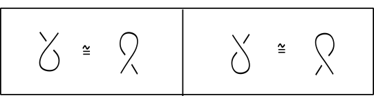
Refer to caption
Figure 6: The framing preserving relations in f​U​T​CfUTC.

Our motivation for Definition 2.10 is that quantum invariants are often not invariant under the first Reidemeister move, yet regular isotopy invariants can often be normalized to ambient isotopy invariants by a normalizing factor. On the other hand framed isotopy is needed in the construction of quantum invariants for framed knots.

3 The Extended Unoriented Tangloid Category

In this section we define an extended unoriented tangloid category, denoted 𝖳𝖺𝗇𝗀𝗂\mathsf{Tangi}. This category is obtained from U​T​CUTC by adding the empty generator ∅\emptyset to E⁡(β)E(\beta). For doing this, we first extend U​T​CUTC by auxilliary empty morphisms, ∅t\emptyset_{t} and ∅b\emptyset_{b}, acting as place-keepers at the top and bottom, for enabling to have every morphism from object nn to object nn for any nn. Diagrammatically, the place-keeper morphisms represent points.

3.1 Generating data for 𝖳𝖺𝗇𝗀𝗂\mathsf{Tangi} - the empty morphism

We now fix the generating data for the tangloid category 𝖳𝖺𝗇𝗀𝗂\mathsf{Tangi} (recall Subsection 2.2). Let

E(β)={X+,X−,∪,∩,¡,!,∅},E(\beta)=\{X_{+},X_{-},\cup,\cap,\,\text{¡},\mathord{!},\emptyset\},

As in U​T​CUTC, X±X_{\pm} represent positive/negative (classical) crossings, ∪,∩\cup,\cap are cup/cap, and ¡,!\text{¡},\mathord{!} are endpoint maps (head/leg in knotoid terminology). In 𝖳𝖺𝗇𝗀𝗂\mathsf{Tangi}, however, we would like each generator to have the same source and target. For this reason we extend U​T​CUTC to U​T​C​eUTCe by including the auxilliary top and bottom empty morphisms ∅t:1→0\emptyset_{t}\colon 1\to 0 and ∅b:0→1\emptyset_{b}\colon 0\to 1. These are represented diagrammatically as a top/bottom black dot ∙\bullet : [Uncaptioned image] and [Uncaptioned image], which act as placeholders for having every generator of 𝖳𝖺𝗇𝗀𝗂\mathsf{Tangi} acting from object 22 to object 22, except for !\mathord{!} and ¡ that now act from object 11 to object 11. So, the empty morphisms appear in the representations of all generators, except for the crossings. In other words we define in 𝖳𝖺𝗇𝗀𝗂\mathsf{Tangi},

∪: 2→2:=\displaystyle\cup\ \colon\ 2\to 2:= (∪∈UTC)∘(∅b⊗∅b)\displaystyle(\cup\in UTC)\circ(\emptyset_{b}\otimes\emptyset_{b})
∩: 2→2:=\displaystyle\cap\ \colon\ 2\to 2:= (∅t⊗∅t)∘(∩∈UTC)\displaystyle(\emptyset_{t}\otimes\emptyset_{t})\circ(\cap\in UTC)
¡: 1→1:=\displaystyle\text{¡}\ \colon\ 1\to 1:= ∅t∘(¡∈U​T​C)\displaystyle\emptyset_{t}\circ(\text{¡}\in UTC)
!: 1→1:=\displaystyle\mathord{!}\ \colon\ 1\to 1:= (!∈U​T​C)∘∅b\displaystyle(\mathord{!}\in UTC)\circ\emptyset_{b}

In the set of generators E⁡(β)E(\beta) of 𝖳𝖺𝗇𝗀𝗂\mathsf{Tangi} we further add the empty morphism

∅:=∅t∘∅b: 1→1\emptyset:=\emptyset_{t}\circ\emptyset_{b}\ \colon\ 1\to 1

represented diagrammatically as two corresponding black dots. In Figure 7 the elements of E⁡(β)E(\beta) are represented geometrically. Hence, the source and target objects for the generators of 𝖳𝖺𝗇𝗀𝗂\mathsf{Tangi} are now extended to the following:

δ1​X+\displaystyle\delta_{1}X_{+} =δ2​X+=2,\displaystyle=\delta_{2}X_{+}=2,
δ1​X−\displaystyle\delta_{1}X_{-} =δ2​X−=2,\displaystyle=\delta_{2}X_{-}=2,
δ1∪\displaystyle\delta_{1}\,\cup =δ2∪=2,\displaystyle=\delta_{2}\,\cup=2,
δ1∩\displaystyle\delta_{1}\,\cap =δ2∩=2,\displaystyle=\delta_{2}\,\cap=2,
δ1​¡\displaystyle\delta_{1}\,\text{¡} =δ2​¡=1,\displaystyle=\delta_{2}\,\text{¡}=1,
δ1​!\displaystyle\delta_{1}\,\mathord{!} =δ2​!=1,\displaystyle=\delta_{2}\,\mathord{!}=1,
δ1​∅\displaystyle\delta_{1}\,\emptyset =δ2​∅=1.\displaystyle=\delta_{2}\,\emptyset=1.
Refer to caption
Figure 7: Geometrical presentation of the 𝖳𝖺𝗇𝗀𝗂\mathsf{Tangi} generators.

3.2 Composition and tensoring rules for ∅\emptyset

Before providing the definition of 𝖳𝖺𝗇𝗀𝗂\mathsf{Tangi} we explain the composition and tensoring rules especially for ∅\emptyset in 𝖳𝖺𝗇𝗀𝗂\mathsf{Tangi}, as they arise from the general diagrammatic rules below.

  1. 1.

    When two arcs become incident they join and when two ∙\bullet’s become incident they merge into one, as for example in Figure 8 or Figure 12, and vice versa.

  2. 2.

    When two morphisms are composed, any isolated ∙\bullet in an interior region cancels, as for example in Figure 8. Conversely, an isolated ∙\bullet can emerge.

  3. 3.

    When two morphisms are composed, any arc that becomes incident with ∙\bullet is contracted to ∙\bullet, whether it is an arc of a cup/cap, crossing, or it contains an endpoint or not. See for example Figures 8 and 9.

  4. 4.

    For any morphism LL, the notation L⊗∅L\otimes\emptyset means that we tensor LL with ∅\emptyset by placing one ∙\bullet at the bottom right of LL and another corresponding ∙\bullet at the top right of LL. Analogously for the notation ∅⊗L\emptyset\otimes L.

Refer to caption
Figure 8: Contracting arcs and points
Refer to caption
Figure 9: Contracting arcs and endpoints
Notation 3.1.

As usual, for any n∈ℕ,n>1,n\in\mathbb{N},n>1, we adopt the notations idn:=id1⊗…⊗id1{\mathrm{id}}_{n}:={\mathrm{id}}_{1}\otimes\ldots\otimes{\mathrm{id}}_{1} and ∅n:=∅⊗…⊗∅\emptyset_{n}:=\emptyset\otimes\ldots\otimes\emptyset.

The above diagrammatic rules can be summarized in the following:

Definition 3.2.

For the ∅\emptyset in 𝖳𝖺𝗇𝗀𝗂\mathsf{Tangi} we have the following composition rules and tensoring rules.

  1. 1.

    ∅\emptyset composed with ∅\emptyset is contracted to ∅\emptyset: ∅∘∅=∅\emptyset\,\circ\emptyset=\emptyset. Generally, ∅n∘∅n=∅n\emptyset_{n}\,\circ\emptyset_{n}=\emptyset_{n}

  2. 2.

    id1{\mathrm{id}}_{1} composed with ∅\emptyset is contracted to ∅\emptyset: id1∘∅=∅=∅∘id1{\mathrm{id}}_{1}\,\circ\emptyset=\emptyset=\emptyset\,\circ{\mathrm{id}}_{1}

    Generally, idn∘∅n=∅n=∅n∘idn{\mathrm{id}}_{n}\,\circ\emptyset_{n}=\emptyset_{n}=\emptyset_{n}\,\circ{\mathrm{id}}_{n}

  3. 3.
    (∅⊗∅)∘∪\displaystyle(\emptyset\otimes\emptyset)\circ\,\cup =(∅⊗id1)∘∪=(id1⊗∅)∘∪=∅⊗∅\displaystyle=(\emptyset\otimes{\mathrm{id}}_{1})\,\circ\cup=({\mathrm{id}}_{1}\otimes\emptyset)\,\circ\cup=\emptyset\otimes\emptyset
    ∪∘(∅⊗∅)\displaystyle\ \cup\circ\,(\emptyset\otimes\emptyset)\, =∪∘(id1⊗∅)=∪∘(∅⊗id1)=∪\displaystyle=\cup\,\circ({\mathrm{id}}_{1}\otimes\emptyset)=\cup\,\circ(\emptyset\otimes{\mathrm{id}}_{1})=\cup
    ∪∘∪\displaystyle\cup\circ\cup =⁣∪\displaystyle=\cup
  4. 4.
    ∩∘(∅⊗∅)\displaystyle\cap\,\circ(\emptyset\otimes\emptyset) =∩∘(∅⊗id1)=∩∘(id1⊗∅)=∅⊗∅\displaystyle=\cap\,\circ(\emptyset\otimes{\mathrm{id}}_{1})=\cap\,\circ({\mathrm{id}}_{1}\otimes\emptyset)=\emptyset\otimes\emptyset
    (∅⊗∅)∘∩\displaystyle(\emptyset\otimes\emptyset)\,\circ\cap =(id1⊗∅)∘∩=(∅⊗id1)∘∩=∩\displaystyle=({\mathrm{id}}_{1}\otimes\emptyset)\,\circ\cap=(\emptyset\otimes{\mathrm{id}}_{1})\,\circ\cap=\cap
    ∩∘∩\displaystyle\cap\circ\cap =⁣∩\displaystyle=\cap
  5. 5.
    X±∘(∅⊗∅)\displaystyle X_{\pm}\,\circ(\emptyset\otimes\emptyset) =∅⊗∅=(∅⊗∅)∘X±\displaystyle=\emptyset\otimes\emptyset=(\emptyset\otimes\emptyset)\circ\,X_{\pm}
    (id1⊗∅)∘X+\displaystyle({\mathrm{id}}_{1}\otimes\emptyset)\,\circ X_{+} =(id1⊗∅)∘X−\displaystyle=({\mathrm{id}}_{1}\otimes\emptyset)\,\circ X_{-}
    (id1⊗∅)∘X+\displaystyle({\mathrm{id}}_{1}\otimes\emptyset)\,\circ X_{+} =X±∘(∅⊗id1)\displaystyle=X_{\pm}\,\circ(\emptyset\otimes{\mathrm{id}}_{1})
    (∅⊗id1)∘X+\displaystyle(\emptyset\otimes{\mathrm{id}}_{1})\circ\,X_{+} =(∅⊗id1)∘X−\displaystyle=(\emptyset\otimes{\mathrm{id}}_{1})\circ\,X_{-}
    (∅⊗id1)∘X+\displaystyle(\emptyset\otimes{\mathrm{id}}_{1})\circ\,X_{+} =X±∘(id1⊗∅)\displaystyle=X_{\pm}\circ({\mathrm{id}}_{1}\otimes\emptyset)
  6. 6.
    ¡∘∅\displaystyle\text{¡}\circ\emptyset =∅\displaystyle=\emptyset
    ∅∘¡\displaystyle\emptyset\circ\text{¡} =¡\displaystyle=\text{¡}
  7. 7.
    !∘∅\displaystyle!\circ\emptyset =!\displaystyle=\,\,!
    ∅∘!\displaystyle\emptyset\,\circ\,! =∅\displaystyle=\,\emptyset
  8. 8.
    (∅⊗¡)∘X+\displaystyle(\emptyset\otimes\text{¡})\circ X_{+} =(∅⊗¡)∘X−\displaystyle=(\emptyset\otimes\text{¡})\circ X_{-}
    (¡⊗∅)∘X+\displaystyle(\text{¡}\otimes\emptyset)\circ X_{+} =(¡⊗∅)∘X−\displaystyle=(\text{¡}\otimes\emptyset)\circ X_{-}
    X+∘(∅⊗¡)\displaystyle X_{+}\circ(\emptyset\otimes\text{¡}) =(∅⊗¡)=X−∘(∅⊗¡)\displaystyle=(\emptyset\otimes\text{¡})=X_{-}\circ(\emptyset\otimes\text{¡})
    X+∘(¡⊗∅)\displaystyle X_{+}\circ(\text{¡}\otimes\emptyset) =¡⊗∅=X−∘(¡⊗∅)\displaystyle=\text{¡}\otimes\emptyset=X_{-}\circ(\text{¡}\otimes\emptyset)
  9. 9.
    (∅⊗!)∘X+\displaystyle(\emptyset\,\otimes\,!)\circ X_{+} =(∅⊗!)=(∅⊗!)∘X−\displaystyle=(\emptyset\,\otimes\,!)=(\emptyset\,\otimes!)\circ X_{-}
    (!⊗∅)∘X+\displaystyle(!\otimes\emptyset)\circ X_{+} =(!⊗∅)=(!⊗∅)∘X−\displaystyle=(!\otimes\emptyset)\,=(!\otimes\emptyset)\circ X_{-}
    X+∘(∅⊗!)\displaystyle X_{+}\circ(\emptyset\,\otimes\,!) =X−∘(∅⊗!)\displaystyle=X_{-}\circ(\emptyset\,\otimes\,!)
    X+∘(!⊗∅)\displaystyle X_{+}\circ(!\otimes\emptyset) =X−∘(!⊗∅)\displaystyle=X_{-}\circ(!\otimes\emptyset)
  10. 10.
    (¡⊗∅)∘∪\displaystyle(\text{¡}\otimes\emptyset)\,\circ\cup =∅⊗∅=(∅⊗¡)∘∪\displaystyle=\emptyset\otimes\emptyset=(\emptyset\otimes\text{¡})\,\circ\cup
    ∪∘(!⊗∅)\displaystyle\cup\,\circ(!\otimes\emptyset) =∪=∪∘(∅⊗!)\displaystyle=\cup=\cup\,\circ(\emptyset\,\otimes!)
    (!⊗∅)∘∪\displaystyle(!\otimes\emptyset)\circ\cup\, =!⊗∅\displaystyle=\,!\otimes\emptyset
    (∅⊗!)∘∪\displaystyle(\emptyset\,\otimes\,!)\circ\cup =∅⊗!\displaystyle=\emptyset\,\otimes\,!
  11. 11.
    ∩∘(¡⊗∅)\displaystyle\cap\,\circ(\text{¡}\otimes\emptyset)\, =¡⊗∅\displaystyle=\text{¡}\otimes\emptyset
    ∩∘(∅⊗¡)\displaystyle\cap\,\circ(\emptyset\otimes\text{¡}) =∅⊗¡\displaystyle=\emptyset\,\otimes\text{¡}
    (¡⊗∅)∘∩\displaystyle(\text{¡}\otimes\emptyset)\,\circ\cap =∩=(∅⊗¡)∘∩\displaystyle=\cap=(\emptyset\otimes\text{¡})\,\circ\cap
    ∩∘(!⊗∅)\displaystyle\cap\,\circ(!\otimes\emptyset)\, =∅⊗∅=∩∘(∅⊗!)\displaystyle=\emptyset\otimes\emptyset=\cap\circ\,(\emptyset\otimes!)

3.3 The diagonal elements

The composition of a crossing with the placeholder morphism ∅\emptyset gives rise to two special elements in 𝖳𝖺𝗇𝗀𝗂\mathsf{Tangi}, the diagonal morphisms acting from object 22 to object 22, denoted by \\backslash and //, as illustrated in Figure 10:

\:=(id1⊗∅)∘X+and/:=(∅⊗id1)∘X+\backslash:=({\mathrm{id}}_{1}\otimes\emptyset)\circ X_{+}\quad\text{and}\quad/:=(\emptyset\otimes{\mathrm{id}}_{1})\circ X_{+}

These diagonal morphisms will subsequently appear as shorthand in the defining relations involving the generators.

Refer to caption
Figure 10: The diagonal morphisms \\backslash and //.

Note that, in the extension U​T​C​eUTCe of U​T​CUTC the diagonal elements can be obtained by tensoring the identity with ∅t\emptyset_{t} or ∅b\emptyset_{b} composed with cup-cap. For example,

\=(id1⊗∅t)∘(id1⊗∩)∘(∪⊗id1)∘(∅b⊗id1)\backslash=({\mathrm{id}}_{1}\otimes\emptyset_{t})\circ({\mathrm{id}}_{1}\otimes\cap)\circ(\cup\otimes{\mathrm{id}}_{1})\circ(\emptyset_{b}\otimes{\mathrm{id}}_{1})

For the diagonal elements we have the composition and tensoring rules below, which follow from the ones listed in Definition 3.2:

  1. 1.
    (/)∘(∅⊗∅)\displaystyle(/)\,\circ(\emptyset\otimes\emptyset) =∅⊗∅=(∅⊗∅)∘(/)\displaystyle=\emptyset\otimes\emptyset=(\emptyset\otimes\emptyset)\circ\,(/)
    (/)∘(∅⊗id1)\displaystyle(/)\,\circ(\emptyset\otimes{\mathrm{id}}_{1}) =∅⊗∅=(id1⊗∅)∘(/)\displaystyle=\emptyset\otimes\emptyset=({\mathrm{id}}_{1}\otimes\emptyset)\circ\,(/)
    (/)∘(id1⊗∅)\displaystyle(/)\,\circ({\mathrm{id}}_{1}\otimes\emptyset) =/=(∅⊗id1)∘(/)\displaystyle=/=(\emptyset\otimes{\mathrm{id}}_{1})\circ\,(/)
  2. 2.
    (\)∘(∅⊗∅)\displaystyle(\backslash)\,\circ(\emptyset\otimes\emptyset) =∅⊗∅=(∅⊗∅)∘(\)\displaystyle=\emptyset\otimes\emptyset=(\emptyset\otimes\emptyset)\circ\,(\backslash)
    (∅⊗id1)∘(\)\displaystyle(\emptyset\otimes{\mathrm{id}}_{1})\circ\,(\backslash) =∅⊗∅=(\)∘(id1⊗∅)\displaystyle=\emptyset\otimes\emptyset=(\backslash)\circ({\mathrm{id}}_{1}\otimes\emptyset)\,
    (id1⊗∅)∘(\)\displaystyle({\mathrm{id}}_{1}\otimes\emptyset)\,\circ(\backslash) =\=(\)∘(∅⊗id1)\displaystyle=\backslash=(\backslash)\circ\,(\emptyset\otimes{\mathrm{id}}_{1})\,\,
  3. 3.
    (∅⊗¡)∘(/)\displaystyle(\emptyset\otimes\text{¡})\,\circ(/) =(∅⊗¡)∘X+\displaystyle=(\emptyset\otimes\text{¡})\circ X_{+}
    (¡⊗∅)∘(\)\displaystyle(\text{¡}\otimes\emptyset)\circ\,(\backslash) =(¡⊗∅)∘X+\displaystyle=(\text{¡}\otimes\emptyset)\circ X_{+}
  4. 4.
    (\)∘(∅⊗!)\displaystyle(\backslash)\circ(\emptyset\,\otimes\,!) =X+∘(∅⊗!)\displaystyle=X_{+}\circ(\emptyset\,\otimes\,!)
    (/)∘(!⊗∅)\displaystyle(/)\circ(!\,\otimes\emptyset) =X+∘(!⊗∅)\displaystyle=X_{+}\circ(!\otimes\emptyset)
  5. 5.
    (¡⊗∅)∘(/)\displaystyle(\text{¡}\otimes\emptyset)\circ\,(/) =∅⊗∅=(∅⊗¡)∘(\)\displaystyle=\emptyset\otimes\emptyset=(\emptyset\otimes\text{¡})\,\circ(\backslash)
    (/)∘(¡⊗∅)\displaystyle(/)\,\circ(\text{¡}\otimes\emptyset) =¡⊗∅=(\)∘(¡⊗∅)\displaystyle=\text{¡}\otimes\emptyset=(\backslash)\,\circ(\text{¡}\otimes\emptyset)
    (/)∘(∅⊗¡)\displaystyle(/)\circ(\emptyset\otimes\text{¡}) =∅⊗¡=(\)∘(∅⊗¡)\displaystyle=\emptyset\otimes\text{¡}=(\backslash)\,\circ(\emptyset\otimes\text{¡})
  6. 6.
    (/)∘(∅⊗!)\displaystyle(/)\circ(\emptyset\,\otimes\,!) =∅⊗∅=(\)∘(!⊗∅)\displaystyle=\emptyset\,\otimes\emptyset=(\backslash)\circ(!\otimes\emptyset)
    (∅⊗!)∘(/)\displaystyle(\emptyset\,\otimes\,!)\,\circ(/) =∅⊗!=(∅⊗!)∘(\)\displaystyle=\emptyset\,\otimes\,!=(\emptyset\,\otimes\,!)\,\circ(\backslash)
    (!⊗∅)∘(\)\displaystyle(!\otimes\emptyset)\circ(\backslash) =!⊗∅=(!⊗∅)∘(/)\displaystyle=\,!\,\otimes\emptyset=(!\otimes\emptyset)\circ(/)
  7. 7.
    \∘X+\displaystyle\backslash\circ X_{+} =\∘/=\∘X−\displaystyle=\backslash\circ/=\backslash\circ X_{-}
    /∘X+\displaystyle/\circ X_{+} =/∘\=/∘X−\displaystyle=/\circ\backslash=/\circ X_{-}
    X+∘\\displaystyle X_{+}\circ\backslash =/∘\=X−∘\\displaystyle=/\circ\backslash=X_{-}\circ\backslash
    X+∘/\displaystyle X_{+}\circ/ =\∘/=X−∘/\displaystyle=\backslash\circ/=X_{-}\circ/
Refer to caption
Figure 11: Composing diagonal with crossing makes an arc tensored with ∅\emptyset.
Examples 3.3.

Here are some examples of morphisms in 𝖳𝖺𝗇𝗀𝗂\mathsf{Tangi}.

  1. 1.

    (∩⊗X+)∘(/⊗!⊗id1)∘(∩⊗¡⊗id1)∘(∩⊗X−)∘(X−⊗id2)∘(id1⊗X−⊗id1)(\cap\otimes X_{+})\circ(/\otimes\,!\otimes{\mathrm{id}}_{1})\circ(\cap\otimes\text{¡}\otimes{\mathrm{id}}_{1})\circ(\cap\otimes X_{-})\circ(X_{-}\otimes{\mathrm{id}}_{2})\circ({\mathrm{id}}_{1}\otimes X_{-}\otimes{\mathrm{id}}_{1}), see Figure 8.

  2. 2.

    (∩⊗id1)∘(\⊗id1)∘(id1⊗X+)∘(id1⊗X−)∘(X−⊗id1)∘(¡⊗id2)∘(∪⊗id1)(\cap\otimes{\mathrm{id}}_{1})\circ(\backslash\otimes{\mathrm{id}}_{1})\circ({\mathrm{id}}_{1}\otimes X_{+})\circ({\mathrm{id}}_{1}\otimes X_{-})\circ(X_{-}\otimes{\mathrm{id}}_{1})\circ(\text{¡}\otimes{\mathrm{id}}_{2})\circ(\cup\otimes{\mathrm{id}}_{1}), see Figure 9.

  3. 3.

    (id1⊗/⊗id1)∘(/⊗/)∘(id1⊗/⊗id1)({\mathrm{id}}_{1}\otimes/\otimes{\mathrm{id}}_{1})\circ(/\otimes/)\circ({\mathrm{id}}_{1}\otimes/\otimes{\mathrm{id}}_{1}), see Figure 12. This example can easily generalize to constructing morphisms depicted by any number of adjacent parallel straight arcs of any slope. See Figure 13. Such elements appear in relations [T4]−[T5]′[T_{4}]-[T_{5}]^{\prime} below.

Refer to caption
Figure 12: Creation of consecutive diagonals.
Refer to caption
Figure 13: Creation of consecutive diagonals.

3.4 Defining the extended unoriented tangloid category 𝖳𝖺𝗇𝗀𝗂\mathsf{Tangi}

We are now ready to define the extended unoriented tangloid category.

Definition 3.4 (Extended unoriented tangloid category).

Let Ω⁡(β)\Omega(\beta) be the free 12\tfrac{1}{2}–monoidal completion of the free path category P⁡(β∗)P(\beta^{*}) as defined in U​T​CUTC. The extended unoriented tangloid category, denoted by 𝖳𝖺𝗇𝗀𝗂\mathsf{Tangi}, is the strict monoidal category formally presented by

𝔉⁡(Ω⁡(β)/T¯¯),{\mathfrak{F}}\Big(\Omega(\beta)\big/\,\overline{\underline{T}}\Big),

where T¯¯\overline{\underline{T}} is the 12\tfrac{1}{2}–monoidal congruence generated by the local relations [Ti],[Ti]′[\mathrm{T}_{i}],[\mathrm{T}_{i}]^{\prime} listed below with all their variants and derivations, along with the composition rules for ∅\emptyset in Definition 3.2.

  • •

    [T1]:(∩)∘X−∼∩∼(∩)∘X+[T_{1}]:(\cap)\circ X_{-}\sim\cap\sim(\cap)\circ X_{+}

  • •

    [T1]′:(X−)∘∪∼∪∼(X+)∘∪[T_{1}]^{\prime}:(X_{-})\circ\cup\sim\cup\sim(X_{+})\circ\cup

  • •

    [T2]:(∩⊗id1)∘(id1⊗∪)∼(∅⊗/)∘(/⊗∅)[T_{2}]:(\cap\otimes\mathrm{id}_{1})\circ(\mathrm{id}_{1}\otimes\cup)\sim(\emptyset\otimes/)\circ(/\otimes\emptyset)

  • •

    [T2]′:(\⊗∅)∘(∅⊗\)∼(id1⊗∩)∘(∪⊗id1)[T_{2}]^{\prime}:(\backslash\otimes\emptyset)\circ(\emptyset\otimes\backslash)\sim(\mathrm{id}_{1}\otimes\cap)\circ(\cup\otimes\mathrm{id}_{1})

  • •

    [T3]:(\)∘(/)∼id1⊗∅[T_{3}]:(\backslash)\circ(/)\sim{\mathrm{id}}_{1}\otimes\emptyset

  • •

    [T3]′:∅⊗id1∼(/)∘(\)[T_{3}]^{\prime}:\emptyset\otimes{\mathrm{id}}_{1}\sim(/)\circ(\backslash)

  • •

    [T4]:(id⊗∩)∘((id2⊗\)∘(id1⊗\⊗id1)∘((id1⊗/⊗id1)∘(/⊗/)∘(id1⊗/⊗id1)))∼∩⊗∅[T_{4}]:({\mathrm{id}}\otimes\cap)\circ\Big(({\mathrm{id}}_{2}\otimes\backslash)\circ({\mathrm{id}}_{1}\otimes\backslash\otimes{\mathrm{id}}_{1})\circ\big(({\mathrm{id}}_{1}\otimes/\otimes{\mathrm{id}}_{1})\circ(/\otimes/)\circ({\mathrm{id}}_{1}\otimes/\otimes{\mathrm{id}}_{1})\big)\Big)\sim\cap\otimes\emptyset

  • •

    [T4]′:∅1⊗∩∼(∩⊗id1)∘((/⊗id2)∘(id1⊗/⊗id1)∘((id1⊗\⊗id1)∘(\⊗\)∘(id1⊗\⊗id1)))[T_{4}]^{\prime}:\emptyset_{1}\otimes\cap\sim\,(\cap\otimes{\mathrm{id}}_{1})\circ\Big((/\otimes{\mathrm{id}}_{2})\circ({\mathrm{id}}_{1}\otimes/\otimes{\mathrm{id}}_{1})\circ\big(({\mathrm{id}}_{1}\otimes\backslash\otimes{\mathrm{id}}_{1})\circ(\backslash\otimes\backslash)\circ({\mathrm{id}}_{1}\otimes\backslash\otimes{\mathrm{id}}_{1})\big)\Big)

  • •

    [T5]:((id2⊗\)∘(id1⊗\⊗id1)∘((id1⊗/⊗id1)∘(/⊗/)∘(id1⊗/⊗id1)))∘(∪⊗∅1)∼∅⊗∪[T_{5}]:\Big(({\mathrm{id}}_{2}\otimes\backslash)\circ({\mathrm{id}}_{1}\otimes\backslash\otimes{\mathrm{id}}_{1})\circ\big(({\mathrm{id}}_{1}\otimes/\otimes{\mathrm{id}}_{1})\circ(/\otimes/)\circ({\mathrm{id}}_{1}\otimes/\otimes{\mathrm{id}}_{1})\big)\Big)\circ(\cup\otimes\emptyset_{1})\sim\emptyset\otimes\cup

  • •

    [T5]′:∪⊗∅∼((/⊗id2)∘(id1⊗/⊗id1)∘((id1⊗\⊗id1)∘(\⊗\)∘(id1⊗\⊗id1)))∘(∅⊗∪)[T_{5}]^{\prime}:\cup\otimes\emptyset\sim\,\Big((/\otimes{\mathrm{id}}_{2})\circ({\mathrm{id}}_{1}\otimes/\otimes{\mathrm{id}}_{1})\circ\big(({\mathrm{id}}_{1}\otimes\backslash\otimes{\mathrm{id}}_{1})\circ(\backslash\otimes\backslash)\circ({\mathrm{id}}_{1}\otimes\backslash\otimes{\mathrm{id}}_{1})\big)\Big)\circ(\emptyset\otimes\cup)

  • •

    [T6]:X−∘X+∼id2∼X+∘X−[T_{6}]:X_{-}\circ X_{+}\sim\mathrm{id}_{2}\sim X_{+}\circ X_{-}

  • •

    [T7]:(X−⊗id1)∘(id1⊗X−)∘(X−⊗id1)∼(id1⊗X−)∘(X−⊗id1)∘(id1⊗X−)[T_{7}]:(X_{-}\otimes\mathrm{id}_{1})\circ(\mathrm{id}_{1}\otimes X_{-})\circ(X_{-}\otimes\mathrm{id}_{1})\sim(\mathrm{id}_{1}\otimes X_{-})\circ(X_{-}\otimes\mathrm{id}_{1})\circ(\mathrm{id}_{1}\otimes X_{-})

  • •

    [T8]:(∅⊗\)∘(∩⊗id1)∘(id1⊗X+)∼(/⊗∅)∘(id1⊗∩)∘(X−⊗id1)[T_{8}]:(\emptyset\otimes\backslash)\circ(\cap\otimes\mathrm{id}_{1})\circ(\mathrm{id}_{1}\otimes X_{+})\sim(/\otimes\emptyset)\circ(\mathrm{id}_{1}\otimes\cap)\circ(X_{-}\otimes\mathrm{id}_{1})

  • •

    [T8]′:(∅⊗\)∘(∩⊗id1)∘(id1⊗X−)∼(/⊗∅)∘(id1⊗∩)∘(X+⊗id1)[T_{8}]^{\prime}:(\emptyset\otimes\backslash)\circ(\cap\otimes{\mathrm{id}}_{1})\circ({\mathrm{id}}_{1}\otimes X_{-})\sim(/\otimes\emptyset)\circ({\mathrm{id}}_{1}\otimes\cap)\circ(X_{+}\otimes{\mathrm{id}}_{1})

  • •

    [T9]:(id1⊗X−)∘(∪⊗id1)∘(id1⊗/)∼(X+⊗id1)∘(id1⊗∪)∘(\⊗id1)[T_{9}]:({\mathrm{id}}_{1}\otimes X_{-})\circ(\cup\otimes{\mathrm{id}}_{1})\circ({\mathrm{id}}_{1}\otimes/)\sim(X_{+}\otimes{\mathrm{id}}_{1})\circ({\mathrm{id}}_{1}\otimes\cup)\circ(\backslash\otimes{\mathrm{id}}_{1})

  • •

    [T9]′:(id1⊗X+)∘(∪⊗id1)∘(id1⊗/)∼(X−⊗id1)∘(id1⊗∪)∘(\⊗id1)[T_{9}]^{\prime}:({\mathrm{id}}_{1}\otimes X_{+})\circ(\cup\otimes{\mathrm{id}}_{1})\circ({\mathrm{id}}_{1}\otimes/)\sim(X_{-}\otimes{\mathrm{id}}_{1})\circ({\mathrm{id}}_{1}\otimes\cup)\circ(\backslash\otimes{\mathrm{id}}_{1})

  • •

    [T10]:(\⊗id1)∘(id1⊗X+)∘(/⊗id1)∼(id1⊗/)∘(X+⊗id1)∘(id1⊗\)[T_{10}]:(\backslash\otimes{\mathrm{id}}_{1})\circ({\mathrm{id}}_{1}\otimes X_{+})\circ(/\otimes{\mathrm{id}}_{1})\sim({\mathrm{id}}_{1}\otimes/)\circ(X_{+}\otimes{\mathrm{id}}_{1})\circ({\mathrm{id}}_{1}\otimes\backslash)

  • •

    [T11]:(\⊗id1)∘(id1⊗X−)∘(/⊗id1)∼(id1⊗/)∘(X−⊗id1)∘(id1⊗\)[T_{11}]:(\backslash\otimes{\mathrm{id}}_{1})\circ({\mathrm{id}}_{1}\otimes X_{-})\circ(/\otimes{\mathrm{id}}_{1})\sim({\mathrm{id}}_{1}\otimes/)\circ(X_{-}\otimes{\mathrm{id}}_{1})\circ({\mathrm{id}}_{1}\otimes\backslash)

  • •

    [T12]:∩⊗∪∼∪∘∩∼∪⊗∩[T_{12}]:\cap\,\otimes\,\cup\sim\,\cup\circ\,\cap\sim\,\cup\otimes\,\cap

  • •

    [T13]:¡⊗!∼!∘¡∼!⊗¡[T_{13}]:\text{¡}\,\otimes\,!\sim\,!\circ\,\text{¡}\sim\,!\otimes\,\text{¡}

  • •

    [T14]:∩⊗!∼(∅⊗!)∘∩∼(!⊗∅)∘∩∼!⊗∩[T_{14}]:\cap\,\otimes\,!\sim\,(\emptyset\,\otimes\,!)\circ\,\cap\sim\,(!\,\otimes\,\emptyset)\circ\,\cap\sim\,!\otimes\,\cap

  • •

    [T14]′:¡⊗∪∼∪∘(∅⊗¡)∼∪∘(¡⊗∅)∘∪∼∪⊗¡[T_{14}]^{\prime}:\text{¡}\,\otimes\,\cup\sim\,\cup\circ(\emptyset\,\otimes\,\text{¡})\sim\,\cup\circ(\text{¡}\,\otimes\,\emptyset)\circ\,\cup\sim\,\cup\otimes\,\text{¡}

  • •

    [T15]:∩∘(id1⊗!)∼¡⊗∅[T_{15}]:\cap\circ(\mathrm{id}_{1}\otimes!)\sim\,\text{¡}\otimes\emptyset

  • •

    [T15]′:∅⊗¡∼∩∘(!⊗id1)[T_{15}]^{\prime}:\emptyset\otimes\,\text{¡}\sim\,\cap\circ(!\otimes\mathrm{id}_{1})

  • •

    [T16]:(id1⊗¡)∘∪∼!⊗∅[T_{16}]:(\mathrm{id}_{1}\otimes\text{¡})\circ\cup\sim\,\,!\otimes\emptyset

  • •

    [T16]′:∅⊗!∼(¡⊗id1)∘∪[T_{16}]^{\prime}:\emptyset\otimes\,!\sim(\text{¡}\otimes\mathrm{id}_{1})\circ\cup

  • •

    [T17]:(∅⊗¡)∘(/)∼¡⊗∅[T_{17}]:(\emptyset\otimes\text{¡})\circ(/)\sim\,\text{¡}\otimes\emptyset

  • •

    [T17]′:∅⊗¡∼(¡⊗∅)∘(\)[T_{17}]^{\prime}:\emptyset\otimes\,\text{¡}\sim\,(\text{¡}\otimes\emptyset)\circ(\backslash)

  • •

    [T18]:(\)∘(∅⊗!)∼!⊗∅[T_{18}]:(\backslash)\circ(\emptyset\,\otimes\,!)\sim\,\,!\,\otimes\,\emptyset

  • •

    [T18]′:∅⊗!∼(/)∘(!⊗∅)[T_{18}]^{\prime}:\emptyset\,\otimes\,!\sim\,(/)\circ(!\otimes\emptyset)

The above local relations can be presented diagrammatically as exemplified in Figure 14 (recall that we read the diagram from top to bottom), where the composition and tensoring rules also apply.

Refer to caption
Figure 14: Local relations in 𝖳𝖺𝗇𝗀𝗂\mathsf{Tangi}.

As in U​T​CUTC, it turns out that having the swing moves [T8]−[T9]′[T_{8}]-[T_{9}]^{\prime} in our list of isotopy moves makes redundant certain instances of Reidemeister moves involving horizontal arcs. But in 𝖳𝖺𝗇𝗀𝗂\mathsf{Tangi} we may need to compose with /,\/,\backslash in order to be able to apply the swing moves, as for example in the case of a horizontal RI move that can be obtained from a vertical one and two swing moves.

Also, as in U​T​CUTC, since 𝖳𝖺𝗇𝗀𝗂\mathsf{Tangi} is strict monoidal, we freely use the interchange law: for any composable morphisms f,f′,g,g′f,f^{\prime},g,g^{\prime} we have (f⊗g)∘(f′⊗g′)=(f∘f′)⊗(g∘g′)(f\otimes g)\circ(f^{\prime}\otimes g^{\prime})=(f\circ f^{\prime})\otimes(g\circ g^{\prime}). In particular, morphisms supported on disjoint tensor factors commute. For example, assuming composable identity morphisms we have:

(f⊗id)∘(id⊗g)=(f∘id)⊗(id∘g)=f⊗g=(id∘f)⊗(g∘id)=(id⊗g)∘(f⊗id)\displaystyle(f\otimes{\mathrm{id}})\circ({\mathrm{id}}\otimes g)=(f\circ{\mathrm{id}})\otimes({\mathrm{id}}\circ g)=f\otimes g=({\mathrm{id}}\circ f)\otimes(g\circ{\mathrm{id}})=({\mathrm{id}}\otimes g)\circ(f\otimes{\mathrm{id}}) (11)
[Uncaptioned image]

We do not list these “far-commuting” relations separately.

Remark 3.5.

Thanks to the interchange law and the identity morphism, we obtain the exchange of horizontal levels in the diagrammatic context. For instance, we obtain the exchange of horizontal levels of ∪\cup, ∩\cap or a crossing with an endpoint morphism (see Figure 15):

(∩⊗id)∘(id2⊗!)=(∩∘id2)⊗(id∘!)=(∩∘id2)⊗(!)=∩⊗!\displaystyle(\cap\otimes{\mathrm{id}})\circ({\mathrm{id}}_{2}\,\otimes\,!)=(\cap\circ{\mathrm{id}}_{2})\otimes({\mathrm{id}}\,\circ\,!)=(\cap\circ{\mathrm{id}}_{2})\otimes(\,!\,)=\cap\,\otimes\,! (12)
(id2⊗¡)∘(∪⊗id)=(id2∘∪)⊗(¡∘id)=(id2∘∪)⊗(¡)=∪⊗¡\displaystyle({\mathrm{id}}_{2}\,\otimes\text{¡}\,)\circ(\cup\otimes{\mathrm{id}})=({\mathrm{id}}_{2}\circ\cup)\otimes(\text{¡}\,\circ\,{\mathrm{id}})=({\mathrm{id}}_{2}\circ\cup)\otimes(\text{¡}\,)=\cup\,\otimes\,\text{¡} (13)
(X±⊗id)∘(id2⊗!)=(X±∘id2)⊗(id∘!)=(X±∘id2)⊗(!)=X±⊗!\displaystyle(X_{\pm}\otimes{\mathrm{id}})\circ({\mathrm{id}}_{2}\,\otimes\,!)=(X_{\pm}\circ{\mathrm{id}}_{2})\otimes({\mathrm{id}}\,\circ\,!)=(X_{\pm}\circ{\mathrm{id}}_{2})\otimes(\,!\,)=X_{\pm}\,\otimes\,! (14)

Note that Equation (10) in U​T​CUTC about horizontal shifts of endpoints also holds in 𝖳𝖺𝗇𝗀𝗂\mathsf{Tangi} by virtue of the more elementary relations [T17][T_{17}]–[T18]′[T_{18}]^{\prime} in 𝖳𝖺𝗇𝗀𝗂\mathsf{Tangi}.

Refer to caption
Figure 15: Geometric representations for the vertical shifts of endpoints.
Remark 3.6.

The vertical shifting of diagonals, showing in Figure 16, is obvious because:

\∘id2=id2∘\\backslash\circ{\mathrm{id}}_{2}={\mathrm{id}}_{2}\circ\backslash
/∘id2=id2∘//\circ{\mathrm{id}}_{2}={\mathrm{id}}_{2}\circ/
Refer to caption
Figure 16: Vertical shifting of diagonals.
Lemma 3.7.

The symmetric planar isotopy relations, which enable horizontal shifts of crossings with four or more ends can be derived from the basic [T10],[T11][T_{10}],[T_{11}] 𝖳𝖺𝗇𝗀𝗂\mathsf{Tangi} relations and the vertical shifting of diagonals. The relations with four ends is depicted in Figure 17 and reads as follows:

(\⊗id2)∘(id1⊗\⊗id1)∘(id2⊗X±)\displaystyle(\backslash\otimes{\mathrm{id}}_{2})\circ({\mathrm{id}}_{1}\otimes\backslash\otimes{\mathrm{id}}_{1})\circ({\mathrm{id}}_{2}\otimes X_{\pm}) ∘(id1⊗/⊗id1)∘(/⊗id2)\displaystyle\circ({\mathrm{id}}_{1}\otimes/\otimes{\mathrm{id}}_{1})\circ(/\otimes{\mathrm{id}}_{2})
=(\⊗/)∘(id1⊗X±⊗id1)∘(/⊗\)\displaystyle=(\backslash\otimes/)\circ({\mathrm{id}}_{1}\otimes X_{\pm}\otimes{\mathrm{id}}_{1})\circ(/\otimes\backslash)
=(id2⊗/)∘(id1⊗/⊗id1)∘(X±⊗id2)∘(id1⊗\⊗id1)∘(id2⊗\)\displaystyle=({\mathrm{id}}_{2}\otimes/)\circ({\mathrm{id}}_{1}\otimes/\otimes{\mathrm{id}}_{1})\circ(X_{\pm}\otimes{\mathrm{id}}_{2})\circ({\mathrm{id}}_{1}\otimes\backslash\otimes{\mathrm{id}}_{1})\circ({\mathrm{id}}_{2}\otimes\backslash)
Refer to caption
Figure 17: The horizontal shiftings of a crossing.
Proof.

We will prove the validity of the relations with four ends. The general case follows by an obvious iteration.

(\⊗/)∘(id1⊗X±⊗id1)∘(/⊗\)\displaystyle(\backslash\otimes/)\circ({\mathrm{id}}_{1}\otimes X_{\pm}\otimes{\mathrm{id}}_{1})\circ(/\otimes\backslash) =(\⊗/)∘(id2⊗id2)∘(id1⊗X±⊗id1)∘(id2⊗id2)∘(/⊗\)\displaystyle=(\backslash\otimes/)\circ({\mathrm{id}}_{2}\otimes{\mathrm{id}}_{2})\circ({\mathrm{id}}_{1}\otimes X_{\pm}\otimes{\mathrm{id}}_{1})\circ({\mathrm{id}}_{2}\otimes{\mathrm{id}}_{2})\circ(/\otimes\backslash)
=i​n​t​e​r​c​h​a​n​g​e​l​a​w(\∘id2)⊗(/∘id2)∘(id1⊗X±⊗id1)∘(id2∘/)⊗(id2∘\)\displaystyle\stackrel{{\scriptstyle interchange\,law}}{{=}}(\backslash\circ{\mathrm{id}}_{2})\otimes(/\circ{\mathrm{id}}_{2})\circ({\mathrm{id}}_{1}\otimes X_{\pm}\otimes{\mathrm{id}}_{1})\circ({\mathrm{id}}_{2}\circ/)\otimes({\mathrm{id}}_{2}\circ\backslash)
=R​e​m​a​r​k​3.6(\∘id2)⊗(id2∘/)∘(id1⊗X±⊗id1)∘(id2∘/)⊗(\∘id2)\displaystyle\stackrel{{\scriptstyle Remark~\ref{re:shifting of diagonal}}}{{=}}(\backslash\circ{\mathrm{id}}_{2})\otimes({\mathrm{id}}_{2}\circ/)\circ({\mathrm{id}}_{1}\otimes X_{\pm}\otimes{\mathrm{id}}_{1})\circ({\mathrm{id}}_{2}\circ/)\otimes(\backslash\circ{\mathrm{id}}_{2})
=i​n​t​e​r​c​h​a​n​g​e​l​a​w(\⊗id2)∘(id2⊗/)∘(id1⊗X±⊗id1)∘(id2⊗\)∘(/⊗id2)\displaystyle\stackrel{{\scriptstyle interchange\,law}}{{=}}(\backslash\otimes{\mathrm{id}}_{2})\circ({\mathrm{id}}_{2}\otimes/)\circ({\mathrm{id}}_{1}\otimes X_{\pm}\otimes{\mathrm{id}}_{1})\circ({\mathrm{id}}_{2}\otimes\backslash)\circ(/\otimes{\mathrm{id}}_{2})
=[T10](\⊗id2)∘(id1⊗\⊗id1)∘(id2⊗X±)∘(id1⊗/⊗id1)∘(/⊗id2)\displaystyle\stackrel{{\scriptstyle[T_{10}]}}{{=}}(\backslash\otimes{\mathrm{id}}_{2})\circ({\mathrm{id}}_{1}\otimes\backslash\otimes{\mathrm{id}}_{1})\circ({\mathrm{id}}_{2}\otimes X_{\pm})\circ({\mathrm{id}}_{1}\otimes/\otimes{\mathrm{id}}_{1})\circ(/\otimes{\mathrm{id}}_{2})
(\⊗/)∘(id1⊗X±⊗id1)∘(/⊗\)\displaystyle(\backslash\otimes/)\circ({\mathrm{id}}_{1}\otimes X_{\pm}\otimes{\mathrm{id}}_{1})\circ(/\otimes\backslash) =(\⊗/)∘(id2⊗id2)∘(id1⊗X±⊗id1)∘(id2⊗id2)∘(/⊗\)\displaystyle=(\backslash\otimes/)\circ({\mathrm{id}}_{2}\otimes{\mathrm{id}}_{2})\circ({\mathrm{id}}_{1}\otimes X_{\pm}\otimes{\mathrm{id}}_{1})\circ({\mathrm{id}}_{2}\otimes{\mathrm{id}}_{2})\circ(/\otimes\backslash)
=i​n​t​e​r​c​h​a​n​g​e​l​a​w(\∘id2)⊗(/∘id2)∘(id1⊗X±⊗id1)∘(id2∘/)⊗(id2∘\)\displaystyle\stackrel{{\scriptstyle interchange\,law}}{{=}}(\backslash\circ{\mathrm{id}}_{2})\otimes(/\circ{\mathrm{id}}_{2})\circ({\mathrm{id}}_{1}\otimes X_{\pm}\otimes{\mathrm{id}}_{1})\circ({\mathrm{id}}_{2}\circ/)\otimes({\mathrm{id}}_{2}\circ\backslash)
=R​e​m​a​r​k​3.6(id2∘\)⊗(/∘id2)∘(id1⊗X±⊗id1)∘(/∘id2)⊗(id2∘\)\displaystyle\stackrel{{\scriptstyle Remark~\ref{re:shifting of diagonal}}}{{=}}({\mathrm{id}}_{2}\circ\backslash)\otimes(/\circ{\mathrm{id}}_{2})\circ({\mathrm{id}}_{1}\otimes X_{\pm}\otimes{\mathrm{id}}_{1})\circ(/\circ{\mathrm{id}}_{2})\otimes({\mathrm{id}}_{2}\circ\backslash)
=i​n​t​e​r​c​h​a​n​g​e​l​a​w(id2⊗/)∘(\⊗id2)∘(id1⊗X±⊗id1)∘(/⊗id2)∘(id2⊗\)\displaystyle\stackrel{{\scriptstyle interchange\,law}}{{=}}({\mathrm{id}}_{2}\otimes/)\circ(\backslash\otimes{\mathrm{id}}_{2})\circ({\mathrm{id}}_{1}\otimes X_{\pm}\otimes{\mathrm{id}}_{1})\circ(/\otimes{\mathrm{id}}_{2})\circ({\mathrm{id}}_{2}\otimes\backslash)
=[T10](id2⊗/)∘(id1⊗/⊗id1)∘(X±⊗id2)∘(id1⊗\⊗id1)∘(id2⊗\)\displaystyle\stackrel{{\scriptstyle[T_{10}]}}{{=}}({\mathrm{id}}_{2}\otimes/)\circ({\mathrm{id}}_{1}\otimes/\otimes{\mathrm{id}}_{1})\circ(X_{\pm}\otimes{\mathrm{id}}_{2})\circ({\mathrm{id}}_{1}\otimes\backslash\otimes{\mathrm{id}}_{1})\circ({\mathrm{id}}_{2}\otimes\backslash)

∎

We conclude this section with the following definition in analogy to Definition 2.10 for U​T​CUTC.

Definition 3.8.

We define the regular extended unoriented tangloid category, denoted 𝗋𝖳𝖺𝗇𝗀𝗂\mathsf{rTangi}, to have the same generators and relations as 𝖳𝖺𝗇𝗀𝗂\mathsf{Tangi}, except for the relations [T1][T_{1}] and [T1]′[T_{1}]^{\prime} which are omitted. Furthermore, 𝖳𝖺𝗇𝗀𝗂\mathsf{Tangi} gives rise to the framed extended unoriented tangloid category, denoted 𝖿𝖳𝖺𝗇𝗀𝗂\mathsf{fTangi}, which has the same generators and relations as 𝖳𝖺𝗇𝗀𝗂\mathsf{Tangi}, except for the relations [T1][T_{1}] and [T1]′[T_{1}]^{\prime} which are replaced by the framing preserving relations depicted in Figure 18.

Refer to caption
Figure 18: The framing preserving relations in 𝖿𝖳𝖺𝗇𝗀𝗂\mathsf{fTangi}.

4 The Subcategory of Braidoids

In this subsection, we explain how the notion of braidoid, introduced by Gügümcü and Lambropoulou [10], can be interpreted inside the unoriented tangloid category U​T​CUTC and the extended unoriented tangloid category 𝖳𝖺𝗇𝗀𝗂\mathsf{Tangi} as a special class of morphisms forming a natural diagrammatic subcategory.

A braidoid diagram is a braid-like diagram drawn in the square I×I⊂ℝ2I\times I\subset\mathbb{R}^{2}, where I=[0,1]I=[0,1] and the vertical direction is in [10] oriented downward. It consists of a finite number of arcs, called strands, with only finitely many transversal double points, each equipped with over/under crossing data. As in classical braid diagrams, every strand is oriented downward and has no local maxima or minima; equivalently, each horizontal line intersects a strand at most once. The main difference from classical braid diagrams is that a braidoid diagram may contain free strands ending at two distinguished endpoints, called the leg and the head. The leg is the initial endpoint of a free strand, while the head is the terminal endpoint. The endpoints lying on the top and bottom boundary lines are called braidoid ends. These braidoid ends occur in corresponding pairs, one on the top boundary and one on the bottom boundary. Thus, a braidoid diagram generalizes a classical braid diagram by allowing two free strands with two special internal endpoints.

The isotopy classes of such diagrams under the allowed braidoid moves, are called braidoids. The allowed moves for braidoid diagrams are the downward-oriented Reidemeister moves Ω2\Omega_{2} and Ω3\Omega_{3}, planar Δ\Delta-moves respecting the monotonicity, and special moves of the endpoints called vertical moves and swing moves, which allow them to move within their diagrammatic region. However, as in knotoid theory, there are also forbidden moves: the leg or the head is not allowed to pass over or under another strand. These forbidden moves are essential, because allowing them would trivialize the braiding information carried by the free strands.

Braidoids can be realized inside U​T​CUTC and 𝖳𝖺𝗇𝗀𝗂\mathsf{Tangi} by restricting to those morphisms which are braid-like. More precisely,

Definition 4.1.

The braidoid category is defined as the subcategory 𝐁𝐫𝐝\mathbf{Brd} of U​T​CUTC with generating set {X+,X−,!,¡}\{X_{+},X_{-},!,\text{¡}\} and relations the set of relations of U​T​CUTC from which are excluded all relations involving the generators ∪,∩\cup,\cap.

Definition 4.2.

The extended braidoid category is defined as the subcategory

𝐁𝐫𝐝𝖳𝖺𝗇𝗀𝗂⊂𝖳𝖺𝗇𝗀𝗂\mathbf{Brd}_{\mathsf{Tangi}}\subset\mathsf{Tangi}

with generating set {X+,X−,!,¡,∅}\{X_{+},X_{-},!,\text{¡},\emptyset\} and relations the set of relations of 𝖳𝖺𝗇𝗀𝗂\mathsf{Tangi} from which are excluded all relations involving the generators ∪,∩\cup,\cap.

By Definitions 4.1 and 4.2, we have the inclusion functors

ι:𝐁𝐫𝐝↪U​T​Candι:𝐁𝐫𝐝𝖳𝖺𝗇𝗀𝗂↪𝖳𝖺𝗇𝗀𝗂.\iota:\mathbf{Brd}\hookrightarrow UTC\quad\mbox{and}\quad\iota:\mathbf{Brd}_{\mathsf{Tangi}}\hookrightarrow\mathsf{Tangi}.

The objects in 𝐁𝐫𝐝\mathbf{Brd} and 𝐁𝐫𝐝𝖳𝖺𝗇𝗀𝗂\mathbf{Brd}_{\mathsf{Tangi}} are natural numbers, interpreted geometrically as the number of boundary positions. The morphisms are those morphisms of U​T​CUTC resp. 𝖳𝖺𝗇𝗀𝗂\mathsf{Tangi} which can be represented by diagrams satisfying the definition of braidoid. Under this interpretation, the elementary pieces of a braidoid diagram are sent to the corresponding generators of 𝐁𝐫𝐝\mathbf{Brd} resp. 𝐁𝐫𝐝𝖳𝖺𝗇𝗀𝗂\mathbf{Brd}_{\mathsf{Tangi}} in the following way: the positive and negative braid crossings are represented by the crossing generators X+X_{+} and X−X_{-}:

σi+⟼idi−1⊗X+⊗idn−i−1\sigma_{i}^{+}\longmapsto{\mathrm{id}}_{i-1}\otimes X_{+}\otimes{\mathrm{id}}_{n-i-1}
σi−⟼idi−1⊗X−⊗idn−i−1\sigma_{i}^{-}\longmapsto{\mathrm{id}}_{i-1}\otimes X_{-}\otimes{\mathrm{id}}_{n-i-1}

The head and leg of a braidoid are represented by the endpoint generators ¡ and !! respectively:

hi⟼idi−1⊗!⊗idn−ih_{i}\longmapsto{\mathrm{id}}_{i-1}\otimes\,!\otimes{\mathrm{id}}_{n-i}
li⟼idi−1⊗¡⊗idn−il_{i}\longmapsto{\mathrm{id}}_{i-1}\otimes\,\text{¡}\otimes{\mathrm{id}}_{n-i}

The empty generator ∅\emptyset of 𝖳𝖺𝗇𝗀𝗂\mathsf{Tangi} plays the role of an implicit point or placeholder in the diagram allowing for the definition of a set of generators in the set of braidoids on nn strands under multiplication operation the concatenation (vertical stacking) of diagrams. It follows that the morphisms (including the generators) in 𝐁𝐫𝐝𝖳𝖺𝗇𝗀𝗂\mathbf{Brd}_{\mathsf{Tangi}} are in Hom⁡(n,n)\Hom(n,n), n∈ℕn\in{\mathbb{N}}.

The diagonal elements // and \\backslash shall be encoded as:

di⟼idi−1⊗/⊗idn−i−1d_{i}\longmapsto{\mathrm{id}}_{i-1}\otimes\,/\otimes{\mathrm{id}}_{n-i-1}
di¯⟼idi−1⊗\⊗idn−i−1\bar{d_{i}}\longmapsto{\mathrm{id}}_{i-1}\otimes\,\backslash\otimes{\mathrm{id}}_{n-i-1}

Vertical stacking of braidoid diagrams corresponds to categorical composition in 𝖳𝖺𝗇𝗀𝗂\mathsf{Tangi}, while horizontal juxtaposition corresponds to the tensor product. Therefore, the assignment from braidoid diagrams to U​T​CUTC-morphisms or 𝖳𝖺𝗇𝗀𝗂\mathsf{Tangi}-morphisms preserves both composition and tensor product. Furthermore, the relations in 𝐁𝐫𝐝\mathbf{Brd} and 𝐁𝐫𝐝𝖳𝖺𝗇𝗀𝗂\mathbf{Brd}_{\mathsf{Tangi}} correspond precisely to the isotopy relations in the set of braidoid diagrams. Hence, the categories 𝐁𝐫𝐝\mathbf{Brd} and 𝐁𝐫𝐝𝖳𝖺𝗇𝗀𝗂\mathbf{Brd}_{\mathsf{Tangi}} of braidoids may be regarded as the diagrammatic subcategories of U​T​CUTC and 𝖳𝖺𝗇𝗀𝗂\mathsf{Tangi} respectively, which furnish the natural categorical frameworks for the class of braidoids, and whose morphisms are monotone tangloid diagrams. In this sense, the extended tangloid category provides a larger ambient category, while braidoids are obtained by imposing the additional global condition that the diagrams are braid-like and by keeping the endpoint-forbidden moves excluded.

Remark 4.3.

The term ‘implicit point’ was introduced in [8, 7] as an auxiliary combinatorial structure in an attempt to express braidoids in terms of basic generating blocks. In [7] a systematic effort is made for listing basic relations among generating blocks of braidoids with operation the vertical stacking. Otherwise, the empty generators and the diagonal generators // and \\backslash were already introduced in the definition of the Motzkin algebra in [3].

Remark 4.4.

The categories U​T​CUTC and 𝖳𝖺𝗇𝗀𝗂\mathsf{Tangi} contain, as natural subcategories, the categories of knotoids, multi-knotoids, which are immersions of the unit interval and a number of circles in an oriented surface, and linkoids, immersions of some copies of the unit interval in an oriented surface. Thus, the tangloid framework provides new categorical models for these diagrammatic theories.

5 The Tangloid Algebra

The aim of this section is to define a tangloid algebra related to the extended unoriented tangloid category 𝖳𝖺𝗇𝗀𝗂\mathsf{Tangi} of Definition 3.4. Our construction is analogous in spirit to other diagrammatic settings where categorical morphisms give rise to natural endomorphism algebras; compare, for instance, the Brauer category framework in [16].

Definition 5.1 (Tangloid algebra 𝒯n\mathcal{T}_{n}).

Let 𝖳𝖺𝗇𝗀𝗂\mathsf{Tangi} be the extended tangloid category of Definition 3.4. For n≥0n\geq 0 the tangloid algebra of degree nn is defined as the ℂ\mathbb{C}–algebra

𝒯n:=ℂ​End𝖳𝖺𝗇𝗀𝗂​(n)\mathcal{T}_{n}\,:=\,{\mathbb{C}}\,\mathrm{End}_{{\mathsf{Tangi}}}(n)\,\

where

End𝖳𝖺𝗇𝗀𝗂​(n):=Hom𝖳𝖺𝗇𝗀𝗂⁡(n,n)\mathrm{End}_{{\mathsf{Tangi}}}(n):=\Hom_{\mathsf{Tangi}}(n,n)

The factor ℂ\mathbb{C} indicates the linearization of the endomorphism set End𝖳𝖺𝗇𝗀𝗂​(n)\mathrm{End}_{\mathsf{Tangi}}(n).

Equivalently we may state:

Proposition 5.2.

For each n≥0n\geq 0, the algebra 𝒯n=ℂ​End𝖳𝖺𝗇𝗀𝗂​(n)\mathcal{T}_{n}={\mathbb{C}}\,\mathrm{End}_{\mathsf{Tangi}}(n) is naturally identified with the unital diagram algebra over ℂ\mathbb{C} whose linear basis as a ℂ\mathbb{C}-vector space consists of all equivalence classes of tangloid diagrams in a rectangle with nn ordered boundary points on the top and nn on the bottom, some of which may merely act as placeholders, modulo the local relations of 𝖳𝖺𝗇𝗀𝗂\mathsf{Tangi} in Definition 3.4. Under this identification, the algebra multiplication uses the same rule as the composition rule for 𝖳𝖺𝗇𝗀𝗂\mathsf{Tangi}, induced by vertical stacking of diagrams (from top to bottom), addition is formal summation, and the unit, idn{\mathrm{id}}_{n}, is the identity diagram on nn vertical strands.

Proof.

By definition, End𝖳𝖺𝗇𝗀𝗂​(n)=Hom𝖳𝖺𝗇𝗀𝗂⁡(n,n)\mathrm{End}_{\mathsf{Tangi}}(n)=\Hom_{\mathsf{Tangi}}(n,n) is the set of morphisms from nn to nn in the extended tangloid category 𝖳𝖺𝗇𝗀𝗂\mathsf{Tangi}. Recall that, in the diagrammatic calculus underlying 𝖳𝖺𝗇𝗀𝗂\mathsf{Tangi}, cups, caps, endpoint maps and diagonal connectors create “empty” boundary positions (no arc emanating from that position). Since 𝖳𝖺𝗇𝗀𝗂\mathsf{Tangi} is presented diagrammatically, its morphisms are represented by tangloid diagrams modulo the defining local relations, which include the composition rules for one or more empty positions. By definition 𝒯n\mathcal{T}_{n} adopts all local relations of 𝖳𝖺𝗇𝗀𝗂\mathsf{Tangi}. Hence Hom𝖳𝖺𝗇𝗀𝗂⁡(n,n)\Hom_{\mathsf{Tangi}}(n,n) is precisely the set of n→nn\to n tangloid diagrams modulo these relations and is closed under composition. The multiplication in 𝒯n\mathcal{T}_{n} is the composition in 𝖳𝖺𝗇𝗀𝗂\mathsf{Tangi}, which is realized diagrammatically by vertical stacking (from top to bottom). The unit is the identity morphism, idn{\mathrm{id}}_{n}, represented by nn vertical strands. Passing to the ℂ\mathbb{C}-linear span ℂ​End𝖳𝖺𝗇𝗀𝗂​(n)\mathbb{C}\,\mathrm{End}_{\mathsf{Tangi}}(n) allows horizontal composition in the form of finite complex linear combinations of diagrams, giving the claimed vector space. ∎

The diagrams in 𝒯n\mathcal{T}_{n} are built from crossings, cups, caps, endpoint segments and empty positions. In 𝒯n\mathcal{T}_{n} we use the notations x,x¯,u,a,h,l,,ϕx,\bar{x},u,a,h,l,,\phi instead of X+,X−,∪,∩,,¡,!,∅X_{+},X_{-},\cup,\cap,,\text{¡},\mathord{!},\emptyset respectively, undergoing vertical composition. More precisely, in 𝒯n\mathcal{T}_{n} we distinguish the following elements, depicted in Figure 19:

  • •

    for 1≤i≤n−11\leq i\leq n-1, let xix_{i} (resp. x¯i\bar{x}_{i}) denote the positive (resp. negative) crossings, between the ii-th and (i+1)(i{+}1)-st strands;

  • •

    for 1≤i≤n−11\leq i\leq n-1, let uiu_{i} (resp. aia_{i}) denote the elementary cup (resp. cap) diagram connecting the top (resp. bottom) ii-th and (i+1)(i{+}1)-st boundary points (and all other strands vertical);

  • •

    for 1≤i≤n1\leq i\leq n, let hih_{i} (resp. lil_{i}) denote the diagram obtained by inserting the endpoint map ¡ (resp. !! ) at the ii-th position, with all other strands vertical.

  • •

    for 1≤i≤n1\leq i\leq n, let ϕi\phi_{i} denote the diagram obtained by inserting the empty set map (∅)(\emptyset) at the ii-th position, with all other strands vertical.

The elements xi,x¯i,ui,ai,hi,li,ϕix_{i},\bar{x}_{i},u_{i},a_{i},h_{i},l_{i},\phi_{i} generate 𝒯n\mathcal{T}_{n} as a ℂ\mathbb{C}–algebra. All generators except xi,x¯ix_{i},\bar{x}_{i} create boundary empty positions. The need for including ϕi\phi_{i} in the generators’ set arises from the fact that the tensoring operation in 𝖳𝖺𝗇𝗀𝗂\mathsf{Tangi} is not available in 𝒯n\mathcal{T}_{n}, as it does not preserve the degree nn.

Refer to caption
Figure 19: Geometric representatives of the tangloid algebra generators.

Note, as in 𝖳𝖺𝗇𝗀𝗂\mathsf{Tangi}, we use the following morphisms

  • •

    for 1≤i≤n−11\leq i\leq n-1, let did_{i} denote the diagonal connector diagram which joins (i,bottom)(i,\mathrm{bottom}) to (i+1,top)(i{+}1,\mathrm{top}) and all other strands vertical;

  • •

    for 1≤i≤n−11\leq i\leq n-1, let d¯i\bar{d}_{i} denote the diagonal connector diagram which joins (i+1,bottom)(i{+}1,\mathrm{bottom}) to (i,top)(i,\mathrm{top}) and all other strands vertical.

Although these diagonal morphisms are not generators, they can be obtained by composing a crossing with the placeholder morphism. We introduce the notation did_{i} and d¯i\bar{d}_{i} for these morphisms and use it to simplify the defining relations. See illustration in Figure 20.

Refer to caption
Figure 20: Diagonal morphisms in the tangloid algebra.

Definition 3.2 implies the following composition rules involving the generators ϕi\phi_{i}.

5.1 Composition rules involving the generators ϕi\phi_{i}

  1. 1.

    ϕi\phi_{i} composed with ϕi\phi_{i} is contracted to ϕi\phi_{i}: ϕi∘ϕi=ϕi\phi_{i}\,\circ\phi_{i}=\phi_{i}.

  2. 2.

    idn{\mathrm{id}}_{n} composed with ϕi\phi_{i} is contracted to ϕi\phi_{i}:

    idn∘ϕi=ϕi=ϕi∘idn\displaystyle{\mathrm{id}}_{n}\,\circ\phi_{i}=\phi_{i}=\phi_{i}\,\circ{\mathrm{id}}_{n}
  3. 3.
    (ϕi∘ϕi+1)∘ui\displaystyle(\phi_{i}\circ\phi_{i+1})\circ\,u_{i} =ϕi∘ui=ϕi+1∘ui=ϕi∘ϕi+1\displaystyle=\phi_{i}\,\circ u_{i}=\phi_{i+1}\,\circ u_{i}=\phi_{i}\circ\phi_{i+1}
    ui∘(ϕi∘ϕi+1)\displaystyle\ u_{i}\circ\,(\phi_{i}\circ\phi_{i+1})\, =ui∘ϕi=ui∘ϕi+1=ui\displaystyle=u_{i}\,\circ\phi_{i}=u_{i}\,\circ\phi_{i+1}=u_{i}
    ui∘ui\displaystyle u_{i}\circ u_{i} =ui\displaystyle=u_{i}
  4. 4.
    ai∘(ϕi∘ϕi+1)\displaystyle a_{i}\,\circ(\phi_{i}\circ\phi_{i+1}) =ai∘ϕi=ai∘(ϕi+1)=ϕi∘ϕi+1\displaystyle=a_{i}\,\circ\phi_{i}=a_{i}\,\circ(\phi_{i+1})=\phi_{i}\circ\phi_{i+1}
    (ϕi∘ϕi+1)∘ai\displaystyle(\phi_{i}\circ\phi_{i+1})\,\circ a_{i} =ϕi∘ai=ϕi+1∘ai=ai\displaystyle=\phi_{i}\,\circ a_{i}=\phi_{i+1}\,\circ a_{i}=a_{i}
    ai∘ai\displaystyle a_{i}\circ a_{i} =ai\displaystyle=a_{i}
  5. 5.
    xi∘(ϕi∘ϕi+1)\displaystyle x_{i}\,\circ(\phi_{i}\circ\phi_{i+1}) =(ϕi∘ϕi+1)=(ϕi∘ϕi+1)∘xi\displaystyle=(\phi_{i}\circ\phi_{i+1})=(\phi_{i}\circ\phi_{i+1})\circ\,x_{i}
    x¯i∘(ϕi∘ϕi+1)\displaystyle\bar{x}_{i}\,\circ(\phi_{i}\circ\phi_{i+1}) =(ϕi∘ϕi+1)=(ϕi∘ϕi+1)∘x¯i\displaystyle=(\phi_{i}\circ\phi_{i+1})=(\phi_{i}\circ\phi_{i+1})\circ\,\bar{x}_{i}
    ϕi+1∘xi\displaystyle\phi_{i+1}\circ x_{i} =ϕi+1∘x¯i\displaystyle=\phi_{i+1}\circ\bar{x}_{i}
    ϕi+1∘xi\displaystyle\phi_{i+1}\circ x_{i} =xi∘ϕi\displaystyle=x_{i}\circ\phi_{i}
    ϕi+1∘xi\displaystyle\phi_{i+1}\circ x_{i} =x¯i∘ϕi\displaystyle=\bar{x}_{i}\circ\phi_{i}
    ϕi∘xi\displaystyle\phi_{i}\circ\,x_{i} =ϕi∘x¯i\displaystyle=\phi_{i}\circ\,\bar{x}_{i}
    ϕi∘xi\displaystyle\phi_{i}\circ\,x_{i} =xi∘ϕi+1\displaystyle=x_{i}\circ\phi_{i+1}
    ϕi∘xi\displaystyle\phi_{i}\circ\,x_{i} =x¯i∘ϕi+1\displaystyle=\bar{x}_{i}\circ\phi_{i+1}
  6. 6.
    hi∘ϕi\displaystyle h_{i}\circ\phi_{i} =ϕi\displaystyle=\phi_{i}
    ϕi∘hi\displaystyle\phi_{i}\circ h_{i} =hi\displaystyle=h_{i}
  7. 7.
    li∘ϕi\displaystyle l_{i}\circ\phi_{i} =li\displaystyle=\,\,l_{i}
    ϕi∘li\displaystyle\phi_{i}\circ l_{i} =ϕi\displaystyle=\,\phi_{i}
  8. 8.
    (ϕi∘hi+1)∘xi\displaystyle(\phi_{i}\circ h_{i+1})\circ x_{i} =(ϕi∘hi+1)∘x¯i\displaystyle=(\phi_{i}\circ h_{i+1})\circ\bar{x}_{i}
    (hi∘ϕi+1)∘xi\displaystyle(h_{i}\circ\phi_{i+1})\circ x_{i} =(hi∘ϕi+1)∘x¯i\displaystyle=(h_{i}\circ\phi_{i+1})\circ\bar{x}_{i}
    xi∘(ϕi∘hi+1)\displaystyle x_{i}\circ(\phi_{i}\circ h_{i+1}) =(ϕi∘hi+1)=x¯i∘(ϕi∘hi+1)\displaystyle=(\phi_{i}\circ h_{i+1})=\bar{x}_{i}\circ(\phi_{i}\circ h_{i+1})
    xi∘(hi∘ϕi+1)\displaystyle x_{i}\circ(h_{i}\circ\phi_{i+1}) =hi∘ϕi+1=x¯i∘(hi∘ϕi+1)\displaystyle=h_{i}\circ\phi_{i+1}=\bar{x}_{i}\circ(h_{i}\circ\phi_{i+1})
  9. 9.
    (ϕi∘li+1)∘xi\displaystyle(\phi_{i}\,\circ l_{i+1})\circ x_{i} =(ϕi∘li+1)=(ϕi∘li+1)∘x¯i\displaystyle=(\phi_{i}\,\circ l_{i+1})=(\phi_{i}\,\circ l_{i+1})\circ\bar{x}_{i}
    (li∘ϕi+1)∘xi\displaystyle(l_{i}\circ\phi_{i+1})\circ x_{i} =(li∘ϕi+1)=(li∘ϕi+1)∘x¯i\displaystyle=(l_{i}\circ\phi_{i+1})\,=(l_{i}\circ\phi_{i+1})\circ\bar{x}_{i}
    xi∘(ϕi∘li+1)\displaystyle x_{i}\circ(\phi_{i}\,\circ l_{i+1}) =x¯i∘(ϕi∘li+1)\displaystyle=\bar{x}_{i}\circ(\phi_{i}\,\circ l_{i+1})
    xi∘(li∘ϕi+1)\displaystyle x_{i}\circ(l_{i}\circ\phi_{i+1}) =x¯i∘(li∘ϕi+1)\displaystyle=\bar{x}_{i}\circ(l_{i}\circ\phi_{i+1})
  10. 10.
    (hi∘ϕi+1)∘ui\displaystyle(h_{i}\circ\phi_{i+1})\,\circ u_{i} =(ϕi∘ϕi+1)=(ϕi∘hi+1)∘ui\displaystyle=(\phi_{i}\circ\phi_{i+1})=(\phi_{i}\circ h_{i+1})\circ u_{i}
    ui∘(li∘ϕi+1)\displaystyle u_{i}\,\circ(l_{i}\circ\phi_{i+1}) =ui=ui∘(ϕi∘li+1)\displaystyle=u_{i}=u_{i}\circ(\phi_{i}\,\circ l_{i+1})
    (li∘ϕi+1)∘ui\displaystyle(l_{i}\circ\phi_{i+1})\circ u_{i}\, =li∘ϕi+1\displaystyle=\,l_{i}\circ\phi_{i+1}
    (ϕi∘li+1)∘ui\displaystyle(\phi_{i}\,\circ l_{i+1})\circ u_{i} =ϕi∘li+1\displaystyle=\phi_{i}\,\circ l_{i+1}
  11. 11.
    ai∘(hi∘ϕi+1)\displaystyle a_{i}\,\circ(h_{i}\circ\phi_{i+1})\, =(hi∘ϕi+1)\displaystyle=(h_{i}\circ\phi_{i+1})
    ai∘(ϕi∘hi+1)\displaystyle a_{i}\,\circ(\phi_{i}\circ h_{i+1}) =(ϕi∘hi+1)\displaystyle=(\phi_{i}\circ h_{i+1})
    (hi∘ϕi+1)∘ai\displaystyle(h_{i}\circ\phi_{i+1})\,\circ a_{i} =ai=(ϕi∘hi+1)∘ai\displaystyle=a_{i}=(\phi_{i}\circ h_{i+1})\,\circ a_{i}
    ai∘(li∘ϕi+1)\displaystyle a_{i}\,\circ(l_{i}\circ\phi_{i+1})\, =ϕi∘ϕi+1=ai∘(ϕi∘li+1)\displaystyle=\phi_{i}\circ\phi_{i+1}=a_{i}\circ\,(\phi_{i}\,\circ l_{i+1})

5.2 The diagonal elements

For the diagonal elements we have the composition rules below, which follow from the ones listed in Subsection 5.1.

  1. 1.
    di∘(ϕi∘ϕi+1)\displaystyle d_{i}\,\circ(\phi_{i}\circ\phi_{i+1}) =(ϕi∘ϕi+1)=(ϕi∘ϕi+1)∘di\displaystyle=(\phi_{i}\circ\phi_{i+1})=(\phi_{i}\circ\phi_{i+1})\circ\,d_{i}
    di∘ϕi\displaystyle d_{i}\,\circ\phi_{i} =(ϕi∘ϕi+1)=ϕi+1∘di\displaystyle=(\phi_{i}\circ\phi_{i+1})=\phi_{i+1}\circ\,d_{i}
    di∘ϕi+1\displaystyle d_{i}\,\circ\phi_{i+1} =di=ϕi∘di\displaystyle=d_{i}=\phi_{i}\circ\,d_{i}
  2. 2.
    d¯i∘(ϕi∘ϕi+1)\displaystyle\bar{d}_{i}\,\circ(\phi_{i}\circ\phi_{i+1}) =ϕi∘ϕi+1=(ϕi∘ϕi+1)∘d¯i\displaystyle=\phi_{i}\circ\phi_{i+1}=(\phi_{i}\circ\phi_{i+1})\circ\,\bar{d}_{i}
    ϕi∘d¯i\displaystyle\phi_{i}\circ\,\bar{d}_{i} =ϕi∘ϕi+1=d¯i∘ϕi+1\displaystyle=\phi_{i}\circ\phi_{i+1}=\bar{d}_{i}\circ\phi_{i+1}\,
    ϕi+1∘d¯i\displaystyle\phi_{i+1}\,\circ\bar{d}_{i} =d¯i=d¯i∘ϕi\displaystyle=\bar{d}_{i}=\bar{d}_{i}\circ\,\phi_{i}\,\,
  3. 3.
    (ϕi∘hi+1)∘di\displaystyle(\phi_{i}\circ h_{i+1})\,\circ d_{i} =(ϕi∘hi+1)∘xi\displaystyle=(\phi_{i}\circ h_{i+1})\circ x_{i}
    (hi∘ϕi+1)∘d¯i\displaystyle(h_{i}\circ\phi_{i+1})\circ\,\bar{d}_{i} =(hi∘ϕi+1)∘xi\displaystyle=(h_{i}\circ\phi_{i+1})\circ x_{i}
  4. 4.
    d¯i∘(ϕi∘li+1)\displaystyle\bar{d}_{i}\circ(\phi_{i}\,\circ l_{i+1}) =xi∘(ϕi∘li+1)\displaystyle=x_{i}\circ(\phi_{i}\,\circ l_{i+1})
    di∘(li∘ϕi+1)\displaystyle d_{i}\circ(l_{i}\circ\phi_{i+1}) =xi∘(li∘ϕi+1)\displaystyle=x_{i}\circ(l_{i}\circ\phi_{i+1})
  5. 5.
    (hi∘ϕi+1)∘di\displaystyle(h_{i}\circ\phi_{i+1})\circ\,d_{i} =ϕi∘ϕi+1=(ϕi∘hi+1)∘d¯i\displaystyle=\phi_{i}\circ\phi_{i+1}=(\phi_{i}\circ h_{i+1})\,\circ\bar{d}_{i}
    di∘(hi∘ϕi+1)\displaystyle d_{i}\,\circ(h_{i}\circ\phi_{i+1}) =hi∘ϕi+1=d¯i∘(hi∘ϕi+1)\displaystyle=h_{i}\circ\phi_{i+1}=\bar{d}_{i}\,\circ(h_{i}\circ\phi_{i+1})
    di∘(ϕi∘hi+1)\displaystyle d_{i}\circ(\phi_{i}\circ h_{i+1}) =(ϕi∘hi+1)=d¯i∘(ϕi∘hi+1)\displaystyle=(\phi_{i}\circ h_{i+1})=\bar{d}_{i}\,\circ(\phi_{i}\circ h_{i+1})
  6. 6.
    di∘(ϕi∘li+1)\displaystyle d_{i}\circ(\phi_{i}\,\circ l_{i+1}) =(ϕi∘ϕi+1)=d¯i∘(li∘ϕi+1)\displaystyle=(\phi_{i}\circ\phi_{i+1})=\bar{d}_{i}\circ(l_{i}\circ\phi_{i+1})
    (ϕi∘li+1)∘di\displaystyle(\phi_{i}\,\circ l_{i+1})\,\circ d_{i} =(ϕi∘li+1)=(ϕi∘li+1)∘d¯i\displaystyle=(\phi_{i}\,\circ l_{i+1})=(\phi_{i}\,\circ l_{i+1})\,\circ\bar{d}_{i}
    (li∘ϕi+1)∘d¯i\displaystyle(l_{i}\circ\phi_{i+1})\circ\bar{d}_{i} =li∘ϕi+1=(li∘ϕi+1)∘di\displaystyle=l_{i}\circ\phi_{i+1}=(l_{i}\circ\phi_{i+1})\circ d_{i}
  7. 7.
    d¯i∘xi\displaystyle\bar{d}_{i}\circ x_{i} =d¯i∘di=d¯i∘x¯i\displaystyle=\bar{d}_{i}\circ d_{i}=\bar{d}_{i}\circ\bar{x}_{i}
    di∘xi\displaystyle d_{i}\circ x_{i} =di∘d¯i=di∘x¯i\displaystyle=d_{i}\circ\bar{d}_{i}=d_{i}\circ\bar{x}_{i}
    xi∘d¯i\displaystyle x_{i}\circ\bar{d}_{i} =di∘d¯i=x¯i∘d¯i\displaystyle=d_{i}\circ\bar{d}_{i}=\bar{x}_{i}\circ\bar{d}_{i}
    xi∘di\displaystyle x_{i}\circ d_{i} =d¯i∘di=x¯i∘di\displaystyle=\bar{d}_{i}\circ d_{i}=\bar{x}_{i}\circ d_{i}

The relations among the above generating elements are exactly those induced by the defining relations of 𝖳𝖺𝗇𝗀𝗂\mathsf{Tangi}. Hence, all relations in 𝒯n\mathcal{T}_{n} are understood as relations of local diagrams inside a fixed nn–box, with unused positions carrying vertical identities. See relations (𝒯1)−(𝒯18′)(\mathcal{T}^{1})-(\mathcal{T}^{18^{\prime}}) below. Moreover, a parameter δ∈ℂ\delta\in\mathbb{C} appears in the algebra δ​𝒯n\delta\mathcal{T}_{n}, Definition 7.1, when a closed circle is formed, when composing ai​uia_{i}u_{i}, or when the trivial knotoid is formed by the composition hi​lih_{i}l_{i}. See relations (𝒯19)−(𝒯20)(\mathcal{T}^{19})-(\mathcal{T}^{20}) below. More precisely, the relations in 𝒯n\mathcal{T}_{n} are:

ai∘x¯i\displaystyle a_{i}\circ\bar{x}_{i} =ai=ai∘xi,\displaystyle=a_{i}=a_{i}\circ x_{i}, 1≤i≤n−2\displaystyle 1\leq i\leq n-2 (𝒯1\mathcal{T}^{1})
x¯i∘ui\displaystyle\bar{x}_{i}\circ u_{i} =ui=xi∘ui,\displaystyle=u_{i}=x_{i}\circ u_{i}, 1≤i≤n−2\displaystyle 1\leq i\leq n-2 (𝒯1′\mathcal{T}^{1^{\prime}})
ai∘ui+1\displaystyle a_{i}\circ u_{i+1} =di+1∘di,\displaystyle=d_{i+1}\circ d_{i}, 1≤i≤n−2\displaystyle 1\leq i\leq n-2 (𝒯2\mathcal{T}^{2})
ai+1∘ui\displaystyle a_{i+1}\circ u_{i} =d¯i∘d¯i+1,\displaystyle=\bar{d}_{i}\circ\bar{d}_{i+1}, 1≤i≤n−2\displaystyle 1\leq i\leq n-2 (𝒯2′\mathcal{T}^{2^{\prime}})
d¯i∘di\displaystyle\bar{d}_{i}\circ d_{i} =ϕi+1,\displaystyle=\phi_{i+1}, 1≤i≤n−1\displaystyle 1\leq i\leq n-1 (𝒯3\mathcal{T}^{3})
di∘d¯i\displaystyle d_{i}\circ\bar{d}_{i} =ϕi,\displaystyle=\phi_{i}, 1≤i≤n−1\displaystyle 1\leq i\leq n-1 (𝒯3′\mathcal{T}^{3^{\prime}})
ai−1\displaystyle a_{i-1} =ai∘(d¯i+1∘d¯i∘di∘di−1∘di+1∘di),\displaystyle=a_{i}\circ(\bar{d}_{i+1}\circ\bar{d}_{i}\circ d_{i}\circ d_{i-1}\circ d_{i+1}\circ d_{i}), 1≤i≤n−1\displaystyle 1\leq i\leq n-1 (𝒯4\mathcal{T}^{4})
ai+1\displaystyle a_{i+1} =ai∘(di−1∘di∘d¯i∘d¯i−1∘d¯i+1∘d¯i),\displaystyle=a_{i}\circ(d_{i-1}\circ d_{i}\circ\bar{d}_{i}\circ\bar{d}_{i-1}\circ\bar{d}_{i+1}\circ\bar{d}_{i}), 1≤i≤n−1\displaystyle 1\leq i\leq n-1 (𝒯4′\mathcal{T}^{4^{\prime}})
ui\displaystyle u_{i} =(d¯i+1∘d¯i∘di∘di−1∘di+1∘di)∘ui−1\displaystyle=(\bar{d}_{i+1}\circ\bar{d}_{i}\circ d_{i}\circ d_{i-1}\circ d_{i+1}\circ d_{i})\circ u_{i-1} 1≤i≤n−1\displaystyle 1\leq i\leq n-1 (𝒯5\mathcal{T}^{5})
ui\displaystyle u_{i} =(di−1∘di∘d¯i∘d¯i−1∘d¯i+1∘d¯i)∘ui+1\displaystyle=(d_{i-1}\circ d_{i}\circ\bar{d}_{i}\circ\bar{d}_{i-1}\circ\bar{d}_{i+1}\circ\bar{d}_{i})\circ u_{i+1} 1≤i≤n−1\displaystyle 1\leq i\leq n-1 (𝒯5′\mathcal{T}^{5^{\prime}})
xi∘x¯i\displaystyle x_{i}\circ\bar{x}_{i} =idn=x¯i∘xi,\displaystyle={\mathrm{id}}_{n}=\bar{x}_{i}\circ x_{i}, 1≤i≤n−1\displaystyle 1\leq i\leq n-1 (𝒯6\mathcal{T}^{6})
x¯i∘x¯i+1∘x¯i\displaystyle\bar{x}_{i}\circ\bar{x}_{i+1}\circ\bar{x}_{i} =x¯i+1∘x¯i∘x¯i+1,\displaystyle=\bar{x}_{i+1}\circ\bar{x}_{i}\circ\bar{x}_{i+1}, 1≤i≤n−2\displaystyle 1\leq i\leq n-2 (𝒯7\mathcal{T}^{7})
d¯i+1∘ai∘xi+1\displaystyle\bar{d}_{i+1}\circ a_{i}\circ x_{i+1} =di∘ai+1∘x¯i,\displaystyle=d_{i}\circ a_{i+1}\circ\bar{x}_{i}, 1≤i≤n−2\displaystyle 1\leq i\leq n-2 (𝒯8\mathcal{T}^{8})
d¯i+1∘ai∘x¯i+1\displaystyle\bar{d}_{i+1}\circ a_{i}\circ\bar{x}_{i+1} =di∘ai+1∘xi,\displaystyle=d_{i}\circ a_{i+1}\circ x_{i}, 1≤i≤n−2\displaystyle 1\leq i\leq n-2 (𝒯8′\mathcal{T}^{8^{\prime}})
x¯i+1∘ui∘di+1\displaystyle\bar{x}_{i+1}\circ u_{i}\circ d_{i+1} =xi∘ui+1∘d¯i,\displaystyle=x_{i}\circ u_{i+1}\circ\bar{d}_{i}, 1≤i≤n−2\displaystyle 1\leq i\leq n-2 (𝒯9\mathcal{T}^{9})
x¯i+1∘ui∘di+1\displaystyle\bar{x}_{i+1}\circ u_{i}\circ d_{i+1} =xi∘ui+1∘d¯i,\displaystyle=x_{i}\circ u_{i+1}\circ\bar{d}_{i}, 1≤i≤n−2\displaystyle 1\leq i\leq n-2 (𝒯9′\mathcal{T}^{9^{\prime}})
d¯i∘xi+1∘di\displaystyle\bar{d}_{i}\circ x_{i+1}\circ d_{i} =di+1∘xi∘d¯i+1,\displaystyle=d_{i+1}\circ x_{i}\circ\bar{d}_{i+1}, 1≤i≤n−2\displaystyle 1\leq i\leq n-2 (𝒯10\mathcal{T}^{10})
d¯i∘x¯i+1∘di\displaystyle\bar{d}_{i}\circ\bar{x}_{i+1}\circ d_{i} =di+1∘x¯i∘d¯i+1,\displaystyle=d_{i+1}\circ\bar{x}_{i}\circ\bar{d}_{i+1}, 1≤i≤n−2\displaystyle 1\leq i\leq n-2 (𝒯11\mathcal{T}^{11})
ui+1∘ai\displaystyle u_{i+1}\circ a_{i} =ui∘ai=ui∘ai+2,\displaystyle=u_{i}\circ a_{i}=u_{i}\circ a_{i+2}, 1≤i≤n−1\displaystyle 1\leq i\leq n-1 (𝒯12\mathcal{T}^{12})
hi∘li+1\displaystyle h_{i}\circ l_{i+1} =li∘hi=li∘hi+1,\displaystyle=l_{i}\circ h_{i}=l_{i}\circ h_{i+1}, 1≤i≤n−1\displaystyle 1\leq i\leq n-1 (𝒯13\mathcal{T}^{13})
li+2∘ai\displaystyle l_{i+2}\circ a_{i} =li+1∘ai=li∘ai=li∘ai+1,\displaystyle=l_{i+1}\circ a_{i}=l_{i}\circ a_{i}=l_{i}\circ a_{i+1}, 1≤i≤n−1\displaystyle 1\leq i\leq n-1 (𝒯14\mathcal{T}^{14})
ui+1∘hi\displaystyle u_{i+1}\circ h_{i} =ui∘hi+1=ui∘hi=ui∘hi+2,\displaystyle=u_{i}\circ h_{i+1}=u_{i}\circ h_{i}=u_{i}\circ h_{i+2}, 1≤i≤n−1\displaystyle 1\leq i\leq n-1 (𝒯14′\mathcal{T}^{14^{\prime}})
ai∘li\displaystyle a_{i}\circ l_{i} =hi+1,\displaystyle=h_{i+1}, 1≤i≤n−1\displaystyle 1\leq i\leq n-1 (𝒯15\mathcal{T}^{15})
ai∘li+1\displaystyle a_{i}\circ l_{i+1} =hi,\displaystyle=h_{i}, 1≤i≤n−1\displaystyle 1\leq i\leq n-1 (𝒯15′\mathcal{T}^{15^{\prime}})
hi∘ui\displaystyle h_{i}\circ u_{i} =li+1,\displaystyle=l_{i+1}, 1≤i≤n−1\displaystyle 1\leq i\leq n-1 (𝒯16\mathcal{T}^{16})
hi+1∘ui\displaystyle h_{i+1}\circ u_{i} =li,\displaystyle=l_{i}, 1≤i≤n−1\displaystyle 1\leq i\leq n-1 (𝒯16′\mathcal{T}^{16^{\prime}})
hi+1∘di\displaystyle h_{i+1}\circ d_{i} =hi,\displaystyle=h_{i}, 1≤i≤n−1\displaystyle 1\leq i\leq n-1 (𝒯17\mathcal{T}^{17})
hi∘d¯i\displaystyle h_{i}\circ\bar{d}_{i} =hi+1,\displaystyle=h_{i+1}, 1≤i≤n−1\displaystyle 1\leq i\leq n-1 (𝒯17′\mathcal{T}^{17^{\prime}})
d¯i∘li+1\displaystyle\bar{d}_{i}\circ l_{i+1} =li,\displaystyle=l_{i}, 1≤i≤n−1\displaystyle 1\leq i\leq n-1 (𝒯18\mathcal{T}^{18})
di∘li\displaystyle d_{i}\circ l_{i} =li+1,\displaystyle=l_{i+1}, 1≤i≤n−1\displaystyle 1\leq i\leq n-1 (𝒯18′\mathcal{T}^{18^{\prime}})

extended by the following extra relations in δ​𝒯n\delta\mathcal{T}_{n}:

ai∘ui\displaystyle a_{i}\circ u_{i} =δ​ϕi∘ϕi+1,\displaystyle=\delta\,\phi_{i}\circ\phi_{i+1}, 1≤i≤n−1\displaystyle 1\leq i\leq n-1 (𝒯19\mathcal{T}^{19})
hi∘li\displaystyle h_{i}\,\circ l_{i} =δ​ϕi\displaystyle=\delta\,\phi_{i} 1≤i≤n\displaystyle 1\leq i\leq n (𝒯20\mathcal{T}^{20})

Far commuting for disjoint support: Whenever two generators act on disjoint tensor blocks (e.g. |i−j|>1|i-j|>1 for two-strand generators), they commute; we do not list these relations separately.

Definition 5.3.

We call the tangloid algebra 𝒯n\mathcal{T}_{n} regular tangloid algebra, denoted r​𝒯nr\mathcal{T}_{n}, to have the same definition as the tangloid algebra 𝒯n\mathcal{T}_{n}, but with the relations (𝒯1)(\mathcal{T}^{1}) and (𝒯1′)(\mathcal{T}^{1^{\prime}}) omitted. Furthermore, 𝒯n\mathcal{T}_{n} gives rise to the framed tangloid category, denoted f​𝒯nf\mathcal{T}_{n}, having the same definition as 𝒯n\mathcal{T}_{n}, except for relations (𝒯1)(\mathcal{T}^{1}) and (𝒯1′)(\mathcal{T}^{1^{\prime}}) which are replaced by the framing preserving relations depicted in Figure 18.

6 The Algebra of Braidoids

We define the braidoid algebra ℬn\mathcal{B}_{n} related to the extended braidoid category 𝐁𝐫𝐝𝖳𝖺𝗇𝗀𝗂⊂𝖳𝖺𝗇𝗀𝗂\mathbf{Brd}_{\mathsf{Tangi}}\subset\mathsf{Tangi} of Definition 4.2. The braidoid algebra ℬn\mathcal{B}_{n} provides an algebraic structure in the set of braidoids, sought in [8, 7], filling thus a gap in the literature.

Definition 6.1 (Braidoid algebra ℬn\mathcal{B}_{n}).

For n≥0n\geq 0 the braidoid algebra of degree nn is defined as the ℂ\mathbb{C}–algebra

ℬn:=ℂ​End𝐁𝐫𝐝𝖳𝖺𝗇𝗀𝗂​(n)\mathcal{B}_{n}\,:=\,{\mathbb{C}}\,\mathrm{End}_{\mathbf{Brd}_{\mathsf{Tangi}}}(n)\,\

where

End𝐁𝐫𝐝𝖳𝖺𝗇𝗀𝗂​(n):=Hom𝐁𝐫𝐝𝖳𝖺𝗇𝗀𝗂⁡(n,n).\mathrm{End}_{\mathbf{Brd}_{\mathsf{Tangi}}}(n):=\Hom_{\mathbf{Brd}_{\mathsf{Tangi}}}(n,n).

It follows that ℬn\mathcal{B}_{n} has as generators: xix_{i} (resp. x¯i\bar{x}_{i}) corresponding to the positive (resp. negative) crossings for 1≤i≤n−11\leq i\leq n-1, hih_{i} and lil_{i} the head and leg endpoints at the iith position, with all other strands vertical, for 1≤i≤n1\leq i\leq n, and the diagrams obtained by inserting the empty set map (∅)(\emptyset) at the ii-th position, ϕi\phi_{i}, with all other strands vertical, for 1≤i≤n1\leq i\leq n.

ℬn\mathcal{B}_{n} also includes the diagonal connectors did_{i} joining (i,bottom)(i,\mathrm{bottom}) to (i+1,top)(i{+}1,\mathrm{top}) with all other strands vertical, and d¯i\bar{d}_{i} joining (i+1,bottom)(i{+}1,\mathrm{bottom}) to (i,top)(i,\mathrm{top}) with all other strands vertical, which are elements of special interest. These elements are subjected to the composition rules involving the generators ϕi\phi_{i} listed in Subsection 5.1, excluding (3), (4), (10), (11), which involve the elements uiu_{i} and aia_{i}, and relations of the tangloid algebra 𝒯n\mathcal{T}_{n} which do not contain the generators uiu_{i} and aia_{i}. For completeness we list the relations below:

d¯i∘di\displaystyle\bar{d}_{i}\circ d_{i} =ϕi+1,\displaystyle=\phi_{i+1}, 1≤i≤n−1\displaystyle 1\leq i\leq n-1 (𝒯3\mathcal{T}^{3})
di∘d¯i\displaystyle d_{i}\circ\bar{d}_{i} =ϕi,\displaystyle=\phi_{i}, 1≤i≤n−1\displaystyle 1\leq i\leq n-1 (𝒯3′\mathcal{T}^{3^{\prime}})
xi∘x¯i\displaystyle x_{i}\circ\bar{x}_{i} =idn=x¯i∘xi,\displaystyle={\mathrm{id}}_{n}=\bar{x}_{i}\circ x_{i}, 1≤i≤n−1\displaystyle 1\leq i\leq n-1 (𝒯6\mathcal{T}^{6})
x¯i∘x¯i+1∘x¯i\displaystyle\bar{x}_{i}\circ\bar{x}_{i+1}\circ\bar{x}_{i} =x¯i+1∘x¯i∘x¯i+1,\displaystyle=\bar{x}_{i+1}\circ\bar{x}_{i}\circ\bar{x}_{i+1}, 1≤i≤n−2\displaystyle 1\leq i\leq n-2 (𝒯7\mathcal{T}^{7})
d¯i∘xi+1∘di\displaystyle\bar{d}_{i}\circ x_{i+1}\circ d_{i} =di+1∘xi∘d¯i+1,\displaystyle=d_{i+1}\circ x_{i}\circ\bar{d}_{i+1}, 1≤i≤n−2\displaystyle 1\leq i\leq n-2 (𝒯10\mathcal{T}^{10})
d¯i∘x¯i+1∘di\displaystyle\bar{d}_{i}\circ\bar{x}_{i+1}\circ d_{i} =di+1∘x¯i∘d¯i+1,\displaystyle=d_{i+1}\circ\bar{x}_{i}\circ\bar{d}_{i+1}, 1≤i≤n−2\displaystyle 1\leq i\leq n-2 (𝒯11\mathcal{T}^{11})
hi∘li+1\displaystyle h_{i}\circ l_{i+1} =li∘hi=li∘hi+1,\displaystyle=l_{i}\circ h_{i}=l_{i}\circ h_{i+1}, 1≤i≤n−1\displaystyle 1\leq i\leq n-1 (𝒯13\mathcal{T}^{13})
hi+1∘di\displaystyle h_{i+1}\circ d_{i} =hi,\displaystyle=h_{i}, 1≤i≤n−1\displaystyle 1\leq i\leq n-1 (𝒯17\mathcal{T}^{17})
hi∘d¯i\displaystyle h_{i}\circ\bar{d}_{i} =hi+1,\displaystyle=h_{i+1}, 1≤i≤n−1\displaystyle 1\leq i\leq n-1 (𝒯17′\mathcal{T}^{17^{\prime}})
d¯i∘li+1\displaystyle\bar{d}_{i}\circ l_{i+1} =li,\displaystyle=l_{i}, 1≤i≤n−1\displaystyle 1\leq i\leq n-1 (𝒯18\mathcal{T}^{18})
di∘li\displaystyle d_{i}\circ l_{i} =li+1,\displaystyle=l_{i+1}, 1≤i≤n−1\displaystyle 1\leq i\leq n-1 (𝒯18′\mathcal{T}^{18^{\prime}})
Remark 6.2.

Elements in the braidoid algebra arising as compositions of generators are not necessarily braidoids in the geometric sense. On the other hand any braidoid can be expressed as a composition of the generators of the braidoid algebra. Our construction provides an extended algebraic framework for expressing geometric braidoids.

Remark 6.3.

There is a natural analogy between the braidoid framework and the inverse braid monoid I​BnIB_{n} of Easdown and Lavers [5]. The latter extends the braid group by allowing strands of a braid to be deleted, so that its elements are represented by partial braids. In the braidoid setting, partiality arises diagrammatically by strands with interior endpoints. Thus, at the diagrammatic level, braidoids may be regarded as an endpoint-enhanced extension of the partial-braid viewpoint underlying the inverse braid monoid. After linearisation, this analogy passes to the algebraic level: the braidoid subalgebra of 𝒯n\mathcal{T}_{n} may be compared with the monoid algebra ℂ⁡[I​Bn]\mathbb{C}[IB_{n}]. A precise relationship between these two algebras, including the existence of natural homomorphisms or embeddings, is left for future investigation.

We conclude the section with a comparison with the study in [8, 7].

Remark 6.4.

In [8, 7] the placeholders are called ‘implicit points’ and generators are referred to as elementary blocks. The set of elementary blocks include the shifting blocks, corresponding to our diagonal elements, and identity elements with an empty vertical position (placeholder). But these last elements can arise from composition of diagonal elements di​d¯id_{i}\bar{d}_{i} and di​d¯id_{i}\bar{d}_{i}. Furthermore, in the composition rules in [8, 7], usual ends can be concatenated with only usual ends at the same position so that the resulting diagram contains strands stretching from top to bottom row. All relations listed in [7] are included in the relations of our braidoid algebra. For example, we can write relation 12 in [7] as d¯i∘d¯i+1∘xi+2∘di+1​di=d¯i∘di+2∘xi+1∘di∘d¯i+2\bar{d}_{i}\circ\bar{d}_{i+1}\circ x_{i+2}\circ d_{i+1}d_{i}=\bar{d}_{i}\circ d_{i+2}\circ x_{i+1}\circ d_{i}\circ\bar{d}_{i+2}, and relation 13 as d¯i∘d¯i+1∘xi+2∘di+1​di=di+2∘di+1∘xi∘d¯i+1∘d¯i+2\bar{d}_{i}\circ\bar{d}_{i+1}\circ x_{i+2}\circ d_{i+1}d_{i}=d_{i+2}\circ d_{i+1}\circ x_{i}\circ\bar{d}_{i+1}\circ\bar{d}_{i+2}. Our construction ensures that we have obtained a full set of relations. Finally, we point out a misprint in relations 5 in [7]: σi±1​lj=lj​(σi(j))±1\sigma_{i}^{\pm 1}\,l_{j}=l_{j}\,\bigl(\sigma_{i}^{(j)}\bigr)^{\pm 1}. The correct one is:

(σi(j))±1​lj=lj​σi±1,fori+2≤j≤kor​ 1≤j≤i−1.\bigl(\sigma_{i}^{(j)}\bigr)^{\pm 1}\,l_{j}=l_{j}\,\sigma_{i}^{\pm 1},\qquad\text{for}\ \ i+2\leq j\leq k\ \ \text{or}\ \ 1\leq j\leq i-1.

7 A diagrammatic bilinear form in the reduced tangloid algebra

In this section we define the standard diagrammatic pairing on the reduced tangloid algebra δ​𝒯n\delta\mathcal{T}_{n}.

Definition 7.1 (Reduced tangloid algebra 𝒯n\mathcal{T}_{n}).

We define the reduced tangloid algebra of degree nn, δ​𝒯n\mathcal{\delta T}_{n}, as the quotient of 𝒯n\mathcal{T}_{n} under the extra relations where a parameter δ∈ℂ\delta\in\mathbb{C} appears when a closed circle is formed, when composing ai​uia_{i}u_{i}, or when the trivial knotoid is formed by the composition hi​lih_{i}l_{i}.

By Proposition 5.2, δ​𝒯n\delta\mathcal{T}_{n} can be identified with the ℂ{\mathbb{C}}–linear span of all equivalence classes of tangloid diagrams n→nn\to n, where some points may be placeholders, representing endomorphisms n→nn\to n, modulo the extra reduced relations.

7.1 The reflection anti-involution

Let ∗:δ​𝒯n→δ​𝒯n*\colon\delta\mathcal{T}_{n}\to\delta\mathcal{T}_{n} denote the vertical reflection of diagrams in the horizontal axis of the rectangle. Since we are in the endomorphism algebra End𝖳𝖺𝗇𝗀𝗂⁡(n)\mathrm{End}_{{\mathsf{Tangi}}(n)}, reflection preserves the object nn and hence induces a ℂ{\mathbb{C}}–linear map on δ​𝒯n\delta\mathcal{T}_{n}.

Lemma 7.2 (Anti-involution).

The reflection map ∗* is an involutive anti-automorphism:

(a​b)∗=b∗​a∗,(id)∗=id,(m∗)∗=m(ab)^{*}=b^{*}a^{*},\qquad({\mathrm{id}})^{*}={\mathrm{id}},\qquad(m^{*})^{*}=m

for a,b,m∈δ​𝒯na,b,m\in\delta\mathcal{T}_{n}.

Proof.

On the distinguished generators of Definition 5.1 one has

(xi)∗=x¯i,(x¯i)∗=xi,(ui)∗=ai,(ai)∗=ui,(x_{i})^{*}=\bar{x}_{i},\qquad(\bar{x}_{i})^{*}=x_{i},\qquad(u_{i})^{*}=a_{i},\qquad(a_{i})^{*}=u_{i},
(hi)∗=li,(li)∗=hi,(ϕi)∗=ϕi(h_{i})^{*}=l_{i},\qquad(l_{i})^{*}=h_{i},\qquad(\phi_{i})^{*}=\phi_{i}

and ∗* extends multiplicatively by swapping factors and ℂ{\mathbb{C}}–linearly to all of δ​𝒯n\delta\mathcal{T}_{n}. ∎

Definition 7.3 (Loop count).

For a diagram D∈δ​𝒯nD\in\delta\mathcal{T}_{n}, let κ⁡(D)\kappa(D) be the number of simple closed components 0→00\to 0 (forgetting the placeholders), including the trivial knotoid, that appear when simplifying DD using the defining relations of δ​𝒯n\delta\mathcal{T}_{n}, so that each such component contributes a scalar factor δ∈ℂ\delta\in\mathbb{C}. So, δκ⁡(D)\delta^{\,\kappa(D)} is the total scalar obtained by deleting all simple closed 0→00\to 0 trivial components from DD including the trivial knotoid.

7.2 A diagrammatic bilinear pairing on δ​𝒯n\delta\mathcal{T}_{n}

Definition 7.4 (Diagrammatic pairing on δ​𝒯n\delta\mathcal{T}_{n}).

For any diagrams D1,D2D_{1},D_{2} in the tangloid algebra δ​𝒯n\delta\mathcal{T}_{n} we define the pairing:

⟨D1,D2⟩:=δκ⁡(D2∗​D1).\langle D_{1},D_{2}\rangle\;:=\;\delta^{\,\kappa(D_{2}^{*}\,D_{1})}.

Here D2∗​D1∈δ​𝒯nD_{2}^{*}\,D_{1}\in\delta\mathcal{T}_{n} is formed by stacking D2∗D_{2}^{*}, the vertical reflection of D2D_{2}, on top of D1D_{1}, and κ⁡(⋅)\kappa(\,\cdot\,) denotes the number of simple closed loop components ai​uia_{i}u_{i} and hi​lih_{i}l_{i} or their equivalents. We extend this rule ℂ{\mathbb{C}}–bilinearly to all of δ​𝒯n\delta\mathcal{T}_{n}. Thus, if

m1=∑rαr​Dr,m2=∑sβs​Es,m_{1}=\sum_{r}\alpha_{r}D_{r},\qquad m_{2}=\sum_{s}\beta_{s}E_{s},

with αr,βs∈ℂ\alpha_{r},\beta_{s}\in{\mathbb{C}} and Dr,EsD_{r},E_{s} diagrams in δ​𝒯n\delta\mathcal{T}_{n}, then

⟨D1,D2⟩:=∑r,sαr​βs​⟨Dr,Es⟩.\langle D_{1},D_{2}\rangle\;:=\;\sum_{r,s}\alpha_{r}\beta_{s}\,\langle D_{r},E_{s}\rangle.
Proposition 7.5 (Basic properties).

The pairing ⟨⋅,⋅⟩\langle\cdot,\cdot\rangle is a symmetric ℂ{\mathbb{C}}–bilinear form on δ​𝒯n\delta\mathcal{T}_{n}:

⟨D1,D2⟩=⟨D2,D1⟩for all ​D1,D2∈δ​𝒯n.\langle D_{1},D_{2}\rangle=\langle D_{2},D_{1}\rangle\qquad\text{for all }D_{1},D_{2}\in\delta\mathcal{T}_{n}.

It also satisfies the adjointness identity

⟨a​D,b⟩=⟨D,a∗​b⟩,a,D,b∈δ​𝒯n.\langle a\,D,\,b\rangle\;=\;\langle D,\,a^{*}b\rangle,\qquad a,D,b\in\delta\mathcal{T}_{n}. (15)
Proof.

It is enough to verify the statements on basis elements, that is, diagrams, and then extend ℂ{\mathbb{C}}–bilinearly. Let D1,D2∈δ​𝒯nD_{1},D_{2}\in\delta\mathcal{T}_{n} be generators. By definition, ⟨D1,D2⟩=δκ⁡(D2∗​D1)\langle D_{1},D_{2}\rangle\;=\;\delta^{\,\kappa(D_{2}^{*}\,D_{1})}. Interchanging D1D_{1} and D2D_{2} gives the diagram D1∗​D2D_{1}^{*}\,D_{2} obtained by reflecting the diagram D2∗​D1D_{2}^{*}\,D_{1} vertically. This reflection does not change the number of closed components. Hence

⟨D1,D2⟩=⟨D2,D1⟩.\langle D_{1},D_{2}\rangle=\langle D_{2},D_{1}\rangle.

Therefore the pairing is symmetric. Since the definition is extended linearly in each variable, it is a symmetric ℂ{\mathbb{C}}–bilinear form on δ​𝒯n\delta\mathcal{T}_{n}.

Now let a,D,b∈δ​𝒯na,D,b\in\delta\mathcal{T}_{n} be basis diagrams. Then

⟨a​D,b⟩\langle aD,b\rangle

is computed by gluing b∗b^{*} on top of the composite a​DaD. Thus the resulting diagram is

b∗​a​D.b^{*}aD.

On the other hand,

⟨D,a∗​b⟩\langle D,a^{*}b\rangle

is computed by gluing (a∗​b)∗(a^{*}b)^{*} on top of DD. Since ∗* is an anti-involution, we have

(a∗​b)∗=b∗​a.(a^{*}b)^{*}=b^{*}a.

Therefore, the diagram used to compute ⟨D,a∗​b⟩\langle D,a^{*}b\rangle is also

b∗​a​D.b^{*}aD.

Hence, both pairings count the same number of closed components, and so

⟨a​D,b⟩=⟨D,a∗​b⟩.\langle aD,b\rangle=\langle D,a^{*}b\rangle.

Extending by ℂ{\mathbb{C}}–linearity gives the identity for all a,D,b∈δ​𝒯na,D,b\in\delta\mathcal{T}_{n}.

∎

Example 7.6.

Here examples of bilinear form in reduced tangloid algebra show that

⟨D1,D2⟩=⟨D2,D1⟩=δ1.\langle D_{1},D_{2}\rangle=\langle D_{2},D_{1}\rangle=\delta^{1}.

In the top example, there is one trivial knotoid where in the bottom example there is one trivial knot.

Refer to caption
Figure 21: Example of the bilinear form in the reduced tangloid algebra

8 Conclusion

In this paper, we have developed a diagrammatic and algebraic framework for the study of tangloids. Tangloids include multi-knotoids, linkoids and braidoids as special categories. We first introduced the unoriented tangloid category U​T​CUTC, arising from the unoriented welded tangleoid category U​W​T​CUWTC by modifying its defining relations. This categorical construction provides a setting in which tangloid diagrams with interior endpoints can be studied within a strict monoidal framework.

We then introduced the extended unoriented tangloid category 𝖳𝖺𝗇𝗀𝗂\mathsf{Tangi}. To construct this extension, we first adjoined the auxiliary empty morphisms ∅t\emptyset_{t} and ∅b\emptyset_{b}, which act as place-keepers at the top and bottom of a diagram, respectively, and are represented diagrammatically by points. Together with the empty generator ∅\emptyset, these morphisms allow the generators to be extended so that they can be regarded as endomorphisms of a fixed object nn. This extension provides the appropriate categorical setting for defining the tangloid algebra 𝒯n\mathcal{T}_{n} as the linearisation of the endomorphism space End𝖳𝖺𝗇𝗀𝗂⁡(n)\operatorname{End}_{\mathsf{Tangi}}(n). We further defined the reduced tangloid algebra δ​𝒯n\delta\mathcal{T}_{n} by imposing additional reduction relations under which a trivial knot and a trivial knotoid are each replaced by the scalar δ∈ℂ\delta\in\mathbb{C}.

The construction also contains natural braidoid-type structures. In particular, the braidoid category occurs as a subcategory of U​T​CUTC, while the corresponding extended braidoid category is realised as a subcategory of 𝖳𝖺𝗇𝗀𝗂\mathsf{Tangi}. Consequently, its linearisation gives rise to a natural braidoid subalgebra of the tangloid algebra. This places braidoid-type structures within the broader tangloid framework and provides an algebraic setting in which their relationship with other diagrammatic structures can be studied.

Having established these categorical and algebraic foundations, we defined a diagrammatic bilinear form on the reduced tangloid algebra. The pairing is constructed using the involution induced by diagrammatic reflection together with the closure of the resulting composed diagrams. This construction provides a natural algebraic structure associated with the diagrammatic calculus and opens the way to the study of degeneracy, radicals, and representations of tangloid algebras.

Several directions remain for future investigation. One natural direction is the introduction of a Temperley–Lieb tangloid algebra T​L​𝒯nTL\mathcal{T}_{n} and the study of its relationship with 𝒯n\mathcal{T}_{n} and δ​𝒯n\delta\mathcal{T}_{n}. More generally, it would be interesting to formulate analogues of classical diagrammatic algebras within the tangloid framework and to determine how their defining generators and relations arise from tangloid diagrams. This is subject of sequel work.

We shall also investigate further the extended braidoid category framework in connection with the inverse braid monoid. At the algebraic level, this suggests a natural extension of the monoid algebra ℂ⁡[I​Bn]\mathbb{C}[IB_{n}] by the braidoid algebra ℬn\mathcal{B}_{n}.

Another direction is the development of a representation theory for tangloid algebras, including the construction and study of potentially non-unital representations. These developments may clarify the connections between tangloid algebras, classical diagrammatic algebras, and their associated representation-theoretic structures.

Finally, an oriented version of the construction may be obtained by introducing oriented counterparts of the generators and adapting the defining relations to respect the orientations. The corresponding oriented tangloid algebras and their representation theory provide a natural direction for future work.

Acknowledgements

This project was funded by the Deanship of Scientific Research (DSR) at King Abdulaziz University, Jeddah, Saudi Arabia, under grant no. IPP-156-665-2025. The first author gratefully acknowledges the DSR for technical and financial support, and thanks Prof. Ahmad Alghamdi for valuable support and insightful discussions. The second author gratefully acknowledges hospitality and support of the Institut Henri Poincaré (UAR 839 CNRS-Sorbonne Université), and LabEx CARMIN (ANR-10-LABX-59-01), and also discussions with Louis H. Kauffman and with Ganna Kudryavtseva.

Conflict of interest

The authors declare no potential conflicts of interest.

References

  • [1] H. B. Albeladi, Presentations of Strict Monoidal Categories and Welded Tangle-oids, PhD thesis, University of Leeds, 2022.
  • [2] J. C. Baez (ed.), Knots and Quantum Gravity, Oxford Lecture Series in Mathematics and Its Applications, Vol. 1, Oxford University Press, 1994.
  • [3] G. Benkart and T. Halverson, Motzkin algebras, European Journal of Combinatorics 36 (2014), 473–502, DOI: 10.1016/j.ejc.2013.09.010.
  • [4] J. S. Birman and H. Wenzl, Braids, link polynomials and a new algebra, Transactions of the American Mathematical Society 313(1) (1989), 249–273, DOI: 10.1090/S0002-9947-1989-0992598-X.
  • [5] D. Easdown and T. G. Lavers, The inverse braid monoid, Advances in Mathematics 186 (2004), 438–455.
  • [6] N. Gügümcü and L. H. Kauffman, Quantum invariants of knotoids, Communications in Mathematical Physics 387(3) (2021), 1681–1728.
  • [7] N. Gügümcü, On Knotoids, Braidoids and Their Applications, Ph.D. Thesis, National Technical University of Athens, Athens, Greece, 2017.
  • [8] N. Gügümcü and S. Lambropoulou, Knotoids, braidoids and applications, Symmetry 9(12) (2017), 315.
  • [9] N. Gügümcu, L. H. Kauffman, and S. Lambropoulou, A survey on knotoids, braidoids and their applications. In “Knots, Low-dimensional Topology and Applications" with subtitle “Proceedings of the International Conference on Knots, Low-dimensional Topology and Applications - Knots in Hellas 2016", Springer Proceedings in Mathematics & Statistics (PROMS); C. Adams et al, Eds; 2019.
  • [10] N. Gügümcü and S. Lambropoulou, Braidoids, Israel J. Math. 242 (2021), 955–995, DOI: 10.1007/s11856-021-2155-8.
  • [11] M. Hazewinkel, Handbook of Algebra, Vol. 1, North-Holland, Amsterdam, 1996.
  • [12] V. F. R. Jones, A polynomial invariant for knots via von Neumann algebras, Bulletin of the American Mathematical Society (N.S.) 12 (1985), 103–111.
  • [13] C. Kassel, Quantum Groups, Graduate Texts in Mathematics, Vol. 155, Springer, New York, 1995, DOI: 10.1007/978-1-4612-0783-2.
  • [14] L. H. Kauffman, Knots and Physics, 4th ed., Series on Knots and Everything, Vol. 53, World Scientific, 2013.
  • [15] R. Leduc and A. Ram, A ribbon Hopf algebra approach to the irreducible representations of centralizer algebras: the Brauer, Birman–Wenzl, and type A Iwahori–Hecke algebras, Advances in Mathematics 125 (1997), 1–94.
  • [16] G. I. Lehrer and R. Zhang, The Brauer category and invariant theory, Journal of the European Mathematical Society 17(9) (2015), 2311–2351.
  • [17] W. Moltmaker, Framed knotoids and their quantum invariants, Communications in Mathematical Physics, 2022, pp. 1–27.
  • [18] J. Murakami, The Kauffman polynomial of links and representation theory, Osaka Journal of Mathematics 24 (1987), 745–758.
  • [19] T. Ohtsuki, Quantum Invariants: A Study of Knots, 3-Manifolds, and Their Sets, Series on Knots and Everything, Vol. 29, World Scientific Publishing Co., Singapore, 2002.
  • [20] C. Ozel, H. Albeladi and P. Linker, Applications of welded tangloids to effective quantum field theories (EQFT), Advanced Studies: Euro-Tbilisi Mathematical Journal (2024), DOI: 10.32513/asetmj/1932200824042.
  • [21] C. Ozel, H. Albeladi and P. Linker, tangloids with quantum field theories in biosystems, Computational and Mathematical Biophysics (2024), DOI: 10.1515/cmb-2024-0007.
  • [22] J. Power and E. Robinson, Premonoidal categories and notions of computation, Mathematical Structures in Computer Science 7(5) (1997), 453–468.
  • [23] N. Reshetikhin and V. G. Turaev, Ribbon graphs and their invariants derived from quantum groups, Communications in Mathematical Physics 127 (1990), 1–26, DOI: 10.1007/BF02096491.
  • [24] H. N. V. Temperley and E. H. Lieb, Relations between the ‘percolation’ and ‘colouring’ problems and other graph-theoretical problems associated with regular planar lattices: some exact results for the ‘percolation’ problem, Proceedings of the Royal Society of London A 322 (1971), 251–280, DOI: 10.1098/rspa.1971.0067.
  • [25] V. G. Turaev, Operator invariants of tangles, and RR-matrices, Mathematics of the USSR-Izvestiya, 35(2) (1990), 411–444.
  • [26] V. Turaev, Knotoids, Osaka Journal of Mathematics 49 (2012), 195–223.
  • [27] V. G. Turaev, Quantum Invariants of Knots and 3-Manifolds, 2nd rev. ed., De Gruyter Studies in Mathematics, Vol. 18, de Gruyter, 2010.
  • [28] D. N. Yetter, Functorial Knot Theory: Categories of Tangles, Coherence, Categorical Deformations, and Topological Invariants, Series on Knots and Everything, Vol. 26, World Scientific, 2001, DOI: 10.1142/4542.