Neural networks for spectral optimization

In this paper, we propose differentiable surrogates for the first Dirichlet eigenvalues and eigenfunctions, with the explicit goal of shape optimization. We compare two representations. The first uses Fourier coefficients to represent the domain and has a light MLP structure that exploits translation and rotation invariance of specific geometries, its purpose being to quickly generate prototypes of optimal shapes for general functions. The second approach is a topology-aware encoder-decoder that takes the landscape function $w_{\Omega}$ [4], the indicator $\mathbf{1}_{\Omega}$ and $\nabla w_{\Omega}$, and predicts $(\lambda_{k},\phi_{k})$ with a differentiable Gram-Schmidt step. We show that the landscape representation outperforms an SDF encoding and other state-of-the-art models, recovers classical optimization outcomes such as the disk for $\lambda_{1}$, and applies to domains given as images.

When performing numerical shape optimization in the plane, one of the most natural class of admissible shapes is the class of bounded, star shaped, open sets. These shapes can be described in polar coordinates by

$$\Omega=\{(\phi,\rho)\in[0,2\pi)\times\mathbb{R}^{+}~|~\rho<\rho_{\Omega}(\phi)\},$$

where the function $\rho_{\Omega}$ is a generic positive, continuous, $2\pi$-periodic function on $\mathbb{R}$. As such, it can be expressed as a Fourier series,

$$\rho_{\Omega}(\phi)=a_{0}+\sum_{i\geq 1}(a_{i}\cos(i\phi)+b_{i}\sin(i\phi)),$$

the set $\Omega$ being uniquely defined by the sequences of coefficients $(a_{i})_{i\geq 0}$ and $(b_{i})_{i\geq 1}$. It is therefore natural to focus on sets defined by a fixed finite number of coefficients $2N+1$. In this study we work in the class of shapes

$$\mathcal{U}_{15}=\Big\{\Omega\subset\mathbb{R}^{2}~\Big|~\text{ star shaped},\ \rho_{\Omega}(\phi)=a_{0}+\sum_{i=1}^{15}(a_{i}\cos(i\phi)+b_{i}\sin(i\phi))\Big\}.$$

A strong quality of this class is that even though it is of finite dimension each shape has an exact analytic formulation and is independent of any discretization used to numerically compute the eigenvalues. Additionally, computing the area of a shape $\Omega$ in the class $\mathcal{U}_{15}$ is explicit, indeed

(3.1)

$$|\Omega|=\pi a_{0}^{2}+\frac{\pi}{2}\sum_{i=1}^{15}(a_{i}^{2}+b_{i}^{2}).$$

Yet, there is no trivial method to determine that a given truncated Fourier series stays positive on the whole interval $[0,2\pi)$. To create the database needed to train our models, we add a decay assumption of the coefficients $(a_{i})_{0\leq i\leq 15}$ and $(b_{i})_{1\leq i\leq 15}$ to ensure the positivity of the border function, namely,

(3.2)

$$\forall 1\leq i\leq 15,\qquad(a_{i}^{2}+b_{i}^{2})^{\frac{1}{2}}\leq 0.75\,\frac{a_{0}}{i^{2}}.$$

We generate a database of $20000$ entries (see Figure 1) satisfying this decay assumption and computing the first $10$ Dirichlet eigenvalues of each entry using P2 elements and a finite element PDE solver written in FreeFEM [5].

Our aim is to build a surrogate to the PDE solver that computes the list of eigenvalues $L(\Omega)=\{\lambda_{1}(\Omega),\dots,\lambda_{10}(\Omega)\}$ given the parameters $(a_{i})_{0\leq i\leq 15}$ and $(b_{i})_{1\leq i\leq 15}$ that we couple with the symbolic differentiation library SymPy to perform the optimization of a generic functional $F(\lambda_{1},...,\lambda_{10})$. The surrogate needs not only to be accurate but also to be sufficiently stable to perform optimization from its partial derivatives. Additionally, it needs to satisfy some qualitative properties of the eigenvalues: their scaling law and their invariance by rotations and reflections. Note that we do not try to impose invariance under translations of the shape, indeed for a given shape $\Omega$ in $\mathcal{U}_{15}$ the translated shape $\Omega^{\prime}=\Omega+x$ is in general not in $\mathcal{U}_{15}$.

Concerning the scaling law, for each $k$ and each $\Omega\subset\mathbb{R}^{2}$ the $k$-th eigenvalue satisfies for any $t>0$ the relation $\lambda_{k}(t\Omega)=t^{-2}\lambda_{k}(\Omega)$ which implies in particular that the normalized eigenvalue $j_{k}(\Omega)=|\Omega|\lambda_{k}(\Omega)$ is invariant for dilations of $\Omega$. Noting that the area of a given shape $\Omega$ can be explicitly computed from its coefficients by (3.1), we decide to train models that do not learn directly the list $L(\Omega)$ but rather the associated list of normalized eigenvalues $J(\Omega)$. Because of this normalization, we also notice that it is not needed to keep track of the first coefficient to compute $J$ as it is uniquely determined by the reduced set of coefficients $q=(a_{1}/a_{0},...,a_{15}/a_{0},b_{1}/a_{0},...,b_{15}/a_{0})$. We then design the surrogate to compute $J$ given the data of a vector $q\in\mathbb{R}^{30}$, and it satisfies the scaling law directly from its structure.

To increase the stability of the derivatives of the surrogate we aggregate the results given by three independently trained MLPs. Each MLP has the same structure : $30\to 192\to 192\to 192\to 10$. Both the width and the activation function have been tested for performance and SiLU has been retained (see Section 3.2). The MLP is trained to compute for a given $q$ the quantity $\log J$ (the $\log$ is applied term by term on the list $J$) and we denote by $\log J(q)^{(m)}$ the output of a network $(m)$.

To account for the invariance by reflection and rotations we average the output of the network $(m)$ over $12$ fixed rotations and their associated reflections for any given shape $\Omega$. Doing so, we compute the function

$$\overline{\log J(q)^{(m)}}=\frac{1}{\#\mathcal{T}}\sum_{\tau\in\mathcal{T}}\log J(\tau(q))^{(m)},$$

where $\mathcal{T}$ denotes the set of transformations corresponding to the reflections and rotations and $\#\mathcal{T}$ its cardinal. This averaged function, $q\mapsto\overline{\log J(q)^{(m)}}$, is by design invariant by reflections of the shape and by the twelve rotations. This induces the needed reflection invariance and a close to rotational invariance to the final surrogate without the necessity of learning it in the weights of the networks.

Finally, we aggregate the three networks computing the following average

$$\tilde{J}(q)=\frac{1}{3}\sum_{(m)}\exp(\overline{\log J(q)^{(m)}}).$$

To test our surrogate, we use two different types of validation. We first validate the model against test data unused during the training process for its accuracy. We then validate the model through optimization experiments, we check that it produces the expected sets and values compared to the shape optimization literature. As comparison we use the values obtained in [1] in a similar class of sets but with a more traditional shape gradient based optimization process initialized with a genetic algorithm. For reference we give in Table 1 the optimal values they obtained for $\{\lambda_{5},...,\lambda_{10}\}$.

We first perform tests to determine the best structure for the MLP. We test different activation functions and widths for the hidden layers. We test for the activation function in {ReLU, SiLU, Tanh} and the width in $\{90,192,300\}$ for networks computing the list of the first $10$ rescaled Dirichlet eigenvalues. For each couple (activation, width), we independently train three MLP networks of structure : $30\to\text{witdh}\to\text{witdh}\to\text{witdh}\to 10$ for $1200$ epoch and the best epoch is kept. We measure the total time needed to train the three networks and the mean relative error of the aggregated model (see Table 2). We observe that for each width, the most accurate model is the aggregate of networks activated by SiLU and the least accurate is the Tanh aggregate. We also notice that although the models of width $300$ are more accurate than those of width $192$ the training time is much greater for a very marginal gain. Our choice is then to use networks of width $192$ and hidden layers $30\to 192\to 192\to 192\to 10$ for further tests and compare the results obtained with ReLU and SiLU as activation functions.

Now performing tests to verify that it is possible to use our models to perform optimization we choose to compare their performance while optimizing $\lambda_{5}$ through $\lambda_{10}$ among sets of fixed area. During the optimization process, we follow the partial derivatives of the surrogate obtained through an automatic differentiation of the composing networks and we couple this gradient descent with a projection of the new shape on $\mathcal{U}_{15}$. We initialize the optimization on ten different shapes: the disk, the four best shapes of the training data for the given eigenvalue and five randomly chosen shapes among the rest of training shapes. We then keep the best of the resulting optimized shapes. We use the same starting shapes for the two models activated by ReLU and SiLU and compare their outputs by computing the eigenvalues of the two resulting optimized shapes with the FreeFEM solver (Figure 2). We observe that the results are similar for both activation function and that there is no clear better function. Both models give shapes that are close to those of Antunes and Freitas in aspect and in eigenvalue and would be good candidates to initialize an optimization process involving a traditional PDE solver.

We therefore retain the function SiLU as it gives a slightly better accuracy and since it is smooth, so is the resulting model. Having a smooth model would allow for more involved optimization processes involving for instance second order derivatives. With this retained model coupled with the library SymPy we are able to perform optimization of any $C^{1}$ function of the ten first eigenvalues among sets in $\mathcal{U}_{15}$ of area $1$. We give in Figure 3 some examples, note all the proposed functionals indeed admit optimizers as we work in the class of simply connected shapes.

In this section, we consider as input representation the landscape function $w_{\Omega}$, introduced in Section 2, together with the indicator function

$$\mathbf{1}_{\Omega}(x)=1\text{ if }x\in\Omega\cup\partial\Omega,\qquad\mathbf{1}_{\Omega}(x)=0\text{ otherwise.}$$

In contrast to the SDF, the variations of the landscape function $w_{\Omega}$ are consistent with variations of the Dirichlet spectrum, both are robust to capacity-vanishing perturbations, as discussed in Section 2.

Since $\mathbf{1}_{\Omega}$ is not differentiable, we replace it by a smoothed $W_{\Omega}=\sigma(k\,w_{\Omega}/w_{\max})$, where $\sigma$ is the sigmoid function. The network input is a 3-channel image on a $64\times 64$ grid. The first channel is the smoothed indicator $W_{\Omega}$, the second one is the normalized landscape $w_{\Omega}/w_{\max}\in[0,1]$, and the third one is the squared gradient $|\nabla w_{\Omega}/w_{\max}|^{2}$.

Contrary to the Fourier coefficients of Section 3, our grid image has no rotation equivariance/invariance: the discretization and the resampling to $64\times 64$ all yields non rotation invariance. We thus rely on data augmentation during training, we simply apply rotations by $\frac{\pi}{2}$ together with a horizontal flip.

We use a U-Net encoder and decoder with skip connections, groupNorm and GELU activations. The decoder outputs $K=10$ candidate functions on the grid. The output is orthonormalized thanks to a differentiable Gram-Schmidt process, this leads to eigenfunctions approximations $\hat{u}_{1},\dots,\hat{u}_{K}$. The ratios $\hat{\lambda}_{k}/\hat{\lambda}_{1}$, $k=2,\dots,K$, are computed with the Rayleigh quotient of each $\hat{u}_{k}$. A scalar head applied to the pooled encoder bottleneck predicts $\log(\hat{\lambda}_{1}\cdot w_{\max})$. We compare different architectures with the same representation and eigenvalues in the following subsection.

The loss during training is the sum of three terms. More precisely, a $L^{1}$ loss on the ratios $\hat{\lambda}_{k}/\hat{\lambda}_{1}$, an $L^{1}$ loss on $\log(\hat{\lambda}_{1}\cdot w_{\max})$, a Rayleigh-quotient term [8] on $\hat{u}_{k}$ directly.

Concerning the dataset, we generate $N=100000$ domains including near-circular, star-shaped, non-convex, multiply-connected, several parts, polygons and equilateral triangles. For some of the domains, we compute $\Phi=h-r^{2}/4$, where $h$ is harmonic ($\Delta h=0$) and $\Delta(r^{2}/4)=1$, this gives $w_{\Omega}=\Phi|_{\Omega}$ analytically, with no expensive solving. For polygons, $w_{\Omega}$ is obtained by finite differences on a subset of a $\mathbb{Z}^{2}$ grid. Note that this does not lead to large errors since the following subsection shows that polygons are the shapes associated to the smallest relative errors. Across the dataset, $\lambda_{1}$ ranges over $[1.88,751.89]$. Furthermore, the input domains are approximated by a discretisation which induces some errors on the prediction of the spectrum. On a grid, a finite difference used to compute the eigenvalues only needs the discrete boundary of the domain whereas a FEM method constructs a mesh that approximate more precisely the domain boundary. We then trained our model on FreeFEM computed eigenvalues, leading to a mean relative error of $1.15\%$ (median $0.53\%$) over all $K$ eigenvalues. Figure 4 illustrates some representative examples of our dataset.

We evaluate our model and method after training. Firstly, Table 3 gives the mean relative error for each eigenvalue during the test of 15000 shapes not seen during training.

The Table 4 gives a comparison per shape type.

Models comparison We compare our model, FNO and DeepONet after training on the same dataset of $N=100000$ domains. We compare these architectures under two input representations, first the landscape-based, and second an indicator function described previously. All models are trained for $300$ epochs, and evaluated by the mean relative error over $\{\lambda_{1},\dots,\lambda_{10}\}$ on a test set.

Replacing the landscape-based representation by the indicator alone increases the error by a factor of $6$ to $10$. That shows that thanks to the landscape function, the model can recover the domain shape. Furthermore, for FNO and DeepONet, the indicator function based models show a train/validation gap happening after the first $20$ epochs making the indicator function impossible to generalize from our dataset.

If we replace the landscape function by the SDF function and keeping the same architecture and adding $\log(\text{SDF}_{\max})$ results in a test relative error of $33.06\%$. It is even worse for DeepONet model and FNO, with respectively $45\%$ and $54.68\%$

Generalization to existing dataset (MPEG-7) To show the generalization ability of our model, we evaluate our final trained model with $1400$ binary silhouettes from the MPEG-7 CE-Shape-1 dataset [9]. This dataset includes $70$ classes from animals and tools. Ground truth is computed by finite differences on a $200\times 200$ grid. The global mean error to $4.83\%$, please refer to Table 6 for per eigenvalue error.

Our model performs well both on convex and non-convex domains.

Shape optimization case studies In a similar fashion as the previous section, we experiment shape optimization by gradient descent through the surrogate and check the result against two classical spectral optimization theorems (Faber-Krahn and Hong-Krahn-Szego) and one example from the previous section.

For $\lambda_{1}$, we start from an ellipse of aspect ratio $a/b=6$, the gradient descent converges to $a/b=1.02$, with $\hat{\lambda}_{1}$ decreasing from $104.96$ to $36.86$, only $1.43\%$ above the exact value $j_{01}^{2}\pi/A=36.34$. The relative error of the resulting landscape function has also a low value of $2.35\%$ compared to the theoretical landscape. In a second experiment we start from a disk of fixed radius with two circular holes of radius $r$. $\hat{\lambda}_{1}$ decreases monotonically as $r\to 0$ in every one of $20$ tested $r$. .

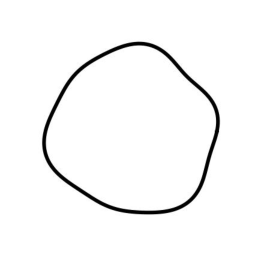
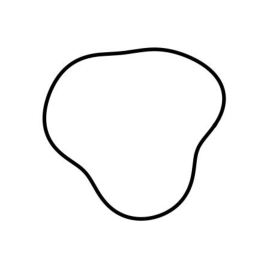
For $\lambda_{2}$, it is also well known that the minimizer over domains of constant area is the union of two equal disks. We start from two eccentric ellipses with size ratio $R_{1}/R_{2}=1.35$, aspect ratios $a_{1}/b_{1}=1.82$ and $a_{2}/b_{2}=0.55$ and optimize their three shape parameters (relative size, both eccentricities) to minimize $\hat{\lambda}_{2}$. The gradient descent converges to $R_{1}/R_{2}=0.99$, $a_{1}/b_{1}=1.08$, $a_{2}/b_{2}=1.05$, while $\hat{\lambda}_{2}$ decreases from $111.52$ to $74.38$, only $2.35\%$ above the exact theoretical value $2\pi j_{01}^{2}/A=72.67$, please refer to Figure 5. Figure 5 also shows the minimizer found for $\lambda_{6}$ presented by Antunes and Freitas. We start from a near circle and it converges to a rounded triangle. The resulting predicted eigenvalue has a $2.5$ relative error compared to the eigenvalue computed with FreeFem.

In this work, we used generative AI tools to expand our first codes as we explored new ideas. We have not used generative AI tools for any other purposes such as drafting the present paper or proving mathematical claims. We have reviewed all AI assisted work. All AI produced code has been checked by at least two authors and most of it has been manually rewritten. We take responsibility for the final content of this work, including text, claims or artifacts produced with the aid of generative AI.

For reproducibility purposes, all random parameters and shapes have been generated with a fixed seed and every experiment can be reproduced.

The codes are available on a github repository https://github.com/devillerochealexis/Neural-networks-for-spectral-optimization.

The weights of the trained torsion function model are available at https://doi.org/10.5281/zenodo.22943009.

We also designed a web app to bundle the Fourier based model, it is available at https://devillerochealexis.github.io/Neural-networks-for-spectral-optimization/

References

- [1] (2012) Numerical optimization of low eigenvalues of the Dirichlet and Neumann laplacians. J. Optim. Theory Appl. 154 (1), pp. 235–257. External Links: Document Cited by: §3.2.
- [2] (2025) Volume-preserving geometric shape optimization of the dirichlet energy using variational neural networks. Neural Networks 184, pp. 106957. Cited by: §2.
- [3] (2024) -PINNs: physics-informed neural networks on complex geometries. Engineering Applications of Artificial Intelligence 127, pp. 107324. Cited by: §2.
- [4] (2025) The landscape function on . Annales de la Faculté des sciences de Toulouse : Mathématiques Ser. 6, 34 (2), pp. 315–337 (en). External Links: Document, Link Cited by: §1.1.
- [5] (2012) New development in freefem++. Journal of numerical mathematics 20 (3-4), pp. 1–14. Cited by: §3.1.
- [6] (2025) Neural sdf for shadow-aware unsupervised structured light. In 2025 IEEE/CVF Winter Conference on Applications of Computer Vision (WACV), pp. 287–296. Cited by: §1.
- [7] (2021) NSFnets (navier-stokes flow nets): physics-informed neural networks for the incompressible navier-stokes equations. Journal of Computational Physics 426, pp. 109951. Cited by: §1.
- [8] (2019) Variational physics-informed neural networks for solving partial differential equations. arXiv preprint arXiv:1912.00873. Cited by: §1, §4.1.
- [9] (2000) Shape descriptors for non-rigid shapes with a single closed contour. In Proceedings IEEE Conference on Computer Vision and Pattern Recognition. CVPR 2000 (Cat. No.PR00662), Vol. 1, pp. 424–429 vol.1. External Links: Document Cited by: §4.2.
- [10] (2026) Finite element eigenfunction network (feenet): a hybrid framework for solving pdes on complex geometries. arXiv preprint arXiv:2602.00870. Cited by: §2.
- [11] (2020) Fourier neural operator for parametric partial differential equations. arXiv preprint arXiv:2010.08895. Cited by: §1.
- [12] (2021) Learning nonlinear operators via deeponet based on the universal approximation theorem of operators. Nature machine intelligence 3 (3), pp. 218–229. Cited by: §1.
- [13] (2021) DeepXDE: a deep learning library for solving differential equations. SIAM review 63 (1), pp. 208–228. Cited by: §1.
- [14] (2019) Deepsdf: learning continuous signed distance functions for shape representation. In Proceedings of the IEEE/CVF conference on computer vision and pattern recognition, pp. 165–174. Cited by: §2.
- [15] (2025) Solving engineering eigenvalue problems with neural networks using the rayleigh quotient. arXiv preprint arXiv:2506.04375. Cited by: §2.
- [16] (2025) Neural geometry processing via spherical neural surfaces. In Computer Graphics Forum, Vol. 44, pp. e70021. Cited by: §2.