MPP-2026-184
Control Problem of de Sitter Vacua with T-brane Uplift
Abstract
T-branes have been argued to provide a consistent uplift to de Sitter vacua in the context of the LARGE-volume scenario of type IIB string theory. We point out that this construction suffers from a serious control problem: the string-frame volume is bounded from above by a number that depends only on the topology of the Calabi-Yau orientifold and is often or smaller. This observation immediately rules out controlled de Sitter vacua in many models with if the non-perturbative superpotential is generated by D3-brane instantons. We give evidence that similar conclusions apply for and show this explicitly for two models with . Our volume bound is seemingly less severe in models where the non-perturbative superpotential is generated by gaugino condensation. However, we study such models and find that, although de Sitter solutions with large volumes are naively possible there, they suffer from uncontrolled warping corrections whose volume suppression is cancelled by other factors, in particular large charges. We also observe that the models with the smallest warping corrections within our set have very small tadpoles and at the same time require a fine-tuned string coupling and flux superpotential, which may indicate an additional problem with the axio-dilaton/complex-structure-moduli stabilization. Finally, we point out an independent challenge related to the stabilization of the brane moduli. Our various results lead us to conclude that it is unlikely that the scenario of T-brane uplifting can be realized in string theory in a self-consistent manner.
1 Introduction
The nature of dark energy is one of the major puzzles of contemporary physics. In the simplest cosmological models, dark energy is a positive cosmological constant, implying that the vacuum state is a de Sitter (dS) spacetime. On the other hand, recent measurements suggest that dark energy may instead vary over time [1, 2]. An intriguing possibility is that such a behavior is a consequence of some yet to be understood principle of quantum gravity. In particular, a concrete research question one may ask is whether string theory forbids dS vacua for some reason and thus predicts that dark energy is dynamical.
Naively, the answer to this question is no since a variety of scenarios for dS vacua have been proposed in string theory (see [3] for a recent review). One of the most popular scenarios is the LARGE-volume scenario (LVS) [4, 5]. Its central claim is that compactifying type IIB string theory on certain types of Calabi-Yau orientifolds yields vacuum solutions (either AdS or dS) in which the volume is stabilized at an exponentially large value so that an excellent control over and warping corrections (which are suppressed by powers of the volume) is achieved. However, while this claim is plausible in the AdS case, it was shown in [6] (and further substantiated in [7, 8, 9, 10, 11, 12]) that it is not true for dS vacua, at least when they are obtained using an anti-brane uplift. Indeed, one then observes that not all types of corrections can be made small at the same time but attempting to control one of them leads to another one blowing up and vice versa. This suggests that LVS dS vacua with anti-brane uplift cannot be constructed self-consistently.
Similar control problems have also been observed in a variety of other dS scenarios in the last few years. For example, the classical-dS scenario [13, 14] was shown to have control problems in [15, 16, 17]11 1 An interesting model circumventing the assumptions of the no-go of [15] was proposed in [18] but is expected to suffer from uncontrolled O5-plane backreaction, as pointed out in (17, footnote 1)., the KKLT scenario with anti-brane uplift [19] was shown to have control problems in [20, 21, 22]22 2 One can construct explicit KKLT dS vacua [23] which avoid the backreaction issues pointed out in [20, 21], but at the cost of a small 3-cycle with a volume of order unity and thus uncontrolled curvature corrections to the anti-brane uplift. See also [24] for a study of a 3d analogue of KKLT with similar control issues., the supercritical dS scenario [25, 26] was shown to have control problems in [27], and for models with a Casimir-energy uplift such problems were shown in [28] (see, however, [29, 30]). Recently, control issues were also observed in the KKLT scenario with -term uplift [31].
In view of these various results, it is natural to suspect that it is a general property of string theory that dS vacua are not possible, at least in the weakly curved and weakly coupled regimes which are computationally accessible. This suspicion also resonates with several swampland conjectures against dS, see, e.g., [32, 33, 34, 35, 36, 37, 38] (see also [39, 40] for a different line of reasoning against dS). However, since these conjectures were mainly motivated by very simple examples, it is a priori unclear under which assumptions they are true and, in particular, why something should be expected to go wrong with more sophisticated constructions like KKLT or the LVS. On the other hand, that something goes wrong is precisely what is suggested by the growing evidence for control problems mentioned above. It is therefore important to understand whether there is a general lesson behind these observations or whether counter-examples exist.
In this paper, we will investigate the claim of LVS dS vacua with a T-brane uplift. For this type of uplift, no issues have been reported so far, which is why it is often presented as a counter-example against seemingly too pessimistic views on dS in string theory. T-branes are non-commutative brane configurations introduced in [41, 42]. They were argued in [43] to provide a consistent dS uplift in the context of the LVS. See also, e.g., [44, 45] for other works using this uplift mechanism.
The main observation of this paper is that the T-brane uplift has a very similar control problem as the anti-brane uplift. In particular, we will show that the string-frame volume in a T-brane-uplifted dS vacuum satisfies an upper bound which only depends on the topological data of the Calabi-Yau orientifold. This bound is highly constraining and yields in many models in which the non-perturbative superpotential is generated by D3-brane instantons. This means that and warping corrections are not suppressed by powers of the volume in such models and therefore not under control.
There are also types of models in which our bound is less severe so that can be stabilized at values significantly larger than unity. In particular, this can happen when the non-perturbative superpotential is due to gaugino condensation with a large-rank gauge group. To assess the viability of such models, we perform a detailed study of 28 different Calabi-Yau orientifolds with . We then scan through all consistent T-brane configurations in these orientifolds, leading to different T-brane models with naive dS vacua. We find that, in spite of the large volumes, warping corrections are not under control in any of these models. This is reminiscent of the LVS with anti-brane uplift, where the impossibility to control warping corrections (simultaneously with other requirements) is also the main issue [6, 7, 8, 9, 10, 11, 12]. In the T-brane case, we argue that the warping corrections are controlled by the parameter (see the main text for definitions) up to an unknown numerical coefficient which we argue to generically be . We then show that cannot be made small within our set of models since the naive suppression due to the inverse volume scaling is always cancelled by some of the other factors, in particular the tadpole . The smallest possible values for we find in our scan are . Hence, the usual LVS claim of a suppression of unknown corrections by an exponentially small control parameter is false in these models.
We also discuss models with and argue that we expect similar control problems there. While we do not perform an exhaustive scan of such models, we confirm our expectation by showing that in two explicit dS models with constructed previously in [44, 45].
We stress that our finding of a large control parameter does not rigorously rule out the possibility of numerically small warping corrections since there might be models in which the unknown numerical prefactors multiplying the corrections are smaller than generically expected. However, since computing all possible corrections explicitly is usually not feasible, moduli-stabilization scenarios in string theory are traditionally based on the assumption of a large-volume and small-coupling regime since then all potentially dangerous corrections are suppressed by powers of these parameters and the exact numerical prefactors are unimportant.33 3 Since the IIB flux landscape is finite for Calabi-Yau orientifolds [46, 47, 48, 49, 50], it is impossible to take limits in which the inverse volume and the string coupling go to zero and the corrections become arbitrarily well controlled. Therefore, the best one can hope for are very small but still finite control parameters. This is different from Calabi-Yau flux vacua in type IIA, where there is evidence that limits of arbitrarily good control are possible, at least in AdS [51, 52]. On the other hand, a construction which purely relies on the hope that something we cannot compute might be very small is much weaker than a construction in which one can plausibly tune a control parameter small. As mentioned before, the paradigm of the LVS is that an exponentially small control parameter is provided by the inverse of the volume, but we show in this paper that this rationale fails for the T-brane uplift. This behavior is reminiscent of anti-brane-uplifted dS vacua in the LVS (and in KKLT) where it was also found that not all corrections can be simultaneously suppressed by small control parameters.
Aside from the warping corrections, we also study the tadpole generated by the O3-planes and curved O7-planes/D7-branes in our set of models. The size of is important since, through the tadpole condition, it determines how many fluxes can be turned on in order to stabilize the moduli and adjust the parameters , (which have to be fine-tuned to get a dS vacuum). An interesting correlation we find in this context is that smaller warping corrections (i.e., smaller ) correlate with a smaller . This is opposite to the anti-brane uplift, where smaller corrections correlate with larger [7, 8]. In the T-brane case, we find that, in models for which is near its lower bound, the (upstairs) tadpole is .44 4 By “upstairs”, we mean that the tadpole is measured on the Calabi-Yau covering space. The “downstairs” tadpole, i.e., the one on the orientifolded space, is . We find it doubtful that such a small tadpole suffices to stabilize all complex-structure moduli and at the same time perform the required fine-tuning in the -plane. Hence, even if one assumes optimistically that the warping corrections are still borderline under control near , models which have a near this value may still not be consistent simply because the moduli cannot be stabilized at the necessary values. While we do not prove this, our observation of small tadpoles suggests that the true lower bound on is actually significantly larger than 1.
This paper is organized as follows. In Section 2, we provide a detailed review of various aspects of the LVS with T-brane uplift. In Section 3, we state the main problem of the T-brane uplift, namely the upper bound on which must be respected in all dS vacua. In Section 4, we discuss a number of potentially relevant corrections to the LVS potential. In Section 5, we perform a scan of T-brane models in Calabi-Yau orientifolds with . We show that in all of these models and that models in which is near its lower bound have small tadpoles. In Section 6, we explain why we expect that models with will have similar control problems as those with . We further study two explicit examples with which indeed turn out to have very small volumes. In Section 7, we point out an additional challenge for vacua with T-branes, namely that they have unstabilized brane moduli if the assumptions of the scenario in [43] hold. In Section 8, we conclude with a few remarks. In App. A, we verify the correct normalization of the T-brane-uplift term. In App. B, we provide some details regarding the algebraic construction of the various Calabi-Yau orientifolds used in our scan.
2 LVS with T-branes
In this section, we review various topics relevant for the LVS with T-brane uplift. We also spell out a few useful details which to our knowledge have not been explicitly discussed before. See also, e.g., [4, 5, 43, 44, 45, 53] for discussions of the LVS and [42, 54, 55, 43, 44, 45] for discussions of T-branes.
2.1 Kähler-moduli Stabilization
We consider the simplest version of the LVS where type IIB string theory is compactified on an orientifold of a Calabi-Yau three-fold with (see Section 6 for the more general case with ). We take to be of Swiss-cheese type, i.e., there is a basis of divisors , such that
| (2.1) |
where , are the divisor volumes, is the Calabi-Yau volume (all in the Einstein frame) and is the Kähler form.55 5 Here and in the following, we denote by the divisors and also the Poincaré-dual 2-forms on . Furthermore, denotes the pullback onto the divisor . The constants , are defined in terms of the triple-intersection numbers
| (2.2) |
and all other triple intersections of and vanish.
The (complex) bulk moduli are the axio-dilaton, complex-structure moduli and Kähler moduli and , where the ’s are axions which will not be important for our analysis. We ignore D7-brane moduli for the moment but will come back to them in the Sections 2.2–2.5. The axio-dilaton and the complex-structure moduli are assumed to be stabilized supersymmetrically using fluxes as in [56, 19]. The dynamics of the two Kähler moduli approximately decouples at large volumes [57, 58] and is governed by an effective supergravity theory with Kähler potential
| (2.3) |
where should be read as a function of and , and is an irrelevant constant that will be set to zero in the following. We included in the leading correction with
| (2.4) |
Here, the first term is the BBHL term [59], where and is the Euler characteristic of the Calabi-Yau manifold. The second term is an orientifold correction derived in [60] which arises in the presence of an O7-plane wrapped on a divisor .
The superpotential is assumed in the LVS to be of the form
| (2.5) |
where , and are constants. The term comes from stabilizing the axio-dilaton and the complex-structure moduli with fluxes [61, 56], while the exponential term is generated by a non-perturbative effect on (see Section 2.6).
From (2.3) and (2.5), we can compute the -term scalar potential with the result
| (2.6) |
Here we already integrated out the two axions , so that the potential only depends on the two real moduli and . We also added by hand an uplift term with (so far) arbitrary coefficient and volume scaling. We will discuss and justify this term in more detail in Section 2.5.
To determine the conditions for dS minima of , we will follow the approach used in [53, 6] for the case of an anti-brane uplift, which we slightly generalize here to arbitrary uplift terms. We first solve the equations of motion for and , which yields
| (2.7) | ||||
| (2.8) |
Here we expanded in to find the solution for and introduced the uplift parameter
| (2.9) |
Substituting the solution into (2.6), we obtain the vacuum energy
| (2.10) |
up to subleading terms in . The (canonically normalized) eigenvalues of the mass matrix in the moduli space are
| (2.11) | ||||
| (2.12) |
up to subleading terms in and . For meta-stable dS vacua, thus has to lie in the range
| (2.13) |
We therefore need an uplift term with , i.e., one that scales less than cubically with the inverse volume in (2.6). The anti-brane uplift satisfies this with [53, 6], whereas the T-brane uplift has , as we will review in Section 2.5.
A common lore is that the LVS construction guarantees exponentially large volumes and therefore an excellent control over and warping corrections (since they are suppressed by powers of the volume). Indeed, according to (2.7), so that it seems that huge volumes are possible as long as we can ensure moderately large . However, this is actually only true for AdS vacua. In dS, the volume is constrained in addition by (2.9) (since , ) and therefore not exponentially large unless we are able to tune the uplift coefficient exponentially small. We will see below that this does not work for the T-brane uplift. In particular, the string-frame volume which controls the and warping corrections will turn out to be tightly constrained by (2.9), to the effect that corrections are not well controlled at all in dS.
2.2 D7-brane Worldvolume Theory
To generate a T-brane uplift as in [43, 44, 45], we assume a compactification in which a stack of D7-branes is wrapped on a divisor with a non-vanishing part along , i.e.,
| (2.14) |
The divisor should furthermore be effective so that the D7-branes are supersymmetric (before turning on worldvolume fluxes) [62, 63, 64, 65]. For Calabi-Yau manifolds obtained as hypersurfaces of an ambient toric variety , effective divisors descend from positive integral linear combinations of the irreducible divisors of . This implies , in the models we will study in this paper.66 6 In the models we will consider, the irreducible divisors are combinations of positive integer multiples of and integer multiples of , and therefore the effective divisors are as well (cf. App. B). In principle, Calabi-Yau manifolds can have additional effective divisors which are not effective on the ambient space and need not be positive linear combinations of the irreducible ones (see, e.g., [66, 23] for discussions). It is not known how to compute them in general so that we will not consider them. Since is an orientifold-even divisor, the gauge group is either SO (if the divisor is pointwise invariant, i.e., the branes lie on top of an O7-plane) or USp (if the divisor is invariant but not pointwise, i.e., the branes do not lie on top of an O7-plane) [67]. Note that in our convention counts the “upstairs” brane number in the stack, i.e., including image branes.
The local physics of the D7-branes is described by a twisted 8d super-Yang-Mills theory with an internal -form (i.e., its legs are along ) and a 1-form gauge field [68]. In a 4d vacuum, the internal background fields satisfy the -term and -term equations
| (2.15) |
where denotes the pullback of harmonic 2-forms on onto the brane worldvolume . Furthermore, is the gauge-invariant field strength77 7 We work in units where .
| (2.16) |
where is the usual Yang-Mills field strength and is the NSNS 2-form. We use here the conventions of [69] where (2.15) was derived from the non-Abelian DBI action.
Note that (2.15) is valid for small , large and small brane fields since the equations ignore backreaction effects (warping, varying dilaton, etc.) and corrections. They furthermore do not take into account the effect of bulk fluxes. The latter couple to in the D7-brane action [70, 71, 69] and thus yield a correction to the equations of motion that will be responsible for the T-brane uplift [43]. We will discuss this and other corrections in more detail later but assume for the moment that (2.15) holds in order to study the leading-order dynamics of the brane fields.
Before we do so, let us also make a few comments on the orientifold projection. Without orientifolding, , and are valued in the adjoint of U. We can thus expand
| (2.17) |
where the ’s are (2,0)-forms, the ’s are real 1-forms, the ’s are real 2-forms and the ’s with are the U generators, which in our convention are Hermitian. The orientifolding imposes constraints on these fields so that some of their components are projected out [72, 73] (see also, e.g., [64, 74, 67, 75] for discussions of the D7-brane case). One finds
| (2.18) |
where is the orientifold involution and is an matrix which, up to a basis change, equals either (for a D7 stack on top of an O7-plane)88 8 A common choice in the literature is to take instead , which is related to our choice by , , , with . or (for a D7 stack on an orientifold-even but not pointwise invariant divisor).99 9 Determining the correct sign in the constraint for is somewhat subtle. To verify it, consider a Calabi-Yau manifold with local complex coordinates , , and an orientifold-invariant D7 stack located at . We then have in terms of the holomorphic -form and the adjoint worldvolume scalar describing the normal deformations of the branes [64, 69]. Since for O3/O7 orientifolds [76, 77], we further have , where the upper sign is for a stack on top of an O7-plane (i.e., for an involution ) and the lower sign is for a transversally intersecting stack. Using this, (2.18) is equivalent to . Taking as a simple example two D7-branes on top of an O7-plane and assuming a constant scalar vev along the worldvolume, we obtain for some constant . Hence, the position of a brane moved off the O7-plane is constrained to be minus the position of its image, consistently with what one would expect. For a transversally intersecting stack, we instead get so that the two branes can only move as a pair, which is consistent with observations in [78, 79, 74]. Note that the constraint on only holds up to (large) gauge transformations shifting and , which we will come back to in Section 2.4.
The projection with symmetric is sometimes called SO projection since, for vanishing vev and background flux, it yields a massless 4d gauge field in the adjoint of SO (as follows from (2.18) using that on a pointwise-invariant divisor). When a vev or flux is turned on, some of the 4d gauge bosons become massive and the gauge group is broken to a subgroup of SO. The projection with anti-symmetric is called Sp projection since, for vanishing and flux, it yields a massless 4d gauge field valued in the adjoint of USp (note that the zero mode of does not depend on the internal coordinates and thus satisfies ). To work out how the projection constrains and the internal components of , , we have to take into account that they split into orientifold-even and odd forms (e.g., with ), which are in different representations. In particular, for the Sp projection, (2.18) implies that orientifold-even forms are valued in the adjoint of USp, while orientifold-odd forms are valued in the two-index anti-symmetric representation. For the SO projection, we only have to consider orientifold-even forms since there are no odd ones on a pointwise-invariant divisor. The former are valued in the adjoint of SO. See, e.g., [80] for a review.
As an example, consider the case . The gauge group before orientifolding is then U so that we can write
| (2.19) |
and analogously for . After the orientifold projection, the surviving components are
| (2.20) | ||||||||
| (2.21) |
where the subscripts indicate orientifold-even/odd 2-forms.
For general , (2.18) implies that, up to basis changes, and take the form
| (2.22) | ||||||||
| (2.23) |
in terms of matrices (whose entries are 2-forms), where are Hermitian, , are anti-symmetric, , are symmetric, are unconstrained and the subscripts again stand for orientifold-even/odd. We thus see that, on general D7 stacks, both even and odd forms arise in the non-Abelian worldvolume fields. The T-brane vacua we will study in this paper have diagonal fluxes with and off-diagonal vevs with . Hence, the fluxes we will consider are orientifold-even, while can in general acquire orientifold-even or odd vevs in our setup.
2.3 T-branes
We now want to construct a T-brane solution to the -term and -term equations (2.15). T-branes are solutions in which acquires a vev in the upper-right triangle above the diagonal (hence the “T”) such that [42]. This can be interpreted as a bound state of the D7-branes in the stack. To obtain such a configuration, we turn on a worldvolume flux valued in the Cartan subalgebra of the gauge algebra. For convenience, we choose a basis of generators such that the Cartan generators are diagonal (and traceless) matrices.1010 10 For SO, this would not be the case in the standard basis where the generators are anti-symmetric matrices. However, in the basis we chose in Section 2.2, we can take diagonal fluxes for both SO and USp, cf. (2.22), (2.23). We further take the flux on the branes and their orientifold images to be the same up to a minus sign as in [43, 44, 45]. Our ansatz is thus
| (2.24) |
where is a closed 2-form on . The non-trivial gauge bundle in this case is a direct sum of line bundles with curvatures . The first equation in (2.15) implies that in cohomology [63, 68] and, according to (2.22), (2.23), must furthermore be orientifold-even. We also require to not be primitive,
| (2.25) |
since otherwise the -term equation (the last one in (2.15)) yields and no T-brane is possible.
In order to solve (2.15) in the presence of the flux, we can locally make the ansatz
| (2.26) |
for some real , where , are complex coordinates on .1111 11 Here we assume for simplicity so that . For , we instead have . Hence, acquires an extra term compared to (2.26). This does not affect the solution for since it cancels out in (2.15) (in particular, in ). We further make the ansatz (valid again in a local patch of )
| (2.27) |
where is a closed -form and is an matrix satisfying . Globally, is a cohomology class in (see (69, Secs. 5 & 6) for more details). According to (2.22), (2.23), it depends on the gauge group and the choice of whether is orientifold-even or odd: In the USp case, has to be orientifold-odd for anti-symmetric and orientifold-even for symmetric . In the SO case, only orientifold-even and anti-symmetric is allowed.1212 12 Note that this implies that T-branes can only exist for in the SO case, consistent with the fact that SO is an Abelian group and thus cannot yield solutions with . In the USp case, T-branes are possible for any even , the simplest example being with gauge group USp SU.
Substituting (2.26) and (2.27) into (2.15), we see that the two -term equations are automatically solved and the -term equation reduces to a differential equation determining :
| (2.28) |
We refer to [42, 54] for more details on how to solve this equation. For the purpose of this paper, it will be sufficient to know that we consider T-brane backgrounds with a diagonal flux of the form (2.24) and an off-diagonal vev of the form (2.27).
2.4 Constraints on the Worldvolume Flux
Let us now discuss in more detail which fluxes can be turned on. In general, contains elements which are pulled back from harmonic forms on the ambient Calabi-Yau (i.e., forms in ) and elements which cannot be obtained from such pullbacks. See, e.g., [81, 82, 67, 83] for discussions. Pullback -forms are necessarily orientifold-even in our setup (recall that we assume ), while -forms that are not pullbacks can have even and odd pieces in general. One can furthermore choose a basis of -forms such that the pullback basis forms are orthogonal to (i.e., wedge to zero with) the non-pullback basis forms. We will call any -form that is a linear combination of the latter type of basis elements “variable”, following the terminology of [83]. The cohomology group thus splits into two subgroups: . Since a T-brane requires , it is clear that must contain a pullback piece (consistently with the fact that, as explained previously, is orientifold-even). We can thus write
| (2.29) |
up to exact terms1313 13 As explained in [54], is not harmonic in a T-brane background., where , are some (yet to be determined) flux numbers and denotes possible variable fluxes that wedge to zero with the two pullback terms. Note that, in the case , there is no component since the pullback of the form onto the divisor then vanishes.
We now discuss the quantization conditions for , . The worldvolume flux is quantized as [84, 85, 67]
| (2.30) |
where we used that on a Calabi-Yau manifold and the notation on the right-hand side means that all elements of the matrix on the left-hand side are in .1414 14 Note that this formula holds for Abelian flux and only in a basis where the Cartan generators are diagonal, as the matrix is not basis-invariant. More specifically, they are in since , and are all -forms. Using furthermore (2.24) in (2.30) yields
| (2.31) |
Determining the elements of is somewhat subtle. One may think that they are simply given by for some and some variable form . However, this is in general not correct and instead also fractional values of , can occur. This can happen for three reasons:
- •
- •
Furthermore, the pullback forms in need in principle not be inherited from but may also come from . In the latter case, has elements with and even when , are an integral basis of . It was argued in [86] that this cannot happen for divisors for which the Lefschetz hyperplane theorem holds. However, this requires to be ample (i.e., to lie in the Kähler cone), which is in general not true for .1515 15 As stated before, one should however impose that is effective.
- •
Even when the above two caveats do not apply – i.e., when all pullback forms in have integral , – it can still happen that the group contains non-pullback forms with and . Such group elements mixing fractional pullback and variable terms were called “glue vectors” in [86]. Their appearance means that – unlike – does typically not split into two subgroups: . Instead, the pullback forms and the variable forms only generate a sublattice of the full lattice of all integral group elements. The missing elements form a finite subgroup of which is generated precisely by the glue vectors [86].1616 16 As an illustrative example, consider the case . Assuming that consists of integer combinations of and , the pullback forms inherited by are and integer multiples thereof (since vanishes). Now, if were the generator of an integral subgroup , there would have to be a basis 2-cycle over which this form integrates to 1, and the Poincaré dual of this 2-cycle would have to equal for some . However, , which cannot equal 1 whenever . Hence, it is clear in this case that does not generate an integral subgroup and therefore .
The upshot of the discussion is that , need not be integers unless , are an integral basis of , is ample, and variable forms are turned off. Due to these caveats, it is in general a highly non-trivial task to identify the elements of and, consequently, the correct quantization of the flux numbers , .
Luckily, the first caveat will not play a role in this paper since, in all models we will consider, and are an integral basis of (with the exception of one model briefly discussed in Section 6 which will be treated separately). In order to bypass the other two caveats, we will furthermore restrict to elements of pulled back from . This assumption greatly simplifies the analysis and is still general enough to allow us to study a variety of different models. Note that here we follow previous works on T-brane uplifting [43, 44, 45], which made the same assumption.
To summarize, the elements of we consider in (2.31) are of the form with . Using this together with (2.14), we arrive at
| (2.32) |
where we took the upper sign in (2.31).1717 17 One can verify that taking the lower sign eventually leads to the same constraint (2.35).
The last remaining piece to understand is the field. Since is odd under , it naively has to satisfy so that only components in survive the orientifold projection. This would mean that has to vanish in our setup since we have by assumption. However, as discussed, e.g., in [87, 67, 75], there is a discrete shift symmetry , with so that satisfying is sufficient to survive the orientifolding. This admits in particular a half-integrally quantized . Pulling this back onto yields
| (2.33) |
Combining (2.33) and (2.32), we conclude that
| (2.34) |
Since , , , , , are all integral, it follows that we can choose any half-integral , by turning on an appropriate . We will furthermore see in Section 2.6 that the consistency of the LVS requires . Hence, the allowed flux numbers are
| (2.35) |
We stress again that one of the models discussed in Section 6 is an exception to this rule (e.g., is allowed there).
Finally, a further constraint on the flux numbers comes from requiring that the solution to (2.28) is globally well-defined on the compact submanifold wrapped by the T-brane. As shown in [54, 88], this is the case if1818 18 The inequalities (2.36) can be violated in the presence of a localized defect in the D7-brane worldvolume theory [55]. Such a defect can arise, e.g., when a second brane stack intersects the stack on and the bifundamental degrees of freedom at the intersection acquire non-trivial vevs. The resulting solution is then a bound state of both brane stacks. In our case, one could in principle consider bound states of the branes on and those on but it is not clear to us whether such configurations admit the non-perturbative superpotentials required by the LVS. We will therefore not consider them but assume following [43, 44, 45] that there is a T-brane on and an independent second brane stack (or instanton) on that generates . Note that the key problem pointed out in Section 3 gets worse when (2.36) is violated (as this implies larger flux) so that defects are not promising loopholes from that perspective.
| (2.36) |
where we again used that on a Calabi-Yau manifold. This yields
| (2.37) |
where we used (2.14), (2.29), (2.35) and assumed in the Kähler cone as usual in the LVS. We thus find that the flux numbers must satisfy the following bounds:
| (2.38) |
2.5 Uplift
We now explain how the T-brane setup of Section 2.3 leads to an uplift term in the LVS potential (2.6). From the point of view of the 4d effective field theory, the D7 stack on generates a -term potential [69]
| (2.39) |
Here, denotes the harmonic part of (with respect to the gauge-covariant derivative ) rescaled such that . In this normalization, the Kähler potential for is . In general, also depends on Wilson-line moduli which however vanish in the T-brane background and are already set to zero here. For more details, we refer to [69] where the general -term potential of a non-Abelian D7 stack was derived by dimensionally reducing the DBI action (see also [64, 81, 89, 90] for results in the case of a single D7-brane and [70, 68, 91, 92, 54, 43] for related work in the non-Abelian case).
The potential is minimized for
| (2.40) |
where we used (2.14), (2.24), (2.29) and (2.35). Clearly, (2.40) is the 4d version of the -term equation in (2.15). As discussed in Section 2.3, the solution is a T-brane background with . Using this, (2.40) implies
| (2.41) |
As stated before, turning on bulk fluxes generates extra couplings in the D7-brane worldvolume theory and thus modifies the dynamics of the brane fields [70, 71, 69]. From the 4d point of view, this generates an -term potential [69] (see also App. A)
| (2.42) |
This expression is valid if the superpotential is independent of the brane moduli, as assumed in the T-brane-uplifting scenario [43, 44, 45]. We refer to [69] for more general expressions for and for the superpotential of non-Abelian D7-branes (see also [81, 90, 65, 93] and [94, 91] for earlier work on the Abelian/non-Abelian brane superpotential, respectively). Note that both and receive various corrections, in particular and backreaction corrections as well as corrections from integrating out KK modes. We will come back to some of these corrections in Section 4. An extensive discussion of KK corrections to the D7-brane potential is provided in [69].
The minimum of is now obtained as follows. For sufficiently small and large , (2.42) is much smaller than (2.39) so that still satisfies (2.41) in the minimum up to a subleading term. Using (2.41) and in (2.42), we find
| (2.43) |
We thus observe that the T-brane generates a positive term in the scalar potential. Identifying this with the uplift term anticipated in (2.6), we conclude
| (2.44) |
This agrees with the uplift term derived in (43, (2.33)) and with those in (44, (4.22)), (45, (5.29)) up to a factor (upon using the values of , in these setups). Note that the factor is important since, as we will see, the maximal volume in a T-brane-uplifted dS minimum scales like . This can be a very small number, e.g., when the T-brane bound state is made out of D7-branes. Let us emphasize again that (2.44) is consistent with the dimensional reduction performed in [69], where we derived the full non-Abelian -term and -term potential of the D7-branes.
As we mentioned, our approximation of minimizing and then substituting the result into is only valid when is much steeper than . If this is not the case, we should instead minimize the full potential in a single step. To this end, one can make the ansatz , for some complex 4d scalar field . Substituting this into (2.39), (2.42), we get
| (2.45) |
where we used that , in the LVS and neglected terms that would only give subleading corrections to the solution compared to the effect of the term. One verifies that, if
| (2.46) |
holds, the equation of motion has two solutions: the trivial solution and the T-brane solution , where is an arbitrary phase and
| (2.47) |
If the second term in the square root is small, we recover the approximate solution obtained by minimizing the -term potential. On the other hand, if the susy-breaking by becomes too large, i.e., if (2.46) is violated, the T-brane solution vanishes and the only solution is . In that case, we also expect higher--term/KK corrections to become important so that we can no longer trust the potential anyway, see Section 4.2.
Let us also check the stability of the T-brane by substituting into the potential, where is a real fluctuation. Expanding up to the second order in , we get1919 19 We have set in this expression for simplicity. For , a further term with the same volume scaling as the correction appears in the mass term.
| (2.48) |
If (2.46) is satisfied, the term has a positive coefficient and therefore the T-brane is meta-stable against a decay to other brane configurations, at least along this particular direction in the field space. As stated before, the phase is not stabilized. We will make further comments on the brane-moduli space of T-brane vacua in Section 7.
2.6 Non-perturbative Effect
A crucial requirement for the LVS is that a non-perturbative term as in (2.5) is present in the superpotential. Such a term can either be generated by D3-brane instantons (E3-branes) or gaugino condensation on D7-branes wrapped on the divisor [95, 19]. In order for this to happen, a number of conditions must be satisfied, which we review in this subsection. See [80, 96] for more detailed reviews of instantons and [97, 98] for discussions of some aspects of gaugino condensation. Non-perturbative effects in the LVS/T-brane context are discussed in [44, 45].
Let us first recall the involved gauge groups. Since is orientifold-even, the (continuous) gauge group of a stack of D7-branes on is either SO (if the branes wrap a pointwise-invariant divisor and thus lie on top of an O7-plane) or USp (if the branes do not lie on top of an O7-plane). For the instantons, it is the other way round: a stack of E3-branes on has the gauge group USp if the divisor is pointwise-invariant and SO otherwise [80, 67, 96]. Since symplectic groups have , a single E3-brane only exists on a not-pointwise-invariant divisor and has gauge group O.
In order to generate a non-perturbative superpotential, E3-branes need to have exactly two fermionic zero modes. Let us ignore intersections with other branes for the moment and postpone their discussion until the end of this subsection. A sufficient (but not necessary) condition for E3-branes to have exactly two fermionic zero modes is then that the gauge group is O and is a rigid divisor, i.e., [95] (see [80, 96] for reviews). The case of D7-branes with gaugino condensation is very similar: A non-perturbative superpotential is then generated if the worldvolume theory is pure super-Yang-Mills theory at low energies, i.e., there are no massless matter fields valued in the adjoint or (anti-)symmetric representations of the gauge group, which is again ensured by wrapping a rigid divisor [97, 98].
Rigidity of a divisor implies that the arithmetic genus satisfies . On a Calabi-Yau three-fold , this can be checked using the formula
| (2.49) |
where is the second Chern class of . The models we consider in this paper all satisfy . More generally, also E3-branes or D7-branes on non-rigid divisors can contribute to due to the effect of fluxes. Indeed, worldvolume or bulk fluxes can “rigidify” a non-rigid divisor by lifting unwanted fermionic zero modes or massless matter fields that would prevent the generation of a superpotential [99, 100, 101, 102]. However, this is often difficult to check in practice so that rigid divisors are usually the easiest way to guarantee a non-perturbative superpotential.
Let us also briefly discuss higher-rank instantons, i.e., stacks of E3-branes with . Without fluxes, such instantons have at least four fermionic zero modes and thus do not contribute to , even when the divisor is rigid [80, 96].2020 20 Similarly, instantons wrapping divisors in the class for do not contribute to without fluxes since implies for . However, fluxes can again lift some of these zero modes in which case instantons with can appear in [103].
Depending on which of the discussed effects generates , one finds
| (2.50) |
The last two expressions follow from the general formula , where is the dual Coxeter number of the gauge group [97, 98].2121 21 There are conflicting statements in the literature about which can host a non-perturbative effect (see, e.g., [104] for models with USp gauge groups and [53] for a comment that only SO is allowed). We will not go into the intricacies of this discussion and, to be as general as possible, study models with USp and SO gauge groups of various ranks.
Aside from too many zero modes, another possible obstruction to generating a is the quantization of the worldvolume flux. As discussed in Section 2.2, the flux is constrained by the orientifold projection. This applies to instantons and spacetime-filling branes alike (with the mentioned caveat that the gauge groups of pointwise-invariant and not-pointwise-invariant instantons are interchanged compared to the D7 case). For an instanton with O gauge group, the projection is such that only orientifold-odd flux is allowed [83]. Since we assume in this paper, this means that the flux on the instanton has to vanish (up to variable terms, which we ignore for the moment). If comes from D7-branes instead of an E3-brane, the orientifold projection would in principle allow orientifold-even flux (just like it does for the D7-branes on , cf. (2.22), (2.23)). However, this would break the SO or USp gauge group to a subgroup, create chiral matter fields, generate a -term potential and generically recombine the branes, all of which can prevent a contribution to . We will therefore follow the LVS literature [44, 45] and assume vanishing flux on the D7 stack. In summary, we are led to impose2222 22 To avoid confusion, note that refers to the flux of the D7 stack on , while is the flux of the D7 stack on .
| (2.51) |
The flux-quantization condition under this assumption becomes [84]
| (2.52) |
In the LVS context, is typically a non-Spin divisor so that is not an element of .2323 23 For complex manifolds, not having a Spin structure means that is not an element of . We further have since is a divisor on a Calabi-Yau manifold. Hence, (2.52) can only be satisfied if a half-integral with is turned on (modulo integral forms). However, this trick does not always work since there can be situations where one is forced to set . This happens, e.g., if the T-brane wraps a divisor with even , as follows from (2.33)–(2.35). In such a case, an E3-brane or a D7 stack satisfying (2.51) cannot generate a because their existence is forbidden by the flux-quantization condition. Hence,
| (2.53) |
There are however loopholes to this conclusion: instantons with variable flux [105] or higher-rank instantons with non-Abelian flux [103] can be consistent with the orientifold projection and flux quantization in spite of . Such effects can ensure that a is generated also in models with even . See, e.g., [45] for an LVS model using a rank-2 instanton.
A final constraint we need to discuss comes from zero modes or massless matter fields localized at the intersections between different branes or brane stacks (in our case, the branes or instantons hosting the non-perturbative effect on and the branes wrapped on ). As mentioned in the beginning, such modes have to be absent in order that a is generated, and this is not guaranteed by imposing rigidity of . An easy-to-check necessary condition is in particular that the chiral index – i.e., the number of chiral minus anti-chiral zero modes – vanishes at the intersection. The formula for two branes on divisors , with gauge bundles , is [106, 67, 68, 96]
| (2.54) |
Applying this to the intersection of a D7-brane on (or its image) and an E3-brane on , we obtain
| (2.55) |
where we used (2.29) and (2.51). Hence, in order to generate a , we have to set the component of to zero in (2.29),
| (2.56) |
One can verify that the same condition must hold if the instanton carries a variable flux and also for instantons of higher rank.2424 24 Variable flux satisfies by definition (cf. our discussion above (2.29)) and thus does not affect (2.55) [67]. The generalization of (2.54) to brane stacks with higher-rank gauge bundles , is [96]. Applied to the case of D7-branes on and a rank- instanton on , this yields , where the second term vanishes since the orientifold projection imposes that is orientifold-odd and thus variable, i.e., . One thus gets the condition as in the rank-1 case. Note, however, that this is only sensitive to the overall chiral intersections for the whole E3 stack. Detecting chiral intersections of individual E3-branes and D7-branes or of pairs of E3-branes would require a more refined computation. An analogous argument can also be made in the case where the non-perturbative effect comes from D7-branes with gaugino condensation instead of instantons.
We finally note that there can be further obstructions to a non-perturbative superpotential beyond those discussed in this subsection (see, e.g., (45, footnote 21)). We will not study such subtleties in detail. The point of this paper is that LVS models with T-branes do not yield a controlled dS uplift, and this conclusion does not change if some of these models happen to have additional problems.
2.7 Tadpole Cancelation
Let us also collect a few useful formulae related to tadpole cancelation. Our T-brane setup involves a stack of D7-branes on the divisor and optionally another stack of D7-branes on the divisor (if the non-perturbative effect is due to gaugino condensation). In the models we will consider, the orientifold involution further yields an O7-plane wrapped on
| (2.57) |
and, in some cases, additional O3-planes counted by the number of isolated fixed points of the orientifold involution. To cancel the D7 charges of the D7-branes and the O7-plane, we have to impose the tadpole condition
| (2.58) |
Here, and denote the number of branes in the upstairs convention, i.e., on the covering space of the orientifold where image branes are also counted.
The D7-branes, O7-plane and O3-planes further carry a D3 charge
| (2.59) |
again in the upstairs convention. This charge has to cancel with the D3 charges carried by bulk fluxes and D3-branes:
| (2.60) |
where is the number of D3-branes (counting also orientifold images). The bulk fluxes are imaginary self-dual, i.e., , so that [56]. Together with , this implies that is negative.
A useful formula for the Euler number of a divisor is
| (2.61) |
where is the second Chern class of . Writing 2525 25 Note that terms vanish since the only non-vanishing triple-intersections are given by (2.2)., (2.59) becomes
| (2.62) |
For later convenience, we also state a formula for the number of complex-structure moduli . To this end, we combine the standard formula for the Euler number and the Lefschetz fixed-point theorem (see, e.g., [107]), which in our case states . This yields
| (2.63) |
3 The Volume Bound
In this section, we describe the main problem of the T-brane uplift. Our claim is that the string-frame volume is bounded in any dS vacuum such that the possibilities to control corrections to the LVS approximation are severely limited. Indeed, using (2.44), (2.4) and in (2.9) yields
| (3.1) |
Note in particular that this does not depend on or . Furthermore, is bounded from below since it is quantized and depends on the number of D7-branes on which, by tadpole cancelation, is tied to the O7-planes. How strongly (3.1) constrains the volume is therefore completely determined by the topological data of the Calabi-Yau manifold and the choice of orientifold involution.
To illustrate the strength of the bound, let us consider manifolds where , are an integral basis of and worldvolume fluxes of the pull-back type, as explained in Section 2.4. We can then further simplify (3.1) by using . This follows from tadpole cancelation on (which, according to (2.58), implies ) together with flux quantization (which, according to (2.35), implies ). Since is an integral combination of and , we further have . The bound thus becomes
| (3.2) |
An immediate consequence of this is that large-volume dS vacua are ruled out in these models if the non-perturbative effect is due to instantons (i.e., ). To see this, note that is typically of the order or smaller and that, as will be detailed in Section 5, Swiss-cheese Calabi-Yau manifolds with satisfy . We thus find
| (3.3) |
and therefore dS vacua with large volumes are excluded in these models! Instead, the maximal size of the Calabi-Yau manifold is of the order of the string length. We therefore expect an infinite number of (and warping) corrections to become relevant and the LVS potential to no longer be reliable. We stress that it is the string-frame volume, not the Einstein-frame volume , which controls the expansion. Having a large Einstein-frame volume is in principle consistent with our bound for sufficiently small but this is irrelevant for the degree of control. An alternative perspective to this problem is to consider the KK scale, which is of the order in string units and thus approximately equals the string scale. We are thus at the boundary of the regime where the description in terms of a 10d supergravity theory (and the 4d effective theory derived from compactifying it on a Calabi-Yau) is valid, suggesting that instead a fully non-perturbative string-theory calculation would be required.
Let us also note that, even ignoring string corrections and focussing just on supergravity, the derivation of the standard LVS potential (2.6) assumes in various steps, e.g., for the crucial decoupling between the axio-dilaton and the Kähler moduli [57, 58]. The former is assumed to be frozen to a constant in the LVS, although its stabilized vev is in reality a function of , due to the mixing term in the Kähler potential. The approximation of neglecting this dependence is only valid if , since then the equation is approximately independent of the Kähler moduli. Hence, also from this perspective, it is clear that solutions with small are not in a trustworthy regime.
Finally, there are also models for which (3.2) is less constraining than in the instanton case and in fact compatible with relatively large volumes (of the order ) so that no immediate problem seems to arise, neither regarding corrections nor the decoupling approximation. It is obvious from (3.2) that the weakest constraints on the volume are obtained for large Euler numbers, small intersection numbers and a non-perturbative effect from gaugino condensation with a large-rank gauge group (since then is much smaller than in the instanton case). However, we will see that even in these naively favorable models the volume is never large enough that warping corrections are under control. Hence, these models are put into serious doubt by our volume bound as well. Demonstrating this in detail will be the topic of the following sections.
4 Corrections
In this section, we discuss a few potentially dangerous corrections to the potential (2.6). In general, many different types of corrections can appear in the effective field theory and one has to check that all of them are sufficiently suppressed, see, e.g., [108, 6, 109] for an overview. We will not attempt to provide an exhaustive analysis here but focus on warping/backreaction corrections. Indeed, the impossibility to control such corrections in a T-brane-uplifted dS vacuum will be a key point of this paper.2626 26 As emphasized in [6, 110], another potential threat for the LVS is due to logarithmic redefinitions of the Kähler coordinates, which will however not be discussed in this paper. We will also briefly discuss higher--term corrections and point out that they are automatically controlled once the warping corrections are controlled.
4.1 Backreaction of D3 Charge
On an approximately isotropic space, a codimension-6 object with D3 charge such as an O3-plane is expected to generate backreaction corrections of the order at generic2727 27 Very close to the source, at distances , the backreaction becomes larger and eventually diverges like since, for , the Green’s function is the flat-space one up to subleading corrections. points, where is the string-frame length scale characterizing the space. On spaces with large anisotropies, one instead expects a backreaction of the order , where is the diameter in the string frame [27].2828 28 See also [111] for the case where the anisotropy is due to a large-complex-structure regime. Since can be much larger than , the backreaction in the anisotropic case is parametrically larger than in the isotropic case, the intuitive reason being that the effective codimension is lowered when the manifold is stretched such that it becomes very thin in some directions and very long in others. We can therefore take the isotropic case as a conservative estimate for the expected backreaction.
Aside from D3-branes and O3-planes, also D7-branes and O7-planes carry D3 charges in the presence of fluxes or curvature on their worldvolumes. Instead of sources , we then schematically have sources in the 10d equations of motion. For branes/O-planes wrapping the big divisor, this yields with . The Green’s function grows logarithmically in the distance for and approaches some maximum of the order at some inbetween the branes. Neglecting the logarithmic scaling, the backreaction is thus again of the order just like for the O3-planes. We expect the same for D7/O7s wrapping the small divisor since they should look like an O3-plane at distances much larger than the size of the blow-up cycle (which at large volumes is true at generic points on the Calabi-Yau).
The localized negative D3 charges from the O3-planes, D7-branes and O7-planes generically do not cancel locally with the positive charges provided by the bulk fluxes since the latter spread out over the manifold in the regime of large volumes and weak warping assumed in the LVS.2929 29 In principle, flux densities can be exponentially localized in strongly warped regions of the Calabi-Yau (Klebanov-Strassler throats [112]). One may then try to place O-planes nearby that exactly screen the local charge density of the fluxes [21]. If this can be done for most of the fluxes on the Calabi-Yau, the effectively backreacting D3 charge in the Calabi-Yau bulk would be much smaller than , leading to an essentially unwarped Calabi-Yau bulk “spiked” with lots of strongly warped Klebanov-Strassler throats. We will not try to estimate the 4d warping corrections in this highly ungeneric situation but assume in this paper a generic distribution of a positively charged flux density and negatively charged localized sources, without local cancelations that parametrically affect the strength of the backreaction. We therefore generically expect that the total warping corrections are of the order
| (4.1) |
where we recall that is the D3 tadpole generated by O3-planes, D7-branes and O7-planes. In simple spaces such as 6-tori, one can explicitly check that this parametric behavior is correct [27].

As pointed out in [6], a concrete example of a warping correction to the LVS potential arises for the BBHL term in the Kähler potential (cf. (2.3), (2.4)), where is the Euler class of . The BBHL term can be inferred from a correction to the 4d Einstein-Hilbert term that arises from dimensionally reducing the 10d term of type IIB string theory [59]. In the presence of a non-trivial warp factor , this is corrected as
| (4.2) |
The warping correction thus amounts to replacing in (2.6), where we included an unknown numerical coefficient which we assume to be (see below for a discussion). Hence, we expect that the LVS potential (2.6) receives a warping correction
| (4.3) |
Note that warping corrections are also expected to appear in other places, e.g., in the -term potential and the uplift term, whose derivation also assumes an absence of warping. Here we will consider the effect of the above correction as a proxy to estimate the control over warping corrections, but one should keep in mind that this is certainly not the only warping correction that will appear.
As explained in [21] (see also (17, Section 2.3)), warping corrections have to be small at generic points3030 30 Note that demanding small warping at every point would be too restrictive since the warp factor and other fields typically have singularities in the vicinity of the localized sources where, e.g., the curvature blows up. This is not an inconsistency per se as long as the singular regions are smaller than a string length and the compactification volume is much larger than that. Since supergravity is an EFT valid at energies below the string scale, a breakdown of the supergravity solution at small distances is expected and by itself not concerning. on the Calabi-Yau since otherwise one expects a “singular-bulk problem”, i.e. the warping is so strong that large parts of the naive geometry are eaten up by a classical singularity. Although this singularity is expected to be a supergravity artifact cured in string theory [113], this does not mean that it is harmless. Indeed, as emphasized in [21], the resulting compactification will be strongly curved and stringy and no longer amenable to a supergravity treatment. See Fig. 1 for an illustration. We therefore need to make sure that warping corrections of the above sort are small in candidate flux vacua.
In the LVS, the problem is exacerbated by the fact that the corrections to the vacuum energy and to the eigenvalue of the Hessian (defined in Section 2.1) are by a factor stronger than the corresponding corrections to the off-shell LVS potential [6]. This is due to a specific cancelation effect which was called non-perturbative no-scale structure in [6] since it is related to the exponential dependence of .3131 31 The fact that is by a factor smaller than the individual off-shell terms in was already observed in [114]. The new observations in [6] were that an analogous cancelation also occurs in , that a no-scale structure is responsible for these cancelations and, most importantly, that they have the effect of a parametric enhancement of warping and other corrections to and . A consequence of this is that candidate LVS vacua are already in danger at a parametrically smaller warping than what would cause a singular-bulk problem. Explicitly, we find by adapting the results of [6] to the T-brane uplift that the leading warping corrections to and satisfy
| (4.4) |
Here , denote the leading warping corrections to and , respectively. Note that there is no suppression in these corrections, unlike in (4.3), as predicted by the non-perturbative no-scale structure. Clearly, we have to demand , for control.
A conservative estimate of the corrections is obtained by taking so that both terms in (4.4) are equal in size. Closer to the boundaries of the dS range , either the correction to or the one to would blow up. Assuming further as stated above, we are led to define the following condition for control:
| (4.5) |
In the remainder of this paper, we will take as a proxy to measure how dangerous the warping corrections are in a given model.
Before we move on, a word of caution is in order. As usual for a parametric estimate, we do not know the precise value of for which the unwarped approximation breaks down since we do not know the numerical prefactor in (4.4). As stated before, the plausible assumption of a correction to the Euler number implies and thus motivates (4.5). However, we cannot exclude that is numerically small in certain cases so that demanding (4.5) may be too strict. Our philosophy regarding this loophole is that a dS construction is only under control if all ignored corrections are shown to be negligibly small, either by explicit computation or by identifying a small parameter by which the corrections are suppressed (in this case ). The advantage of the second option is that we can bypass a full computation of the corrections as long as we know their scaling with the parameter and convince ourselves that the parameter can be tuned small.3232 32 As stated in the introduction, it is impossible in type IIB to take control parameters to zero but we can at least try to make them very small. On the other hand, a dS model whose consistency relies purely on the hope of a small without computing it is in our view not under control. Indeed, it is usually not feasible to compute all warping (and other) corrections in full explicitness including numerical factors, and therefore suppressing them by small control parameters is in practice the only chance to arrive at a controlled model. This is precisely why the LVS claim of parametric control through an exponentially large volume has been studied so extensively in the last twenty years. If we have an exponentially small control parameter as naively suggested by the LVS, we can be reasonably sure that there will be no bad surprises from unknown corrections even if we do not know all numerical factors precisely. On the other hand, if the control parameter is , it is clear that the existence of the dS vacua is highly sensitive to things we do not understand, making the construction speculative. In this paper, we will therefore insist on controlling warping corrections with a small control parameter, i.e., on dS vacua in which (4.5) is satisfied. We will actually see that this is impossible in the models we study – while dS vacua with relatively large do (formally) exist, the suppression is always cancelled by the other factors in such as , meaning that there is no parametric suppression of the warping corrections at all. While this does not rule out numerically small warping with , such hypothetical vacua cannot be established without computing the full backreaction and thus leaving the framework of the LVS.
We finally note that there is a second type of corrections which has very similar parametrics as the warping corrections but does not come from backreaction effects, namely curvature corrections to the worldvolume theory of the D7-branes on . For example, the gauge-kinetic function including the leading corrections is [89]
| (4.6) |
where is the D3 charge of the T-brane (which is typically negative). Another example where such corrections show up is the Kähler potential for the brane moduli:
| (4.7) |
For a single brane, the flux correction was derived in [81] and the Euler-number one in [115], and we generalized this here to the non-Abelian case by putting a trace in front as in [69]. In the regime , the gauge-kinetic function and the Kähler metric of the brane moduli both change their signs (assuming ), indicating a loss of control. From the point of view of the 8d DBI action, this corresponds to a regime where corrections become larger than the leading tension term. Although the condition for control over these corrections is numerically weaker than (4.5), it is interesting that the parametric scaling with the D3 charge and is the same as for the warping corrections, which have a completely different origin.
4.2 Higher -terms
Another type of corrections that is potentially dangerous for the LVS scales like
| (4.8) |
relative to the leading terms in the LVS potential. Such corrections have been argued to arise from higher -terms corresponding in 10d to corrections involving and from integrating out KK modes [116, 117, 118, 69] (see also [5, 119, 108]). As discussed in Section 2.5, corrections with such a scaling also arise already at the order from stabilizing the D7-brane moduli in the T-brane configuration (cf. (2.48)). For lack of a better name, we will collectively call all corrections which scale like (4.8) “-term corrections”, regardless of their origin.
Analogously to the warping corrections, one can show [6] that the -term corrections to and are by a factor larger than in the off-shell potential, at least when they correct the BBHL term. This is again due to the previously mentioned non-perturbative no-scale structure. Concretely, one finds
| (4.9) |
Note that the corrections scale only linearly with , while in the off-shell potential they scale quadratically with . To get a conservative estimate of the size of the corrections, we again take where both corrections are equal in size. Assuming further then suggests the following proxy for control:
| (4.10) |
As discussed before, demanding small for control would be too strict if were significantly smaller than .
Interestingly, (4.10) is automatically satisfied when the corresponding condition for the warping corrections is satisfied. This follows because, for supersymmetrically stabilized complex-structure moduli as in the LVS, is bounded by [48]
| (4.11) |
which is a straightforward consequence of the 10d inequality (in the conventions of [69] and setting ). Using this in (4.5) then implies (4.10). In the remainder of this paper, we will therefore ignore the -term corrections and focus on the constraint (4.5) from the warping corrections.
4.3 Backreaction of D7 Charge
Let us also briefly discuss corrections due to the backreaction of D7 charge. We will not study these corrections in detail and not demand their absence as a requirement in our analysis. Nevertheless, as pointed out in [6], they are potentially dangerous as well, which motivates searching for models with local D7/O7 tadpole cancelation, as we now explain.
Backreaction corrections due to D7 charges arise in compactifications where the D7-branes and O7-planes do not lie on top of each other. For dimensional reasons, the backreaction of codimension-2 sources cannot have a power-law volume scaling so that we generically expect corrections of the order (recall that the backreaction of codimension- sources scales like ). This estimate can be further refined as follows: at distances much smaller than the size of the Calabi-Yau, the Green’s function is the flat-space one and thus scales logarithmically, yielding a backreaction of the order . At larger distances, the backreaction grows more slowly and eventually must reach a maximum since we are on a compact space. At generic points on the Calabi-Yau, we therefore expect a backreaction of the order . Hence, also the corrections to the 4d effective field theory should be of that order. This should hold unless the separation of the D7 and O7 charges is much smaller than in which case the volume scaling is milder. Note that, if the log factor occurs, this immediately implies that the D7/O7 backreaction cannot be ignored in the LVS since . However, even if one optimistically assumes that the log factor is absent, the D7/O7 backreaction is still important, as we now discuss.
As a concrete example for a backreaction correction, consider again the BBHL term [59]. In type IIB language, a varying dilaton corrects the term as [6]
| (4.12) |
As we already noted previously, similar backreaction corrections are also expected to appear in various other places, e.g., in the -term potential and the uplift term.
An F-theory argument for the correction was given in [60] (aside from the topological correction at the order also found there, cf. (2.4)), and the type IIB analogue was discussed in [6]. An explicit calculation of the correction was furthermore performed in [120] in a toroidal orbifold model where it indeed acquires a logarithmic volume scaling, in agreement with our above estimate. However, since orbifolds are special limits and our estimate was somewhat heuristic, let us be optimistic and assume that the backreaction only scales like without the log factor. The LVS potential (2.6) is then corrected such that
| (4.13) |
where is defined as in (2.4) and is some coefficient. Naively, this is under control for . However, the shift in rescales the stabilized volume as [6]
| (4.14) |
which is an factor regardless of how small is.
One may object that such a rescaling is not problematic since we can absorb the unknown factor into the parameters , , in (2.7), which in the context of the LVS are usually assumed to be free parameters. However, in reality is a fixed number which has been argued to not depend on the complex-structure moduli on a blow-up divisor [121]. In situations where the available flux tadpole is not too large (as it will be the case below in many models we consider), the possibilities to tune , may be quite limited as well. Hence, , and are not really free parameters. A change of by a factor of, say, 2 or 3 due to (4.14) may therefore decide whether or not a putative dS vacuum is consistent. Unless one computes the D7/O7 backreaction fully explicitly, we therefore consider models with local D7/O7 tadpole cancelation more desirable from the point of view of ensuring a controlled approximation. However, as stated before, we will not impose this as a requirement and also study models with non-local D7/O7 tadpole cancelation below.
5 Models with gaugino condensation
We now study in more detail the consequences of the bound (3.1) in explicit Calabi-Yau orientifolds with . As stated before, we are particularly interested in how well warping corrections can be controlled (as estimated by the minimally attainable value of our proxy defined in (4.5)) and how large the tadpole can be made. We will assume that the non-perturbative superpotential is generated by gaugino condensation since, as we saw in Section 3, models with an instanton-generated superpotential tend to have very small volumes. It will furthermore again be convenient to consider manifolds where , are an integral basis and restrict to elements pulled back from in the flux-quantization condition. As explained in Section 2.4, these assumptions simplify the analysis but are still general enough to allow us to study a large set of different models. We expect similar results to hold in models violating these assumptions but leave a thorough analysis of this question for future work.
The Swiss-cheese Calabi-Yau manifolds with that arise from the Kreuzer-Skarke list [122] were classified in [123] (see also [124, 125]). There are 22 such manifolds3333 33 Some of them have the same Hodge, Chern and intersection numbers and may therefore actually be topologically equivalent [126, 127]. We will not be bothered with determining this and count each manifold as distinct. , which we will label as following the notation in Table 11 of [128]. Most of the relevant topological data of these manifolds can be looked up in that table or in the database of [124, 125] (available at http://www.rossealtman.com/toriccy), and all further data we need (in particular in the , basis) can be straightforwardly computed from the former.
In order to identify the manifolds for which (3.2) yields the weakest constraints on the volume, we consider the parameter
| (5.1) |
Using that is typically of the same order or smaller than , (3.2) yields .
We will therefore focus on manifolds with from now on since they have the best chances of admitting large volumes and perturbative control.
Computing for all 22 manifolds, it turns out that only 11 of them satisfy .
These manifolds have the following properties:
| CY | |||||
|---|---|---|---|---|---|
One can verify that , are an integral basis in all of these manifolds (cf. App. B). One also easily verifies that for all manifolds. Hence, a necessary condition for the rigidity of is satisfied in all models (cf. Section 2.6).
Using the toric data of the database of [124, 125], we computed in App. B all possible orientifoldings of these 11 manifolds that are obtained by reflections on one of the irreducible basis divisors of the ambient varieties. We discarded orientifolds which do not have an O7-plane on since they are not compatible with a T-brane uplift due to the requirement of tadpole cancelation. We also discarded orientifolds for which imposing orientifold invariance makes the Calabi-Yau hypersurface singular. As detailed in the appendix, such singularities are often signaled by fractional O3-plane or O7-plane numbers. Discarding these cases, we are left with 28 different orientifolds for which we perform our analysis. As a further consistency check, we verified that is integral for each of these orientifolds. Some of the orientifolds we kept may still have more subtle singularities which cannot be detected by our simple checks and would require a more careful analysis. We refrain from performing such an analysis since our main point is that all models have large warping corrections, which would of course still be true in case some of them have to be discarded.
The next step is then to compute, for each orientifold, the possible T-brane configurations, i.e., the values of , and allowed by the various constraints discussed in Section 2. Since there are many ways to place the D7-branes and choose a flux consistently with these requirements, this leads to 605 different T-brane models with candidate dS vacua. In each of these models, one can then compute the tadpole (using (2.62)) as well as the bounds on and (using (3.1) and (4.5)). The results of our scan are discussed in the following subsections.
5.1 General Results
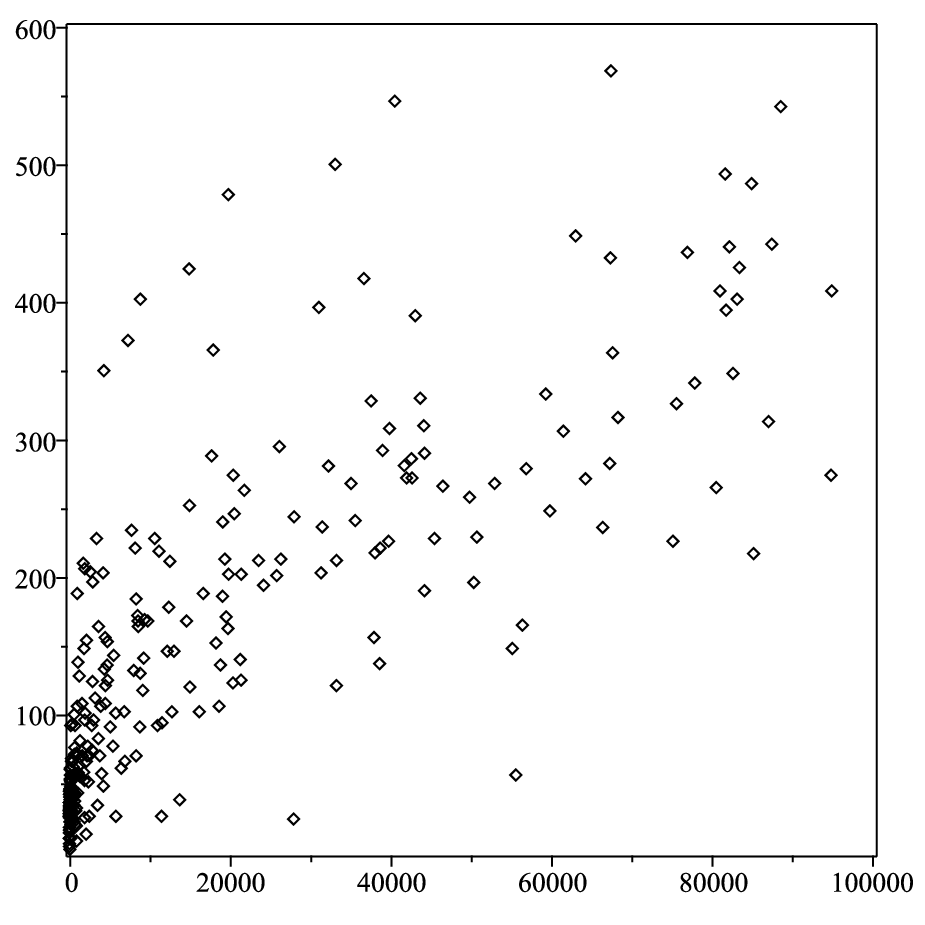
As shown in Fig. 2, the vast majority of the models have a very large parameter several orders of magnitude above 1, suggesting that warping corrections are far from being under control.
There are however also a few models with . In particular, out of the 605 models we studied, 11 admit a smaller than 10. The five models with the smallest are
| ID | CY | ||||||||||||
|---|---|---|---|---|---|---|---|---|---|---|---|---|---|
| NL1 | |||||||||||||
| NL2 | |||||||||||||
| NL3 | |||||||||||||
| NL4 | |||||||||||||
| NL5 |
Here “NL” means that the D7/O7 tadpoles are cancelled non-locally (see Section 5.3 for models with local tadpole cancelation).
One might wonder whether these models with can be marginally ok regarding the warping corrections. An interesting observation in this context is that smaller warping corrections correlate with smaller tadpoles. In Fig. 2, this is shown for the subset of models with and for a larger subset with . As we will discuss in Section 5.2, we therefore expect that there is a trade-off between control and consistent moduli stabilization. In particular, the models in the above table have tadpoles and should therefore be taken with a grain of salt. Recall that these are the upstairs tadpoles, i.e., they are even smaller by a further factor 2 on the orientifold.
Let us also remark that the T-branes in the NL1 and NL2 models have a negative Euler number and, as a consequence, contribute a positive D3 charge to the tadpole. This is quite unusual since D7-branes and O7-planes typically contribute negative D3 charges and thus act like O3-planes in the tadpole condition. Although we do not see an inconsistency with a negative per se3434 34 Nef divisors satisfy and [129] and therefore but this is not necessarily true for effective divisors., it suggests that is not a good proxy for the warping corrections in these models since it estimates the backreaction to be proportional to . Since the positive D3 charge of the T-brane and the negative D3 charges of the other localized sources do not locally cancel in these models, it is unclear why the warping should only be sensitive to the difference between these charges. As explained in Section 4.1, a more plausible estimate is that the backreaction is proportional the total negative D3 charge (or, equivalently, the total positive one). This suggests that one should use a modified proxy in these models in which is replaced by which does not contain the T-brane contribution. If one measures the warping corrections using this modified proxy in the NL1 and NL2 models, one finds , which is somewhat larger than the bound obtained using .
Regardless of which proxy one prefers to estimate the corrections, our analysis in any case suggests that LVS dS vacua with T-brane uplifting can at best lie at the boundary of control where the LVS potential becomes highly sensitive to the precise numerical coefficients of the warping corrections, in sharp contrast with the common belief of an exponentially small control parameter (cf. the discussion in Section 4.1).

5.2 Tuning Problem for Small Tadpoles
As discussed above, the models with the smallest (and thus the best control over warping corrections) have quite small tadpoles . Let us now elaborate a bit more on why this may be problematic. The crucial point is that the LVS is based on the assumption that the axio-dilaton, the complex-structure moduli and the brane moduli are stabilized by fluxes and that this happens in such a way that and take precisely the values required for a dS minimum.
One may wonder whether a possible obstacle to this assumption is the tadpole conjecture [130], which postulates that has to satisfy a certain lower bound that depends linearly on the number of stabilized moduli. However, there is no strong motivation to consider the tadpole conjecture in our context since it is known that the bound can be violated in compactifications with non-Abelian gauge groups and/or [131, 132, 133, 134, 135].3535 35 The proposed bound is also violated in compactifications with a small number of moduli [136] and in non-geometric examples [137, 138, 139, 140]. The T-brane models studied in this paper have both of these features which suggests that small tadpoles can in principle be fine.
However, it is not sufficient to stabilize the axio-dilaton and the complex-structure moduli anywhere in the moduli space. Instead, a trustworthy type IIB description requires since otherwise the genus expansion breaks down, leading to large loop and instanton corrections and also large backreaction corrections from the D7-branes and O7-planes. Recall further from Sections 2.1 and 4.1 that the uplift parameter lies in the interval in a dS vacuum and that we should not come too close to the boundaries of this interval since otherwise either corrections to the vacuum energy or the Hessian blow up. Hence, is fixed up to a few percent, which corresponds to a very thin band in the -plane. Stabilizing the moduli such that we land within this band is expected to require a certain amount of fine-tuning. This is only possible if there is enough freedom in choosing the fluxes or, in other words, if is not too small.
To be more concrete, note that (2.7), (2.8) and (3.1) imply
| (5.2) |
up to subleading terms in , where we also used the tadpole condition . We further defined in order to make explicit the dependence of due to a curvature correction to the instanton/D7-brane action which is proportional to the Euler number of the small divisor.
In a given Calabi-Yau orientifold model, we thus have for some fixed numbers , . Hence, for in the dS range and a given choice of , is fixed up to a few percent. According to (4.11), the allowed parameter region is in addition bounded by
| (5.3) |
Note that this inequality is automatically satisfied in every flux vacuum in which the complex-structure moduli and the axio-dilaton are stabilized supersymmetrically. The only tuning requirements on , are therefore hitting the small-coupling regime and the dS region.
As an example, consider the model NL4 of Section 5.1, which corresponds to the parameter choices , , , , , . As is standard in the literature, we also assume for concreteness. Using these values in the above expressions, we find
| (5.4) |
The resulting dS region in the -plane is plotted in Fig. 3. As anticipated, this region is indeed a very thin band, suggesting that landing in it requires some freedom in the fluxes and, accordingly, a not too small tadpole. Note that the dS region satisfies so that the requirement of a small string coupling does not lead to an additional constraint in this case.
To summarize, we expect that consistent dS vacua require an at least moderately large tadpole (even assuming that the tadpole conjecture does not apply in our context). This suggests that the naively best-controlled solutions in Section 5.1 may have to be discarded and that the control problems observed there would become even worse.
In principle, constructing Calabi-Yau orientifolds with very large tadpoles is not a problem, as emphasized, e.g., in [107]. However, we have seen that, in LVS models with a T-brane uplift, there is a trade-off between achieving control over warping/ corrections on the one side and large on the other side. This did not have to be the case: although it naively seems obvious that making large will also make large, this is not necessarily true since the vev of may a priori depend non-trivially on the fluxes. For the anti-brane uplift, one indeed finds that tends to get smaller in dS solutions with larger tadpoles because then there is more freedom to find solutions with large volumes [7, 8]. For the T-brane uplift, it is the other way round, i.e., we cannot obtain large and small at the same time.
5.3 Local Tadpole Cancelation
As explained in Section 4.3, models with non-local D7/O7 tadpole cancelation have the disadvantage that, regardless of how small is, there are in any case unsuppressed dilaton-backreaction corrections which modify the vev of the volume modulus by factors. Whether or not this is a serious problem is debatable but let us in any case discuss what happens if we demand local tadpole cancelation as an additional constraint.
Since, by assumption of the scenario, we have a stack of D7-branes on , canceling their tadpole locally means that we require O7-planes on as well and therefore we have to set . In order to cancel the tadpole of the T-brane, we furthermore require an O7-plane wrapping or a multiple thereof, i.e., . The only possibility consistent with is in our models, cf. App. B. With this orientifold choice, the T-brane stack must then wrap for local tadpole cancelation, i.e., we have , . The constraint (2.38) further implies , and the tadpole conditions (2.58) yield . In summary, demanding that O7/D7 charges cancel locally amounts to the parameter choices
| (5.5) |
As shown in App. B, only five of the 11 Calabi-Yau manifolds in our list admit an orientifolding with . Since the brane configuration (i.e., the choice for , and ) is unique, this means that only five of the 605 T-brane models we scanned have local tadpole cancelation. Using (5.5), we find that these models have the following properties:
| ID | CY | |||||
|---|---|---|---|---|---|---|
| L1 | ||||||
| L2 | ||||||
| L3 | ||||||
| L4 | ||||||
| L5 |
We thus see that in all models with local D7/O7 tadpole cancelation, suggesting that warping corrections are far from being under control. Furthermore, the D3 tadpoles are relatively small in all models. This is perhaps not surprising, as the D3 tadpole in the local case is known to be much more constrained than in the non-local case [107].
6 Models with
So far, our focus was on models with . Let us now move on to the case . We will not perform an exhaustive analysis in this section but only make a few observations. We consider a Swiss-cheese Calabi-Yau with small divisors such that
| (6.1) |
where we denote the volumes of the small divisors by and their triple-intersection numbers by with . We further assume that each of the small divisors hosts a non-perturbative effect leading to a superpotential
| (6.2) |
For simplicity, we will consider the situation where , and take the same values for all and where all are stabilized at the same value. Writing
| (6.3) |
one then finds that the volume and the superpotential take the same form as in the case:
| (6.4) |
One furthermore verifies that the scalar potential is given by (2.6) and so also takes the same form as for .
This implies in particular that the bound (3.1) on holds for arbitrary , with the caveat that in the bound now refers to the “effective” triple-intersection number defined in (6.3). Since and the bound on scales inversely with , one may naively think that the bound is relaxed at large . However, the bound also depends on , which gets smaller for larger (since ). Furthermore, the warping corrections we want to minimize do not only depend on the volume but also on the tadpole which is expected to get larger when many cycles are present on which D7-branes/O7-planes can contribute. It is therefore a priori unclear whether large makes the problem with the warping corrections better or worse. We will refrain from a general analysis of this question here since there is a more immediate problem with large . Indeed, the volumes of the small divisors satisfy
| (6.5) |
up to subleading corrections. This scaling behavior with respect to was already pointed out in [45]. However, unlike that reference, we view this as problematic since at large . Because of (2.7), it is unclear how to ensure a large volume in this regime. We also expect to lose control over the instanton expansion since so that higher-rank instantons contributing to the superpotential are in danger of dominating over the lowest-rank ones. Similarly, the (curvature-corrected) gauge kinetic function of a D7-brane wrapping one of the small divisors has the wrong sign at large , Re. Finally, another possible problem are loop corrections [109], which may blow up for . For these various reasons, we do not think that large can lead to viable models.
Let us therefore now consider the case where is a bit larger than 2 but not too large. We will not perform a systematic scan of such manifolds here but only discuss two explicit examples with . The first example was worked out and found to have dS vacua in [45]. We refer to [45] for the details of the toric construction and only state the topological data relevant for us:
| (6.6) |
where the bound on arises because the model of [45] does not have a D7 stack wrapped on and therefore the non-perturbative effect is due to instantons.
Furthermore, the volume of one of the small divisors is taken to zero in [45] in order to be able to place D3-branes at a singularity. In this limit, does not appear in the volume anymore so that there are effectively only two small divisors to be stabilized, i.e., . Each of these divisors is del Pezzo and hosts a non-perturbative effect. Hence, we can use the bound derived in Section 3 if we take for the effective intersection number
| (6.7) |
Plugging this into (3.2), we find
| (6.8) |
Hence, the string-frame volume is very small in any dS vacuum and we do not expect that and warping corrections are under control.3636 36 As mentioned in Section 2.5, our uplift term differs from the one used in [45] by a factor . Using the uplift term of [45], we would obtain a somewhat larger (but still quite small) bound, namely . This latter bound is consistent with the Einstein-frame volumes listed in (45, Table 4) after converting them to the string frame.
We also note that the curvature-corrected instanton actions on the small divisors are negative in this example,
| (6.9) |
where we used (6.5) and that for a del Pezzo divisor. As explained above, this suggests that the instanton expansion may not be under control.
A very similar model, which also has , was studied in [44]. The relevant topological data are
| (6.10) |
As in the previous model, the divisor volume is taken to zero so that, from the point of view of moduli stabilization, we effectively have one big and two small divisors, i.e., . The effective triple-intersection number is thus
| (6.11) |
A subtlety in this model is that, contrary to all other models discussed in this paper, and are not an integral basis of , which has the consequence that the flux on the T-brane is not bounded by but , as explained in [44] (see also our discussion in Section 2.4). Using these data in (3.1), we obtain
| (6.12) |
Hence, we again find a very small string-frame volume.3737 37 As mentioned in Section 2.5, our uplift term differs from the one used in [44] by a factor . Using the uplift term of [44], we would obtain a somewhat larger (but still quite small) bound, namely . However, this latter bound is still at odds with (44, Table 1), which yields much larger values when converting the Einstein-frame volumes displayed there to the string frame. The remaining discrepancy seems to originate from a disagreement between (44, Table 1) and (44, (4.27)) when plugging in the corresponding values of and (in the notation of [44]). We also again observe in this model that the instanton action is negative,
| (6.13) |
where we used (6.5) and that .
In summary, we argued that the control problems of the T-brane uplift are likely to be present on manifolds with as well, and we analyzed two explicit examples in which this indeed turns out to be the case.
7 Comments on Brane-moduli Stabilization
In this section, we discuss a potential problem with – or rather a challenge for – the stabilization of the D7-brane moduli in vacua with T-branes. This problem is independent of the control problems discussed in the previous sections, i.e., it would occur even in (hypothetical) solutions without large or warping corrections. It also does not depend on the vacuum energy and so occurs for dS, Minkowski and AdS.
Our main point is that the combined -term and -term potential for derived in Section 2.5 leaves many of the brane moduli unstabilized. This is a source of concern since any unknown correction, regardless of how small it is, can destabilize these moduli and possibly lead to decays to other configurations or runaways towards uncontrolled regimes. To see the problem, consider for simplicity the case , i.e., a stack of two D7-branes on with gauge group USp SU. As explained in Section 2.2, we can then decompose the field as
| (7.1) |
where the ’s are harmonic -forms (with respect to an appropriate gauge-covariant derivative operator) and the subscripts indicate that they are orientifold-even or odd. Expanding this into cohomology classes yields
| (7.2) |
Here, , , and are complex moduli with indices , , and . Note that denotes the cohomology group of -forms valued in the line bundle and the subscripts stand for orientifold-even/odd as before. The ’s are harmonic -forms which are a basis of or complex conjugate to a basis of , respectively. We will ignore the Wilson-line moduli for simplicity (see [69] for more details), which are counted by and and should in principle also be stabilized.
Substituting (7.2) into (2.39), (2.42), we obtain the potential
| (7.3) |
where and
| (7.4) |
The first line in (7.3) comes from the -term potential (2.39) and the second line is the contribution from the -term potential (2.42). Note that (7.3) reduces to our earlier potential (2.45) if we set all fields except to zero and consider a collective mode with .
Assuming the -term part of the potential (7.3) is steep enough (), there are extrema with satisfying
| (7.5) |
These are precisely the T-brane vacua we have been discussing throughout this paper. We thus see that the , and moduli are all stabilized at the origin but only a single real combination of the moduli is stabilized. The remaining real combinations are unstabilized. Although we focussed on the SU case here, it is clear that similar conclusions also apply for brane stacks with other gauge groups.
One may try to resolve this problem by turning on terms in the superpotential that depend on the moduli. Recall that we assumed that the superpotential does not depend on the brane moduli (following [43, 44, 45]) since this was sufficient for the purpose of generating the uplift term. A superpotential can in principle be generated in several different ways: by turning on -form worldvolume fluxes [81, 71, 141, 90], by D7/O7 backreaction effects [141, 65, 93] or by instanton corrections whose Pfaffian prefactors depend on the brane moduli [106].
Consistency of the -term requires that the superpotential is gauge-invariant [142] (see also [43]), i.e.,
| (7.6) |
must hold for all moduli values. Here, is the U charge of (with respect to the U along which we turned on the worldvolume flux) and we used that the and moduli have U charges (since they are the coefficients of bundle-valued -forms). The above constraint is satisfied, e.g., for polynomial terms
| (7.7) |
or non-perturbative terms
| (7.8) |
with . It would be important to understand to what extent such terms can be generated in the superpotential without significantly affecting the uplift mechanism explained in Section 2.5. Alternatively, a potential for the ’s might also be generated by corrections in the Kähler potential. As stated before, all of these possibilities may in principle go either way: they could stabilize or destabilize the moduli. We leave a detailed analysis of such questions for future work. In any case, even if the moduli-stabilization issue turns out to be merely a technical challenge rather than a serious obstacle, we believe that the control problem pointed out in the earlier sections of this paper is by itself already severe enough to invalidate the consistency of T-brane-uplifted dS vacua.
8 Conclusion
In this paper, we studied dS vacua obtained through a T-brane uplift in the LARGE-volume scenario (LVS). Since the LVS with anti-brane uplift is known to have control issues [6, 7, 8, 9, 10, 11, 12], a natural suspicion is that similar problems occur for the T-brane uplift as well, and we indeed found this to be the case.
We emphasized that a controlled dS construction requires that corrections which are not explicitly computed must be shown to be suppressed by a small control parameter. Naively, the LVS provides an exponentially small control parameter for both and warping corrections, namely the inverse of the volume. A common lore is that the volume is exponentially large in the LVS for moderately small and that therefore the scenario is excellently controlled. However, we showed that the string-frame volume in T-brane-uplifted dS vacua is in fact bounded by a number which only depends on topological data of the Calabi-Yau orientifold and does therefore not have much tuning freedom. This bound immediately rules out large volumes in many models where the non-perturbative effect comes from D3-brane instantons. In such models, the string-frame volume is often of the order 1 in string units or even much smaller than that, implying that there is no control at all. We furthermore argued that the control parameter that potentially suppresses the warping corrections is not simply but contains other factors, in particular the tadpole , which can be large and thus cancel the naive volume suppression even in models with gaugino condensation where our bound admits relatively large volumes and would thus naively not be that worrisome. Explicitly, we argued that a plausible proxy for controlling warping corrections is the condition .
In order to assess whether this condition can be satisfied in T-brane-uplifted dS vacua, we performed a detailed study of eleven Swiss-cheese Calabi-Yau manifolds with that can be constructed from the Kreuzer-Skarke list. We constructed all orientifolds of these manifolds which arise from reflection involutions with respect to the irreducible divisors of the ambient toric variety, resulting in 28 different Calabi-Yau orientifolds suitable for the LVS. We then computed all possible D-brane and flux configurations yielding a T-brane uplift in these orientifolds, leading in total to different models with a T-brane uplift and candidate dS vacua.
Our analysis showed that, while large volumes are indeed possible in these models, the volumes are never large enough to allow a suppression of the warping corrections, assuming they are reliably estimated by our proxy . Indeed, in all models we studied, so that we expect large warping corrections to the vacuum energy and the moduli masses. In fact, we found that the majority of the models have a huge several orders of magnitude above 1 and only a handful of models has a near the boundary of control . Another interesting observation was that the latter models have very small tadpoles with (upstairs). This raises the question whether the axio-dilaton and all complex-structure moduli can consistently be stabilized in these models and at the same time , can be fine-tuned such that a dS vacuum is obtained. If this is not the case, the true lower bound on is much larger than , increasing the control problems even more.
The problems we found have been overlooked previously due to a combination of reasons: First, our analysis revealed that previous derivations of the uplift term missed a factor (which counts the number of D7-branes combining into the T-brane). The stabilized volume in a dS vacuum scales with this factor like and is thus highly sensitive to it. Second, many papers studying the LVS only compute the Einstein-frame volumes of the claimed dS solutions, but the relevant parameter for controlling corrections is the string-frame one, which is by a factor smaller. This is in particular true for corrections. Also the warping corrections we studied are not suppressed by as one might have expected but actually only by due to the non-perturbative no-scale structure [6] of the LVS potential. Third, we argued that the warping corrections do not only scale with the inverse volume but also with the tadpole which tends to cancel any naive volume suppression that might arise. Hence, compared to what one might have guessed, the warping corrections are larger by a factor and thus much more dangerous than previously anticipated.
Another interesting observation, which we only discussed very briefly, is that there is a second type of corrections which mimicks the parametric behavior of the warping corrections but has a completely different origin, namely curvature corrections in the worldvolume theory of the D7-branes. This dual-threat situation is reminiscent of the anti-brane uplift where similarly not only warping corrections in the bulk but also local curvature corrections on the anti-brane can lead to control problems, as pointed out in [6] and further studied in [8, 9, 10, 11].
In the last section of this paper, we also briefly discussed an additional challenge for vacua with T-branes, namely that some of the brane moduli are left unstabilized if one follows the assumptions of the original scenario. This challenge is independent of the control problems for dS vacua and needs to be addressed in any putative T-brane vacuum, regardless of the sign of the vacuum energy.
Regarding future work, it would be interesting to elaborate on several aspects of the issues raised in this paper. For one thing, it would be interesting to perform a more detailed study of Calabi-Yau manifolds with . We already gave an argument that large does not lead to controlled vacua and moreover analyzed two explicit models with constructed previously in [44, 45], which we found to have very small volumes. Nevertheless, it is possible that there are other models with in which the control problems observed in this paper are somewhat relaxed. It would be nice to prove a general lower bound on which either rules out the existence of controlled models entirely for all or instead gives a concrete hint which properties are needed to achieve an at least smallish . It would also be interesting to study setups with more general worldvolume fluxes, in particular by allowing elements of which are not pulled back from . Identifying all such fluxes is a non-trivial task but may lead to interesting effects, e.g., a somewhat different quantization of the flux numbers , (which may affect the size of the uplift term) and the generation of a superpotential for the brane moduli (which may resolve the stabilization challenge discussed in Section 7).
More generally, given that control over warping and curvature corrections seems to be a prevalent issue in many different dS scenarios, it would also be important to make progress on computing such corrections explicitly. Instead of having to suppress them, one could then incorporate them into the potential and check whether the corrected potential still admits dS vacua. For the warping corrections, this requires a computation of the Green’s function of the Laplacian with respect to the Calabi-Yau metric. In toroidal orbifold limits, this can be done explicitly [143, 144, 145]. Recent progress for smooth metrics was made in [146].
Finally, we find it quite striking that very similar control problems seem to exist in the different variants of the LVS with T-brane and anti-brane uplift and also in other scenarios like KKLT, classical dS models and even supercritical dS models which are technically quite different from the LVS. In our view, this strongly suggests an underlying principle that string theory does not like dS vacua, at least in the computationally accessible weakly curved regime, and it would clearly be important to understand on general grounds if and why such a principle could be true.
Acknowledgments
I would like to thank Christoph Mayrhofer for a useful discussion. This research was funded by the German Research Foundation (Deutsche Forschungsgemeinschaft) under the project number 516370439.
Appendix A Normalization of the T-brane Uplift
In this appendix, we verify the normalization of the uplift term generated by the T-brane. To this end, the following kinetic and potential terms in the 4d effective field theory are relevant:
| (A.1) |
Recall that and are matrices whose entries are 2-forms on the divisor . We furthermore denote by the pullback onto that divisor.
Without loss of generality, we normalize such that, in 4d Planck units,
| (A.2) |
In [69], the -term potential of a non-Abelian D7 stack was derived by dimensionally reducing the DBI action. The result is
| (A.3) |
The -term potential generated by the D7-branes was also derived in [69] by dimensional reduction, yielding
| (A.4) |
An alternative is to determine using the Kähler potential. For a single brane and assuming , one has [64]
| (A.5) |
where the axio-dilaton is defined as , and the ’s are the complex-structure moduli. This expression is valid up to various corrections (e.g., terms of higher orders in and ) which we neglect here. Also note that should be viewed as a function of the 4d moduli. For a single brane, we can write in terms of complex moduli and some basis of harmonic -forms. For brane stacks with , one has to expand in certain bundle cohomologies, see [69] for an extensive discussion. Spelling out the moduli dependence explicitly is then rather cumbersome (cf. Section 7) so that it is more convenient to keep it implicit in the following.
A key assumption of the LVS is that integrating out and the ’s is equivalent to setting them to constants in the superpotential and Kähler potential. As explained in [57, 58], this is justified if these moduli approximately decouple from the Kähler and brane moduli. This is indeed the case in the regime of small we are interested in: Although solving yields -dependent vevs for , due to the mixing in (A.5), taking this into account only gives subleading corrections of the order to the kinetic terms. The same is true in the -term potential. Indeed, one can check that taking into account the dependence of the , vevs yields terms of the order , whereas we will see momentarily that the leading terms depending on are of the order . Hence, also here the mixing is negligible. Note that we assume that the mixing comes purely from (A.5). In particular, we adopt the assumption of [43] and subsequent works on T-brane uplifting that the superpotential is independent of .3838 38 As discussed in Section 7, turning on a superpotential for the brane moduli may help to stabilize them but can at the same time affect the uplift term. One would furthermore have to redo the check of the decoupling approximation in that case.
We can therefore neglect the mixing between and the bulk moduli and set them to constants. Hence, after integrating out and the ’s, the Kähler potential for is
| (A.6) |
Here, is an arbitrary constant which can be set to any value by a field rescaling. In the following, we set since this normalizes such that its kinetic term agrees with (A.1), (A.2). Furthermore, the natural generalization from the single-brane case to a brane stack is to put a trace in front of the Kähler potential. We thus arrive at
| (A.7) |
This is indeed confirmed in [69].
We now consider the -term potential, which in 4d Planck units is . Since, by assumption of the LVS, and the ’s are stabilized supersymmetrically, the index only runs over the Kähler and brane moduli. One can check that all terms involving derivatives with respect to the Kähler moduli cancel with the term due to the well-known no-scale structure, up to terms whose dependence is negligibly small. The leading -term potential for is given by where now only runs over the brane moduli. Since the superpotential is independent of by assumption of the scenario, we have
| (A.8) |
where we used , and at the quadratic order in . Comparing to (A.1), we conclude
| (A.9) |
in agreement with the (more general) result of [69]. We have thus fixed the coefficient of the -term potential in (A.1) without having to derive it directly from the D7-brane action. This is possible due to the fact that the coefficients of the kinetic term and the -term potential for are both determined by the Kähler potential, i.e., is fixed by the structure of 4d supergravity once we choose .
Appendix B Swiss-Cheese Calabi-Yau Orientifolds with
In this appendix, we provide some details on the Swiss-Cheese Calabi-Yau manifolds used in our scan in Section 5. Aside from stating their relevant topological data, we determine all orientifolds of these manifolds which are obtained by reflection involutions of the form
| (B.1) |
on one of the projective coordinates of the ambient variety . Such involutions have codimen-sion-1 and codimension-3 fixed loci on , i.e., O7-planes and O3-planes. We compute, for each involution, the invariant locus of the O7-plane and the O3-plane number . We discard an orientifold if since then tadpole cancelation implies that we cannot put a T-brane on . We also perform a few consistency checks to identify possible singularities of the orientifold-invariant Calabi-Yau hypersurfaces. In particular, we verify that the number of complex-structure moduli is integral in all orientifolds we keep. We further observe that a singularity is signaled when codimension-3 fixed loci of the orientifold involution appear to have fractional O3-plane numbers or when codimension-1 fixed loci appear to have fractional O7-plane numbers. We show that both phenomena are indeed related to singularities in several examples and discard orientifolds exhibiting such a behavior. An exhaustive analysis of all possible singularities is beyond the scope of this work so that some of the orientifolds we keep may still have more subtle singularities missed by our checks. See also [107] for a related discussion.
B.1
The relevant topological data of the manifold are
| (B.2) |
The weight matrix is
| CY | ||||||
|---|---|---|---|---|---|---|
with Stanley-Reisner (SR) ideal . The irreducible toric divisors satisfy
| (B.3) |
up to linear equivalence. The divisor specifying the Calabi-Yau hypersurface is . Here and in the following, we denote by both the divisors on the ambient variety and their pullbacks onto .3939 39 Calabi-Yau manifolds can in principle have additional divisors that do not descend from the ambient space but this does not happen for the manifolds in this appendix. The condition ensuring this is called favorability, see, e.g., [124, 23] for discussions. According to the database of [124, 125], all Calabi-Yau manifolds with obtained from the Kreuzer-Skarke list are indeed favorable. Note that all divisors are linear combinations of the two linear equivalence classes , (as expected for ). Since these combinations are integral, , span an integral basis of , which is the case for all manifolds discussed in this appendix. Effective divisors are obtained by considering non-negative integer linear combinations of the ’s.
The possible orientifold choices are
| involution | viable? | |||
|---|---|---|---|---|
| I1/I2 | 45 | ✓ | ||
| I3 | × | |||
| I4 | × | |||
| I5 | × | |||
| I6 | × |
Let us explain how the various entries in the table are obtained. We first consider the case I1. Due to the projective identifications following from the weight matrix, the involution can equivalently be viewed as or . The fixed points are thus , and . One verifies that none of them lie in the SR ideal and all of them intersect with the Calabi-Yau hypersurface. They thus correspond to an O7-plane wrapped on and six O3-planes since . The I2 involution works analogously.
For the other involutions, it turns out that the requirement of orientifold invariance enforces singularities on the Calabi-Yau hypersurface. To see this, we first consider the I3 and I5 involutions. Using the projective identifications, one can show that both involutions have fixed points at . The associated number of O3-planes can naively be computed by intersecting the corresponding divisors, but this does not yield an integer, , suggesting a singularity. To see that this is indeed the correct interpretation, consider first a generic Calabi-Yau hypersurface in . The defining polynomial reads at . Since at due to the SR ideal, this implies . Hence, the fixed points do not intersect with a generic Calabi-Yau. However, for the I3 and I5 orientifolds, the term in is projected out so that now , i.e., the fixed points are located on the Calabi-Yau as soon as we impose orientifold invariance. At the same time, one also finds for all . Hence, both and its differential vanish at , which indicates that the hypersurface is singular there [107]. We thus see that the fractional O3-plane number is related to a singularity as anticipated. We therefore discard the I3 and I5 orientifolds.
We can repeat the analysis for the I4 and I6 involutions, which have fixed points at . The intersection number of the corresponding divisors is again fractional, , so that we again expect a singularity. For a generic Calabi-Yau, we have at . Since at due to the SR ideal, the fixed points lie outside of a generic Calabi-Yau. However, for the I4 and I6 orientifolds, the term in is projected out so that , . We thus conclude that the I4 and I6 orientifolds are singular as well and discard them.
B.2
The relevant topological data of the manifold are
| (B.4) |
The weight matrix is
| CY | ||||||
|---|---|---|---|---|---|---|
with SR ideal . The irreducible toric divisors satisfy
| (B.5) |
The divisor specifying the Calabi-Yau hypersurface is . Note that the above data are equivalent to upon exchanging , .
The possible orientifold choices are
| involution | viable? | |||
|---|---|---|---|---|
| I1/I2 | 45 | ✓ | ||
| I3 | × | |||
| I4 | × | |||
| I5 | × | |||
| I6 | × |
The singularity checks are analogous to , leading to the conclusion that the I3, I4, I5 and I6 orientifolds are singular.
B.3
The relevant topological data of the manifold are
| (B.6) |
The weight matrix is
| CY | ||||||
|---|---|---|---|---|---|---|
with SR ideal . The irreducible toric divisors satisfy
| (B.7) |
The divisor specifying the Calabi-Yau hypersurface is .
The possible orientifold choices are
| involution | viable? | |||
|---|---|---|---|---|
| I1 | 49 | ✓ | ||
| I2/I3 | 45 | ✓ | ||
| I4 | 49 | ✓ | ||
| I5 | × | |||
| I6 | 33 | ✓ |
Note that the I5 involution has fractional fixed points at and which are not in the SR ideal. For a generic Calabi-Yau, we would have at or . Since at due to the SR ideal, the fixed points would lie outside of a generic Calabi-Yau. However, for the I5 orientifold, the term in is projected out so that , . We thus conclude that the I5 orientifold is singular.
B.4
The relevant topological data of the manifold are
| (B.8) |
The weight matrix is
| CY | ||||||
|---|---|---|---|---|---|---|
with SR ideal . The irreducible toric divisors satisfy
| (B.9) |
The divisor specifying the Calabi-Yau hypersurface is .
The possible orientifold choices are
| involution | viable? | |||
|---|---|---|---|---|
| I1 | × | |||
| I2/I3/I4 | 52 | ✓ | ||
| I5 | 46 | ✓ | ||
| I6 | × |
Note that the I6 involution has fractional fixed points at which are not in the SR ideal. For a generic Calabi-Yau, we would have at . Since at due to the SR ideal, the fixed points would lie outside of a generic Calabi-Yau. However, for the I6 orientifold, the term in is projected out so that , . We thus conclude that the I6 orientifold is singular.
In addition, also the I1 orientifold is singular. Unlike in the I6 case, this is not related to a fractional O3-plane number but to a fractional O7-plane number. The fixed points of I1 are located at , and . The first two sets correspond to an O7-plane wrapped on and three O3-planes, but the interpretation of the last one is less clear. Naively, one might think that it is an O5-plane since it arises at the intersection of and , which would have codimension 2 on a generic Calabi-Yau. However, on the orientifold-invariant Calabi-Yau, this degenerates to a codimension-1 surface and singularities appear.
To see this, consider again a generic Calabi-Yau first. We then have at , where , , are degree-5 and degree-4 polynomials of , , . It follows that
| (B.10) |
Since and cannot all vanish at due to the SR ideal, at least one of the above expressions is non-zero on a generic Calabi-Yau. On the other hand, for the I1 orientifold, the term is projected out in so that all expressions in (B.10) vanish at . Note that this in general has solutions with and is therefore not excluded by the SR ideal. We can therefore conclude that the Calabi-Yau has singularities in the I1 case. One can further check that and do not intersect transversally but in a codimension-1 surface on the invariant Calabi-Yau. This surface can however not be identified with a divisor on , as already suggested by applying the naive formula , which looks like a fractional O7-plane. An analogous problem can be shown to arise for the I6 orientifold (which we already excluded above) at . Below, we will furthermore observe the same behavior for some orientifolds of .
B.5
The relevant topological data of the manifold are
| (B.11) |
The weight matrix is
| CY | ||||||
|---|---|---|---|---|---|---|
with SR ideal . The irreducible toric divisors satisfy
| (B.12) |
The divisor specifying the Calabi-Yau hypersurface is .
The possible orientifold choices are
| involution | viable? | |||
|---|---|---|---|---|
| I1/I2/I3 | 51 | ✓ | ||
| I4 | 55 | ✓ | ||
| I5 | 55 | ✓ | ||
| I6 | × |
Note that the I6 involution has fractional fixed points at and which are not in the SR ideal. For a generic Calabi-Yau, we would have at . Since at and , cannot both vanish due to the SR ideal, the fixed points would lie outside of a generic Calabi-Yau. However, for the I6 orientifold, the term in is projected out so that , . We thus conclude that the I6 orientifold is singular.
B.6
The relevant topological data of the manifold are
| (B.13) |
The weight matrix is
| CY | ||||||
|---|---|---|---|---|---|---|
with SR ideal . The irreducible toric divisors satisfy
| (B.14) |
The divisor specifying the Calabi-Yau hypersurface is .
The possible orientifold choices are
| involution | viable? | |||
|---|---|---|---|---|
| I1 | 59 | ✓ | ||
| I2/I3/I4/I6 | 55 | ✓ | ||
| I5 | 59 | ✓ |
We did not observe singularities for any of the involutions on this manifold.
B.7
The relevant topological data of the manifold are
| (B.15) |
The weight matrix is
| CY | ||||||
|---|---|---|---|---|---|---|
with SR ideal . The irreducible toric divisors satisfy
| (B.16) |
The divisor specifying the Calabi-Yau hypersurface is .
The possible orientifold choices are
| involution | viable? | |||
|---|---|---|---|---|
| I1 | × | |||
| I2/I3/I4 | 54 | ✓ | ||
| I5 | × | |||
| I6 | × |
Note that the I6 involution has fractional fixed points at which are not in the SR ideal. For a generic Calabi-Yau, we would have at . Since at due to the SR ideal, the fixed points would lie outside of a generic Calabi-Yau. However, for the I6 orientifold, the term in is projected out so that , . We thus conclude that the I6 orientifold is singular.
We also find that the I1 and I5 orientifolds are singular. This is related to fractional O7-planes, analogously to what we discussed for . For I1, the orientifold involution has fixed points at and . The latter would be a codimension-2 surface on a generic Calabi-Yau and thus naively corresponds to an O5-plane. However, on the orientifold-invariant Calabi-Yau, the surface degenerates and becomes singular. For a generic Calabi-Yau, we have at , where the ’s are degree- polynomials in , , . Hence,
| (B.17) |
These expressions cannot all vanish generically due to the SR ideal. However, for the I1 orientifold, the term in is projected out so that all expressions vanish at . This can be solved for and thus does not lie in the SR ideal. We thus conclude that the I1 orientifold is singular. As in the examples, the singularity is signaled by the fact that the fixed locus is not given by an O7-plane wrapping an integral divisor on since . The discussion of the I5 orientifold is analogous, where the problematic fixed locus is now at .
B.8
The relevant topological data of the manifold are
| (B.18) |
The weight matrix is
| CY | ||||||
|---|---|---|---|---|---|---|
with SR ideal . The irreducible toric divisors satisfy
| (B.19) |
The divisor specifying the Calabi-Yau hypersurface is .
The possible orientifold choices are
| involution | viable? | |||
|---|---|---|---|---|
| I1/I2 | 64 | ✓ | ||
| I3 | 68 | ✓ | ||
| I4 | × | |||
| I5 | 68 | ✓ | ||
| I6 | 116 | ✓ |
Note that the I4 involution has fractional fixed points at and which are not in the SR ideal. For a generic Calabi-Yau, we would have at and at . Since at and , cannot both vanish due to the SR ideal, it follows so that the fixed points would lie outside of a generic Calabi-Yau. However, for the I4 orientifold, the and terms in are projected out so that , . We thus conclude that the I4 orientifold is singular.
B.9
The relevant topological data of the manifold are
| (B.20) |
The weight matrix is
| CY | ||||||
|---|---|---|---|---|---|---|
with SR ideal . The irreducible toric divisors satisfy
| (B.21) |
The divisor specifying the Calabi-Yau hypersurface is .
The possible orientifold choices are
| involution | viable? | |||
|---|---|---|---|---|
| I1 | 64 | × | ||
| I2/I3 | 68 | ✓ | ||
| I4 | × | |||
| I5 | × | |||
| I6 | 120 | ✓ |
Note that the I1 and I6 involutions have fractional fixed points at which are not in the SR ideal. For a generic Calabi-Yau, we have at . Since at due to the SR ideal, the fixed points lie outside of a generic Calabi-Yau. The same is true for the orientifolds since the term is not projected out. Hence, we cannot conclude on a singularity. However, we still exclude the I1 orientifold since it does not have an O7-plane on .
The I4 and I5 involutions have fractional fixed points at which are not in the SR ideal. For a generic Calabi-Yau, we would have at . Since at due to the SR ideal, the fixed points would lie outside of a generic Calabi-Yau. However, for the I4 and I5 orientifolds, the term in is projected out so that , . We thus conclude that the I4 and I5 orientifolds are singular.
B.10
The relevant topological data of the manifold are
| (B.22) |
The weight matrix is
| CY | ||||||
|---|---|---|---|---|---|---|
with SR ideal . The irreducible toric divisors satisfy
| (B.23) |
The divisor specifying the Calabi-Yau hypersurface is .
The possible orientifold choices are
| involution | viable? | |||
|---|---|---|---|---|
| I1/I2 | 70 | ✓ | ||
| I3 | × | |||
| I4 | 72 | ✓ | ||
| I5 | × | |||
| I6 | 128 | ✓ |
Note that the I3 and I5 involutions have fractional fixed points at which are not in the SR ideal. For a generic Calabi-Yau, we would have at . Since at due to the SR ideal, the fixed points would lie outside of a generic Calabi-Yau. However, for the I3 and I5 orientifolds, the term in is projected out so that , . We thus conclude that the I3 and I5 orientifolds are singular.
The I4 and I6 involutions have fractional fixed points at which are not in the SR ideal. For a generic Calabi-Yau, we have at . Since at due to the SR ideal, the fixed points lie outside of a generic Calabi-Yau. The same is true for the orientifolds since the term is not projected out. Hence, we cannot conclude on a singularity.
B.11
The relevant topological data of the manifold are
| (B.24) |
The weight matrix is
| CY | ||||||
|---|---|---|---|---|---|---|
with SR ideal . The irreducible toric divisors satisfy
| (B.25) |
The divisor specifying the Calabi-Yau hypersurface is .
The possible orientifold choices are
| involution | viable? | |||
|---|---|---|---|---|
| I1 | 78 | ✓ | ||
| I2/I3/I4 | 74 | ✓ | ||
| I5 | 78 | ✓ | ||
| I6 | 132 | ✓ |
There are no singularities related to fractional fixed points on this manifold. Note that the I6 involution has fractional fixed points at and which are not in the SR ideal. For a generic Calabi-Yau, we have at . Since at due to the SR ideal, the fixed points lie outside of a generic Calabi-Yau. The same is true for the orientifold since the term is not projected out. Hence, we cannot conclude on a singularity.
References
- (1) DESI Collaboration, A. G. Adame et al., DESI 2024 VI: cosmological constraints from the measurements of baryon acoustic oscillations, JCAP 02 (2025) 021 [2404.03002].
- (2) DESI Collaboration, M. Abdul Karim et al., DESI DR2 results. II. Measurements of baryon acoustic oscillations and cosmological constraints, Phys. Rev. D 112 (2025), no. 8, 083515 [2503.14738].
- (3) D. Andriot, Dark energy from string theory: an introductory review, 2603.25797.
- (4) V. Balasubramanian, P. Berglund, J. P. Conlon and F. Quevedo, Systematics of moduli stabilisation in Calabi-Yau flux compactifications, JHEP 03 (2005) 007 [hep-th/0502058].
- (5) J. P. Conlon, F. Quevedo and K. Suruliz, Large-volume flux compactifications: Moduli spectrum and D3/D7 soft supersymmetry breaking, JHEP 08 (2005) 007 [hep-th/0505076].
- (6) D. Junghans, LVS de Sitter vacua are probably in the swampland, Nucl. Phys. B 990 (2023) 116179 [2201.03572].
- (7) X. Gao, A. Hebecker, S. Schreyer and V. Venken, The LVS parametric tadpole constraint, JHEP 07 (2022) 056 [2202.04087].
- (8) D. Junghans, Topological constraints in the LARGE-volume scenario, JHEP 08 (2022) 226 [2205.02856].
- (9) A. Hebecker, S. Schreyer and V. Venken, Curvature corrections to KPV: do we need deep throats?, JHEP 10 (2022) 166 [2208.02826].
- (10) S. Schreyer and V. Venken, ’ corrections to KPV: an uplifting story, JHEP 07 (2023) 235 [2212.07437].
- (11) S. Schreyer, Higher order corrections to KPV: The nonabelian brane stack perspective, JHEP 07 (2024) 075 [2402.13311].
- (12) B. Valeixo Bento, D. Chakraborty, S. Parameswaran and I. Zavala, De Sitter vacua — when are ‘subleading corrections’ really subleading?, JHEP 11 (2023) 075 [2306.07332].
- (13) M. P. Hertzberg, S. Kachru, W. Taylor and M. Tegmark, Inflationary Constraints on Type IIA String Theory, JHEP 12 (2007) 095 [0711.2512].
- (14) E. Silverstein, Simple de Sitter Solutions, Phys. Rev. D 77 (2008) 106006 [0712.1196].
- (15) D. Junghans, Weakly Coupled de Sitter Vacua with Fluxes and the Swampland, JHEP 03 (2019) 150 [1811.06990].
- (16) A. Banlaki, A. Chowdhury, C. Roupec and T. Wrase, Scaling limits of dS vacua and the swampland, JHEP 03 (2019) 065 [1811.07880].
- (17) L. Horer and D. Junghans, Almost classical de Sitter?, JHEP 09 (2024) 038 [2406.01690].
- (18) D. Andriot and F. Ruehle, On classical de Sitter solutions and parametric control, JHEP 06 (2024) 101 [2403.07065].
- (19) S. Kachru, R. Kallosh, A. D. Linde and S. P. Trivedi, De Sitter vacua in string theory, Phys. Rev. D68 (2003) 046005 [hep-th/0301240].
- (20) F. Carta, J. Moritz and A. Westphal, Gaugino condensation and small uplifts in KKLT, JHEP 08 (2019) 141 [1902.01412].
- (21) X. Gao, A. Hebecker and D. Junghans, Control issues of KKLT, Fortsch. Phys. 68 (2020) 2000089 [2009.03914].
- (22) R. Blumenhagen, A. Gligovic and S. Kaddachi, Mass Hierarchies and Quantum Gravity Constraints in DKMM-refined KKLT, Fortsch. Phys. 71 (2023), no. 1, 2200167 [2206.08400].
- (23) L. McAllister, J. Moritz, R. Nally and A. Schachner, Candidate de Sitter vacua, Phys. Rev. D 111 (2025), no. 8, 086015 [2406.13751].
- (24) F. Farakos, G. Tringas and T. Van Riet, Warped -throats in IIA and uplift dSillusions, Eur. Phys. J. C 85 (2025), no. 9, 1018 [2505.21104].
- (25) E. Silverstein, (A)dS backgrounds from asymmetric orientifolds, Clay Mat. Proc. 1 (2002) 179 [hep-th/0106209].
- (26) A. Maloney, E. Silverstein and A. Strominger, De Sitter space in noncritical string theory, in Workshop on Conference on the Future of Theoretical Physics and Cosmology in Honor of Steven Hawking’s 60th Birthday. 5, 2002. hep-th/0205316.
- (27) D. Junghans, de Sitter-eating O-planes in supercritical string theory, JHEP 12 (2023) 196 [2308.00026].
- (28) S. Parameswaran and M. Serra, On (A)dS solutions from Scherk-Schwarz orbifolds, JHEP 10 (2024) 039 [2407.16781].
- (29) B. V. Bento and M. Montero, An M-theory dS maximum from Casimir energies on Riemann-flat manifolds, JHEP 01 (2026) 099 [2507.02037], [Erratum: JHEP 07, 191 (2026)].
- (30) M. Aparici, B. Valeixo Bento and M. Montero, A maximum in M-theory from Casimir energies on Riemann-flat manifolds, 2609.16169.
- (31) A. Hebecker, S. Lüst, A. Schachner and S. Schreyer, Effective potentials, warping, and implications for F-term uplifting, JHEP 05 (2026) 286 [2512.17995].
- (32) G. Obied, H. Ooguri, L. Spodyneiko and C. Vafa, De Sitter Space and the Swampland, 1806.08362.
- (33) H. Ooguri, E. Palti, G. Shiu and C. Vafa, Distance and de Sitter Conjectures on the Swampland, Phys. Lett. B 788 (2019) 180–184 [1810.05506].
- (34) S. K. Garg and C. Krishnan, Bounds on Slow Roll and the de Sitter Swampland, JHEP 11 (2019) 075 [1807.05193].
- (35) D. Andriot, On the de Sitter swampland criterion, Phys. Lett. B 785 (2018) 570–573 [1806.10999].
- (36) A. Hebecker and T. Wrase, The Asymptotic dS Swampland Conjecture - a Simplified Derivation and a Potential Loophole, Fortsch. Phys. 67 (2019), no. 1-2, 1800097 [1810.08182].
- (37) U. H. Danielsson and T. Van Riet, What if string theory has no de Sitter vacua?, Int. J. Mod. Phys. D 27 (2018), no. 12, 1830007 [1804.01120].
- (38) T. D. Brennan, F. Carta and C. Vafa, The String Landscape, the Swampland, and the Missing Corner, PoS TASI2017 (2017) 015 [1711.00864].
- (39) G. Dvali, C. Gomez and S. Zell, Quantum Break-Time of de Sitter, JCAP 06 (2017) 028 [1701.08776].
- (40) G. Dvali, C. Gomez and S. Zell, Quantum Breaking Bound on de Sitter and Swampland, Fortsch. Phys. 67 (2019), no. 1-2, 1800094 [1810.11002].
- (41) R. Donagi, S. Katz and E. Sharpe, Spectra of D-branes with higgs vevs, Adv. Theor. Math. Phys. 8 (2004), no. 5, 813–859 [hep-th/0309270].
- (42) S. Cecotti, C. Cordova, J. J. Heckman and C. Vafa, T-Branes and Monodromy, JHEP 07 (2011) 030 [1010.5780].
- (43) M. Cicoli, F. Quevedo and R. Valandro, De Sitter from T-branes, JHEP 03 (2016) 141 [1512.04558].
- (44) M. Cicoli, I. Garcia-Etxebarria, C. Mayrhofer, F. Quevedo, P. Shukla and R. Valandro, Global Orientifolded Quivers with Inflation, JHEP 11 (2017) 134 [1706.06128].
- (45) M. Cicoli, I. Garcia-Etxebarria, F. Quevedo, A. Schachner, P. Shukla and R. Valandro, The Standard Model quiver in de Sitter string compactifications, JHEP 08 (2021) 109 [2106.11964].
- (46) M. R. Douglas, The Statistics of string / M theory vacua, JHEP 05 (2003) 046 [hep-th/0303194].
- (47) S. Ashok and M. R. Douglas, Counting flux vacua, JHEP 01 (2004) 060 [hep-th/0307049].
- (48) F. Denef and M. R. Douglas, Distributions of flux vacua, JHEP 05 (2004) 072 [hep-th/0404116].
- (49) T. W. Grimm, Moduli space holography and the finiteness of flux vacua, JHEP 10 (2021) 153 [2010.15838].
- (50) B. Bakker, T. W. Grimm, C. Schnell and J. Tsimerman, Finiteness for self-dual classes in integral variations of Hodge structure, 2112.06995.
- (51) O. DeWolfe, A. Giryavets, S. Kachru and W. Taylor, Type IIA moduli stabilization, JHEP 07 (2005) 066 [hep-th/0505160].
- (52) P. G. Camara, A. Font and L. E. Ibanez, Fluxes, moduli fixing and MSSM-like vacua in a simple IIA orientifold, JHEP 09 (2005) 013 [hep-th/0506066].
- (53) C. Crinò, F. Quevedo and R. Valandro, On de Sitter String Vacua from Anti-D3-Branes in the Large Volume Scenario, JHEP 03 (2021) 258 [2010.15903].
- (54) F. Marchesano, R. Savelli and S. Schwieger, Compact T-branes, JHEP 09 (2017) 132 [1707.03797].
- (55) F. Marchesano, R. Savelli and S. Schwieger, T-branes and defects, JHEP 04 (2019) 110 [1902.04108].
- (56) S. B. Giddings, S. Kachru and J. Polchinski, Hierarchies from fluxes in string compactifications, Phys. Rev. D 66 (2002) 106006 [hep-th/0105097].
- (57) A. Achucarro, S. Hardeman and K. Sousa, Consistent Decoupling of Heavy Scalars and Moduli in N=1 Supergravity, Phys. Rev. D 78 (2008) 101901 [0806.4364].
- (58) D. Gallego and M. Serone, An Effective Description of the Landscape. I., JHEP 01 (2009) 056 [0812.0369].
- (59) K. Becker, M. Becker, M. Haack and J. Louis, Supersymmetry breaking and alpha-prime corrections to flux induced potentials, JHEP 06 (2002) 060 [hep-th/0204254].
- (60) R. Minasian, T. G. Pugh and R. Savelli, F-theory at order , JHEP 10 (2015) 050 [1506.06756].
- (61) S. Gukov, C. Vafa and E. Witten, CFT’s from Calabi-Yau four folds, Nucl. Phys. B 584 (2000) 69–108 [hep-th/9906070], [Erratum: Nucl.Phys.B 608, 477–478 (2001)].
- (62) K. Becker, M. Becker and A. Strominger, Five-branes, membranes and nonperturbative string theory, Nucl. Phys. B 456 (1995) 130–152 [hep-th/9507158].
- (63) M. Marino, R. Minasian, G. W. Moore and A. Strominger, Nonlinear instantons from supersymmetric p-branes, JHEP 01 (2000) 005 [hep-th/9911206].
- (64) H. Jockers and J. Louis, The Effective action of D7-branes in N = 1 Calabi-Yau orientifolds, Nucl. Phys. B 705 (2005) 167–211 [hep-th/0409098].
- (65) F. Denef, Lectures on constructing string vacua, Les Houches 87 (2008) 483–610 [0803.1194].
- (66) M. Demirtas, C. Long, L. McAllister and M. Stillman, The Kreuzer-Skarke Axiverse, JHEP 04 (2020) 138 [1808.01282].
- (67) R. Blumenhagen, V. Braun, T. W. Grimm and T. Weigand, GUTs in Type IIB Orientifold Compactifications, Nucl. Phys. B 815 (2009) 1–94 [0811.2936].
- (68) C. Beasley, J. J. Heckman and C. Vafa, GUTs and Exceptional Branes in F-theory - I, JHEP 01 (2009) 058 [0802.3391].
- (69) D. Junghans, -term and -term potential of non-Abelian D7-branes in IIB Calabi-Yau orientifolds, 2609.16136.
- (70) P. G. Camara, L. E. Ibanez and A. M. Uranga, Flux-induced SUSY-breaking soft terms on D7-D3 brane systems, Nucl. Phys. B 708 (2005) 268–316 [hep-th/0408036].
- (71) J. Gomis, F. Marchesano and D. Mateos, An Open string landscape, JHEP 11 (2005) 021 [hep-th/0506179].
- (72) E. G. Gimon and J. Polchinski, Consistency conditions for orientifolds and D-manifolds, Phys. Rev. D 54 (1996) 1667–1676 [hep-th/9601038].
- (73) M. R. Douglas and G. W. Moore, D-branes, quivers, and ALE instantons, hep-th/9603167.
- (74) A. Collinucci, F. Denef and M. Esole, D-brane Deconstructions in IIB Orientifolds, JHEP 02 (2009) 005 [0805.1573].
- (75) A. Collinucci, M. Kreuzer, C. Mayrhofer and N.-O. Walliser, Four-modulus ’Swiss Cheese’ chiral models, JHEP 07 (2009) 074 [0811.4599].
- (76) B. S. Acharya, M. Aganagic, K. Hori and C. Vafa, Orientifolds, mirror symmetry and superpotentials, hep-th/0202208.
- (77) I. Brunner and K. Hori, Orientifolds and mirror symmetry, JHEP 11 (2004) 005 [hep-th/0303135].
- (78) A. Sen, A Nonperturbative description of the Gimon-Polchinski orientifold, Nucl. Phys. B 489 (1997) 139–159 [hep-th/9611186].
- (79) A. Braun, A. Hebecker and H. Triendl, D7-Brane Motion from M-Theory Cycles and Obstructions in the Weak Coupling Limit, Nucl. Phys. B 800 (2008) 298–329 [0801.2163].
- (80) L. E. Ibanez, A. N. Schellekens and A. M. Uranga, Instanton Induced Neutrino Majorana Masses in CFT Orientifolds with MSSM-like spectra, JHEP 06 (2007) 011 [0704.1079].
- (81) H. Jockers and J. Louis, D-terms and F-terms from D7-brane fluxes, Nucl. Phys. B 718 (2005) 203–246 [hep-th/0502059].
- (82) M. Buican, D. Malyshev, D. R. Morrison, H. Verlinde and M. Wijnholt, D-branes at Singularities, Compactification, and Hypercharge, JHEP 01 (2007) 107 [hep-th/0610007].
- (83) T. W. Grimm, M. Kerstan, E. Palti and T. Weigand, On Fluxed Instantons and Moduli Stabilisation in IIB Orientifolds and F-theory, Phys. Rev. D 84 (2011) 066001 [1105.3193].
- (84) D. S. Freed and E. Witten, Anomalies in string theory with D-branes, Asian J. Math. 3 (1999) 819 [hep-th/9907189].
- (85) A. Collinucci and R. Savelli, On Flux Quantization in F-Theory, JHEP 02 (2012) 015 [1011.6388].
- (86) F. Denef and G. W. Moore, Split states, entropy enigmas, holes and halos, JHEP 11 (2011) 129 [hep-th/0702146].
- (87) C. Bachas, M. Bianchi, R. Blumenhagen, D. Lust and T. Weigand, Comments on Orientifolds without Vector Structure, JHEP 08 (2008) 016 [0805.3696].
- (88) F. Marchesano, R. Moraru and R. Savelli, A vanishing theorem for T-branes, JHEP 11 (2020) 002 [2007.02960].
- (89) M. Haack, D. Krefl, D. Lust, A. Van Proeyen and M. Zagermann, Gaugino Condensates and D-terms from D7-branes, JHEP 01 (2007) 078 [hep-th/0609211].
- (90) L. Martucci, D-branes on general N=1 backgrounds: Superpotentials and D-terms, JHEP 06 (2006) 033 [hep-th/0602129].
- (91) F. Marchesano, P. McGuirk and G. Shiu, Chiral matter wavefunctions in warped compactifications, JHEP 05 (2011) 090 [1012.2759].
- (92) F. Marchesano and S. Schwieger, T-branes and -corrections, JHEP 11 (2016) 123 [1609.02799].
- (93) M. Arends, A. Hebecker, K. Heimpel, S. C. Kraus, D. Lust, C. Mayrhofer, C. Schick and T. Weigand, D7-Brane Moduli Space in Axion Monodromy and Fluxbrane Inflation, Fortsch. Phys. 62 (2014) 647–702 [1405.0283].
- (94) F. Marchesano and L. Martucci, Non-perturbative effects on seven-brane Yukawa couplings, Phys. Rev. Lett. 104 (2010) 231601 [0910.5496].
- (95) E. Witten, Nonperturbative superpotentials in string theory, Nucl. Phys. B 474 (1996) 343–360 [hep-th/9604030].
- (96) R. Blumenhagen, M. Cvetic, S. Kachru and T. Weigand, D-Brane Instantons in Type II Orientifolds, Ann. Rev. Nucl. Part. Sci. 59 (2009) 269–296 [0902.3251].
- (97) J. Louis, M. Rummel, R. Valandro and A. Westphal, Building an explicit de Sitter, JHEP 10 (2012) 163 [1208.3208].
- (98) L. McAllister and F. Quevedo, Moduli Stabilization in String Theory, 2310.20559.
- (99) L. Gorlich, S. Kachru, P. K. Tripathy and S. P. Trivedi, Gaugino condensation and nonperturbative superpotentials in flux compactifications, JHEP 12 (2004) 074 [hep-th/0407130].
- (100) R. Kallosh and D. Sorokin, Dirac action on M5 and M2 branes with bulk fluxes, JHEP 05 (2005) 005 [hep-th/0501081].
- (101) M. Bianchi, A. Collinucci and L. Martucci, Magnetized E3-brane instantons in F-theory, JHEP 12 (2011) 045 [1107.3732].
- (102) M. Bianchi, G. Inverso and L. Martucci, Brane instantons and fluxes in F-theory, JHEP 07 (2013) 037 [1212.0024].
- (103) P. Berglund and I. Garcia-Etxebarria, D-brane instantons on non-Spin cycles, JHEP 01 (2013) 056 [1210.1221].
- (104) M. Cicoli, C. Mayrhofer and R. Valandro, Moduli Stabilisation for Chiral Global Models, JHEP 02 (2012) 062 [1110.3333].
- (105) D. Junghans, to appear.
- (106) R. Blumenhagen, S. Moster and E. Plauschinn, Moduli Stabilisation versus Chirality for MSSM like Type IIB Orientifolds, JHEP 01 (2008) 058 [0711.3389].
- (107) C. Crinò, F. Quevedo, A. Schachner and R. Valandro, A database of Calabi-Yau orientifolds and the size of D3-tadpoles, JHEP 08 (2022) 050 [2204.13115].
- (108) M. Cicoli, F. Quevedo, R. Savelli, A. Schachner and R. Valandro, Systematics of the Expansion in F-Theory, JHEP 2021 (2021) 99 [2106.04592].
- (109) X. Gao, A. Hebecker, S. Schreyer and V. Venken, Loops, local corrections and warping in the LVS and other type IIB models, JHEP 09 (2022) 091 [2204.06009].
- (110) A. Hebecker, A. Schachner and G. M. Sifo, An attempt to derive the LVS from a 10d EFT perspective, 2609.16117.
- (111) J. Moritz, G2-manifolds from Diophantine equations, JHEP 11 (2025) 148 [2505.15883].
- (112) I. R. Klebanov and M. J. Strassler, Supergravity and a confining gauge theory: Duality cascades and chi SB resolution of naked singularities, JHEP 08 (2000) 052 [hep-th/0007191].
- (113) F. Carta and J. Moritz, Resolving spacetime singularities in flux compactifications & KKLT, JHEP 08 (2021) 093 [2101.05281].
- (114) A. Hebecker, S. C. Kraus, M. Kuntzler, D. Lust and T. Weigand, Fluxbranes: Moduli Stabilisation and Inflation, JHEP 01 (2013) 095 [1207.2766].
- (115) D. Junghans and G. Shiu, Brane curvature corrections to the 1 type II/F-theory effective action, JHEP 03 (2015) 107 [1407.0019].
- (116) S. P. de Alwis, Constraints on LVS Compactifications of IIB String Theory, JHEP 05 (2012) 026 [1202.1546].
- (117) M. Cicoli, J. P. Conlon, A. Maharana and F. Quevedo, A Note on the Magnitude of the Flux Superpotential, JHEP 01 (2014) 027 [1310.6694].
- (118) D. Ciupke, J. Louis and A. Westphal, Higher-Derivative Supergravity and Moduli Stabilization, JHEP 10 (2015) 094 [1505.03092].
- (119) C. P. Burgess, M. Cicoli, D. Ciupke, S. Krippendorf and F. Quevedo, UV Shadows in EFTs: Accidental Symmetries, Robustness and No-Scale Supergravity, Fortsch. Phys. 68 (2020), no. 10, 2000076 [2006.06694].
- (120) I. Antoniadis, Y. Chen and G. K. Leontaris, Logarithmic loop corrections, moduli stabilisation and de Sitter vacua in string theory, JHEP 01 (2020) 149 [1909.10525].
- (121) A. Hebecker, D. Junghans and A. Schachner, Large Field Ranges from Aligned and Misaligned Winding, JHEP 03 (2019) 192 [1812.05626].
- (122) M. Kreuzer and H. Skarke, Complete classification of reflexive polyhedra in four-dimensions, Adv. Theor. Math. Phys. 4 (2000) 1209–1230 [hep-th/0002240].
- (123) J. Gray, Y.-H. He, V. Jejjala, B. Jurke, B. D. Nelson and J. Simon, Calabi-Yau Manifolds with Large Volume Vacua, Phys. Rev. D 86 (2012) 101901 [1207.5801].
- (124) R. Altman, J. Gray, Y.-H. He, V. Jejjala and B. D. Nelson, A Calabi-Yau Database: Threefolds Constructed from the Kreuzer-Skarke List, JHEP 02 (2015) 158 [1411.1418].
- (125) R. Altman, Y.-H. He, V. Jejjala and B. D. Nelson, New large volume Calabi-Yau threefolds, Phys. Rev. D 97 (2018), no. 4, 046003 [1706.09070].
- (126) A. Chandra, A. Constantin, C. S. Fraser-Taliente, T. R. Harvey and A. Lukas, Enumerating Calabi-Yau Manifolds: Placing Bounds on the Number of Diffeomorphism Classes in the Kreuzer-Skarke List, Fortsch. Phys. 72 (2024), no. 5, 2300264 [2310.05909].
- (127) N. Gendler, N. MacFadden, L. McAllister, J. Moritz, R. Nally, A. Schachner and M. Stillman, Counting Calabi-Yau Threefolds, 2310.06820.
- (128) S. AbdusSalam, S. Abel, M. Cicoli, F. Quevedo and P. Shukla, A systematic approach to Kähler moduli stabilisation, JHEP 08 (2020), no. 08, 047 [2005.11329].
- (129) S. Katz, H.-C. Kim, H.-C. Tarazi and C. Vafa, Swampland Constraints on 5d Supergravity, JHEP 07 (2020) 080 [2004.14401].
- (130) I. Bena, J. Blåbäck, M. Graña and S. Lüst, The tadpole problem, JHEP 11 (2021) 223 [2010.10519].
- (131) P. S. Aspinwall and R. Kallosh, Fixing all moduli for M-theory on K3xK3, JHEP 10 (2005) 001 [hep-th/0506014].
- (132) A. P. Braun, A. Hebecker, C. Ludeling and R. Valandro, Fixing D7 Brane Positions by F-Theory Fluxes, Nucl. Phys. B 815 (2009) 256–287 [0811.2416].
- (133) A. P. Braun, Y. Kimura and T. Watari, The Noether-Lefschetz problem and gauge-group-resolved landscapes: F-theory on K3 K3 as a test case, JHEP 04 (2014) 050 [1401.5908].
- (134) A. P. Braun, B. Fraiman, M. Graña, S. Lüst and H. Parra de Freitas, Tadpoles and gauge symmetries, JHEP 08 (2023) 134 [2304.06751].
- (135) S. Lüst and M. Wiesner, The tadpole conjecture in the interior of moduli space, JHEP 12 (2023) 029 [2211.05128].
- (136) E. Plauschinn, The tadpole conjecture at large complex-structure, JHEP 02 (2022) 206 [2109.00029].
- (137) K. Becker, E. Gonzalo, J. Walcher and T. Wrase, Fluxes, vacua, and tadpoles meet Landau-Ginzburg and Fermat, JHEP 12 (2022) 083 [2210.03706].
- (138) K. Becker, N. Brady, M. Graña, M. Morros, A. Sengupta and Q. You, Tadpole conjecture in non-geometric backgrounds, JHEP 10 (2024) 021 [2407.16758].
- (139) M. Rajaguru, A. Sengupta and T. Wrase, Fully stabilized Minkowski vacua in the 26 Landau-Ginzburg model, JHEP 10 (2024) 095 [2407.16756].
- (140) K. Becker, M. Rajaguru, A. Sengupta, J. Walcher and T. Wrase, Stabilizing massless fields with fluxes in Landau-Ginzburg models, JHEP 08 (2024) 069 [2406.03435].
- (141) D. Lust, P. Mayr, S. Reffert and S. Stieberger, F-theory flux, destabilization of orientifolds and soft terms on D7-branes, Nucl. Phys. B 732 (2006) 243–290 [hep-th/0501139].
- (142) G. Villadoro and F. Zwirner, De-Sitter vacua via consistent D-terms, Phys. Rev. Lett. 95 (2005) 231602 [hep-th/0508167].
- (143) D. Andriot and D. Tsimpis, Gravitational waves in warped compactifications, JHEP 06 (2020) 100 [1911.01444].
- (144) S. Shandera, B. Shlaer, H. Stoica and S. H. H. Tye, Interbrane interactions in compact spaces and brane inflation, JCAP 0402 (2004) 013 [hep-th/0311207].
- (145) R. Courant and D. Hilbert, Methods of Mathematical Physics. Wiley, New York, USA, 5, 1989.
- (146) S. Lüst, F. Ruehle and S. Schreyer, Warped Numerical Calabi-Yau Metrics, 2607.18402.