User Association and Transmit Beamforming for Rotatable Antenna-Enabled LAE Networks
Abstract
This paper investigates rotatable antenna (RA)-enabled low-altitude economy (LAE) networks, where multiple base stations (BSs) are deployed to serve both terrestrial and aerial users. Unlike conventional fixed orientation antennas, RAs can adjust their boresights to serve users at diverse azimuth and elevation angles, thereby providing three-dimensional (3D) coverage. To improve the performance of LAE networks, we formulate a network sum-rate maximization problem that jointly optimizes user association, transmit beamforming, and RA orientations. However, in such LAE networks, aerial users are often visible to multiple BSs through line-of-sight (LoS) links, making user association and interference management particularly challenging. Moreover, user association and RA orientations are closely coupled: user association affects the RA pointing directions, while the RA orientations in turn reshape the channel conditions for user association. To solve this problem, we propose an alternating optimization (AO) algorithm that integrates weighted minimum mean-square error (WMMSE) for transmit beamforming, projected gradient ascent updates for user association, and Frank–Wolfe updates for RA orientations. Furthermore, we develop a discrete candidate-scanning scheme that replaces continuous orientation optimization with a finite search to reduce computational complexity. We also propose an antenna block-based scheme to reduce the number of orientation variables. Simulation results show that the proposed joint design achieves a higher sum-rate than the fixed antenna orientation and nearest BS association benchmarks. Moreover, the candidate-scanning and block-based schemes achieve approximately 89.9% and 94.3% of the performance with high transmit power, respectively, while reducing the complexity of orientation updates.
Index Terms:
Rotatable antenna, low-altitude economy network, user association, transmit beamforming, sum-rate maximization.I Introduction
The low-altitude economy (LAE) is an emerging economic paradigm that leverages unmanned aerial vehicles (UAVs) and electric vertical takeoff and landing vehicles (eVTOLs) to support diverse applications, such as logistics, environmental monitoring, and emergency response [1, 2, 3, 4]. As a promising market, LAE has drawn increasing attention worldwide, and there has been intensive research in designing LAE networks from both academia and industry recently, including, e.g., three-dimensional (3D) coverage [5, 6, 7], integrated sensing, communications and target identification [8, 9, 10], and UAV-enabled mobile edge computing [11, 12].
To provide 3D coverage for both terrestrial and aerial users in LAE, reusing existing terrestrial infrastructure is considered a cost-effective approach for LAE networks [13, 14, 15]. However, conventional base station (BS) antennas are typically down-tilted to prioritize terrestrial users, leading aerial users being served only by the sidelobes with poor antenna gains [16, 17]. To address the challenge, several studies have explored adjusting the antenna tilt angles to balance terrestrial and aerial coverage. In [5], the authors derived the downlink coverage probability for both user types and showed that appropriately adjusting the down-tilted angles of the antennas can improve the performance of the networks. Moreover, the authors in [6] proposed converting a fraction of existing down-tilted BSs into up-tilted BSs, and examined how the fraction of up-tilted BSs, the up-tilted angle, and the beamwidth of BS antennas affect the coverage performance. Furthermore, a new cellular architecture was proposed in [7], in which each BS employs both down-tilted and up-tilted antennas to serve terrestrial users and UAVs, respectively. The up-tilted angles were optimized to maximize the minimum signal-to interference ratio among UAVs, while inter-cell interference coordination was employed to suppress interference from the down-tilted antennas.
Despite these advances, existing antenna tilt adjustment schemes still employ a fixed configuration, where the antennas at each BS share a common boresight direction. Consequently, even when the antennas are up-tilted, this common boresight cannot be aligned simultaneously with all distributed users across diverse azimuth and elevation angles. This misalignment inevitably reduces the antenna gain toward the intended users. To overcome this limitation, rotatable antennas (RAs) have recently emerged as a promising solution, enabling the boresight of each antenna to be independently adjusted without changing its position [18, 19]. This additional degree of freedom facilitates considerable performance gains in terms of precise beam alignment, broader coverage, and interference management. Driven by these potential benefits, there has been several research to explore theoretical modeling and transmission design for RA systems. Specifically, a general modeling framework for RA-enabled wireless communications was established in [20], accompanied by an efficient channel estimation method developed in [21]. Moreover, a polarization-aware RA architecture that accounts for the polarization orientation of the radiated field was investigated and then applied to symbiotic radio systems [22, 23]. For spectrum sharing, [24] jointly optimized RA orientations and transmit beamforming to maximize the weighted sum-rate of interference channels. For LAE networks, [25] presented RA-aided multi-BS and multi-UAV cooperative coverage architectures and discussed cellular access and interference management, motivating coordinated transmission design.
However, the above RA studies generally assume a predetermined user association. This assumption is restrictive in LAE networks, where aerial users often maintain line-of-sight (LoS) links with multiple BSs. Such multi-BS visibility provides several candidate serving BSs but also exposes aerial users to severe interference. Moreover, the high mobility of aerial users leads to frequent handoffs between BSs, making user association particularly important to select an appropriate target BS. Prior studies have already investigated user association in LAE networks. In [26], the authors jointly optimized uplink cell association and power allocation to maximize the weighted sum-rate of a UAV and coexisting ground users. In [27], UAV association, receive beamforming, and UAV heights were jointly optimized to maximize the minimum UAV rate while satisfying the rate requirements of terrestrial users. However, these studies do not account for the coupling between user association and RA orientations. Specifically, user association affects the RA orientations, while the RA directions alter the channel conditions, which in turn affect serving BS selection. This coupling calls for joint optimization of user association and RA orientations in LAE networks.
Motivated by the above, we investigate an RA-enabled LAE network in which multiple BSs serve both terrestrial and aerial users. We maximize the network sum-rate by jointly optimizing user association, transmit beamforming, and the orientations of RAs. The resulting design determines the serving BS of each user and coordinates transmit beamforming with RA orientations according to the 3D locations of terrestrial and aerial users. This coordination enhances desired signals, mitigates multi-user interference, and reduces antenna gain loss caused by boresight misalignment. Furthermore, for practical deployment, we develop two low-complexity algorithms for RA orientation optimization. The main contributions are summarized as follows:
- •
We propose an RA-enabled LAE network in which multiple BSs adjust antenna boresights to simultaneously serve terrestrial and aerial users to support 3D coverage. For the proposed network, we formulate a sum-rate maximization problem that jointly optimizes user association, transmit beamforming, and RA orientations.
- •
To solve this problem, we first reformulate it as an equivalent weighted minimum mean-square error (WMMSE) problem and develop an alternating optimization (AO) algorithm. Specifically, user association, transmit beamforming, and the orientations of RAs are updated using projected gradient ascent, the WMMSE algorithm, and the Frank-Wolfe algorithm, respectively.
- •
To reduce the computational complexity for practical deployment, we propose two low-complexity algorithms for RA orientation optimization. Specifically, the discrete candidate-scanning algorithm restricts each RA boresight to a finite set of feasible directions determined by user locations, while the antenna block-based algorithm partitions the RAs into several groups, with all RAs within each group sharing a common boresight direction.
- •
Simulation results demonstrate that jointly optimizing user association, transmit beamforming, and the RA orientations substantially improves the sum-rate over fixed nearest BS association and fixed orientation benchmarks. Moreover, the low-complexity algorithms achieve approximately 89.9% and 94.3% of the performance while reducing the computational complexity of RA orientation updates.
The rest of this paper is organized as follows. Section II outlines the system model, covering the RA configuration, channel, and signal models. Section III formulates the network sum-rate maximization problem. Section IV presents the AO algorithm and its variable updates, followed by analyses of convergence and computational complexity. Section V proposes two low-complexity algorithms. Section VI shows simulation results, and Section VII concludes the study.
Notation: Uppercase and lowercase bold letters denote matrices and vectors, respectively. Superscripts , , , and denote transpose, Hermitian transpose, complex conjugation, and inversion, respectively. The sets of real and complex matrices are denoted by and , respectively, while denotes the computational complexity order. For a scalar , and denote its magnitude and real part, respectively. For a vector , denotes its -norm. Moreover, , denotes the floor of , and denotes the remainder of modulo . The operators , , and denote statistical expectation, the gradient with respect to , and Euclidean projection onto the set , respectively. The symbols , , and denote the identity matrix, an all-zero vector or matrix, and an all-one vector, respectively. Finally, superscripts and indicate the iteration index and an optimal solution, respectively.
II System Model
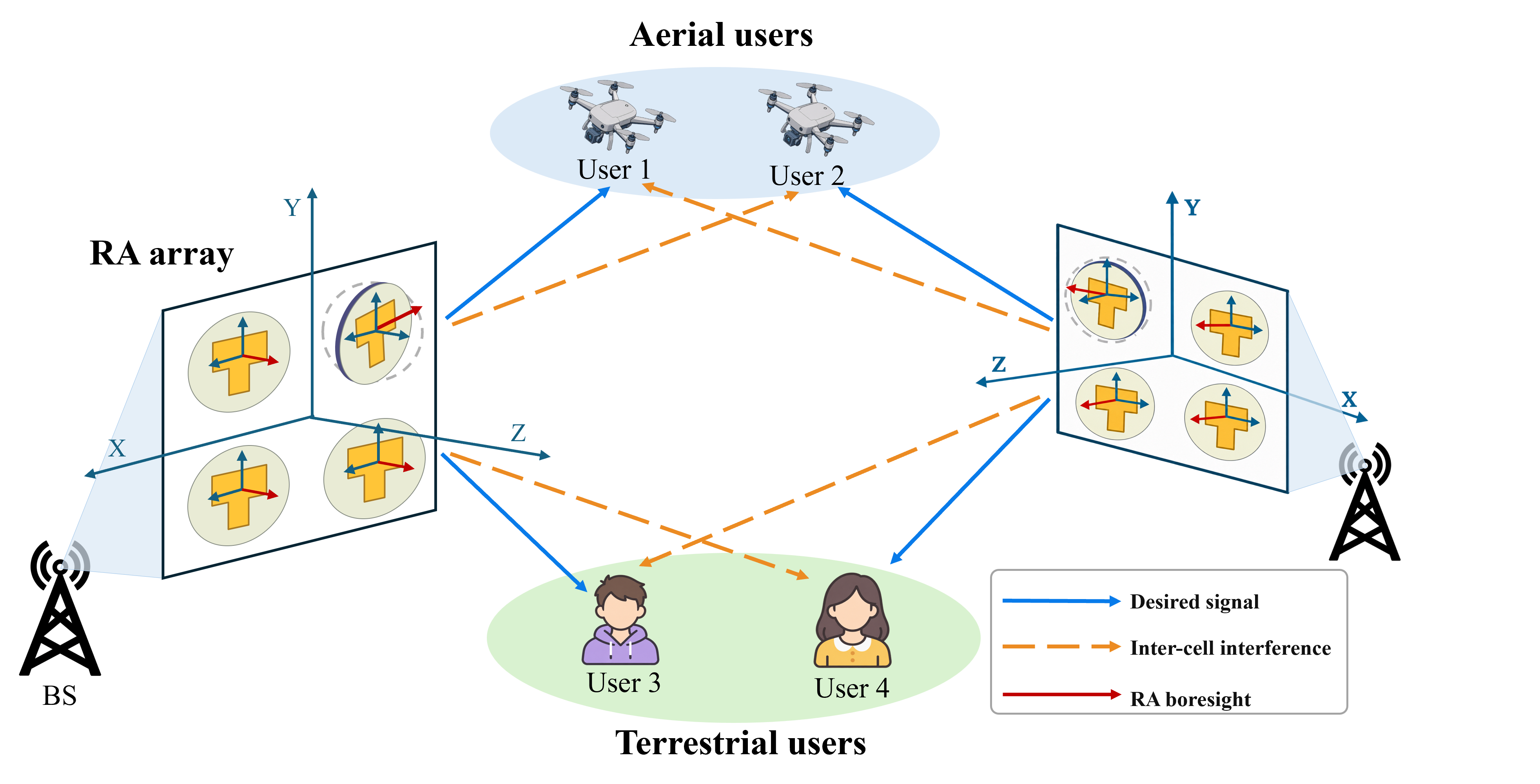
As illustrated in Fig. 1, we consider an RA-enabled LAE network, which consists of BSs and users, denoted by the sets and , respectively. In this network, the users include both conventional terrestrial users and low-altitude aerial users. Each BS is equipped with RAs to serve both types of users. Without loss of generality, we assume that each user is equipped with a single isotropic antenna and each BS employs a uniform planar array (UPA) with antennas, where and denote the number of antennas along the - and - axes, respectively.
II-A RA Configuration
To support 3D coverage for LAE networks, we deploy RAs at multiple BSs where each RA has an independently adjustable boresight direction. Specifically, the boresight direction of the -th RA at BS is characterized by a pointing vector
| (1) |
where , , and denote the components along the -, -, and -axes, respectively. Let denote the zenith angle (i.e. the angle between the boresight direction and the positive -axis), and let denote the azimuth angle (i.e. the angle between the projection onto the - plane and the positive -axis). The pointing vector can then be expressed as
| (2) |
To account for the limited rotation range, the zenith angle of each RA is subject to
| (3) |
where denotes the maximum zenith angle. Accordingly, the matrix of the RA orientations at BS is given by . The collection of orientation matrices across all BSs is then denoted by
| (4) |
To highlight the advantage of adjusting RA orientations, we adopt a directional radiation pattern based on [20], given by
| (5) |
where denotes the angular misalignment between the boresight direction and the signal propagation direction, is the antenna directivity factor, and is the maximum directional gain.
II-B Channel Model
In this subsection, we present a channel model for the considered RA-enabled LAE networks.
Let denote the center position of the UPA at BS in the global Cartesian coordinates, and let denote the position of user . Each RA is indexed by , where and . For notational convenience, the two-dimensional indices of RAs can be presented by a single index:
| (6) |
where is defined as . The position of the -th RA at BS is then given by
| (7) |
where is the wavelength. The distance between the -th RA at BS and user is denoted as , and the corresponding unit propagation direction is . Based on the RA radiation pattern in Eq. (5), the directional antenna gain of the -th antenna at BS toward user is expressed as
| (8) |
Thus, based on the Friis transmission model [28], the channel between the -th antenna at BS and user is given by
| (9) |
where denotes the free space channel power gain at the reference distance, denotes the unit direction vector from BS to user , while represents the relative position of the -th RA with respect to the center position of BS . Thus, the channel vector from BS to user can be written as
| (10) |
II-C Signal Model
In this subsection, we develop a signal model combined with user association where each user is associated with only one BS. Specifically, let denote the user association variable for all and , where if and only if user is associated with BS . Since each user is served by only one BS, the association variables satisfy
| (11) |
We denote the set of all association variables as .
For the transmission, let denote the transmit data intended for user from BS satisfying , and let denote the corresponding transmit beamforming vector. Then the signal from BS can be expressed as
| (12) |
It is worth noting that is set to zero when user is not associated with BS , i.e., if . Accordingly, the received signal at user is given by
| (13) |
where represents the additive white Gaussian noise (AWGN) at user . When user is served by BS , its corresponding signal-to-interference-plus-noise ratio (SINR) is given by
| (14) |
Then the achievable rate is expressed as
| (15) |
III Problem Formulation
Based on the above system model, the user association affects the optimal RA orientations, since different serving BSs result in different propagation directions. However, it is not straightforward to determine the RA orientations jointly with the user association. Therefore, we consider a network sum-rate maximization problem which jointly optimizes user association , transmit beamforming and the RA orientations . The resulting optimization problem is formulated as
| (16a) | ||||
| s.t. | (16b) | |||
| (16c) | ||||
| (16d) | ||||
| (16e) | ||||
| (16f) | ||||
The objective of problem P1 is to maximize the network sum-rate, defined as the sum of weighted by their corresponding association variables. Constraint (16b) imposes an individual transmit power budget at each BS, where denotes the maximum transmit power of BS . Moreover, constraints (16c) and (16d) jointly define the feasible set for user association. Specifically, the binary variable indicates that user is associated with BS , and otherwise, while constraint (16d) ensures that each user is served by only one BS. Constraint (16e) ensures that the orientation vector of each RA is normalized. Constraint (16f) limits the maximum rotation angle of each RA boresight from the initial direction . Given that , this is equivalent to .
It is worth noting that problem P1 does not explicitly impose the coupling constraint when because omitting this constraint does not affect the optimal objective value. To see this, suppose that there exists an optimal solution satisfying but . Setting does not affect the corresponding sum-rate, since . Meanwhile, setting reduces the transmit power consumption at BS and cannot increase the interference experienced by any served user. Therefore, the system sum-rate cannot decrease. Hence, there always exists an optimal solution satisfying whenever for all and .
IV Proposed Solution
Problem P1 is challenging to solve directly, as it requires the joint optimization of the user association, transmit beamforming, and RA orientations. Moreover, the effective channels depend on the RA orientations, making the problem non-convex.
To address these challenges, we first reformulate the sum-rate objective using the WMMSE equivalence by introducing the auxiliary variables and . Then, we develop an AO algorithm that sequentially updates the auxiliary variables and , the user association , the transmit beamforming , and the RA orientations , while keeping the remaining variables fixed.
IV-A Problem Reformulation
In this subsection, we reformulate the non-convex sum-rate objective into an equivalent WMMSE form to facilitate the joint optimization [29]. Specifically, we introduce the auxiliary variable , which denotes the scalar receive equalizer associated with the link from BS to user . The estimate of is then given by . The corresponding mean square error (MSE) is
| (17) |
Substituting the received signal given by Eq. (13) into Eq. (17) yields
| (18) |
where denotes the total received power at user .
For fixed transmit beamforming , minimizing with respect to leads to the minimum mean square error (MMSE) equalizer
| (19) |
By substituting Eq. (19) into Eq. (18), the corresponding MMSE is then obtained as
| (20) |
Therefore, the achievable rate from BS to user can be equivalently expressed as . By introducing a positive weight , the following identity holds for any
| (21) |
Solving the maximization problem in Eq. (21) with respect to yields the optimal weight
| (22) |
By combining Eq. (20) with Eq. (21), the achievable rate from BS to user can be equivalently expressed as
| (23) |
Consequently, the original sum-rate maximization problem P1 can be equivalently reformulated as the following problem
| (24) | ||||
where and . For any fixed , , and , the optimal variables and are given by Eq. (19) and Eq. (22), respectively.
IV-B Optimization for User Association
In this subsection, we optimize the user association with fixed , , , and . Since the transmit power constraint (16b) and the RA orientation constraints (16e)–(16f) are independent of , they can be omitted from the user association subproblem. The resulting subproblem is formulated as
| (25) | ||||
Problem P3 is non-convex because of the binary association constraint (16c). To facilitate this optimization, we relax from the binary set to . Together with constraint (16d), the relaxed feasible set is defined as
| (26) |
where for all .
Accordingly, the problem P3 can be formulated as
| (27a) | ||||
| (27b) | ||||
where .
It is obvious that problem P3.1 has an optimal solution where user assigns its entire association weight to a single BS . Hence, there exists an optimal solution in which is binary for all and . Consequently, the relaxed problems P3.1 is equivalent to problem P3 and attains the same optimal objective value. However, solving problem P3.1 directly to optimality may yield a low-quality solution because the AO algorithm is highly sensitive to the initial point. To solve it, we therefore perform a projected gradient ascent step mentioned in [30] at each iteration as
| (28) |
where is the stepsize and denotes the Euclidean projection onto the set . Details of the projection procedure are provided in Appendix A.
After the AO iterations, a binary recovery step is performed to enforce the constraint (16c). Specifically, for each user , we select , and then recover the binary association as
| (29) |
IV-C Optimization for Transmit Beamforming
In this subsection, we optimize the transmit beamforming with fixed , , , and . Since the terms and the positive factor are independent of , problem P2 can be reduced to the following subproblem
| (30) | ||||
Substituting Eq. (18) into the objective function in Eq. (30) and omitting the terms independent of , problem P4 can be decomposed into independent subproblems. For BS , the corresponding subproblem is given by
| (31) | ||||
where is denoted as .
Let denote the Lagrange multiplier associated with the power constraint (16b). Then, the Lagrangian of problem P4.1 is given by
| (32) | ||||
Taking the Wirtinger derivative with respect to gives
| (33) |
According to the Karush–Kuhn–Tucker (KKT) stationarity condition, the optimal transmit beamforming vector is given by
| (34) |
The Lagrange multiplier is determined independently for each BS via bisection to satisfy the power constraint (16b).
IV-D Optimization for the Orientations of RAs
In this subsection, we optimize the RA orientations with , , , and fixed. The resulting subproblem is formulated as
| (35) | ||||
Here, denotes the objective function of problem P2 in Eq. (24), and is the collection of for all and . The feasible set defined by constraints (16e) and (16f) is
| (36) |
Problem P5 is challenging due to the coupling between the RA orientations and the effective channels, together with the non-convex feasible set . To address these difficulties, we adopt a Frank-Wolfe method to optimize the RA orientations [31, 24]. At each iteration, the procedure constructs an approximation of problem P5 at the current feasible orientations, then solves the resulting subproblem, and updates the RA orientations using a stepsize selected by Armijo backtracking.
Specifically, at iteration , we first compute the gradient of with respect to the RA orientation , given by
| (37) |
which is detailed in Appendix B. However, since constraint (16e) restricts to a unit sphere, we have to project the gradient onto the tangent space as
| (38) |
where is the corresponding orthogonal projection matrix.
To simplify the optimization of the nonlinear objective , we then use the projected gradients to approximate around the current orientations as
Replacing the objective function of problem P5 with this approximation results in the following subproblem
| (39) | ||||
After omitting the term independent of , problem P5.1 can be decomposed into the following subproblem for each
| (40) | ||||
We denote as an optimal solution for problem P5.2, given in Eq. (41), where is any unit vector orthogonal to .
|
|
(41) |
Consequently, the Frank-Wolfe search directions are given by
| (42) |
Then, the antenna orientations can be updated as
| (43) |
where is the stepsize, selected by the following Armijo condition:
| (44) |
The parameter in Eq. (44) is an Armijo constant, while denotes an aggregate improvement of the objective in problem P5.2 for all and . Specifically, it is defined as
| (45) | ||||
Given that consistently holds, . Meanwhile, it is proved that there always exists a stepsize satisfying condition (44) at each iteration [24]. Therefore, , guaranteeing the objective sequence is monotonically non-decreasing. The procedure for optimizing the RA orientations is summarized in Algorithm 1.
In summary, the overall algorithm to solve the problem P1 is summarized in Algorithm 2.
IV-E Convergence and Complexity Analysis
1) Convergence Analysis: Let denote the objective function of problem P1. For updating the user association , Appendix A establishes that the updating procedure does not decrease the objective value, as shown in Eq. (62). In the subsequent beamforming update, is optimized with and fixed. Since the subproblem P4 is convex, Eq. (34) provides an optimal solution. Because remains feasible with constraints unchanged, the update cannot increase the objective of problem P4 and, equivalently, cannot decrease the objective . We then update the RA orientations using the Frank-Wolfe method. According to the Armijo condition in Eq.(44), the objective value of the subproblem P5 is monotonically non-decreasing. Consequently, we have . Therefore, the sequence is monotonically non-decreasing.
Moreover, the bound , together with the transmit power constraint (13b), ensures that the objective value is bounded above. Hence, the monotonically non-decreasing sequence is convergent.
2) Computational Complexity: We analyze the computational complexity in terms of the AO iterations. For the updates of and , the optimal solutions are given by Eq. (19) and Eq. (22), respectively. The computational cost is dominated by evaluating for each user , whose complexity is . Aggregating this cost over all users yields . For the update of , the main computational complexity comes from the projection in Eq. (28). As detailed in Appendix A, the projection sorts the entries of the vector for each user , which has a complexity of . Thus, updating for all users has a complexity of . For the update of in Eq. (34), the complexity of constructing for all is . Inverting each matrix has a complexity of , totaling for all BSs. Since the bisection search of generally takes only a few iterations, its complexity is omitted. Consequently, the overall complexity of updating is . For the update of , the complexity is dominated by gradient evaluation in Eq. (69). Each gradient evaluation requires a complexity of , leading to an overall complexity of . Let denote the number of AO iterations and denote the number of Frank-Wolfe iterations per AO step. The total computational complexity is then given by
| (46) | ||||
V Low-Complexity Joint Optimization Algorithms
However, optimizing the RA orientations requires iterative updates, and the associated computational complexity increases with the number of RAs. In this section, we develop two low-complexity algorithms that simplify the optimization of RA orientations while leaving the updates of the remaining variables unchanged.
V-A Discrete Candidate-Scanning Algorithm
In this subsection, we develop a discrete candidate-scanning-based algorithm that sequentially updates each RA orientation by selecting the direction from a finite candidate set that maximizes the objective.
As indicated in Eq. (8), the directional antenna gain of an RA is maximized when the boresight is aligned with the user direction. Therefore, the user directions provide a natural basis for constructing a finite set of candidate orientations. However, a user direction may violate the rotation constraint (16f). To ensure feasibility, we define to project any user direction onto the feasible region . Then the candidate set for the -th RA at BS is constructed as
| (47) |
The current orientation is included in so that the objective value cannot decrease. With , , , and fixed, the subproblem remains as formulated in problem P5. Rather than evaluating the orientation gradient, the proposed method updates by selecting a candidate orientation according to
| (48) |
Since , the update in Eq. (48) satisfies
| (49) |
The complete procedure is summarized in Algorithm 3.
V-B Antenna Block-Based Algorithm
In this subsection, we develop a low-complexity antenna-block-based algorithm that reduces the number of orientation variables by partitioning the RAs at each BS into multiple blocks. All RAs within each block share a common boresight direction.
Let denote the block index set for BS . We partition the RA index set into blocks, satisfying
| (50) |
where denotes the set of RAs assigned to block . For each and , let denote the shared boresight direction of block at BS . Thus, every RA in satisfies
| (51) |
Accordingly, the subproblem can be written as
| (52a) | ||||
| (52b) | ||||
where . Since all RAs within block share the same boresight direction, we optimize only the shared variable rather than the individual orientation of every RA in the block. Problem P6 has the same constraint structure as problem P5. Therefore, is optimized following the same procedure described in Algorithm 1.
VI Simulation Results
In this section, we evaluate the performance of the proposed algorithm. Unless otherwise specified, the simulation parameters are set as follows. As illustrated in Fig. 2, six BSs are deployed in a regular hexagonal layout, each equipped with a UPA oriented toward the network center. The distance between adjacent BSs and the BS height are set to m and m, respectively. The carrier wavelength is set to m and the inter-element spacing is set to . The network serves users, including eight terrestrial users at a height of m and eight aerial users whose heights are uniformly distributed over m. The transmit power per BS and the receiver noise power are set to dBm and dBm, respectively. The RA directivity factor is set to and the maximum rotation angle is set to . The key simulation parameters are summarized in Table I.

| Parameter | Value | Parameter | Value |
|---|---|---|---|
| Number of BSs, | Number of users, | ||
| Distance between adjacent BSs | m | BS height | m |
| Number of terrestrial users | Terrestrial user height | m | |
| Number of aerial users | Aerial user height | m | |
| UPA size, | Wavelength, | m | |
| Inter-element spacing, | Transmit power per BS, | dBm | |
| Receiver noise power, | dBm | Directivity factor, | |
| Maximum rotation angle, |
VI-A Performance of the Proposed Algorithm
In this subsection, we evaluate the performance gains of the proposed joint design in Algorithm 2 compared with five benchmark schemes, which are defined as follows:
- •
Baseline 1 (fixed antenna orientations): User association is optimized, and transmit beamforming is optimized using WMMSE, while the RA orientations are fixed.
- •
Baseline 2 (nearest BS association): Each user is associated with its nearest BS, whereas the RA orientations are optimized and transmit beamforming is optimized using WMMSE.
- •
Baseline 3 (nearest BS association and fixed antenna orientations): Each user is associated with its nearest BS, and the RA orientations are fixed. In this scheme, only transmit beamforming is optimized using WMMSE.
- •
Baseline 4 (maximum ratio transmission, MRT): User association and the RA orientations are optimized, while the MRT algorithm is used for beamforming.
- •
Baseline 5 (zero forcing, ZF): User association and the RA orientations are optimized, while the ZF algorithm is used for beamforming.

Fig. 3 illustrates the convergence behavior of the proposed algorithm alongside Baselines 1–3. It can be observed that all four curves increase monotonically over the iterations. At convergence, the proposed algorithm achieves the highest sum-rate compared with the three benchmarks, demonstrating its performance superiority. Moreover, Baseline 2 achieves a higher sum-rate than Baseline 1, indicating that the gain from optimizing the RA orientations outweighs that from optimizing user association.

Fig. 4 depicts the sum-rate versus transmit power per BS. All schemes exhibit a monotonic increase with transmit power, and the proposed algorithm consistently attains the highest sum-rate. At the lowest transmit power of dBm, Baseline 4 with MRT performs nearly as well as the proposed algorithm with WMMSE and slightly outperforms Baseline 5 with ZF. This observation is consistent with a noise-limited scenario, in which enhancing the desired signal is more important than suppressing multi-user interference. As power increases, however, Baseline 5 surpasses Baseline 4 and thereafter remains the closest benchmark to the proposed algorithm, owing to the interference suppression capability of ZF. Moreover, the gap between the proposed algorithm and the fixed orientation scheme Baseline 1 widens as transmit power increases, indicating that orientation optimization becomes increasingly beneficial in the interference-limited scenario, where RA can reshape the channel conditions to strengthen desired links and mitigate inter-user interference.

Fig. 5 examines the impact of the maximum rotation angle on the system sum-rate. As expected, Baselines 1 and 3 remain invariant with respect to due to the fixed RA orientations. In contrast, the sum-rates of the remaining schemes increase monotonically with and gradually approach plateaus at approximately rad, suggesting that the antennas can fully cover the user distribution range. Among the schemes with optimized RA orientations, the proposed algorithm achieves the highest sum-rate, followed by Baselines 5, 2, and 4. At , the feasible orientation set is limited to the reference directions. Accordingly, the proposed algorithm coincides with Baseline 1, while Baseline 2 coincides with Baseline 3. The gap between these two pairs reflects the performance gain of optimized user association.

Fig. 6 illustrates the effect of the antenna directivity factor on the sum-rate. At , the antenna gain in Eq. (5) becomes constant and independent of angular misalignment. Hence, optimizing the RA orientations yields no additional benefit. In this case, the proposed algorithm coincides with Baseline 1, and Baseline 2 coincides with Baseline 3. As increases, the sum-rates achieved by the proposed algorithm and Baselines 2, 4, and 5 all increase monotonically, because higher directivity enhances the benefit of steering main lobes toward intended users while suppressing interference. In contrast, the fixed orientation schemes exhibit a slight improvement at , after which the performance declines steadily. The reason is that at low directivity, the increase in outweighs the gain loss caused by boresight misalignment, thereby improving the effective channel gains. However, as increases, the narrowing beam pattern aggravates the misalignment loss, which in turn results in the decline.

Fig. 7 evaluates the effect of the UPA dimension , where each BS employs an array comprising RAs. The sum-rates of all schemes increase monotonically with . This improvement is attributed to the larger array gain and additional spatial degrees of freedom, which facilitate more effective multi-user beamforming. Furthermore, it is observed that the proposed algorithm consistently achieves the highest sum-rate across all considered array configurations. Meanwhile, its performance gap relative to Baseline 2 narrows as increases. This trend indicates that the benefit of optimizing user association becomes less significant for larger arrays.
VI-B Performance of the Low-Complexity Algorithms
In this subsection, we evaluate the low-complexity algorithms developed in Section V against the proposed algorithm in Algorithm 2. All schemes share the same updates for , , , and , and differ only in the update of . The following low-complexity schemes are considered:
- •
Antenna block-based: The RAs are partitioned into blocks. All RAs within a block share one boresight direction, which is optimized using the Frank-Wolfe update.
- •
Discrete candidate-scanning: Each RA retains an independent boresight, but its orientation is selected from a finite candidate set in Eq. (47).
- •
Combined scheme: Each block shares one boresight direction, which is updated using discrete candidate scanning.

Fig. 8 illustrates the effect of antenna block size on the sum-rate for a UPA. In this comparison, the curve corresponds to the proposed algorithm in Algorithm 2, where each RA boresight is treated as an independent optimization variable. The scheme divides the UPA into four blocks, whereas the scheme assigns a single common orientation to the entire array. The sum-rates of all three schemes increase monotonically with transmit power, and the scheme consistently achieves the highest sum-rate among them. In particular, the scheme achieves a sum-rate closer to that of the scheme, while the scheme experiences a larger performance degradation. These results indicate that performance loss increases with block size.

Fig. 9 compares the three low-complexity schemes with the proposed algorithm under the UPA configuration, in which the antenna block-based scheme uses blocks. The sum-rates of all four schemes increase monotonically with transmit power, and the proposed algorithm consistently achieves the highest sum-rate. The antenna block-based scheme incurs the smallest performance loss relative to the proposed algorithm, because sharing orientations within small blocks retains substantial flexibility in antenna orientation while reducing the number of optimization variables. In contrast, the discrete candidate-scanning scheme suffers a larger degradation, as restricting each boresight to a finite set of user directions sacrifices the flexibility of continuous adjustment.
VII Conclusion
In this paper, we have investigated an RA-enabled LAE network in which multiple BSs serve both terrestrial and aerial users. We have formulated a sum-rate maximization problem that jointly optimizes user association, transmit beamforming, and the RA orientations. To address the resulting non-convex problem, we have developed an AO algorithm with projected gradient ascent, the WMMSE algorithm, and the Frank-Wolfe algorithm. We have further developed two low-complexity algorithms that reduce the computational cost of orientation optimization. Simulation results have confirmed that the proposed AO algorithm achieves the highest sum-rate among the evaluated schemes across the examined settings, while the two low-complexity algorithms retain most of the achievable gain with lower orientation update complexity.
Appendix A Derivation of the User-Association Projection
This appendix derives the Euclidean projection presented in Eq. (28). For notational convenience, we denote as . Then the projection of onto is equivalently written as
| (53a) | ||||
| (53b) | ||||
| (53c) | ||||
The problem P7 is strictly convex and has a unique globally optimal solution. We denote as the Lagrange multiplier vector associated with constraint (53b), and denote as the Lagrange multiplier associated with constraint (53c), respectively. Then, the Lagrangian is
| (54) | ||||
The corresponding KKT conditions are
| (55a) | ||||
| (55b) | ||||
| (55c) | ||||
| (55d) | ||||
| (55e) | ||||
From Eq. (55a), the -th component satisfies
| (56) |
If , Eq. (55e) requires , and hence . Otherwise, . Combining these two cases gives the following closed-form expression for :
| (57) |
Substitution Eq. (57) into Eq. (55c) yields
| (58) |
Let denote the entries of sorted in non-increasing order. The Lagrange multiplier is then given by
| (59) |
where denotes the number of active components of and is computed by
| (60) | ||||
According to the first-order optimality condition, the optimal obtained from Eq. (57) satisfies
| (61) |
Setting and replacing with yield
| (62) |
which means the association update does not decrease the objective.
Appendix B Derivation of the RA Orientation Gradient
With , , , and fixed in problem P5, only the MSE term depends on . Applying the chain rule to the WMMSE objective in Eq. (24) gives
| (63) |
Similarly, is given by
| (64) |
where denotes the total received power at user . Only channels from BS depend on . Therefore, the received power derivative is
| (65) |
Similarly,
| (66) |
For notational convenience, let denote the gradient of the effective channel coefficient with respect to the orientation . By Eq. (10), affects only the -th entry of . Therefore,
| (67) |
Differentiating Eq. (9) with respect to yields
| (68) | ||||
We adopt the convention that whenever , which selects the zero Clarke subgradient at the visibility boundary [24]. Substituting Eqs. (65)–(67) into Eq. (64), and then substituting the result into (63), yields
| (69) | ||||
References
- [1] (2023) 6G non-terrestrial networks enabled low-altitude economy: opportunities and challenges. arXiv preprint arXiv:2311.09047. Cited by: §I.
- [2] (2025) Toward realization of low-altitude economy networks: core architecture, integrated technologies, and future directions. IEEE Trans. Cognit. Commun. Netw. 11 (5), pp. 2788–2820. External Links: Document Cited by: §I.
- [3] (2026) Ubiquitous UAV communication enabled low-altitude economy: applications, techniques, and 3GPP’s efforts. IEEE Netw. 40 (1), pp. 115–122. External Links: Document Cited by: §I.
- [4] (2026) Satellite-assisted low-altitude economy networking: concepts, applications, and opportunities. IEEE Wireless Commun. 33 (3), pp. 177–186. External Links: Document Cited by: §I.
- [5] (2017) Coexistence of terrestrial and aerial users in cellular networks. In Proc. IEEE Globecom Workshops (GC Wkshps), pp. 1–6. Cited by: §I, §I.
- [6] (2023) Dedicating cellular infrastructure for aerial users: advantages and potential impact on ground users. IEEE Trans. Wireless Commun. 22 (4), pp. 2523–2535. External Links: Document Cited by: §I, §I.
- [7] (2021) Ensuring reliable connectivity to cellular-connected UAVs with up-tilted antennas and interference coordination. ITU J. Future and Evolving Technol. 2 (2), pp. 165–185. External Links: Document Cited by: §I, §I.
- [8] (2026) FMCW-enabled integrated sensing, identification, and backscatter communication for low-altitude economy. IEEE Trans. Wireless Commun. 25 (), pp. 10953–10967. External Links: Document Cited by: §I.
- [9] (2025) Integrated sensing and communication for low altitude economy: opportunities and challenges. IEEE Commun. Mag. 63 (12), pp. 72–78. External Links: Document Cited by: §I.
- [10] (2026) Integrated sensing, identification, and backscatter communications: a tensor-based multi-antenna framework. IEEE Trans. Commun. (), pp. 1–1. External Links: Document Cited by: §I.
- [11] (2022) A survey on the convergence of edge computing and AI for UAVs: opportunities and challenges. IEEE Internet Things J. 9 (17), pp. 15435–15459. External Links: Document Cited by: §I.
- [12] (2020) Joint task offloading and resource allocation in UAV-enabled mobile edge computing. IEEE Internet Things J. 7 (4), pp. 3147–3159. External Links: Document Cited by: §I.
- [13] (2020) A survey on cellular-connected UAVs: design challenges, enabling 5G/B5G innovations, and experimental advancements. Comput. Netw. 182, pp. 107451. External Links: ISSN 1389-1286, Document Cited by: §I.
- [14] (2019) Survey on UAV cellular communications: practical aspects, standardization advancements, regulation, and security challenges. IEEE Commun. Surveys & Tut. 21 (4), pp. 3417–3442. External Links: Document Cited by: §I.
- [15] (2019) Cellular-connected UAV: potential, challenges, and promising technologies. IEEE Wireless Commun. 26 (1), pp. 120–127. External Links: Document Cited by: §I.
- [16] (2019) Optimal base station antenna downtilt in downlink cellular networks. IEEE Trans. Wireless Commun. 18 (3), pp. 1779–1791. External Links: Document Cited by: §I.
- [17] (2018) Supporting UAV cellular communications through massive MIMO. In Proc. IEEE Int. Conf. Commun. Workshops (ICC Wkshps), Vol. , pp. 1–6. External Links: Document Cited by: §I.
- [18] (2026) Rotatable antenna-empowered wireless networks: a tutorial. arXiv preprint arXiv:2603.25559. Cited by: §I.
- [19] (2026) Rotatable antenna enabled wireless communication and sensing: opportunities and challenges. IEEE Wireless Commun. 33 (3), pp. 134–141. External Links: Document Cited by: §I.
- [20] (2026) Rotatable antenna-enabled wireless communication: modeling and optimization. IEEE Trans. Commun. 74, pp. 6825–6842. External Links: Document Cited by: §I, §II-A.
- [21] (2025) Efficient channel estimation for rotatable antenna-enabled wireless communication. IEEE Wireless Commun. Lett. 14 (11), pp. 3719–3723. External Links: Document Cited by: §I.
- [22] (2026) Polarization-aware reconfigurable antenna aided wireless communications. IEEE Trans. Wireless Commun. 25 (), pp. 22386–22401. External Links: Document Cited by: §I.
- [23] (2026) Polarization-aware rotatable antennas for RIS-empowered symbiotic radios. arXiv preprint arXiv:2609.03484. Cited by: §I.
- [24] (2026) Rotatable antenna enabled spectrum sharing: joint antenna orientation and beamforming design. IEEE Trans. Wireless Commun. 25, pp. 15660–15674. External Links: Document Cited by: Appendix B, §I, §IV-D, §IV-D.
- [25] (2026) Rotatable antenna system empowered low-altitude economy: opportunities and challenges. IEEE Wireless Commun. 33 (1), pp. 116–123. External Links: Document Cited by: §I.
- [26] (2019) Cellular-connected UAV: uplink association, power control and interference coordination. IEEE Trans. Wireless Commun. 18 (11), pp. 5380–5393. Cited by: §I.
- [27] (2021) Joint beamforming, user association, and height control for cellular-enabled UAV communications. IEEE Trans. Commun. 69 (6), pp. 3598–3613. Cited by: §I.
- [28] (2016) Antenna theory: analysis and design. Hoboken, NJ, USA: Wiley. Cited by: §II-B.
- [29] (2011) An iteratively weighted MMSE approach to distributed sum-utility maximization for a MIMO interfering broadcast channel. IEEE Trans. Signal Process. 59 (9), pp. 4331–4340. External Links: Document Cited by: §IV-A.
- [30] (2014) Optimal joint base station assignment and beamforming for heterogeneous networks. IEEE Trans. Signal Process. 62 (8), pp. 1950–1961. External Links: Document Cited by: §IV-B.
- [31] (2013) Revisiting Frank-Wolfe: projection-free sparse convex optimization. In Proc. Int. Conf. Machine Learning (ICML), Vol. 28, pp. 427–435. Cited by: §IV-D.