Diffusion Subgoal Planning for Long-Horizon Offline Goal-Conditioned Reinforcement Learning

Hengrui Zhang Yuhu Cheng C. L. Philip Chen Xuesong Wang ^†^†thanks: Corresponding author. Email: {hengruizhang, chengyuhu, wangxuesong}@cumt.edu.cn Affiliation: School of Information and Control Engineering, China University of Mining and Technology Affiliation: School of Computer Science and Engineering, South China University of Technology Email: philip.chen@ieee.org

Abstract

Offline goal-conditioned reinforcement learning (GCRL) learns goal-directed policies from reward-free data, but in long-horizon tasks, goal-conditioned value functions often provide unstable guidance due to sparse rewards and discounting. Hierarchical methods partially mitigate this issue via subgoal decomposition; however, high-level decision-making still relies on noise-sensitive value estimates, leading to unstable behavior in complex environments. We address this limitation by proposing Diffusion Subgoal Planning (DSP), a diffusion-based framework for high-level subgoal generation. DSP casts high-level planning as guided generative inference over goal-conditioned subgoals and learns both conditional and unconditional flows, enabling classifier-free guidance to introduce a goal-directed bias at inference time. By removing explicit value-based guidance from high-level planning, DSP generates reachable and goal-directed subgoals through a generative model while retaining hierarchical execution. Experiments on offline GCRL benchmarks demonstrate that DSP outperforms prior methods on a range of navigation and manipulation tasks, with particularly strong performance in maze environments that require multi-step subgoal planning.

Project page: https://henry0132.github.io/DSP

Repository: https://github.com/Henry0132/DSP

1 Introduction

Goal-conditioned reinforcement learning (GCRL) formulates decision-making problems in terms of desired outcomes, reducing the need to manually design reward functions in high-dimensional spaces and enabling task generalization [14, 36, 16]. Offline GCRL [45, 53] further extends this setting to learning solely from reward-free trajectories, resembling self-supervised learning from past experience. However, without explicit rewards, desired goals are often temporally distant, and value function estimation can suffer from limited data coverage and accumulated errors [47, 15, 29], resulting in noisy and unreliable learning signals in long-horizon tasks.

Hierarchical Implicit Q-Learning (HIQL) [47] addresses long-horizon challenges by introducing a two-level policy, where a high-level policy proposes intermediate subgoals and a low-level policy executes actions conditioned on them. While this hierarchy improves stability over flat policies, large-scale offline GCRL evaluations show that in tasks involving complex navigation, spatial search, or high-dimensional manipulation, HIQL can struggle to obtain reliable guidance from noisy value functions, leading to degraded performance [45, 1, 44]. Subsequent analyses attribute these failures in part to imprecise value guidance and the resulting errors in high-level planning [46, 1]. Since hierarchical performance depends critically on subgoal quality, several methods seek to improve value estimation itself, such as Pi-HIQL [15], which enforces geometric structure via Eikonal regularization, and OTA [1], which promotes hierarchical consistency through option-aware mechanisms.

However, these approaches share a common assumption that high-level planning should be driven by value function estimates. When subgoals are selected through noisy values, long-horizon planning can remain unstable. This naturally raises a central question:

Can hierarchical planning be retained without value-based high-level guidance?

Diffusion models [19, 56] provide a promising alternative to value-based planning by generating reachable intermediate states that reflect the structure of the offline data distribution [24, 2]. Moreover, goal-directed preferences can be incorporated into the sampling process via guidance mechanisms such as classifier-free guidance (CFG) [20], enabling controllable subgoal generation without explicit high-level value estimation.

Motivated by these properties, we propose Diffusion Subgoal Planning (DSP), a diffusion-based framework for high-level subgoal generation in offline GCRL. DSP formulates high-level planning as guided generative inference over goal-conditioned subgoals, enabling high-level decision-making without explicit value-based guidance while preserving the benefits of hierarchical execution. Concretely, DSP learns both conditional and unconditional velocity fields, and uses classifier-free guidance at inference time to bias subgoal generation toward the desired goal. This guidance mechanism further admits an implicit advantage-weighted interpretation at the subgoal level. Experiments on offline GCRL benchmarks demonstrate that DSP outperforms prior methods on a range of navigation and manipulation tasks, with particularly strong gains in long-horizon maze environments that require multi-step subgoal planning.

2 Related Works

Offline GCRL. Offline goal-conditioned reinforcement learning aims to learn a universal policy that reaches arbitrary target states from arbitrary initial states using a fixed dataset [50, 14, 43, 45]. Most approaches treat goals as future states and adopt self-supervised training schemes, including hindsight relabeling [3, 11], state occupancy matching [53, 10], and related goal relabeling methods [42, 57]. Recent work further incorporates hierarchical structures to decompose complex tasks into multi-step plans via recursive subgoal inference [47, 15, 1, 25, 32]. Despite differences in formulation, these methods share a common assumption that high-level subgoals are optimized using learning signals derived from goal-conditioned value functions, making noisy value estimates a central bottleneck for reliable long-horizon planning in offline settings.

Hierarchical RL. Hierarchical reinforcement learning introduces decision-making at multiple temporal scales to address long-horizon planning and exploration [17, 5, 13]. Early approaches rely on graph-based subgoal planning [65, 27], while later methods generate intermediate waypoints using temporal distance [37], latent abstractions [9, 13], or value-based criteria [1, 52]. Although these approaches aim to simplify planning by defining reachable high-level subgoals, graph-based methods are often computationally expensive and difficult to scale [51, 31, 4], while waypoint prediction methods that depend on value functions or distance estimates are highly sensitive to estimation accuracy, particularly under sparse data coverage [10]. As a result, existing hierarchical RL methods can remain sensitive to value-function noise, particularly in offline settings [45].

Diffusion Policies for RL. Diffusion models have been adopted in reinforcement learning as expressive generative models [19, 54, 55, 56, 35, 38], with applications to action generation [60, 39, 7, 18], trajectory modeling [2, 34], and goal-conditioned or planning-oriented generation [23, 26, 63]. Recent methods further use guidance or flow matching to improve action-level policy learning and controllability [12, 48]. Other works explore hierarchical diffusion-based planning or subgoal generation [33, 6, 64], where diffusion models are typically used as trajectory or milestone planners [22, 21], often combined with MPC, return guidance, or multi-step planning procedures. In contrast, DSP uses guided generation as a high-level subgoal decision mechanism in hierarchical offline GCRL, replacing explicit value-based subgoal selection while retaining a separately trained low-level executor.

3 Preliminaries

Problem Setting. Offline GCRL is formulated as a finite-horizon discounted Markov decision process $\mathcal{M}=(\mathcal{S},\mathcal{A},\mathcal{G},\mathcal{P},r,\mathcal{P}_{g},d_{0},\gamma)$ , where $\mathcal{S}$ , $\mathcal{A}$ , and $\mathcal{G}$ denote the state, action, and goal spaces, respectively. The transition dynamics are given by $\mathcal{P}(s^{\prime}\mid s,a)$ , and the reward function is $r(s,g)$ . The initial state distribution $d_{0}$ and goal distribution $\mathcal{P}_{g}$ specify how episodes are initialized. The discount factor is $\gamma\in[0,1)$ . Following standard practice, we assume $\mathcal{G}=\mathcal{S}$ . At the beginning of each episode, a goal $g\sim\mathcal{P}_{g}$ is sampled, and the agent aims to reach $g$ by maximizing the expected discounted return $J(\pi)=\mathbb{E}_{\tau\sim\pi(\cdot\mid g)}\left[\sum_{t=0}^{T}\gamma^{t}r(s_{t},g)\right]$ , where $\tau=(s_{0},a_{0},s_{1},a_{1},\ldots,s_{T})$ is a trajectory induced by a goal-conditioned policy $\pi(a\mid s,g)$ . The corresponding goal-conditioned value function is $V^{\pi}(s,g)=\mathbb{E}_{\tau\sim\pi(\cdot\mid g)}\left[\sum_{t=0}^{T}\gamma^{t}r(s_{t},g)\;\middle|\;s_{0}=s\right].$ In the offline setting, the policy is learned solely from a fixed dataset $\mathcal{D}$ of trajectories, without further interaction with the environment.

Hierarchical Implicit Q-Learning. In GCRL, accurately estimating value functions for distant goals is particularly challenging in long-horizon tasks. HIQL [47] addresses this issue by introducing a hierarchical policy structure built on implicit Q-learning [30], which directly learns value estimates from offline data. Specifically, HIQL learns a goal-conditioned value function by minimizing the following expectile regression objective:

\displaystyle\mathcal{L}_{V}=\mathbb{E}_{(s_{t},s_{t+1})\sim\mathcal{D},\,g\sim p^{\mathcal{D}}}\left[L_{2}^{\varepsilon}\left(r(s_{t},g)+\gamma\bar{V}(s_{t+1},g)-V(s_{t},g)\right)\right],

(1)

where $p^{\mathcal{D}}$ denotes the goal sampling distribution, $\bar{V}$ is a target value network, and $L_{2}^{\varepsilon}$ is the expectile loss

\displaystyle L_{2}^{\varepsilon}(u)=\left|\varepsilon-\mathbf{1}(u<0)\right|u^{2},

(2)

with expectile parameter $\varepsilon$ . Following prior work [62, 42, 61], the reward is defined as $r(s_{t},g)=-\mathbf{1}(s_{t}\neq g)$ . HIQL decomposes the policy into two levels. The high-level policy $\pi^{h}(s_{t+k}\mid s_{t},g)$ predicts a subgoal $k$ steps ahead, while the low-level policy $\pi^{l}(a_{t}\mid s_{t},s_{t+k})$ executes actions to reach the proposed subgoal. Both policies are trained using advantage-weighted regression (AWR):

\displaystyle\mathcal{J}(\pi^{h})=\mathbb{E}_{(s_{t},s_{t+k})\sim\mathcal{D},\,g\sim p^{\mathcal{D}}}\left[\exp\left(\beta^{h}A^{h}(s_{t},s_{t+k},g)\right)\log\pi^{h}(s_{t+k}\mid s_{t},g)\right],

(3)

\displaystyle\mathcal{J}(\pi^{l})=\mathbb{E}_{(s_{t},a_{t},s_{t+1},s_{t+k})\sim\mathcal{D}}\left[\exp\left(\beta^{l}A^{l}(s_{t},s_{t+1},s_{t+k})\right)\log\pi^{l}(a_{t}\mid s_{t},s_{t+k})\right],

(4)

where $\beta^{h}$ and $\beta^{l}$ are inverse temperature parameters, and the advantages are defined as $A^{h}(s_{t},s_{t+k},g)=V(s_{t+k},g)-V(s_{t},g)$ and $A^{l}(s_{t},s_{t+1},s_{t+k})=V(s_{t+1},s_{t+k})-V(s_{t},s_{t+k})$ .

4 High-Level Planning with Reduced Horizon-Dependent Value Noise

This section analyzes a limitation of HIQL in long-horizon settings and motivates our approach. We first use a one-dimensional illustrative example to show how hierarchical structures improve the signal-to-noise ratio (§4.1). We then provide a theoretical analysis showing that DSP removes one horizon-dependent error path caused by noisy high-level value estimates while preserving the benefits of hierarchy (§4.2). Finally, we empirically validate these insights on representative offline GCRL benchmarks (§4.3).

4.1 Why Value-Function Noise Limits Long-Horizon Subgoal Planning

To analyze how value-function noise constrains long-horizon subgoal planning, we revisit the one-dimensional toy example introduced in [47]. As shown in Figure 1, the environment consists of a one-dimensional state space, where the agent can move left or right at each time step toward a goal located at the rightmost position. The reward is sparse: $r(s_{t}=g)=0$ and $-1$ otherwise.

Figure 1: 1-D toy environment.

Assuming unit discount, the optimal goal-conditioned value function is $V^{*}(s,g)=-|s-g|$ . We model the learned value function as a noisy approximation of the optimal one, $\hat{V}(s,g)=V^{*}(s,g)+\sigma z_{s,g}V^{*}(s,g)$ , where $z_{s,g}\sim\mathcal{N}(0,I)$ and $\sigma$ controls the noise scale. This formulation captures a common empirical challenge in offline GCRL: value estimation errors tend to grow with the distance to the goal.

Under this setting, flat policies incur a higher probability of incorrect actions than hierarchical policies, as formalized in Proposition 4.1.

Proposition 4.1 (Hierarchical Policy Can Reduce Policy Error [47]).

In the toy environment, the probability of the flat policy $\pi$ selecting an incorrect action is

\displaystyle\mathcal{E}(\pi)=\Phi\left(-\frac{\sqrt{2}}{\sigma\sqrt{T^{2}+1}}\right),

(5)

and the probability of the hierarchical policy $\pi^{l}\circ\pi^{h}$ selecting an incorrect action is bounded by

\displaystyle\mathcal{E}(\pi^{l}\circ\pi^{h})\leq\Phi\left(-\frac{\sqrt{2}}{\sigma\sqrt{(T/k)^{2}+1}}\right)+\Phi\left(-\frac{\sqrt{2}}{\sigma\sqrt{k^{2}+1}}\right),

(6)

where $\Phi$ denotes the cumulative distribution function of the standard normal distribution, $\Phi(x)=\mathbb{P}[z\leq x]=\frac{1}{\sqrt{2\pi}}\int_{-\infty}^{x}e^{-t^{2}/2}dt$ .

Proposition 4.1 shows that hierarchy improves robustness by reducing the effective decision horizon from $T$ to $T/k$ . However, high-level planning in HIQL still depends on value estimates $V(s,g)$ , causing estimation errors to propagate through subgoal selection with a $T/k$ scaling. Consequently, hierarchy attenuates but does not eliminate horizon-dependent value noise, which can become a bottleneck in long-horizon tasks.

4.2 Diffusion Subgoal Planning Reduces Horizon-Dependent Value Noise

We analyze the error structure of DSP in the same toy environment to contrast its behavior with HIQL. DSP adopts a two-level hierarchical policy: the high-level policy $\pi_{\mathrm{DSP}}^{h}$ generates a subgoal, and the low-level policy $\pi_{\mathrm{DSP}}^{\ell}$ produces an action conditioned on that subgoal. The overall policy is therefore composed as $\pi_{\mathrm{DSP}}^{\ell}\circ\pi_{\mathrm{DSP}}^{h}$ .

Appendix B.2 first derives the exact one-step decision error for an arbitrary generated subgoal distribution, without assuming Gaussianity or unimodality. To obtain a transparent closed-form comparison with HIQL, Proposition 4.2 considers a matched-distance setting in which both methods select subgoals at the same distance $k$ . This controls for low-level execution difficulty and isolates the difference between generative and value-based high-level direction selection.

Proposition 4.2 (Reduced High-Level Value-Noise Amplification).

Consider the one-dimensional environment illustrated in Figure 1, with current state $s$ , final goal $g=s+T$ , and $1\leq k<T$ . Suppose that both DSP and HIQL select one of two subgoals: $s+k$ in the correct direction or $s-k$ in the incorrect direction. Let $\epsilon$ denote the probability that DSP selects $s-k$ , and define

\displaystyle p_{\ell}(k)

\displaystyle:=\Phi\left(-\frac{\sqrt{2}}{\sigma\sqrt{k^{2}+1}}\right),\quad p_{h}(T,k):=\Phi\left(-\frac{\sqrt{2}}{\sigma\sqrt{(T/k)^{2}+1}}\right).

(7)

Here, $p_{\ell}(k)$ is the probability that the low-level policy moves away from its selected subgoal at distance $k$ , while $p_{h}(T,k)$ is the probability that HIQL selects the wrong-direction subgoal.

Under the independent Gaussian value-noise model of Proposition 4.1, and assuming that DSP’s generated direction is independent of the low-level value noise, the exact one-step decision errors are

	$\displaystyle\mathcal{E}\left(\pi_{\mathrm{DSP}}^{\ell}\circ\pi_{\mathrm{DSP}}^{h}\right)$	$\displaystyle=p_{\ell}(k)+\left(1-2p_{\ell}(k)\right)\epsilon,$		(8)
	$\displaystyle\mathcal{E}\left(\pi^{\ell}\circ\pi^{h}\right)$	$\displaystyle=p_{\ell}(k)+\left(1-2p_{\ell}(k)\right)p_{h}(T,k).$		(9)

Consequently,

\displaystyle\mathcal{E}\left(\pi_{\mathrm{DSP}}^{\ell}\circ\pi_{\mathrm{DSP}}^{h}\right)<\mathcal{E}\left(\pi^{\ell}\circ\pi^{h}\right)\quad\Longleftrightarrow\quad\epsilon<p_{h}(T,k).

(10)

For the additional closed-form special case in which $\sigma_{\mathrm{data}}$ is independent of $T$ and the wrong-direction probability is parameterized as

\displaystyle\epsilon=\Phi\left(-\frac{k}{\sigma_{\mathrm{data}}}\right),

(11)

condition (10) is equivalent to

\displaystyle T>k\sqrt{\left(\frac{\sqrt{2}\sigma_{\mathrm{data}}}{\sigma k}\right)^{2}-1}

(12)

when $\frac{\sqrt{2}\sigma_{\mathrm{data}}}{\sigma k}>1$ . When $\frac{\sqrt{2}\sigma_{\mathrm{data}}}{\sigma k}\leq 1$ , condition (10) holds for every $T>0$ .

Remark. The matched-distance setting assigns DSP and HIQL the same local subgoal distance and therefore the same low-level error $p_{\ell}(k)$ . Their ordering is determined solely by whether DSP’s wrong-direction probability $\epsilon$ is smaller than HIQL’s high-level value-comparison error $p_{h}(T,k)$ . As $T/k$ increases, $p_{h}(T,k)\rightarrow\frac{1}{2}$ , and Equation (9) consequently approaches $\frac{1}{2}$ , reflecting the degradation of long-horizon value-based direction selection under the noisy-value model.

The Gaussian expression in Equation (11) is only a closed-form special case for parameterizing $\epsilon$ . The general derivation in Appendix B.2 allows the generated subgoal distribution to be non-Gaussian, multimodal, and dependent on $T$ . Accordingly, Proposition 4.2 does not imply horizon-independent DSP error: the generated subgoal distribution may deteriorate as the task horizon increases or offline data coverage decreases. The result instead isolates the removal of the explicit $T/k$ -scaled high-level value-noise path present in HIQL-style subgoal selection.

The proof of Proposition 4.2 is provided in Appendix B.2, and empirical validation is presented in Section 4.3.

4.3 Empirical Evidence: DSP Generates More Reliable Subgoals

We qualitatively compare the high-level subgoals generated by HIQL^w/o¹¹ 1 HIQL^w/o removes the subgoal representation bottleneck in HIQL and operates directly on state-space subgoals. As shown in Table 1, HIQL and HIQL^w/o achieve comparable performance on antmaze-giant-navigate-v0, enabling a fair qualitative comparison. and DSP on antmaze-giant-navigate-v0, a representative high-dimensional offline GCRL task requiring long-distance navigation through a complex maze under sparse rewards. This environment provides a challenging test for the stability of high-level planning over long horizons.

Figure 2 overlays the subgoal trajectories produced by HIQL^w/o and DSP on the same value landscape. As shown in Figure 2(a), HIQL^w/o often proposes subgoals that become trapped in local optima or intersect obstacles, resulting in unstable plans. These behaviors are consistent with our analysis in Sections 4.1 and 4.2, where high-level planning based on noisy value estimates exhibits horizon-dependent error accumulation.

In contrast, DSP produces smoother subgoal sequences that respect the maze topology and maintain progress toward the goal. By generating subgoals through a diffusion-based process rather than value comparison, DSP reduces sensitivity to local errors in the value landscape. As a result, the agent more reliably follows feasible corridors in this long-horizon navigation task. Additional visualizations on mazes of varying sizes are provided in Appendix O.

5 Diffusion Subgoal Planning

This section introduces Diffusion Subgoal Planning (DSP). DSP aims to retain the execution efficiency and local guidance benefits of hierarchical structures while removing explicit value-based guidance from high-level subgoal generation. Instead, subgoals are generated through a controllable diffusion-based process grounded in the data distribution. Section 5.1 formulates subgoal planning as probabilistic inference, Section 5.2 describes the learning of goal-conditioned velocity fields, and Section 5.3 presents inference-time control via classifier-free guidance and its connection to implicit advantage-weighted subgoal selection. Section 5.4 summarizes the complete algorithm.

Notation: Unless otherwise specified, superscripts index diffusion time steps $i\in[0,1]$ , while subscripts index trajectory time steps $t\in\{0,\ldots,T-1\}$ .

5.1 Subgoal Generation as Probabilistic Inference

Hierarchical goal-conditioned reinforcement learning can be formulated as a probabilistic inference problem. At the trajectory level, we introduce a binary optimality variable $\mathcal{O}$ as an analytical device indicating whether a trajectory reaches the final goal with high return. Under this formulation, high-level planning corresponds to sampling subgoals from the posterior

\displaystyle w\sim p(w\mid s,\mathcal{O}=1).

(13)

This posterior characterizes subgoals that are likely to support goal-reaching behavior from the current state $s$ .

Existing approaches typically approximate this posterior by first learning a goal-conditioned value function $V(s,g)$ and then deriving the high-level policy via value-based optimization [47, 5, 1]. As analyzed in Section 4.1, this approximation couples subgoal selection to value estimation errors, leading to horizon-dependent noise amplification and brittle long-horizon planning.

We instead adopt a generative planning perspective. By Bayes’ rule, the posterior can be decomposed as

\displaystyle\log p(w\mid s,\mathcal{O}=1)\propto\log p(w\mid s)+\log p(\mathcal{O}=1\mid w,s).

(14)

Here, $\log p(w\mid s)$ defines a data-induced prior over reachable and feasible subgoals, while $\log p(\mathcal{O}=1\mid w,s)$ captures a goal-directed preference. In DSP, this preference is operationalized through the goal condition $g$ : the goal-conditioned branch captures how the subgoal distribution changes when the desired goal is specified. Rather than explicitly regressing this preference term through value functions, DSP learns unconditional and goal-conditioned generative velocity fields. Their difference implicitly encodes goal preference at inference time, enabling subgoal sampling that is biased toward goal-relevant waypoints without value-based high-level planning and its associated horizon-dependent noise.

5.2 Learning the Goal-Directed Velocity Field

We model subgoal generation as a deterministic flow that transforms a simple prior noise variable $w^{0}\sim\mathcal{N}(0,I)$ into a goal-conditioned subgoal distribution $p(w\mid s,g)$ via a parameterized velocity field. Rather than predicting noise or scores, we adopt a flow matching objective that directly learns the velocity field defining the generative ordinary differential equation, enabling stable and efficient training [40, 41].

Given a training subgoal $w^{1}$ , constructed as a $k$ -step future state from the offline dataset, i.e., $w^{1}=s_{t+k}$ , we define a linear interpolation path

\displaystyle w^{i}=(1-i)w^{0}+iw^{1},\quad i\in[0,1],

(15)

and supervise the model to match the corresponding velocity along this path, $\frac{dw^{i}}{di}=w^{1}-w^{0}$ . This objective encourages the learned flow to transport samples from the prior toward the empirical subgoal distribution.

To jointly learn the unconditional distribution $p(w\mid s)$ and the goal-conditioned distribution $p(w\mid s,g)$ within a single model, we employ CFG through conditional dropout during training. The resulting objective is

\displaystyle\mathcal{L}_{\mathrm{DSP}}(\theta)=\mathbb{E}_{\begin{subarray}{c}i\sim\mathcal{U}(0,1),\;w^{0}\sim\mathcal{N}(0,I),\\ (s_{t},w^{1})\sim\mathcal{D},\;g\sim p^{\mathcal{D}}\end{subarray}}\left[\left\|v_{\theta}(w^{i},i,s_{t},\tilde{g})-(w^{1}-w^{0})\right\|^{2}\right],

(16)

where the conditioning variable $\tilde{g}$ equals $g$ with probability $1-p_{\mathrm{unc}}$ and is set to $\emptyset$ otherwise. This design enables a single network to represent both $v_{\theta}(\cdot\mid s,g)$ and $v_{\theta}(\cdot\mid s)$ , laying the foundation for controllable guided sampling at inference time.

5.3 Guided Sampling as Implicit Policy Extraction

Although flow matching learns the empirical goal-conditioned subgoal distribution during training, DSP further exploits the relationship between the unconditional and conditional distributions at inference time. Specifically, classifier-free guidance performs a density-ratio reweighting of the behavior-induced subgoal distribution.

Let $v_{\theta}(w^{i},i,s,\emptyset)$ and $v_{\theta}(w^{i},i,s,g)$ denote the unconditional and goal-conditioned velocity fields. DSP constructs

\displaystyle\hat{v}_{\theta}(w^{i},i)=v_{\theta}(w^{i},i,s,\emptyset)+\omega\left(v_{\theta}(w^{i},i,s,g)-v_{\theta}(w^{i},i,s,\emptyset)\right),

(17)

where $\omega$ controls the strength of goal-directed guidance. Under the score approximation interpretation of CFG, the conditional-unconditional difference corresponds to $\nabla_{w}\log\frac{p(w|s,g)}{p(w|s)}$ .

The following proposition establishes the connection between this density ratio and the RL advantage of the induced high-level behavior policy.

Proposition 5.1 (CFG as Implicit Relative-Advantage-Weighted Subgoal Extraction).

Let $\pi_{\beta}(w|s)=p(w|s)$ denote the behavior-induced subgoal distribution. Assume that the goal-conditioned subgoal distribution is obtained by future-state relabeling under $\pi_{\beta}$ . Then,

\displaystyle\frac{p(w|s,g)}{p(w|s)}=\frac{Q_{\beta}(s,w,g)}{V_{\beta}(s,g)},

(18)

where $Q_{\beta}(s,w,g)$ is the goal-conditioned value of selecting subgoal $w$ under $\pi_{\beta}$ , and $V_{\beta}(s,g)=\mathbb{E}_{w\sim\pi_{\beta}(\cdot|s)}[Q_{\beta}(s,w,g)].$

Equivalently,

\displaystyle\log\frac{p(w|s,g)}{p(w|s)}=\log\left(1+\frac{A_{\beta}(s,w,g)}{V_{\beta}(s,g)}\right),

(19)

where $A_{\beta}(s,w,g)=Q_{\beta}(s,w,g)-V_{\beta}(s,g)$ is the behavior-policy RL advantage.

Therefore, CFG sampling induces the tilted distribution

\displaystyle p_{\omega}(w\mid s,g)

\displaystyle\propto\pi_{\beta}(w\mid s)\left(\frac{Q_{\beta}(s,w,g)}{V_{\beta}(s,g)}\right)^{\omega}\propto\pi_{\beta}(w\mid s)Q_{\beta}(s,w,g)^{\omega}.

(20)

Equivalently,

\displaystyle p_{\omega}(w\mid s,g)\propto\pi_{\beta}(w\mid s)\exp\left(\omega\widetilde{A}_{\beta}(s,w,g)\right),

(21)

where $\widetilde{A}_{\beta}(s,w,g)=\log\frac{Q_{\beta}(s,w,g)}{V_{\beta}(s,g)}$ . This corresponds to implicit relative-advantage-weighted subgoal extraction.

Proposition 5.1 clarifies that the implicit quantity amplified by CFG is the log-relative advantage $\widetilde{A}_{\beta}(s,w,g)=\log\frac{Q_{\beta}(s,w,g)}{V_{\beta}(s,g)}$ , which is a strictly increasing transformation of the additive RL advantage. Therefore, CFG preserves the ordering of subgoals induced by $A_{\beta}(s,w,g)$ while avoiding explicit value estimation during high-level planning. The detailed proof of Proposition 5.1 is provided in Appendix B.3.

5.4 Practical Algorithm

We combine the diffusion-based high-level planner with the value function and low-level policy learning scheme of HIQL, using the following objectives:

\displaystyle\mathcal{L}_{V}(\phi)=\mathbb{E}_{(s_{t},s_{t+1})\sim\mathcal{D},\,g\sim p^{\mathcal{D}}}\left[L_{2}^{\varepsilon}\left(r(s_{t},g)+\gamma V_{\bar{\phi}}(s_{t+1},g)-V_{\phi}(s_{t},g)\right)\right].

(22)

\displaystyle\mathcal{J}_{\pi^{\ell}}(\vartheta)=\mathbb{E}_{(s_{t},a_{t},s_{t+1},w)\sim\mathcal{D}}\left[\exp\left(\alpha\left(V_{\phi}(s_{t+1},w)-V_{\phi}(s_{t},w)\right)\right)\log\pi^{\ell}_{\vartheta}(a_{t}\mid s_{t},w)\right].

(23)

Algorithms 1 and 2 summarize the training and inference procedures of DSP. The high-level planner generates subgoals via guided diffusion over velocity fields, while the low-level policy executes actions using value-based advantage-weighted updates.

Algorithm 1 DSP Training

1: Input: Dataset

\mathcal{D}

; value

V_{\phi},V_{\bar{\phi}}

; flow

v_{\theta}

; policy

\pi^{\ell}_{\vartheta}

2: while not converged do

3: Sample

(s_{t},a_{t},s_{t+1},w,g)\sim\mathcal{D}

4: Sample

w^{0}\sim\mathcal{N}(0,I)

i\sim\mathcal{U}(0,1)

5: Set

w^{1}\leftarrow w

w^{i}\leftarrow(1-i)w^{0}+iw^{1}

6: Update

V_{\phi}

using Eq. (22)

\bar{\phi}\leftarrow(1-\kappa)\bar{\phi}+\kappa\phi

8: Update

v_{\theta}

using Eq. (16)

9: Update

\pi^{\ell}_{\vartheta}

using Eq. (23)

10: end while

11: Output: Trained

V_{\phi}

v_{\theta}

, and

\pi^{\ell}_{\vartheta}

Algorithm 2 DSP Inference

1: Input: Goal

g

; state

s_{0}

; flow

v_{\theta}

; policy

\pi^{\ell}_{\vartheta}

; guidance

\omega

; steps

N

2: Define:

\Delta v_{\theta}(w,i,s,g)=v_{\theta}(w,i,s,g)-v_{\theta}(w,i,s,\emptyset)

3: Initialize

s_{t}\leftarrow s_{0}

4: while not done do

5: Sample

w\sim\mathcal{N}(0,I)

6: for

i\in\{0,\frac{1}{N},\ldots,\frac{N-1}{N}\}

w\leftarrow w+\frac{1}{N}\!\left[v_{\theta}(w,i,s_{t},\emptyset)+\omega\Delta v_{\theta}(w,i,s_{t},g)\right]

8: end for

a_{t}\sim\pi^{\ell}_{\vartheta}(\cdot\mid s_{t},w)

10: Execute

a_{t}

and observe

s_{t+1}

s_{t}\leftarrow s_{t+1}

11: end while

6 Experiments

We evaluate DSP on OGBench, a challenging offline GCRL benchmark designed to test long-horizon reasoning and multi-goal composition. Section 6.1 describes the experimental setup. Sections 6.2 and 6.3 report results on locomotion and manipulation tasks, respectively. Implementation details and hyperparameters are provided in Appendix C and D. Hyperparameter sensitivity, high-level planner ablations, inference-time analysis, and stitching experiments are reported in Appendices I, J.1, K, and L, respectively.

6.1 Experimental Setup

We evaluate DSP on a subset of environments and datasets from OGBench, a benchmark designed for offline GCRL with multiple goal-conditioned evaluation protocols. OGBench includes datasets of varying characteristics to assess long-horizon reasoning, trajectory stitching, and multi-goal composition. We focus on two categories of tasks.

Locomotion. Locomotion tasks require controlling a robot to navigate mazes and reach target locations. We consider point, ant, and humanoid embodiments across medium, large, and giant maze layouts. We further include the challenging antsoccer task, where an ant robot must push a ball to a target location, evaluated under both arena and medium settings.

Manipulation. Manipulation tasks involve a 6-DoF robotic arm performing object-centric interactions, including cube grasping, button pressing, window opening, and drawer manipulation. These tasks evaluate the agent’s ability to compose sequential behaviors under complex dynamics.

For comparison, we consider both flat and hierarchical baselines: GCBC [14], CFGRL [12], GCIVL [45], OTA [1], Pi-HIQL [15], and HIQL [47]. We follow the hyperparameter settings reported in the original works and rerun their released code to report mean and standard deviation. Additional details on OGBench and the baseline methods are provided in Appendix F and G.

6.2 Locomotion Results

Table 1: Complete comparison between DSP and the offline GCRL baselines. The table reports the average binary success rate (%) across five test-time goals for each task, averaged over 5 seeds. Standard deviations are indicated by the

\pm

symbol. Entries within 95% of the best-performing value in each row are highlighted in bold.

Datasets	Flat Policies			Hierarchical Policies
	GCBC	CFGRL	GCIVL	OTA	Pi-HIQL	HIQL	HIQL^w/o	DSP
pointmaze-medium-navigate-v0	$4.8\pm 6.9$	$65.2\pm 5.3$	$70.2\pm 5.9$	$85.4\pm 5.0$	$62.2\pm 7.3$	$70.6\pm 7.0$	$74.6\pm 6.1$	$\mathbf{90.6}\pm 3.8$
pointmaze-large-navigate-v0	$25.6\pm 6.3$	$74.6\pm 2.9$	$42.6\pm 5.3$	$87.6\pm 9.2$	$80.2\pm 13.3$	$39.4\pm 2.3$	$50.0\pm 10.4$	$\mathbf{93.6}\pm 2.9$
pointmaze-giant-navigate-v0	$2.2\pm 4.9$	$3.4\pm 2.5$	$1.0\pm 2.2$	$\mathbf{69.4}\pm 11.6$	$3.0\pm 2.9$	$5.0\pm 5.0$	$0.0\pm 0.0$	$43.4\pm 7.2$
pointmaze-teleport-navigate-v0	$23.8\pm 5.7$	$\mathbf{49.2}\pm 5.1$	$43.6\pm 2.5$	$40.2\pm 5.4$	$33.6\pm 9.0$	$8.8\pm 6.4$	$8.2\pm 6.2$	$\mathbf{51.0}\pm 5.8$
antmaze-medium-navigate-v0	$32.6\pm 8.5$	$34.8\pm 5.5$	$74.6\pm 8.0$	$91.6\pm 2.4$	$90.8\pm 2.7$	$93.2\pm 1.3$	$92.8\pm 2.4$	$\mathbf{98.4}\pm 0.5$
antmaze-large-navigate-v0	$23.0\pm 2.0$	$18.4\pm 5.7$	$15.0\pm 6.6$	$\mathbf{89.2}\pm 2.3$	$81.8\pm 3.1$	$\mathbf{87.8}\pm 1.5$	$\mathbf{88.6}\pm 2.1$	$\mathbf{92.0}\pm 4.1$
antmaze-giant-navigate-v0	$0.0\pm 0.0$	$0.0\pm 0.0$	$0.0\pm 0.0$	$\mathbf{68.4}\pm 3.4$	$50.4\pm 3.7$	$58.2\pm 4.7$	$50.4\pm 8.0$	$\mathbf{69.2}\pm 2.9$
antmaze-teleport-navigate-v0	$26.4\pm 2.2$	$35.2\pm 7.5$	$35.6\pm 5.7$	$48.4\pm 2.6$	$49.4\pm 2.7$	$43.4\pm 6.6$	$40.8\pm 4.1$	$\mathbf{59.8}\pm 1.3$
humanoidmaze-medium-navigate-v0	$6.8\pm 1.3$	$7.0\pm 2.3$	$32.6\pm 4.0$	$82.4\pm 3.6$	$76.2\pm 3.8$	$74.8\pm 3.0$	$52.6\pm 4.3$	$\mathbf{89.6}\pm 2.9$
humanoidmaze-large-navigate-v0	$1.0\pm 1.4$	$1.2\pm 1.6$	$2.6\pm 1.8$	$\mathbf{76.4}\pm 4.0$	$39.0\pm 3.2$	$23.6\pm 2.9$	$7.2\pm 3.4$	$69.4\pm 3.9$
humanoidmaze-giant-navigate-v0	$0.0\pm 0.0$	$0.4\pm 0.5$	$0.0\pm 0.0$	$\mathbf{81.4}\pm 4.9$	$34.2\pm 3.3$	$5.0\pm 1.6$	$0.0\pm 0.0$	$66.0\pm 3.4$
antsoccer-arena-navigate-v0	$5.4\pm 3.0$	$12.2\pm 4.1$	$47.4\pm 7.5$	$39.8\pm 6.5$	$17.8\pm 2.9$	$60.6\pm 4.5$	$56.6\pm 5.5$	$\mathbf{76.6}\pm 4.0$
antsoccer-medium-navigate-v0	$1.4\pm 0.5$	$3.6\pm 2.1$	$11.6\pm 2.3$	$\mathbf{16.6}\pm 3.5$	$2.4\pm 1.5$	$8.4\pm 1.5$	$7.2\pm 1.5$	$15.2\pm 2.4$
cube-single-play-v0	$5.2\pm 2.2$	$7.6\pm 2.3$	$\mathbf{53.4}\pm 5.4$	$10.0\pm 4.2$	$1.2\pm 1.1$	$11.8\pm 2.3$	$21.8\pm 4.0$	$41.0\pm 6.1$
cube-double-play-v0	$1.0\pm 1.0$	$1.6\pm 1.1$	$\mathbf{31.6}\pm 3.0$	$2.2\pm 0.8$	$0.0\pm 0.0$	$3.6\pm 2.2$	$9.4\pm 4.4$	$\mathbf{30.8}\pm 8.4$
scene-play-v0	$4.8\pm 2.6$	$17.2\pm 3.3$	$44.6\pm 2.9$	$23.4\pm 7.1$	$16.6\pm 3.1$	$37.2\pm 4.2$	$42.0\pm 5.2$	$\mathbf{62.6}\pm 5.9$
puzzle-3x3-play-v0	$3.0\pm 1.2$	$2.0\pm 1.2$	$4.2\pm 2.5$	$4.6\pm 3.2$	$5.6\pm 1.5$	$8.8\pm 1.3$	$\mathbf{16.0}\pm 2.9$	$13.4\pm 2.3$
puzzle-4x4-play-v0	$0.0\pm 0.0$	$0.0\pm 0.0$	$7.8\pm 2.6$	$3.4\pm 1.8$	$13.6\pm 8.4$	$7.8\pm 2.6$	$5.4\pm 2.3$	$\mathbf{27.6}\pm 2.9$
Total	$167.0$	$333.6$	$518.4$	$920.4$	$658.0$	$648.0$	$623.6$	$\mathbf{1090.2}$

We first evaluate DSP on the locomotion suite of OGBench. As summarized in Table 1, DSP achieves strong performance across the evaluated locomotion tasks, showing its effectiveness for offline long-horizon planning. In low-dimensional point environments, DSP outperforms prior methods in the medium and large mazes and remains competitive in the more challenging giant setting. The learning curves in Figure 3 further show that DSP converges more reliably than HIQL-based baselines in several difficult giant environments.

The gains also extend to higher-dimensional robotic domains, including ant and humanoid. DSP attains near-optimal success rates in antmaze-medium and antmaze-large, and remains among the strongest methods on several humanoidmaze tasks, where high-dimensional states and complex dynamics make long-horizon value-based planning more difficult. These results are consistent with the intended role of DSP: generating data-supported, goal-directed subgoals without relying on explicit value comparisons at the high level.

DSP also achieves the best or near-best performance on the antsoccer tasks under both arena and medium configurations. These environments combine long-range navigation with object interaction, providing a useful test of planning consistency under coupled dynamics. Overall, the locomotion results suggest that guided generative subgoal planning is particularly effective in long-horizon navigation tasks that require stable multi-step subgoal generation.

Figure 3: Learning curves on challenging OGBench navigation tasks. DSP generally converges more reliably than HIQL and HIQL^w/o in these long-horizon settings, suggesting the benefit of guided generative subgoal planning.

6.3 Manipulation Results

We further evaluate DSP on the manipulation suite of OGBench, spanning single-object grasping, multi-object interaction, and compositional puzzle solving. Unlike locomotion, these tasks emphasize sequencing local physical interactions rather than long-range navigation.

As shown in Table 1, GCIVL performs strongly on local tasks such as cube-single and cube-double, where compact goal spaces and short-horizon value estimates provide useful guidance. In these cases, flat policies remain competitive, and hierarchy may offer limited benefit.

DSP shows clearer advantages on multi-step interaction tasks such as scene-play and compositional tasks in the puzzle suite, where consistent subgoal coordination is more important. By generating data-supported subgoals without explicit high-level value comparisons, DSP performs strongly on scene-play and puzzle-4x4, while remaining competitive across the suite.

Overall, these results complement the locomotion findings: DSP is most useful when high-level planning requires stable multi-step subgoal generation, while remaining competitive on more local manipulation tasks.

6.4 Guidance, Data Support, and Executor Reachability

Table 2: Guidance–support–reachability trade-off.

D

: support distance;

V

: validity;

R

: valid-and-reached rate.

V

R

, and Succ. are percentages.

Datasets	$\omega$	$D\downarrow$	$V\uparrow$	$R\uparrow$	Succ. $\uparrow$
AntMaze-Giant	1	1.6	100.0	68.8	46.0
	3	1.7	100.0	62.1	69.2
	5	1.8	98.8	51.6	56.4
	10	2.1	96.9	40.6	27.0
Scene-Play	1	1.8	98.0	92.4	35.6
	3	2.0	96.5	90.7	50.4
	5	2.4	94.5	86.6	62.6
	10	3.7	84.4	45.3	35.2

To quantify how guidance affects subgoal feasibility, we hold the trained checkpoints and all other settings fixed and vary $\omega$ . We measure standardized training-support distance $D$ , state-validity rate $V$ , valid-and-reached rate $R$ , and task success. Lower $D$ indicates greater proximity to the offline data, while higher $V$ and $R$ indicate more valid and executable subgoals. Full metric definitions are provided in Appendix H.

Relative to $\omega=1$ , the family-default scales improve success by 23.2 and 27.0 percentage points on Ant-Giant and Scene-Play, respectively, while reducing the valid-and-reached rate by 6.7 and 5.8 points. At $\omega=10$ , support distance increases and validity, reachability, and success all deteriorate. These results show that moderate guidance balances goal direction and executability, whereas excessive guidance is a practical failure mode; DSP does not provide a hard subgoal-feasibility guarantee.

7 Conclusion

In this work, we propose Diffusion Subgoal Planning (DSP), a generative framework for high-level subgoal planning in offline goal-conditioned reinforcement learning. DSP targets a key limitation of hierarchical methods: high-level subgoal selection can become unreliable when guided by noisy goal-conditioned value estimates in long-horizon tasks. Instead of explicitly querying values for high-level planning, DSP learns unconditional and goal-conditioned velocity fields and uses classifier-free guidance to bias generated subgoals toward the desired goal. Combined with a low-level policy trained through implicit value learning, DSP achieves strong performance across challenging OGBench locomotion and manipulation tasks. These results suggest that guided generative subgoal modeling is a promising alternative to explicit value-based high-level planning in long-horizon offline GCRL.

Acknowledgments

This work was supported by the Key Research and Development Program of Jiangsu Province under Grant BE2022095. We thank Qiyu Wang at University College London for helpful discussions and constructive feedback on this work. We also thank the reviewers and Area Chair for their constructive feedback, which helped improve the paper.

References

[1] H. Ahn, H. Choi, J. Han, and T. Moon (2025) Option-aware temporally abstracted value for offline goal-conditioned reinforcement learning. arXiv preprint arXiv:2505.12737. Cited by: Appendix G, §1, §2, §2, §5.1, §6.1.
[2] A. Ajay, Y. Du, A. Gupta, J. Tenenbaum, T. Jaakkola, and P. Agrawal (2022) Is conditional generative modeling all you need for decision-making?. arXiv preprint arXiv:2211.15657. Cited by: Appendix L, §1, §2.
[3] M. Andrychowicz, F. Wolski, A. Ray, J. Schneider, R. Fong, P. Welinder, B. McGrew, J. Tobin, O. Pieter Abbeel, and W. Zaremba (2017) Hindsight experience replay. Advances in Neural Information Processing Systems 30. Cited by: §C.1, §2.
[4] M. Bagatella and G. Martius (2023) Goal-conditioned offline planning from curious exploration. Advances in Neural Information Processing Systems 36, pp. 15358–15383. Cited by: §2.
[5] E. Chane-Sane, C. Schmid, and I. Laptev (2021) Goal-conditioned reinforcement learning with imagined subgoals. In International Conference on Machine Learning, pp. 1430–1440. Cited by: §C.2, §2, §5.1.
[6] C. Chen, F. Deng, K. Kawaguchi, C. Gulcehre, and S. Ahn (2024) Simple hierarchical planning with diffusion. arXiv preprint arXiv:2401.02644. Cited by: §J.2, Appendix P, §2.
[7] H. Chen, C. Lu, Z. Wang, H. Su, and J. Zhu (2023) Score regularized policy optimization through diffusion behavior. arXiv preprint arXiv:2310.07297. Cited by: §2.
[8] Y. Chen, T. Wu, S. Wang, X. Feng, J. Jiang, Z. Lu, S. McAleer, H. Dong, S. Zhu, and Y. Yang (2022) Towards human-level bimanual dexterous manipulation with reinforcement learning. Advances in Neural Information Processing Systems 35, pp. 5150–5163. Cited by: Appendix Q.
[9] J. Choi, S. Lee, and S. Seo (2026) Chain-of-goals hierarchical policy for long-horizon offline goal-conditioned RL. arXiv preprint arXiv:2602.03389. Cited by: §2.
[10] B. Eysenbach, T. Zhang, S. Levine, and R. R. Salakhutdinov (2022) Contrastive learning as goal-conditioned reinforcement learning. Advances in Neural Information Processing Systems 35, pp. 35603–35620. Cited by: §C.3, §2, §2.
[11] M. Fang, T. Zhou, Y. Du, L. Han, and Z. Zhang (2019) Curriculum-guided hindsight experience replay. Advances in Neural Information Processing Systems 32. Cited by: §2.
[12] K. Frans, S. Park, P. Abbeel, and S. Levine (2025) Diffusion guidance is a controllable policy improvement operator. arXiv preprint arXiv:2505.23458. Cited by: Appendix G, §2, §6.1.
[13] D. Garg, S. Vaidyanath, K. Kim, J. Song, and S. Ermon (2022) Lisa: learning interpretable skill abstractions from language. Advances in Neural Information Processing Systems 35, pp. 21711–21724. Cited by: §2.
[14] D. Ghosh, A. Gupta, A. Reddy, J. Fu, C. Devin, B. Eysenbach, and S. Levine (2019) Learning to reach goals via iterated supervised learning. arXiv preprint arXiv:1912.06088. Cited by: Appendix G, §1, §2, §6.1.
[15] V. Giammarino, R. Ni, and A. H. Qureshi (2025) Physics-informed value learner for offline goal-conditioned reinforcement learning. arXiv preprint arXiv:2509.06782. Cited by: Appendix G, §1, §1, §2, §6.1.
[16] X. Gong, D. Feng, K. Xu, B. Ding, and H. Wang (2024) Goal-conditioned on-policy reinforcement learning. Advances in Neural Information Processing Systems 37, pp. 45975–46001. Cited by: §1.
[17] T. Haarnoja, K. Hartikainen, P. Abbeel, and S. Levine (2018) Latent space policies for hierarchical reinforcement learning. In International Conference on Machine Learning, Vol. 80, pp. 1851–1860. Cited by: §2.
[18] P. Hansen-Estruch, I. Kostrikov, M. Janner, J. G. Kuba, and S. Levine (2023) Idql: implicit q-learning as an actor-critic method with diffusion policies. arXiv preprint arXiv:2304.10573. Cited by: §2.
[19] J. Ho, A. Jain, and P. Abbeel (2020) Denoising diffusion probabilistic models. Advances in Neural Information Processing Systems 33, pp. 6840–6851. Cited by: §1, §2.
[20] J. Ho and T. Salimans (2022) Classifier-free diffusion guidance. arXiv preprint arXiv:2207.12598. Cited by: §I.1, §1.
[21] M. Hong, M. Kang, and S. Oh (2023) Diffused task-agnostic milestone planner. Advances in Neural Information Processing Systems 36, pp. 387–405. Cited by: Appendix P, §2.
[22] Z. Huang, Y. Lin, F. Yang, and D. Berenson (2024) Subgoal diffuser: coarse-to-fine subgoal generation to guide model predictive control for robot manipulation. In IEEE International Conference on Robotics and Automation, pp. 16489–16495. Cited by: §2.
[23] V. Jain and S. Ravanbakhsh (2024) Learning to reach goals via diffusion. In International Conference on Machine Learning, pp. 21170–21195. Cited by: §J.2, §2.
[24] M. Janner, Y. Du, J. B. Tenenbaum, and S. Levine (2022) Planning with diffusion for flexible behavior synthesis. arXiv preprint arXiv:2205.09991. Cited by: §1.
[25] K. Ke, Q. Lin, Z. Liu, S. He, and C. Yu (2025) Conservative offline goal-conditioned implicit V-learning. In International Conference on Machine Learning, Note: Accepted. Available at https://openreview.net/forum?id=5ryn8tYWHL Cited by: §2.
[26] D. Ki, J. Oh, S. Shim, and B. Lee (2025) Prior-guided diffusion planning for offline reinforcement learning. arXiv preprint arXiv:2505.10881. Cited by: §2.
[27] J. Kim, Y. Seo, and J. Shin (2021) Landmark-guided subgoal generation in hierarchical reinforcement learning. Advances in neural information processing systems 34, pp. 28336–28349. Cited by: §2.
[28] S. Kim, Y. Choi, D. E. Matsunaga, and K. Kim (2024) Stitching sub-trajectories with conditional diffusion model for goal-conditioned offline rl. In Proceedings of the AAAI Conference on Artificial Intelligence, Vol. 38, pp. 13160–13167. Cited by: Appendix L.
[29] A. Kobanda, W. Radji, M. Petitbois, O. Maillard, and R. Portelas (2025) Offline goal-conditioned reinforcement learning with projective quasimetric planning. arXiv preprint arXiv:2506.18847. Cited by: §C.3, §1.
[30] I. Kostrikov, A. Nair, and S. Levine (2021) Offline reinforcement learning with implicit q-learning. arXiv preprint arXiv:2110.06169. Cited by: §3.
[31] S. Lee, J. Kim, I. Jang, and H. J. Kim (2022) Dhrl: a graph-based approach for long-horizon and sparse hierarchical reinforcement learning. Advances in Neural Information Processing Systems 35, pp. 13668–13678. Cited by: §2.
[32] J. Li, C. Tang, M. Tomizuka, and W. Zhan (2022) Hierarchical planning through goal-conditioned offline reinforcement learning. IEEE Robotics and Automation Letters 7 (4), pp. 10216–10223. Cited by: §2.
[33] W. Li, X. Wang, B. Jin, and H. Zha (2023) Hierarchical diffusion for offline decision making. In International Conference on Machine Learning, pp. 20035–20064. Cited by: §J.2, Appendix P, §2.
[34] Z. Liang, Y. Mu, H. Ma, M. Tomizuka, M. Ding, and P. Luo (2024) Skilldiffuser: interpretable hierarchical planning via skill abstractions in diffusion-based task execution. In Proceedings of the IEEE/CVF Conference on Computer Vision and Pattern Recognition, pp. 16467–16476. Cited by: §2.
[35] Y. Lipman, R. T. Chen, H. Ben-Hamu, M. Nickel, and M. Le (2022) Flow matching for generative modeling. arXiv preprint arXiv:2210.02747. Cited by: §2.
[36] M. Liu, M. Zhu, and W. Zhang (2022) Goal-conditioned reinforcement learning: problems and solutions. arXiv preprint arXiv:2201.08299. Cited by: §1.
[37] R. Liu, A. Hou, S. Li, and X. Yin (2025) SAGAS: semantic-aware graph-assisted stitching for offline temporal logic planning. arXiv preprint arXiv:2512.00775. Cited by: §2.
[38] X. Liu, C. Gong, and Q. Liu (2022) Flow straight and fast: learning to generate and transfer data with rectified flow. arXiv preprint arXiv:2209.03003. Cited by: §2.
[39] C. Lu, H. Chen, J. Chen, H. Su, C. Li, and J. Zhu (2023) Contrastive energy prediction for exact energy-guided diffusion sampling in offline reinforcement learning. In International Conference on Machine Learning, pp. 22825–22855. Cited by: §2.
[40] C. Ma, X. Xiao, T. Wang, X. Wang, and Y. Shen (2025) Stochastic interpolants via conditional dependent coupling. arXiv preprint arXiv:2509.23122. Cited by: §5.2.
[41] C. Ma, X. Xiao, L. Zhao, T. Wang, F. Fioretto, and Y. Shen (2026) Drift flow matching. arXiv preprint arXiv:2605.17244. Cited by: §5.2.
[42] J. Y. Ma, J. Yan, D. Jayaraman, and O. Bastani (2022) Offline goal-conditioned reinforcement learning via $f$ -advantage regression. Advances in Neural Information Processing Systems 35, pp. 310–323. Cited by: §2, §3.
[43] L. Mezghani, S. Sukhbaatar, P. Bojanowski, A. Lazaric, and K. Alahari (2023) Learning goal-conditioned policies offline with self-supervised reward shaping. In Conference on Robot Learning, pp. 1401–1410. Cited by: §2.
[44] E. Opryshko, J. Quan, C. Voelcker, Y. Du, and I. Gilitschenski (2025) Test-time graph search for goal-conditioned reinforcement learning. arXiv preprint arXiv:2510.07257. Cited by: §1.
[45] S. Park, K. Frans, B. Eysenbach, and S. Levine (2024) Ogbench: benchmarking offline goal-conditioned rl. arXiv preprint arXiv:2410.20092. Cited by: Appendix L, §M.2, §C.1, Appendix G, §1, §1, §2, §2, §6.1.
[46] S. Park, K. Frans, D. Mann, B. Eysenbach, A. Kumar, and S. Levine (2025) Horizon reduction makes rl scalable. arXiv preprint arXiv:2506.04168. Cited by: §1.
[47] S. Park, D. Ghosh, B. Eysenbach, and S. Levine (2023) Hiql: offline goal-conditioned rl with latent states as actions. Advances in Neural Information Processing Systems 36, pp. 34866–34891. Cited by: Appendix G, §1, §1, §2, §3, §4.1, Proposition 4.1, §5.1, §6.1.
[48] S. Park, Q. Li, and S. Levine (2025) Flow q-learning. arXiv preprint arXiv:2502.02538. Cited by: §2.
[49] S. Park, O. Rybkin, and S. Levine (2023) Metra: scalable unsupervised rl with metric-aware abstraction. arXiv preprint arXiv:2310.08887. Cited by: §C.3.
[50] T. Schaul, D. Horgan, K. Gregor, and D. Silver (2015) Universal value function approximators. In International Conference on Machine Learning, pp. 1312–1320. Cited by: §C.2, §2.
[51] W. Shang, A. Trott, S. Zheng, C. Xiong, and R. Socher (2019) Learning world graphs to accelerate hierarchical reinforcement learning. arXiv preprint arXiv:1907.00664. Cited by: §2.
[52] W. Shin and Y. Kim (2023) Guide to control: offline hierarchical reinforcement learning using subgoal generation for long-horizon and sparse-reward tasks. In International Joint Conference on Artificial Intelligence, pp. 4217–4225. Cited by: §2.
[53] H. Sikchi, R. Chitnis, A. Touati, A. Geramifard, A. Zhang, and S. Niekum (2023) SMORE: score models for offline goal-conditioned reinforcement learning. arXiv preprint arXiv:2311.02013. Cited by: §1, §2.
[54] J. Song, C. Meng, and S. Ermon (2020) Denoising diffusion implicit models. arXiv preprint arXiv:2010.02502. Cited by: §2.
[55] Y. Song and S. Ermon (2019) Generative modeling by estimating gradients of the data distribution. Advances in Neural Information Processing Systems 32. Cited by: §2.
[56] Y. Song, J. Sohl-Dickstein, D. P. Kingma, A. Kumar, S. Ermon, and B. Poole (2020) Score-based generative modeling through stochastic differential equations. arXiv preprint arXiv:2011.13456. Cited by: §1, §2.
[57] M. Wang, R. Yang, X. Chen, H. Sun, M. Fang, and G. Montana (2023) Goplan: goal-conditioned offline reinforcement learning by planning with learned models. arXiv preprint arXiv:2310.20025. Cited by: §2.
[58] T. Wang, A. Torralba, P. Isola, and A. Zhang (2023) Optimal goal-reaching reinforcement learning via quasimetric learning. In International Conference on Machine Learning, pp. 36411–36430. Cited by: §C.3.
[59] X. Wang, H. Zhang, J. Zhang, C. L. Philip Chen, and Y. Cheng (2025) PCDT: pessimistic critic decision transformer for offline reinforcement learning. IEEE Transactions on Systems, Man, and Cybernetics: Systems 55 (10), pp. 7247–7258. External Links: Document Cited by: Appendix L.
[60] Z. Wang, J. J. Hunt, and M. Zhou (2022) Diffusion policies as an expressive policy class for offline reinforcement learning. arXiv preprint arXiv:2208.06193. Cited by: §2.
[61] R. Yang, Y. Lin, X. Ma, H. Hu, C. Zhang, and T. Zhang (2023) What is essential for unseen goal generalization of offline goal-conditioned rl?. In International Conference on Machine Learning, pp. 39543–39571. Cited by: §3.
[62] R. Yang, Y. Lu, W. Li, H. Sun, M. Fang, Y. Du, X. Li, L. Han, and C. Zhang (2022) Rethinking goal-conditioned supervised learning and its connection to offline rl. arXiv preprint arXiv:2202.04478. Cited by: §3.
[63] Y. Yuan, Z. Zheng, Z. Dong, and J. Hao (2024) MODULI: unlocking preference generalization via diffusion models for offline multi-objective reinforcement learning. arXiv preprint arXiv:2408.15501. Cited by: §2.
[64] X. Zeng, H. Peng, A. Li, and Y. Pan (2025) Structural information-based hierarchical diffusion for offline reinforcement learning. arXiv preprint arXiv:2509.21942. Cited by: Appendix P, §2.
[65] T. Zhang, S. Guo, T. Tan, X. Hu, and F. Chen (2020) Generating adjacency-constrained subgoals in hierarchical reinforcement learning. Advances in neural information processing systems 33, pp. 21579–21590. Cited by: §2.

Appendix A Limitations and Future Work

DSP targets offline, state-based goal-conditioned RL settings where the dataset contains meaningful local reachability structure. As with many offline generative planning methods, performance may be affected when data coverage is limited or evaluation goals deviate substantially from the behavior data. DSP also uses iterative diffusion sampling for high-level subgoal generation, introducing an inference cost controlled by the number of sampling steps; in our experiments, a modest number of steps is sufficient for strong performance.

Future work may extend DSP to partially observable domains, develop more efficient generative parameterizations for faster subgoal sampling, and explore pretrained representations or cross-task transfer to reduce dependence on task-specific data coverage.

Appendix B Proofs

B.1 Proof of Proposition 4.1

Proof.

For simplicity, we assume that $T/k$ is an integer and $k\leq T$ . Defining $z_{1}:=z_{1,T}$ and $z_{2}:=z_{-1,T}$ , the probability of the flat policy $\pi$ selecting an incorrect action can be computed as follows:

$\displaystyle\mathcal{E}(\pi)$	$\displaystyle=\mathbb{P}[\hat{V}(s+1,g)\leq\hat{V}(s-1,g)]$	(24)
	$\displaystyle=\mathbb{P}[\hat{V}(1,T)\leq\hat{V}(-1,T)]$	(25)
	$\displaystyle=\mathbb{P}[-(T-1)(1+\sigma z_{1})\leq-(T+1)(1+\sigma z_{2})]$	(26)
	$\displaystyle=\mathbb{P}[z_{1}\sigma(T-1)-z_{2}\sigma(T+1)\geq 2]$	(27)
	$\displaystyle=\mathbb{P}[z\sigma\sqrt{T^{2}+1}\leq-\sqrt{2}]$	(28)
	$\displaystyle=\Phi\left(-\frac{\sqrt{2}}{\sigma\sqrt{T^{2}+1}}\right),$	(29)

where $z$ is a standard Gaussian random variable, and we use the fact that the sum of two independent Gaussian random variables with standard deviations of $\sigma_{1}$ and $\sigma_{2}$ follows a normal distribution with a standard deviation of $\sqrt{\sigma_{1}^{2}+\sigma_{2}^{2}}$ . Similarly, the probability of the hierarchical policy $\pi^{l}\circ\pi^{h}$ selecting an incorrect action is bounded using a union bound as

$\displaystyle\mathcal{E}(\pi^{l}\circ\pi^{h})$	$\displaystyle\leq\mathcal{E}(\pi^{h})+\mathcal{E}(\pi^{l})$	(30)
	$\displaystyle=\mathbb{P}[\hat{V}(s+k,g)\leq\hat{V}(s-k,g)]+\mathbb{P}[\hat{V}(s+1,s+k)\leq\hat{V}(s-1,s+k)]$	(31)
	$\displaystyle=\mathbb{P}[\hat{V}(k,T)\leq\hat{V}(-k,T)]+\mathbb{P}[\hat{V}(1,k)\leq\hat{V}(-1,k)]$	(32)
	$\displaystyle=\Phi\left(-\frac{\sqrt{2}}{\sigma\sqrt{(T/k)^{2}+1}}\right)+\Phi\left(-\frac{\sqrt{2}}{\sigma\sqrt{k^{2}+1}}\right).$	(33)

∎

B.2 Proof of Proposition 4.2

Proof.

We first derive the exact one-step decision error for an arbitrary generated subgoal distribution. This general result is then specialized to the matched-distance setting of Proposition 4.2.

Arbitrary generated subgoals.

Let $w\sim\pi_{\mathrm{DSP}}^{h}(\cdot\mid s,g)$ be an arbitrary generated subgoal, assumed to be independent of the low-level value-noise variables. The final goal $g=s+T$ lies to the right of the current state $s$ , so a globally incorrect primitive action moves to the left.

First consider $w>s$ and define $d:=w-s>0.$ The distances from the two successor states to $w$ are

\displaystyle|s+1-w|=|d-1|,\quad|s-1-w|=d+1.

(34)

Let $z_{+}:=z_{s+1,w},z_{-}:=z_{s-1,w},$ where $z_{+},z_{-}\sim\mathcal{N}(0,1)$ independently. Under the noisy-value model,

	$\displaystyle\hat{V}(s+1,w)$	$\displaystyle=-\|d-1\|\left(1+\sigma z_{+}\right),$		(35)
	$\displaystyle\hat{V}(s-1,w)$	$\displaystyle=-(d+1)\left(1+\sigma z_{-}\right).$		(36)

Since both $w$ and the final goal lie to the right of $s$ , the low-level policy makes a globally incorrect decision when it selects the left action:

\displaystyle\hat{V}(s+1,w)\leq\hat{V}(s-1,w).

(37)

Substituting the noisy values and rearranging gives

\displaystyle\sigma\left(|d-1|z_{+}-(d+1)z_{-}\right)\geq(d+1)-|d-1|.

(38)

Using

	$\displaystyle(d+1)-\|d-1\|$	$\displaystyle=2\min\{d,1\},$		(39)
	$\displaystyle\|d-1\|^{2}+(d+1)^{2}$	$\displaystyle=2(d^{2}+1),$		(40)

we obtain

\displaystyle\mathbb{P}\left[\hat{V}(s+1,w)\leq\hat{V}(s-1,w)\mid w\right]=\Phi\left(-\frac{\sqrt{2}\min\{d,1\}}{\sigma\sqrt{d^{2}+1}}\right)=:p_{\ell}(d).

(41)

Now consider $w<s$ and define $d:=s-w>0$ . By symmetry, $p_{\ell}(d)$ is the probability that the low-level policy moves to the right, away from the selected subgoal. In this case, however, the right action is globally correct because the final goal lies to the right. Hence, conditioned on $w<s$ , the probability of a globally incorrect left action is

1-p_{\ell}(d).

When $w=s$ , the two actions are symmetric under the noise model, so the globally incorrect left action is selected with probability $1/2$ . Taking expectation over $w$ therefore yields

\displaystyle\mathcal{E}\left(\pi_{\mathrm{DSP}}^{\ell}\circ\pi_{\mathrm{DSP}}^{h}\right)=\mathbb{E}_{w}\left[p_{\ell}(w-s)\mathbf{1}\{w>s\}+\left(1-p_{\ell}(s-w)\right)\mathbf{1}\{w<s\}\right]+\frac{1}{2}\mathbb{P}(w=s).

(42)

Equation (42) holds for an arbitrary generated subgoal distribution and does not require Gaussianity, symmetry, or unimodality.

Matched-distance DSP error.

Under the matched-distance setting of Proposition 4.2, DSP selects $s+k$ with probability $1-\epsilon$ and $s-k$ with probability $\epsilon$ . Since $k\geq 1$ , Equation (41) gives

p_{\ell}(k)=\Phi\left(-\frac{\sqrt{2}}{\sigma\sqrt{k^{2}+1}}\right).

If DSP selects $s+k$ , the globally incorrect action is chosen with probability $p_{\ell}(k)$ . If DSP selects $s-k$ , the globally incorrect action is chosen with probability $1-p_{\ell}(k)$ . Therefore,

	$\displaystyle\mathcal{E}\left(\pi_{\mathrm{DSP}}^{\ell}\circ\pi_{\mathrm{DSP}}^{h}\right)$	$\displaystyle=(1-\epsilon)p_{\ell}(k)+\epsilon\left(1-p_{\ell}(k)\right)$
		$\displaystyle=p_{\ell}(k)+\left(1-2p_{\ell}(k)\right)\epsilon,$		(43)

which proves Equation (8).

Matched-distance HIQL error.

Let $H$ denote the event that HIQL selects the wrong-direction subgoal $s-k$ , and let $L$ denote the event that its low-level policy moves away from the selected subgoal. Proposition 4.1 gives

\displaystyle\mathbb{P}(H)

\displaystyle=p_{h}(T,k)=\Phi\left(-\frac{\sqrt{2}}{\sigma\sqrt{(T/k)^{2}+1}}\right).

(44)

By symmetry, the conditional low-level error is $p_{\ell}(k)$ for either selected subgoal:

\displaystyle\mathbb{P}(L\mid H)=\mathbb{P}(L\mid H^{c})=p_{\ell}(k).

(45)

Because the high- and low-level comparisons use independent value-noise variables, $H$ and $L$ are independent.

The final primitive action is globally incorrect in exactly two cases: the high-level direction is correct and the low-level policy moves away from its subgoal, or the high-level direction is incorrect and the low-level policy moves toward its subgoal. Hence,

$\displaystyle\mathcal{E}\left(\pi^{\ell}\circ\pi^{h}\right)$	$\displaystyle=\mathbb{P}(H^{c}\cap L)+\mathbb{P}(H\cap L^{c})$
	$\displaystyle=\left(1-p_{h}(T,k)\right)p_{\ell}(k)+p_{h}(T,k)\left(1-p_{\ell}(k)\right)$
	$\displaystyle=p_{\ell}(k)+\left(1-2p_{\ell}(k)\right)p_{h}(T,k),$	(46)

which proves Equation (9).

Since $p_{\ell}(k)<1/2$ , we have

\displaystyle\mathcal{E}\left(\pi_{\mathrm{DSP}}^{\ell}\circ\pi_{\mathrm{DSP}}^{h}\right)<\mathcal{E}\left(\pi^{\ell}\circ\pi^{h}\right)\quad\Longleftrightarrow\quad\epsilon<p_{h}(T,k),

(47)

which proves Equation (10).

Gaussian directional-error special case.

For the closed-form special case in Equation (11), consider an auxiliary directional proposal

u\sim\mathcal{N}\left(s+k,\sigma_{\mathrm{data}}^{2}\right),

where the matched-distance planner selects $s+k$ when $u>s$ and $s-k$ otherwise. This auxiliary proposal is used only to parameterize the wrong-direction probability $\epsilon$ . We have

$\displaystyle\epsilon$	$\displaystyle=\mathbb{P}(u\leq s)$
	$\displaystyle=\mathbb{P}\left[\frac{u-(s+k)}{\sigma_{\mathrm{data}}}\leq-\frac{k}{\sigma_{\mathrm{data}}}\right]$
	$\displaystyle=\Phi\left(-\frac{k}{\sigma_{\mathrm{data}}}\right).$	(48)

Condition (10) therefore becomes

\displaystyle\Phi\left(-\frac{k}{\sigma_{\mathrm{data}}}\right)<\Phi\left(-\frac{\sqrt{2}}{\sigma\sqrt{(T/k)^{2}+1}}\right).

(49)

By the strict monotonicity of $\Phi$ , this is equivalent to

\displaystyle\sqrt{(T/k)^{2}+1}>\frac{\sqrt{2}\sigma_{\mathrm{data}}}{\sigma k}.

(50)

When

\frac{\sqrt{2}\sigma_{\mathrm{data}}}{\sigma k}>1,

rearranging Equation (50) yields

\displaystyle T>k\sqrt{\left(\frac{\sqrt{2}\sigma_{\mathrm{data}}}{\sigma k}\right)^{2}-1},

(51)

which is Equation (12). When $\frac{\sqrt{2}\sigma_{\mathrm{data}}}{\sigma k}\leq 1$ , the left-hand side of Equation (50) is strictly greater than one for every $T>0$ , so no additional positive lower bound on $T$ is required. ∎

B.3 Proof of Proposition 5.1

Proof.

We separate the proof into two parts. We first establish the exact relationship between the conditional density ratio and the behavior-policy goal-reaching value. We then connect classifier-free guidance to $Q_{\beta}$ -weighted subgoal extraction.

Density ratio as normalized goal-reaching value.

By construction of the future-state relabeling process, $Q_{\beta}(s,w,g)$ is the conditional probability mass or density of sampling $g$ from the future continuation after first selecting $w$ :

\displaystyle p_{\mathcal{D}}(g\mid s,w)=Q_{\beta}(s,w,g).

(52)

Moreover, $p_{\mathcal{D}}(w\mid s)=\pi_{\beta}(w\mid s)$ . Marginalizing over the behavior subgoal distribution gives

\displaystyle p_{\mathcal{D}}(g\mid s)=\int p_{\mathcal{D}}(g\mid s,w)p_{\mathcal{D}}(w\mid s)\,dw=\int Q_{\beta}(s,w,g)\pi_{\beta}(w\mid s)\,dw=V_{\beta}(s,g).

(53)

Bayes’ rule therefore yields

\displaystyle p_{\mathcal{D}}(w\mid s,g)=\frac{p_{\mathcal{D}}(g\mid s,w)p_{\mathcal{D}}(w\mid s)}{p_{\mathcal{D}}(g\mid s)}=\pi_{\beta}(w\mid s)\frac{Q_{\beta}(s,w,g)}{V_{\beta}(s,g)}.

(54)

Dividing both sides by $p_{\mathcal{D}}(w\mid s)=\pi_{\beta}(w\mid s)$ gives

\displaystyle\frac{p_{\mathcal{D}}(w\mid s,g)}{p_{\mathcal{D}}(w\mid s)}=\frac{Q_{\beta}(s,w,g)}{V_{\beta}(s,g)}.

(55)

Using

\displaystyle Q_{\beta}(s,w,g)=V_{\beta}(s,g)+A_{\beta}(s,w,g),

(56)

we obtain

\displaystyle\frac{p_{\mathcal{D}}(w\mid s,g)}{p_{\mathcal{D}}(w\mid s)}=1+\frac{A_{\beta}(s,w,g)}{V_{\beta}(s,g)}.

(57)

Taking logarithms yields

\displaystyle\widetilde{A}_{\beta}(s,w,g)

\displaystyle=\log\frac{p_{\mathcal{D}}(w\mid s,g)}{p_{\mathcal{D}}(w\mid s)}=\log\frac{Q_{\beta}(s,w,g)}{V_{\beta}(s,g)}=\log\left(1+\frac{A_{\beta}(s,w,g)}{V_{\beta}(s,g)}\right).

(58)

For fixed $(s,g)$ , $V_{\beta}(s,g)$ does not depend on $w$ . Wherever $Q_{\beta}(s,w,g)>0$ ,

	$\displaystyle\frac{\partial\widetilde{A}_{\beta}(s,w,g)}{\partial A_{\beta}(s,w,g)}$	$\displaystyle=\frac{1}{V_{\beta}(s,g)+A_{\beta}(s,w,g)}$
		$\displaystyle=\frac{1}{Q_{\beta}(s,w,g)}>0.$		(59)

Thus, $\widetilde{A}_{\beta}$ is a strictly increasing transformation of the behavior-policy RL advantage. In particular,

\displaystyle\widetilde{A}_{\beta}(s,w,g)>0\quad\Longleftrightarrow\quad A_{\beta}(s,w,g)>0,

(60)

and both quantities induce the same ordering over $w$ for fixed $(s,g)$ .

Classifier-free guidance as $Q_{\beta}$ -weighted extraction.

We next connect the density-ratio identity to the guided velocity field used by DSP. Under the score-approximation interpretation adopted in Proposition 5.1, the unconditional and goal-conditioned velocity fields satisfy

\displaystyle v_{\theta}(w^{i},i,s,\emptyset)

\displaystyle\approx\nabla_{w^{i}}\log p_{i}(w^{i}\mid s),\quad v_{\theta}(w^{i},i,s,g)\approx\nabla_{w^{i}}\log p_{i}(w^{i}\mid s,g),

(61)

where $p_{i}$ denotes the corresponding distribution at diffusion time $i$ . Therefore, their difference satisfies

\displaystyle v_{\theta}(w^{i},i,s,g)-v_{\theta}(w^{i},i,s,\emptyset)\approx\nabla_{w^{i}}\log\frac{p_{i}(w^{i}\mid s,g)}{p_{i}(w^{i}\mid s)}.

(62)

Substituting these approximations into the CFG velocity field gives

$\displaystyle\hat{v}_{\theta}(w^{i},i)$	$\displaystyle=v_{\theta}(w^{i},i,s,\emptyset)+\omega\left(v_{\theta}(w^{i},i,s,g)-v_{\theta}(w^{i},i,s,\emptyset)\right)$
	$\displaystyle\approx\nabla_{w^{i}}\left[\log p_{i}(w^{i}\mid s)+\omega\log\frac{p_{i}(w^{i}\mid s,g)}{p_{i}(w^{i}\mid s)}\right]$
	$\displaystyle=\nabla_{w^{i}}\log\left[p_{i}(w^{i}\mid s)\left(\frac{p_{i}(w^{i}\mid s,g)}{p_{i}(w^{i}\mid s)}\right)^{\omega}\right].$	(63)

Under the corresponding endpoint-density interpretation of CFG, the induced subgoal distribution is

\displaystyle p_{\omega}(w\mid s,g)

\displaystyle\propto p(w\mid s)\left(\frac{p(w\mid s,g)}{p(w\mid s)}\right)^{\omega}.

(64)

Using $p(w\mid s)=\pi_{\beta}(w\mid s)$ and the density-ratio identity

\displaystyle\frac{p(w\mid s,g)}{p(w\mid s)}=\frac{Q_{\beta}(s,w,g)}{V_{\beta}(s,g)},

(65)

we obtain

\displaystyle p_{\omega}(w\mid s,g)\propto\pi_{\beta}(w\mid s)\left(\frac{Q_{\beta}(s,w,g)}{V_{\beta}(s,g)}\right)^{\omega}\propto\pi_{\beta}(w\mid s)Q_{\beta}(s,w,g)^{\omega},

(66)

where $V_{\beta}(s,g)^{\omega}$ is absorbed into the normalization constant because it does not depend on $w$ . Equivalently,

\displaystyle p_{\omega}(w\mid s,g)\propto\pi_{\beta}(w\mid s)\exp\left(\omega\widetilde{A}_{\beta}(s,w,g)\right),

(67)

where $\widetilde{A}_{\beta}(s,w,g)=\log\frac{Q_{\beta}(s,w,g)}{V_{\beta}(s,g)}.$ ∎

Appendix C Implementation Details

C.1 Goal Mixed Sampling

We adopt the standard HER [3, 45] trick provided by OGBench. To train both value networks and actors, we employ a mixture of three distinct goal distributions:

•

${p_{{\mathrm{cur}}}}\left({g\left|s\right.}\right)$ : A degenerate distribution at the current state $s$ (i.e., $g=s$ ).
•

${p_{{\mathrm{traj}}}}\left({g\left|s\right.}\right)$ : A uniform distribution over future states visited within the same trajectory as the current state $s$ .
•

${p_{{\mathrm{rand}}}}\left({g\left|s\right.}\right)$ : A uniform distribution over arbitrary states sampled from the entire dataset, independent of the current state $s$ .

The specific mixing ratios for each task are detailed in Table 3.

C.2 Target Value Network

In our proposed method, we retain the conventional use of target value networks to further stabilize the training process. Previous studies [50, 5] have demonstrated that this technique facilitates faster convergence with negligible computational overhead.

C.3 Architectures

In our experiments, the value networks and policies across all methods are implemented as three-layer MLPs that take the concatenation of states and goals as input.

For most hierarchical baselines, an additional subgoal encoder is used to map subgoals into a 10-dimensional latent space, which serves as the interface between the high-level planner and the low-level policy. In contrast, DSP directly operates in the original subgoal space and therefore does not introduce an explicit subgoal encoder. We also report results for HIQL w/o rep, which removes this subgoal encoding for comparison.

Empirical results for HIQL w/o rep in Table 1 indicate that subgoal encoding can noticeably improve performance in high-dimensional state spaces, with the effect being particularly evident in challenging environments such as humanoidmaze. Although computational constraints prevent a systematic ablation of architectural choices, this observation is consistent with prior work on representation learning [58, 10, 49, 29], which suggests that appropriate dimensional compression can facilitate learning and planning in complex environments.

Appendix D Hyperparameters

To support reproducibility, 3 reports the shared hyperparameters, while 4 lists environment-specific settings for the guidance scale $\omega$ , policy temperature $\alpha$ , and subgoal interval $k$ . We select $\omega$ via a coarse sweep on representative tasks and then fix it across all tasks and seeds within each environment family; $k$ is likewise shared within each family. The number of flow integration steps is fixed globally at $N=20$ .

Table 3: Common hyperparameters for DSP in our experiments.

Hyperparameter	Value
Learning rate	$0.0003$
Optimizer	Adam
Batch size	$1024$
Total gradient steps	$1000000$
MLP dimensions	$[512,512,512]$
Activation function	GELU
Target network smoothing coefficient $\kappa$	$0.005$
Discount factor $\gamma$	$0.995$ (humanoidmaze), $0.99$ (others)
Expectile $\varepsilon$	$0.7$
Diffusion time sampling distribution	$\mathcal{U}(0,1)$
Diffusion step $N$	$20$
Dropout probability $p_{\mathrm{unc}}$	$0.1$
Value goal mix ratio $({p_{\mathrm{cur}}},{p_{\mathrm{traj}}},{p_{\mathrm{rand}}})$	$(0.2,0.5,0.3)$
Policy goal mix ratio $({p_{\mathrm{cur}}},{p_{\mathrm{traj}}},{p_{\mathrm{rand}}})$	$(0,1.0,0)$

Table 4: Task specific hyperparameters for DSP in our experiments.

Environment	Datasets	$\omega$	$\alpha$	$k$
pointmaze	pointmaze-medium-navigate-v0	$3.0$	$3.0$	$25$
	pointmaze-large-navigate-v0	$3.0$	$3.0$	$25$
	pointmaze-giant-navigate-v0	$3.0$	$3.0$	$25$
	pointmaze-teleport-navigate-v0	$3.0$	$3.0$	$25$
	pointmaze-medium-stitch-v0	$3.0$	$3.0$	$25$
	pointmaze-large-stitch-v0	$3.0$	$3.0$	$25$
	pointmaze-giant-stitch-v0	$3.0$	$3.0$	$25$
	pointmaze-teleport-stitch-v0	$3.0$	$3.0$	$25$
antmaze	antmaze-medium-navigate-v0	$3.0$	$3.0$	$25$
	antmaze-large-navigate-v0	$3.0$	$3.0$	$25$
	antmaze-giant-navigate-v0	$3.0$	$3.0$	$25$
	antmaze-teleport-navigate-v0	$3.0$	$3.0$	$25$
	antmaze-medium-stitch-v0	$3.0$	$3.0$	$25$
	antmaze-large-stitch-v0	$3.0$	$3.0$	$25$
	antmaze-giant-stitch-v0	$3.0$	$3.0$	$25$
	antmaze-teleport-stitch-v0	$3.0$	$3.0$	$25$
humanoidmaze	humanoidmaze-medium-navigate-v0	$1.5$	$3.0$	$100$
	humanoidmaze-large-navigate-v0	$1.5$	$3.0$	$100$
	humanoidmaze-giant-navigate-v0	$1.5$	$3.0$	$100$
	humanoidmaze-medium-stitch-v0	$1.5$	$3.0$	$100$
	humanoidmaze-large-stitch-v0	$1.5$	$3.0$	$100$
	humanoidmaze-giant-stitch-v0	$1.5$	$3.0$	$100$
antsoccer	antsoccer-arena-navigate-v0	$3.0$	$3.0$	$25$
	antsoccer-medium-navigate-v0	$3.0$	$3.0$	$25$
	antsoccer-arena-stitch-v0	$3.0$	$3.0$	$25$
	antsoccer-medium-stitch-v0	$3.0$	$3.0$	$25$
cube	cube-single-play-v0	$5.0$	$3.0$	$20$
cube	cube-double-play-v0	$5.0$	$3.0$	$20$
scene	scene-play-v0	$5.0$	$3.0$	$20$
puzzle	puzzle-3x3-play-v0	$5.0$	$3.0$	$20$
puzzle	puzzle-4x4-play-v0	$5.0$	$3.0$	$20$
D4RL-antmaze	antmaze-umaze-v2	$3.0$	$3.0$	$25$
	antmaze-umaze-diverse-v2	$3.0$	$3.0$	$25$
	antmaze-medium-play-v2	$3.0$	$3.0$	$25$
	antmaze-medium-diverse-v2	$3.0$	$3.0$	$25$
	antmaze-large-play-v2	$3.0$	$3.0$	$25$
	antmaze-large-diverse-v2	$3.0$	$3.0$	$25$

Appendix E Computational Resources

All experiments were conducted on two compute servers, each equipped with four NVIDIA GeForce RTX 4090 GPUs (24 GB of VRAM per GPU). Unless otherwise specified, all reported training times correspond to runs executed on a single GPU. For locomotion tasks, training DSP on the largest environment (humanoidmaze-giant-navigate-v0) requires approximately one hour on a single GPU. For manipulation tasks, the corresponding training time is around 40 minutes.

Appendix F Environments and Datasets

This section provides a detailed description of each task. Visualizations of the environments are presented in Figure 4. For further technical specifications, we refer readers to the OGBench white paper.

Maze. Maze is a challenging sparse-reward, long-horizon locomotion task requiring the agent to navigate from an arbitrary starting position to a specified goal. The environments vary by agent complexity: the 2-DoF point, the 8-DoF ant, and the 21-DoF humanoid. Each maze is categorized by size: medium, large, and giant. Additionally, the teleport configuration mirrors the large layout but incorporates random teleporters—some leading to dead ends—to test robustness against environmental stochasticity. The datasets are distinct based on collection methods; specifically, the navigate datasets consist of full trajectories collected by a noisy expert policy attempting to reach randomly sampled goals. In contrast, the stitch datasets are composed of short goal-reaching trajectories with a maximum length of four cell units, requiring the agent to stitch together multiple trajectory segments to solve long-horizon tasks.

AntSoccer. Antsoccer is introduced to further evaluate multi-goal generalization. In this environment, a quadrupedal Ant robot must dribble a ball to a target location. This task exceeds the difficulty of antmaze, as it requires simultaneous navigation and precise ball manipulation. The environment includes two layouts: arena, an open space without walls, and medium, which corresponds to the layout in antmaze.

Cube. Cube involves complex robotic manipulation focused on pick-and-place operations, where a robotic arm must arrange cubes into a specific configuration. The training dataset consists of play-style data generated by a scripted policy that randomly moves and stacks cubes. During evaluation, the agent is tasked with moving, stacking, swapping, or arranging cubes to match a goal configuration. Success requires learning generalizable multi-object behaviors and long-horizon reasoning from unstructured, stochastic trajectories.

Figure 4: Illustration of the OGBench environments, covering diverse locomotion and manipulation tasks used for evaluation.

Scene. The scene task evaluates sequential reasoning and long-horizon planning involving everyday objects such as cubes, windows, drawers, and button locks. Pressing a button toggles the locking state of a corresponding object (e.g., a drawer or window). Similar to cube, the dataset is collected via a play-style scripted policy. At test time, the agent must complete a sequence of sub-tasks to achieve the final goal, necessitating the ability to compose skills temporally.

Puzzle. Puzzle requires a robotic arm to solve a "Lights Out" style problem. The workspace contains a 2D array of buttons (e.g., a 3x3 grid); pressing a button toggles its color and that of its orthogonal neighbors. The objective is to achieve a specific color configuration through a sequence of presses. This task demands both precise low-level continuous control and high-level combinatorial generalization, posing a significant challenge to the agent’s long-term reasoning capabilities.

Appendix G Offline GCRL Baseline Algorithms

A brief overview of the baseline algorithms compared in this study is provided below:

Goal-conditioned behavioral cloning (GCBC). [14] GCBC is a standard imitation learning approach that clones behaviors by utilizing hindsight goal relabeling with future states observed within the same trajectory.

Classifier-free guidance reinforcement learning (CFGRL). [12] CFGRL employs a diffusion model as the policy network and executes action inference through classifier-free guidance sampling, enhancing the generation of high-fidelity actions.

Goal-conditioned implicit V learning (GCIVL). [45] GCIVL introduces a V-only objective to regress the optimal state-value function. By omitting Q-value learning, it does not explicitly marginalize over non-causal factors, which can introduce optimistic bias in stochastic environments.

Option-aware temporally abstracted V learning (OTA). [1] OTA incorporates an auxiliary high-level value function to facilitate high-level policy extraction. Its core contribution involves leveraging option-aware temporal abstraction to derive this value function, thereby providing more precise guidance for the high-level policy.

Physics-informed value learner (Pi-HIQL). [15] Drawing inspiration from the Eikonal equation, Pi-HIQL incorporates an Eikonal regularizer into implicit V-learning to encourage geometric structure in the learned value function. This method aims to induce geometric inductive biases within the value function by leveraging ground-truth physical constraints.

Hierarchical implicit Q learning (HIQL). [47] The theoretical framework of HIQL is detailed in Section 3. Regarding implementation, standard HIQL employs a latent subgoal representation for policy extraction. Specifically, the high-level and low-level policies are parameterized as ${\pi^{h}}:{\cal S}\times{\cal S}\to\Delta\left({\cal Z}\right)$ and ${\pi^{\ell}}:{\cal S}\times{\cal Z}\to\Delta\left({\cal A}\right)$ , respectively, where $\mathcal{Z}$ denotes the latent subgoal space.

HIQL without subgoal representation (HIQL^w/o). This variant removes the latent subgoal representation mechanism used in the standard HIQL implementation. Instead, it adheres strictly to the objectives defined in Equation 3 and Equation 4 of Section 3 for policy learning, operating without the auxiliary latent mapping.

Appendix H Subgoal Support and Executor Reachability

Neither DSP nor HIQL provides a hard feasibility guarantee for generated subgoals. To quantify how classifier-free guidance affects data support and low-level execution, we hold the trained checkpoints and all other settings fixed and vary the guidance scale $\omega$ .

For $M$ generated subgoals $\{w_{i}\}_{i=1}^{M}$ , we define the standardized training-support distance as

D=\frac{1}{M}\sum_{i=1}^{M}\min_{x\in\mathcal{S}_{\mathcal{D}}}\left\|\frac{w_{i}-x}{\sigma_{\mathcal{D}}}\right\|_{2},

(68)

where $\mathcal{S}_{\mathcal{D}}$ denotes the states contained in the offline dataset and $\sigma_{\mathcal{D}}$ is their coordinate-wise standard deviation. A smaller $D$ indicates that generated subgoals remain closer to the training support.

We further measure the state-validity rate

V=\frac{1}{M}\sum_{i=1}^{M}\mathbf{1}\left[\operatorname{Valid}(w_{i})\right],

(69)

and the valid-and-reached rate

R=\frac{1}{M}\sum_{i=1}^{M}\mathbf{1}\left[\operatorname{Valid}(w_{i})\right]\mathbf{1}\left[d(s_{i,k},w_{i})\leq\delta\right],

(70)

where $s_{i,k}$ is the state reached after executing the low-level policy toward $w_{i}$ for at most $k$ steps. The environment-specific validity predicate, distance metric $d$ , and threshold $\delta$ are described below. Both $V$ and $R$ are reported as percentages.

As shown in Table 2, the family-default guidance scales improve task success relative to $\omega=1$ , while moderately reducing the valid-and-reached rate. With excessive guidance ( $\omega=10$ ), support distance increases and validity, reachability, and success all deteriorate. Thus, moderate guidance balances goal direction and executability, whereas excessive guidance constitutes a practical failure mode.

Appendix I Hyperparameter Sensitivity

I.1 Guidance Scale

(a) Guidance Scale

\omega

(b) Diffusion Step

N

k

Figure 5: Hyperparameter sensitivity analysis of DSP. (a): sensitivity to the guidance scale

\omega

under classifier-free guidance, showing a consistent inverted-U trend across representative tasks. (b): sensitivity to the number of diffusion steps

N

, illustrating the trade-off between performance gains and inference cost. (c): sensitivity to the subgoal steps

k

, showing a broad performance plateau with degradation for overly large

k

. Shaded regions indicate one standard deviation over 5 random seeds.

Figure 5(a) presents a sensitivity analysis of the guidance scale $\omega$ across four representative tasks. The results exhibit a consistent inverted-U trend, from which we draw three key observations. First, increasing $\omega$ from the baseline value of $1.0$ (which approximates standard conditional sampling) to the range of $3.0$ to $5.0$ yields substantial performance gains across all tasks. For instance, in pointmaze-giant-navigate-v0, the success rate increases from $11.0\%$ to $43.4\%$ . This is consistent with the implicit advantage-weighted interpretation of CFG in DSP, where stronger guidance increases preference for goal-relevant subgoals. Second, we observe clear task-dependent preferences for the guidance strength. Locomotion tasks tend to peak around $\omega=3.0$ , whereas manipulation tasks benefit from stronger guidance and achieve their best performance at $\omega=5.0$ . We hypothesize that manipulation tasks involve complex contact dynamics and narrow optimal regions, requiring stronger directional signals to steer generation toward effective subgoals. In contrast, navigation tasks span larger spatial scales, where overly strong guidance may overly constrain subgoal diversity and hinder exploration of feasible paths. Finally, performance often degrades when $\omega$ becomes excessively large. This behavior aligns with prior findings on CFG [20]: excessive guidance pushes samples toward low-density regions of the data distribution, increasing the likelihood of generating unreachable subgoals and ultimately impairing low-level execution.

I.2 Diffusion Step

We further study the effect of the number of diffusion steps $N$ on both the performance and inference efficiency of DSP. Figure 5(b) reports the average success rates and standard deviations for $N\in\{1,5,10,20,50\}$ . Across all tasks, DSP exhibits a clear pattern in which performance improves substantially as $N$ increases, followed by saturation and occasional mild degradation. Increasing the number of diffusion steps from $N=1$ to $N=10$ or $N=20$ consistently leads to performance gains across all tasks, indicating that additional diffusion steps allow the conditional generative model to better capture the structural information required for long-horizon subgoal generation. This effect is particularly pronounced on more challenging tasks such as pointmaze-giant and scene-play. In contrast, further increasing the number of diffusion steps to $N=50$ does not yield consistent improvements, and even results in slight performance drops on some tasks (e.g., antmaze-giant and scene-play), suggesting diminishing returns and potential instability introduced by excessive sampling.

At the same time, inference time increases approximately linearly with the number of diffusion steps, rising from about 1 second at $N=1$ to over 35 seconds at $N=50$ , leading to a substantial computational overhead. Here, the reported inference time is measured during evaluation over 10000 repeated inferences, where each inference generates one subgoal and one action. Considering the trade-off between performance and efficiency, $N=20$ achieves near-optimal or optimal performance on most tasks while maintaining a reasonable inference cost. We therefore adopt $N=20$ as the default number of diffusion steps in all experiments unless otherwise specified.

I.3 Subgoal Steps

We study the sensitivity of DSP to the subgoal steps $k$ , which controls the temporal distance of high-level subgoals. As shown in Figure 5(c), performance consistently improves as $k$ increases from very small values, indicating that short-horizon subgoals are insufficient for effective long-range planning. As $k$ increases further, performance reaches a broad plateau (e.g., $k=20$ – $25$ ), suggesting that DSP is not highly sensitive to the exact choice of $k$ once it exceeds a reasonable scale.

However, when $k$ becomes overly large, performance may degrade. This is because distant subgoals are harder for the low-level policy to reliably reach, and such long-range transitions are less supported in the offline dataset, leading to increased uncertainty in subgoal generation.

In practice, we adopt a simple and consistent heuristic across domains: larger $k$ for long-horizon navigation tasks and smaller $k$ for manipulation tasks requiring fine-grained control. This choice is consistent with common practices in hierarchical reinforcement learning and does not require per-task tuning.

Appendix J High-Level Subgoal Generation: Ablations and Comparisons

J.1 Controlled Comparison of High-Level Mechanisms

In DSP, training subgoals are constructed from $k$ -step future states in the offline dataset and are not assumed to be optimal. CFG therefore does not provide optimal labels during training; instead, it introduces an inference-time goal-directed bias in the learned generative subgoal policy. To isolate this effect, we conduct a controlled ablation on the high-level planner while keeping the low-level policy training objective fixed as HIQL-style AWR.

Table 5: Ablation on high-level subgoal generation. The table reports average binary success rate (%) over 5 seeds. MLE and diffusion variants are trained on the same

k

-step future-state subgoal targets.

Datasets	MLE	Diffusion $(\omega=1)$	HIQL	DSP
antmaze-medium-navigate-v0	$75.8\pm 2.5$	$77.0\pm 7.5$	$93.2\pm 1.3$	$\mathbf{98.4}\pm 0.5$
antmaze-large-navigate-v0	$58.0\pm 5.1$	$58.2\pm 7.6$	$87.8\pm 1.5$	$\mathbf{92.0}\pm 4.1$
antmaze-giant-navigate-v0	$14.8\pm 4.4$	$43.8\pm 4.0$	$58.2\pm 4.7$	$\mathbf{69.2}\pm 2.9$
cube-single-play-v0	$15.0\pm 3.7$	$19.2\pm 3.8$	$11.8\pm 2.3$	$\mathbf{41.0}\pm 6.1$
cube-double-play-v0	$1.2\pm 1.1$	$4.8\pm 0.8$	$3.6\pm 2.2$	$\mathbf{30.8}\pm 8.4$
scene-play-v0	$6.8\pm 1.8$	$25.6\pm 4.2$	$37.2\pm 4.2$	$\mathbf{62.6}\pm 5.9$

We compare four high-level planning mechanisms: (i) an MLE-based subgoal generator trained to imitate $k$ -step future states, (ii) diffusion-based conditional sampling with $\omega=1$ , (iii) HIQL-style value-based high-level planning, and (iv) DSP with CFG-guided subgoal generation. All methods use the same type of low-level AWR executor. The results are reported in Table 5.

The MLE-based subgoal generator performs substantially worse than HIQL and DSP, especially on long-horizon navigation tasks, indicating that directly imitating $k$ -step future states is insufficient. Diffusion-based conditional sampling improves over MLE in several settings, suggesting that modeling a richer subgoal distribution is beneficial. However, the gap between diffusion with $\omega=1$ and DSP shows that standard conditional generation does not explain the full performance gains. CFG-guided sampling further biases generation toward goal-relevant subgoals and achieves the strongest performance across all evaluated tasks.

These results suggest that DSP is not merely a $k$ -step subgoal imitation method. Rather, its performance comes from combining data-supported generative subgoal modeling with inference-time goal-directed guidance, consistent with the advantage-like interpretation of CFG discussed in Section 5.3.

J.2 Comparison with Diffusion-Based Hierarchical Planners

Table 6: Success rates (%) under the matched OGBench protocol, reported as mean

\pm

standard deviation over five seeds. Bold indicates the highest mean in each setting.

Datasets	Representation	Merlin	HDMI	HD	DSP
PointMaze-Large	Full $=$ XY	$43.2\pm 8.1$	$61.2\pm 4.1$	$73.6\pm 6.8$	$\mathbf{93.6}\pm 2.9$
PointMaze-Giant	Full $=$ XY	$0.4\pm 0.5$	$26.4\pm 5.4$	$12.6\pm 6.9$	$\mathbf{43.4}\pm 7.2$
AntMaze-Large	Full	$22.6\pm 5.2$	$53.4\pm 5.6$	$64.0\pm 8.2$	$\mathbf{92.0}\pm 4.1$
AntMaze-Large	XY	$34.2\pm 5.8$	$65.0\pm 3.7$	$74.4\pm 5.5$	$\mathbf{96.0}\pm 2.0$
AntMaze-Giant	Full	$0.0\pm 0.0$	$0.0\pm 0.0$	$0.2\pm 0.4$	$\mathbf{69.2}\pm 2.9$
AntMaze-Giant	XY	$0.0\pm 0.0$	$22.8\pm 3.5$	$8.6\pm 3.7$	$\mathbf{77.2}\pm 2.7$

We compare DSP with Merlin [23], HDMI [33], and HD [6]. All methods use the same OGBench datasets, $1$ M training updates, five seeds, and the same five-goal evaluation protocol. We reimplement the three baselines in JAX while retaining their method-specific architectures and tuning their key hyperparameters.

Because these methods originally use different goal representations, we evaluate two interfaces on AntMaze: Full uses full OGBench goal observations and full-state subgoals, while XY uses only two-dimensional positions for both goals and subgoals. PointMaze states are already two-dimensional, so Full and XY are equivalent.

As shown in Table 6, DSP achieves the highest mean success in all six evaluated task–representation settings. HDMI and HD generally improve under the lower-dimensional XY interface, confirming that goal representation affects high-level modeling difficulty. DSP remains strongest under both Full and XY representations in this matched evaluation protocol.

Appendix K Inference-Time Analysis

We analyze the inference-time efficiency of DSP and compare it with hierarchical baselines under matched budgets. In addition to the performance–latency trade-off of DSP shown in Appendix I.2, we provide a direct comparison across methods.

Figure 6: Comparison of success rate and inference time across methods. The left axis shows success rates on antmaze-giant and scene-play, while the right axis shows inference time. DSP with

N=1

corresponds to the closest matched-budget setting, while increasing the number of diffusion steps (e.g.,

N=20

) leads to improved performance at higher inference cost.

Table 7: Training time comparison of different methods measured on the same hardware.

Method	GCIVL	OTA	Pi-HIQL	HIQL	DSP
Training Time (min)	24	56	53	42	57

As shown in Fig. 6, DSP with $N=1$ achieves performance comparable to HIQL under similar inference time, indicating that DSP does not rely on increased computation to be effective. Increasing the number of diffusion steps further improves performance (e.g., $+11$ on antmaze-giant and $+25$ on scene-play for $N=20$ ), demonstrating a favorable performance–latency trade-off.

We note that inference time is measured during evaluation over 10,000 repeated inferences, where each inference consists of generating one subgoal and one action. We also report the training time of different methods on the same hardware for reference, as shown in Table 7.

Appendix L Stitching Experiments

We evaluate the stitching capability of DSP on the OGBench stitch datasets, which test whether an algorithm can solve long-horizon tasks by composing shorter offline trajectory fragments [45, 59]. Table 8 compares DSP with flat and hierarchical offline GCRL baselines. We include several DSP variants to isolate the effects of goal sampling and guidance strength. The superscript “mix” denotes the variant trained with the OGBench actor goal mixing strategy for stitching tasks, i.e., $(p_{\mathrm{cur}},p_{\mathrm{traj}},p_{\mathrm{rand}})=(0,0.5,0.5)$ . The subscript $1$ denotes standard conditional sampling with guidance scale $\omega=1$ . DSP without a subscript uses the task-specific guidance scale reported in Appendix D.

Table 8: Complete comparison between DSP and the offline GCRL baselines. The table reports the average binary success rate (%) across five test-time goals for each task, averaged over 5 seeds. Standard deviations are indicated by the

\pm

symbol. Entries within 95% of the best-performing value in each row are highlighted in bold.

Datasets	Flat Policies			Hierarchical Policies
	GCBC	CFGRL	GCIVL	HIQL	HIQL^w/o	DSP ${}^{\mathrm{mix}}_{1}$	DSP₁	DSP^mix	DSP
pointmaze-medium-stitch-v0	$23.2\pm 16.7$	$24.6\pm 8.3$	$20.8\pm 4.0$	$62.0\pm 6.8$	$\mathbf{69.4}\pm 13.6$	$2.4\pm 0.9$	$54.6\pm 3.0$	$5.0\pm 2.0$	$\mathbf{65.8}\pm 5.8$
pointmaze-large-stitch-v0	$4.4\pm 8.3$	$13.0\pm 3.9$	$8.0\pm 11.0$	$22.0\pm 7.5$	$8.2\pm 7.7$	$0.0\pm 0.0$	$38.0\pm 1.9$	$3.6\pm 1.1$	$\mathbf{44.2}\pm 4.3$
pointmaze-giant-stitch-v0	$0.0\pm 0.0$	$0.0\pm 0.0$	$0.0\pm 0.0$	$0.0\pm 0.0$	$0.0\pm 0.0$	$0.0\pm 0.0$	$0.0\pm 0.0$	$0.0\pm 0.0$	$\mathbf{1.2}\pm 0.8$
pointmaze-teleport-stitch-v0	$26.8\pm 8.7$	$13.8\pm 8.9$	$28.6\pm 5.0$	$33.2\pm 2.5$	$8.4\pm 4.9$	$19.6\pm 4.2$	$43.4\pm 7.5$	$14.0\pm 5.7$	$\mathbf{51.8}\pm 4.9$
antmaze-medium-stitch-v0	$52.6\pm 5.7$	$44.4\pm 5.3$	$32.6\pm 10.4$	$\mathbf{89.8}\pm 3.8$	$\mathbf{89.6}\pm 3.4$	$66.6\pm 9.2$	$75.8\pm 6.6$	$65.8\pm 5.5$	$\mathbf{85.8}\pm 3.3$
antmaze-large-stitch-v0	$1.8\pm 2.5$	$4.4\pm 4.7$	$5.0\pm 4.9$	$\mathbf{63.6}\pm 8.6$	$\mathbf{66.4}\pm 3.8$	$19.6\pm 5.3$	$22.0\pm 6.9$	$48.2\pm 2.9$	$51.8\pm 4.9$
antmaze-giant-stitch-v0	$0.0\pm 0.0$	$0.0\pm 0.0$	$0.0\pm 0.0$	$0.0\pm 0.0$	$0.8\pm 0.8$	$1.8\pm 2.0$	$2.6\pm 1.3$	$\mathbf{9.0}\pm 4.0$	$\mathbf{8.6}\pm 2.6$
antmaze-teleport-stitch-v0	$31.4\pm 7.7$	$13.0\pm 6.0$	$27.2\pm 5.4$	$34.0\pm 3.2$	$33.8\pm 3.4$	$26.8\pm 6.6$	$\mathbf{45.2}\pm 6.0$	$26.8\pm 4.7$	$39.2\pm 6.1$
humanoidmaze-medium-stitch-v0	$26.2\pm 5.4$	$18.6\pm 6.8$	$31.8\pm 6.1$	$\mathbf{74.8}\pm 3.0$	$62.4\pm 3.0$	$53.2\pm 3.3$	$58.6\pm 4.0$	$50.8\pm 6.3$	$\mathbf{73.2}\pm 4.3$
humanoidmaze-large-stitch-v0	$4.2\pm 1.7$	$4.0\pm 2.1$	$5.0\pm 3.8$	$\mathbf{23.6}\pm 2.9$	$8.2\pm 1.9$	$2.4\pm 1.3$	$4.0\pm 2.1$	$8.2\pm 3.6$	$19.8\pm 4.4$
humanoidmaze-giant-stitch-v0	$0.0\pm 0.0$	$0.0\pm 0.0$	$0.0\pm 0.0$	$5.0\pm 1.6$	$0.0\pm 0.0$	$0.2\pm 0.4$	$0.0\pm 0.0$	$17.6\pm 7.0$	$\mathbf{35.2}\pm 5.9$
antsoccer-arena-stitch-v0	$21.6\pm 3.9$	$12.6\pm 6.4$	$3.8\pm 1.8$	$14.2\pm 2.8$	$35.6\pm 3.4$	$15.6\pm 3.8$	$16.6\pm 4.7$	$24.4\pm 5.7$	$\mathbf{40.2}\pm 5.2$
antsoccer-medium-stitch-v0	$3.8\pm 2.8$	$1.2\pm 1.1$	$0.4\pm 0.9$	$4.0\pm 1.2$	$6.0\pm 1.2$	$2.6\pm 1.5$	$6.8\pm 2.3$	$5.2\pm 1.8$	$\mathbf{10.6}\pm 3.3$

Overall, DSP performs competitively on stitching tasks and substantially improves over flat policy baselines on most environments. With task-specific guidance, DSP achieves the best or near-best performance in several settings, including pointmaze-large, pointmaze-teleport, antmaze-giant, humanoidmaze-giant, and both antsoccer stitching tasks. These results suggest that guided generative subgoal planning can support trajectory composition when the learned subgoal distribution captures sufficient local connectivity.

The comparison between DSP₁ and DSP shows that guidance strength is important in stitching regimes. In many larger or more dynamically complex environments, using the task-specific guidance scale improves performance over standard conditional sampling, suggesting that properly tuned goal-directed guidance helps select more useful subgoals from the learned conditional distribution. This is consistent with prior diffusion-based decision-making work suggesting that conditional generative models can exhibit implicit dynamic-programming-like behavior through trajectory or subtrajectory generation [2, 28]. In DSP, this effect appears at the subgoal level: CFG amplifies the goal-conditioned component of the learned subgoal distribution, helping compose locally supported transitions into longer-horizon behavior.

At the same time, DSP does not uniformly dominate Bellman-backup-based hierarchical methods. HIQL and HIQL^w/o remain stronger on some antmaze and humanoidmaze stitch tasks, likely because value-based methods can propagate goal information across trajectory fragments through Bellman backups. By contrast, DSP relies more directly on the transition structure captured by its generative subgoal model. Thus, the stitching results show that DSP can perform effective trajectory composition in several regimes, rather than replacing Bellman-backup-based stitching in all settings.

Finally, the DSP^mix variants indicate that the default OGBench actor goal mixing strategy is not always suitable for generative high-level planning. While random goal relabeling can benefit value-based policy extraction, excessive random goals may shift the learned conditional distribution toward broad connectivity rather than directional, goal-relevant subgoals. The structured goal sampling used by DSP better preserves the goal-directed signal amplified by CFG, highlighting the interaction between goal sampling and inference-time guidance.

Appendix M Data Coverage and Behavior Quality

M.1 Reduced-Data Coverage

Using a fixed subset seed, we construct nested datasets by randomly ordering complete trajectories and retaining them until reaching each target data fraction. This preserves trajectory boundaries and future-state relabeling, and all methods use identical subsets.

OGBench evaluates AntMaze and HumanoidMaze success using XY position with a tolerance of $0.5$ . We therefore define $0.5$ -unit bins as $b_{0.5}(x,y)=(\lfloor x/0.5\rfloor,\lfloor y/0.5\rfloor)$ and measure

C_{\mathrm{XY}}(\mathcal{D}_{r})=\frac{\left|\{b_{0.5}(x_{t},y_{t}):(x_{t},y_{t})\in\mathcal{D}_{r}\}\right|}{\left|\{b_{0.5}(x_{t},y_{t}):(x_{t},y_{t})\in\mathcal{D}_{100}\}\right|}.

(71)

$C_{\mathrm{XY}}$ measures relative spatial occupancy, not full-state coverage. Data fraction additionally affects visitation density, local transitions, and same-trajectory future-state pairs.

Table 9: Success rates (%) under nested complete-trajectory subsets. Results are mean

\pm

standard deviation over five seeds.

C_{\mathrm{XY}}

denotes relative XY-bin coverage.

Datasets	Fraction	$C_{\mathrm{XY}}$	HIQL	HIQL^w/o	DSP
AntMaze-Large	1.00	1.00	$87.8\pm 1.5$	$88.6\pm 2.1$	$\mathbf{92.0}\pm 4.1$
	0.50	0.96	$87.0\pm 4.3$	$81.4\pm 3.2$	$\mathbf{90.2}\pm 1.9$
	0.25	0.91	$79.8\pm 2.7$	$70.2\pm 5.1$	$\mathbf{83.0}\pm 2.1$
	0.10	0.85	$19.4\pm 4.7$	$39.6\pm 5.6$	$\mathbf{52.8}\pm 6.6$
HumanoidMaze-Giant	1.00	1.00	$5.0\pm 1.6$	$0.0\pm 0.0$	$\mathbf{66.0}\pm 3.4$
	0.10	0.94	$1.0\pm 0.7$	$0.0\pm 0.0$	$\mathbf{44.4}\pm 4.2$
	0.01	0.50	$0.0\pm 0.0$	$0.0\pm 0.0$	$\mathbf{5.6}\pm 3.0$

DSP achieves the highest mean at every evaluated fraction. However, it drops from $92.0$ to $52.8$ on AntMaze-Large and from $66.0$ to $5.6$ on HumanoidMaze-Giant, confirming that severe loss of data support remains a failure condition. These results support DSP’s relative competitiveness under the evaluated reduced-data settings, rather than coverage independence.

M.2 Official Explore Datasets

The official OGBench Explore datasets contain non-goal-directed trajectories: the locomotion direction is randomly resampled every 10 steps, while actions are produced by a pretrained Ant controller and perturbed with action noise of magnitude $1.0$ [45]. They therefore test poor global trajectory quality while retaining locally executable transitions.

Table 10: Success rates (%) on the official AntMaze Explore datasets, reported as mean

\pm

standard deviation over five seeds.

Datasets	HIQL	HIQL^w/o	DSP
antmaze-medium-explore-v0	$32.4\pm 10.0$	$33.4\pm 9.7$	$\mathbf{60.4}\pm 9.3$
antmaze-large-explore-v0	$1.6\pm 3.6$	$6.0\pm 6.7$	$\mathbf{16.4}\pm 7.5$
antmaze-teleport-explore-v0	$26.8\pm 16.6$	$\mathbf{30.4}\pm 7.3$	$21.4\pm 4.6$

DSP achieves the highest mean on Medium and Large, but not on Teleport. Teleport randomly sends the agent to one of multiple exits, including a dead end; hence, a future state observed in the data is not necessarily an outcome the policy can reliably select. Future-state relabeling may therefore include favorable but uncontrollable outcomes, while replanning can only respond after the realized exit is observed. The result identifies stochastic, action-uncontrollable transitions as a limitation, rather than establishing uniform robustness across all Explore settings.

Appendix N Evaluation with Visual Observations

We evaluate DSP on four visual OGBench tasks using only $64\times 64\times 3$ RGB observations. Following the OGBench visual protocol, HIQL and DSP use the same IMPALA encoder architecture. DSP does not perform diffusion directly in pixel space; instead, it generates subgoals in the IMPALA latent space. HIQL additionally maps encoded state–subgoal pairs to its fixed 10-dimensional subgoal representation.

Table 11: Success rates (%) on visual OGBench tasks, reported as mean

\pm

standard deviation over five seeds. Bold indicates the highest mean in each row.

Datasets	HIQL	DSP
visual-antmaze-medium-navigate	$92.0\pm 2.1$	$\mathbf{96.2}\pm 2.5$
visual-antmaze-large-navigate	$51.8\pm 5.5$	$\mathbf{68.4}\pm 6.2$
visual-antmaze-giant-navigate	$4.4\pm 2.8$	$\mathbf{13.8}\pm 4.4$
visual-scene-play	$43.8\pm 3.9$	$\mathbf{48.6}\pm 1.5$

As shown in Table 11, DSP achieves higher mean success on all four tasks, including improvements of $16.6$ and $9.4$ percentage points on Visual AntMaze-Large and AntMaze-Giant, respectively. These results show that DSP can be applied to visual observations through a shared latent encoder, without requiring diffusion directly in pixel space.

Appendix O Visualization of Subgoal Trajectories in Maze Environments

In this section, we present additional visualizations comparing the subgoal trajectories of HIQL^w/o and DSP across the maze environments. Specifically, we display the planning behaviors for all five evaluation tasks, followed by a detailed analysis.

O.1 Medium Maze

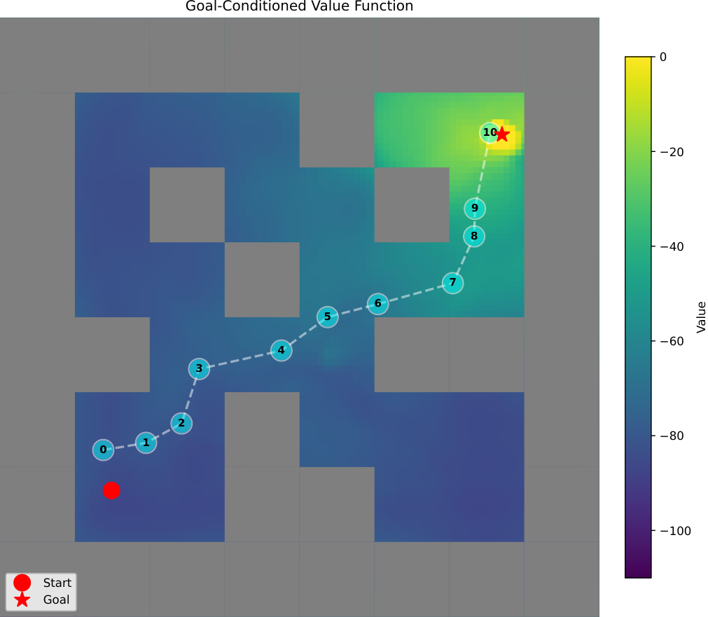
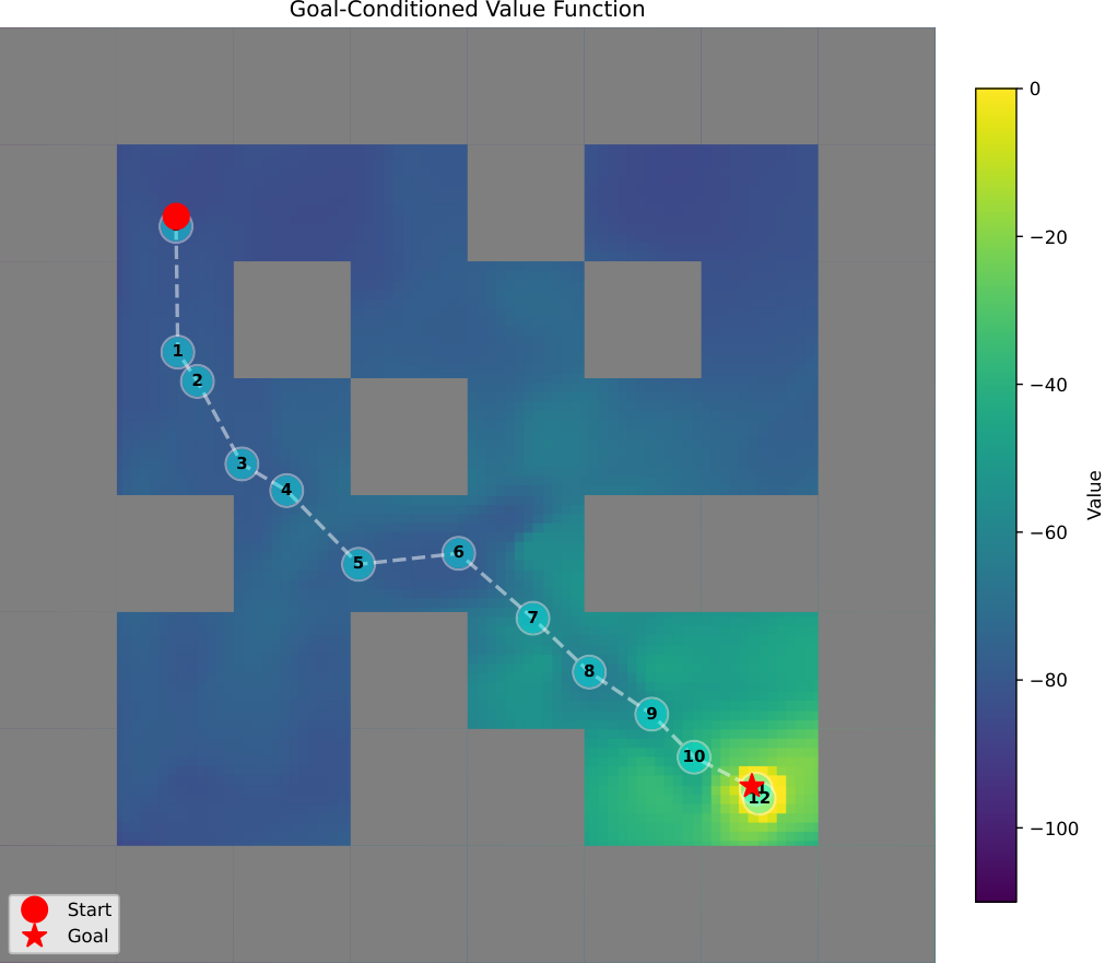
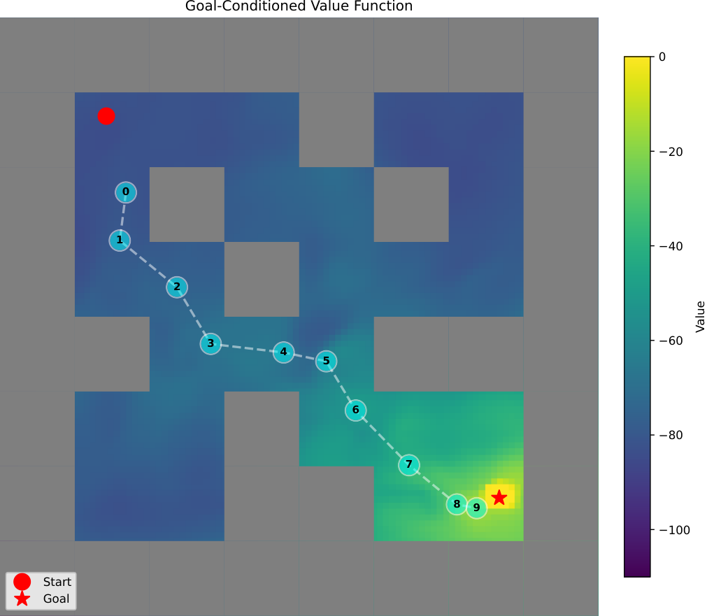
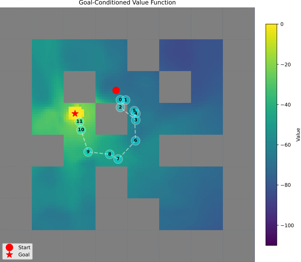
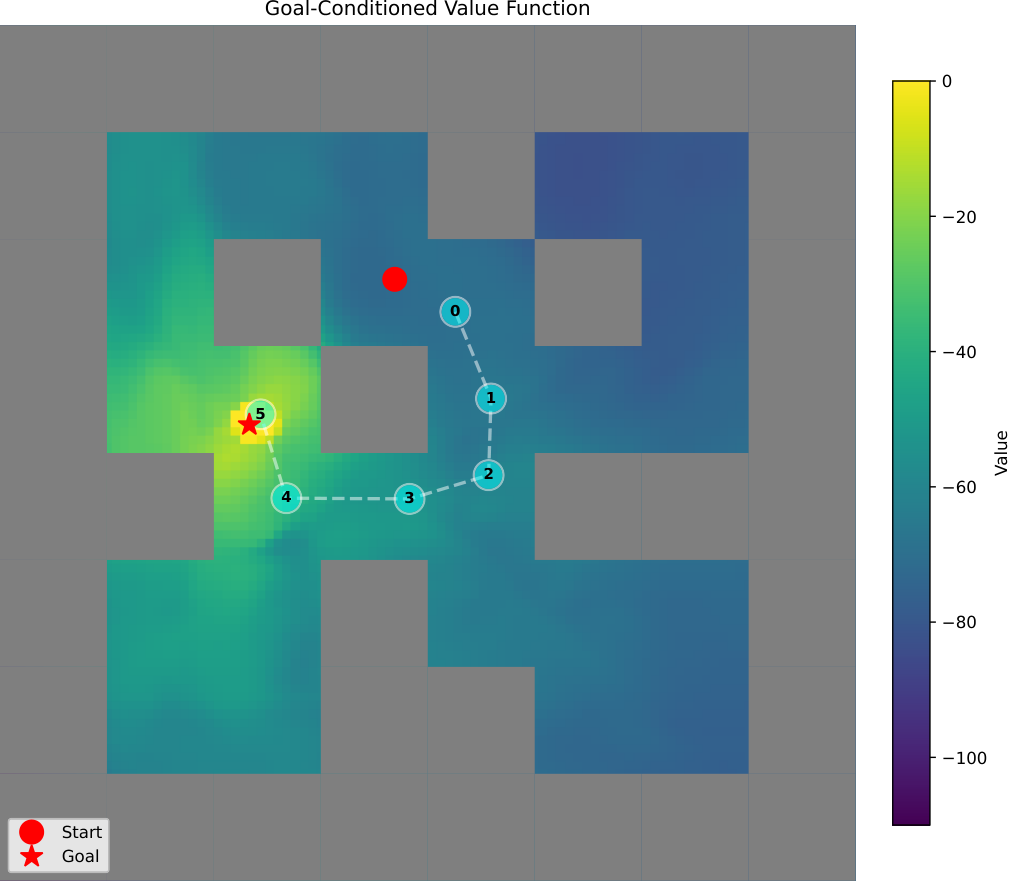
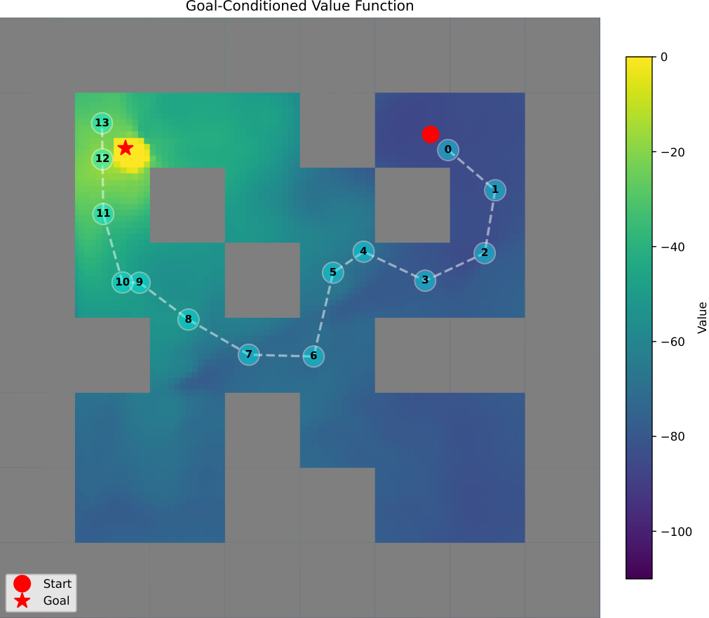
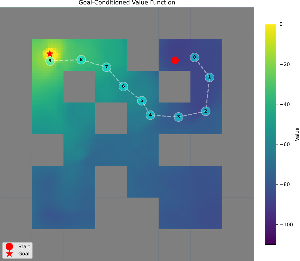
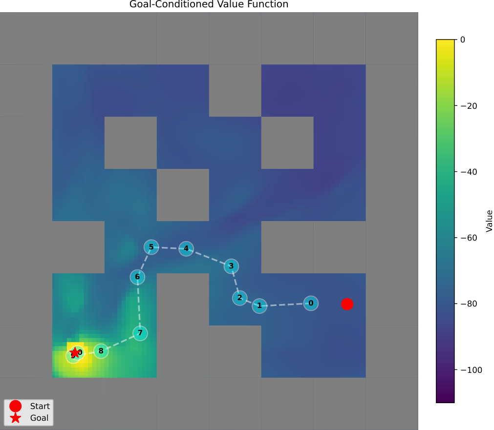
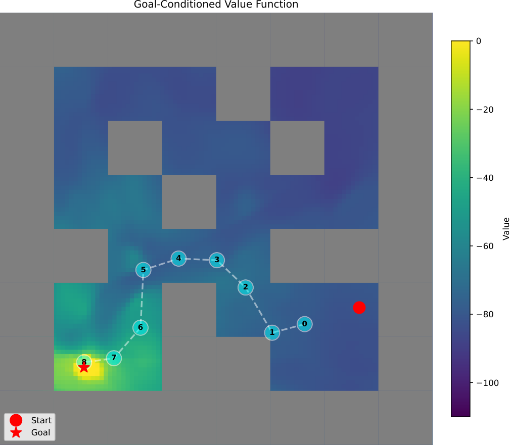
We first visualize the results in the medium-sized maze. As shown in Figure 7, while both methods generally reach the goals, we observe distinct behavioral differences. HIQL^w/o occasionally exhibits artifacts characteristic of value-based planning, such as suboptimal detours or subgoals projected into unreachable areas (e.g., walls). In contrast, DSP produces trajectories that are geometrically consistent and better follow the maze topology, generating smooth paths even in this shorter-horizon setting.

O.2 Large Maze

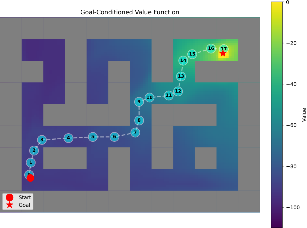
Next, we examine the large-sized maze, where the planning horizon increases. As illustrated in Figure 8, the impact of the horizon becomes visible. HIQL^w/o begins to manifest noticeable detours and inefficient paths, showing less consistent planning as the scale increases. Although the value function eventually corrects the agent’s direction, the guidance is noisy. DSP, however, maintains its planning stability, producing topologically coherent and smooth trajectories without the jaggedness observed in the baseline.

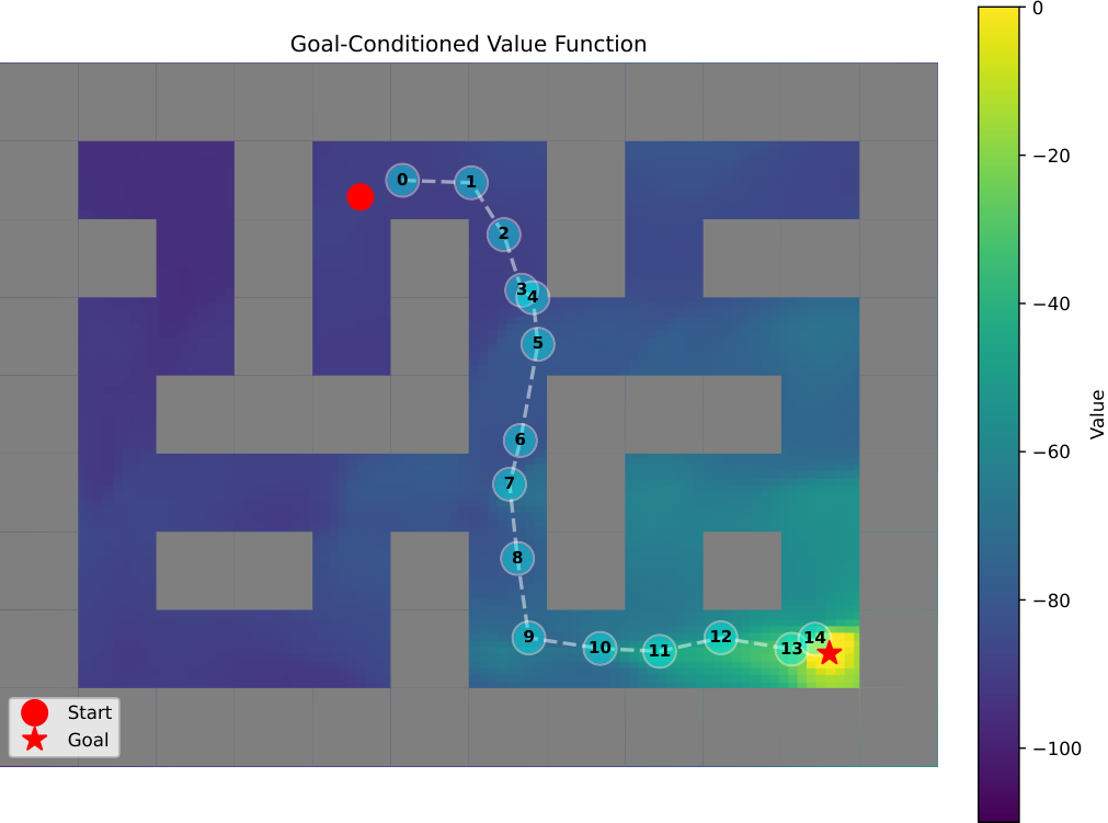
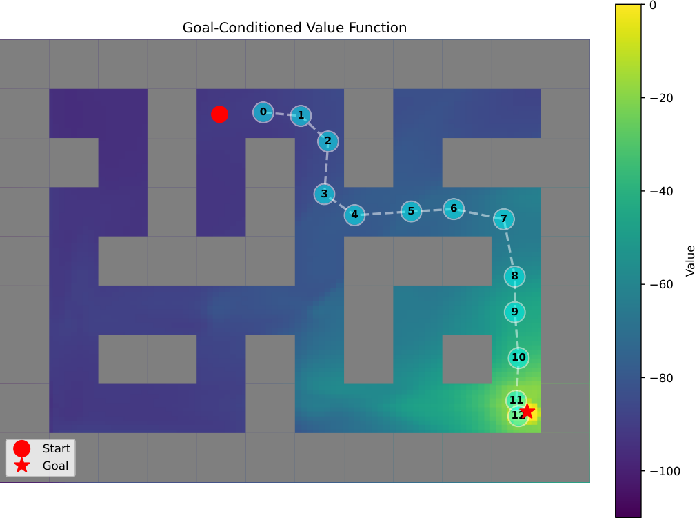
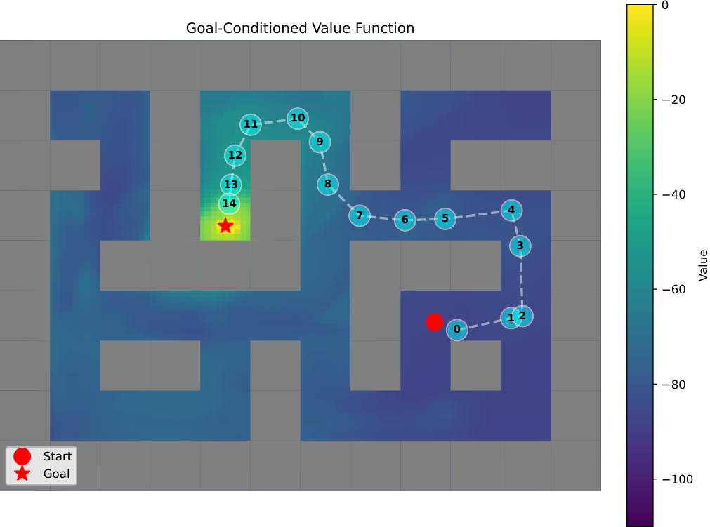
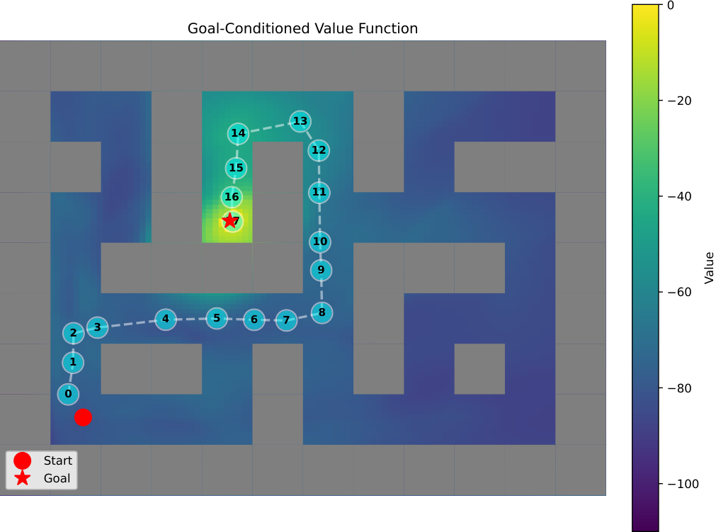
O.3 Giant Maze

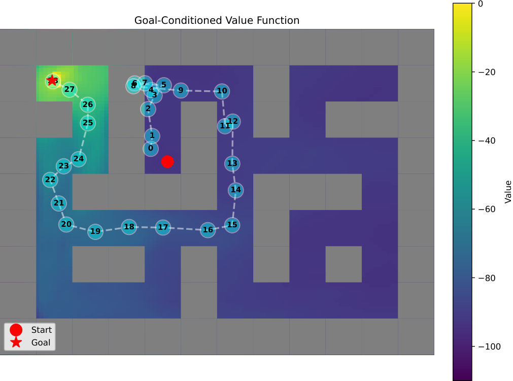
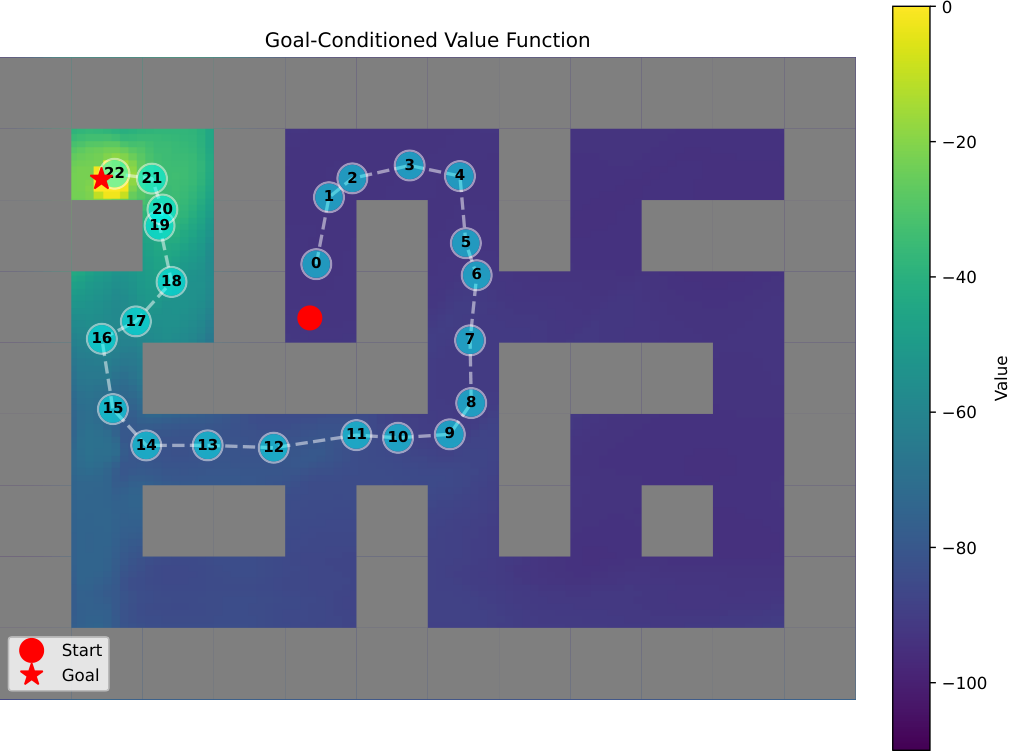
Finally, we extend our visualization to the giant-sized maze, where the curse of horizon is most acute. Here, HIQL^w/o exhibits severe performance degradation. The high-level policy, struggling with the immense scale, often fails to generate valid subgoals, leading to task failure. Even in successful trials, the attenuation of the value signal results in subgoals that linger in local optima; although the agent may eventually escape, the traversal is far from time-optimal.

In sharp contrast, DSP shows more consistent navigation behavior. However, in this extreme setting, we observe a phenomenon of subgoal clustering, where consecutive high-level subgoals are repeatedly generated in a local region. Empirically, this behavior is not indicative of high-level planning failure, as the generated subgoals remain topologically valid and goal-directed. Instead, the clustering pattern demonstrates the planner’s robustness to local execution stochasticity. Since the low-level policy is trained via AWR, it may exhibit minor deviations due to local value approximations. Crucially, unlike the larger global planning errors seen in baselines, these deviations are bounded within short horizons. As a result, the high-level planner successfully re-issues corrective subgoals in the same vicinity to compensate for these local execution errors, ensuring eventual task completion.

Appendix P Comparison Experiments on D4RL Antmaze

To further position DSP with respect to conceptually related diffusion-based hierarchical planning methods, we additionally evaluate DSP on the D4RL AntMaze benchmark. Our main experiments are conducted on OGBench, which is specifically designed for offline goal-conditioned RL and provides broader coverage of long-horizon reasoning, stitching, and stochasticity. By contrast, D4RL AntMaze is more limited for evaluating offline GCRL since it mainly uses a single fixed goal. Nevertheless, D4RL AntMaze is the benchmark on which several prior diffusion-based hierarchical planning methods were originally reported, and therefore provides the most direct setting for comparison.

Table 12: Comparison with diffusion-based hierarchical planning methods on D4RL AntMaze. We report mean

\pm

standard deviation over 5 random seeds, with each seed evaluated on 100 episodes. Baseline numbers are taken from the corresponding original papers when reported under the same D4RL AntMaze setting. The best-performing entry in each row is highlighted in bold.

Datasets	HDMI	DTAMP	HD	SIHD	DSP
antmaze-umaze-v2	$86.1\pm 2.4$	$-$	$-$	$-$	$\mathbf{98.6\pm 2.1}$
antmaze-umaze-diverse-v2	$73.7\pm 1.1$	$-$	$94.0\pm 4.9$	$96.5\pm 2.8$	$\mathbf{96.8\pm 2.6}$
antmaze-medium-play-v2	$-$	$\mathbf{89.3\pm 3.9}$	$-$	$-$	$87.0\pm 3.3$
antmaze-medium-diverse-v2	$-$	$76.7\pm 4.5$	$88.7\pm 8.1$	$92.2\pm 5.0$	$\mathbf{92.4\pm 4.4}$
antmaze-large-play-v2	$-$	$62.0\pm 2.9$	$-$	$-$	$\mathbf{88.8\pm 4.1}$
antmaze-large-diverse-v2	$71.5\pm 3.5$	$53.3\pm 9.7$	$83.6\pm 5.8$	$89.4\pm 4.2$	$\mathbf{95.4\pm 2.9}$

Table 12 compares DSP with representative diffusion-based hierarchical planning baselines, including HDMI [33], DTAMP [21], HD [6], and SIHD [64]. We report mean and standard deviation over 5 random seeds, with each seed evaluated on 100 episodes. Baseline numbers are taken from the corresponding original papers when reported on the same D4RL AntMaze setting. The best-performing entry in each row is highlighted in bold.

Overall, DSP is highly competitive and outperforms prior diffusion-based hierarchical planning methods on most reported tasks. The gains are particularly pronounced on larger and more challenging tasks such as antmaze-large-play-v2 and antmaze-large-diverse-v2, where long-horizon decision errors are more likely to accumulate. On averages over overlapping tasks, DSP substantially outperforms DTAMP (90.9 vs. 70.3) and HDMI (96.9 vs. 77.1), and also improves over HD (94.9 vs. 88.8) and SIHD (94.9 vs. 92.7).

These results are consistent with the key design of DSP. Unlike prior diffusion-based hierarchical planning methods, DSP does not use diffusion as a trajectory- or sequence-level planner. Instead, it models high-level decision making as a goal-conditioned generative subgoal policy. This is consistent with the reduced high-level value-noise path analyzed in Proposition 4.2. At the same time, classifier-free guidance enables direct and controllable goal-directed subgoal selection at inference time, while Proposition 5.1 explains the implicit advantage-weighted bias induced by this guidance.

Appendix Q Dexterous Manipulation Evaluation

We evaluate DSP and HIQL on two bimanual dexterous-manipulation tasks from Bi-DexHands [8]: ShadowHandOver and ShadowHandCatchUnderarm. Using the official collection interface, we construct a fixed offline dataset of $10^{6}$ transitions per task with PPO. Both methods are trained on identical datasets under the same OGBench-style GCRL protocol. HIQL and DSP results are success rates (%) reported as means $\pm$ standard deviations over five seeds. PPO is shown only as a data-collection reference, not as an offline or compute-matched baseline.

The tuples in Table 13 report $(d_{s},d_{a},d_{w},d_{g})$ . The 7D goal $g$ is derived directly from the task-specified target-object pose, while the original 7D waypoint $w$ is a future achieved object pose. To isolate the effect of waypoint dimensionality without changing the final task, we keep the 7D goal fixed and replace the task-space waypoint with a 55/67D task-relevant configuration-space waypoint containing bimanual configuration and object-pose information. Here, $d_{w}$ denotes the waypoint dimension before method-specific processing: HIQL retains its learned subgoal representation, whereas DSP directly generates in the selected waypoint space.

Table 13: Success rates (%) on Bi-DexHands. PPO denotes the data collector. Dimensions are reported as

(d_{s},d_{a},d_{w},d_{g})

Datasets	$(d_{s},d_{a},d_{w},d_{g})$	PPO	HIQL	DSP
ShadowHandOver	$(387,40,7,7)$	46.5	$56.6\pm 4.2$	$\mathbf{74.2}\pm 2.9$
ShadowHandCatchUnderarm	$(411,52,7,7)$	37.2	$46.0\pm 4.1$	$\mathbf{54.6}\pm 3.3$
ShadowHandOver	$(387,40,55,7)$	46.5	$54.2\pm 5.9$	$\mathbf{67.6}\pm 2.4$
ShadowHandCatchUnderarm	$(411,52,67,7)$	37.2	$41.2\pm 3.4$	$\mathbf{46.4}\pm 3.9$

With 7D task-space waypoints, DSP achieves higher mean success than HIQL by 17.6 and 8.6 percentage points on ShadowHandOver and ShadowHandCatchUnderarm, respectively. Moving to 55/67D configuration-space waypoints reduces DSP’s mean success by 6.6/8.2 points, compared with 2.4/4.8 points for HIQL. Nevertheless, DSP retains higher mean success by 13.4/5.2 points in the two higher-dimensional waypoint settings. These results show that waypoint dimensionality is a genuine challenge for direct DSP generation, while providing initial task-specific evidence that its advantage is not solely attributable to the 7D waypoint representation.

The collected datasets contain executable local behaviors. Accordingly, these experiments compare how DSP and HIQL plan and execute bimanual behavior under identical offline data support, rather than testing whether either method can acquire skills absent from the dataset. The results provide initial evidence beyond OGBench’s parallel-jaw manipulation setting, without constituting a comprehensive evaluation of dexterous manipulation.

Diffusion Subgoal Planning for Long-Horizon Offline Goal-Conditioned Reinforcement Learning

Abstract

1 Introduction

2 Related Works

3 Preliminaries

4 High-Level Planning with Reduced Horizon-Dependent Value Noise

4.1 Why Value-Function Noise Limits Long-Horizon Subgoal Planning

Proposition 4.1 (Hierarchical Policy Can Reduce Policy Error [47]).

4.2 Diffusion Subgoal Planning Reduces Horizon-Dependent Value Noise

Proposition 4.2 (Reduced High-Level Value-Noise Amplification).

4.3 Empirical Evidence: DSP Generates More Reliable Subgoals

5 Diffusion Subgoal Planning

5.1 Subgoal Generation as Probabilistic Inference

5.2 Learning the Goal-Directed Velocity Field

5.3 Guided Sampling as Implicit Policy Extraction

Proposition 5.1 (CFG as Implicit Relative-Advantage-Weighted Subgoal Extraction).

5.4 Practical Algorithm

6 Experiments

6.1 Experimental Setup

6.2 Locomotion Results

6.3 Manipulation Results

6.4 Guidance, Data Support, and Executor Reachability

7 Conclusion

Acknowledgments

References

Appendix A Limitations and Future Work

Appendix B Proofs

B.1 Proof of Proposition 4.1

Proof.

B.2 Proof of Proposition 4.2

Proof.

Arbitrary generated subgoals.

Matched-distance DSP error.

Matched-distance HIQL error.

Gaussian directional-error special case.

B.3 Proof of Proposition 5.1

Proof.

Density ratio as normalized goal-reaching value.

Classifier-free guidance as QβQ_{\beta}-weighted extraction.

Appendix C Implementation Details

C.1 Goal Mixed Sampling

C.2 Target Value Network

C.3 Architectures

Appendix D Hyperparameters

Appendix E Computational Resources

Appendix F Environments and Datasets

Appendix G Offline GCRL Baseline Algorithms

Appendix H Subgoal Support and Executor Reachability

Appendix I Hyperparameter Sensitivity

I.1 Guidance Scale

I.2 Diffusion Step

I.3 Subgoal Steps

Appendix J High-Level Subgoal Generation: Ablations and Comparisons

J.1 Controlled Comparison of High-Level Mechanisms

J.2 Comparison with Diffusion-Based Hierarchical Planners

Appendix K Inference-Time Analysis

Appendix L Stitching Experiments

Appendix M Data Coverage and Behavior Quality

M.1 Reduced-Data Coverage

M.2 Official Explore Datasets

Appendix N Evaluation with Visual Observations

Appendix O Visualization of Subgoal Trajectories in Maze Environments

O.1 Medium Maze

O.2 Large Maze

O.3 Giant Maze

Appendix P Comparison Experiments on D4RL Antmaze

Appendix Q Dexterous Manipulation Evaluation

Classifier-free guidance as $Q_{\beta}$ -weighted extraction.