PSM: Dataset Distillation Based on Precise Statistical Matching by Difficulty

Hongxu Ma^1,*, Guang Li^{2,* $\dagger$}, Shijie Wang³, Dongzhan Zhou⁴, Suorong Yang⁵, Baoli Sun⁶, Takahiro Ogawa², Miki Haseyama², Zhihui Wang^{6, $\dagger$} ¹Zhejiang University ²Hokkaido University ³The University of Queensland ⁴Shanghai Artificial Intelligence Laboratory ⁵National University of Singapore ⁶Dalian University of Technology ^*Equal contribution. ^$\dagger$Corresponding authors. guang@lmd.ist.hokudai.ac.jp, zhihuiwang@dlut.edu.cn

Abstract

Dataset distillation (DD) condenses a large original set into a small distilled set with high training utility. Decoupled statistical matching methods substantially reduce distillation time and memory overhead while achieving strong performance. However, they typically supervise all distilled data with running statistics estimated from the entire original set. These statistics mainly capture the average feature distribution while ignoring the difficulty differences among original data, making them insufficient for characterizing the difficulty structure of the original data. To address this issue, we propose Precise Statistical Matching (PSM) by difficulty. After pretraining, PSM uses the Global Precision Score (GPS) to evaluate image difficulty, sorts the original data according to the scores, and then partitions it into IPC (Images Per Class of distilled data) difficulty groups. During distillation, Statistics Updated Again (SUA) updates the teacher’s BN running statistics using original data from each group via forward passes, providing precise supervision with corresponding difficulty for distilled data at each $id_{\mathrm{IPC}}$ . Meanwhile, Initial Sample Screening (ISS) initializes distilled data with original images from the corresponding group, providing an effective starting point for precise matching. Experiments across multiple datasets and model architectures demonstrate the effectiveness of PSM, showing that it broadens the difficulty range of distilled samples and further improves the final performance. Code will be released.

1 Introduction

As datasets grow and neural networks advance, the computational and storage resources required for models have increased substantially (Hoffmann et al., 2022; Sangermano et al., 2022), becoming a major limitation on model development. Dataset distillation (DD) aims to distill a large original set into a small set with high training utility (Lei and Tao, 2024; Liu and Du, 2025), such that models trained on the distilled set can achieve performance comparable to those trained on the original set.

Representative DD methods include gradient matching (Zhao and Bilen, 2021), distribution matching (Li et al., 2026), trajectory matching (Zhong et al., 2025a), generative methods (Gan et al., 2026), and decoupled methods (Shang et al., 2026). Matching methods often rely on bi-level optimization, while generative methods require large generative models, incurring substantial computational and time costs. Recently, decoupled methods (Yin et al., 2023) based on BN (Batch Normalization) statistics matching (Ioffe and Szegedy, 2015) have received increasing attention. By separating teacher pretraining from data distillation, and using the teacher’s BN running statistics to supervise distilled data, they markedly reduce these costs while retaining strong performance.

However, existing decoupled methods typically apply BN running statistics estimated from the entire original set to all distilled data. These global statistics mainly characterize the average feature distribution; uniformly matching them therefore smooths out the representation differences between easy and hard data. As shown in Figure 1(a), the data distilled by FADRM exhibit visually similar difficulty, and Figure 1(b) further reveals that their difficulty remains nearly constant. Consequently, the distilled data cannot adequately cover the range of feature distributions spanned by original data of varying difficulty, limiting the student’s ability to learn the difficulty structure of the original data.

To address this limitation, we propose Precise Statistical Matching (PSM) by difficulty. To align difficulty estimation with statistical matching in the same feature space, we carefully design the Global Precision Score (GPS): after pretraining, for each original image, GPS computes statistics at the inputs to the teacher’s BN layers, and then measures image difficulty as their distance from the corresponding BN running statistics (under the ensemble-based paradigm, PSM averages the GPS rankings of all teachers to integrate their judgments); a higher GPS indicates greater deviation from the average feature distribution, and thus greater difficulty; based on the GPS ranking, PSM then partitions the original data within each class into IPC (Images per Class) difficulty groups.

During distillation, when optimizing the $g$ -th batch of distilled data, Statistics Updated Again (SUA) feeds original data from the $g$ -th group through the teacher to update its BN running statistics via forward propagation, producing supervision that more accurately characterizes the current difficulty group. Initial Sample Screening (ISS) selects real images from the same group to initialize the distilled data, aligning their initial difficulty with the target group. Together, SUA and ISS construct statistical supervision and initialization for different difficulty groups, enabling the distilled data to cover a broader difficulty range, and helping the student to learn a more complete difficulty structure.

Extensive experiments on multiple datasets demonstrate that PSM outperforms existing state-of-the-art (SOTA) methods, validating its effectiveness. Our contributions are summarized as follows:

•

We revisit the existing decoupled DD paradigm, in which BN running statistics estimated from the original set serve as supervision signals, and show that this paradigm limits variation in difficulty within the distilled data. To address this issue, we propose GPS, a difficulty metric closely aligned with statistical supervision, to rank the original data by difficulty.
•

We propose PSM, a method that broadens the range of difficulty covered by the distilled data by adjusting statistical supervision and initial data: SUA updates the teacher model’s BN running statistics through forward propagation; ISS selects original images from the corresponding difficulty group to initialize the distilled data.
•

We conducted experiments on multiple datasets and model architectures, and the results show that PSM broadens the difficulty range of distilled samples, further improving the final performance and demonstrating its effectiveness.

2 Related Work

Dataset distillation (DD) compresses a large dataset into a small set of samples with high training utility, reducing storage and training costs while retaining performance comparable to training on the full dataset. Existing methods mainly include gradient matching (Lee et al., 2022; Liu et al., 2023), distribution matching (Zhao and Bilen, 2023; Li et al., 2025c), trajectory matching (Chen et al., 2023; Guo et al., 2024), decoupled distillation (Yin and Shen, 2024; Xiao and He, 2024), and generative distillation (Zhong et al., 2025b; Cai et al., 2026). Further related work is discussed in the appendix A.

3 Preliminaries

3.1 Dataset Distillation

Let $\mathcal{T}=\{(x_{i},y_{i})\}_{i=1}^{N}$ denote the original set, and let $\mathcal{D}=\{(\tilde{x}_{j},\tilde{y}_{j})\}_{j=1}^{M}$ denote the distilled set, where $M\ll N$ . Let $\theta_{\mathcal{T}}$ and $\theta_{\mathcal{D}}$ represent the parameters obtained by training on $\mathcal{T}$ and $\mathcal{D}$ , respectively. DD aims to construct $\mathcal{D}$ such that models trained on $\mathcal{D}$ achieve performance comparable to those trained on $\mathcal{T}$ . Given a distillation budget $M$ , this objective can be formulated as

\mathcal{D}^{*}=\operatorname*{arg\,min}_{\mathcal{D}:\,|\mathcal{D}|=M}\sup_{(x,y)\in\mathcal{T}}\left|\mathcal{L}\!\left(f_{\theta_{\mathcal{T}}}(x),y\right)-\mathcal{L}\!\left(f_{\theta_{\mathcal{D}}}(x),y\right)\right|,

(1)

where $\mathcal{L}(\cdot,\cdot)$ denotes the task loss. Under a given distillation budget, the number of images per class (IPC) is the same across all classes. Typically, a student trained on the distilled set is evaluated on the original test set, and its test performance is used to measure the quality of the distilled set.

3.2 Decoupled Dataset Distillation

SRe²L (Yin et al., 2023) introduced a three-stage framework that separates model training from data distillation. During distillation, the pretrained teacher is fixed, and only the distilled data are optimized, avoiding the inner optimization of model parameters and reducing computational overhead.

I. Teacher model pretraining.

The teacher is trained on the original set $\mathcal{T}$ to learn feature representations, while its BN layers accumulate running means and variances from the training data. The resulting parameters $\theta_{\mathcal{T}}$ and BN statistics are then fixed to guide distillation.

II. Distillation.

A distilled batch $\widetilde{\mathcal{B}}={(\tilde{x}_{j},\tilde{y}_{j})}_{j=1}^{B}$ is fed into the frozen teacher, where $B$ is typically equal to the number of classes $C$ . The classification loss $\mathcal{L}_{\mathrm{cls}}$ enforces semantic consistency, while the statistics matching loss $\mathcal{L}_{\mathrm{BN}}$ aligns the batch statistics with the teacher’s running statistics:

$\displaystyle\mathcal{L}_{\mathrm{dist}}(\widetilde{\mathcal{B}})$	$\displaystyle=\mathcal{L}_{\mathrm{cls}}\left(\tilde{x},\tilde{y}\right)+\lambda_{\mathrm{BN}}\mathcal{L}_{\mathrm{BN}}\left(\{\tilde{x}_{j}\}_{j=1}^{B}\right),$	(2)
$\displaystyle\text{where}\quad\mathcal{L}_{\mathrm{cls}}\left(\tilde{x},\tilde{y}\right)$	$\displaystyle=\mathbb{E}_{(\tilde{x},\tilde{y})\sim\widetilde{\mathcal{B}}}\left[\mathcal{L}_{\mathrm{CE}}\left(f_{\theta_{\mathcal{T}}}(\tilde{x}),\tilde{y}\right)\right],$
$\displaystyle\mathcal{L}_{\mathrm{BN}}\left(\{\tilde{x}_{j}\}_{j=1}^{B}\right)$	$\displaystyle={\textstyle\sum_{\ell=1}^{L}}\left(\left\\|{\mu}_{\ell}-\bar{\mu}_{\ell}\right\\|_{2}+\left\\|{\sigma}_{\ell}^{2}-\bar{\sigma}_{\ell}^{2}\right\\|_{2}\right),$

where $\mathcal{L}_{\mathrm{CE}}$ is the cross entropy loss; $\lambda_{\mathrm{BN}}$ weights statistics matching; and $L$ is the number of BN layers, indexed by $\ell$ . For a BN layer with $C_{\ell}$ channels, $\mu_{\ell},\sigma_{\ell}^{2}\in\mathbb{R}^{C_{\ell}}$ are the batch mean and variance at its input, while $\bar{\mu}_{\ell},\bar{\sigma}_{\ell}^{2}\in\mathbb{R}^{C_{\ell}}$ are the corresponding teacher running statistics.

III. Soft label generation.

The distilled data are fed into the pretrained teacher, whose class probability distributions are used as soft labels. These labels also preserve semantic relationships for all classes. The student is then trained on the distilled data and soft labels, receiving richer supervision.

3.3 Batch Normalization

Batch Normalization (BN) (Ioffe and Szegedy, 2015) was originally introduced to mitigate changes in intermediate feature distributions. For features entering a BN layer, BN first computes the mean and variance of the current batch for each channel, and uses them to normalize the features. This process stabilizes feature scales across layers and improves optimization stability.

During training, each BN layer uses the current batch statistics for feature normalization, and its running mean and variance are continuously updated through an exponential moving average. Given the training batch $\mathcal{B}_{t}$ at step $t$ , the running statistics of BN layer $\ell$ are updated as follows:

\bar{\mu}_{\ell,t}=(1-\rho)\bar{\mu}_{\ell,t-1}+\rho\mu_{\ell}(\mathcal{B}_{t}),\qquad\bar{\sigma}_{\ell,t}^{2}=(1-\rho)\bar{\sigma}_{\ell,t-1}^{2}+\rho\sigma_{\ell}^{2}(\mathcal{B}_{t}),

(3)

where $\rho\in(0,1]$ controls the statistics update, a larger $\rho$ assigns more weight to the current batch.

4 Method

4.1 Limitations of Decoupled Dataset Distillation

SRe²L (Yin et al., 2023) pioneered the decoupled DD paradigm, which uses the BN running statistics stored in a pretrained teacher as supervisory signals to guide the optimization, as shown in equation 2. Because of its efficiency, this paradigm has attracted considerable attention. Recent studies have improved this paradigm by reducing storage overhead (Cui et al., 2026), lowering computational complexity (Shang et al., 2026), and enhancing performance (Shi et al., 2026). However, most of these studies rely on additional components or optimization mechanisms, with limited attention paid to the fundamental supervisory signals and their influence.

Homogeneous Supervision.

Existing decoupled methods use the global BN running statistics stored in the pretrained teacher as the target for every distilled batch. Let $\bm{\tau}_{g}$ denote the statistical supervision assigned to batch $g$ , and let $\bm{\tau}^{\mathrm{G}}$ denote the global BN statistics. Then

\tau_{g}=\tau^{\mathrm{G}},\ \forall g\quad\Longrightarrow\quad\mathcal{D}_{\mathrm{sup}}(\tau_{g},\tau_{h})=0,\ \forall g,h.

Consequently, the statistical target is independent of the batch index, and cannot explicitly provide batch-specific difficulty supervision. Although initialization and optimization may introduce difficulty variation, this variation is not controlled by the supervision signal, making it difficult to preserve the difficulty structure of the original data, as illustrated in Figure 1(b).

4.2 Dataset Distillation Based on Precise Statistical Matching by Difficulty

Figure 2 illustrates the overall pipeline of the proposed method. Given the original set and a pretrained teacher, we first employ GPS to evaluate the difficulty of each original data point and rank the data within each class from easy to hard. We then divide the ordered data of each class into $\mathrm{IPC}$ difficulty groups, with different groups representing data of varying difficulty in the original set. When distilling the $g$ -th batch, SUA feeds the original data in difficulty group $g$ into the teacher to further adapt its BN running statistics to the characteristics of the current group, thereby constructing distinct statistical supervision signals for the corresponding distilled batch. By matching the respective statistical supervision signals, the distilled data in different batches progressively learn original data patterns from easy to hard. Meanwhile, ISS selects original data from the corresponding difficulty group to initialize the distilled data, aligning the difficulty of the initial data with that of the target distilled batch, and providing a favorable starting point for subsequent optimization. GPS, SUA, and ISS are introduced in the following sections. See the appendix D for pseudocode.

4.2.1 GPS: Global Precision Score

To accurately partition the original set by difficulty and ensure that difficulty estimation and BN statistics operate in the same feature space, we propose a new difficulty partitioning method, GPS.

Operation and Purpose.

We compute the per-channel mean and variance of $x_{i}$ at the input to each BN layer, and compare them with the corresponding running mean and variance. GPS is defined as

\operatorname{GPS}(x_{i})=\mathbb{E}_{k\in\{1,\ldots,K\}}\left[\operatorname{rank}_{c}\left(\mathbb{E}_{\ell\in\{1,\ldots,L_{k}\}}\left[\frac{\left\|\bm{\mu}_{\ell,i,k}-\bar{\bm{\mu}}_{\ell,k}\right\|_{2}+\beta\left\|\log\frac{\bm{\sigma}_{\ell,i,k}^{2}+\epsilon}{\bar{\bm{\sigma}}_{\ell,k}^{2}+\epsilon}\right\|_{2}}{\sqrt{C_{\ell,k}}}\right]\right)\right].

(4)

Here $K$ denotes the number of teachers, $\operatorname{rank}{c}(\cdot)$ is the rank of a sample within class $c$ , $\beta$ balances the mean and variance distances, and $\epsilon$ ensures numerical stability. For the variance, we first compute the ratio between the sample variance and the BN running variance to reduce the effect of variance scale differences across channels. We then take the logarithm of this ratio to stabilize its numerical range. Finally, we normalize the statistical distance at each layer by $\sqrt{C_{\ell,k}}$ to reduce distance scale discrepancies caused by the number of channels across BN layers.

A larger GPS indicates that the data exhibits more pronounced statistical deviations across multiple feature layers, and thus corresponds to greater difficulty. Based on the GPS ranking, PSM divides the ordered data of each class into IPC difficulty groups of approximately equal size, which sequentially represent the original data from easy to hard. The resulting difficulty groups provide the basis for SUA to construct distinct supervision, and for ISS to select the corresponding initialization data.

Empirical Observation.

A larger GPS indicates more pronounced deviations between the sample statistics and the teacher’s BN running statistics. To verify the correlation between statistics deviations and classification difficulty, we sort the original samples in ascending order of GPS, and compute the teacher’s cross-entropy loss on each sample’s ground truth label. The empirical relationship between GPS and classification difficulty is expressed as

\operatorname{GPS}(x_{i})\uparrow\quad\Longrightarrow\quad\mathcal{L}_{\mathrm{CE}}\!\left(f_{\theta}(x_{i}),y_{i}\right)=-\log p_{\theta}(y_{i}\mid x_{i})\uparrow.

(5)

Experimental results show that the cross-entropy loss generally increases along the GPS ranking. Samples with larger GPS values tend to have higher classification losses. These results indicate that GPS effectively reflects the sample difficulty perceived by the teacher, providing a basis for grouping samples from easy to hard. A detailed analysis is provided in the appendix B.1.

4.2.2 SUA: Statistics Updated Again

To convert the difficulty groups obtained by GPS into statistical supervision corresponding to individual distillation batches, we propose SUA.

Operation and Purpose.

Let $\mathcal{T}_{g}$ denote the $g$ -th difficulty group. We set $\mathrm{IPC}$ difficulty groups, with the $g$ -th group corresponding to the $id_{\mathrm{IPC}}$ -th distillation batch. For teacher $k$ , SUA starts from the global BN running statistics $\bm{\tau}_{k}^{\mathrm{G}}$ stored in the pretrained teacher, freezes the teacher parameters $\theta_{k}$ , and performs $\left\lfloor r_{\mathrm{fwd}}E_{k}^{\mathrm{pre}}\right\rfloor$ epochs of forward propagation over $\mathcal{T}_{g}$ . During this process, only the BN running statistics are updated according to equation 3. This process is expressed as

\bm{\tau}_{k}^{\mathrm{G}}\mathrel{\raisebox{-3.01385pt}{$\xrightarrow{f_{\theta_{k}=\mathrm{constant}}^{\left\lfloor r_{\mathrm{fwd}}E_{k}^{\mathrm{pre}}\right\rfloor}(\mathcal{T}_{g})}$}}\bm{\tau}_{k,g}^{\mathrm{SUA}}.

(6)

where $r_{\mathrm{fwd}}$ denotes the ratio of forward propagation epochs, $E_{k}^{\mathrm{pre}}$ denotes the number of pretraining epochs for teacher $k$ , $\left\lfloor r_{\mathrm{fwd}}E_{k}^{\mathrm{pre}}\right\rfloor$ denotes the actual number of forward propagation epochs, and $\bm{\tau}_{k,g}^{\mathrm{SUA}}$ denotes the BN running statistics obtained by SUA.

Through this update, the BN running statistics of the teacher gradually approach those of the current difficulty group, and serve as the statistical matching signal for distillation batch $g$ , thereby providing each distillation batch with supervision signal corresponding to its difficulty.

Proposition 1 (Expected Convergence; Proof in Appendix B.2).

For any fixed teacher $k$ , let $\bm{\tau}_{k,g}^{\star}$ and $\bm{\tau}_{k,g}^{(t)}$ denote the expected BN batch statistics of $\mathcal{T}_{g}$ and the running statistics after $t$ forward batch updates, respectively. If the forward batches are independently drawn from $\mathcal{T}_{g}$ , then

\mathbb{E}\left[\bm{\tau}_{k,g}^{(t)}\right]-\bm{\tau}_{k,g}^{\star}=(1-\rho)^{t}\left(\bm{\tau}_{k}^{\mathrm{G}}-\bm{\tau}_{k,g}^{\star}\right)\xrightarrow{t\rightarrow\infty}\bm{0}.

(7)

Thus, SUA statistics converge in expectation to those of the current difficulty group. The updated statistics then serve as the matching signal for batch $g$ , guiding its distilled data to match the corresponding feature statistics.

4.2.3 ISS: Initial Sample Screening

The initialization of distilled data significantly affects final performance. EDC (Shao et al., 2024b) shows that real image initialization reduces the distribution gap between the initialized and original data. SelMatch (Lee and Chung, 2024) further shows that real samples of appropriate difficulty help introduce corresponding complex features. Motivated by these findings, we propose ISS to initialize each distillation batch with real data matching its target difficulty.

Specifically, let $\mathcal{T}_{g,c}$ denote the original data of class $c$ in difficulty group $g$ . ISS further selects real images from $\mathcal{T}_{g,c}$ based on their difficulty, and uses them to initialize the distilled data $\widetilde{x}_{g,c}^{(0)}$ . Since the initialization images and the statistical supervision come from the same difficulty group, they are aligned in difficulty, reducing the statistical bias at the beginning of optimization. Experiments show that ISS significantly improves final distillation performance.

5 Experiments

5.1 Experimental Setup

Baselines.

FADRM (Cui et al., 2025a) is a recent SOTA method for decoupled DD, achieving improved performance while substantially reducing memory and time costs, we therefore adopt it as our primary baseline and further compare with FADRM+, its extension using multiple models. SRe²L (Yin et al., 2023), a representative foundational method for decoupled DD, is also included for comparison. In addition, we include RDED (Sun et al., 2024) as a representative method from other DD paradigms, it constructs distilled data by assembling real images, which has been adopted by other DD methods for distilled data initialization.

Datasets.

We evaluate PSM on benchmark datasets widely used in dataset distillation. For low resolution datasets, we use CIFAR-10/100 (Krizhevsky, 2009) at $32\times 32$ , and Tiny-ImageNet (Le and Yang, 2015) at $64\times 64$ . For high-resolution datasets, we mainly use ImageNet-1K (Deng et al., 2009) at $224\times 224$ and its subsets, ImageWoof (fine-grained dataset) and ImageNette.

Implementation Details.

For PSM, we follow the post-evaluation protocol of FADRM. Students are trained for 1000 epochs on Tiny-ImageNet with $\mathrm{IPC}=1$ and CIFAR-10/100, and for 300 epochs in all other settings. For a fair comparison with FADRM+, we further adopt the multi-teacher variant PSM+, which consistently employs ShuffleNetV2 (Ma et al., 2018), ResNet18 (He et al., 2016), MobileNetV2 (Sandler et al., 2018), and DenseNet121 (Huang et al., 2017) as teachers for distillation across all datasets. The remaining parameters are kept consistent with FADRM, while other baselines follow their original settings. See the appendix D for more details.

5.2 Comparison With State-of-The-Art Methods

5.2.1 Main Results

In Table 1, methods marked with “+” use multiple teachers for distillation and a single student for evaluation, while the remaining methods follow the standard same-architecture evaluation protocol.

Low-resolution datasets.

As shown in Table 1, we evaluate PSM on CIFAR-10/100 and Tiny-ImageNet. The results show that PSM outperforms its corresponding baselines in most settings when evaluated with ResNet18/50. Notably, on CIFAR-10 with $\mathrm{IPC}=10$ , PSM achieves a Top-1 accuracy of 52.7% with ResNet50, outperforming FADRM by 8.9%, and demonstrating the effectiveness of PSM. On CIFAR-10 with $\mathrm{IPC}=1$ , PSM performs comparably to its corresponding baselines. This may be mainly attributed to CIFAR-10 containing only 10 coarse categories, for which the global statistics may already adequately characterize the overall difficulty distribution. Consequently, SUA induces only limited changes in the statistics, resulting in small performance differences.

High-resolution datasets.

We evaluate PSM on ImageNette, ImageWoof, and ImageNet-1K. As shown in Table 1, PSM achieves consistent performance gains in most settings, demonstrating its strong robustness. Performance degradation occurs mainly on ImageWoof with ResNet50 as the student under the $\mathrm{IPC}=1/10$ . One possible explanation is the limited compatibility of ResNet50 with ImageWoof: when trained on the original set, ResNet18 achieves an accuracy of 85.0%, whereas ResNet50 achieves only 80.3%. Under low IPC, the limited distilled data may further amplify this mismatch, making it difficult for ResNet50 to learn the difficulty information preserved by PSM.

Table 1: Top-1 accuracy comparison of PSM, extended variant PSM+, and other SOTA methods. For each dataset, IPC, and student setting, the mean values of the best and second best results are marked in bold and underlined, respectively. Values in parentheses after the PSM and PSM+ results indicate their performance changes relative to FADRM and FADRM+, respectively.

Student

ResNet18

ResNet50 (He et al., 2016)

Dataset

IPC

SRe²L

RDED

FADRM

PSM

FADRM+

PSM+

SRe²L

RDED

FADRM

PSM

FADRM+

PSM+

CIFAR-10

16.6_{\pm 0.9}

\underline{22.9}_{\pm 0.4}

19.3_{\pm 0.6}

20.9_{\pm 0.1}

(\uparrow 1.6)

\textbf{23.7}_{\pm 0.8}

22.3_{\pm 0.6}

(\downarrow 1.4)

15.2_{\pm 1.3}

19.7_{\pm 1.7}

23.2_{\pm 0.7}

23.2_{\pm 0.2}

(=0.0)

\textbf{23.5}_{\pm 1.3}

\underline{23.3}_{\pm 0.4}

(\downarrow 0.2)

29.3_{\pm 0.5}

37.1_{\pm 0.3}

48.2_{\pm 0.4}

54.5_{\pm 1.3}

(\uparrow 6.3)

\underline{55.9}_{\pm 1.0}

\textbf{61.1}_{\pm 0.8}

(\uparrow 5.2)

30.3_{\pm 1.7}

32.5_{\pm 0.9}

43.8_{\pm 1.1}

52.7_{\pm 0.1}

(\uparrow 8.9)

\underline{55.1}_{\pm 0.8}

\textbf{56.8}_{\pm 1.1}

(\uparrow 1.7)

45.0_{\pm 0.7}

62.1_{\pm 0.1}

80.6_{\pm 0.7}

81.1_{\pm 0.1}

(\uparrow 0.5)

\underline{85.8}_{\pm 0.1}

\textbf{86.7}_{\pm 0.2}

(\uparrow 0.9)

52.9_{\pm 1.3}

52.5_{\pm 2.0}

79.7_{\pm 1.2}

82.7_{\pm 0.7}

(\uparrow 3.0)

\underline{83.7}_{\pm 0.6}

\textbf{86.0}_{\pm 0.9}

(\uparrow 2.3)

Whole dataset

92.9

93.1

CIFAR-100

6.6_{\pm 0.2}

11.1_{\pm 0.3}

31.3_{\pm 0.2}

32.9_{\pm 0.9}

(\uparrow 1.6)

\underline{37.9}_{\pm 0.8}

\textbf{39.1}_{\pm 0.1}

(\uparrow 1.2)

6.0_{\pm 0.1}

11.6_{\pm 0.4}

24.4_{\pm 1.6}

26.2_{\pm 1.4}

(\uparrow 1.8)

\underline{33.6}_{\pm 0.8}

\textbf{34.9}_{\pm 1.3}

(\uparrow 1.3)

27.0_{\pm 0.4}

42.6_{\pm 0.2}

64.7_{\pm 0.4}

\textbf{66.7}_{\pm 0.4}

(\uparrow 2.0)

62.5_{\pm 0.2}

\underline{66.1}_{\pm 0.2}

(\uparrow 3.6)

35.4_{\pm 1.9}

50.3_{\pm 0.4}

61.8_{\pm 0.5}

\underline{64.6}_{\pm 0.1}

(\uparrow 2.8)

62.3_{\pm 0.2}

\textbf{65.7}_{\pm 0.4}

(\uparrow 3.4)

50.2_{\pm 0.4}

62.6_{\pm 0.1}

69.3_{\pm 0.3}

\underline{69.7}_{\pm 0.3}

(\uparrow 0.4)

67.4_{\pm 0.4}

\textbf{70.1}_{\pm 0.1}

(\uparrow 2.7)

52.9_{\pm 0.1}

66.8_{\pm 0.3}

67.6_{\pm 0.5}

\underline{69.8}_{\pm 0.1}

(\uparrow 2.2)

68.2_{\pm 0.1}

\textbf{70.7}_{\pm 0.2}

(\uparrow 2.5)

Whole dataset

73.6

74.4

Tiny-ImageNet

2.6_{\pm 0.1}

9.7_{\pm 0.4}

28.6_{\pm 0.1}

30.6_{\pm 1.3}

(\uparrow 2.0)

\underline{32.4}_{\pm 0.2}

\textbf{35.4}_{\pm 0.7}

(\uparrow 3.0)

5.1_{\pm 0.1}

6.5_{\pm 0.5}

31.1_{\pm 0.4}

\underline{31.3}_{\pm 0.7}

(\uparrow 0.2)

31.0_{\pm 1.3}

\textbf{32.9}_{\pm 0.9}

(\uparrow 1.9)

16.1_{\pm 0.2}

41.9_{\pm 0.2}

46.5_{\pm 0.4}

\underline{48.1}_{\pm 0.3}

(\uparrow 1.6)

47.3_{\pm 1.1}

\textbf{48.4}_{\pm 0.3}

(\uparrow 1.1)

43.0_{\pm 0.5}

36.9_{\pm 0.4}

47.5_{\pm 0.3}

\underline{48.0}_{\pm 0.3}

(\uparrow 0.5)

47.1_{\pm 0.4}

\textbf{48.2}_{\pm 0.9}

(\uparrow 1.1)

41.1_{\pm 0.4}

\textbf{58.2}_{\pm 0.1}

51.4_{\pm 0.1}

51.7_{\pm 0.1}

(\uparrow 0.3)

52.0_{\pm 1.0}

\underline{52.1}_{\pm 0.1}

(\uparrow 0.1)

58.3_{\pm 0.1}

48.0_{\pm 0.8}

\textbf{57.8}_{\pm 0.1}

\underline{56.6}_{\pm 0.7}

(\downarrow 1.2)

52.2_{\pm 1.8}

53.0_{\pm 0.2}

(\uparrow 0.8)

Whole dataset

60.3

63.4

ImageNette

19.1_{\pm 1.1}

\textbf{35.8}_{\pm 1.0}

28.2_{\pm 0.6}

25.0_{\pm 0.5}

(\downarrow 3.2)

30.5_{\pm 1.3}

\underline{32.5}_{\pm 0.5}

(\uparrow 2.0)

13.6_{\pm 0.5}

23.6_{\pm 1.4}

23.7_{\pm 0.4}

22.9_{\pm 0.8}

(\downarrow 0.8)

\underline{25.5}_{\pm 0.7}

\textbf{29.2}_{\pm 0.6}

(\uparrow 3.7)

29.4_{\pm 3.0}

61.4_{\pm 0.4}

64.0_{\pm 0.1}

67.1_{\pm 0.2}

(\uparrow 3.1)

\underline{68.5}_{\pm 0.4}

\textbf{69.4}_{\pm 0.8}

(\uparrow 0.9)

32.5_{\pm 1.1}

52.6_{\pm 2.8}

60.9_{\pm 0.5}

62.4_{\pm 0.4}

(\uparrow 1.5)

\underline{66.3}_{\pm 0.8}

\textbf{67.6}_{\pm 0.5}

(\uparrow 1.3)

40.9_{\pm 0.3}

80.4_{\pm 0.4}

82.8_{\pm 0.6}

84.0_{\pm 0.3}

(\uparrow 1.2)

\underline{84.6}_{\pm 0.7}

\textbf{85.1}_{\pm 0.3}

(\uparrow 0.5)

60.8_{\pm 1.0}

74.5_{\pm 2.5}

81.6_{\pm 0.4}

82.3_{\pm 0.3}

(\uparrow 0.7)

\underline{85.4}_{\pm 0.3}

\textbf{85.9}_{\pm 0.2}

(\uparrow 0.5)

Whole dataset

90.2

89.1

ImageWoof

13.3_{\pm 0.5}

\textbf{20.8}_{\pm 1.2}

19.3_{\pm 0.3}

\underline{20.2}_{\pm 0.7}

(\uparrow 0.9)

19.4_{\pm 0.5}

14.9_{\pm 0.9}

(\downarrow 4.5)

12.2_{\pm 2.2}

\underline{21.1}_{\pm 1.9}

\textbf{21.6}_{\pm 0.5}

16.5_{\pm 0.7}

(\downarrow 5.1)

18.4_{\pm 0.2}

15.1_{\pm 0.7}

(\downarrow 3.3)

20.2_{\pm 0.2}

38.5_{\pm 2.1}

43.8_{\pm 0.2}

44.5_{\pm 0.5}

(\uparrow 0.7)

\underline{47.2}_{\pm 0.2}

\textbf{48.3}_{\pm 0.6}

(\uparrow 1.1)

19.8_{\pm 1.4}

40.9_{\pm 3.1}

37.8_{\pm 0.6}

34.0_{\pm 1.0}

(\downarrow 3.8)

\textbf{44.9}_{\pm 0.9}

\underline{43.5}_{\pm 1.2}

(\downarrow 1.4)

23.3_{\pm 0.3}

68.5_{\pm 0.7}

67.7_{\pm 1.0}

69.6_{\pm 0.9}

(\uparrow 1.9)

\underline{73.0}_{\pm 0.6}

\textbf{74.4}_{\pm 0.5}

(\uparrow 1.4)

35.7_{\pm 0.4}

59.8_{\pm 3.2}

66.5_{\pm 1.1}

68.0_{\pm 1.0}

(\uparrow 1.5)

\underline{72.7}_{\pm 0.7}

\textbf{73.7}_{\pm 0.7}

(\uparrow 1.0)

Whole dataset

80.3

ImageNet-1K

21.3_{\pm 0.6}

42.0_{\pm 0.1}

47.8_{\pm 0.4}

48.8_{\pm 0.2}

(\uparrow 1.0)

\underline{50.8}_{\pm 0.1}

\textbf{51.6}_{\pm 0.3}

(\uparrow 0.8)

28.4_{\pm 0.1}

–

45.6_{\pm 1.6}

45.3_{\pm 0.8}

(\downarrow 0.3)

\underline{56.9}_{\pm 0.2}

\textbf{57.1}_{\pm 0.5}

(\uparrow 0.2)

46.8_{\pm 0.2}

56.5_{\pm 0.1}

\underline{60.9}_{\pm 0.1}

\textbf{61.3}_{\pm 0.1}

(\uparrow 0.4)

59.2_{\pm 0.2}

59.8_{\pm 0.1}

(\uparrow 0.6)

55.6_{\pm 0.3}

–

65.0_{\pm 0.1}

65.6_{\pm 0.2}

(\uparrow 0.6)

\underline{66.4}_{\pm 0.3}

\textbf{66.6}_{\pm 0.1}

(\uparrow 0.2)

Whole dataset

69.8

76.1

5.2.2 Difficulty and Efficiency Analysis.

Difficulty.

Figure 3(a) shows the difficulty distributions on CIFAR-10/100. Together with Figure 1(b), these results show that the difficulty of the data distilled by PSM follows a trend consistent with that of the original data and spans a broad range, whereas the difficulty of the data distilled by FADRM remains nearly constant, exhibiting limited variation. These results demonstrate that PSM effectively preserves the difficulty structure of the original data across datasets of different scales and resolutions, enabling students to learn sample patterns ranging from easy to hard more comprehensively, and validating the robustness and effectiveness of PSM.

Efficiency.

To evaluate the additional overhead of GPS computation and SUA forward passes, we measure their runtime and peak GPU memory. Since PSM and FADRM use the same distillation process, their efficiency difference mainly arises from these two steps. The costs of SUA and distillation are measured for the distilled batch corresponding to a single $id_{\mathrm{IPC}}$ . As shown in Figure 3(b), GPS, SUA, and distillation require similar amounts of memory on small datasets, while distillation requires substantially more memory on Tiny-ImageNet. GPS and SUA also require much less time than distillation because they involve no gradient computation. Therefore, PSM introduces limited additional overhead while maintaining high computational efficiency and improving performance.

5.2.3 Cross-architecture Generalization.

Small-scale datasets.

We evaluate cross-architecture generalization on CIFAR-10/100 and ImageNette/Woof using students with different scales and architectures. As shown in Table 2, under most settings, PSM consistently outperforms FADRM across all datasets and student architectures. For example, on ImageNette, PSM outperforms FADRM by 6.5% when using ResNet101 (44.5M parameters) as the student, demonstrating its strong cross-architecture generalization ability.

Table 2: Cross-architecture Top-1 accuracy on small-scale datasets with

\mathrm{IPC}=10

. FADRM and PSM use ResNet18 as the teacher. Results evaluated with ResNet18 as the student are also reported.

Datasets		CIFAR-10		CIFAR-100		ImageNette		ImageWoof
Student	Parameters	FADRM	PSM	FADRM	PSM	FADRM	PSM	FADRM	PSM
ShuffleNetV2	2.3M	$39.3_{\pm 1.0}$	$41.5_{\pm 0.8}$ $(\uparrow 2.2)$	$57.2_{\pm 0.3}$	$58.6_{\pm 0.3}$ $(\uparrow 1.4)$	$48.4_{\pm 1.1}$	$52.1_{\pm 0.2}$ $(\uparrow 3.7)$	$30.5_{\pm 2.2}$	$28.9_{\pm 1.6}$ $(\downarrow 1.6)$
MobileNetV2	3.4M	$43.0_{\pm 0.4}$	$41.3_{\pm 0.5}$ $(\downarrow 1.7)$	$56.4_{\pm 0.2}$	$57.8_{\pm 0.3}$ $(\uparrow 1.4)$	$54.2_{\pm 0.2}$	$56.1_{\pm 0.6}$ $(\uparrow 1.9)$	$30.1_{\pm 1.0}$	$32.0_{\pm 1.4}$ $(\uparrow 1.9)$
DenseNet121	8.0M	$48.0_{\pm 0.6}$	$46.0_{\pm 1.0}$ $(\downarrow 2.0)$	$62.1_{\pm 0.3}$	$63.9_{\pm 0.2}$ $(\uparrow 1.8)$	$66.3_{\pm 0.6}$	$67.8_{\pm 1.0}$ $(\uparrow 1.5)$	$43.0_{\pm 1.0}$	$43.6_{\pm 0.5}$ $(\uparrow 0.6)$
ResNet18	11.7M	$48.2_{\pm 0.4}$	$54.5_{\pm 1.3}$ $(\uparrow 6.3)$	$64.7_{\pm 0.4}$	$66.7_{\pm 0.4}$ $(\uparrow 2.0)$	$64.0_{\pm 0.1}$	$67.1_{\pm 0.2}$ $(\uparrow 3.1)$	$43.8_{\pm 0.2}$	$44.5_{\pm 0.5}$ $(\uparrow 0.7)$
ResNet50	25.6M	$36.5_{\pm 1.0}$	$40.2_{\pm 1.3}$ $(\uparrow 3.7)$	$60.2_{\pm 0.2}$	$62.6_{\pm 0.7}$ $(\uparrow 2.4)$	$62.4_{\pm 0.7}$	$65.0_{\pm 1.0}$ $(\uparrow 2.6)$	$40.5_{\pm 0.4}$	$40.5_{\pm 1.1}$ $(=0.0)$
ResNet101	44.5M	$39.8_{\pm 0.1}$	$38.4_{\pm 1.0}$ $(\downarrow 1.4)$	$59.3_{\pm 1.0}$	$61.7_{\pm 0.4}$ $(\uparrow 2.4)$	$55.7_{\pm 0.7}$	$62.2_{\pm 0.8}$ $(\uparrow 6.5)$	$36.9_{\pm 0.7}$	$37.2_{\pm 0.2}$ $(\uparrow 0.3)$

Large-scale datasets.

We conduct cross-architecture generalization experiments on Tiny-ImageNet and ImageNet-1K, and further include DeiT-Ti (5.7M parameters), which adopts a Transformer architecture, to evaluate the generalization of PSM across different architectures. As shown in Table 3, PSM performs well with both ResNet architecture and the newer DeiT architecture, demonstrating strong cross-architecture generalization on large-scale datasets.

Datasets		Tiny-ImageNet		ImageNet-1K
Student	Parameters	FADRM	PSM	FADRM	PSM
DeiT-Ti	5.7M	$18.6_{\pm 0.3}$	$19.9_{\pm 0.2}$ $(\uparrow 1.3)$	$36.5_{\pm 0.5}$	$37.3_{\pm 0.1}$ $(\uparrow 0.8)$
ResNet18	11.7M	$51.4_{\pm 0.1}$	$51.7_{\pm 0.1}$ $(\uparrow 0.3)$	$60.9_{\pm 0.1}$	$61.3_{\pm 0.1}$ $(\uparrow 0.4)$
ResNet101	44.5M	$51.1_{\pm 1.8}$	$53.1_{\pm 0.9}$ $(\uparrow 2.0)$	$65.5_{\pm 0.1}$	$65.2_{\pm 0.1}$ $(\downarrow 0.3)$

Table 3: Cross-architecture Top-1 accuracy on large-scale datasets with

\mathrm{IPC}=50

. To further evaluate the generalization of the distilled data across different models, we also use DeiT (Touvron et al., 2021), which adopts a Transformer (Vaswani et al., 2017) architecture, as a student.

5.3 Ablation Study

Difficulty Calculation Methods.

We compare GPS with existing difficulty calculation methods, including Forgetting Score (Toneva et al., 2019), Confidence Score (Swayamdipta et al., 2020), and Logits (Chen et al., 2025). As shown in Table 4, GPS achieves the highest Top-1 accuracy on all datasets, indicating that it effectively partitions the original data into groups with distinct difficulties, provides reliable difficulty groups for SUA, and validates the effectiveness of PSM.

Difficulty Calculation	CIFAR-10	CIFAR-100	ImageNette	ImageWoof
Forgetting score	$\underline{48.5}_{\pm 0.2}$	$65.3_{\pm 0.2}$	$\underline{65.6}_{\pm 0.3}$	$39.6_{\pm 1.1}$
Confidence score	$43.3_{\pm 0.5}$	$\underline{65.7}_{\pm 0.6}$	$64.0_{\pm 0.4}$	$42.1_{\pm 0.6}$
Logits	$43.2_{\pm 1.1}$	$\underline{65.7}_{\pm 0.3}$	$64.8_{\pm 0.9}$	$\underline{43.8}_{\pm 0.6}$
GPS	$\textbf{54.5}_{\pm 1.3}$	$\textbf{66.7}_{\pm 0.4}$	$\textbf{67.1}_{\pm 0.2}$	$\textbf{44.5}_{\pm 0.5}$

Table 4: Top-1 accuracy of different difficulty calculation methods with

\mathrm{IPC}=10

and ResNet18 as both the teacher and student.

SUA	ISS	CIFAR-10	CIFAR-100	ImageNette	ImageWoof
		$48.2_{\pm 0.4}$	$64.7_{\pm 0.4}$	$64.0_{\pm 0.1}$	$\underline{43.8}_{\pm 0.2}$
$\checkmark$		$\underline{50.7}_{\pm 0.5}$	$65.2_{\pm 0.4}$	$\underline{65.9}_{\pm 0.9}$	$42.1_{\pm 1.3}$
	$\checkmark$	$47.6_{\pm 0.1}$	$\underline{65.3}_{\pm 0.2}$	$65.8_{\pm 0.4}$	$40.0_{\pm 0.8}$
$\checkmark$	$\checkmark$	$\textbf{54.5}_{\pm 1.3}$	$\textbf{66.7}_{\pm 0.4}$	$\textbf{67.1}_{\pm 0.2}$	$\textbf{44.5}_{\pm 0.5}$

Table 5: Top-1 accuracy in the ablation study of SUA and ISS with

\mathrm{IPC}=10

and ResNet18 as both the teacher and student.

Epoch Ratio in SUA and Screening Method in ISS.

SUA updates the teacher BN statistics through forward passes. We multiply the epoch ratio $r_{\mathrm{fwd}}\in\{0.1,0.2,\ldots,1.0\}$ by the pretraining epochs $E_{k}^{\mathrm{pre}}$ of teacher $k$ to determine the number of SUA forward epochs. For ISS, we compare four screening methods within each difficulty group: Random samples randomly, while Front, Middle, and Back select images from the front, middle, and back of the difficulty ranking, respectively.

We systematically study $r_{\mathrm{fwd}}$ and ISS methods on CIFAR-10/100 and ImageNette/Woof. As shown in Figure 4, Back performs best on CIFAR-10/100 and ImageWoof, while Front performs best on ImageNette. Under the optimal methods, CIFAR-10/100 (54.5% / 66.7%) and ImageNette (67.1%) achieve the highest accuracy at $r_{\mathrm{fwd}}=0.9/1.0$ , whereas ImageWoof (44.5%) performs best at $r_{\mathrm{fwd}}=0.4$ . Too few forward passes may update statistics insufficiently, while too many may overadapt them to the current difficulty group. Thus, the optimal $r_{\mathrm{fwd}}$ depends on the dataset distribution.

Figure 4: Hyperparameter study of SUA and ISS. On CIFAR-10/100 and ImageNette/Woof, we set

\mathrm{IPC}=10

and use ResNet18 as both the teacher and student. We investigate the forward epoch ratio

r_{\mathrm{fwd}}\in\{0.1,0.2,\ldots,1.0\}

in SUA and the screening method (Random, Front, Middle, Back) in ISS.

Ablation of Mechanisms.

SUA and ISS control distilled data difficulty through supervision and initialization, respectively. As shown in Table 5, removing both reduces PSM to FADRM. Individually, they improve several datasets but hurt ImageWoof, likely due to mismatched initialization and supervision. Jointly, they achieve the best results across all datasets, demonstrating their complementarity in constructing the difficulty structure.

During SUA, we use the same batch size as pretraining. For PSM+, all teachers share the same $r_{\mathrm{fwd}}$ and pretraining batch size. Further details and ablations are provided in the appendix C and D.

5.4 Visualization

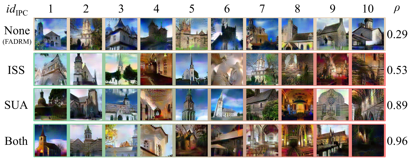
Figure 5 visualizes the effect of PSM on distilled data difficulty. Spearman’s $\rho$ (Spearman, 1904) measures agreement between the difficulty trends of distilled and original data, with values closer to 1 indicating stronger agreement. FADRM produces similar data difficulties and the lowest $\rho$ . Using ISS or SUA introduces clear difficulty variation, while combining both yields the clearest variation and the highest $\rho$ , confirming that PSM effectively captures the difficulty structure.

6 Conclusion

In this work, we identify that existing decoupled methods struggle to capture the difficulty variation in the original data fully. To address this issue, we propose Precise Statistical Matching (PSM) by Difficulty. We first introduce GPS to rank and group original data by difficulty using BN statistics. We then propose SUA to update teacher BN statistics through efficient forward propagation, enabling difficulty-specific statistical supervision. Meanwhile, ISS selects real samples from the corresponding difficulty groups for initialization, providing distilled data with starting points consistent with the target difficulty. Extensive experiments show that PSM consistently improves student performance and better preserves the difficulty distribution of the original data. Future work will further improve PSM under extreme settings (e.g., $\mathrm{IPC}=1$ ), and investigate the effects of its parameters on datasets with different distributions (e.g., fine-grained datasets).

References

Cai et al. (2026) W. Cai, Y. Zou, G. Li, C. Gu, and C. Zhang EVLF: early vision-language fusion for generative dataset distillation. In Proceedings of the IEEE/CVF Conference on Computer Vision and Pattern Recognition (CVPR), pp. 33953–33962. Cited by: Appendix A, §2.
Cazenavette et al. (2022) G. Cazenavette, T. Wang, A. Torralba, A. A. Efros, and J. Zhu Dataset distillation by matching training trajectories. In Proceedings of the IEEE/CVF Conference on Computer Vision and Pattern Recognition (CVPR), pp. 10718–10727. Cited by: §C.1.
Chen et al. (2023) M. Chen, B. Huang, J. Lu, B. Li, Y. Wang, M. Cheng, and W. Wang Dataset distillation via adversarial prediction matching. arXiv preprint arXiv:2312.08912. Cited by: Appendix A, §2.
Chen et al. (2025) Y. Chen, G. Chen, M. Zhang, W. Guan, and L. Nie Curriculum coarse-to-fine selection for high-ipc dataset distillation. In Proceedings of the Computer Vision and Pattern Recognition Conference (CVPR), pp. 20437–20446. Cited by: §5.3.
Chen et al. (2010) Y. Chen, M. Welling, and A. Smola Super-samples from kernel herding. In Proceedings of the Conference on Uncertainty in Artificial Intelligence (UAI), Cited by: §C.1.
Cui et al. (2025a) J. Cui, X. Bi, Y. Luo, X. Zhao, J. Liu, and Z. Shen FADRM: fast and accurate data residual matching for dataset distillation. In Proceedings of the Advances in Neural Information Processing Systems (NeurIPS), Cited by: Appendix A, Appendix A, §C.2, §5.1.
Cui et al. (2025b) J. Cui, Z. Li, X. Ma, X. Bi, Y. Luo, and Z. Shen Dataset distillation via committee voting. arXiv preprint arXiv:2501.07575. Cited by: Appendix A.
Cui et al. (2026) J. Cui, B. Tong, X. Bi, X. Zhao, J. Liu, and Z. Shen Hard labels in! rethinking the role of hard labels in mitigating local semantic drift. In Proceedings of the International Conference on Machine Learning (ICML), Cited by: §4.1.
Cui et al. (2023) J. Cui, R. Wang, S. Si, and C. Hsieh Scaling up dataset distillation to imagenet-1k with constant memory. In Proceedings of the International Conference on Machine Learning (ICML), pp. 6565–6590. Cited by: Appendix A, §C.1.
Deng et al. (2009) J. Deng, W. Dong, R. Socher, L. Li, K. Li, and L. Fei-Fei ImageNet: a large-scale hierarchical image database. In Proceedings of the IEEE Conference on Computer Vision and Pattern Recognition (CVPR), pp. 248–255. Cited by: §5.1.
Gan et al. (2026) Z. Gan, Q. Zhu, and L. Zhang Set-coupled guidance: set-level coordination in diffusion-based dataset distillation. In Proceedings of the International Conference on Machine Learning (ICML), Cited by: §1.
Gu et al. (2024) J. Gu, S. Vahidian, V. Kungurtsev, H. Wang, W. Jiang, Y. You, and Y. Chen Efficient dataset distillation via minimax diffusion. In Proceedings of the IEEE/CVF Conference on Computer Vision and Pattern Recognition (CVPR), pp. 15793–15803. Cited by: Appendix A, §C.1.
Guo et al. (2024) Z. Guo, K. Wang, G. Cazenavette, H. Li, K. Zhang, and Y. You Towards lossless dataset distillation via difficulty-aligned trajectory matching. In Proceedings of the International Conference on Learning Representations (ICLR), Cited by: Appendix A, §C.1, §2.
He et al. (2016) K. He, X. Zhang, S. Ren, and J. Sun Deep residual learning for image recognition. In Proceedings of the IEEE Conference on Computer Vision and Pattern Recognition (CVPR), pp. 770–778. Cited by: §5.1, Table 1.
Hoffmann et al. (2022) J. Hoffmann, S. Borgeaud, A. Mensch, E. Buchatskaya, T. Cai, E. Rutherford, D. de Las Casas, L. A. Hendricks, J. Welbl, A. Clark, T. Hennigan, E. Noland, K. Millican, G. v. d. Driessche, B. Damoc, A. Guy, S. Osindero, K. Simonyan, E. Elsen, J. W. Rae, O. Vinyals, and L. Sifre Training compute-optimal large language models. In Proceedings of the Advances in Neural Information Processing Systems (NeurIPS), Cited by: §1.
Huang et al. (2017) G. Huang, Z. Liu, L. Van Der Maaten, and K. Q. Weinberger Densely connected convolutional networks. In Proceedings of the IEEE Conference on Computer Vision and Pattern Recognition (CVPR), pp. 4700–4708. Cited by: §5.1.
Ioffe and Szegedy (2015) S. Ioffe and C. Szegedy Batch normalization: accelerating deep network training by reducing internal covariate shift. In Proceedings of the International Conference on Machine Learning (ICML), pp. 448–456. Cited by: Appendix A, §1, §3.3.
Ioffe (2017) S. Ioffe Batch renormalization: towards reducing minibatch dependence in batch-normalized models. In Proceedings of the Advances in Neural Information Processing Systems (NeurIPS), Cited by: Appendix A.
Krizhevsky (2009) A. Krizhevsky Learning multiple layers of features from tiny images. Technical report University of Toronto. Cited by: §5.1.
Le and Yang (2015) Y. Le and X. Yang Tiny imagenet visual recognition challenge. CS 231N 7 (7), pp. 3. Cited by: §5.1.
Lee et al. (2022) S. Lee, S. Chun, S. Jung, S. Yun, and S. Yoon Dataset condensation with contrastive signals. In Proceedings of the International Conference on Machine Learning (ICML), pp. 12352–12364. Cited by: Appendix A, §2.
Lee and Chung (2024) Y. Lee and H. W. Chung SelMatch: effectively scaling up dataset distillation via selection-based initialization and partial updates by trajectory matching. In Proceedings of the International Conference on Machine Learning (ICML), Cited by: §4.2.3.
Lei and Tao (2024) S. Lei and D. Tao A comprehensive survey of dataset distillation. IEEE Transactions on Pattern Analysis and Machine Intelligence 46 (1), pp. 17–32. Cited by: §1.
Li et al. (2020) G. Li, R. Togo, T. Ogawa, and M. Haseyama Soft-label anonymous gastric x-ray image distillation. In Proceedings of the IEEE International Conference on Image Processing (ICIP), pp. 305–309. Cited by: Appendix A.
Li et al. (2022a) G. Li, R. Togo, T. Ogawa, and M. Haseyama Compressed gastric image generation based on soft-label dataset distillation for medical data sharing. Computer Methods and Programs in Biomedicine 227, pp. 107189. Cited by: Appendix A.
Li et al. (2024a) G. Li, R. Togo, T. Ogawa, and M. Haseyama Dataset distillation using parameter pruning. IEICE Transactions on Fundamentals of Electronics, Communications and Computer Sciences 107 (6), pp. 936–940. Cited by: Appendix A.
Li et al. (2024b) G. Li, R. Togo, T. Ogawa, and M. Haseyama Importance-aware adaptive dataset distillation. Neural Networks 172, pp. 106154. Cited by: Appendix A.
Li et al. (2022b) G. Li, B. Zhao, and T. Wang Awesome dataset distillation. Note: https://github.com/Guang000/Awesome-Dataset-Distillation Cited by: Appendix A.
Li et al. (2025a) M. Li, G. Li, J. Mao, L. Ye, T. Ogawa, and M. Haseyama Task-specific generative dataset distillation with difficulty-guided sampling. In IEEE/CVF International Conference on Computer Vision (ICCV), Workshop, Cited by: Appendix A.
Li et al. (2025b) W. Li, G. Li, K. Maeda, T. Ogawa, and M. Haseyama Decoupled audio-visual dataset distillation. arXiv preprint arXiv:2511.17890. Cited by: Appendix A.
Li et al. (2025c) W. Li, G. Li, K. Maeda, T. Ogawa, and M. Haseyama Hyperbolic dataset distillation. In Proceedings of the Advances in Neural Information Processing Systems (NeurIPS), Cited by: §2.
Li et al. (2026) X. Li, Z. Luo, Z. Cui, and Z. Xu GeoDM: geometry-aware distribution matching for dataset distillation. In Proceedings of the International Conference on Machine Learning (ICML), Cited by: §1.
Li et al. (2017) Y. Li, N. Wang, J. Shi, J. Liu, and X. Hou Revisiting batch normalization for practical domain adaptation. In International Conference on Learning Representations (ICLR) Workshop, Cited by: Appendix A.
Liu and Du (2025) P. Liu and J. Du The evolution of dataset distillation: toward scalable and generalizable solutions. arXiv preprint arXiv:2502.05673. Cited by: §1.
Liu et al. (2023) Y. Liu, J. Gu, K. Wang, Z. Zhu, W. Jiang, and Y. You DREAM: efficient dataset distillation by representative matching. In Proceedings of the IEEE/CVF International Conference on Computer Vision (ICCV), pp. 17314–17324. Cited by: Appendix A, §2.
Luo et al. (2019) P. Luo, X. Wang, W. Shao, and Z. Peng Towards understanding regularization in batch normalization. In Proceedings of the International Conference on Learning Representations (ICLR), Cited by: Appendix A.
Ma et al. (2018) N. Ma, X. Zhang, H. Zheng, and J. Sun ShuffleNet v2: practical guidelines for efficient cnn architecture design. In Proceedings of the European Conference on Computer Vision (ECCV), pp. 116–131. Cited by: §5.1.
Peebles and Xie (2023) W. Peebles and S. Xie Scalable diffusion models with transformers. In Proceedings of the IEEE/CVF International Conference on Computer Vision (ICCV), pp. 4195–4205. Cited by: §C.1.
Sajedi et al. (2023) A. Sajedi, S. Khaki, E. Amjadian, L. Z. Liu, Y. A. Lawryshyn, and K. N. Plataniotis DataDAM: efficient dataset distillation with attention matching. In Proceedings of the IEEE/CVF International Conference on Computer Vision (ICCV), pp. 17097–17107. Cited by: Appendix A.
Sandler et al. (2018) M. Sandler, A. Howard, M. Zhu, A. Zhmoginov, and L. Chen Mobilenetv2: inverted residuals and linear bottlenecks. In Proceedings of the IEEE Conference on Computer Vision and Pattern Recognition (CVPR), pp. 4510–4520. Cited by: §5.1.
Sangermano et al. (2022) M. Sangermano, A. Carta, A. Cossu, and D. Bacciu Sample condensation in online continual learning. In Proceedings of the International Joint Conference on Neural Networks (IJCNN), pp. 1–8. Cited by: §1.
Santurkar et al. (2018) S. Santurkar, D. Tsipras, A. Ilyas, and A. Madry How does batch normalization help optimization?. In Proceedings of the Advances in Neural Information Processing Systems (NeurIPS), Cited by: Appendix A.
Shang et al. (2026) X. Shang, P. Sun, B. Shi, Z. Wang, and T. Lin Condensing large-scale datasets directly with minimal information loss. In Proceedings of the European Conference on Computer Vision (ECCV), Cited by: §1, §4.1.
Shao et al. (2024a) S. Shao, Z. Yin, M. Zhou, X. Zhang, and Z. Shen Generalized large-scale data condensation via various backbone and statistical matching. In Proceedings of the IEEE/CVF Conference on Computer Vision and Pattern Recognition (CVPR), pp. 16709–16718. Cited by: Appendix A.
Shao et al. (2024b) S. Shao, Z. Zhou, H. Chen, and Z. Shen Elucidating the design space of dataset condensation. In Proceedings of the Advances in Neural Information Processing Systems (NeurIPS), Cited by: Appendix A, §4.2.3.
Shi et al. (2026) G. Shi, X. Liang, and Q. Wen Balanced dataset distillation via modeling multiple visual pattern distribution. In Proceedings of the IEEE/CVF Conference on Computer Vision and Pattern Recognition (CVPR), pp. 19634–19643. Cited by: §4.1.
Spearman (1904) C. Spearman The proof and measurement of association between two things. The American Journal of Psychology 15 (1), pp. 72–101. External Links: Document Cited by: §5.4.
Su et al. (2024) D. Su, J. Hou, W. Gao, Y. Tian, and B. Tang D4M: dataset distillation via disentangled diffusion model. In Proceedings of the IEEE/CVF Conference on Computer Vision and Pattern Recognition (CVPR), pp. 5809–5818. Cited by: Appendix A.
Sun et al. (2024) P. Sun, B. Shi, D. Yu, and T. Lin On the diversity and realism of distilled dataset: an efficient dataset distillation paradigm. In Proceedings of the IEEE/CVF Conference on Computer Vision and Pattern Recognition (CVPR), pp. 9390–9399. Cited by: §5.1.
Swayamdipta et al. (2020) S. Swayamdipta, R. Schwartz, N. Lourie, Y. Wang, H. Hajishirzi, N. A. Smith, and Y. Choi Dataset cartography: mapping and diagnosing datasets with training dynamics. In Proceedings of the Conference on Empirical Methods in Natural Language Processing (EMNLP), pp. 9275–9293. Cited by: §5.3.
Toneva et al. (2019) M. Toneva, A. Sordoni, R. Tachet des Combes, A. Trischler, Y. Bengio, and G. J. Gordon An empirical study of example forgetting during deep neural network learning. In Proceedings of the International Conference on Learning Representations (ICLR), Cited by: §5.3.
Touvron et al. (2021) H. Touvron, M. Cord, M. Douze, F. Massa, A. Sablayrolles, and H. Jégou Training data-efficient image transformers & distillation through attention. In Proceedings of the International Conference on Machine Learning (ICML), pp. 10347–10357. Cited by: Table 3.
Vaswani et al. (2017) A. Vaswani, N. Shazeer, N. Parmar, J. Uszkoreit, L. Jones, A. N. Gomez, Ł. Kaiser, and I. Polosukhin Attention is all you need. In Proceedings of the Advances in Neural Information Processing Systems (NeurIPS), Cited by: Table 3.
Wang et al. (2022) K. Wang, B. Zhao, X. Peng, Z. Zhu, S. Yang, S. Wang, G. Huang, H. Bilen, X. Wang, and Y. You CAFE: learning to condense dataset by aligning features. In Proceedings of the IEEE/CVF Conference on Computer Vision and Pattern Recognition (CVPR), pp. 12196–12205. Cited by: Appendix A.
Wang et al. (2018) T. Wang, J. Zhu, A. Torralba, and A. A. Efros Dataset distillation. arXiv preprint arXiv:1811.10959. Cited by: Appendix A.
Xiao and He (2024) L. Xiao and Y. He Are large-scale soft labels necessary for large-scale dataset distillation?. In Proceedings of the Advances in Neural Information Processing Systems (NeurIPS), Cited by: Appendix A, §2.
Ye et al. (2025) L. Ye, S. M. Hamidi, G. Li, T. Ogawa, M. Haseyama, and K. N. Plataniotis Information-guided diffusion sampling for dataset distillation. In Advances in Neural Information Processing Systems (NeurIPS), Workshop, Cited by: Appendix A.
Yin and Shen (2024) Z. Yin and Z. Shen Dataset distillation in large data era. Transactions on Machine Learning Research. Cited by: Appendix A, Appendix A, §2.
Yin et al. (2023) Z. Yin, E. Xing, and Z. Shen Squeeze, recover and relabel: dataset condensation at imagenet scale from a new perspective. In Proceedings of the Advances in Neural Information Processing Systems (NeurIPS), Cited by: Appendix A, Appendix A, §1, §3.2, §4.1, §5.1.
Zhao and Bilen (2021) B. Zhao and H. Bilen Dataset condensation with differentiable siamese augmentation. In Proceedings of the International Conference on Machine Learning (ICML), pp. 12674–12685. Cited by: Appendix A, §C.1, §1.
Zhao and Bilen (2023) B. Zhao and H. Bilen Dataset condensation with distribution matching. In Proceedings of the IEEE/CVF Winter Conference on Applications of Computer Vision (WACV), pp. 6514–6523. Cited by: Appendix A, §C.1, §2.
Zhao et al. (2021) B. Zhao, K. R. Mopuri, and H. Bilen Dataset condensation with gradient matching. In Proceedings of the International Conference on Learning Representations (ICLR), Cited by: Appendix A.
Zhong et al. (2025a) W. Zhong, H. Tang, Q. Zheng, M. Xu, Y. Hu, and W. Guan Towards stable and storage-efficient dataset distillation: matching convexified trajectory. In Proceedings of the IEEE/CVF Conference on Computer Vision and Pattern Recognition (CVPR), Cited by: §1.
Zhong et al. (2025b) X. Zhong, H. Fang, B. Chen, X. Gu, M. Qiu, S. Qi, and S. Xia Hierarchical features matter: a deep exploration of progressive parameterization method for dataset distillation. In Proceedings of the Computer Vision and Pattern Recognition Conference (CVPR), pp. 30462–30471. Cited by: Appendix A, §2.
Zou et al. (2025) Y. Zou, G. Li, D. Su, Z. Wang, J. Yu, and C. Zhang Dataset distillation via vision-language category prototype. In Proceedings of the IEEE/CVF International Conference on Computer Vision (ICCV), pp. 2941–2950. Cited by: Appendix A.

Appendix A Additional Related Work

Dataset Distillation.

Dataset distillation (DD) (Wang et al., 2018; Li et al., 2022b) compresses a large dataset into a small set of samples with high training utility, substantially reducing storage and training costs while maintaining performance comparable to training on the full dataset (Li et al., 2020; Li et al., 2022a). Existing methods mainly include gradient matching (Zhao et al., 2021; Zhao and Bilen, 2021; Lee et al., 2022; Liu et al., 2023), distribution matching (Zhao and Bilen, 2023; Wang et al., 2022; Sajedi et al., 2023; Li et al., 2025b), trajectory matching (Cui et al., 2023; Chen et al., 2023; Guo et al., 2024; Li et al., 2024a; Li et al., 2024b), decoupled distillation (Yin et al., 2023; Cui et al., 2025a; Shao et al., 2024b; Yin and Shen, 2024), and generative distillation (Zhong et al., 2025b; Gu et al., 2024; Su et al., 2024; Li et al., 2025a; Ye et al., 2025; Zou et al., 2025; Cai et al., 2026).

Decoupled Dataset Distillation.

SRe²L (Yin et al., 2023) pioneered decoupled DD by separating teacher pretraining from distilled data optimization. SRe²L++ (Cui et al., 2025b) improves robustness through stronger data augmentation and soft labels specific to each batch. FADRM (Cui et al., 2025a) uses multiscale data residual connections to preserve original information and enrich distilled samples, while FADRM+ extends it to multiple teachers. G-VBSM (Shao et al., 2024a) employs lightweight model ensembles to improve generalization across architectures, while CDA (Yin and Shen, 2024) stabilizes optimization through a curriculum strategy. LPLD (Xiao and He, 2024) reexamines the need for large volumes of soft labels and provides a lighter alternative. Despite their strong performance on standard benchmarks, these methods do not explicitly consider the difficulty structure of the original data and its influence on distilled samples.

Batch Normalization.

Batch Normalization (BN) (Ioffe and Szegedy, 2015) normalizes intermediate features using batch means and variances, improving training speed and stability. Batch Renormalization (Ioffe, 2017) uses running statistics to reduce dependence on batch composition and improve training with small batches. Santurkar et al. (Santurkar et al., 2018) show that BN smooths the optimization landscape and stabilizes gradients. Luo et al. (Luo et al., 2019) interpret BN as implicit regularization and analyze its effects on convergence and generalization. AdaBN (Li et al., 2017) adapts BN statistics across domains, showing that they characterize domain distributions. Overall, BN improves training stability, while its running means and variances capture layer-wise feature distributions, supporting their use as statistical supervision in decoupled dataset distillation.

Appendix B Theoretical Analysis

B.1 The Empirical Relationship Between GPS and Classification Difficulty

GPS measures the distance between the statistics produced by a sample at the inputs to the teacher’s BN layers and the corresponding BN running statistics, thereby characterizing its deviation from the feature distribution learned by the teacher. To analyze the correlation between statistical deviation and classification difficulty, we measure sample difficulty using the teacher’s cross-entropy loss on the ground truth label. For a sample $(x_{i},y_{i})$ , its classification difficulty is defined as

\ell_{i}=\mathcal{L}_{\mathrm{CE}}\!\left(f_{\theta}(x_{i}),y_{i}\right)=-\log p_{\theta}(y_{i}\mid x_{i}),

(8)

where $p_{\theta}(y_{i}\mid x_{i})$ denotes the probability that the teacher assigns to the ground truth class $y_{i}$ . A larger $\ell_{i}$ indicates lower confidence in the ground truth class and thus greater classification difficulty.

We conduct this analysis on CIFAR-10/100 and ImageNette/Woof using a pretrained ResNet18 teacher to compute the GPS of each original sample. Suppose the dataset contains $N$ samples, and let $\pi$ denote the index sequence obtained by sorting them in ascending order of GPS:

\operatorname{GPS}\!\left(x_{\pi(1)}\right)\leq\operatorname{GPS}\!\left(x_{\pi(2)}\right)\leq\cdots\leq\operatorname{GPS}\!\left(x_{\pi(N)}\right).

(9)

We then compute the corresponding cross-entropy loss $\ell_{\pi(r)}$ for each ordered sample and examine how the classification loss changes along the GPS ranking. As shown in Figure 6, the cross-entropy loss generally increases with GPS, and samples with larger GPS values tend to exhibit higher classification losses. This empirical result indicates that the statistical deviation measured by GPS varies consistently with the classification difficulty perceived by the teacher, supporting the use of GPS to rank and group the original samples from easy to difficult.

B.2 The Expected Convergence of Statistics

Proof of Proposition 1.

Fix an arbitrary teacher $k$ and difficulty group $g$ . Let $\mathcal{B}_{t}$ denote the $t$ -th forward batch independently drawn from $\mathcal{T}_{g}$ , and let $\widehat{\bm{\tau}}_{k,g}^{(t)}$ denote the batch statistics induced by $\mathcal{B}_{t}$ at all BN layers. Since the teacher parameters are fixed and the forward batches are identically distributed, we have

\mathbb{E}\left[\widehat{\bm{\tau}}_{k,g}^{(t)}\right]=\bm{\tau}_{k,g}^{\star},\qquad\forall t.

(10)

Applying the BN update rule in equation 3 componentwise to all running means and variances gives

\bm{\tau}_{k,g}^{(t)}=(1-\rho)\bm{\tau}_{k,g}^{(t-1)}+\rho\widehat{\bm{\tau}}_{k,g}^{(t)},

(11)

where SUA starts from the global statistics stored in the pretrained teacher:

\bm{\tau}_{k,g}^{(0)}=\bm{\tau}_{k}^{\mathrm{G}}.

(12)

Taking expectations in equation 11 and using equation 10, we obtain

\displaystyle\mathbb{E}\left[\bm{\tau}_{k,g}^{(t)}\right]-\bm{\tau}_{k,g}^{\star}

\displaystyle=(1-\rho)\left(\mathbb{E}\left[\bm{\tau}_{k,g}^{(t-1)}\right]-\bm{\tau}_{k,g}^{\star}\right).

(13)

Recursively applying equation 13 and substituting equation 12 yields

\mathbb{E}\left[\bm{\tau}_{k,g}^{(t)}\right]-\bm{\tau}_{k,g}^{\star}=(1-\rho)^{t}\left(\bm{\tau}_{k}^{\mathrm{G}}-\bm{\tau}_{k,g}^{\star}\right).

(14)

Since $\rho\in(0,1]$ , we have $0\leq 1-\rho<1$ . Therefore,

\mathbb{E}\left[\bm{\tau}_{k,g}^{(t)}\right]-\bm{\tau}_{k,g}^{\star}\xrightarrow{t\rightarrow\infty}\bm{0}.

(15)

Thus, the expected discrepancy between the SUA running statistics and the statistics of the current difficulty group decreases geometrically with the number of forward batch updates. This result holds for the running means and variances of all BN layers. Consequently, SUA statistics converge in expectation to those of the current difficulty group and provide the corresponding statistical matching signal for distillation batch $g$ . ∎

Appendix C More Results

C.1 Comparison with other SOTA Methods

To further evaluate the effectiveness, we compare PSM with more representative SOTA dataset distillation methods, including the coreset selection methods Random and Herding (Chen et al., 2010), the gradient matching method DSA (Zhao and Bilen, 2021), the distribution matching method DM (Zhao and Bilen, 2023), the trajectory matching methods MTT (Cazenavette et al., 2022), DATM (Guo et al., 2024) and TESLA (Cui et al., 2023), the generative method Minimax (Gu et al., 2024), and the decoupled methods SRe²L and FADRM. Specifically, DSA uses ConvNet as the teacher model, DM uses ConvNet and ResNetAP-10, MTT uses ConvNet-BN, DATM and TESLA use ConvNet-IN, and Minimax uses DiT (Peebles and Xie, 2023), while SRe²L, FADRM, and PSM use ResNet18. All methods are evaluated using ResNet18 as the student model.

As shown in Table 6, coreset selection methods generally achieve lower accuracy, but gradually approach DD methods as IPC increases. For example, Random achieves $75.8\%$ on ImageNette with $\mathrm{IPC}=50$ . DD methods perform better in most settings, where gradient matching, distribution matching, trajectory matching, and generative methods use gradients, feature distributions, weight trajectories, and generative priors to guide distillation, respectively. Although these methods compress data effectively, their supervision signals usually describe the overall data distribution in an aggregated form, making it difficult to capture the internal difficulty structure. As dataset scale increases, sample difficulty differences are more easily smoothed by aggregated objectives, causing distilled data to concentrate at similar difficulties and limiting coverage of the original difficulty range. Among decoupled methods, FADRM performs strongly, while PSM preserves a broader difficulty structure, enabling students to learn sample patterns ranging from easy to difficult, and achieving the best results in most settings.

Table 6: Top-1 accuracy (%) comparison of representative dataset distillation methods with ResNet18 as the student. Standard deviations are reported when available.

Dataset	IPC	Coreset		Gradient	Distribution	Trajectory			Generative	Decoupled
Dataset	IPC	Random	Herding	DSA	DM	MTT	DATM	TESLA	Minimax	SRe²L	FADRM	PSM
CIFAR-10	1	–	–	–	–	–	–	–	–	$16.6_{\pm 0.9}$	$\underline{19.3}_{\pm 0.6}$	$\textbf{20.9}_{\pm 0.1}$
	10	$25.1_{\pm 0.5}$	$28.4_{\pm 0.1}$	$42.1_{\pm 0.6}$	$38.2_{\pm 1.1}$	$46.1_{\pm 1.4}$	48.66	$\underline{48.9}_{\pm 2.2}$	–	$29.3_{\pm 0.5}$	$48.2_{\pm 0.4}$	$\textbf{54.5}_{\pm 1.3}$
	50	54.96	–	$47.8_{\pm 0.9}$	$52.9_{\pm 0.4}$	$58.7_{\pm 0.2}$	66.27	–	–	$45.0_{\pm 0.7}$	$\underline{80.6}_{\pm 0.7}$	$\textbf{81.1}_{\pm 0.1}$
CIFAR-100	1	–	–	–	–	–	–	–	–	$6.6_{\pm 0.2}$	$\underline{31.3}_{\pm 0.2}$	$\textbf{32.9}_{\pm 0.9}$
	10	$10.9_{\pm 0.1}$	$13.3_{\pm 0.3}$	$21.9_{\pm 0.4}$	$18.7_{\pm 0.5}$	$26.8_{\pm 0.6}$	–	$27.1_{\pm 0.7}$	–	$27.0_{\pm 0.4}$	$\underline{64.7}_{\pm 0.4}$	$\textbf{66.7}_{\pm 0.4}$
	50	$40.7_{\pm 1.0}$	–	$43.6_{\pm 0.7}$	$42.6_{\pm 0.5}$	$51.3_{\pm 0.4}$	$51.0_{\pm 0.5}$	–	–	$50.2_{\pm 0.4}$	$\underline{69.3}_{\pm 0.3}$	$\textbf{69.7}_{\pm 0.3}$
ImageNette	1	–	–	–	–	–	–	–	–	$19.1_{\pm 1.1}$	$\textbf{28.2}_{\pm 0.6}$	$\underline{25.0}_{\pm 0.5}$
	10	$55.8_{\pm 1.0}$	–	–	$60.9_{\pm 0.7}$	–	–	–	$\underline{64.9}_{\pm 0.6}$	$29.4_{\pm 3.0}$	$64.0_{\pm 0.1}$	$\textbf{67.1}_{\pm 0.2}$
	50	$75.8_{\pm 1.1}$	–	–	$75.0_{\pm 1.0}$	–	–	–	$78.1_{\pm 0.6}$	$40.9_{\pm 0.3}$	$\underline{82.8}_{\pm 0.6}$	$\textbf{84.0}_{\pm 0.3}$
ImageWoof	1	–	–	–	–	–	–	–	–	$13.3_{\pm 0.5}$	$\underline{19.3}_{\pm 0.3}$	$\textbf{20.2}_{\pm 0.7}$
	10	$27.7_{\pm 0.9}$	$30.2_{\pm 1.2}$	–	$33.4_{\pm 0.7}$	–	–	–	$37.6_{\pm 0.9}$	$20.2_{\pm 0.2}$	$\underline{43.8}_{\pm 0.2}$	$\textbf{44.5}_{\pm 0.5}$
	50	$47.9_{\pm 1.8}$	$48.3_{\pm 1.2}$	–	$46.2_{\pm 0.6}$	–	–	–	$57.1_{\pm 0.6}$	$23.3_{\pm 0.3}$	$\underline{67.7}_{\pm 1.0}$	$\textbf{69.6}_{\pm 0.9}$
Tiny-ImageNet	1	–	–	–	–	–	–	–	–	$2.6_{\pm 0.1}$	$\underline{28.6}_{\pm 0.1}$	$\textbf{30.6}_{\pm 1.3}$
	10	$7.5_{\pm 0.1}$	$9.0_{\pm 0.3}$	–	–	–	–	–	–	$16.1_{\pm 0.2}$	$\underline{46.5}_{\pm 0.4}$	$\textbf{48.1}_{\pm 0.3}$
	50	$30.1_{\pm 0.6}$	–	$27.8_{\pm 1.4}$	$31.0_{\pm 0.6}$	$40.3_{\pm 0.3}$	$42.2_{\pm 0.2}$	–	–	$41.1_{\pm 0.4}$	$\underline{51.4}_{\pm 0.1}$	$\textbf{51.7}_{\pm 0.1}$
ImageNet-1K	10	$4.4_{\pm 0.1}$	$5.8_{\pm 0.1}$	–	–	–	–	$7.7_{\pm 0.1}$	$44.3_{\pm 0.5}$	$21.3_{\pm 0.6}$	$\underline{47.8}_{\pm 0.4}$	$\textbf{48.8}_{\pm 0.2}$
ImageNet-1K	50	–	–	–	–	–	–	–	$58.6_{\pm 0.3}$	$46.8_{\pm 0.2}$	$\underline{60.9}_{\pm 0.1}$	$\textbf{61.3}_{\pm 0.1}$

Epoch Ratio	DenseNet121	MobileNetV2	ShuffleNetV2	ResNet18
0.1	$68.6_{\pm 0.6}$	$51.5_{\pm 0.6}$	$49.1_{\pm 1.1}$	$65.5_{\pm 0.7}$
0.2	$68.8_{\pm 0.7}$	$51.8_{\pm 1.0}$	$\underline{50.2}_{\pm 2.5}$	$65.4_{\pm 0.4}$
0.3	$68.9_{\pm 1.0}$	$50.0_{\pm 0.7}$	$48.8_{\pm 0.1}$	$64.9_{\pm 0.7}$
0.4	$68.3_{\pm 0.9}$	$53.7_{\pm 1.1}$	$48.0_{\pm 2.1}$	$66.7_{\pm 0.7}$
0.5	$67.4_{\pm 1.1}$	$51.1_{\pm 0.5}$	$\textbf{50.3}_{\pm 1.3}$	$65.9_{\pm 0.4}$
0.6	$67.2_{\pm 0.2}$	$52.3_{\pm 0.8}$	$50.0_{\pm 1.5}$	$66.6_{\pm 0.7}$
0.7	$67.7_{\pm 1.2}$	$\textbf{54.2}_{\pm 0.7}$	$50.1_{\pm 1.6}$	$65.7_{\pm 1.1}$
0.8	$68.9_{\pm 0.3}$	$52.8_{\pm 1.5}$	$49.1_{\pm 0.8}$	$66.6_{\pm 0.2}$
0.9	$\underline{69.1}_{\pm 0.6}$	$\underline{53.9}_{\pm 3.4}$	$49.4_{\pm 1.3}$	$\underline{67.0}_{\pm 0.8}$
1.0	$\textbf{69.1}_{\pm 0.7}$	$52.0_{\pm 0.8}$	$49.5_{\pm 0.2}$	$\textbf{67.1}_{\pm 0.2}$

Table 7: Top-1 accuracy under different epoch ratios on ImageNette with

\mathrm{IPC}=10

under the same-architecture protocol.

Figure 7: Top-1 accuracy under different epoch ratios on Tiny-ImageNet and ImageNet-1K with

\mathrm{IPC}=10

and teacher=student=ResNet18.

C.2 More Ablation Study

Optimal Epoch Ratios for other Models.

To determine the optimal epoch ratio $r_{\mathrm{fwd}}$ for the other teacher models (DenseNet121, MobileNetV2, and ShuffleNetV2) in PSM+, we conduct an ablation study on ImageNette under the same-architecture protocol with $\mathrm{IPC}=10$ . As shown in Table 7, the optimal $r_{\mathrm{fwd}}$ values for DenseNet121, MobileNetV2, and ShuffleNetV2 are $1.0$ ( $69.1\%$ ), $0.7$ ( $54.2\%$ ), and $0.5$ ( $50.3\%$ ), respectively. Overall, models with more parameters require more forward passes to better capture the distribution of the current difficulty group. Since the performance gaps between the optimal $r_{\mathrm{fwd}}$ and $r_{\mathrm{fwd}}=1.0$ are small for MobileNetV2 and ShuffleNetV2, we apply the optimal $r_{\mathrm{fwd}}$ determined for ResNet18 to the other teacher models in PSM+ on other datasets and IPC settings for simplicity.

Epoch Ratio $r_{\mathrm{fwd}}$ on Tiny-ImageNet and ImageNet-1K.

Due to limited computational resources, we do not further investigate the effect of the ISS screening methods on Tiny-ImageNet and ImageNet-1K. Instead, we only examine the effect of different $r_{\mathrm{fwd}}$ under $\mathrm{IPC}=10$ , using ResNet18 as the teacher and student. As shown in Figure 7, consistent with the observations in Figure 4, larger $r_{\mathrm{fwd}}$ allows the statistics to better characterize the distribution of the current difficulty group. Both Tiny-ImageNet and ImageNet-1K achieve the highest accuracy at $r_{\mathrm{fwd}}=0.9$ , reaching $48.1\%$ and $48.8\%$ , respectively. Therefore, we set $r_{\mathrm{fwd}}=0.9$ for the other experiments on Tiny-ImageNet and ImageNet-1K.

Patch Grids in the Initial Image.

Since PSM modifies the sample initialization method, we further investigate the effect of different patch grids on performance. We use ResNet18 as the teacher and student with $\mathrm{IPC}=10$ , and the specific patch grid settings are illustrated in Figure 8. As shown in Table 8, the $1\times 1$ patch grid achieves the best performance on all datasets, consistent with the findings of (Cui et al., 2025a). When the patch grid increases to $2\times 2$ , compressing local image regions may cause information loss, which is more evident on high-resolution datasets. Therefore, we use the $1\times 1$ initialization setting in all experiments.

Patch Grid	CIFAR-10	CIFAR-100	ImageNette	ImageWoof
$1\times 1$	$54.5_{\pm 1.3}$	$66.7_{\pm 0.4}$	$67.1_{\pm 0.2}$	$44.5_{\pm 0.5}$
$2\times 2$	$54.3_{\pm 1.9}$	$65.0_{\pm 0.4}$	$65.1_{\pm 0.9}$	$40.2_{\pm 1.9}$

Table 9: Hyperparameter settings during pretraining and GPS.

Hyperparameter	CIFAR-10	CIFAR-100	Tiny-ImageNet	ImageNette	ImageWoof	ImageNet-1K
learning rate	$1.00\mathrm{E}{-03}$	$1.00\mathrm{E}{-03}$	$1.00\mathrm{E}{-02}$	$1.00\mathrm{E}{-02}$	$1.00\mathrm{E}{-02}$	PyTorch
optimizer	Adam	Adam	SGD	SGD	SGD
scheduler	cos	cos	cos	cos	cos
epoch	150	100	50	150	200	90
batch	512	512	128	64	64	64
$\beta$	1	1	1	1	1	1
$\epsilon$	$1.00\mathrm{E}{-06}$	$1.00\mathrm{E}{-06}$	$1.00\mathrm{E}{-06}$	$1.00\mathrm{E}{-06}$	$1.00\mathrm{E}{-06}$	$1.00\mathrm{E}{-06}$

Algorithm 1 Global Precision Score (GPS)

1: Original set

\mathcal{T}=\{(x_{i},y_{i})\}_{i=1}^{N}

; pretrained teachers

\{f_{\theta_{k}}\}_{k=1}^{K}

; repeated evaluations

R

2: for each teacher

k=1,\ldots,K

3: for

r=1,\ldots,R

4: for each sample

x_{i}\in\mathcal{T}

5: Forward

x_{i}

through

f_{\theta_{k}}

and compute its statistics at all BN layers

6: Compute

s_{i,k}^{(r)}

using the statistical distances in equation 4

7: end for

8: end for

s_{i,k}\leftarrow\frac{1}{R}\sum_{r=1}^{R}s_{i,k}^{(r)}

10: Rank

s_{i,k}

within each class:

r_{i,k}\leftarrow\operatorname{rank}_{c}(s_{i,k})

11: end for

12:

\operatorname{GPS}(x_{i})\leftarrow\frac{1}{K}\sum_{k=1}^{K}r_{i,k}

for each

x_{i}\in\mathcal{T}

13: return Class-wise GPS rankings from easy to hard

Appendix D Implementation Details

D.1 Pretraining.

As shown in Table 9, we report the pretraining hyperparameters for ShuffleNetV2, ResNet18, ResNet50, MobileNetV2, and DenseNet121 on each dataset. To ensure that all teacher models in PSM+ undergo the same number of forward passes under the same $r_{\mathrm{fwd}}$ , we use the same number of pretraining epochs and the same pretraining configuration for all models on each dataset. For ImageNet-1K, we directly use the official pretrained weights provided by PyTorch.

After pretraining the teacher models, we compute GPS. The batch size is kept the same as in pretraining, with $\beta=1.0$ and $\epsilon=1\times 10^{-6}$ . The detailed procedure is shown in Algorithm 1.

Table 10: Hyperparameter settings during distillation.

Hyperparameter	CIFAR-10	CIFAR-100	Tiny-ImageNet	ImageNette	ImageWoof	ImageNet-1K
Epoch ratio	0.9	0.9	0.9	1.0	0.4	0.9
Screening method	Back	Back	Back	Front	Back	Back
PSM+ teachers	ShuffleNetV2, MobileNetV2, DenseNet121, ResNet18

Algorithm 2 Precise Statistical Matching

1: Difficulty groups

\{\mathcal{T}_{g,c}\}

obtained by GPS; pretrained teachers

\{f_{\theta_{k}}\}_{k=1}^{K}

; forward ratio

r_{\mathrm{fwd}}

; pretraining epochs

\{E_{k}^{\mathrm{pre}}\}_{k=1}^{K}

; optimization iterations

T

2: Distilled dataset

\widetilde{\mathcal{T}}

3: Initialize

\widetilde{\mathcal{T}}\leftarrow\varnothing

4: for

g=1,\ldots,\mathrm{IPC}

5: SUA: construct difficulty-specific statistical supervision

6: for each teacher

k=1,\ldots,K

7: Freeze

\theta_{k}

and initialize BN statistics with

\bm{\tau}_{k}^{\mathrm{G}}

8: Forward

\mathcal{T}_{g}=\bigcup_{c}\mathcal{T}_{g,c}

through

f_{\theta_{k}}

for

\left\lfloor r_{\mathrm{fwd}}E_{k}^{\mathrm{pre}}\right\rfloor

epochs

9: Update only BN running statistics according to equation 3

10: Store the updated statistics as

\bm{\tau}_{k,g}^{\mathrm{SUA}}

11: end for

12: ISS: initialize distilled data with matched difficulty

13: for each class

c

14: Select real samples from

\mathcal{T}_{g,c}

using ISS

15: Initialize

\widetilde{x}_{g,c}^{(0)}

with the selected samples

16: end for

17: Distillation:

18: for

t=1,\ldots,T

19: Select teacher

k

and use

\bm{\tau}_{k,g}^{\mathrm{SUA}}

as its statistical target

20: Update

\widetilde{\mathcal{T}}_{g}

by minimizing equation 2 with the SUA statistics

21: end for

22:

\widetilde{\mathcal{T}}\leftarrow\widetilde{\mathcal{T}}\cup\widetilde{\mathcal{T}}_{g}

23: end for

24: return

\widetilde{\mathcal{T}}

D.2 Distillation.

For PSM+, to simplify the experimental setup, we use ShuffleNetV2, ResNet18, MobileNetV2, and DenseNet121 as teacher models on all datasets, while using the same teacher model settings as FADRM+. During the forward passes of SUA, the batch size fed into the teacher models is kept the same as that used during pretraining to reduce statistical bias. The remaining hyperparameters are shown in Table 10, and the detailed procedure is provided in Algorithm 2. It is worth noting that when $\mathrm{IPC}=1$ , there is only one difficulty group, meaning that the entire dataset is treated as a single group. In this case, only ISS takes effect in PSM. Therefore, as shown in Table 1, PSM and FADRM(+) achieve similar performance on most datasets when $\mathrm{IPC}=1$ .

D.3 Soft Label Generation.

To maintain consistency in the soft label distribution, we use the original pretrained teachers to generate soft labels, rather than the teachers after forward passes. For FADRM+ and PSM+, we assign equal weights to all teachers during soft label generation to simplify the experimental setup.

Appendix E More Visualization

To more intuitively illustrate the changes in the difficulty of distilled samples, we visualize the samples generated by FADRM and PSM with ResNet18 as the teacher model and $\mathrm{IPC}=10$ . Due to space limitations, we only show results on CIFAR-10, ImageNette, and ImageWoof.

As shown in Figure 9, 11 and 13, the distilled samples generated by FADRM are typically concentrated within a relatively narrow difficulty range. In contrast, as shown in Figure 10, 12 and 14, PSM generates distilled samples that cover a broader difficulty range, promoting the student model to learn a more complete difficulty structure.

PSM: Dataset Distillation Based on Precise Statistical Matching by Difficulty

Abstract

1 Introduction

2 Related Work

3 Preliminaries

3.1 Dataset Distillation

3.2 Decoupled Dataset Distillation

I. Teacher model pretraining.

II. Distillation.

III. Soft label generation.

3.3 Batch Normalization

4 Method

4.1 Limitations of Decoupled Dataset Distillation

Homogeneous Supervision.

4.2 Dataset Distillation Based on Precise Statistical Matching by Difficulty

4.2.1 GPS: Global Precision Score

Operation and Purpose.

Empirical Observation.

4.2.2 SUA: Statistics Updated Again

Operation and Purpose.

Proposition 1 (Expected Convergence; Proof in Appendix B.2).

4.2.3 ISS: Initial Sample Screening

5 Experiments

5.1 Experimental Setup

Baselines.

Datasets.

Implementation Details.

5.2 Comparison With State-of-The-Art Methods

5.2.1 Main Results

Low-resolution datasets.

High-resolution datasets.

5.2.2 Difficulty and Efficiency Analysis.

Difficulty.

Efficiency.

5.2.3 Cross-architecture Generalization.

Small-scale datasets.

Large-scale datasets.

5.3 Ablation Study

Difficulty Calculation Methods.

Epoch Ratio in SUA and Screening Method in ISS.

Ablation of Mechanisms.

5.4 Visualization

6 Conclusion

References

Appendix A Additional Related Work

Dataset Distillation.

Decoupled Dataset Distillation.

Batch Normalization.

Appendix B Theoretical Analysis

B.1 The Empirical Relationship Between GPS and Classification Difficulty

B.2 The Expected Convergence of Statistics

Proof of Proposition 1.

Appendix C More Results

C.1 Comparison with other SOTA Methods

C.2 More Ablation Study

Optimal Epoch Ratios for other Models.

Epoch Ratio rfwdr_{\mathrm{fwd}} on Tiny-ImageNet and ImageNet-1K.

Patch Grids in the Initial Image.

Appendix D Implementation Details

D.1 Pretraining.

D.2 Distillation.

D.3 Soft Label Generation.

Appendix E More Visualization

Epoch Ratio $r_{\mathrm{fwd}}$ on Tiny-ImageNet and ImageNet-1K.