Cardinality-Stratified Interaction Decomposition for Interpretable Pairwise and Higher-Order Structure in Transactional Basket Data

Let $V=\{1,\ldots,N\}$ be the item set and let

$$x=(x_{1},\ldots,x_{N})\in\{0,1\}^{N}$$

(1)

represent one basket, with $x_{i}=1$ if item $i$ is present. The basket cardinality is $|x|=\sum_{i}x_{i}$.

The ordinary $0/1$ pairwise Ising model is

$$P_{\mathrm{Ising}}(x)\propto\exp\left\{\sum_{i}h_{i}x_{i}+\sum_{i<j}J_{ij}x_{i}x_{j}\right\}.$$

(2)

To represent item-label-invariant basket-size structure, we first consider the cardinality-aware pairwise model

$$P(x)\propto\exp\left\{\alpha_{|x|}+\sum_{i}h_{i}x_{i}+\sum_{i<j}J_{ij}x_{i}x_{j}\right\}.$$

(3)

Here $\alpha_{|x|}$ captures single-item, small-basket, and large-basket tendencies, while $J_{ij}$ represents a pair-specific deviation from this common structure.

For a higher-order formulation, define $x_{U}=\prod_{i\in U}x_{i}$ for $U\subseteq V$ and consider the cardinality-aware log-linear model of maximum order $K$,

$$P(x)\propto\exp\left\{\alpha_{|x|}+\sum_{\begin{subarray}{c}\varnothing\neq U\subseteq V\\ |U|\leq K\end{subarray}}\theta_{U}x_{U}\right\}.$$

(4)

The singleton parameter is $\theta_{\{i\}}=h_{i}$, the pair parameter is $\theta_{\{i,j\}}=J_{ij}$, and $\theta_{U}$ for $|U|\geq 3$ is a higher-order interaction. The case $K=2$ is the cardinality-aware Ising model above.

For every order $k$,

$$\sum_{|S|=k}x_{S}=\binom{|x|}{k}.$$

(5)

When all order-$k$ subsets are included in eq. 4, the transformation

$$\theta_{S}\mapsto\theta_{S}+c\quad(|S|=k),\qquad\alpha_{m}\mapsto\alpha_{m}-c\binom{m}{k}$$

(6)

leaves the exponent, and hence the distribution, unchanged. This is the structural gauge freedom between the order-$k$ interaction block and the cardinality potential. When only a restricted family of order-$k$ subsets is included, however, their presence indicators need not sum to a function of $|x|$ alone, so this transformation does not generally preserve the distribution.

Let $T\subseteq V$ with $|T|=k$. Write $y=x_{-T}$ for the configuration outside $T$, and let $r=|y|$. For $A\subseteq T$, write $x_{T}=\mathbf{1}_{A}$ for the state in which exactly the items in $A$ are present within $T$. We define the order-$k$ log-odds contrast at fixed $y$ as

$$\Lambda_{T}(y)=\sum_{A\subseteq T}(-1)^{k-|A|}\log P(x_{T}=\mathbf{1}_{A},x_{-T}=y).$$

(7)

Substituting eq. 4 into eq. 7 gives the decomposition directly. The normalizing constant cancels because

$$\sum_{A\subseteq T}(-1)^{k-|A|}=0.$$

(8)

For an interaction monomial $x_{U}$, only interactions whose index set contains all elements of $T$ survive the contrast. Writing each surviving index set uniquely as $U=T\cup W$, with $W\subseteq\operatorname{supp}(y)$, the total interaction contribution to the contrast is

$$\sum_{\begin{subarray}{c}W\subseteq\operatorname{supp}(y)\\ |T|+|W|\leq K\end{subarray}}\theta_{T\cup W},$$

(9)

where

$$\operatorname{supp}(y)=\{i\in V\setminus T:y_{i}=1\}.$$

(10)

The cardinality term contributes

$$\sum_{A\subseteq T}(-1)^{k-|A|}\alpha_{|y|+|A|}=\sum_{\ell=0}^{k}(-1)^{k-\ell}\binom{k}{\ell}\alpha_{|y|+\ell}.$$

(11)

Therefore,

$$\Lambda_{T}(y)=\sum_{\begin{subarray}{c}W\subseteq\operatorname{supp}(y)\\ |T|+|W|\leq K\end{subarray}}\theta_{T\cup W}+\Delta^{k}\alpha_{|y|},$$

(12)

where

$$\Delta^{k}\alpha_{r}=\sum_{\ell=0}^{k}(-1)^{k-\ell}\binom{k}{\ell}\alpha_{r+\ell}.$$

(13)

In particular, when the maximum interaction order is $K=k$,

$$\Lambda_{T}(y)=\theta_{T}+\Delta^{k}\alpha_{|y|}.$$

(14)

For $k=2$, write $p_{ab}(y)=P(x_{i}=a,x_{j}=b,y)$. Then $\Lambda_{ij}(y)$ is the usual conditional pair log-odds ratio:

	$\displaystyle\Lambda_{ij}(y)$	$\displaystyle=\log\frac{p_{11}(y)p_{00}(y)}{p_{10}(y)p_{01}(y)}$		(15)
		$\displaystyle\equiv\log OR_{ij\mid y}.$

For $k=3$, $T=\{i,j,\ell\}$,

$$\Lambda_{ij\ell}(y)=\log OR_{ij\mid x_{\ell}=1,y}-\log OR_{ij\mid x_{\ell}=0,y}.$$

(16)

Thus, the sign of $\Lambda_{ij\ell}(y)$ indicates whether the conditional association between $i$ and $j$ is stronger or weaker when item $\ell$ is present. When $K=3$, the coefficient $\theta_{ij\ell}$ is the item-set-specific component of this change after removing the common cardinality contribution $\Delta^{3}\alpha_{|y|}$. A positive $\theta_{ij\ell}$ represents reinforcement beyond the common cardinality effect, whereas a negative value represents weakening or saturation. If $K>3$, eq. 12 shows that the contrast also contains higher-order interactions involving all three focal items.

Conditioning on every full rest vector $y$ rapidly produces sparse cells. We therefore stratify only by

$$R_{T}=|x_{-T}|.$$

(17)

For $A\subseteq T$, define

$$p_{T,r}^{A}=P(x_{T}=\mathbf{1}_{A},R_{T}=r)$$

(18)

and

$$\Lambda_{T,r}=\sum_{A\subseteq T}(-1)^{k-|A|}\log p_{T,r}^{A}.$$

(19)

Marginalizing the identities of rest items generally produces

$$\Lambda_{T,r}=\theta_{T}+\beta_{k,r}+\rho_{T,r},$$

(20)

where $\beta_{k,r}$ is common to order $k$ and rest cardinality $r$, while $\rho_{T,r}$ contains mediation and mixing effects induced by marginalization. We therefore target the additive projection

$$\Lambda_{T,r}\approx\theta_{T}+\beta_{k,r}.$$

(21)

When rest configurations are fully resolved, eq. 14 expresses the contrast through the model interaction $\theta_{T}$ at fixed $y$. Rest-cardinality stratification instead uses the additive summary eq. 21, in which $\theta_{T}$ denotes the item-set-specific component relative to the common order-$k$ environment.

The finite-sample estimator uses the corresponding gauge constraint. Let $g_{T}>0$ denote fixed reference weights used to select one representative from the equivalence class described above. A natural default is $g_{T}=\mu_{T}$, using the information weights in eq. 30. We impose

$$\sum_{T\in\mathcal{T}_{k}}g_{T}\theta_{T}=0.$$

(31)

When $\mathcal{T}_{k}$ is restricted, eq. 31 should be understood as a reference-weighted centering convention within the candidate family. Hence, within the chosen candidate family, the sign of $\widehat{\theta}_{\{i,j\}}$ indicates whether the pair-specific projection is stronger or weaker than the reference-weighted average pair under the same rest-cardinality environment.

To estimate eq. 21, we define CSID-$k$ as

$$(\widehat{\theta},\widehat{\beta})=\operatorname*{arg\,min}_{\theta,\beta}\left\{\frac{1}{2}\sum_{T\in\mathcal{T}_{k}}\sum_{r}w_{T,r}(\widehat{\Lambda}_{T,r}-\theta_{T}-\beta_{k,r})^{2}+\frac{\lambda_{k}}{2}\sum_{T\in\mathcal{T}_{k}}\theta_{T}^{2}\right\},$$

(32)

subject to the gauge constraint eq. 31. Dividing eq. 32 by $M$ makes its relation to eq. 25 explicit: $w_{T,r}/M\to q_{T,r}$ and $\widehat{\Lambda}_{T,r}\to\Lambda_{T,r}$. Hence, for fixed $\varepsilon$ and a fixed candidate family, the empirical minimizer converges to the population projection provided that the gauge-constrained population projection is uniquely identified, the normalized gauge weights converge to $\bar{g}_{T}^{\star}$, and the ridge parameter $\lambda_{k,M}$ at sample size $M$ satisfies $\lambda_{k,M}/M\to 0$ [31]. For the default $g_{T}=\mu_{T}$, the limiting normalized gauge weight is $\bar{g}_{T}^{\star}=(\sum_{r}q_{T,r})/(\sum_{U\in\mathcal{T}_{k}}\sum_{r}q_{U,r})$.

For finite $M$, $\lambda_{k}>0$ ensures a unique gauge-fixed $\theta$ block and unique $\beta_{k,r}$ for strata with $\sum_{T}w_{T,r}>0$. Zero-information strata are fixed to zero by convention. The resulting $\widehat{\theta}_{T}$ therefore depends on the candidate family, information weights, gauge, and ridge penalty.

Initialize $\beta_{k,r}^{(0)}=0$ and define at iteration $t$

$$S_{T}^{(t)}=\sum_{r}w_{T,r}(\widehat{\Lambda}_{T,r}-\beta_{k,r}^{(t)}).$$

(33)

The Lagrange multiplier for the gauge constraint is

$$\gamma^{(t)}=\frac{\displaystyle\sum_{T\in\mathcal{T}_{k}}\frac{g_{T}S_{T}^{(t)}}{\mu_{T}+\lambda_{k}}}{\displaystyle\sum_{T\in\mathcal{T}_{k}}\frac{g_{T}^{2}}{\mu_{T}+\lambda_{k}}},$$

(34)

and the exact update of the item-set block is

$$\theta_{T}^{(t+1)}=\frac{S_{T}^{(t)}-\gamma^{(t)}g_{T}}{\mu_{T}+\lambda_{k}}.$$

(35)

The rest-cardinality-common block is then updated by

$$\beta_{k,r}^{(t+1)}=\frac{\displaystyle\sum_{T\in\mathcal{T}_{k}}w_{T,r}(\widehat{\Lambda}_{T,r}-\theta_{T}^{(t+1)})}{\displaystyle\sum_{T\in\mathcal{T}_{k}}w_{T,r}}.$$

(36)

Unobserved $(T,r)$ cells are omitted by setting $w_{T,r}=0$. Each step exactly minimizes one block, so the objective decreases monotonically and converges to the unique optimum for $\theta$ and the informative $\beta$ strata under the stated convention.

To prioritize candidate item sets for subsequent analysis, we normalize each estimated component by its approximate estimation scale. Using the diagonal curvature $\lambda_{k}+\mu_{T}$ of eq. 32 as an information approximation gives

$$\widehat{s}_{T}=(\lambda_{k}+\mu_{T})^{-1/2},\qquad z_{T}=\frac{\widehat{\theta}_{T}}{\widehat{s}_{T}}.$$

(37)

Because this diagonal-curvature scale ignores uncertainty in the common effects, candidate overlap, and data-dependent screening, we use $|z_{T}|$ only as an information-normalized screening score, not for formal inference.

Under eq. 4 with $K=3$, applying eq. 12 to the pair $T=\{i,j\}$ gives

$$\Lambda_{ij}(y)=J_{ij}+\sum_{\ell\in\operatorname{supp}(y)}\theta_{ij\ell}+\Delta^{2}\alpha_{|y|}.$$

(38)

A pairwise estimate that ignores triples therefore absorbs all third-order terms containing the pair $(i,j)$.

At a fixed rest configuration $y$, define

$$g_{ij}(y)=\sum_{\ell\in\operatorname{supp}(y)}\theta_{ij\ell}.$$

(39)

Under eq. 38, all third-order terms containing both $i$ and $j$ enter only the $11$ cell, through $x_{i}x_{j}g_{ij}(y)$. If the true third-order coefficients are known, reweighting the four pair cells according to

$$\widetilde{P}_{ij,y}(a,b)\propto P(x_{i}=a,x_{j}=b,y)\exp\{-ab\,g_{ij}(y)\}$$

(40)

multiplies the $11$-cell mass by $\exp\{-g_{ij}(y)\}$ while leaving the other three cell masses unchanged before jointly normalizing all four cells. Let $\widetilde{\Lambda}_{ij}(y)$ denote the order-$2$ contrast eq. 7 for $T=\{i,j\}$, evaluated from the cell probabilities $\widetilde{P}_{ij,y}(a,b)$. Then

$$\widetilde{\Lambda}_{ij}(y)=J_{ij}+\Delta^{2}\alpha_{|y|}.$$

(41)

Thus the third-order contribution is removed exactly at fixed $y$.

The empirical analogue applies the same basket-level weighting with estimated coefficients and rest-cardinality aggregation. Using CSID-3, define the estimated third-order contribution associated with pair $(i,j)$ in basket $x$ as

$$\widehat{g}_{ij}(x)=\sum_{\ell:\{i,j,\ell\}\in\mathcal{T}_{3}}\widehat{\theta}_{ij\ell}x_{\ell}.$$

(42)

For $T=\{i,j\}$, $a,b\in\{0,1\}$, and rest cardinality $r$, we reconstruct the pairwise cell counts as

$$\widetilde{n}_{ij,r}^{ab}=\sum_{n:\,x_{i}^{(n)}=a,\,x_{j}^{(n)}=b,\,R_{T}^{(n)}=r}\exp\{-ab\,\widehat{g}_{ij}(x^{(n)})\}.$$

(43)

Only the $11$ cell is reweighted. Each observed basket receives the same basket-level weight $\exp\{-ab\,\widehat{g}_{ij}(x^{(n)})\}$ as in eq. 40, but the sum aggregates over all rest configurations with common cardinality $r$ rather than over a single $y$. Because baskets with the same $r$ can carry different weights when their rest configurations differ, $\widetilde{n}_{ij,r}^{ab}$ does not correspond to cell probabilities at any fixed $y$; it is a cardinality-stratified pseudo-count table. Replacing the structural coefficients by CSID-3 estimates adds a second approximation. Fitting CSID-2 to the reweighted counts yields a reweighted CSID-2 pairwise estimate. The reweighting is local to each pair, does not define one common joint distribution, and is therefore an approximate pair-specific deprojection in empirical data rather than an exact recovery of a global pairwise model.

We generated 10,000 baskets from a 10-item model with all true pairwise interactions fixed at $J_{ij}=0$. For each replicate, fields were sampled as $h_{i}\sim N(-0.30,0.25^{2})$ and the cardinality potential was

$$\alpha_{m}(s)=-s(m-1)^{1.3},\qquad m\geq 1.$$

(44)

We varied $s\in\{0,0.25,0.5,0.75,1.0\}$ and used 20 replicates per setting, holding $h_{i}$ fixed within each replicate so that only the cardinality potential changed.

Each sample was fitted with an ordinary pairwise Ising model without a cardinality term by exact maximum likelihood on the nonempty state space. A ridge penalty of $10^{-5}$ was used for numerical stability. CSID-2 was applied to the same sample with the settings reported above. The penalties serve different numerical roles and are not calibrated to be directly comparable; this experiment tests directional contamination caused by omitting the cardinality term, rather than general predictive superiority of one estimator.

Tables 1 and 1 summarize the results. When $s=0$, both methods were centered near zero. As the cardinality constraint strengthened, ordinary Ising couplings shifted systematically downward; 99.7% of fitted Ising pairs were negative at $s=0.5$, and every fitted pair was negative for $s\geq 0.75$, whereas CSID-2 retained a sign split near 50% negative and much smaller RMSE. The optimizer reported convergence for 98 of the 100 ordinary-Ising fits; retaining the two flagged fits does not affect the directional pattern. Thus an ordinary pairwise Ising model without a cardinality term can create apparently competitive edges even when no true pair-specific competition exists under this data-generating process.

For each replicate, we generated a new background with fields $h_{i}\sim N(-0.25,0.35^{2})$, independently retained 35% of pair coefficients with nonzero values drawn from $N(0,0.30^{2})$, and sampled the cardinality-strength parameter uniformly from $[0.50,0.80]$. We used ten items and 10,000 baskets. These settings were chosen to generate heterogeneous but nondegenerate pairwise and basket-cardinality structure rather than to match a particular empirical dataset. Eight of the $\binom{10}{3}=120$ triples were sampled uniformly, with four positive and four negative coefficients. Absolute effect sizes were $0.1$, $0.2$, $0.3$, and $0.5$, with 20 replicates per effect size. CSID-3 was fitted to all 120 triples, and screening performance was assessed with the score $z_{T}$ in (37). We treated $|z_{T}|\geq 2$ as a detection event; power and the non-planted exceedance rate count such events among planted and non-planted triples, respectively. Although non-planted triples have zero generating third-order coefficients, their marginalized CSID contrasts need not be zero because marginalizing over the identities of rest items can transmit association from planted triples. The non-planted exceedance rate therefore measures how often screening flags triples without a directly planted coefficient; it is not a type-I error rate under a global null of zero target contrasts. We also report AUPRC, AUROC, and sign recovery, noting that precision-recall and ROC summaries respond differently to class imbalance [33].

Tables 2 and 2 show that non-planted triples were rarely flagged and that this rate was stable across planted effect sizes. Detection rose with $|\theta|$: weak planted coefficients were usually missed, whereas strong ones were detected substantially more often and typically with the correct sign. The screening procedure is therefore conservative at this sample size, and is suitable for prioritizing candidates rather than exhaustively finding weak interactions.

We sampled 60,000 baskets from a 6-item model with

$$J_{AB}=J_{AC}=J_{BC}=0.8,\qquad\theta_{ABC}=-1.2,$$

(45)

and background interactions $J_{DE}=0.5$ and $J_{EF}=0.3$, together with a cardinality potential. Items $A,B,C$ are positively associated in pairs, but the negative triple coefficient induces saturation when all three are present. A pairwise projection that omits the triple therefore underestimates the generating pair coefficients.

To evaluate recovery, we compared standard CSID-2 with reweighted CSID-2 from the local deprojection procedure (eqs. 42 and 43). For gauge alignment, the information-weighted mean of the generating pair vector, using the fitted CSID-2 weights $\mu_{T}$, was subtracted from every generating pair coefficient before RMSE and correlation were computed (eq. 31).

Table 3 shows that reweighted CSID-2 tracks the generating pair coefficients substantially more closely than CSID-2 alone. In this controlled realization with known ground truth, the result demonstrates the underestimation expected when a triple is omitted from a pairwise projection (eq. 38).

Three public transaction datasets were each restricted to 20 selected categories for analysis (Table 4). The Complete Journey data were obtained through the completejourney package [34]; transactions were joined to products.csv, and a predefined list of 20 product_category values was retained from the full category catalog. The Ta-Feng data were originally described by Hsu et al. [35] and obtained from a Kaggle distribution [36]; SKUs were aggregated to the first two digits of PRODUCT_SUBCLASS, and the 20 codes with highest basket support over the full observation window were selected (minimum support 1,000). The Instacart data came from the 2017 public release [37], obtained from a Kaggle distribution [38]; 30,000 users were sampled from prior orders, products were aggregated to aisles, and the 20 aisles with highest order support were selected. In all cases, category presence was binarized within each basket and baskets with fewer than two selected categories were excluded. Temporal splits assign weeks 1–26 to H1 and week 27 onward to H2 in Complete Journey, November–December 2000 to H1 and January–February 2001 to H2 in Ta-Feng, and a user’s first ten orders to H1 and later orders to H2 in Instacart. Category universes were selected before the temporal split and then held fixed in both periods. All real-data fits used $\varepsilon=0.5$, $\lambda_{2}=\lambda_{3}=1$, and rest-cardinality strata $r\geq 2$. Candidates were enumerated exhaustively and filtered by the triple-count thresholds in table 4; the H1-retained candidate set was then fixed for H2 evaluation. H2 and the full-period evaluation reference were fitted on this same candidate family using $g_{T}=\mu_{T}^{\mathrm{H1}}$ in eq. 31, placing all period-comparison coefficients in a common gauge while retaining each fit’s own $\mu_{T}$ in eqs. 34 and 35.

Table 4 reports sample sizes, temporal splits, category definitions, and the $n_{111}$ minimum-count thresholds after this restriction. With 20 selected categories per dataset, CSID enumerates 190 pair candidates and up to 1,140 triple candidates exhaustively. Ta-Feng retains 1,066 triples in the full-sample fit and 1,001 H1-supported triples for H2 evaluation.

We first fitted CSID-3 separately in H1 and H2, with the H2 candidate family and gauge fixed from H1 as described above. Among common triple candidates, we ranked $\min(\mu_{T}^{\mathrm{H1}},\mu_{T}^{\mathrm{H2}})$ and evaluated the top information quartile using Pearson correlation, sign agreement, and overlap between the 20 most negative CSID-3 coefficients in H1 and H2. Sensitivity to shared categories was assessed by removing, one at a time, all evaluated triples containing a category without refitting the models (leave-one-category-out evaluation, LOCO).

Table 5 shows positive temporal correlation in all three datasets, directionally consistent descriptive LOCO ranges, and overlap among the 20 most negative third-order coefficients that exceeded random expectation.

We next assessed whether H1 effects reconstruct H2 stratified third-order contrasts. For triple $T=\{i,j,\ell\}$ and rest-cardinality stratum $r$, we built the eight H2 cells and computed

$$\widehat{\Lambda}_{T,r}^{\mathrm{H2}}=\sum_{A\subseteq T}(-1)^{3-|A|}\log(n_{T,r}^{A,\mathrm{H2}}+\varepsilon).$$

(46)

Equivalently,

$$\widehat{\Lambda}_{ij\ell,r}^{\mathrm{H2}}=\log\widehat{OR}_{ij\mid x_{\ell}=1,R_{T}=r}^{\mathrm{H2}}-\log\widehat{OR}_{ij\mid x_{\ell}=0,R_{T}=r}^{\mathrm{H2}}.$$

(47)

This quantity is computed only from H2 cells; it contains neither H1 estimates nor fitted values from eq. 32.

The projection eq. 21 motivates two reconstructions. Without a triple-specific component, estimate the H2 component common to rest cardinality $r$ from all triples other than $T$,

$$\widehat{\beta}_{3,r}^{\mathrm{H2},(-T)}=\frac{\sum_{U\neq T}w_{U,r}^{\mathrm{H2}}\widehat{\Lambda}_{U,r}^{\mathrm{H2}}}{\sum_{U\neq T}w_{U,r}^{\mathrm{H2}}},\qquad\widehat{\Lambda}_{T,r}^{\mathrm{base}}=\widehat{\beta}_{3,r}^{\mathrm{H2},(-T)}.$$

(48)

For CSID-3 transfer, rewrite eq. 21 as

$$\beta_{3,r}\approx\Lambda_{U,r}-\theta_{U}.$$

(49)

Remove the H1 triple-specific effect from the other H2 contrasts,

$$\widehat{\beta}_{3,r}^{\mathrm{H2}\mid\mathrm{H1},(-T)}=\frac{\sum_{U\neq T}w_{U,r}^{\mathrm{H2}}(\widehat{\Lambda}_{U,r}^{\mathrm{H2}}-\widehat{\theta}_{U}^{\mathrm{H1}})}{\sum_{U\neq T}w_{U,r}^{\mathrm{H2}}},$$

(50)

and add the H1 effect of the target triple,

$$\widehat{\Lambda}_{T,r}^{\mathrm{CSID3}}=\widehat{\beta}_{3,r}^{\mathrm{H2}\mid\mathrm{H1},(-T)}+\widehat{\theta}_{T}^{\mathrm{H1}}.$$

(51)

The subtraction in eq. 50 extracts the H2 rest-cardinality-common component after removing other triples’ H1-specific effects; the addition in eq. 51 transfers the target triple’s H1-specific component into H2. The target triple itself is excluded from estimation of the common component. Both reconstructions therefore use H2 to estimate the common component. The comparison is a partial-transfer evaluation of the incremental information in $\widehat{\theta}_{T}^{\mathrm{H1}}$, not a fully out-of-sample prediction of H2 contrasts from H1 alone.

As an external comparator, we fit a cardinality-aware higher-order pseudolikelihood model (CA-HOPL) to H1 only. CA-HOPL represents each item’s conditional log odds using incident pair and triple predictors together with a flexible intercept $a_{i,r}$ indexed by rest size $r=\sum_{j\neq i}x_{j}$. Estimating these conditional models separately is the standard pseudolikelihood approach to binary graphical models, including models with higher-order interactions [10, 11, 39, 40]:

$$\operatorname{logit}\Pr(X_{i}=1\mid X_{-i})=a_{i,r}+\sum_{j:\{i,j\}\in\mathcal{P}}J_{ij}^{(i)}x_{j}+\sum_{\{j,\ell\}:\{i,j,\ell\}\in\mathcal{T}}\theta_{ij\ell}^{(i)}x_{j}x_{\ell}.$$

(52)

The pair and triple candidate sets $\mathcal{P}$ and $\mathcal{T}$ were exactly those generated from H1 for CSID. The incident nodewise estimates were averaged for each pair and triple. The symmetrized triple vector was then placed in the same H1-information-weighted reference gauge as CSID using the single global centering

$$\overline{\theta}_{T}^{\mathrm{PL}}=\frac{1}{3}\sum_{i\in T}\widehat{\theta}_{T}^{(i)},\qquad\widetilde{\theta}_{T}^{\mathrm{PL}}=\overline{\theta}_{T}^{\mathrm{PL}}-\frac{\sum_{U\in\mathcal{T}}\mu_{U}^{\mathrm{H1}}\overline{\theta}_{U}^{\mathrm{PL}}}{\sum_{U\in\mathcal{T}}\mu_{U}^{\mathrm{H1}}}.$$

(53)

This operation subtracts the same constant from every symmetrized triple and therefore preserves all between-triple differences even when the candidate family is restricted. We refer to this explicitly as a nodewise-symmetrized CA-HOPL comparator; it is not the optimizer of a joint pseudolikelihood with shared symmetric coefficients. Ridge regularization was selected by H1-only 80/20 validation over $\{0.1,1,10,100,1000\}$, preserving customer groups where available; H2 was not used for tuning. The centered shared H1 triple coefficients were substituted for $\widehat{\theta}_{U}^{\mathrm{H1}}$ in eqs. 50 and 51, so CA-HOPL and CSID used identical H2 contrasts, leave-one-triple-out common components, layers, and evaluation weights. The node-specific $a_{i,r}$ terms make CA-HOPL at least as flexible as a shared cardinality potential for this conditional comparison.

To quantify whether the reconstructions track H2 third-order contrasts in both direction and magnitude, we compared $\widehat{\Lambda}_{T,r}^{\mathrm{H2}}$ at each layer with three reconstructions: the common-effect baseline, CA-HOPL transfer, and CSID-3 transfer. A layer is one common triple $T$ and rest-cardinality stratum $r$ with positive information in both periods. Layer weights were the harmonic mean of H1 and H2 information,

$$\omega_{T,r}=\frac{2w_{T,r}^{\mathrm{H1}}w_{T,r}^{\mathrm{H2}}}{w_{T,r}^{\mathrm{H1}}+w_{T,r}^{\mathrm{H2}}}.$$

(54)

Collecting the selected layers into vectors $\widehat{\Lambda}^{\mathrm{H2}}$, $\widehat{\Lambda}^{\mathrm{base}}$, $\widehat{\Lambda}^{\mathrm{CA\text{-}HOPL}}$, and $\widehat{\Lambda}^{\mathrm{CSID3}}$, we define the information-weighted Lin concordance correlation coefficient (CCC) [41] as

$$\operatorname{CCC}_{\omega}(u,v)=\frac{2\operatorname{Cov}_{\omega}(u,v)}{\operatorname{Var}_{\omega}(u)+\operatorname{Var}_{\omega}(v)+(\bar{u}_{\omega}-\bar{v}_{\omega})^{2}}.$$

(55)

We evaluated

	$\displaystyle\rho_{c,\omega}^{\mathrm{base}}$	$\displaystyle=\operatorname{CCC}_{\omega}(\widehat{\Lambda}^{\mathrm{H2}},\widehat{\Lambda}^{\mathrm{base}}),$		(56)
	$\displaystyle\rho_{c,\omega}^{\mathrm{CA\text{-}HOPL}}$	$\displaystyle=\operatorname{CCC}_{\omega}(\widehat{\Lambda}^{\mathrm{H2}},\widehat{\Lambda}^{\mathrm{CA\text{-}HOPL}}),$
	$\displaystyle\rho_{c,\omega}^{\mathrm{CSID3}}$	$\displaystyle=\operatorname{CCC}_{\omega}(\widehat{\Lambda}^{\mathrm{H2}},\widehat{\Lambda}^{\mathrm{CSID3}}).$

In eq. 56, each vector entry is one layer contrast and $\operatorname{CCC}_{\omega}$ uses $\omega_{T,r}$ from eq. 54 as the stratum weight in the weighted mean, variance, and covariance across layers. CCC decomposes as $\rho_{c,\omega}=\rho_{\omega}C_{b,\omega}$, where $\rho_{\omega}$ is the weighted Pearson correlation and $C_{b,\omega}$ is the bias-correction factor measuring mean and scale agreement.

To avoid selecting the comparison set with a CSID-specific score, the primary set retained the top 25% of H2-evaluable triples by H1 information $\mu_{T}$. No H2 effect-size threshold was imposed; every estimable layer of a retained triple entered eq. 56 with weight eq. 54. Figure 3 varies the retained H1-information fraction over 10%, 25%, 50%, 75%, and 100%. Primary top-quartile results are summarized in Tables 6 and 7; category leave-one-out (LOCO) sensitivity reselected the information quartile after each omission.

Table 6 shows that CSID-3 CCC exceeded both the common-component baseline and CA-HOPL in all datasets. The CSID-3 minus CA-HOPL gap was 0.038 for Complete Journey, 0.122 for Ta-Feng, and 0.049 for Instacart; descriptive category-LOCO ranges were consistent in direction. Table 7 shows that CSID-3 had higher bias correction than CA-HOPL in all three datasets. Its weighted correlation was also higher in Ta-Feng and Instacart, whereas CA-HOPL had a slightly higher correlation in Complete Journey; the Complete Journey CCC gain therefore arose from better mean and scale calibration. Together, these correlation and calibration patterns show that the transfer comparison concerns continuous effect magnitude rather than sign alone. Figure 3 shows the comparison as the H1-information restriction is varied without using method-specific scores.

As a secondary fully out-of-period diagnostic, we reconstruct H2 contrasts using H1 quantities only:

$$\widehat{\Lambda}_{T,r}^{\mathrm{full\ transfer}}=\widehat{\beta}_{3,r}^{\mathrm{H1}}+\widehat{\theta}_{T}^{\mathrm{H1}}.$$

(57)

Because eq. 57 uses no H2 quantity, its evaluation also reflects any period shift in the common basket-cardinality environment. Adding the H1 triple component improved CCC over the H1 common component alone in every dataset, although CCC remained below partial transfer (table 8). Thus, conditional on the fixed H1-selected candidate family, the triple component adds out-of-period information.

To translate the global CCC result in Table 6 into concrete item relations, we first restricted attention to triples with an H2-evaluable layer, retained the top H1 information quartile, and selected four negative and four positive triples by the H1 score $z_{T}$. For each triple, the focal pair was the edge with the largest absolute H1 CSID-2 coefficient and the displayed rest-cardinality stratum was the H2-evaluable layer with greatest H1 information. H2 therefore determines evaluability and supplies the observed contrast and row ordering, but is not used for sign-specific ranking.

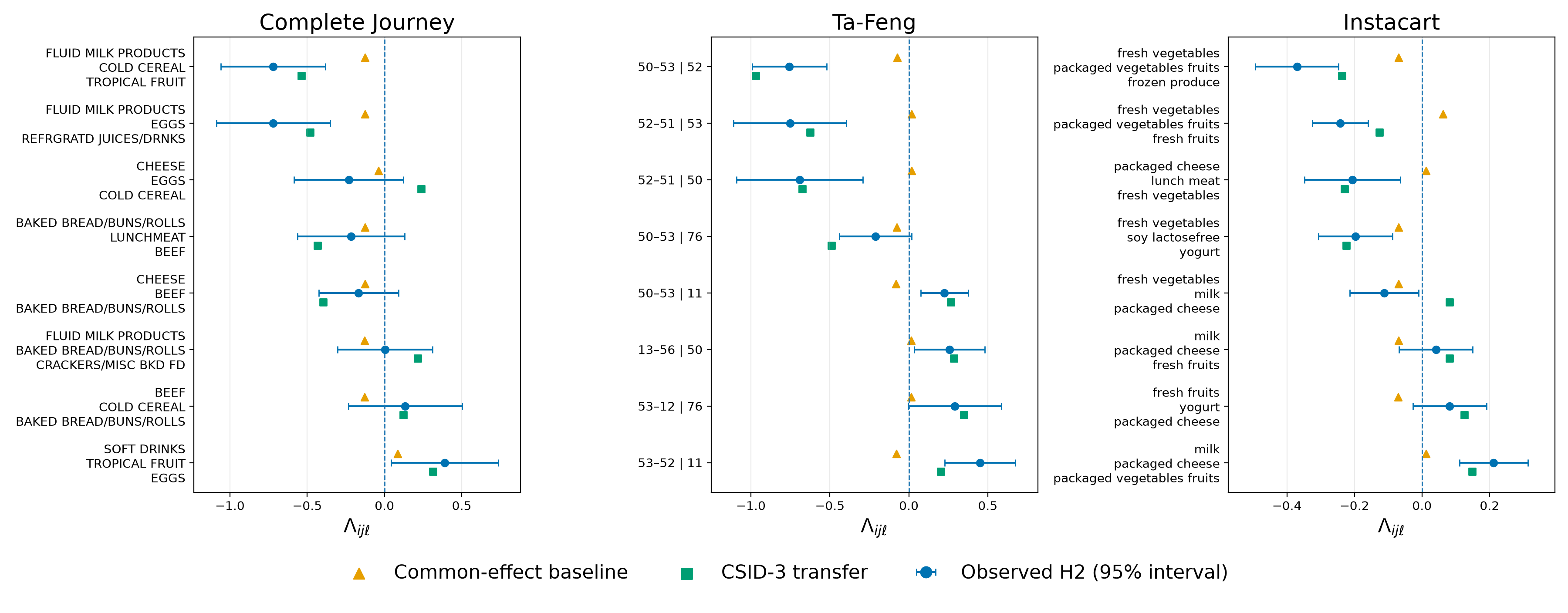
Figure 4 illustrates representative cases. For Milk–Cereal moderated by Tropical fruit in Complete Journey, the H2 contrast was $\widehat{\Lambda}^{\mathrm{H2}}=-0.721$, indicating a weaker conditional pair odds ratio when Tropical fruit was present. In Ta-Feng, the H2 contrast for pair 50–53 was negative with category 52 as moderator ($-0.757$) but positive with category 11 as moderator ($0.225$). In Instacart, Fresh vegetables–Packaged vegetables/fruits had a negative H2 contrast when moderated by Fresh fruits ($-0.242$).

Across the displayed examples, transferring CSID-3 generally reproduced the direction and approximate magnitude of the observed modulation better than the common-component baseline, although over- and under-estimation remained for small effects. Figure 4 is an interpretive visualization of the all-layer analysis in Tables 6 and 7, not an independent confirmatory test.

Applying eqs. 42 and 43 and refitting CSID-2 changed pairwise projections in both directions. Table 9 reports CSID-2, reweighted CSID-2, and their difference $\Delta\theta^{(3)}:=\widehat{\theta}^{\mathrm{reweighted}}-\widehat{\theta}^{\mathrm{CSID2}}$.

For Milk–Cold cereal and Ta-Feng pair 51–54, removing overlapping negative third-order effects strengthened the positive pairwise projection. For Fresh herbs–Cereal, the negative pairwise projection became stronger, indicating that positive third-order components had partly offset it before deprojection. Table 9 shows that the correction is therefore not a one-directional shrinkage reversal; it depends on the signs and locations of triples containing the pair.

To assess temporal stability, we applied H1 triple coefficients to H2 pair cells and compared the resulting correction with corrections using H2 coefficients and full-period coefficients. Table 10 shows that H1-based corrections correlated positively with corrections estimated independently in H2 and were strongly correlated with the full-period reference. The result indicates that the identity of the triples affecting each pair projection, and the direction of that effect, are not merely in-sample numerical adjustments.

The main analyses used 20 selected categories to obtain a compact and interpretable item space in each dataset. To examine whether the resulting interactions were artifacts of this truncation, we repeated the Instacart analysis while expanding the surrounding aisle universe from 20 to 40, 80, and all 134 aisles observed in the sampled users.

The focal top-20 aisles, the sampled users, the basket set, the H1–H2 split, and the focal pair and triple candidates were held fixed. Only the aisles contributing to the rest-cardinality context were expanded. All estimates were expressed in a common gauge defined by the information weights from the all-aisle analysis.

As shown in Tables 11 and 5, focal pair and third-order coefficients remained highly correlated with the all-aisle reference at every context size, with Pearson correlations above 0.95 even when only 20 context aisles were used, and increased further as the universe expanded. Third-order pairwise deprojection showed the same pattern.

These results indicate that the focal interaction structure obtained from the top-20 representation was not primarily induced by truncating the surrounding item universe. The gain in cross-period CCC was nevertheless larger in the 20-aisle representation ($\Delta\mathrm{CCC}=0.286$) than in the expanded contexts ($0.163$–$0.172$; Table 11). Because expanding the item universe changes the definition of rest cardinality and hence the stratified contrast itself, we interpret this difference as context dependence of the transfer metric rather than instability of the focal coefficients.

The main temporal-reproducibility, partial-transfer, and pair-correction conclusions were stable across the tested smoothing constants, ridge penalties, and minimum rest-cardinality choices; detailed results are reported in Appendix A.

In a candidate-restricted audit on 373,133 Instacart baskets, the implementation retained 156,735 supported triple candidates across 134 aisles and completed the measured stages in 49.9 seconds; full implementation settings, runtime, and storage results are reported in Appendix B.

References

- (1) R. Agrawal, T. Imieliński and A. Swami, Mining association rules between sets of items in large databases, in Proceedings of the 1993 ACM SIGMOD International Conference on Management of Data, pp. 207–216, 1993.
- (2) M.A. Valle, G.A. Ruz and S. Rica, Market basket analysis by solving the inverse Ising problem: Discovering pairwise interaction strengths among products, Physica A: Statistical Mechanics and its Applications 524 (2019) 36.
- (3) S. Brin, R. Motwani and C. Silverstein, Beyond market baskets: Generalizing association rules to correlations, in Proceedings of the 1997 ACM SIGMOD International Conference on Management of Data, pp. 265–276, 1997.
- (4) P.-N. Tan, V. Kumar and J. Srivastava, Selecting the right objective measure for association analysis, Information Systems 29 (2004) 293.
- (5) L. Geng and H.J. Hamilton, Interestingness measures for data mining: a survey, ACM Computing Surveys 38 (2006) no. 9.
- (6) X. Wu, D. Barbará and Y. Ye, Screening and interpreting multi-item associations based on log-linear modeling, in Proceedings of the Ninth ACM SIGKDD International Conference on Knowledge Discovery and Data Mining, pp. 276–285, 2003.
- (7) Y.M. Bishop, S.E. Fienberg and P.W. Holland, Discrete Multivariate Analysis: Theory and Practice, MIT Press, Cambridge, MA (1975).
- (8) G.F.V. Glonek and P. McCullagh, Multivariate logistic models, Journal of the Royal Statistical Society: Series B (Methodological) 57 (1995) 533.
- (9) W.P. Bergsma and T. Rudas, Marginal models for categorical data, The Annals of Statistics 30 (2002) 140.
- (10) J. Besag, Statistical analysis of non-lattice data, Journal of the Royal Statistical Society: Series D (The Statistician) 24 (1975) 179.
- (11) P. Ravikumar, M.J. Wainwright and J.D. Lafferty, High-dimensional Ising model selection using -regularized logistic regression, The Annals of Statistics 38 (2010) 1287.
- (12) E. Aurell and M. Ekeberg, Inverse Ising inference using all the data, Physical Review Letters 108 (2012) 090201.
- (13) H.C. Nguyen, R. Zecchina and J. Berg, Inverse statistical problems: from the inverse Ising problem to data science, Advances in Physics 66 (2017) 197 [1702.01522].
- (14) E. Schneidman, M.J. Berry, R. Segev and W. Bialek, Weak pairwise correlations imply strongly correlated network states in a neural population, Nature 440 (2006) 1007.
- (15) E. Ganmor, R. Segev and E. Schneidman, Sparse low-order interaction network underlies a highly correlated and learnable neural population code, Proceedings of the National Academy of Sciences 108 (2011) 9679.
- (16) F. Battiston, G. Cencetti, I. Iacopini, V. Latora, M. Lucas, A. Patania et al., Networks beyond pairwise interactions: structure and dynamics, Physics Reports 874 (2020) 1 [2006.01764].
- (17) F. Battiston, E. Amico, A. Barrat, G. Bianconi, G. Ferraz de Arruda, B. Franceschiello et al., The physics of higher-order interactions in complex systems, Nature Physics 17 (2021) 1093 [2110.06023].
- (18) C. Matias, A statistical perspective on higher-order interactions modeling, 2603.28273.
- (19) L. Betti, F. Musciotto, F. Battiston and R.N. Mantegna, Identifying maximal sets of significantly interacting nodes in higher-order networks, Physical Review E 114 (2026) 024313 [2209.12712].
- (20) H. Hruschka, Analyzing market basket data through sparse multivariate logit models, Journal of Marketing Analytics 14 (2026) 104.
- (21) P. Manchanda, A. Ansari and S. Gupta, The “shopping basket”: a model for multicategory purchase incidence decisions, Marketing Science 18 (1999) 95.
- (22) G.J. Russell and A. Petersen, Analysis of cross category dependence in market basket selection, Journal of Retailing 76 (2000) 367.
- (23) S.V. Beentjes and A. Khamseh, Higher-order interactions in statistical physics and machine learning: A model-independent solution to the inverse problem at equilibrium, Physical Review E 102 (2020) 053314.
- (24) A. Decelle, A.d.J. Navas Gómez and B. Seoane, Inferring higher-order couplings with neural networks, Physical Review Letters 135 (2025) 207301 [2501.06108].
- (25) C. de Mulatier and M. Marsili, Bayesian inference of minimally complex models with interactions of arbitrary order, 2008.00520.
- (26) A. De Clercq, M. Moody and C. de Mulatier, Modeling discrete data with high-order vector Potts models, 2606.03429.
- (27) R. Gupta, A.A. Diwan and S. Sarawagi, Efficient inference with cardinality-based clique potentials, in Proceedings of the 24th International Conference on Machine Learning, pp. 329–336, 2007, DOI.
- (28) D. Tarlow, K. Swersky, R.S. Zemel, R.P. Adams and B.J. Frey, Fast exact inference for recursive cardinality models, in Proceedings of the Twenty-Eighth Conference on Uncertainty in Artificial Intelligence, (Corvallis, OR), pp. 825–834, AUAI Press, 2012, https://www.auai.org/uai2012/papers/291.pdf.
- (29) K. Swersky, I. Sutskever, D. Tarlow, R.S. Zemel, R. Salakhutdinov and R.P. Adams, Cardinality restricted Boltzmann machines, in Advances in Neural Information Processing Systems 25, pp. 3302–3310, 2012.
- (30) A. Agresti, Categorical Data Analysis, Wiley, Hoboken, NJ, 3 ed. (2013).
- (31) A.W. van der Vaart, Asymptotic Statistics, Cambridge University Press, Cambridge (1998), 10.1017/CBO9780511802256.
- (32) R. Agrawal and R. Srikant, Fast algorithms for mining association rules, in Proceedings of the 20th International Conference on Very Large Data Bases, pp. 487–499, 1994.
- (33) J. Davis and M. Goadrich, The relationship between precision-recall and ROC curves, in Proceedings of the 23rd International Conference on Machine Learning, pp. 233–240, 2006, DOI.
- (34) B. Boehmke and S.M. Mortimer, completejourney: Retail Shopping Data, 2025.
- (35) C.-N. Hsu, H.-H. Chung and H.-S. Huang, Mining skewed and sparse transaction data for personalized shopping recommendation, Machine Learning 57 (2004) 35.
- (36) C. Das, “Ta-Feng grocery dataset.” https://www.kaggle.com/datasets/chiranjivdas09/ta-feng-grocery-dataset, 2020.
- (37) Instacart, “The Instacart online grocery shopping dataset 2017.” https://tech.instacart.com/3-million-instacart-orders-open-sourced-d40d29ead6f2, 2017.
- (38) P. Sparks, “Instacart market basket analysis.” https://www.kaggle.com/datasets/psparks/instacart-market-basket-analysis, 2017.
- (39) H. Höfling and R. Tibshirani, Estimation of sparse binary pairwise Markov networks using pseudo-likelihoods, Journal of Machine Learning Research 10 (2009) 883.
- (40) S. Mukherjee, J. Son and B.B. Bhattacharya, Estimation in tensor Ising models, Information and Inference: A Journal of the IMA 11 (2022) 1457 [2008.12882].
- (41) L.I.-K. Lin, A concordance correlation coefficient to evaluate reproducibility, Biometrics 45 (1989) 255.