FLARE: Flow Matching with Local Axis-Angle Representations for Stochastic Micromagnetic Evolution

Pengyu Li Email: These authors contributed equally to this work. Affiliation: State Key Laboratory of Quantum Functional Materials, Department of Physics, and Guangdong Basic Research Center of Excellence for Quantum Science, Southern University of Science and Technology, Shenzhen 518055, China Renjie Tong Email: These authors contributed equally to this work. Affiliation: State Key Laboratory of Quantum Functional Materials, Department of Physics, and Guangdong Basic Research Center of Excellence for Quantum Science, Southern University of Science and Technology, Shenzhen 518055, China Xuanlue Jiang Email: These authors contributed equally to this work. Affiliation: State Key Laboratory of Quantum Functional Materials, Department of Physics, and Guangdong Basic Research Center of Excellence for Quantum Science, Southern University of Science and Technology, Shenzhen 518055, China Jianmin Li Email: These authors contributed equally to this work. Affiliation: State Key Laboratory of Quantum Functional Materials, Department of Physics, and Guangdong Basic Research Center of Excellence for Quantum Science, Southern University of Science and Technology, Shenzhen 518055, China Yuanyuan Zhou Email: zhouyy3@sustech.edu.cn Affiliation: State Key Laboratory of Quantum Functional Materials, Department of Physics, and Guangdong Basic Research Center of Excellence for Quantum Science, Southern University of Science and Technology, Shenzhen 518055, China

Abstract

Long-horizon micromagnetic simulation remains expensive because conventional and learned solvers typically propagate Landau–Lifshitz–Gilbert (LLG) dynamics step by step. Existing learned approaches generally retain stepwise integration or model deterministic evolution, leaving full-field, direct-horizon stochastic prediction largely unexplored. We propose FLARE, a flow-matching framework that recasts stochastic finite-time magnetization prediction as conditional transport over anchor-relative local axis-angle rotations. This rotation-space formulation respects the intrinsic geometry of magnetization dynamics and preserves pointwise unit norm by construction. By explicitly conditioning on the physical prediction horizon, FLARE directly generates full-field stochastic endpoints across multiple target times without stepwise integration. Against the strongest single-checkpoint external baseline on each metric, FLARE achieves 29.9% lower angular energy distance ( $15.30^{\circ}$ ), and a 37.3% lower fair energy score (0.393). On a representative composed 5-ns two-segment protocol, FLARE achieves a $3{,}062\times$ best-batch speedup over the widely used GPU micromagnetic solver MuMax³ on a single GPU.

I Introduction

Magnetization dynamics can be viewed as a structured stochastic generative problem: given a current magnetization field, physical controls, and a target horizon, the goal is to predict the distribution of possible future states. Conventional micromagnetic solvers obtain these outcomes by integrating the Landau–Lifshitz–Gilbert (LLG) equation through many small time steps, making long-horizon and ensemble simulation expensive [22, 83, 28, 75, 10, 67].

Learned models can amortize this cost, but existing approaches largely focus on specialized magnetic tasks, sequential surrogate simulation, or deterministic prediction [39, 20, 84, 26, 12, 18, 17]. This leaves direct generation of full-field stochastic endpoints across physical horizons largely unexplored in micromagnetics.

We address this problem with FLARE , a conditional generative framework built around an anchor-relative rotational representation of magnetization change. Because each local magnetizaiton is contrained to the unit sphere, its finite-time change is naturally expressed relative to its current orientation. Rather than transporting absolute Cartesian future states, FLARE represents each transition as a field of local axis-angle rotations relative to the current magnetization. Conditional flow matching learns the distribution of these rotation fields [58], while Rodrigues decoding preserves pointwise unit norm by construction. Explicit physical-horizon conditioning enables a single model to generate stochastic endpoints across target times without stepwise LLG integration. Generated endpoints can further serve as anchors for subsequent control segments. Our contributions are: Anchor-relative rotation-field transport. We formulate stochastic finite-time magnetization transitions in local rotational coordinates relative to the anchor and instantiate this representation with axis-angle rotation fields. Matched controls isolate its advantage over Cartesian transport. Direct stochastic endpoint generation across horizons. We introduce horizon-conditioned stochastic endpoint generation as an alternative to sequential physical-time propagation, and demonstrate generalization to held-out horizons and self-generated anchors under changing controls. Multi-criteria evaluation framework. We develop a unified evaluation framework for stochastic dynamics that jointly measures sample-level field error, ensemble distribution fidelity, physical-observable distributions, and complete-output latency.

II Background and Related Work

Micromagnetic dynamics and numerical acceleration. Classical micromagnetics represents magnetic systems through a continuum magnetization field [9, 2]. The dynamics of the normalized magnetization are commonly governed by the Landau–Lifshitz–Gilbert (LLG) equation [51, 31]. At finite temperature, thermal fluctuations can be incorporated through stochastic field terms, leading to stochastic Landau–Lifshitz or LLG dynamics [65, 76, 52]. Established packages such as OOMMF, MuMax³, Fidimag, magnum.np, and MuMax+ numerically integrate these equations on CPU or GPU [22, 83, 7, 10, 67, 1]. Nevertheless, high-resolution, long-horizon, and ensemble simulations remain costly because resolving the dynamics requires propagating the full magnetization field through many successive physical time steps. Learned simulators and neural operators. Learned simulators reduce repeated simulation cost by approximating dynamical mappings from data, including graph- and mesh-based autoregressive models [78, 71, 86] and neural operators for PDE surrogate modeling [62, 56, 47, 85], as well as continuous-time, latent, and structure-preserving formulations of learned dynamics [88, 4, 11, 63, 13]; approximation-theoretic analyses further motivate neural surrogates for parametric PDEs [50]. In micromagnetics, learning has been applied to magnetostatic fields, inverse problems, energy minimization, reduced-order dynamics, and low-dimensional observables [48, 81, 79, 49, 25, 24, 80, 15, 21]. Hybrid approaches such as NeuralMAG and MagneX replace expensive field computations with neural surrogates while retaining sequential time integration [12, 69]; PDE-Refiner improves the stability of long-horizon neural PDE rollouts through iterative refinement, while likewise retaining sequential temporal propagation [59]. Existing learned approaches have largely focused on deterministic state prediction, reduced-order evolution, or accelerating components of sequential integration, rather than conditional distribution modeling of full-field finite-temperature dynamics.

Generative models and flow matching for stochastic dynamics. Generative surrogates extend learned simulation from point prediction to distributions over possible physical outcomes, with applications spanning fluid dynamics, PDE forecasting, molecular systems, and weather[45, 3, 77, 74, 46, 29, 91, 55, 38]. Recent examples include TurbDiff for turbulent flows, GenCast for ensemble weather prediction, MDGEN for molecular-dynamics trajectories, and MarS-FM for Markov-state molecular transitions [57, 72, 41, 42]. Flow Matching learns a continuous-time vector field that transports a simple source distribution to a target data distribution [58, 43], and has been applied to finite-horizon atomic transport composed into longer trajectories and to DFT Hamiltonian prediction [68, 44].

These studies establish generative modeling as a viable surrogate paradigm for stochastic physical dynamics. Micromagnetics introduces additional geometric structure: the state is a full spatial vector field at finite temperature, with each local magnetization constrained to lie on the unit sphere. Related geometric generative models accommodate manifold constraints through Riemannian score-based and diffusion processes [19, 37, 61], Riemannian flow matching [14, 89, 16], and Lie-group and structured-domain formulations [92, 8, 66, 6, 54]; generation of manifold-supported data has also been analyzed theoretically [60, 90]. FLARE instead models finite-time magnetization change in anchor-relative rotational coordinates, while retaining Euclidean flow matching and enforcing the spherical constraint exactly through rotation-based decoding. Unlike finite-horizon transport formulated in global Euclidean coordinates [68], FLARE defines these rotational coordinates locally with respect to the anchor magnetization at each spatial site.

Refer to caption — Figure 1: Overview of FLARE. a: During inference, ODE sampling transports an initial Gaussian rotation field $\Omega_{0}$ along the learned velocity field to the terminal rotation prediction $\widehat{\Omega}^{\star}=\Omega(1)$ . b: FLARE represents the transition from the anchor magnetization $\mathbf{m}_{s}$ to the target $\mathbf{m}_{t}$ as a local axis–angle rotation field $\Omega^{\star}$ and trains a conditional U-Net with self-attention using the CFM path $\Omega_{\tau}=(1-\tau)\Omega_{0}+\tau\Omega^{\star}$ . Spatial conditions $F$ are concatenated with $\Omega_{\tau}$ and $\mathbf{m}_{s}$ , while the flow time $\tau$ , physical horizon $\Delta t$ , and global conditions $c_{g}$ are injected through AdaGroupNorm. c: The sampled terminal rotation field is mapped back to magnetization space through Rodrigues rotation. For multi-segment dynamics, each generated endpoint is recursively used as the anchor of the next FLARE call under the corresponding segment conditions.

III FLARE

III.1 Problem setup

We consider a three-component unit magnetization field $\mathbf{m}:\Omega\times[0,S]\to\mathbb{S}^{2}$ on a two-dimensional spatial domain $\Omega\subset\mathbb{R}^{2}$ . Its evolution is governed by the stochastic LLG equation [51, 31]

	$\displaystyle\frac{\partial\mathbf{m}}{\partial t}$	$\displaystyle=-\gamma\,\mathbf{m}\times H_{\mathrm{eff}}(\mathbf{m};\eta,\xi_{t})$		(1)
		$\displaystyle+\alpha\,\mathbf{m}\times\frac{\partial\mathbf{m}}{\partial t}+T(\mathbf{m};u(t),\eta).$		(1)

where $\|\mathbf{m}(\mathbf{r},t)\|_{2}=1$ , $\mathbf{r}$ denotes spatial position and $t$ denotes the physical time. Here, $\gamma$ is the gyromagnetic ratio, $\alpha$ is the Gilbert damping coefficient, $\xi_{t}$ denotes finite-temperature stochastic forcing in $H_{\mathrm{eff}}$ , $T$ is spin torque and $u(t)$ denotes controls such as external fields or currents, and $\eta$ collects static system parameters such as material properties and geometry. Given an anchor magnetization field ( $\mathbf{m}(t)$ ), a physical condition ( $c$ ), and a target horizon ( $\Delta\!t$ ), our goal is to model the conditional distribution:

p\!\left(\mathbf{m}{(t+\Delta\!t)}\mid\mathbf{m}_{t},c,\Delta\!t\right),

(2)

where $c=(c_{g},F)$ denotes the physical condition, with $c_{g}$ containing global or segment-level controls and $F$ encoding spatially resolved conditions such as geometry and local driving. A single query therefore produces a future state at the requested physical horizon. We use trajectory exclusively for a time-resolved simulator evolution, segment endpoint for a state at a control boundary, and generated state sequence for recursively composed predictions.

Realistic simulation protocols may contain multiple stages with different physical controls. We represent such a protocol as $K$ conditionally defined segments with conditions $(c^{k})_{k=1}^{K}$ , where each $c^{k}$ specifies the physical environment and duration of the $k$ -th segment. Multi-stage generation is then defined recursively as:

\begin{gathered}\hat{\mathbf{m}}^{(0)}=\mathbf{m}_{0},\\ \hat{\mathbf{m}}^{(k)}\sim p_{\theta}\left(\mathbf{m}\mid\hat{\mathbf{m}}^{(k-1)},c^{(k)}\right),\\ k=1,\ldots,K.\end{gathered}

(3)

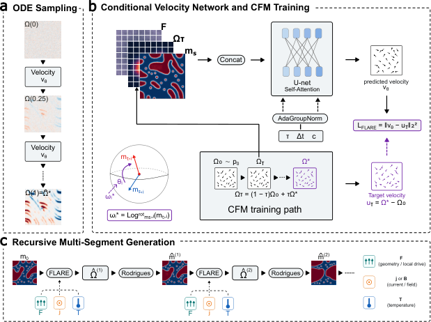
Each generated endpoint serves as the anchor for the subsequent segment, and the resulting sequence $(\hat{\mathbf{m}}^{(k)})_{k=1}^{K}$ forms a generated state sequence across the prescribed multi-stage protocol.

III.2 Model formulation

Local Axis-Angle Transition Representation.

The overall architecture and generation pipeline of FLARE are illustrated in Figure 1. Each magnetic moment satisfies $\mathbf{m}_{s,i},\mathbf{m}_{t,i}\in S^{2}$ . Rather than representing finite-time magnetization change as an unconstrained Cartesian displacement, we represent the transition from the anchor $\mathbf{m}_{s,i}$ to the target $\mathbf{m}_{t,i}$ by their principal axis-angle rotation [53, 23]:

\begin{gathered}\theta_{i}=\operatorname{atan2}\left(\left\|\mathbf{m}_{s,i}\times\mathbf{m}_{t,i}\right\|_{2},\mathbf{m}_{s,i}^{\mathsf{T}}\mathbf{m}_{t,i}\right),\\ \bm{\omega}_{i}^{\star}=\theta_{i}\frac{\mathbf{m}_{s,i}\times\mathbf{m}_{t,i}}{\left\|\mathbf{m}_{s,i}\times\mathbf{m}_{t,i}\right\|_{2}}.\end{gathered}

(4)

We denote this anchor-relative rotation encoding by $\bm{\omega}_{i}^{\star}=\operatorname{Log}^{\mathrm{rot}}_{\mathbf{m}_{s,i}}(\mathbf{m}_{t,i})$ . For the ideal encoding, $\bm{\omega}_{i}^{\star}\perp\mathbf{m}_{s,i}$ and $\|\bm{\omega}_{i}^{\star}\|_{2}=\theta_{i}\in[0,\pi]$ , so its direction specifies the local rotation axis and its magnitude the principal rotation angle. Given $\theta=\|\bm{\omega}\|_{2}$ and $\mathbf{a}=\bm{\omega}/\theta$ , the corresponding rotation is reconstructed through Rodrigues’ formula [33, 30]

\begin{gathered}\mathcal{R}(\bm{\omega})=\mathbf{I}+\sin\theta[\mathbf{a}]_{\times}+(1-\cos\theta)[\mathbf{a}]_{\times}^{2},\\ \mathbf{m}_{t,i}=\mathcal{R}(\bm{\omega}_{i}^{\star})\mathbf{m}_{s,i}.\end{gathered}

(5)

Because $\mathcal{R}(\bm{\omega})\in SO(3)$ , the reconstruction preserves the pointwise unit norm of the magnetization by construction. For nearly identical moments, we use the first-order limit $\bm{\omega}_{i}^{\star}\approx\mathbf{m}_{s,i}\times\mathbf{m}_{t,i}$ . Near antipodal configurations, we adopt a deterministic tangent-axis $\pi$ -rotation approximation. Implementation details and statistics for these corner cases are provided in Appendix A.1. The resulting rotation field $\Omega^{\star}=\{\bm{\omega}_{i}^{\star}\}_{i=1}^{N}$ serves as the representation on which the conditional flow model is defined.

Conditional Flow Matching in Rotation Space

Given the endpoint rotation field $\bm{\Omega}^{\star}$ , we sample a Gaussian source $\bm{\Omega}_{0}\sim p_{0}$ and a flow time $\tau\sim\mathcal{U}(0,1)$ and construct the straight conditional path [58, 82]

\bm{\Omega}_{\tau}=(1-\tau)\bm{\Omega}_{0}+\tau\bm{\Omega}^{\star},\qquad\mathbf{u}_{\tau}=\frac{\partial\bm{\Omega}_{\tau}}{\partial\tau}=\bm{\Omega}^{\star}-\bm{\Omega}_{0}.

(6)

Here, $\tau\in[0,1]$ denotes the generative flow time and is distinct from the physical prediction horizon $\Delta t$ . We learn a conditional vector field $\mathbf{v}_{\theta}\left(\bm{\Omega}_{\tau},\tau\mid\mathbf{m}_{s},\Delta t,c_{g},\mathbf{F}\right)$ to approximate the target velocity $\mathbf{u}_{\tau}$ . The model is trained with a conditional flow-matching objective

\mathcal{L}_{\mathrm{FLARE}}=\mathbb{E}\left[\left|\mathbf{v}_{\theta}\left(\bm{\Omega}_{\tau},\tau\mid\mathbf{m}_{s},\Delta t,c_{g},\mathbf{F}\right)-\mathbf{u}_{\tau}\right|_{2}^{2}\right],

(7)

where the expectation is taken over training transitions, Gaussian source samples, and flow times. Uniform weighting is used across sampled flow times, prediction horizons, and driving categories.

In inference, we integrate the learned vector field in rotation space,

\frac{d\bm{\Omega}}{d\tau}=\mathbf{v}_{\theta}\left(\bm{\Omega},\tau\mid\mathbf{m}_{s},\Delta t,c_{g},\mathbf{F}\right),\qquad\bm{\Omega}(0)=\bm{\Omega}_{0},

(8)

to obtain the terminal rotation field $\widehat{\bm{\Omega}}^{\star}=\bm{\Omega}(1)$ . The sampled rotation need not be the minimal one, since $\|\widehat{\bm{\omega}}_{i}^{\star}\|_{2}$ may exceed $\pi$ , but Rodrigues decoding still returns a unit vector at every cell; see Eq. 5.

Conditional Vector-Field Network

We parameterize $\mathbf{v}_{\theta}$ with a U-Net at native spatial resolution. Its spatial input concatenates the anchor magnetization $\mathbf{m}_{s}$ , rotation state $\Omega_{\tau}$ , and full-resolution condition features $F$ , yielding 19 input channels. The feature maps $\mathbf{F}$ encode spatially resolved information such as geometry and position-dependent driving fields.

Global conditioning is handled separately. The flow time $\tau$ , target horizon $\Delta t$ , and segment-level physical controls $c_{g}$ are embedded into a 512-dimensional conditioning vector, which modulates the U-Net features at each resolution through AdaGroupNorm. An eight-head self-attention block at the bottleneck captures long-range spatial dependencies. The network outputs a three-channel velocity field $\mathbf{v}_{\theta}\left(\bm{\Omega}_{\tau},\tau\mid\mathbf{m}_{s},\Delta t,c_{g},\mathbf{F}\right),$ which parametrizes the generative ODE in Eq. 8.

Training-Pair Construction

We partition each trajectory at changes in the driving protocol and sample training pairs within individual constant-control segments. After uniformly sampling a valid trajectory and target type, we sample a valid anchor $s$ and candidate horizon $h$ ; the target is the saved frame nearest $s+h$ that remains within the same segment. The actual timestamp difference defines the physical horizon, $\Delta t=t_{\mathrm{target}}-t_{\mathrm{anchor}}$ , yielding a training tuple $(\mathbf{m}_{s},\mathbf{m}_{t},\Delta t,c_{g},F)$ , where $c_{g}$ denotes the corresponding segment conditions. For validation, we use the earliest valid anchor in each admissible range, yielding a deterministic protocol aligned with rollout from the segment start.

III.3 Distributional Evaluation Metric.

Magnetization dynamics are stochastic, so agreement with a single MuMax³ realization is insufficient to assess whether a generative model captures the distribution of physically plausible outcomes. We therefore define a distributional metric that compares sets of magnetization fields while accounting for small spatial displacements of otherwise similar magnetic textures.

Local translation-matching distance

Direct cell-wise distance can strongly penalize small translations of domain walls, vortices, or other localized structures. To obtain a more structure-aware comparison, we adopt a local translation-matching procedure inspired by displacement search in image registration and block matching [40, 93, 5]. As illustrated in Figure 3, the magnetization field is partitioned into local patches, and each patch is independently matched over a bounded translation window. For normalized magnetization fields $\mathbf{m}_{a}$ and $\mathbf{m}_{b}$ , we define

\begin{gathered}C_{p}^{a\to b}=\max_{\Delta r\in\mathcal{W}}\frac{1}{|\Omega_{p}|}\sum_{r\in\Omega_{p}}m_{a}(r)\!\cdot\!m_{b}(r+\Delta r),\\ D(a,b)=\frac{1}{2P_{\rm patch}}\sum_{p=1}^{P_{\rm patch}}\left(2-C_{p}^{a\to b}-C_{p}^{b\to a}\right).\end{gathered}

(9)

where $\Omega_{p}$ denotes the spatial support of patch $p$ and $\mathcal{W}$ is the allowed translation window. Locations shifted outside the magnetic geometry contribute zero. The symmetric distance $D(a,b)$ therefore measures disagreement in the local magnetic structure while remaining tolerant to small spatial translations.

Distribution Score.

For a fixed physical condition, let $X=\{x_{i}\}_{i=1}^{M}$ and $Y=\{y_{j}\}_{j=1}^{N}$ denote the reference MuMax³ outcomes and the model outcomes, respectively. We convert pairwise distance $D$ into a Gaussian similarity. For each MuMax³ outcome $x_{i}$ , we then estimate two local densities: one induced by the model-generated samples and a leave-one-out reference density estimated from the remaining MuMax³ repeats. The kernel bandwidth is determined solely from nearest-neighbor distances among the MuMax³ samples, so that the metric does not depend on the model outputs. The complete kernel and density definitions are provided in Appendix B.

Using these densities, the per-condition agreement score and the final Distribution Score are

	$\displaystyle S_{c}$	$\displaystyle=\exp\left[-\frac{1}{M}\sum_{i=1}^{M}\left\|\log\frac{q_{\mathrm{model}}(x_{i})+\epsilon}{q_{\mathrm{MuMax}}^{-i}(x_{i})+\epsilon}\right\|\right],$		(10)
	$\displaystyle S_{\mathrm{dist}}$	$\displaystyle=\exp\left[\frac{1}{N_{\mathrm{cond}}}\sum_{c=1}^{N_{\mathrm{cond}}}\log S_{c}\right],$		(10)

where $\epsilon=10^{-12}$ . The resulting distribution score lies in $(0,1]$ , with values closer to one indicating better agreement between the generated and MuMax³ endpoint distributions.

IV Experiments

IV.1 Experimental Setup

Dataset and splits.

We evaluate FLARE on a finite-temperature micromagnetic dataset generated with MuMax³, comprising 7,770 completed driven and post-drive-relaxation trajectories from 1,000 base conditions. Each state is a three-component magnetization field on a $256\times 256\times 1$ finite-difference grid corresponding to a $512\times 512\times 1$ $\mathrm{nm}^{3}$ magnetic film with open boundaries. The configured 1–6 ns interval refers to absolute simulation times rather than one-shot prediction horizons. The material parameters are fixed across the corpus and include interfacial Dzyaloshinskii–Moriya interaction, while temperature, out-of-plane field, current amplitude, initial texture, and the spatial current-mask family are varied. Detailed material parameters, control ranges, temperature levels, and the distribution over the five mask families are given in Appendix A. To avoid leakage between trajectories generated under the same physical setting, we partition by base condition, resulting in 6,227 training, 786 validation, and 757 test trajectories.

Comparators and execution protocol.

We compare FLARE with author-released CNO [73], Poseidon [36], DPOT [35], MPP [64], PDEArena [34], LE-PDE [87], and NeuralMAG [12]. These external comparators are deterministic per checkpoint, except for NeuralMAG-x5, which retains the thermal field; the two matched internal controls change only the transport coordinates or the learning objective. All learned models are adapted to the same x5 training split for 50,000 optimization updates and use the final checkpoint. Quality follows the exact-control complete path: each method predicts the driven segment from the saved pre-drive state, passes its own boundary prediction into the exact 3.5-ns relaxation, and is scored only at the final endpoint. No MuMax³ state is injected at the handoff. Because complete-path durations vary, timing uses a separate standardized fixed two-segment 5-ns workload: a 2-ns driven segment followed by a 3-ns zero-current relaxation, with the first segment’s model prediction handed to the second. Each method keeps its native temporal interface. We report both batch-one latency and the minimum per-output latency over a power-of-two batch sweep; MuMax³ is timed in its standard single-process execution mode, where $B{=}1$ is its fastest per-output setting.

Metrics and uncertainty.

Distribution fidelity is evaluated over 33 held-out complete-path conditions, each with five repeat trajectories. We use complementary diagnostics comprising the Distribution Score defined in Sec. III.3, angular energy distance, and the proper fair energy score [32, 27]. Distribution Score and angular energy distance compare the five final model endpoints with the five corresponding MuMax³ endpoints as outcome sets, while paired angle matches repeat $i$ and is retained as a realization-level diagnostic. Paired angle is minimized by a deterministic central estimate of the conditional distribution and equals the MuMax³ repeat-to-repeat level for a correct sample. The proper fair energy score uses 165 exact drive-start anchors (33 bases $\times$ five repeats), with five forecasts per anchor for stochastic methods and a one-point forecast distribution for deterministic single checkpoints. Because the primary x5 set contains only one MuMax³ continuation per exact drive-start anchor, independent final-endpoint reference levels are estimated from the separate x30 audit (Appendix Table 7), which provides an absolute scale. We report 95% base-condition-clustered bootstrap intervals, retaining all five complete paths within each resampled base group. Angular error is the mean full-vector angular deviation, in degrees, over valid magnetic cells. The physical forecast spans range from 3.75 to 4.42 ns (mean 4.10 ns), reflecting the realized driven-segment durations followed by the exact 3.5-ns relaxation. Further resampling details are given in Appendix A.

IV.2 Main Results

Table 1: Single-checkpoint exact-control complete-path future-state quality; standardized fixed two-segment 5-ns timing. Every learned row uses 50,000 x5 updates; NeuralMAG-x5 retains the thermal field during both training and inference. Brackets are 95% base-group cluster-bootstrap intervals. External rows are single checkpoints; Table 15 reports five-seed ensembles of the same baselines, where FLARE’s fair-energy margin is 21.8%. The top row is a simulator-only reference (17-base

\times

30 audit; Appendix Table 7): a descriptive scale, not a ranked entry.

Method	$B{=}1$ latency (ms)	Distribution Score $\uparrow$	Paired angle (^∘) $\downarrow$	Angular energy dist. (^∘) $\downarrow$	Fair energy score $\downarrow$	$B{=}1$ speedup $\uparrow$	Best-batch speedup $\uparrow$
Reference
MuMax³ 5 vs 5	–	0.862 [0.801, 0.915]	30.25 [23.89, 36.66]	12.20 [9.62, 14.86]	–	–	–
FLARE ODE-10	995.2	0.762 [0.660, 0.844]	36.72 [31.93, 41.38]	15.30 [13.32, 17.26]	0.393 [0.356, 0.430]	$448.3\times$	$3{,}062.4\times$
Poseidon-T	61.91	0.341 [0.077, 0.749]	35.60 [30.60, 41.11]	25.05 [17.86, 34.56]	0.751 [0.672, 0.830]	$7{,}206.3\times$	$686{,}423.6\times$
CNO-FM	72.89	0.695 [0.577, 0.787]	34.43 [30.41, 38.33]	21.82 [17.94, 26.23]	0.745 [0.682, 0.807]	$6{,}120.7\times$	$133{,}012.0\times$
DPOT-Ti	91.13	0.707 [0.599, 0.803]	39.81 [34.46, 45.59]	27.02 [19.98, 36.58]	0.814 [0.735, 0.893]	$4{,}895.3\times$	$48{,}327.7\times$
MPP-AViT-Ti	613.4	0.290 [0.059, 0.764]	49.41 [43.24, 56.21]	42.10 [32.57, 52.93]	0.930 [0.849, 1.015]	$727.3\times$	$3{,}730.7\times$
PDEArena U-Net	40.17	0.597 [0.394, 0.779]	37.26 [32.48, 42.16]	24.03 [19.43, 28.99]	0.774 [0.697, 0.850]	$11{,}106.1\times$	$45{,}720.7\times$
LE-PDE	7.642	0.0018 [0.0001, 0.0293]	76.18 [70.31, 81.78]	77.96 [65.49, 91.87]	1.269 [1.207, 1.328]	$58{,}379.6\times$	$\mathbf{1{,}749{,}670.6\times}$
NeuralMAG-x5	335,786	0.316 [0.068, 0.731]	53.54 [47.41, 59.54]	36.76 [29.05, 45.58]	0.627 [0.562, 0.690]	$1.33\times$	$14.2\times$
Matched internal controls
FLARE (Cartesian)	–	0.711 [0.563, 0.821]	39.88 [35.54, 44.21]	17.91 [15.52, 20.48]	0.420 [0.383, 0.456]	–	–
Direct U-Net	–	0.477 [0.190, 0.783]	38.53 [34.44, 42.76]	21.41 [18.17, 24.91]	0.808 [0.745, 0.867]	–	–

Quality follows the protocol above. Cartesian CFM and Direct U-Net are internal controls: one changes coordinates; the other directly regresses $\Omega_{\star}$ . All three use seed 78. Because quality-path durations vary, timing uses a fixed two-segment representative 5-ns workload (2 ns drive plus 3 ns relaxation, with one predicted-state handoff): $B=1$ is single-query latency, best batch is the fastest supported power of two, and speedups use the 446.125-s MuMax³ reference. Neither control has timing; Table 2(a) gives the three-seed summary; Appendix Table 15 reports five-seed ensembles.

In Table 1, FLARE leads all seven author-released baselines on the three distributional metrics. Its Distribution Score is 0.762 versus 0.707 for DPOT-Ti (+7.9%); its angular energy distance is 15.30^∘ versus 21.82^∘ for CNO-FM (29.9% lower); and its fair energy score is 0.393 versus 0.627 for NeuralMAG-x5 (37.3% lower). CNO-FM obtains a lower repeat-paired angle, 34.43^∘ versus 36.72^∘; this metric scores one indexed stochastic realization rather than the unordered outcome distribution. Matched Cartesian CFM and Direct U-Net test the rotation coordinates and flow-matching objective, respectively. FLARE also leads five-model ensembles in distributional fidelity (Table 15). FLARE achieves a $3{,}062\times$ best-batch speedup (448× at B=1) over MuMax³ on the 5-ns workload (Table 1). On the driven segment (the only one with an exact-anchor oracle), FLARE’s fair energy score is 0.322 [0.290, 0.353] versus 0.283 [0.230, 0.335] for the MuMax³ reference. Single-segment diagnostics are reported in Appendices C.2–C.3. Multi-segment Composition. FLARE composes conditional endpoint distribution across changing controls by using each generated endpoint as the anchor for next segment, without intermediate LLG states. We evaluate both ground-truth-boundary and autoregressive handoffs over 736 rollouts from 97 held-out conditions. Predicted-state exposure improves autoregressive robustness over Stage 1 but does not outperform an equal-budget ground-truth-only continuation; we therefore treat it as an ablation rather than a separation contribution. Full results are provided in Appendix F and Table 17.

IV.3 Out-of-Distribution Generalization

We evaluate OOD generalization beyond the training distribution along two complementary axes: unseen spatial current-mask family and unseen temperature.

Unseen current-mask family.

We train a dedicated Stage 1 FLARE model after excluding all ring-current-mask conditions from training and validation. On the held-out ring-mask family, single-segment and autoregressive angular errors increase by $0.91^{\circ}$ (3.12%) and $0.95^{\circ}$ (3.04%), respectively, relative to the in-distribution reference. This indicates stable transfer to an unseen current-mask family. Full results are reported in Appendix G.

Unseen temperature.

Using the frozen Stage 1 checkpoint trained only at 30, 150, and 300 K, we evaluate new zero-shot test sets at 90 and 225 K. Relative to paired interpolation references from the adjacent training temperatures, single-segment and autoregressive angular errors change by $+1.27\%$ and $-4.15\%$ at 90 K, and by $+1.64\%$ and $+2.37\%$ at 225 K. No evaluated metric shows statistically resolved adverse degradation at either temperature, showing robust interpolation to unseen in-range physical conditions. Full metrics, confidence intervals, and the 400 K extrapolation stress test are reported in Appendix H.

IV.4 Ablation Studies

We isolate four design choices with matched controls: learned endpoint dynamics, anchor-relative rotational coordinates, physical-horizon conditioning, and the flow-matching objective (Table 2; Appendix E). Persistence is a no-dynamics sanity check; learned controls share the architecture and training budget unless stated otherwise. The compute-matched rollout-state control is reported separately in Appendix F.

Table 2: Stage 1 ablations. (a,b) Exact-control complete paths; (c) single-segment time interpolation. Panel (a) reports mean

\pm

sample SD over seeds 78–80; (b,c) report seed-78 point estimates.

(a) Representation and objective controls: three training seeds
Variant	Distribution Score $\uparrow$	Angular energy dist. (^∘) $\downarrow$	Paired angle (^∘) $\downarrow$	Fair energy score $\downarrow$
FLARE	$\bm{0.7592\pm 0.0056}$	$\bm{15.31\pm 0.24}$	$\bm{36.70\pm 0.23}$	$\bm{0.3944\pm 0.0028}$
FLARE(Fixed 2D tangent)	$0.7562\pm 0.0221$	$16.70\pm 2.09$	$37.94\pm 1.41$	$0.3991\pm 0.0155$
Cartesian CFM	$0.7176\pm 0.0073$	$17.98\pm 0.12$	$39.96\pm 0.29$	$0.4210\pm 0.0033$
Riemannian FM	$0.7341\pm 0.0071$	$18.00\pm 0.19$	$39.01\pm 0.10$	$0.4330\pm 0.0029$
Direct U-Net	$0.4741\pm 0.0040$	$21.26\pm 0.13$	$38.60\pm 0.07$	$0.8087\pm 0.0013$

(b) Component ablations
Design	Metrics	FLARE	Control	Gain
Flow transport	Angle (^∘) / MSE	36.74 / 0.6127	67.03 / 1.4045	+30.29 / +0.7918
Rotation coords.	Angle (^∘) / $\|\Delta Q\|$	36.74 / 0.7715	39.88 / 0.8786	+3.15 / +0.1071
Target time	Angle (^∘) / $\|\Delta\mathcal{E}\|$	36.74 / 0.00977	47.16 / 0.01145	+10.42 / +0.00167
(c) Time interpolation
1.5 / 2.5 ns	Angle (^∘)	30.88 / 32.67	39.79 / 40.97	+8.91 / +8.31

(a,b): 33 bases $\times$ five endpoints, predicted drive-to-relaxation handoff, 3.5-ns relaxation; fair energy uses 165 anchors with five stochastic draws or one deterministic forecast. (b) Controls: persistence, Cartesian CFM, no-time. (c): 256 cases per horizon, true segment starts, no-time control.

As shown in Table 2(b), the persistence comparison confirms that FLARE learns conditional dynamics beyond copying the anchor. Both the 3D axis–angle and fixed 2D tangent outperform absolute-spin Cartesian CFM and Riemannian FM across all four metrics (Table 2(a)), associating the gain with rotational coordinates rather than dimensionality. We use the 3D form to avoid per-spin tangent frames and reduce seed variability. Target-horizon conditioning improves both complete-path predictions and interpolation at the held-out 1.5- and 2.5-ns horizons.

V Discussion and Limitations

FLARE provides evidence that anchor-relative rotational coordinates are effective for modeling finite-temperature micromagnetic dynamics as conditional future-state distributions. At a matched five-sample budget, FLARE closely reproduces several physical-observable distributions, including topological charge and mean out-of-plane magnetization. FLARE also supports prediction-only composition across changing control segments, recursively using generated endpoints as subsequent anchors. Three-seed complete-path results favor the core model over Cartesian CFM, Riemannian FM, and Direct U-Net, while the ablations confirm the importance of explicit target-horizon conditioning. FLARE’s advantage is distributional fidelity for stochastic future-state prediction: CNO-FM achieves a lower paired angular error, and several deterministic surrogates are substantially faster at inference.

Several limitations remain. First, sequential composition introduces additional error under predicted-state handoffs, and mixed rollout-state exposure does not outperform the equal-budget GT-only continuation, leaving extended multi-segment composition sensitive to accumulated handoff error. Second, the present dataset covers a fixed material system and a limited range of temperatures, fields, currents, initial textures, and control geometries, so our results speak to that regime; extending it across materials and dynamical regimes requires new training data. Third, our experiments are restricted to two-dimensional thin-film micromagnetics and finite prediction horizons. Extension to three-dimensional systems, broader material and control distributions, and larger-scale training data is a natural direction for future work.

References

[1] C. Abert, F. Bruckner, A. Voronov, M. Lang, S. A. Pathak, S. Holt, R. Kraft, R. Allayarov, P. Flauger, S. Koraltan, T. Schrefl, A. Chumak, H. Fangohr, and D. Suess (2025) NeuralMag: an open-source nodal finite-difference code for inverse micromagnetics. npj Computational Materials 11, pp. 193. External Links: Document Cited by: Appendix K, §II.
[2] C. Abert (2019) Micromagnetics and spintronics: models and numerical methods. The European Physical Journal B 92, pp. 120. External Links: Document Cited by: §II.
[3] M. Andrae, T. Landelius, J. Oskarsson, and F. Lindsten (2025) Continuous Ensemble Weather Forecasting with Diffusion Models. In International Conference on Learning Representations, External Links: Link Cited by: §II.
[4] O. Azencot, N. B. Erichson, V. Lin, and M. W. Mahoney (2020) Forecasting Sequential Data Using Consistent Koopman Autoencoders. In International Conference on Machine Learning, External Links: Link Cited by: §II.
[5] C. Barnes, E. Shechtman, A. Finkelstein, and D. B. Goldman (2009) PatchMatch: a randomized correspondence algorithm for structural image editing. ACM Transactions on Graphics 28 (3), pp. 24:1–24:11. External Links: Document Cited by: §III.3.
[6] M. Bertolini, T. A. Le, and D. Clevert (2025) Diffusion generative modeling on Lie group representations. In Advances in Neural Information Processing Systems, Vol. 38. External Links: Document Cited by: §II.
[7] M. Bisotti, D. Cortés-Ortuño, R. A. Pepper, W. Wang, M. Beg, T. Kluyver, and H. Fangohr (2018) Fidimag–a finite difference atomistic and micromagnetic simulation package. Journal of Open Research Software 6 (1), pp. 22. External Links: Document, Link Cited by: Appendix K, §II.
[8] A. J. Bose, T. Akhound-Sadegh, G. Huguet, K. Fatras, J. Rector-Brooks, C. Liu, A. C. Nica, M. Korablyov, M. M. Bronstein, and A. Tong (2024) SE(3)-stochastic flow matching for protein backbone generation. In International Conference on Learning Representations, External Links: Link Cited by: §II.
[9] W. F. Jr. Brown (1963) Micromagnetics. Interscience Publishers, New York. Cited by: §II.
[10] F. Bruckner, S. Koraltan, C. Abert, and D. Suess (2023) Magnum. np: a pytorch based gpu enhanced finite difference micromagnetic simulation framework for high level development and inverse design. Scientific Reports 13 (1), pp. 12054. External Links: Document, Link Cited by: Appendix K, §I, §II.
[11] J. Bruna, B. Peherstorfer, and E. Vanden-Eijnden (2024) Neural Galerkin Schemes with Active Learning for High-Dimensional Evolution Equations. Journal of Computational Physics 496, pp. 112588. External Links: Link Cited by: §II.
[12] Y. Cai, J. Li, and D. Wang (2024) Fast and generalizable micromagnetic simulation with deep neural nets. Nature Machine Intelligence 6 (11), pp. 1330–1343. External Links: Document, Link Cited by: Appendix K, §I, §II, §IV.1.
[13] F. Carnazza, F. Carollo, S. Andergassen, G. Martius, M. Klopotek, and I. Lesanovsky (2024) Machine Learning Stochastic Differential Equations for the Evolution of Order Parameters of Classical Many-Body Systems in and out of Equilibrium. Machine Learning: Science and Technology 5, pp. 045002. External Links: Link, Document Cited by: §II.
[14] R. T. Q. Chen and Y. Lipman (2024) Flow matching on general geometries. In International Conference on Learning Representations, External Links: Link Cited by: Appendix E, §II.
[15] X. Chen, F. Abreu Araujo, M. Riou, J. Torrejon, D. Ravelosona, W. Kang, W. Zhao, J. Grollier, and D. Querlioz (2022) Forecasting the outcome of spintronic experiments with neural ordinary differential equations. Nature Communications 13, pp. 1016. External Links: Document, Link Cited by: Appendix K, §II.
[16] C. Cheng, Y. Wang, Y. Chen, X. Zhou, N. Zheng, and G. Liu (2025) Riemannian consistency model. In Advances in Neural Information Processing Systems, Vol. 38. External Links: Document Cited by: §II.
[17] G. Chern, Y. Fan, S. Zhang, and P. Zhang (2026) Machine-learning force-field models for dynamical simulations of metallic magnets. AIP Advances 16 (2), pp. 025031. External Links: Document Cited by: Appendix K, §I.
[18] G. Chern, Y. Fan, S. Zhang, and P. Zhang (2026) Machine-learning modeling of magnetization dynamics in quasi-equilibrium and driven metallic spin systems. Journal of Magnetism and Magnetic Materials 642, pp. 173898. External Links: Document Cited by: §I.
[19] V. De Bortoli, E. Mathieu, M. Hutchinson, J. Thornton, Y. W. Teh, and A. Doucet (2022) Riemannian score-based generative modelling. In Advances in Neural Information Processing Systems, Vol. 35, pp. 2406–2422. External Links: Document Cited by: §II.
[20] A. Y. Deviatov, I. A. Iakovlev, and V. V. Mazurenko (2019) Recurrent network classifier for ultrafast skyrmion dynamics. Physical Review Applied 12, pp. 054026. External Links: Document, Link Cited by: Appendix K, §I.
[21] S. Dolui and M. Salman (2026) A neural network framework for modeling the dynamics of the landau–lifshitz–gilbert equation. Engineering Applications of Artificial Intelligence 181 (4), pp. 115562. Note: In press; issue date 1 October 2026 External Links: Document, Link Cited by: Appendix K, §II.
[22] M. J. Donahue and D. G. Porter (1999) OOMMF user’s guide, version 1.0. NIST Interagency Report Technical Report NISTIR 6376, National Institute of Standards and Technology, Gaithersburg, MD. External Links: Document, Link Cited by: Appendix K, §I, §II.
[23] M. d’Aquino, C. Serpico, and G. Miano (2005) Geometrical integration of the Landau–Lifshitz–Gilbert equation based on the mid-point rule. Journal of Computational Physics 209 (2), pp. 730–753. External Links: Document, Link Cited by: §III.2.
[24] L. Exl, N. J. Mauser, S. Schaffer, T. Schrefl, and D. Suess (2021) Prediction of magnetization dynamics in a reduced dimensional feature space setting utilizing a low-rank kernel method. Journal of Computational Physics 444, pp. 110586. External Links: Document Cited by: Appendix K, §II.
[25] L. Exl, N. J. Mauser, T. Schrefl, and D. Suess (2020) Learning time-stepping by nonlinear dimensionality reduction to predict magnetization dynamics. Communications in Nonlinear Science and Numerical Simulation 84, pp. 105205. External Links: Document, Link Cited by: Appendix K, §II.
[26] D. Feng, Z. Guan, X. Wu, Y. Wu, and C. Song (2024) Classification of skyrmionic textures and extraction of hamiltonian parameters via machine learning. Physical Review Applied 21, pp. 034009. External Links: Document, Link Cited by: Appendix K, §I.
[27] C. A. T. Ferro (2014) Fair scores for ensemble forecasts. Quarterly Journal of the Royal Meteorological Society 140 (683), pp. 1917–1923. External Links: Document, Link Cited by: §IV.1.
[28] A. Fert, N. Reyren, and V. Cros (2017) Magnetic skyrmions: advances in physics and potential applications. Nature Reviews Materials 2, pp. 17031. External Links: Document, Link Cited by: §I.
[29] S. Fotiadis, N. Brenowitz, T. Geffner, Y. Cohen, M. Pritchard, A. Vahdat, and M. Mardani (2025) Adaptive Flow Matching for Resolving Small-Scale Physics. In International Conference on Machine Learning, External Links: Link Cited by: §II.
[30] G. Gallego and A. Yezzi (2015) A compact formula for the derivative of a 3-D rotation in exponential coordinates. Journal of Mathematical Imaging and Vision 51 (3), pp. 378–384. External Links: Document, Link Cited by: §III.2.
[31] T. L. Gilbert (2004) A phenomenological theory of damping in ferromagnetic materials. IEEE Transactions on Magnetics 40 (6), pp. 3443–3449. External Links: Document, Link Cited by: §II, §III.1.
[32] T. Gneiting and A. E. Raftery (2007) Strictly proper scoring rules, prediction, and estimation. Journal of the American Statistical Association 102 (477), pp. 359–378. External Links: Document, Link Cited by: §IV.1.
[33] F. S. Grassia (1998) Practical parameterization of rotations using the exponential map. Journal of Graphics Tools 3 (3), pp. 29–48. External Links: Document, Link Cited by: §III.2.
[34] J. K. Gupta and J. Brandstetter (2023) Towards multi-spatiotemporal-scale generalized PDE modeling. Transactions on Machine Learning Research. External Links: ISSN 2835-8856, Link Cited by: Appendix K, §IV.1.
[35] Z. Hao, C. Su, S. Liu, J. Berner, C. Ying, H. Su, A. Anandkumar, J. Song, and J. Zhu (2024) DPOT: auto-regressive denoising operator transformer for large-scale PDE pre-training. In Proceedings of the 41st International Conference on Machine Learning, Proceedings of Machine Learning Research, Vol. 235, pp. 17616–17635. External Links: Link Cited by: Appendix K, §IV.1.
[36] M. Herde, B. Raonić, T. Rohner, R. Käppeli, R. Molinaro, E. de Bézenac, and S. Mishra (2024) Poseidon: efficient foundation models for PDEs. In Advances in Neural Information Processing Systems, Vol. 37, pp. 72525–72624. External Links: Document, Link Cited by: Appendix K, §IV.1.
[37] C. Huang, M. Aghajohari, A. J. Bose, P. Panangaden, and A. Courville (2022) Riemannian diffusion models. In Advances in Neural Information Processing Systems, Vol. 35, pp. 2750–2761. External Links: Document Cited by: §II.
[38] J. Huang, G. Yang, Z. Wang, and J. J. Park (2024) DiffusionPDE: generative PDE-solving under partial observation. In Advances in Neural Information Processing Systems, Vol. 37, pp. 130291–130323. External Links: Document Cited by: §II.
[39] I. A. Iakovlev, O. M. Sotnikov, and V. V. Mazurenko (2018) Supervised learning approach for recognizing magnetic skyrmion phases. Physical Review B 98, pp. 174411. External Links: Document, Link Cited by: Appendix K, §I.
[40] J. R. Jain and A. K. Jain (1981) Displacement measurement and its application in interframe image coding. IEEE Transactions on Communications 29 (12), pp. 1799–1808. External Links: Document Cited by: §III.3.
[41] B. Jing, H. Stark, T. Jaakkola, and B. Berger (2024) Generative modeling of molecular dynamics trajectories. In Advances in Neural Information Processing Systems, External Links: Document, Link Cited by: Appendix K, §II.
[42] K. Kapuśniak, C. Gabellini, M. M. Bronstein, P. Tossou, and F. D. Giovanni (2026) MarS-FM: Generative Modeling of Molecular Dynamics via Markov State Models. In International Conference on Learning Representations, External Links: Link Cited by: §II.
[43] G. Kerrigan, G. Migliorini, and P. Smyth (2024) Functional flow matching. In Proceedings of The 27th International Conference on Artificial Intelligence and Statistics, Proceedings of Machine Learning Research, Vol. 238, pp. 3934–3942. External Links: Link Cited by: §II.
[44] S. Kim, N. Kim, D. Kim, and S. Ahn (2025) High-order equivariant flow matching for density functional theory Hamiltonian prediction. In Advances in Neural Information Processing Systems, Vol. 38. External Links: Document Cited by: §II.
[45] G. Kohl, L. Chen, and N. Thuerey (2026) Benchmarking Autoregressive Conditional Diffusion Models for Turbulent Flow Simulation. Neural Networks 199, pp. 108641. External Links: Document Cited by: §II.
[46] J. Kossaifi, N. Kovachki, M. Mardani, D. Leibovici, S. Ravuri, I. Shokar, E. Calvello, M. S. Abbas, P. Harrington, A. Subramaniam, N. Brenowitz, B. Bonev, W. Byeon, K. Kreis, D. Durran, A. Vahdat, M. Pritchard, and J. Kautz (2026) Demystifying Data-Driven Probabilistic Medium-Range Weather Forecasting. Note: arXiv preprint arXiv:2601.18111 External Links: Link, 2601.18111 Cited by: §II.
[47] N. Kovachki, Z. Li, B. Liu, K. Azizzadenesheli, K. Bhattacharya, A. Stuart, and A. Anandkumar (2023) Neural operator: learning maps between function spaces with applications to PDEs. Journal of Machine Learning Research 24 (89), pp. 1–97. External Links: Link Cited by: §II.
[48] A. Kovacs, L. Exl, A. Kornell, J. Fischbacher, M. Hovorka, M. Gusenbauer, L. Breth, H. Oezelt, D. Praetorius, D. Suess, and T. Schrefl (2022) Magnetostatics and micromagnetics with physics informed neural networks. Journal of Magnetism and Magnetic Materials 548, pp. 168951. External Links: Document Cited by: Appendix K, §II.
[49] A. Kovacs, J. Fischbacher, H. Oezelt, M. Gusenbauer, L. Exl, F. Bruckner, D. Suess, and T. Schrefl (2019) Learning magnetization dynamics. Journal of Magnetism and Magnetic Materials 491, pp. 165548. External Links: Document, Link Cited by: Appendix K, §II.
[50] G. Kutyniok, P. Petersen, M. Raslan, and R. Schneider (2022) A Theoretical Analysis of Deep Neural Networks and Parametric PDEs. Constructive Approximation 55 (1), pp. 73–125. External Links: Document Cited by: §II.
[51] L. Landau and E. Lifshitz (1935) On the theory of the dispersion of magnetic permeability in ferromagnetic bodies. Physikalische Zeitschrift der Sowjetunion 8, pp. 153–169. Cited by: §II, §III.1.
[52] J. Leliaert, J. Mulkers, J. De Clercq, A. Coene, M. Dvornik, and B. Van Waeyenberge (2017) Adaptively time stepping the stochastic landau–lifshitz–gilbert equation at nonzero temperature: implementation and validation in MuMax3. AIP Advances 7 (12), pp. 125010. External Links: Document, Link Cited by: §II.
[53] D. Lewis and N. Nigam (2003) Geometric integration on spheres and some interesting applications. Journal of Computational and Applied Mathematics 151 (1), pp. 141–170. External Links: Document, Link Cited by: §III.2.
[54] X. Li, E. Liang, and M. Chen (2026) Gauge flow matching: efficient constrained generative modeling over general convex set and beyond. In International Conference on Learning Representations, External Links: Link Cited by: §II.
[55] Z. Li, A. Zhou, and A. Barati Farimani (2026) Generative latent neural PDE solver using flow matching. Machine Learning: Science and Technology. External Links: Document Cited by: §II.
[56] Z. Li, N. Kovachki, K. Azizzadenesheli, B. Liu, K. Bhattacharya, A. Stuart, and A. Anandkumar (2021) Fourier neural operator for parametric partial differential equations. In International Conference on Learning Representations, External Links: Link Cited by: §II.
[57] M. Lienen, D. Lüdke, J. Hansen-Palmus, and S. Günnemann (2024) From zero to turbulence: generative modeling for 3d flow simulation. In International Conference on Learning Representations, External Links: Link Cited by: Appendix K, §II.
[58] Y. Lipman, R. T. Q. Chen, H. Ben-Hamu, M. Nickel, and M. Le (2023) Flow matching for generative modeling. In International Conference on Learning Representations, External Links: Link Cited by: §I, §II, §III.2.
[59] P. Lippe, B. S. Veeling, P. Perdikaris, R. E. Turner, and J. Brandstetter (2023) PDE-refiner: achieving accurate long rollouts with neural PDE solvers. In Advances in Neural Information Processing Systems, Vol. 36. External Links: Document, Link Cited by: Appendix K, Appendix K, §II.
[60] G. Loaiza-Ganem, B. L. Ross, R. Hosseinzadeh, A. L. Caterini, and J. C. Cresswell (2024) Deep Generative Models through the Lens of the Manifold Hypothesis: A Survey and New Connections. Transactions on Machine Learning Research. External Links: Link Cited by: §II.
[61] A. Lou, M. Xu, A. Farris, and S. Ermon (2023) Scaling Riemannian Diffusion Models. In Advances in Neural Information Processing Systems, External Links: Link Cited by: §II.
[62] L. Lu, P. Jin, G. Pang, Z. Zhang, and G. E. Karniadakis (2021) Learning nonlinear operators via DeepONet based on the universal approximation theorem of operators. Nature Machine Intelligence 3 (3), pp. 218–229. External Links: Document Cited by: §II.
[63] T. Matsubara, A. Ishikawa, and T. Yaguchi (2020) Deep Energy-Based Modeling of Discrete-Time Physics. In Advances in Neural Information Processing Systems, External Links: Link Cited by: §II.
[64] M. McCabe, B. Régaldo-Saint Blancard, L. H. Parker, R. Ohana, M. Cranmer, A. Bietti, M. Eickenberg, S. Golkar, G. Krawezik, F. Lanusse, M. Pettee, T. Tesileanu, K. Cho, and S. Ho (2024) Multiple physics pretraining for spatiotemporal surrogate models. In Advances in Neural Information Processing Systems, External Links: Link Cited by: Appendix K, §IV.1.
[65] J. H. Mentink, M. V. Tretyakov, A. Fasolino, M. I. Katsnelson, and Th. Rasing (2010) Stable and fast semi-implicit integration of the stochastic landau–lifshitz equation. Journal of Physics: Condensed Matter 22 (17), pp. 176001. External Links: Document Cited by: §II.
[66] B. K. Miller, R. T. Q. Chen, A. Sriram, and B. M. Wood (2024) FlowMM: generating materials with riemannian flow matching. In International Conference on Machine Learning, Vol. 235, pp. 35664–35686. External Links: Link Cited by: §II.
[67] L. Moreels, I. Lateur, D. De Gusem, J. Mulkers, J. Maes, M. V. Milošević, J. Leliaert, and B. Van Waeyenberge (2026) mumax+: extensible GPU-accelerated micromagnetics and beyond. npj Computational Materials 12 (1), pp. 71. External Links: Document, Link Cited by: Appendix K, §I, §II.
[68] J. Nam, S. Liu, G. Winter, K. Jun, S. Yang, and R. Gómez-Bombarelli (2025) Flow matching for accelerated simulation of atomic transport in crystalline materials. Nature Machine Intelligence 7, pp. 1625–1635. External Links: Document, Link Cited by: Appendix K, §II, §II.
[69] A. Nonaka, Y. Tang, J. C. LePelch, P. Kumar, W. Zhang, J. A. Munoz, C. Fernandez-Soria, C. Diaz, D. J. Gardner, and Z. J. Yao (2026) MagneX: a high-performance, gpu-enabled, data-driven micromagnetics solver for spintronics. Note: Preprint External Links: 2602.12242, Document, Link Cited by: Appendix K, §II.
[70] G. Peyré and M. Cuturi (2019) Computational Optimal Transport. Foundations and Trends in Machine Learning 11 (5–6), pp. 355–607. External Links: Link Cited by: Table 10.
[71] T. Pfaff, M. Fortunato, A. Sanchez-Gonzalez, and P. W. Battaglia (2021) Learning mesh-based simulation with graph networks. In International Conference on Learning Representations, External Links: Link Cited by: §II.
[72] I. Price, A. Sanchez-Gonzalez, F. Alet, T. R. Andersson, A. El-Kadi, D. Masters, T. Ewalds, J. Stott, S. Mohamed, P. Battaglia, R. Lam, and M. Willson (2025) Probabilistic weather forecasting with machine learning. Nature 637, pp. 84–90. External Links: Document Cited by: Appendix K, §II.
[73] B. Raonić, R. Molinaro, T. De Ryck, T. Rohner, F. Bartolucci, R. Alaifari, S. Mishra, and E. de Bézenac (2023) Convolutional neural operators for robust and accurate learning of PDEs. In Advances in Neural Information Processing Systems, Vol. 36, pp. 77187–77200. External Links: Document, Link Cited by: Appendix K, §IV.1.
[74] B. Raonić, R. Molinaro, S. Lanthaler, T. Rohner, V. Armegioiu, S. Simonis, D. Grund, Y. Ramic, Z. Y. Wan, F. Sha, S. Mishra, and L. Zepeda-Núñez (2026) Generative AI for Efficient Statistical Computation of Fluids. Nature Communications 17, pp. 9846. External Links: Link, Document Cited by: §II.
[75] C. Reichhardt, C. J. O. Reichhardt, and M. V. Milosevic (2022) Statics and dynamics of skyrmions interacting with disorder and nanostructures. Reviews of Modern Physics 94, pp. 035005. External Links: Document, Link Cited by: §I.
[76] F. Romá, L. F. Cugliandolo, and G. S. Lozano (2014) Numerical integration of the stochastic landau–lifshitz–gilbert equation in generic time-discretization schemes. Physical Review E 90, pp. 023203. External Links: Document Cited by: §II.
[77] S. Rühling Cachay, B. Zhao, H. Joren, and R. Yu (2023) DYffusion: A Dynamics-informed Diffusion Model for Spatiotemporal Forecasting. In Advances in Neural Information Processing Systems, External Links: Link Cited by: §II.
[78] A. Sanchez-Gonzalez, J. Godwin, T. Pfaff, R. Ying, J. Leskovec, and P. Battaglia (2020) Learning to simulate complex physics with graph networks. In Proceedings of the 37th International Conference on Machine Learning, Proceedings of Machine Learning Research, Vol. 119, pp. 8459–8468. External Links: Link Cited by: §II.
[79] S. Schaffer and L. Exl (2024) Constraint free physics-informed machine learning for micromagnetic energy minimization. Computer Physics Communications 300, pp. 109202. External Links: Document Cited by: Appendix K, §II.
[80] S. Schaffer, N. J. Mauser, T. Schrefl, D. Suess, and L. Exl (2022) Machine learning methods for the prediction of micromagnetic magnetization dynamics. IEEE Transactions on Magnetics 58 (2), pp. 7100506. External Links: Document, Link Cited by: Appendix K, §II.
[81] S. Schaffer, T. Schrefl, H. Oezelt, A. Kovacs, L. Breth, N. J. Mauser, D. Suess, and L. Exl (2023) Physics-informed machine learning and stray field computation with application to micromagnetic energy minimization. Journal of Magnetism and Magnetic Materials 576, pp. 170761. External Links: Document, Link Cited by: Appendix K, §II.
[82] A. Tong, K. Fatras, N. Malkin, G. Huguet, Y. Zhang, J. Rector-Brooks, G. Wolf, and Y. Bengio (2024) Improving and generalizing flow-based generative models with minibatch optimal transport. Transactions on Machine Learning Research. External Links: Link Cited by: §III.2.
[83] A. Vansteenkiste, J. Leliaert, M. Dvornik, M. Helsen, F. Garcia-Sanchez, and B. Van Waeyenberge (2014) The design and verification of mumax3. AIP Advances 4 (10), pp. 107133. External Links: Document, Link Cited by: Appendix K, §I, §II.
[84] W. Wang, Z. Wang, Y. Zhang, B. Sun, and K. Xia (2021) Learning order parameters from videos of skyrmion dynamical phases with neural networks. Physical Review Applied 16, pp. 014005. External Links: Document, Link Cited by: Appendix K, §I.
[85] H. Wu, H. Luo, H. Wang, J. Wang, and M. Long (2024) Transolver: A Fast Transformer Solver for PDEs on General Geometries. In International Conference on Machine Learning, External Links: Link Cited by: §II.
[86] L. Wu, Z. Hou, J. Yuan, Y. Rong, and W. Huang (2023) Equivariant Spatio-Temporal Attentive Graph Networks to Simulate Physical Dynamics. In Advances in Neural Information Processing Systems, External Links: Link Cited by: §II.
[87] T. Wu, T. Maruyama, and J. Leskovec (2022) Learning to accelerate partial differential equations via latent global evolution. In Advances in Neural Information Processing Systems, External Links: Document, Link Cited by: Appendix K, §IV.1.
[88] Y. Yin, M. Kirchmeyer, J. Franceschi, A. Rakotomamonjy, and P. Gallinari (2023) Continuous PDE Dynamics Forecasting with Implicit Neural Representations. In International Conference on Learning Representations, External Links: Link Cited by: §II.
[89] O. Zaghen, F. Eijkelboom, A. Pouplin, C. Liu, M. Welling, J. van de Meent, and E. J. Bekkers (2026) Riemannian Variational Flow Matching for Material and Protein Design. In International Conference on Learning Representations, External Links: Link Cited by: §II.
[90] Z. Zhang, K. Huang, T. Zhao, M. Wang, and M. Chen (2026) Diffusion Model for Manifold Data: Score Decomposition, Curvature, and Statistical Complexity. Note: arXiv preprint arXiv:2603.20645 External Links: 2603.20645, Link Cited by: §II.
[91] Z. Zhou, X. Wang, and T. Yu (2025) Generating physical dynamics under priors. In International Conference on Learning Representations, External Links: Link Cited by: §II.
[92] Y. Zhu, T. Chen, L. Kong, E. A. Theodorou, and M. Tao (2025) Trivialized Momentum Facilitates Diffusion Generative Modeling on Lie Groups. In International Conference on Learning Representations, External Links: Link Cited by: §II.
[93] B. Zitová and J. Flusser (2003) Image registration methods: a survey. Image and Vision Computing 21 (11), pp. 977–1000. External Links: Document Cited by: §III.3.

Appendix A Implementation and evaluation protocol

This appendix is organized around the questions needed to reproduce and stress-test the main claims. We first specify the representation, model, training procedure, split unit, and statistical unit. We then report distribution, solver, temporal, composition, and geometry-shift diagnostics. The final part is a visual audit of the magnetization fields. Every qualitative case is selected by a numerical quantile fixed before rendering; none is chosen by visual inspection.

A.1 Rotation-space transition parameterization

For each valid magnetic cell, let $a=m_{s}$ and $b=m_{t}$ be the unit magnetization at the anchor and target. Ideally, FLARE represents their change by the minimum local rotation vector and decodes a predicted rotation with Rodrigues’ map:

$\displaystyle\omega^{\star}$	$\displaystyle=\operatorname{atan2}(\\|a\times b\\|,a^{\top}b)\frac{a\times b}{\\|a\times b\\|},$	(11)
$\displaystyle\mathcal{R}(\omega)a$	$\displaystyle=a\cos\theta+(u\times a)\sin\theta$
	$\displaystyle+u(u^{\top}a)(1-\cos\theta),$

where $\theta=\|\omega\|$ and $u=\omega/\theta$ . The implementation uses the continuous small-angle limit. For $a^{\top}b<-0.999$ , it uses a $\pi$ rotation about the tangent-plane projection of $e_{z}$ (or $e_{x}$ when $|a_{z}|>0.9$ ). This decodes to $-a$ , approximating near-antipodal targets with angular error below $2.563^{\circ}$ while preserving unit norm. Dot products are clipped before evaluating the angle. Geometry masking is applied before constructing the target and after decoding.

Rodrigues’ map is orthogonal, so a unit anchor remains unit length for any finite predicted rotation. A final normalization removes mixed-precision roundoff; it is not used to repair an unconstrained Cartesian prediction. This distinction explains the near-machine-precision norm error of the rotation models.

The implementation uses the deterministic tangent-axis branch when $a^{\top}b<-0.999$ , equivalently $\theta>177.437^{\circ}$ . Across the 66 primary conditions and five MuMax³ repeats (330 anchor–target pairs), 0.1590% [0.1131%, 0.2135%] of valid cells meet this criterion and 327/330 pairs contain at least one such cell. The corresponding fractions are 0.0536% for driven transitions (162/165 pairs) and 0.2645% after relaxation (165/165 pairs). The interval resamples 33 base groups while retaining both segment roles and all five repeats. Thus the fallback is rare at cell level but not an ignorable corner case at transition level.

The conditional flow bridge is Euclidean in rotation coordinates:

$\displaystyle\Omega_{\tau}$	$\displaystyle=(1-\tau)\Omega_{0}+\tau\Omega^{\star},$	(12)
$\displaystyle\mathcal{L}_{\mathrm{FLARE}}$	$\displaystyle=\mathbb{E}_{\tau,\Omega_{0}}\Bigl[\bigl\\|D\odot\bigl(v_{\theta}(\Omega_{\tau},\tau,c)$
	$\displaystyle-(\Omega^{\star}-\Omega_{0})\bigr)\bigr\\|_{2}^{2}\Bigr],$

where $D$ is the magnetic mask, $\tau$ is flow time, and $c$ contains the requested physical horizon and physical controls. Flow time and physical time have separate embeddings.

The source is an isotropic Gaussian over ambient rotation coordinates, as specified in the main text.

A.2 Architecture, optimization, and sampling

The velocity model is a native-resolution U-Net. Its image input concatenates the three anchor channels, three rotation-path channels, and thirteen spatial condition channels. A separate global encoder embeds duration, flow time, material parameters, field/current controls, thermal schedule, boundary flags, geometry descriptors, and an $8\times 8$ current-layout summary. The global embedding modulates all four U-Net resolutions. One attention block is used at the bottleneck.

Table 3 collects the implementation and sampling configuration used by the reported checkpoint.

Table 3: Compact implementation specification. Batch size is global across two training devices. The reported checkpoint is the final EMA state rather than a test-selected checkpoint.

Item	Value	Item	Value
Grid	$256\times 256$	Trainable parameters	65,260,803
Image channels	19	Base width / multipliers	64 / $[1,2,4,8]$
Residual blocks	2 per level	Bottleneck attention	8 heads
Global condition width	512	Group normalization	8 groups
Stage–1 updates	50,000	Global batch	128
Optimizer	AdamW	Learning rate	$2{\times}10^{-4}\rightarrow 2{\times}10^{-6}$
Warmup / weight decay	2,500 / 0.01	Adam betas	$(0.9,0.95)$
Gradient clipping / EMA	1.0 / 0.9999	Arithmetic	bfloat16 AMP
Training seed / split seed	78 / 1234	Augmentation	in-plane $90^{\circ}$ rotations
Primary sampler	Heun–10	Network evaluations	20 per segment

Stage 1 is trained from random initialization. Stage 2 begins from the Stage 1 EMA and receives 25,000 additional updates at learning rate $10^{-5}$ . For later segments, two unfiltered Stage 1 rollout states are generated in advance with the same Heun–10 sampler used for evaluation. The primary Stage 2 model draws exact and generated starts with probability $1/2$ each. The GT-only and generated-state-only controls use the same initialization, update budget, and cached rollout states, changing only the mixture weights. Whenever the anchor is replaced, the target rotation is recomputed relative to that anchor.

Heun–10 denotes ten equal flow-time steps and therefore twenty velocity evaluations per physical segment, or 40 network evaluations for a complete two-segment output. A fresh source field is drawn for each physical segment. During autoregressive rollout, only the magnetic state is propagated: the material and future control schedule remain externally specified. Thus the rollout test measures state-rollout error without introducing control-policy error.

A.3 Data partition and evaluation units

The x5 corpus contains finite-temperature MuMax³ trajectories with driven and post-drive relaxation segments. Table 4 reports the realized support after generation; min–max entries are measured over all completed records rather than copied from proposal priors. In addition to the x5 training/evaluation corpus, the simulator-only audit uses an x30 collection generated under the same physical protocol with 30 distinct thermal seeds for each selected base condition. In particular, “disk”, “ellipse”, “ring”, “stripe cut”, and “two lobe” refer to the spatial current-mask layout on an $8\times 8$ control grid. The magnetic body itself is the same square film in every run, so the ring shift studied below is a held-out drive-mask family, not a change from a square film to an annular sample.

Table 4: Definition and realized support of the custom x5 MuMax³ corpus. Counts in parentheses are numbers of the 1,000 base conditions; stochastic thermal repeats inherit their base parameters. Fixed material entries are singletons, not omitted ranges.

Quantity	Value or realized support
Film and discretization	$256\times 256\times 1$ cells of $2\times 2\times 1$ nm³; $512\times 512\times 1$ nm square film; open boundaries; edge smoothing 8
Material constants	$M_{s}=5.8\times 10^{5}$ A m^-1, $A_{\rm ex}=1.5\times 10^{-11}$ J m^-1, $K_{u1}=8.0\times 10^{5}$ J m^-3, and $\alpha=0.30$ in every base
DMI content	Interfacial Dzyaloshinskii–Moriya interaction in every base, $D_{\rm ind}=3.25\times 10^{-3}$ J m^-2; no zero-DMI or bulk-DMI cases
Temperature	$30$ K (334), $150$ K (333), or $300$ K (333), with an independent MuMax³ thermal seed for each repeat
Applied field	Uniform $B_{z}\in\{0,8,16,24,32\}$ mT (200/200/200/201/199)
SOT current	Slonczewski SOT on a static $8\times 8$ spatial mask; signed nonzero drive amplitude $-4.487\times 10^{12}$ to $4.413\times 10^{12}$ A m^-2, with $\|J\|\in[0.404,4.487]\times 10^{12}$ A m^-2; $J=0$ after the pulse
Current-mask families	Disk (204), ellipse (200), ring (209), stripe cut (196), and two lobe (191); centers span approximately $[-170,170]$ nm in both axes, with radius 14.0–54.0 nm, width 7.0–22.0 nm, and aspect ratio 0.55–1.80 where applicable
Initial textures	Helical (505) or stripe (495); sampled helical period 54.0–86.0 nm and wall width 5.01–9.00 nm
Temporal protocol	1.0 ns shared initial relaxation, 0.202–0.998 ns current pulse, and 3.5 ns zero-current relaxation
Corpus and split	7,770 completed trajectories, 1,000 base conditions; 6,227/786/757 train/validation/test trajectories under split seed 1234

The indivisible split unit is a base condition: all stochastic repeats, saved frames, and control segments sharing that physical setup remain in one partition. This prevents near-duplicate frames or repeat trajectories from crossing the split. Training statistics are fit on the training partition only. The configured 1–6 ns filter applies to absolute frame times. Legal training pairs remain inside a constant-control segment: the fixed duration grid contributes 0.25, 0.5, 1, 2, and 3 ns pairs where feasible, and the longest realized single segment is the 3.5 ns post-drive relaxation. Consequently there are no legal one-shot 4–6 ns targets in this corpus; a control discontinuity or longer protocol is handled by explicit segment composition.

Table 5 fixes the data, draw, and clustering units used by each frozen evaluation.

Table 5: Data and statistical units used by the frozen evaluation. Pixels, draws, repeats, and segments are never treated as independent confidence-interval samples.

Collection	Items	Base clusters	Draws per item	Segment role	Use
Training / validation / test trajectories	6,227 / 786 / 757	split by base	–	both	Optimization and held-out evaluation
Single segment	1,493 cases	100	4	within segment	Single-segment evaluation
Complete-path prediction distribution	33 conditions	33	5	drive $\rightarrow$ predicted handoff $\rightarrow$ relax	Distribution Score and angular energy distance
MuMax³ repeat reference	34 conditions	17	30	17 drive + 17 relax	Two-repeat angle, five-versus-five distances, and driven exact-anchor score
Exact-anchor complete paths (Table 1)	165 anchors	33	5 stochastic / 1 deterministic	drive $\rightarrow$ predicted handoff $\rightarrow$ relax	Fair energy score
Multi-stage rollouts	736 rollouts	97	fixed	two or more	Teacher-forced and autoregressive evaluation
Semigroup test	512 cases	69	ensembles retained	adjacent spans	One-shot versus composition
Ring OOD, single segment / rollout	3,126 / 1,518 OOD rows	209 / 198	fixed	both	Held-out geometry family

Validation and test anchors are deterministic within each legal interval. Training uses random anchors and in-plane quarter-turn augmentation, with vector components and spatial controls transformed together. Of the generic full-resolution physical channels, the geometry mask and $j_{z}$ carry spatial information in x5; material, field, and temperature variation is supplied through the global condition path.

A.4 Comparator and timing protocol

All learned-dynamics comparators receive 50,000 x5 adaptation updates, and each method is evaluated using its native temporal interface. Main quality follows one complete exact-control path: the saved pre-drive state is advanced through the realized driven segment, the model prediction is handed to the exact 3.5-ns zero-current relaxation, and only the final post-relaxation endpoint is scored. FLARE, Cartesian CFM, Poseidon-T, and CNO-FM make one exact-duration endpoint query per segment; DPOT-Ti, MPP-AViT-Ti, and PDEArena use causal 0.25-ns advances plus a fractional tail interval; LE-PDE re-encodes at the handoff and uses the nearest enclosing integer number of latent advances; and NeuralMAG-x5 integrates each exact segment with its LLG/RK4 loop. No saved MuMax³ boundary state is required or supplied at the handoff. Because these physical quality paths have different durations, speed is measured on a separate standardized fixed two-segment 5-ns compute workload: a 2-ns driven segment followed by a 3-ns zero-current relaxation, with one predicted-state handoff. On this workload, Poseidon-T and CNO-FM make one lead-time query per segment (two total); DPOT-Ti, MPP-AViT-Ti, and PDEArena use eight plus twelve causal 0.25-ns steps with continuous autoregressive history; LE-PDE re-encodes at the handoff and performs two encodes, twenty latent advances, and two decodes; FLARE uses ten Heun steps per segment (twenty steps and forty velocity evaluations total); and NeuralMAG-x5 uses 20,000 plus 30,000 RK4 steps (200,000 learned-demagnetization calls total). Outputs are mapped to the common $256^{2}$ metric grid. Timings are measured after warmup on one NVIDIA H200, exclude data loading and host transfer, and cover the complete representative workload rather than an isolated network call. The seven author-released methods named above, together with the internal Cartesian-CFM representation control, constitute the comparator set in Table 1. The FNO used in the held-out-ring and magnetization-field audits in Appendices G and I is instead a 60.55M-parameter, four-block, 20-mode deterministic internal-architecture control trained for 50,000 x5 updates. It is used only to check whether the ring-mask transfer pattern and the displayed local defects are specific to FLARE; it is not included in the primary distribution leaderboard or timing claims.

For each learned or hybrid method, we test powers-of-two batch sizes from one through a method-specific ceiling or the first unsupported or out-of-memory setting. Appendix D reports every supported measurement. Table 1 reports two separate ratios: MuMax³ batch-one latency divided by learned-model $B=1$ latency, and the same MuMax³ reference divided by the learned model’s lowest measured per-output latency. MuMax³ retains its native batch one. In a separate single-H200 concurrency audit, standardized representative 5-ns repetitions at $B=2$ and 4 were respectively $2.34\times$ and $2.39\times$ slower per output than the audit’s $B=1$ run. A fixed-step 0.2-ns sweep through $B=32$ likewise made every $B\geq 2$ setting $2.11$ – $2.16\times$ slower per output. We therefore retain MuMax³’s native batch one in the representative 5-ns comparison.

Search and checkpoint-selection budget.

The external endpoint adapters first received one common 10,000-update bring-up run, followed by the frozen 50,000 run reported here. Poseidon-T, CNO-FM, DPOT-Ti, and PDEArena use the recorded AdamW recipe, LE-PDE uses Adam, and MPP uses the released DAdaptAdan recipe after one same-stage optimizer pilot outperformed AdamW. No architecture sweep or test-set early stopping is used for the reported rows. FLARE and every endpoint baseline use the final 50,000 checkpoint (FLARE uses its EMA state), and the quality checkpoint is not chosen for timing. For NeuralMAG, we report the final 50,000 component-adaptation checkpoint rather than the excluded short pilot checkpoints; diagnostic evaluations during adaptation are not used for early stopping or checkpoint selection. Thus the search asymmetry is explicit: one optimizer pilot benefits MPP, while the other primary recipes are fixed by the standardized or author-native protocol.

Appendix B Metrics and uncertainty

B.1 Field, topology, and ensemble metrics

For valid cells $\mathcal{V}$ , the pointwise field metrics are

	$\displaystyle e_{\angle}(\hat{m},m)$	$\displaystyle=\frac{1}{\|\mathcal{V}\|}\sum_{i\in\mathcal{V}}\frac{180}{\pi}\arccos\!\left(\operatorname{clip}(\hat{m}_{i}^{\top}m_{i},-1,1)\right),$		(13)
	$\displaystyle e_{\mathrm{MSE}}$	$\displaystyle=\frac{1}{\|\mathcal{V}\|}\sum_{i\in\mathcal{V}}\\|\hat{m}_{i}-m_{i}\\|_{2}^{2}.$		(13)

Here, MSE is the mean squared vector error per valid cell: the squared errors of the three magnetization components are summed before averaging over cells. This is the convention used in Table 2(b). We additionally report absolute topological-charge error and the absolute difference in a dimensionless energy-density diagnostic. These global observables are complementary to field angle: two states can have similar energy yet place domain walls differently, while a small average field error can still conceal a topology-changing local defect.

Distribution fidelity uses five MuMax³ repeats and five model predictions for each macro-condition. The local-translation-matching distance searches over a bounded displacement window before comparing patches, making it tolerant to physically equivalent small translations of a skyrmion or wall. The Distribution Score is defined in Section III.3 of the main paper.

For $X=\{x_{i}\}_{i=1}^{M}$ and $Y=\{y_{j}\}_{j=1}^{N}$ , its kernel and MuMax-only bandwidth are

\begin{gathered}K_{\sigma}(d)=\exp\!\left(-\frac{d^{2}}{2\sigma^{2}}\right),\\ \sigma=\max\!\left\{10^{-6},\;\operatorname*{median}_{i}\min_{k\neq i}D(x_{i},x_{k})\right\},\end{gathered}

(14)

and the two densities evaluated at each MuMax³ repeat are

\begin{gathered}q_{\mathrm{model}}(x_{i})=\frac{1}{N}\sum_{j=1}^{N}K_{\sigma}\!\left(D(x_{i},y_{j})\right),\\ q_{\mathrm{MuMax}}^{-i}(x_{i})=\frac{1}{M-1}\sum_{k\neq i}K_{\sigma}\!\left(D(x_{i},x_{k})\right).\end{gathered}

(15)

Thus the bandwidth is fixed before inspecting model outputs and the MuMax³ density is leave-one-out.

Scores are aggregated geometrically over conditions, so a near-zero failure on one physical regime cannot be hidden by many easy cases. Angular energy distance supplies a second, unordered two-sample comparison:

$\displaystyle\widehat{\mathrm{ED}}_{\angle}$	$\displaystyle=\frac{2}{LM}\sum_{\ell,j}d_{\angle}(x_{\ell},y_{j})$	(16)
	$\displaystyle-\frac{1}{L^{2}}\sum_{\ell,\ell^{\prime}}d_{\angle}(x_{\ell},x_{\ell^{\prime}})$
	$\displaystyle-\frac{1}{M^{2}}\sum_{j,j^{\prime}}d_{\angle}(y_{j},y_{j^{\prime}}).$

Repeat-paired angular error is also retained because it answers a different question: accuracy for a particular stochastic realization rather than coverage of the unordered outcome set.

For an exact anchor with observed target $x$ and $L=5$ stochastic forecasts $y_{1},\ldots,y_{L}$ , the finite-ensemble-corrected fair energy score is

\widehat{\mathrm{ES}}_{\mathrm{fair}}=\frac{1}{L}\sum_{\ell=1}^{L}d_{\mathrm{chord}}(y_{\ell},x)-\frac{1}{L(L-1)}\sum_{\ell<\ell^{\prime}}d_{\mathrm{chord}}(y_{\ell},y_{\ell^{\prime}}),

(17)

where $d_{\mathrm{chord}}$ is the RMS Euclidean chord distance over all valid-cell unit vectors. Deterministic single checkpoints are evaluated as one-point distributions. Unlike angular energy distance, this is a proper score against one observed target rather than an unordered two-sample distance.

For the simulator-only reference, the 30 MuMax³ repeats of each x30 condition are deterministically partitioned into six disjoint folds of five. We average angular energy distance and Distribution Score over all 30 ordered pairs of distinct folds; the two-repeat angular reference averages every ordered pair of distinct trajectories. The driven branches all load the same relaxed checkpoint before applying independent thermal seeds. This permits a proper exact-anchor MuMax³ fair-energy reference: one five-repeat fold is treated as the forecast ensemble and endpoints in disjoint folds are observations. The post-relaxation starts are already branch-specific, so we do not report a post-relaxation or combined exact-anchor fair-energy reference. The fair energy reference is positive even for an oracle distribution because it retains the physical outcome spread; “noise floor” here means the simulator-only reference level, not an algebraic zero.

B.2 Clustered intervals

All 95% intervals resample base conditions. Every repeat, segment, draw, and pixel belonging to a sampled base condition remains together. Paired ablations resample the same base indices and compute within-case differences before aggregation. The intervals therefore describe variation across held-out physical conditions for fixed trained checkpoints. They do not include simulator-parameter uncertainty or model-family selection uncertainty; training-seed variation is reported separately in Appendix E.

Appendix C Distribution fidelity

Figure 4 separates complete-path distribution fidelity, paired accuracy, and paired score ratios.

Figure 4: Exact-control complete-path distribution diagnostics. (a) Distribution Score at the final post-relaxation endpoint after prediction-only handoff. (b) Repeat-paired angle versus angular energy distance; lower-left is better and the star marks FLARE. The two axes need not rank a stochastic model identically. (c) Paired Distribution-Score ratios for FLARE relative to each 50,000 learned-dynamics baseline with a reported Distribution Score; ratios above one favor FLARE and bars are 95% base-cluster intervals. The plotted comparison uses five outcomes for every method and 33 complete-path conditions from Table 1.

In Table 1 (seed 78), FLARE obtains a Distribution Score of 0.762 [0.660, 0.844] and an angular energy distance of $15.30^{\circ}$ [13.32, 17.26]. Cartesian CFM is the matched representation control at 0.711; Direct U-Net, the direct-regression control, scores 0.477. Paired bootstrap gives a 7.14% [0.00%, 19.46%] FLARE gain over Cartesian CFM. FLARE has the best reported Distribution Score and angular energy distance. This is an expected distinction between matching one indexed realization and covering a stochastic outcome set, so the metrics are not collapsed into one weighted leaderboard.

C.1 Conditional outcome variability under identical physical inputs

Finite-temperature micromagnetic evolution exhibits substantial stochastic variability even when the exact magnetization anchor, physical controls, and prediction horizon are held fixed. To examine whether FLARE captures this conditional outcome distribution, we compare 30 independent MuMax³ thermal realizations with 30 fresh Stage 1 FLARE ODE–10 draws and the single output of the deterministic Poseidon-T baseline under identical inputs. All MuMax³ repeats within each case share the same exact anchor and control schedule.

Figure 5 shows that FLARE captures multiple forms of finite-temperature outcome variability. In some conditions, MuMax³ realizations exhibit continuous variation in domain patterns while retaining similar global topology; in others, the stochastic evolution produces a broad range of topological-charge outcomes. FLARE generates corresponding ensembles with substantial overlap with the MuMax³ outcome clouds and reproduces both texture-level and observable-level variation across the selected cases. In contrast, a deterministic predictor maps each fixed input to only one future state. These results directly illustrate the advantage of modeling the conditional future state as a distribution: FLARE can represent the physically plausible spread of stochastic micromagnetic outcomes rather than reducing the prediction to a single endpoint.

C.2 Sensitivity, simulator self-consistency, and physical observables

Table 6 reports the kernel and translation-matching sensitivity checks from the separate frozen single-segment evaluation.

Table 6: Single-segment Distribution Score sensitivity. The bandwidth multiplier rescales only the MuMax³ nearest-neighbor bandwidth; “no translation” removes local translation matching while retaining the nominal bandwidth rule. The last column is a paired base-group bootstrap ratio; these values are not the primary complete-path results in Table 1.

Setting	FLARE	Best comparator	FLARE/comparator [95% CI]
Bandwidth $0.5\times$	0.3274	PDEArena 0.2330	1.405 [1.256, 1.590]
Bandwidth $1\times$	0.8050	PDEArena 0.7362	1.094 [1.059, 1.132]
Bandwidth $2\times$	0.9543	PDEArena 0.9287	1.028 [1.016, 1.040]
No translation	0.8318	PDEArena 0.7769	1.071 [1.039, 1.107]

Within this single-segment diagnostic, FLARE ranks first under every tested bandwidth and without translation matching, so its ordering is not an artifact of the nominal kernel choice. Table 7 gives the independent simulator-only reference levels used for absolute interpretation.

Table 7: Independent MuMax³–MuMax³ reference levels for absolute interpretation of the distribution metrics. The audit uses 30 thermal repeats for each of 17 held-out base conditions; intervals resample the 17 bases and retain both segment roles. Distinct-fold rows average all ordered pairs of disjoint five-repeat folds. These are simulator-only finite-sample references, not algebraic zeros or paired estimates on the 33 main bases.

Metric	Combined [95% CI]	Driven [95% CI]	Post-relaxation [95% CI]	MuMax³ repeat protocol
Distribution Score $\uparrow$	0.901 [0.866, 0.930]	0.941 [0.927, 0.953]	0.862 [0.801, 0.915]	Disjoint five versus five
Two-repeat angle (^∘) $\downarrow$	28.86 [22.84, 34.82]	27.47 [21.51, 33.37]	30.25 [23.89, 36.66]	All distinct trajectory pairs
Angular energy distance (^∘) $\downarrow$	11.60 [9.17, 14.07]	10.99 [8.62, 13.35]	12.20 [9.62, 14.86]	Disjoint five versus five
Fair energy score $\downarrow$	–	0.283 [0.230, 0.335]	–	Same exact anchor; disjoint forecasts/targets

The Table 1 complete-path point estimates are above the independent final post-relaxation scales: FLARE’s paired-angle excess is $6.47^{\circ}$ , and its angular-energy excess is $3.10^{\circ}$ . These are descriptive absolute-scale comparisons rather than lower-bound gaps because the main model and target paths share a drive-start anchor whereas independent MuMax³ pairs do not. For the segment in which an exact-anchor oracle is available, FLARE’s driven fair energy score is 0.322 [0.290, 0.353], versus the MuMax³ reference 0.283 [0.230, 0.335]. This directly distinguishes errors of the order of finite-temperature repeat variability from much larger discrepancies. It does not erase the subset limitation: the reference uses a separate 17-base x30 audit, whereas the main comparison uses 33 x5 bases, so we do not treat the differences as paired hypothesis tests or the simulator values as universal bounds. A same-five calculation that reuses a trajectory on both sides is excluded because it would produce an optimistically biased null.

C.3 Metric and finite-ensemble pressure tests

Figure 6 summarizes the sample-budget, estimator, translation-window, and topology stress tests.

The x30 audit provides enough independent repeats to vary both sides of an empirical distribution comparison without replacement. For each of its 17 held-out bases and two segment roles, we form 32 deterministic nested subsampling trials. The model stress test draws from a persisted pool of 40 out of 128 frozen-checkpoint forecasts and retains five MuMax³ targets; the simulator-only test uses disjoint MuMax³ subsets. Intervals resample bases and keep both segment roles and every within-condition trial together. Table 8 lists the corresponding numerical sample-budget results.

Table 8: Finite-ensemble pressure test on the independent x30 audit. The FLARE rows use

N

model outcomes against five MuMax³ outcomes; the reference rows use two disjoint MuMax³ sets of the indicated size. Fair energy score is reported only for driven branches, where independent thermal outcomes share the exact anchor. At

N=1

the finite-ensemble correction is undefined; the corresponding ordinary one-member energy score is 0.592 [0.498, 0.679].

Source comparison	Budget	Distribution Score $\uparrow$	Angular energy dist. (^∘) $\downarrow$	Fair energy score $\downarrow$
FLARE–MuMax³	$1$ vs. $5$	0.620 [0.474, 0.781]	36.03 [29.85, 41.91]	–
FLARE–MuMax³	$2$ vs. $5$	0.658 [0.516, 0.816]	22.06 [18.37, 25.74]	0.3105 [0.2592, 0.3594]
FLARE–MuMax³	$5$ vs. $5$	0.691 [0.553, 0.836]	13.53 [11.42, 15.60]	0.3095 [0.2615, 0.3565]
FLARE–MuMax³	$10$ vs. $5$	0.694 [0.556, 0.841]	10.70 [9.08, 12.37]	0.3094 [0.2631, 0.3577]
FLARE–MuMax³	$20$ vs. $5$	0.694 [0.553, 0.845]	9.31 [7.87, 10.75]	0.3092 [0.2620, 0.3562]
MuMax³–MuMax³	$5$ vs. $5$	0.908 [0.886, 0.930]	11.53 [9.15, 13.95]	0.2831 [0.2306, 0.3357]
MuMax³–MuMax³	$10$ vs. $10$	0.918 [0.882, 0.946]	5.76 [4.56, 6.95]	0.2831 [0.2302, 0.3341]
MuMax³–MuMax³	$15$ vs. $15$	0.899 [0.819, 0.954]	3.86 [3.06, 4.67]	0.2827 [0.2306, 0.3340]

Two different finite-sample effects are visible. Distribution Score and the proper fair energy score are essentially stable by five model outcomes: increasing $N$ from 5 to 20 changes them from 0.691 to 0.694 and from 0.3095 to 0.3092. In contrast, the reported angular energy distance is the matched biased V-statistic with zero self-distances. Its downward drift with $N$ is an estimator effect, not evidence that the fixed model improves when sampled more often; the same $11.53^{\circ}$ to $3.86^{\circ}$ drift appears between two MuMax³ ensembles. We therefore retain equal five-versus-five budgets for cross-method angular-energy comparisons. The frozen single-segment subset ordering is also stable before reaching five outcomes. At $N=1,2,5$ , FLARE has Distribution Scores 0.661 [0.426, 0.774], 0.761 [0.669, 0.824], and 0.805 [0.745, 0.857], respectively. Its median bootstrap rank is one in every case, and the probabilities of rank one are 96.5%, 99.5%, and 98.6%. Ranks above five outcomes are not extrapolated because most primary comparators provide only five distinct anchor-matched outputs. Table 9 reports the nominal-grid response to the three analytic perturbations.

Table 9: Response of the nominal

4\times 4

local patch grid to analytic perturbations.

D_{w}

is the translation-matched distance with a

\pm w

-pixel search. Figure 6d reports all

2\times 2

4\times 4

, and

8\times 8

grids. Pixel MSE averages over both cells and the three magnetization components, and therefore equals

e_{\mathrm{MSE}}/3

in Eq. 13.

Perturbation	Pixel angle	Pixel MSE	$\|\Delta Q\|$	$D_{0}$	$D_{8}$	$D_{16}$	$D_{32}$
Skyrmion displacement	$3.71^{\circ}$	0.02485	0.000	0.03727	0.00395	0.00000	0.00000
Topology disappearance	$5.57^{\circ}$	0.04043	0.983	0.06064	0.04790	0.03712	0.03032
Domain-wall shift	$9.84^{\circ}$	0.06456	0.000	0.09683	0.02517	0.00000	0.00000

The two intended counterexamples delimit what translation matching does and does not measure. First, translating an otherwise unchanged wall by 14 pixels produces a $9.84^{\circ}$ image-wide angular error, yet the $4\times 4$ score becomes zero once the search radius reaches 16 pixels; the displaced skyrmion behaves similarly and preserves $Q$ . Thus raw pixel error can penalize a physically equivalent placement. Second, removing one of two skyrmions changes $|Q|$ by 0.983, while increasing the local search radius reduces its field distance from 0.06064 to 0.03032. Local matching can therefore attenuate a topology-changing defect. This is why every translation-tolerant field score is accompanied by $Q$ and other global observables rather than being treated as a sufficient physical metric. The full grid also exposes a scale choice: at an eight-pixel window the skyrmion distance is 0.02270, 0.00395, and 0.00381 for $2\times 2$ , $4\times 4$ , and $8\times 8$ grids, respectively; the nominal $4\times 4$ , $\pm 16$ setting is not uniquely selected by these examples. Table 10 gives the physical-observable distribution errors and the near-antipodal prevalence audit.

Table 10: Single-segment physical-observable distribution errors and near-antipodal rotation statistics. Panel (a) reports equal-condition empirical Wasserstein-1 errors [70] between five model and five MuMax³ outcomes; lower is better. Panel (b) uses the implementation threshold.

(a) Physical-observable distribution error
Method	$W_{1}(Q)$	$W_{1}(\overline{m}_{z})$	$W_{1}(E_{\rm ex})$
FLARE ODE-10	0.48	0.0283	0.00352
Poseidon-T	1.88	0.0458	0.03598
CNO-FM	1.64	0.0470	0.03703
DPOT-Ti	0.77	0.0796	0.03831
MPP-AViT-Ti	0.83	0.0827	0.03743
PDEArena U-Net	0.52	0.0840	0.03835
LE-PDE	4.19	0.3140	0.03231
NeuralMAG-x5	0.35	0.1480	0.00293
(b) Near-antipodal targets, $\theta>177.437^{\circ}$
Segment role	Valid-cell fraction		Pairs with any
All	0.1590%		327/330

Here $Q$ is the signed open-boundary finite-difference charge, mean $m_{z}$ is averaged over valid cells, and exchange-texture energy is the valid-neighbor mean of $1-m_{i}^{\top}m_{j}$ . FLARE is best for mean $m_{z}$ , while the physics-embedded NeuralMAG-x5 comparator is best for charge and exchange texture after its matched 50,000 component adaptation. These distributional observables complement rather than duplicate local-translation field similarity.

Appendix D Solver, efficiency, and target-time diagnostics

Figure 7 reports the Heun-step accuracy–cost sensitivity.

Figure 7: Heun-step sensitivity on 1,493 held-out transitions. (a) Angular error with base-cluster intervals. (b) Absolute topological-charge error. (c) Amortized latency per transition at batch size 32. Increasing from 5 to 20 steps is nearly linear in cost but does not reduce angular error, indicating that the learned vector field, rather than integration truncation, dominates current error. ODE–10 is kept fixed across single-segment, cache, and rollout evaluation.

For Stage 1, taking 5, 10, and 20 Heun steps gives angular errors $31.37^{\circ}$ , $31.65^{\circ}$ , and $32.38^{\circ}$ , with latencies 34.8, 68.3, and 135.9 ms per transition, amortized at batch size 32, in the formal sweep. Topological error improves mildly with additional steps, so the sweep exposes a real multi-metric tradeoff. We retain ODE–10 because it is the sampler used to construct the Stage 2 rollout-input distribution and was fixed for the primary experiments, not because it is a post-hoc optimum for one test metric. Figure 8 compares complete-path distribution quality, standardized fixed two-segment 5-ns latency, and parameter count.

Figure 8: Complete-path quality and representative compute tradeoffs. (a) Complete-path Distribution Score versus standardized fixed two-segment 5-ns latency at each method’s fastest reported batch; marker area encodes parameter count. (b) Parameter count versus representative 5-ns latency. Parameter count alone does not determine runtime because temporal interfaces range from two direct-horizon predictions to forty velocity evaluations. FLARE remains non-dominated in the quality–throughput plane.

Table 11 records every supported powers-of-two batch measurement.

Table 11: Standardized fixed two-segment 5-ns (2-ns drive plus 3-ns relaxation, with one predicted-state handoff) single-H200 batch scaling. Entries are mean milliseconds per output; bold marks the lowest measured latency per method. A dash denotes an unsupported or unrecorded setting. MuMax³ has no ensemble-batch interface and is shown only at its native batch one. Every learned entry uses the reported 50,000 checkpoint.

Method / batch $B$	1	2	4	8	16	32	64	128	256	512	1024	2048
FLARE ODE-10	995.2	554.6	353.2	245.8	191.6	163.9	150.3	145.7	–	–	–	–
Poseidon-T	61.91	32.61	16.90	8.451	4.140	2.223	1.268	0.8515	0.7038	0.6689	0.6499	0.7609
CNO-FM	72.89	42.73	21.44	10.76	5.415	3.824	3.569	3.429	3.377	3.354	3.382	3.406
DPOT-Ti	91.13	49.80	28.55	17.65	12.32	9.906	9.231	9.591	9.448	–	–	–
MPP-AViT-Ti	613.4	332.4	194.2	147.1	135.0	123.7	121.4	119.6	–	–	–	–
PDEArena U-Net	40.17	20.53	14.15	11.58	10.58	10.12	9.871	9.758	9.892	10.61	10.94	–
LE-PDE	7.642	3.325	1.764	0.9174	0.5388	0.3929	0.3158	0.2792	0.2606	0.2575	0.2560	0.2550
NeuralMAG-x5	335786	170092	84963	45774	37566	34184	32402	31420	–	–	–	–
MuMax³	446125	–	–	–	–	–	–	–	–	–	–	–

FLARE takes 995.204 ms at $B=1$ and reaches 145.680 ms per output at its fastest measured setting, $B=128$ . Against the 446.125-s native-batch-one MuMax³ reference, these give a $448.3\times$ batch-one latency ratio and a $3{,}062.4\times$ best-batch throughput ratio, respectively. Table 1 uses the same model-specific selection rule while retaining $B=1$ as the interactive-latency column. Learned endpoint timings average ten repeats after warmup; because one NeuralMAG-x5 fixed two-segment 5-ns workload already executes 200,000 learned-demagnetization calls, it uses one complete timed repeat at each batch. Table 12 reports training and inference compute and memory for the final checkpoints.

Table 12: Compute and memory accounting for Table 1’s 50,000-update checkpoints. Training time is accelerator device-hours, so FLARE’s two-device wall time is multiplied by two. Training peaks for the external endpoint models are PyTorch allocated-memory high-water marks; FLARE’s starred value is the maximum 10-s process-memory sample per device and is therefore a more inclusive measurement. Inference peaks use the fixed two-segment representative 5-ns

B=1

query; the final column shows the memory cost at each method’s fastest measured batch.

Method	Work in one fixed 2+3-ns timed output	Train H200-h	Train peak (GiB)	$B=1$ peak (GiB)	Fastest $B$ / peak (GiB)
FLARE ODE-10	20 Heun steps; 40 velocity evaluations	15.20	$96.9^{\ast}$	0.539	128 / 18.54
Poseidon-T	Two lead-time-conditioned endpoint calls	3.71	1.15	0.182	1024 / 65.62
CNO-FM	Two lead-time-conditioned endpoint calls	6.83	4.61	0.493	512 / 27.44
DPOT-Ti	20 recurrent 0.25-ns calls	6.91	2.38	0.350	64 / 18.61
MPP-AViT-Ti	20 recurrent 0.25-ns calls	6.77	12.29	0.887	128 / 105.97
PDEArena U-Net	20 recurrent 0.25-ns calls	0.953	1.58	0.270	128 / 12.55
LE-PDE	Two encodes, 20 latent advances, two decodes	1.72	1.15	0.277	2048 / 101.23
NeuralMAG-x5	50,000 RK4 steps; 200,000 demagnetization calls	2.55	–	0.570	128 / 7.34

Primary Stage 1 ran for 7:35:57 on two H200s, or 15.20 device-hours. The GT-only, generated-state-only, and mixed Stage 2 continuations consumed 11.30, 12.06, and 11.52 additional H200-hours, respectively; the Stage 1 plus three-continuation matrix therefore used 50.07 H200-hours. The six external endpoint-model 50,000 runs total 26.89 H200-hours, and their common 10,000 bring-up runs add 5.42 H200-hours. NeuralMAG’s reported 50,000 component adaptation used 2.55 H200-hours; its excluded short pilots used another 0.36 H200-hours. These totals exclude MuMax³ dataset generation, which is shared by every learned method, and separate representation/OOD/ensemble training used only for ablations. Using the measured $B=1$ times, the primary Stage 1 training cost is amortized after

\frac{15.198\ {\rm H200\,h}\times 3600}{446.125\ {\rm s}-0.995204\ {\rm s}}=122.9

standardized fixed two-segment 5-ns endpoint queries, i.e., approximately 123 queries. Counting Stage 1 plus one mixed Stage 2 continuation raises this training-only break-even to approximately 216 queries. These are compute amortization figures, not claims that complete-path quality was evaluated at a uniform 5-ns physical duration. Figure 9 shows the matched duration sweep and the effect of masking target-time conditioning.

Figure 9: Conditioning on the requested physical horizon. Dotted lines mark unseen 1.5- and 2.5-ns interpolation queries. (a) Angular error. (b) magnetization MSE. (c) angle relative to Stage 1 on the same cases; whiskers at the two unseen horizons are paired 95% base-condition bootstrap intervals. Removing the explicit target-time channels consistently worsens the matched prediction, including at both unseen horizons.

At 1.5 and 2.5 ns, explicit target-time conditioning improves the matched no-time control by $8.91^{\circ}$ [7.32, 10.69] and $8.31^{\circ}$ [6.97, 9.73], respectively. Across all 1,493 single-segment test transitions, masking target time increases angular error by $7.625^{\circ}$ [6.64, 8.71]. These are interpolation queries within the realized constant-control duration support. The post-drive segment is nominally 3.5 ns, but its boundary and the 0.25-ns saved-frame grid leave no exact 3.5-ns held-out pair; exact targets are available through 3.0 ns on the tested grid. This saved-frame restriction does not apply to the predicted handoff in Table 1. Requested 4–6 ns one-shot rows cross a control boundary because the configured 1–6 ns interval is an absolute-time filter. We report these unsupported rows explicitly rather than filling them by extrapolation.

D.1 Complete supported-horizon distribution audit

We evaluate the frozen 50,000 checkpoint at every exact target available on the requested integer and half-integer grid. Each supported row contains 33 held-out base groups from the post-drive relaxation branch; the driven pulse is shorter than 1 ns and therefore supplies no row on this grid. For every condition, 25 forecasts comprise five stochastic draws from each of the five exact MuMax³ anchors. Distribution Score, angular energy distance, and the physical-observable distributions use an equal five-versus-five subset (one forecast per anchor), while fair energy score uses all five draws separately for each exact anchor. Intervals resample base groups and keep all anchors and draws together. Figure 10 summarizes all supported horizons and explicitly marks unsupported requests.

Figure 10: Complete supported-horizon diagnostics. Circles at 1, 2, and 3 ns lie on the training duration grid; 1.5 and 2.5 ns are held-out interpolation queries. (a) Repeat-paired angular error and angular energy distance. (b) Distribution Score. (c) Empirical Wasserstein-1 error for

Q

, mean

m_{z}

, and the normalized exchange-texture energy proxy. (d) Ratio of model to MuMax³ within-ensemble angular spread; the dashed line is one. Bands are 95% base-cluster intervals. The gray region is shown explicitly because it contains no legal exact single-segment target in the held-out saved-frame data.

Table 13 gives the distribution metrics and support status at every requested horizon.

Table 13: Distribution metrics at every requested integer and half-integer horizon from 1 to 6 ns. Brackets are 95% base-cluster intervals; arrows give the favorable direction. “Seen” means that the duration lies on the training duration grid, not that the held-out physical condition was seen. Unsupported rows are retained rather than extrapolated.

Horizon (ns)	Support	$N_{\rm base}$	Distribution Score $\uparrow$	Paired angle (^∘) $\downarrow$	Angular energy dist. (^∘) $\downarrow$	Fair energy score $\downarrow$
1.0	seen	33	0.823 [0.783, 0.857]	29.17 [25.28, 33.09]	11.83 [10.27, 13.48]	0.3189 [0.2820, 0.3559]
1.5	interpolation	33	0.793 [0.727, 0.848]	30.86 [26.65, 34.85]	12.48 [10.76, 14.15]	0.3397 [0.3008, 0.3780]
2.0	seen	33	0.777 [0.706, 0.839]	31.38 [27.13, 35.44]	12.74 [11.05, 14.47]	0.3446 [0.3058, 0.3822]
2.5	interpolation	33	0.776 [0.708, 0.838]	32.39 [28.15, 36.84]	13.18 [11.47, 14.95]	0.3594 [0.3207, 0.3986]
3.0	seen	33	0.780 [0.713, 0.843]	32.87 [28.27, 37.21]	13.54 [11.68, 15.46]	0.3622 [0.3225, 0.4020]
3.5	no exact saved target	0	–	–	–	–
4.0	outside one segment	0	–	–	–	–
4.5	outside one segment	0	–	–	–	–
5.0	outside one segment	0	–	–	–	–
5.5	outside one segment	0	–	–	–	–
6.0	outside one segment	0	–	–	–	–

Table 14 gives the corresponding physical observables and within-ensemble spread.

Table 14: Physical-observable distribution errors and ensemble spread over the five supported horizons. Observable columns are empirical five-versus-five Wasserstein-1 errors. Model and MuMax³ spread are the equal-condition means of within-set angular distances in degrees. Brackets are 95% base-cluster intervals.

Horizon (ns)	$W_{1}(Q)$	$W_{1}(\overline{m}_{z})$	$W_{1}(E_{\rm ex}\ \mathrm{proxy})$	Model spread (^∘)	MuMax³ spread (^∘)	Spread ratio [95% CI]
1.0	0.24 [0.20, 0.29]	0.0215 [0.0171, 0.0261]	0.00294 [0.00261, 0.00329]	49.28	49.64	0.993 [0.982, 1.002]
1.5	0.32 [0.25, 0.40]	0.0266 [0.0205, 0.0335]	0.00356 [0.00315, 0.00402]	48.85	49.28	0.991 [0.979, 1.003]
2.0	0.32 [0.27, 0.38]	0.0261 [0.0204, 0.0331]	0.00386 [0.00336, 0.00444]	48.46	48.90	0.991 [0.978, 1.003]
2.5	0.37 [0.29, 0.44]	0.0312 [0.0238, 0.0406]	0.00424 [0.00374, 0.00480]	48.05	48.30	0.995 [0.980, 1.008]
3.0	0.43 [0.31, 0.55]	0.0316 [0.0234, 0.0428]	0.00439 [0.00391, 0.00494]	47.51	47.58	0.999 [0.984, 1.012]

Across the legal 1–3 ns range, the paired angle increases smoothly from $29.17^{\circ}$ to $32.87^{\circ}$ , angular energy distance from $11.83^{\circ}$ to $13.54^{\circ}$ , and fair energy score from 0.3189 to 0.3622; Distribution Score remains between 0.776 and 0.823. The two interpolation rows lie on the same gradual trend rather than showing an off-grid discontinuity. Physical observable errors also increase with horizon, most clearly for $Q$ and the exchange-texture proxy. This is controlled degradation, not horizon-invariant accuracy.

The model/MuMax³ spread ratio ranges only from 0.991 to 0.999, and every 95% interval contains one. Thus, over the evaluated 1–3 ns support, we find no statistically resolved mode collapse or over-diffusion. This conclusion is restricted to these post-relaxation rows: the empty 3.5–6 ns entries cannot support any claim about one-shot long-horizon fidelity.

Appendix E Multi-seed representation and objective controls

The controls in Table 2(a) share the split, architecture, global batch 128, 50,000 updates, and seeds 78–80. The core uses local axis–angle fields; Cartesian CFM transports normalized spins; the 2D variant uses a fixed tangent basis; Riemannian FM follows a geodesic bridge [14]; and Direct U-Net directly regresses $\Omega_{\star}$ with MSE.

Additional complete-path controls.

Table 2(b) re-evaluates FLARE, Cartesian CFM, and no-time at seed 78 with frozen checkpoint conditioning and fixed cuDNN kernel selection. Saved fields are normalized before scoring. Five repeat-matched endpoint errors are averaged within each of 33 bases; gains use 50,000 paired base-bootstrap resamples, conditional on the checkpoints. Persistence retains the drive-start field. The original dimensionless energy diagnostic uses unit exchange and zero DMI, anisotropy, and encoded field; it is not the physical MuMax³ total energy. Five-seed ensembles combine seeds 78–82 of Direct U-Net and four external baselines, with 50,000 updates per member and no test-set selection. Quality uses each member once across the five repeat anchors per condition, assigned independently of targets; fair energy uses all five members at each exact anchor. FLARE uses five draws from one seed-78 checkpoint. Each forecast retains its own predicted handoff.

Table 15: Five-seed ensembles (78–82) on the exact-control complete path, with 95% base-cluster intervals conditional on those members; the frozen FLARE seed-78 reference is repeated for comparison. Each path applies the driven control from its saved drive-start state, uses the predicted boundary for the exact 3.5-ns zero-current relaxation, and scores the final endpoint. Distribution Score, angular energy distance, and paired angle use 33 base conditions with matched five-versus-five endpoints; fair energy uses 165 exact anchors. The three-seed representation/objective controls are reported in Table 2(a).

Variant	Distribution Score $\uparrow$	Angular energy dist. (^∘) $\downarrow$	Paired angle (^∘) $\downarrow$	Fair energy score $\downarrow$
FLARE (one checkpoint)	0.762 [0.660, 0.844]	15.30 [13.32, 17.26]	36.72 [31.93, 41.38]	0.393 [0.356, 0.430]
Direct U-Net	0.472 [0.188, 0.778]	20.91 [17.89, 24.24]	38.88 [34.61, 43.04]	0.541 [0.499, 0.580]
CNO-FM	0.717 [0.619, 0.799]	20.52 [17.23, 24.15]	35.14 [31.28, 38.94]	0.535 [0.488, 0.582]
DPOT-Ti	0.744 [0.660, 0.818]	25.86 [20.06, 32.43]	40.76 [35.23, 46.34]	0.569 [0.510, 0.628]
Poseidon-T	0.703 [0.610, 0.780]	18.93 [16.06, 22.04]	33.31 [29.12, 37.41]	0.503 [0.456, 0.548]
PDEArena U-Net	0.515 [0.264, 0.760]	24.86 [19.55, 30.91]	38.96 [33.38, 44.56]	0.558 [0.493, 0.623]

Figure 11 gives a separate single-segment, quantile-selected view of the seed-78 prediction fields; it is not a visualization of the complete-path rollout rows in Table 2(a). The core varies little across seeds. Its mean is better than Cartesian CFM, Riemannian FM, and Direct U-Net on all four metrics. The first two support the rotation coordinates; Direct U-Net shows that the generative objective matters beyond the shared coordinates and backbone. The fixed 2D basis is close in mean but has substantially greater seed variation. Together these results support the coordinate family while separating that conclusion from prior- or basis-specific claims.

Five-model ensembles.

At a matched five-output budget, one FLARE model achieves 19.2% lower angular energy distance ( $15.30^{\circ}$ versus $18.93^{\circ}$ ) and 21.8% lower fair energy (0.393 versus 0.503) than the best external five-model ensemble, Poseidon-T. Its Distribution Score is 0.762 versus 0.744 for the best external ensemble on that metric, DPOT-Ti (+2.4%). These compare one FLARE fit with five independently trained fits per ensemble, not equal total training compute. Poseidon-T’s ensemble has a lower paired angle ( $33.31^{\circ}$ versus $36.72^{\circ}$ ), preserving the distinction between realization-level and distributional accuracy.

Ensembling improves fair energy substantially, but Direct U-Net’s five-model ensemble still scores 0.541 versus FLARE’s 0.393 despite sharing its backbone and rotation target. We also evaluate all ten three-member subsets of each method’s five checkpoints, without selecting a subset for the official comparison. All 50 subsets remain worse than FLARE on fair energy; the lowest subset score is 0.490. These subset results test sensitivity to member choice, whereas Table 15 retains the matched five-output comparison. Its bootstrap intervals condition on the fixed members and measure variation across held-out base conditions, not uncertainty from choosing a new set of training seeds.

Anchor-jitter sensitivity.

For the same five deterministic models at training seed 78, we perturb the initial drive-start anchor with independent Gaussian fields smoothed at $\sigma=4$ pixels. Noise is projected into each spin’s tangent plane, rescaled to a prescribed pre-decoding valid-cell RMS tangent-space rotation magnitude, and decoded by the $S^{2}$ exponential map; nonmagnetic cells remain zero. We sweep 18 amplitudes from $0^{\circ}$ to $80^{\circ}$ without retraining. Only the initial anchor is perturbed: each forecast then follows its own predicted handoff, with unchanged controls and horizons. All scores use the original, unperturbed MuMax³ reference endpoints, so the perturbation is an internal randomization of the predictive method rather than a change to the reference task. Fair energy uses five independently perturbed forecasts per exact anchor for nonzero jitter and a one-point distribution at zero jitter.

Table 16 gives the complete sweep. The response is strongly non-monotone: performance initially improves for every deterministic baseline, before degrading at larger angles. Direct U-Net reaches the best score in the sweep, 0.5022 at $40^{\circ}$ ; the minima of CNO-FM, DPOT-Ti, Poseidon-T, and PDEArena U-Net occur at $55^{\circ}$ , $55^{\circ}$ , $55^{\circ}$ , and $50^{\circ}$ , respectively. Nevertheless, even the best perturbed deterministic result remains above FLARE’s unperturbed fair energy of 0.393 reported in Table 1.

Table 16: Fine-grained anchor-jitter sensitivity in fair energy. Each deterministic method uses its seed-78 checkpoint; jitter is the prescribed pre-decoding valid-cell RMS tangent-space rotation magnitude applied only at the initial anchor. Values are point estimates. Lower is better. Bold denotes the best result for each method across all jitter amplitudes. FLARE is not perturbed and has fair energy 0.393 (Table 1).

Jitter (^∘)	Direct U-Net	CNO-FM	DPOT-Ti	Poseidon-T	PDEArena U-Net
0	0.8077	0.7451	0.8140	0.7515	0.7743
0.25	0.7914	0.7437	0.8123	0.7481	0.7721
0.5	0.7819	0.7425	0.8109	0.7453	0.7710
1	0.7633	0.7401	0.8083	0.7402	0.7675
2	0.7338	0.7355	0.8035	0.7312	0.7638
5	0.6778	0.7233	0.7873	0.7062	0.7502
10	0.6242	0.7055	0.7645	0.6800	0.7263
20	0.5622	0.6706	0.7295	0.6409	0.6851
30	0.5219	0.6383	0.6977	0.6032	0.6489
35	0.5075	0.6206	0.6775	0.5916	0.6244
40	0.5022	0.5927	0.6357	0.5764	0.5797
45	0.5055	0.5670	0.5941	0.5652	0.5511
50	0.5235	0.5455	0.5707	0.5487	0.5381
55	0.5460	0.5246	0.5661	0.5398	0.5493
60	0.5684	0.5299	0.5939	0.5422	0.5736
65	0.5927	0.5473	0.6549	0.5558	0.5941
70	0.6137	0.5768	0.7277	0.5679	0.6183
80	0.6453	0.6251	0.8463	0.5885	0.6479

Appendix F Multi-segment composition

Figure 12 gives the aggregate rollout diagnostics, and Figure 13 provides the compact Stage–2 comparison.

Figure 12: Teacher-forced and autoregressive rollouts. (a) Angular error for the compute-matched Stage–2 controls. (b) rollout degradation, defined as autoregressive minus teacher-forced error. (c) segment-resolved error for Stage 1, mixed Stage 2, and GT-only Stage 2. The first segment shares the real initial state; subsequent rollout steps expose each method to model-generated states. Intervals cluster 736 rollouts by 97 base conditions.

Figure 13: Stage-2 multi-stage evaluation using the same formal results as Table 17. (a) Exact-boundary and autoregressive angular error. (b) Autoregressive minus exact-boundary error. Whiskers are 95% base-condition bootstrap intervals.

Table 17 reports the compute-matched numerical results.

Table 17: Multi-segment evaluation and compute-matched Stage–2 controls. Brackets are 95% base-condition cluster-bootstrap intervals; lower is better.

Method	Ground-truth-boundary angle (^∘)	Rollout angle (^∘)	Rollout degradation (^∘)
FLARE-S1	32.82 [30.27, 35.38]	37.74 [34.95, 40.44]	4.92 [4.12, 5.79]
FLARE-S2-GT	31.82 [29.30, 34.33]	36.52 [33.80, 39.22]	4.70 [3.86, 5.62]
FLARE-S2-mixed	32.27 [29.73, 34.81]	36.80 [34.05, 39.55]	4.53 [3.70, 5.42]

Paired comparison	Rollout error reduction (%) $\uparrow$	Rollout degradation reduction (%) $\uparrow$
S2-mixed vs. S1	2.48 [1.49, 3.45]	7.87 [0.80, 14.57]
S2-mixed vs. S2-GT	$-$ 0.78 [ $-$ 1.51, $-$ 0.09]	3.61 [ $-$ 0.94, 7.99]

Relative to Stage 1, S2-mixed reduces autoregressive rollout error by $2.48\%$ [1.49%, 3.45%] and rollout degradation by $7.87\%$ [0.80%, 14.57%]. Relative to equal-budget S2-GT, however, S2-mixed has $0.78\%$ [0.09%, 1.51%] higher autoregressive error, while its 3.61% degradation reduction has a confidence interval crossing zero [ $-0.94\%$ , 7.99%]. Mixed rollout-state exposure is therefore not superior to GT-only continuation on absolute rollout error, and we do not treat it as a separate contribution. Figure 14 visualizes composition consistency and the continuous boundary-perturbation response.

Figure 14: Composition consistency and boundary sensitivity. (a) One-shot/composed defect versus the energy distance between the two output ensembles. (b) final error as the second-segment input moves from the exact boundary (

\lambda=0

) to a generated boundary (

\lambda=1

). (c) the same curves parameterized by measured input error. Internal consistency does not imply physical fidelity: a small path defect can coexist with a worse ensemble distance.

For two adjacent spans with identical non-duration controls, the semigroup test compares one one-shot prediction over the summed horizon with two composed samples. FLARE Stage 1 has a $14.88^{\circ}$ [13.58, 16.17] mean one-shot/composed defect and a $13.62^{\circ}$ [12.51, 14.70] ensemble energy distance. The rotation model reduces these two quantities by $2.79^{\circ}$ [2.35, 3.24] and $1.52^{\circ}$ [1.20, 1.86] relative to matched Cartesian CFM. This internal-consistency diagnostic cannot replace comparison with MuMax³.

Boundary sensitivity follows the unit-sphere interpolation

\begin{gathered}m_{\lambda}=\mathcal{R}\!\left(\lambda\,\operatorname{Log}_{m_{\rm exact}}(m_{\rm pred})\right)m_{\rm exact},\\ \lambda\in\{0,0.25,0.5,0.75,1\}.\end{gathered}

(18)

For mixed Stage 2, final error grows smoothly from $32.32^{\circ}$ at the exact boundary to $36.67^{\circ}$ at the predicted boundary, with no abrupt failure on the sampled path.

Appendix G Leave-one-mask-family-out: held-out ring controls

Figure 15 summarizes the held-out-ring shift and matched auxiliary FNO control.

Figure 15: Generalization to a geometry family excluded before training. (a) FLARE ID and ring-OOD angular errors. (b) the matched auxiliary FNO architecture control (not a Table 1 comparator). (c) relative OOD changes for single-segment, teacher-forced, autoregressive, and final-rollout-step evaluation. Error bars resample base conditions separately within each stratum.

Table 18 compares ID and ring-OOD performance on the non-ring ID and held-out ring OOD sets.

Table 18: Generalization to the completely held-out ring geometry. Brackets are 95% base-condition cluster-bootstrap intervals.

Evaluation	ID angle (^∘) $\downarrow$	Ring-OOD angle (^∘) $\downarrow$	$\Delta$ (^∘)	$\Delta$ (%)
Single segment	29.05 [26.42, 31.73]	29.96 [28.36, 31.59]	+0.91	+3.12
Autoregressive handoff	31.40 [28.64, 34.15]	32.35 [30.64, 34.05]	+0.95	+3.04

Table 19 gives the corresponding numerical intervals for every evaluation mode.

Table 19: FLARE under the ring-family leave-one-factor-out split. The ID column uses unseen non-ring bases from the same refitted split; the OOD column contains only ring controls, all excluded before fitting and normalization. Intervals resample base conditions.

Evaluation	Non-ring ID [95% CI]	Held-out ring [95% CI]
Single-segment angle (^∘)	29.05 [26.42, 31.73]	29.96 [28.36, 31.59]
Single-segment MSE	0.42 [0.37, 0.48]	0.44 [0.41, 0.47]
Single-segment $\|\Delta Q\|$	0.54 [0.477, 0.60]	0.56 [0.52, 0.60]
Teacher-forced rollout angle (^∘)	28.85 [26.14, 31.60]	29.92 [28.26, 31.59]
Autoregressive rollout angle (^∘)	31.40 [28.64, 34.15]	32.35 [30.64, 34.05]
Final-step angle (^∘)	35.42 [32.28, 38.60]	36.21 [34.28, 38.13]

This is a true leave-one-factor-out experiment rather than a random test subset: all ring base conditions are removed before fitting the model and normalization statistics. The remaining split contains 633 training and 79 validation base groups; evaluation uses 79 non-ring ID groups and 209 ring groups. Complete autoregressive rollouts are available for 74 ID and 198 OOD base groups. FLARE’s ring shift is $+0.91^{\circ}$ (3.12%) in single-segment evaluation, $+0.95^{\circ}$ (3.04%) over complete autoregressive rollouts, and $+0.80^{\circ}$ (2.25%) at the final segment. ID and OOD confidence intervals overlap substantially. We therefore describe the result as stable transfer under one entirely unseen mask family, not proof of invariant performance.

The experiment keeps resolution, simulator, representation, and broad physical-parameter support fixed. It does not establish zero-shot transfer to three-dimensional samples, arbitrary meshes, unseen boundary laws, or physical parameters far outside training support.

Appendix H Zero-shot generalization to unseen temperatures

We evaluate the frozen Stage 1 FLARE checkpoint at two temperatures that are absent from training and validation but lie within the training temperature range. The checkpoint is trained at 30, 150, and 300 K, while 90 K and 225 K are the midpoints of the adjacent 30–150 K and 150–300 K intervals, respectively. The model weights, EMA state, training normalization statistics, sampler, and evaluation protocol are kept fixed throughout the experiment.

For each unseen temperature, we use the same 36 held-out test base conditions and generate a fresh 1-ns MuMax relaxation followed by five independent thermal continuations per base condition. Single-segment and distributional metrics use all 36 matched test bases; autoregressive handoff uses 35 because one base lacks an eligible two-segment trajectory. Distributional metrics compare five FLARE samples with five MuMax repeats under each matched physical condition.

Prediction difficulty varies systematically with temperature. We therefore use, for each matched base condition, the arithmetic midpoint of the corresponding scalar metrics at the two adjacent training temperatures as the ID interpolation reference. We compare each unseen temperature with this reference using 10,000 paired base-condition cluster-bootstrap replicates. For angular error and angular energy distance, degradation is defined as unseen minus reference; for Distribution Score, degradation is defined as reference minus unseen. Positive values therefore indicate worse performance at the unseen temperature.

Table 20: Zero-shot generalization to in-range temperatures absent during training. The frozen Stage 1 checkpoint is trained at 30, 150, and 300 K. For 90 K and 225 K, the ID reference is the paired per-base midpoint of the two adjacent training temperatures. Brackets report 95% paired base-condition cluster-bootstrap intervals. Positive degradation denotes worse performance at the unseen temperature.

$T$	Metric	ID interpolation reference	Unseen temperature	Absolute degradation [95% CI]	Relative degradation [95% CI]
90 K	Single-segment angle (^∘)	23.815	24.118	$+0.303$ [ $-0.230$ , $+0.843$ ]	$+1.27\%$ [ $-0.96\%$ , $+3.55\%$ ]
90 K	Autoregressive handoff angle (^∘)	31.213	29.917	$-1.296$ [ $-2.573$ , $-0.117$ ]	$-4.15\%$ [ $-8.06\%$ , $-0.39\%$ ]
90 K	Distribution Score	0.6687	0.7380	$-0.0693$ [ $-0.1616$ , $+0.0270$ ]	$-10.36\%$ [ $-24.99\%$ , $+3.99\%$ ]
90 K	Angular energy distance (^∘)	12.749	12.385	$-0.365$ [ $-1.388$ , $+0.598$ ]	$-2.86\%$ [ $-10.50\%$ , $+4.89\%$ ]
225 K	Single-segment angle (^∘)	37.291	37.903	$+0.612$ [ $-0.102$ , $+1.300$ ]	$+1.64\%$ [ $-0.28\%$ , $+3.45\%$ ]
225 K	Autoregressive handoff angle (^∘)	44.320	45.372	$+1.052$ [ $-0.781$ , $+2.777$ ]	$+2.37\%$ [ $-1.77\%$ , $+6.36\%$ ]
225 K	Distribution Score	0.9123	0.9151	$-0.0028$ [ $-0.0238$ , $+0.0188$ ]	$-0.30\%$ [ $-2.62\%$ , $+2.06\%$ ]
225 K	Angular energy distance (^∘)	16.754	16.926	$+0.172$ [ $-0.748$ , $+1.123$ ]	$+1.03\%$ [ $-4.45\%$ , $+6.78\%$ ]

At 225 K, all four metrics remain statistically consistent with the adjacent 150–300 K interpolation reference. At 90 K, single-segment error, Distribution Score, and angular energy distance are likewise consistent with the 30–150 K reference, while autoregressive handoff improves by 4.15% [0.39%, 8.06%]. Across both unseen in-range temperatures, the frozen FLARE model therefore follows the temperature-dependent ID trend with no temperature-specific adaptation.

A more demanding zero-shot test at 400 K probes extrapolation beyond the maximum training temperature of 300 K. Relative to the matched 300 K endpoint, single-segment and autoregressive angular errors increase by 17.54% [15.00%, 20.18%] and 16.75% [12.58%, 21.21%], respectively, while angular energy distance increases by 44.24% [35.47%, 53.20%]. Together, the in-range and out-of-range tests show strong interpolation across unseen temperatures inside the training support and a clear loss of fidelity under temperature extrapolation beyond that support.

Appendix I Magnetization-field audit

I.1 Selection and display conventions

Single-segment examples are the cases nearest the 25th, 50th, and 90th percentiles of Stage 1 angular error after averaging repeated model draws. Autoregressive examples use the median and 90th-percentile final-hop Stage 1 errors. The semigroup and boundary-interpolation plates use the numerically median Stage 1 defect and mixed-Stage 2 boundary error, respectively. Selection is performed before any image is rendered.

Figures 20 and 23–25 use the frozen formal case manifest and fixed visualization seeds. Their printed errors describe the displayed draw, whereas the selection quantiles average repeated evaluation draws. The median single-segment case is the same as in Figure 21. Figures 16, 17, 18, and 19 use deterministic validation record indices 1, 4, 7, and 10 with the seed-78 Stage 1 checkpoint (Heun-10); they are fixed independently of error and were not screened visually. Each plate follows one case through both controls, with every prediction used to initialize the next hop. Queries crossing a control change are split at the exact protocol switch, including fractional substeps; displayed times are saved-frame times, not control boundaries. These diagnostics add within-segment queries to the two-query main-table path.

All magnetization panels use the same fixed $m_{z}\in[-1,1]$ scale. Angular maps show the full three-component spin angle and clip only the display at $90^{\circ}$ ; printed means use the unclipped values. Black arrows subsample the in-plane components. The topology panel visualizes the finite-difference residual of $m\cdot(\partial_{x}m\times\partial_{y}m)/(4\pi)$ and is diagnostic rather than a separate evaluation metric.

I.2 Time-resolved autoregressive rollouts

Figure 20 compares fixed single-segment difficulty quantiles.

Figure 21 compares representative method-level fields and local errors on the formal seed-78 FLARE median case.

Figure 22 relates vector texture errors to local topological-density residuals.

Figure 23 shows the selected fully autoregressive rollouts.

Figure 24 compares one-shot and composed magnetic transitions.

Figure 25 visualizes the continuous rollout-state perturbation path.

Appendix J Failure modes, negative results, and reproducibility

Where errors occur.

The field plates show three recurring mechanisms: displacement of a high-gradient wall, uncertainty in a small skyrmion or branch, and amplification of an already imperfect segment boundary. Pixelwise MSE can penalize a translated but structurally plausible object strongly, which is why the evaluation pairs field metrics with local-translation and ensemble diagnostics. Conversely, translation tolerance can hide a topology error, which is why charge and local error maps are retained.

Negative and mixed results.

More ODE steps improve charge error slightly but worsen angular error and cost. Rollout-state-only continuation reduces the exposure gap further than GT-only but worsens clean-boundary accuracy; the 1:1 mixture is a compromise. We report these results rather than only the metrics that favor FLARE.

Physical scope.

FLARE produces conditional time-horizon predictions and multi-stage autoregressive rollouts. It does not replace a numerical trajectory when dense transient dynamics, first-passage time, conservation-law accounting, or a new physical law is required. Ring OOD changes one geometry family, not dimensionality or discretization. Distributional resolution is limited by five MuMax³ repeats per condition. Primary cluster-bootstrap intervals condition on one trained checkpoint; Table 2(a) separately reports three-seed variation for the core model and internal controls.

Compute disclosure.

Table 12 reports device-hours, memory high-water marks, temporal call counts, and training-cost amortization. Evaluation is single-device except where independent array tasks are scheduled. The additional magnetic figures require only inference from frozen checkpoints; no visual case is used for checkpoint selection.

Appendix K Positioning: scope of the comparison

Every metric in this paper is computed on a full magnetization field, so a method is scoreable here only if it returns one at a requested time. This is the inclusion rule behind Table 21: classes marked n/a are excluded by output type rather than by selection, and every class omitted from the empirical comparison is instead marked not compared.

The classes are, in order: classical micromagnetic solvers [22, 83, 7, 10, 67, 1], which integrate the LLG equation directly and provide both our training data and our timing reference; hybrid learned solvers [12, 69, 17], which replace expensive field computations with neural surrogates but retain stepwise integration; reduced-order and latent dynamics [49, 25, 24, 80], which evolve compressed states and map them back to full magnetization fields, but use deterministic latent-space time advancement; observable-level neural ODEs [15, 21], which advance a low-dimensional state and do not return the magnetization field; static-field and energy-minimization networks [48, 81, 79], which solve a field or equilibrium problem rather than a forward temporal one; texture recognition, classification, and parameter inversion [39, 20, 84, 26], which are not forward simulators; general PDE surrogates [73, 36, 35, 64, 34, 87, 59], which predict full fields and generally advance on a fixed step grid; most are deterministic, while PDE-Refiner uses stochastic iterative refinement; and generative dynamics models developed for other physical domains [57, 72, 41, 68], which natively return distributions over full states or trajectories but use domain-specific temporal interfaces: GenCast and LiFlow advance in fixed-horizon steps, MDGEN generates fixed-stride trajectory windows, and TurbDiff samples states without an initial condition. None has a released magnetization model.

Table 21: Positioning by method class. Full state: returns the full spatial state (for magnetization, the full field

\mathbf{m}

) rather than a low-dimensional observable. Direct: generates a state at a requested finite horizon without integrating intermediate LLG steps. Partial: the requested-horizon interface is absent or method-specific within the class (latent-space advancement, fixed-step rollout, or fixed-length trajectory windows) rather than a uniform one-shot interface. Stoch.: natively returns a distribution over outcomes rather than a point prediction. Magn.: developed for magnetization dynamics. n/a marks classes that cannot be scored by the field-based metrics used here. Not compared means that no result under the common protocol is reported. Citations for each class are given in the preceding paragraph.

Method class	Full state	Direct	Stoch.	Magn.	Status
Classical solvers	$\checkmark$	$\times$	$\checkmark$	$\checkmark$	reference
Hybrid learned solvers	$\checkmark$	$\times$	$\checkmark$	$\checkmark$	compared
Reduced-order dynamics	$\checkmark$	partial	$\times$	$\checkmark$	not compared
Observable-level neural ODE	$\times$	$\checkmark$	$\times$	$\checkmark$	n/a
Static-field / energy minimization	–	–	$\times$	$\checkmark$	n/a
Texture recognition / inversion	–	–	–	$\checkmark$	n/a
General PDE surrogates	$\checkmark$	partial	$\times$	$\times$	compared
Generative dynamics (other domains)	$\checkmark$	partial	$\checkmark$	$\times$	none released
FLARE	$\checkmark$	$\checkmark$	$\checkmark$	$\checkmark$	this work

We searched the micromagnetics, computational-physics, and ML-for-science literature through September 2, 2026 for learned models of magnetization dynamics that return a full field at a requested horizon without stepwise LLG integration, including forward citations from the simulation packages and hybrid solvers listed above. We found no prior model that also treats the future state as a conditional distribution, and we welcome pointers to work we have missed. Except for thermal-field NeuralMAG-x5, the external comparators in Table 1 are all deterministic per checkpoint: their forecast distribution is degenerate at each exact anchor. To rule out this explanation, we train five-seed ensembles for four external baselines and the matched Direct U-Net control (Table 15) and add input jitter (Table 16); under both non-degenerate predictive distributions, FLARE retains its fair-energy advantage. Matched Cartesian CFM, Riemannian FM, and fixed 2D tangent-basis controls share FLARE’s architecture, conditioning, budget, and data but change transport coordinates. Direct U-Net shares the rotation coordinates and backbone but replaces flow matching with direct regression, isolating the objective (Tables 1 and 2). A deterministic FNO of comparable size serves as an additional internal architecture control in Appendices G and I.

Two scoping notes. NeuralMAG is adapted and reported in Table 1; MagneX falls in the same class but is not compared, as NeuralMAG already serves as a representative of this class: MagneX similarly learns the demagnetization-field operator while retaining stepwise deterministic LLG integration. PDE-Refiner [59] improves long-horizon rollout through stochastic diffusion-inspired refinement and supports sample-based predictive uncertainty, but remains stepwise; we therefore group it with autoregressive PDE surrogates.