Experimental assessment of a scalar-dissipation-rate sub-grid-scale closure for Large Eddy Simulation of turbulent premixed flames

The reaction rate ($\dot{\omega}$) is a key parameter in the Large Eddy Simulation (LES) of turbulent premixed flames Selle et al. (2004); Jella et al. (2021); Pitsch (2006). In the LES, the Sub-Grid Scale (SGS) models are usually developed using a-posteriori analysis Langella et al. (2017); Langella et al. (2016); Lapenna et al. (2024), a-priori analysis Dunstan et al. (2013); Nilsson et al. (2019); Kasten et al. (2022) or both Proch et al. (2017); Luo et al. (2021); Wang et al. (2025); Berger et al. (2025) of the Direct Numerical Simulation (DNS) data. Compared to the analysis of the DNS data, the present study is motivated to assess a SGS model of $\dot{\omega}$ using experimental data.

Broadly, the flamelet-based and non-flamelet-based approaches are used to calculate $\dot{\omega}$ in the LES of turbulent premixed flames, see for example Pope and Anand (1985); Veynante and Vervisch (2002); Poinsot and Veynante (2005); Pitsch (2006); Cant (2011). The flamelet-based approaches generally used the thickened flame Colin et al. (2000); Han et al. (2019), the flame surface density Hawkes et al. (2011), flamelet generated manifolds Ho et al. (2023), and the level-set Moureau et al. (2009) models. The non-flamelet-based approaches generally used the algebraic Dunstan et al. (2013); Gao et al. (2014), the presumed Probability Density Function (PDF) Pfitzner (2021); Liu and Wang (2022); Wang et al. (2022), the eddy-break-up Lysenko and Ertesvåg (2018), and moment closure Luo et al. (2021) models. Of interest to the present study is an algebraic model, which was originally developed by Bray et al. Bray (1979); Bray (1980, pp. 115–183), and the variations of this model were presented in several later investigations Kolla et al. (2009); Dunstan et al. (2013); Langella et al. (2017). For example, Kolla et al. Kolla et al. (2009) developed an algebraic model for the Favre-averaged Navier Stokes simulations. Later, Dunstan et al. Dunstan et al. (2013) and Langella et al. Langella et al. (2017) further developed the model of Kolla et al. (2009) for the LES of turbulent premixed flames. In the algebraic models of Dunstan et al. (2013); Langella et al. (2017), the filtered reaction rate was calculated using

where $\rho$ is the gas density, and $N_{c}=\alpha(\nabla c)^{2}$ is the scalar dissipation rate. In Eq. (1), $\alpha$ and $c$ are the thermal diffusivity and the temperature-based combustion progress variable, respectively. The over-bar symbol refers to the LES filtering; and, $\widetilde{\mathcal{X}}=\overline{\rho\mathcal{X}}/\overline{\rho}$, is the Favre-filtered $\mathcal{X}$, with $\mathcal{X}$ being a generic quantity of interest. Two types of filters, namely, Gaussian Langella et al. (2017); Dunstan et al. (2013); Gao et al. (2014); Schumann et al. (2026) and box (or top-hat) Vreman et al. (2009); Kazbekov and Steinberg (2021) are of interest to the present study and could be used for the Favre-filtering purposes. The Gaussian filter attenuates the signal, leading to an underestimation of the Favre-filtered parameter Ranjan et al. (2016); however, the box filter does not feature such a characteristic. In Eq. (1), $C_{\mathrm{m}}$ is a modeling parameter which was originally introduced and defined by Bray Bray (1979); Bray (1980, pp. 115–183) and depends on $c$, the Probability Density Function (PDF) of $c$, and $\dot{\omega}$. Past studies Bray (1979); Bray (1980, pp. 115–183); Chakraborty and Swaminathan (2011); Ma et al. (2014); Langella et al. (2017) showed that depending on the above parameters, $C_{\mathrm{m}}$ varies between about 0.7 and 0.9.

The Favre-filtered scalar dissipation rate can be written as the summation of resolved ($\widetilde{\alpha}(\nabla\widetilde{c})^{2}$) and unresolved ($\widetilde{\epsilon_{c}}$) terms, given by Dunstan et al. (2013); Gao et al. (2014); Ma et al. (2014); Langella et al. (2017)

The label “unresolved term” contrasts the “resolved term”, and is interchangeably used in the past literature to refer to the SGS scalar dissipation rate. Dunstan et al. Dunstan et al. (2013) studied the conditionally averaged (based on $\widetilde{c}$) values of $\widetilde{N_{c}}$. In their study Dunstan et al. (2013), the normalized LES filter size ($\Delta^{+}=\Delta/\delta_{\mathrm{th}}$, with $\Delta$ and $\delta_{\mathrm{th}}$ being the LES filter size and the thermal flame thickness, respectively) varied between 0.2 and 3.0. The thermal flame thickness was defined Dunstan et al. (2013) as the ratio of the difference between the adiabatic flame temperature and the unburned gas temperature to the maximum absolute value of the temperature gradient for the corresponding laminar flame. For all examined $\Delta^{+}$ values, their results Dunstan et al. (2013) showed that the variation of the conditionally averaged $\widetilde{N_{c}}$ versus $\widetilde{c}$ features a parabolic-like distribution. It was presented in Dunstan et al. (2013) that increasing $\Delta^{+}$ from 0.2 to 3.0 decreased the maximum value of the conditionally averaged $\widetilde{N_{c}}\delta_{\mathrm{th}}/S_{\mathrm{L,0}}$ (with $S_{\mathrm{L,0}}$ being the unstrecthed laminar flame speed) from about 1.6 to 0.4. Also, increasing $\Delta^{+}$ from 0.2 to 3.0 decreased the value of $\widetilde{c}$ at which $\widetilde{N_{c}}\delta_{\mathrm{th}}/S_{\mathrm{L,0}}$ maximized from about 0.7 to 0.5 Dunstan et al. (2013). It was discussed in Dunstan et al. (2013) that increasing the filter size increased the number of data points associated with fresh reactants and fully burnt gas (both of which featuring close to zero values of $\widetilde{N_{c}}\delta_{\mathrm{th}}/S_{\mathrm{L,0}}$) within the filter, and this led to the reported smaller values of $\widetilde{N_{c}}\delta_{\mathrm{th}}/S_{\mathrm{L,0}}$ at larger normalized filter sizes.

Kasten et al. Kasten et al. (2022) investigated the conditionally averaged values of $\widetilde{\epsilon_{c}}\delta_{\mathrm{th}}/S_{\mathrm{L,0}}$ filtering the DNS results of turbulent premixed flames. Their results Kasten et al. (2022) showed that the variation of $\widetilde{\epsilon_{c}}\delta_{\mathrm{th}}/S_{\mathrm{L,0}}$ versus $\widetilde{c}$ features both positive and negative values for filter sizes smaller than $\delta_{\mathrm{th}}$. Their results Kasten et al. (2022) showed that, for $\Delta^{+}=0.8$, the smallest values of $\widetilde{\epsilon_{c}}\delta_{\mathrm{th}}/S_{\mathrm{L,0}}$ occurred at $\widetilde{c}\approx 0.7$. However, compared to the results for small filter sizes, the conditionally averaged values of $\widetilde{\epsilon_{c}}\delta_{\mathrm{th}}/S_{\mathrm{L,0}}$ remained positive for filter sizes larger than $\delta_{\mathrm{th}}$. Their results Kasten et al. (2022) showed that increasing $\Delta^{+}$ from 0.8 to 5.6 increased the value of $\widetilde{c}$ at which $\widetilde{\epsilon_{c}}\delta_{\mathrm{th}}/S_{\mathrm{L,0}}$ featured a maximum from about 0.3 to 0.5, with this trend being independent of the examined test condition in Kasten et al. (2022).

An algebraic model of $\widetilde{\epsilon_{c}}$ for LES of the turbulent premixed flames was given by Dunstan et al. (2013)

Equation (3) suggests that $\widetilde{\epsilon_{c}}$ is linearly related to $\widetilde{c}(1-\widetilde{c})$, with the slope of the linear relation being presented by the term in the curly braces. In Eq. (3), $K_{c}=0.79\tau$ Kolla et al. (2009); Dunstan et al. (2013), with $\tau$ being the ratio of the burnt and unburnt gas temperatures minus unity. In Eq. (3), $\mathcal{F}=1-\exp(-3\Delta^{+}/4)$, $Da_{\Delta}=(u^{\prime}_{\Delta}/S_{\mathrm{L,0}})^{-1}(\Delta/\delta_{\mathrm{th}})$, $C_{3}=1.5\sqrt{Ka_{\Delta}}/(1+\sqrt{Ka_{\Delta}})$, and $C_{4}=1.1/(1+Ka_{\Delta})^{0.4}$, with $Ka_{\Delta}=(u^{\prime}_{\Delta}/S_{\mathrm{L,0}})^{3/2}(\Delta/\delta_{\mathrm{th}})^{-1/2}$. In the Favre-averaged Navier Stokes framework, Kolla et al. Kolla et al. (2009) suggested a value of 6.7 for $\beta_{c}$. However, for LES, Dunstan et al. Dunstan et al. (2013) and Langella et al. Langella et al. (2017) used values of 2.4 and 7.5, respectively. Aiming to improve the predictions of LES, Ma et al. Ma et al. (2014) analyzed their DNS data and suggested a formulation that related $\beta_{c}$ to $\tau$ and $C_{\mathrm{m}}$. They Ma et al. (2014) concluded that, although their proposed formulation led to results that compared well with those of the experiments reported in Nguyen et al. (2009); Sjunnesson et al. (1992), alternative values of $\beta_{c}$ would yield further improvements to the LES of the turbulent premixed flames. Addressing this, a dynamic model of $\beta_{c}$ was formulated later and presented in the LES of turbulent premixed flames in Ferrante et al. (2024). There Ferrante et al. (2024), significant probability of $0.1\lesssim\beta_{c}\lesssim 100$ was reported. Although past numerical investigations have extensively studied $\beta_{c}$, this parameter has not been directly obtained using experimental data to our best knowledge.

In Eq. (3), $u^{\prime}_{\Delta}$ (the root-mean-square of the SGS velocity fluctuations Chakraborty and Swaminathan (2007); Dunstan et al. (2013)) is an important parameter for estimating $\widetilde{\epsilon_{c}}$. Langella et al. Langella et al. (2017) performed DNS of turbulent premixed Bunsen flames and showed $u^{\prime}_{\Delta}$ remains nearly constant for $0.1\lesssim\widetilde{c}\lesssim 0.9$ for a given LES filter size and fixed background flow condition. For example, changing $\widetilde{c}$ from 0.1 to 0.9 varied $u^{\prime}_{\Delta}$ (obtained from filtering their Langella et al. (2017) DNS data) from about $1.3S_{\mathrm{L,0}}$ to $0.9S_{\mathrm{L,0}}$ and for $\Delta^{+}=0.8$. For the same background flow condition but for a larger normalized filter size of $\Delta^{+}=2.8$, increasing $\widetilde{c}$ from 0.1 to 0.9 changed $u^{\prime}_{\Delta}$ from about $3.1S_{\mathrm{L,0}}$ to $2.5S_{\mathrm{L,0}}$ Langella et al. (2017). In that study Langella et al. (2017), in addition to filtering the DNS data, $u^{\prime}_{\Delta}$ was modeled using the velocity scale-similarity Pope (2001), kinetic-energy scale-similarity Ferziger (1997), a shear-stress closure Lilly (1966), as well as a modified by Langella et al. (2017) version of the Smagorinsky’s model in Pope (2001). Comparing with their filtered DNS, Langella et al. Langella et al. (2017) discussed that $u^{\prime}_{\Delta}$ obtained from Pope (2001); Lilly (1966); Ferziger (1997) underestimated the conditionally averaged $\widetilde{\epsilon_{c}}\delta_{\mathrm{th}}/S_{\mathrm{L,0}}$; however, the modified by Langella et al. (2017) version of the Smagorisnky model led to prediction of $\widetilde{\epsilon_{c}}\delta_{\mathrm{th}}/S_{\mathrm{L,0}}$ closer to those of their filtered DNS.

Imperative to assessing the parameters in Eq. (3) is the type of the LES filtering used for calculating $\widetilde{\epsilon_{c}}$ and $\widetilde{c}$. It is noted that past studies which investigated $\widetilde{N_{c}}$, $\widetilde{\epsilon_{c}}$, and the variables in the curly braces of Eq. (3) used the Gaussian type filter in their analyses Dunstan et al. (2013); Gao et al. (2014); Langella et al. (2017); Kasten et al. (2022). While it has been shown Kazbekov and Steinberg (2021) that changing the filter type from Gaussian to top-hat (referred to as “box” here) may have an impact on the terms in the transport equation of the turbulent kinetic energy of premixed flames, the effects of the filter type on the scalar dissipation rate and the corresponding algebraic model remain to be investigated. Specifically, the effects of changing the filter type from Gaussian (used in Dunstan et al. (2013); Gao et al. (2014); Langella et al. (2017); Kasten et al. (2022)) to box (see that in Vreman et al. (2009); Hernández-Pérez et al. (2011); Shahbazian (2015)) on parameters relevant to the algebraic model of the scalar dissipation rate, e.g., $\beta_{c}$, in Eq. (3), remain to be investigated.

Along with the numerical investigations to study the scalar dissipation rate and its SGS model, experimental investigations of the scalar dissipation rate for non-reacting flows (e.g., Soulopoulos et al. (2014); Stetsyuk et al. (2016)), turbulent non-premixed flames (e.g., Masri et al. (2004); Kaiser and Frank (2007); Sutton and Driscoll (2013)), and turbulent premixed flames (e.g., O’young and Bilger (1997); Trueba-Monje and Sutton (2023); Skiba et al. (2022); Kamal et al. (2017); Mohammadnejad and Kheirkhah (2024); Mohammadnejad and Kheirkhah (2025)) have been performed in the past, with the latter group of investigations being of relevance to the present study. It was experimentally shown O’young and Bilger (1997); Trueba-Monje and Sutton (2023); Skiba et al. (2022) that the conditionally averaged scalar dissipation rate follows a parabolic-like distribution with the progress variable. Also, past experimental studies Trueba-Monje and Sutton (2023); Skiba et al. (2022); Kamal et al. (2017); Mohammadnejad and Kheirkhah (2024) obtained $C_{\mathrm{m}}$ for several background flow conditions. The findings of Trueba-Monje and Sutton (2023); Skiba et al. (2022); Kamal et al. (2017) suggested that $C_{\mathrm{m}}$ depends on the gas temperature; and later, Mohammadnejad and Kheirkhah Mohammadnejad and Kheirkhah (2024) quantified that moving form the fresh gas to the hot combustion products increased $C_{\mathrm{m}}$ by a few folds. Recently, Mohammadnejad and Kheirkhah Mohammadnejad and Kheirkhah (2025) experimentally estimated the burning velocity of turbulent premixed flames using the scalar dissipation rate and investigated the influence of the background turbulence on the spectral characteristics of both the scalar dissipation rate and the related burning velocity.

Although past experimental investigations that assessed the scalar dissipation rate are of significant importance and of relevance to the present study, their analyses were performed in the Reynolds- or Favre-averaged Navier Stokes frameworks. To our best knowledge, no investigation has experimentally examined the filtered scalar dissipation rate in the framework of LES and measured the SGS scalar dissipation rate yet. The first objective of the present study is to experimentally measure $\widetilde{N_{c}}$ and $\widetilde{\epsilon_{c}}$ as well as to assess how these parameters are influenced by the LES filter size and type for several background turbulent flow conditions. The second objective of the present study is to experimentally assess the algebraic model in Eq. (3) and estimate $\beta_{c}$ in that equation.

The experimental methodology is identical to that used in Mohammadnejad and Kheirkhah (2024). Here, a summary is provided and the reader is referred to Mohammadnejad and Kheirkhah (2024) for further details. The experimental setup was composed of a diffuser section, a settling chamber, a contraction section, a nozzle, and a flame-holder to produce turbulent premixed V-shaped flames. The exit diameter of the nozzle section was 47.7 mm and the diameter of the flame-holder was 4.0 mm. The distance between the axis of the flame-holder and the exit plane of the nozzle was 5.0 mm. The air flow was provided using a rotary screw compressor (model GA37FF from Atlas Copco), and the air flowrate was measured using an ALICAT MCRH 5000. The fuel was either methane or 60% by volume methane mixed with 40% by volume hydrogen. The methane and hydrogen-enriched methane were provided from separate bottles with chemical purities of 99% and 99.999%, respectively. The methane and hydrogen-enriched methane flowrates were measured using SLA5853 mass flow controller from Brooks. Either two perforated plates or an active turbulence generator were used, with details of both turbulence generating mechanisms discussed in Mohammadnejad et al. (2022) and are not presented here for brevity.

The hotwire anemometry (HWA) was used for characterizing the background cold flow. For such characterization, the flame-holder was removed. The location of the HWA was 37.0 mm downstream of the burner exit plane and at the burner centerline. The wire used for HWA was $5\,\mathrm{\tcmu m}$ in diameter and had a measurement length of $l_{\mathrm{w}}=$1.25 mm. The probe temperature was kept constant at an overheat ratio of 0.7. The acquisition frequency of HWA was 10 kHz, and the data was acquired for 90 s. A Nd:YAG laser and a harmonic generator were used to produce a 532 nm beam. The energy of the beam was about 470.0 mJ per pulse with a shot-to-shot variation of about 4 mJ. The laser beam was converted to a $216\,\mathrm{\tcmu m}$ laser sheet using optics, with details provided in Mohammadnejad and Kheirkhah (2024). The Rayleigh scattering data was acquired using an sCMOS camera, which was equipped with a bandpass filter (center wavelength of 532 nm and full-width at half maximum of 20 nm). The camera’s physical sensor size and the camera’s pixel resolution were 20.0 and $39.6\,\mathrm{\tcmu m}$, respectively. The field-of-view of the captured Rayleigh scattering signal was defined in a Cartesian coordinate system. The $y-$axis was along the nozzle centerline, and the $x-y$ plane coincided with the plane of Rayleigh scattering measurements. The origin of the coordinate system was at the exit plane of the nozzle. For each examined test condition (discussed later), 520 Rayleigh scattering images of the reacting flow were acquired.

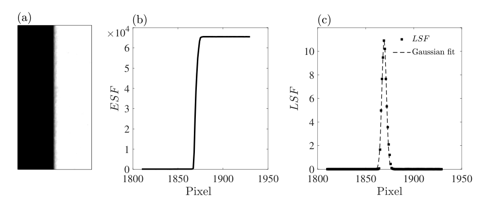
The resolving limit of the Rayleigh scattering measurements was the larger of the laser sheet thickness and the resolving limit of imaging obtained from a USAF 1951 target plate. To this end, a small window of a USAF 1951 target plate, with a sample shown in Fig. 1(a), was used. Then, the Edge Spread Function (ESF), which is the vertically-averaged intensity, versus the horizontal axis (in pixels) perpendicular to the edge was obtained and presented in Fig. 1(b). The derivative of ESF with respect to the horizontal axis is referred to as the Line Spread Function (LSF), which is presented in Fig. 1(c). A Gaussian variation was fit to the LSF, with this fit shown by the dotted curve in the figure. The Full Width at Half Maximum (FWHM) of the Gaussian fit was calculated and was approximately $198\,\mathrm{\tcmu m}$, which is smaller than the laser sheet thickness; and as a result, the resolving limit of our imaging was $216\,\mathrm{\tcmu m}$. In our earlier study Mohammadnejad and Kheirkhah (2024), the normalized energy and dissipation spectra of the temperature fluctuations was used and it was discussed that a spatial resolution of at least $314\,\mathrm{\tcmu m}$ is required to resolve the temperature fluctuations. This resolving limit is larger than the resolution of our Rayleigh scattering measurements.

A summary of the examined test conditions is presented in Table 1. In the table, the generic forms of U$X$F$Y$H$Z$P2 and U$X$F$Y$H$Z$AT are used to identify the test conditions for which two perforated plates or the active turbulence generator were used, respectively. In the symbols used for identifying the test conditions, $X$ and 0.$Y$ are the examined mean bulk flow velocity ($U$) and the fuel-air equivalence ratio ($\phi$), respectively. $Z$ is the volumetric percentage of the hydrogen-enrichment ($\mathrm{H_{2}}\%$). In the table, $L$ is the integral length scale and is estimated using the auto-correlation of the velocity data, with the details of the calculation provided in Mohammadnejad et al. (2022). The Taylor and Kolmogorov length scales were obtained using $l_{\mathrm{T}}=LRe^{-1/2}_{\mathrm{T}}$ and $\eta=LRe^{-3/4}_{\mathrm{T}}$, respectively. The turbulent Reynolds number is estimated from $Re_{\mathrm{T}}=u^{\prime}L/\nu$, with $u^{\prime}$ and $\nu$ being the RMS velocity fluctuations of the background turbulent cold flow and the reactants kinematic viscosity at 300 K, respectively. In Table 1, $Da=(u^{\prime}/S_{\mathrm{L,0}})^{-1}(L/\delta_{\mathrm{L}})$ and $Ka=(u^{\prime}/S_{\mathrm{L,0}})^{3/2}(L/\delta_{\mathrm{L}})^{-1/2}$ are the Damköhlder and Karlovitz numbers, respectively, with $\delta_{\mathrm{L}}$ being the laminar flame thickness. The unstretched laminar flame speed was calculated from the Cantera Goodwin et al. () simulations of one-dimensional freely propagating flames for the examined fuel and air mixtures and using GRI-Mech 3.0 Smith et al. (1999). The laminar flame thickness was estimated from $\delta_{\mathrm{L}}=(\lambda/c_{\mathrm{P}})/(\rho_{\mathrm{u}}S_{\mathrm{L,0}})$. In this calculation and similar to past studies Mohammadnejad et al. (2020); Driscoll et al. (2020); Mohammadnejad et al. (2021), the reactants density ($\rho_{\mathrm{u}}$) was estimated at 300 K, while the reactants thermal conductivity ($\lambda$) and heat-capacity-at-constant-pressure ($c_{\mathrm{P}}$) were both evaluated at 1500 K, using Mathur et al. (1967). For the combination of the examined $\phi$ and $\mathrm{H_{2}}\%$, the effective Lewis number of the examined methane-air and hydrogen-enriched methane air flames were calculated in Mohammadnejad and Kheirkhah (2024) and are about 1.0 and 0.8, respectively. It is important to note that, while the combination of $\phi$ and $\mathrm{H_{2}\%}$ in the present study is such that the Lewis number is rather close to unity, both $S_{\mathrm{L,0}}$ and $\delta_{\mathrm{L}}$ change notably. Specifically, $S_{\mathrm{L,0}}$ and $\delta_{\mathrm{L}}$ are 0.19 m/s and 0.33 mm for the examined methane-air flames and 0.08 m/s and 0.89 mm for the hydrogen-enriched methane air flames. Given these values and the characteristics of the examined background turbulent flow, the turbulent methane-air premixed flames featured $1.7\leq Ka\leq 5.8$; and, the turbulent hydrogen-enriched methane-air flames featured $11.2\leq Ka\leq 34.5$, as listed in Table 1. It is important to note that $\delta_{\mathrm{L}}$ is used for calculating several non-dimensional parameters, e.g., $Ka$ and $Da$ as listed in Table 1 of the present study and similar to past investigations reviewed in Driscoll et al. (2020). Compared to $\delta_{\mathrm{L}}$, however, $\delta_{\mathrm{th}}$ is used for normalizing the LES filter size and estimating several parameters relevant to Eq. (3), e.g., $Ka_{\Delta}$ and $Da_{\Delta}$. The Cantera Goodwin et al. () simulations (with GRI-Mech 3.0 Smith et al. (1999)) of freely propagating flames were used to estimate $\delta_{\mathrm{th}}$, which was 0.66 mm and 1.29 mm for the examined methane-air and hydrogen-enriched methane-air flames, respectively.

The Rayleigh scattering images were used to obtain the gas temperature from Skiba et al. (2022)

In Eq. (4), “ref” stands for the reference condition, corresponding to air at $T_{\mathrm{ref}}=300~\mathrm{K}$. Considering the small standard deviation of the laser energy fluctuations (which was less than 1% of the mean value), $I_{\mathrm{i}}/I_{\mathrm{i,ref}}\approx 1$. In Eq. (4), $I_{\mathrm{R}}$ and $I_{\mathrm{R,ref}}$ represent the Rayleigh scattering signals for the reacting and reference conditions, respectively. Both $I_{\mathrm{R}}$ and $I_{\mathrm{R,ref}}$ were corrected for background and noise. In Eq. (4), $\sigma_{\mathrm{mix}}$ and $\sigma_{\mathrm{mix,ref}}$ are the Rayleigh scattering cross-sections of the reacting mixture and air at a laser excitation wavelength of 532 nm, respectively.

Equation (4) along with the Cantera Goodwin et al. () simulations of the corresponding laminar premixed freely propagating flames (with GRI-Mech 3.0 Smith et al. (1999)) were used to estimate the normalized Rayleigh scattering intensity $I_{\mathrm{R}}/I_{\mathrm{R,ref}}$. The correlations between gas temperature and the normalized Rayleigh scattering intensity were derived from these Cantera simulations and discussed for both fuel compositions in Mohammadnejad and Kheirkhah (2024). These correlations were used to determine coefficients of fitting relations, following the methodology in Skiba et al. (2022). The resulting fitted curves were then employed to obtain the temperature fields of the turbulent premixed flames. The relationship between gas temperature and $I_{\mathrm{R}}/I_{\mathrm{R,ref}}$ (obtained from Cantera simulations) was also examined for different stretch factors and chemical kinetic mechanisms. The results suggested that changing the stretch factor from 0.1 to 10 did not change the above relationship using either GRI-Mech 3.0 Smith et al. (1999) (as also reported in Mohammadnejad and Kheirkhah (2024)) or the FFCM-2 mechanism Zhang et al. (2023). The above analysis suggests that the relation between gas temperature and $I_{\mathrm{R}}/I_{\mathrm{R,ref}}$ is nearly insensitive to the stretch effects and the utilized chemical kinetic mechanisms for the mixtures examined in the present study.

The two-dimensional temperature fields were filtered using wavelet-based denoising, self-guided edge-preserving, and 5$\times$5 median-based filters to remove “salt and paper” noise, with an example of a temperature field presented in Fig. 2(a). The Rayleigh scattering Region-of-Interest (ROI) extended from $x=-35.0\,\mathrm{mm}$ to 35.0 mm and from $y=43.0\,\mathrm{mm}$ to 70.0 mm. The signal-to-noise ratio (SNR) of the temperature field was obtained via calculating the ratio of the RMS temperature fluctuations divided by the mean temperature inside a window of 1 mm$\times$1 mm in the products, similar to Trueba-Monje and Sutton (2023). Across the examined test conditions, the SNR varied between 100 and 150, with these values being comparable to those reported in past studies, see for example Trueba-Monje and Sutton (2023).

Assessment of the resolved and unresolved terms in Eq. (2) requires estimating the density, thermal diffusivity, and scalar dissipation rate. The Cantera Goodwin et al. () simulations (with GRI-Mech 3.0 Smith et al. (1999)) of the unstretched laminar premixed flames were used to obtain the relations between temperature and thermal diffusivity as well as temperature and density. Then, the temperature fields along with these relations were used to obtain the two-dimensional variations of $\alpha$ and $\rho$. For example, the variations of $\alpha$ and $\rho$ for the temperature field shown in Fig. 2(a) are presented in Figs. 2(b) and (c), respectively. The temperature fields were used to calculate the combustion progress variable and $(\nabla c)^{2}$. It is acknowledged that calculating the latter requires estimating $\partial c/\partial x$ and $\partial c/\partial y$ as well as the derivative of the progress variable with respect to the direction normal to the plane of Rayleigh scattering measurements. This last derivative was not available in the present study, and as such $(\nabla c)^{2}$ is approximated as $(\nabla c)^{2}\approx(\partial c/\partial x)^{2}+(\partial c/\partial y)^{2}$, with representative results corresponding to the temperature filed in Fig. 2(a) presented in Fig. 2(d). Such two-dimensional (2D) approximation of $(\nabla c)^{2}$ has implications for the assessment of the terms in the algebraic model in Eq. (3), with details discussed later in section 4. Finally, the thermal diffusivity and $(\nabla c)^{2}$, see those in Figs. 2(b) and (d), were used to calculate $N_{c}$. The scalar dissipation rate field corresponding to the results in Figs. 2(a–d) is shown in Fig. 2(e).

Several 2D fields, e.g., the scalar dissipation rate, density, and thermal diffusivity, were separately filtered using the Gaussian and the sharp cut-off box filters. For the Gaussian filtering method, $\Delta$ was the kernel size (i.e., the standard deviation of the Gaussian distribution) following the approach in past studies Langella et al. (2017); Dunstan et al. (2013); Gao et al. (2014); Schumann et al. (2026). For the box filtering method, the filtering kernel, i.e. $\kappa(\Delta)$, in 2D space was Chen et al. (2005)

where $\mathbf{x}-\mathbf{r}$ was the vector connecting the center of the filtering box (here filtering window) to an arbitrary point in the 2D space.

The results are grouped into two subsections. In the first subsection, the characteristics of the scalar dissipation rate along with its resolved and unresolved terms (see, Eq. (2)) are discussed. In the second subsection, the algebraic model and constituent terms (see, Eq. (3)) are assessed.

A sub-grid-scale closure for the scalar dissipation rate ($N_{c}$) modeling used in the Large Eddy Simulations of turbulent premixed flames was studied experimentally. This closure was originally proposed by Kolla et al. (2009) in the framework of Favre-averaged Navier Stokes and later extended to the LES framework by Dunstan et al. (2013). Our experiments were performed using the hotwire anemometry technique to characterize the background turbulent flow, and the Rayleigh scattering to measure the scalar dissipation rate. The fuel was either methane or a mixture of 60% (by volume) methane and 40% hydrogen. The Karlovitz number varied between 1.7 and 34.5. The experimentally obtained scalar dissipation rate fields were filtered using LES filter sizes that varied between 0.1 to 3.0 times the thermal thickness of the examined laminar flames as well as using Gaussian and box filtering methods.

The Probability Density Function (PDF) of the Favre-filtered scalar dissipation rate ($\widetilde{N_{c}}$) as well as those of the resolved ($\widetilde{\alpha}(\nabla\widetilde{c})^{2}$) and unresolved ($\widetilde{\epsilon_{c}}$) scalar dissipation rate became generally broader by increasing the LES filter size. The PDF of $\widetilde{\epsilon_{c}}$ was asymmetric and skewed towards positive values. Consistent with the above finding, the ratio of temporally and spatially averaged filtered scalar dissipation rate and its resolved term ($<\overline{\overline{\widetilde{N_{c}}}}>/<\overline{\overline{\widetilde{\alpha}(\nabla\widetilde{c})^{2}}}>$) increased to several folds with increasing the normalized filter size. This increase was more pronounced for the results obtained using the Gaussian filtering method. These observations suggested the importance of modeling the unresolved term for predicting $\widetilde{N_{c}}$.

The variation of the temporally averaged scalar dissipation rate ($\overline{\overline{\widetilde{\epsilon_{c}}}}$) versus the temporally averaged combustion progress variable ($\overline{\overline{\widetilde{c}}}$) followed a parabolic-like distribution. Motivated by this, the Joint Probability Density Function analysis was performed and it was shown $\overline{\overline{\widetilde{\epsilon_{c}}}}$ follows a nearly linear relation with $\overline{\overline{\widetilde{c}(1-\widetilde{c})}}$. The slopes of such relations were obtained and used to estimate the temporally and spatially averaged unresolved term. The summation of the resolved and modeled unresolved terms was calculated, and compared with the measured filtered scalar dissipation rate. It was obtained that the algebraic model yielded acceptable prediction of the filtered scalar dissipation rate with a maximum deviation from the measured values of about $11\%$. This deviation was generally more pronounced at the larger examined normalized filter sizes. This conclusion was consistent for both examined filtering methods.

Our experimental measurements were used to estimate a key parameter, $\beta_{c,\mathrm{3D}}$, in the algebraic model used for predicting the unresolved scalar dissipation rate. While, $\beta_{c,\mathrm{3D}}$ obtained from the experimental measurements was relatively large for the examined small Karlovitz number flames, $\beta_{c,\mathrm{3D}}$ was similar to those reported in past numerical investigations and for the examined flames with relatively large Karlovitz numbers. Specifically, increasing the Karlovitz number from 11.2 to 34.5 increased $\beta_{c,\mathrm{3D}}$ from about 5 to 9, which is similar to 7.5 reported in Langella et al. (2017). This finding was shown to be independent of the examined filter type. To our best knowledge, the present study experimentally demonstrated for the first time that the measured values of $\beta_{c,\mathrm{3D}}$ are similar to those obtained from the filtered DNS for other flame configurations and are independent of the examined filtering method. While the results of the present study experimentally demonstrated the suitability of the algebraic sub-grid-scale closure for modeling the scalar dissipation rate, our findings are limited to the capabilities of our measurement techniques and extent of the examined test conditions. Future work will aim at addressing these limitations.

Morteza Nahvi: Writing-review & editing, Writing-original draft, Visualization, Methodology, Investigation, Formal analysis, Data curation. Sina Kheirkhah: Writing-review & editing, Writing-original draft, Supervision, Resources, Project administration, Methodology, Investigation, Funding acquisition.

The authors are thankful for the financial support from Alberta Innovates–Hydrogen Center of Excellence (HCOE2), Natural Sciences and Engineering Research Council of Canada (RGPIN-2025-04887), and Canada Foundation for Innovation (37470).

References

- Selle et al. (2004) Selle, L., Lartigue, G., Poinsot, T., Koch, R., Schildmacher, K.-U., Krebs, W., Prade, B., Kaufmann, P., Veynante, D. Compressible large eddy simulation of turbulent combustion in complex geometry on unstructured meshes. Combust. Flame 137, 489–505 (2004)
- Jella et al. (2021) Jella, S., Kwong, W., Steinberg, A., Park, J., Lu, T., Bergthorson, J., Bourque, G. Attached and lifted flame stabilization in a linear array of swirl injectors. Proc. Combust. Inst. 38, 6279–6287 (2021)
- Pitsch (2006) Pitsch, H. Large-Eddy Simulation of turbulent combustion. Annu. Rev. Fluid Mech. 38, 453–482 (2006)
- Langella et al. (2017) Langella, I., Swaminathan, N., Gao, Y., Chakraborty, N. Large Eddy Simulation of premixed combustion: sensitivity to subgrid scale velocity modeling. Combust. Sci. Technol. 189, 43–78 (2017)
- Langella et al. (2016) Langella, I., Swaminathan, N., Williams, F., Furukawa, J. Large-Eddy Simulation of premixed combustion in the corrugated-flamelet regime. Combust. Sci. Tech. 188, 1565–1591 (2016)
- Lapenna et al. (2024) Lapenna, P.E., Remiddi, A., Molinaro, D., Indelicato, G., Creta, F. A-posteriori analysis of a data-driven filtered wrinkled flamelet model for thermodiffusively unstable premixed flames. Combust. Flame 259, 113126 (2024)
- Dunstan et al. (2013) Dunstan, T.D., Minamoto, Y., Chakraborty, N., Swaminathan, N. Scalar dissipation rate modelling for Large Eddy Simulation of turbulent premixed flames. Proc. Combust. Inst. 34, 1193–1201 (2013)
- Nilsson et al. (2019) Nilsson, T., Langella, I., Doan, N.A.K., Swaminathan, N., Yu, R., Bai, X.-S. A priori analysis of sub-grid variance of a reactive scalar using DNS data of high Ka flames. Combust. Theor. Model. 23, 885–906 (2019)
- Kasten et al. (2022) Kasten, C., Shin, J., Sandberg, R., Pfitzner, M., Chakraborty, N., Klein, M. Modeling subgrid-scale scalar dissipation rate in turbulent premixed flames using gene expression programming and deep artificial neural networks. Phys. Fluids 34 (2022)
- Proch et al. (2017) Proch, F., Domingo, P., Vervisch, L., Kempf, A.M. Flame resolved simulation of a turbulent premixed bluff-body burner experiment. Part I: Analysis of the reaction zone dynamics with tabulated chemistry. Combust. Flame 180, 321–339 (2017)
- Luo et al. (2021) Luo, K., Liu, R., Bai, Y., Attili, A., Pitsch, H., Bisetti, F., Fan, J. A-priori and a-posteriori studies of a direct moment closure approach for turbulent combustion using DNS data of a premixed flame. Proc. Combust. Inst. 38, 3003–3011 (2021)
- Wang et al. (2025) Wang, Y., Xu, C., Scarcelli, R. A-priori and a-posteriori studies of finite-rate chemistry based combustion models for turbulent spherical lean premixed hydrogen/air flames. Proc. Combust. Inst. 41, 105815 (2025)
- Berger et al. (2025) Berger, L., Attili, A., Gauding, M., Pitsch, H. LES combustion model for premixed turbulent hydrogen flames with thermodiffusive instabilities: a priori and a posteriori analysis. J. Fluid Mech. 1003, 33 (2025)
- Pope and Anand (1985) Pope, S., Anand, M. Flamelet and distributed combustion in premixed turbulent flames. Proc. Combust. Inst. 20, 403–410 (1985)
- Veynante and Vervisch (2002) Veynante, D., Vervisch, L. Turbulent combustion modeling. Prog. Energy Combust. Sci. 28, 193–266 (2002)
- Poinsot and Veynante (2005) Poinsot, T., Veynante, D. Theoretical and Numerical Combustion, 2nd edn. R.T. Edwards, Inc., Philadelphia, PA (2005)
- Cant (2011) Cant, S. RANS and LES modelling of premixed turbulent combustion. In: Echekki, T., Mastorakos, E. (eds.) Turbulent Combustion Modeling: Advances, New Trends and Perspectives, pp. 63–90. Springer, Dordrecht (2011)
- Colin et al. (2000) Colin, O., Ducros, F., Veynante, D., Poinsot, T. A thickened flame model for large eddy simulations of turbulent premixed combustion. Phys. Fluids 12, 1843–1863 (2000)
- Han et al. (2019) Han, W., Wang, H., Kuenne, G., Hawkes, E.R., Chen, J.H., Janicka, J., Hasse, C. Large eddy simulation/dynamic thickened flame modeling of a high Karlovitz number turbulent premixed jet flame. Proc. Combust. Inst. 37, 2555–2563 (2019)
- Hawkes et al. (2011) Hawkes, E.R., Sankaran, R., Chen, J.H. Estimates of the three-dimensional flame surface density and every term in its transport equation from two-dimensional measurements. Proc. Combust. Inst. 33, 1447–1454 (2011)
- Ho et al. (2023) Ho, J.Z., Jella, S., Talei, M., Bourque, G., Indlekofer, T., Dawson, J. Assessment of the LES-FGM framework for capturing stable and unstable modes in a hydrogen/methane fuelled premixed combustor. Combust. Flame 255, 112904 (2023)
- Moureau et al. (2009) Moureau, V., Fiorina, B., Pitsch, H. A level set formulation for premixed combustion LES considering the turbulent flame structure. Combust. Flame 156, 801–812 (2009)
- Gao et al. (2014) Gao, Y., Chakraborty, N., Swaminathan, N. Algebraic closure of scalar dissipation rate for large eddy simulations of turbulent premixed combustion. Combust. Sci. Technol. 186, 1309–1337 (2014)
- Pfitzner (2021) Pfitzner, M. A new analytic pdf for simulations of premixed turbulent combustion. Flow Turbul. Combust. 106, 1213–1239 (2021)
- Liu and Wang (2022) Liu, J., Wang, H. Machine learning assisted modeling of mixing timescale for LES/PDF of high-Karlovitz turbulent premixed combustion. Combust. Flame 238, 111895 (2022)
- Wang et al. (2022) Wang, X., Wei, J., Su, X., Zhou, H., Ren, Z. Investigation of reaction-induced subgrid scalar mixing in LES/FDF simulations of turbulent premixed flames. Phys. Rev. Fluids 7, 124603 (2022)
- Lysenko and Ertesvåg (2018) Lysenko, D.A., Ertesvåg, I.S. Reynolds-averaged, scale-adaptive and large-eddy simulations of premixed bluff-body combustion using the eddy dissipation concept. Flow Turbul. Combust. 100, 721–768 (2018)
- Bray (1979) Bray, K.N.C. The interaction between turbulence and combustion. Proc. Combust. Inst. 17, 223–233 (1979)
- Bray (1980, pp. 115–183) Bray, K.N.C. Turbulent Flows with Premixed Reactants. In P. A. Libby and F. A. Williams (Eds.). Turbulent Reacting Flows, Springer, Berlin, Heidelburg (1980, pp. 115–183)
- Kolla et al. (2009) Kolla, H., Rogerson, J.W., Chakraborty, N., Swaminathan, N. Scalar dissipation rate modeling and its validation. Combust. Sci. Technol. 181, 518–535 (2009)
- Schumann et al. (2026) Schumann, C.D., Massey, J.C., Liu, Y., Li, C.J., Tanaka, Y., Swaminathan, N. A priori and a posteriori analyses of differential and preferential diffusion in large eddy simulations of partially premixed hydrogen–air flames. Combust. Flame 283, 114537 (2026)
- Vreman et al. (2009) Vreman, A., Van Oijen, J., De Goey, L., Bastiaans, R. Subgrid scale modeling in Large-Eddy Simulation of turbulent combustion using premixed flamelet chemistry. Flow, Turbul. Combust. 82, 511–535 (2009)
- Kazbekov and Steinberg (2021) Kazbekov, A., Steinberg, A.M. Physical space analysis of cross-scale turbulent kinetic energy transfer in premixed swirl flames. Combust. Flame 229, 111403 (2021)
- Ranjan et al. (2016) Ranjan, R., Muralidharan, B., Nagaoka, Y., Menon, S. Subgrid-scale modeling of reaction-diffusion and scalar transport in turbulent premixed flames. Combust. Sci. Technol. 188, 1496–1537 (2016)
- Chakraborty and Swaminathan (2011) Chakraborty, N., Swaminathan, N. Effects of Lewis number on scalar variance transport in premixed flames. Flow Turbul. Combust. 87, 261–292 (2011)
- Ma et al. (2014) Ma, T., Gao, Y., Kempf, A.M., Chakraborty, N. Validation and implementation of algebraic LES modelling of scalar dissipation rate for reaction rate closure in turbulent premixed combustion. Combust. Flame 161, 3134–3153 (2014)
- Nguyen et al. (2009) Nguyen, P., Bruel, P., Reichstadt, S. An experimental database for benchmarking simulations of turbulent premixed reacting flows: Lean extinction limits and velocity field measurements in a dump combustor. Flow Turbul. Combust. 82, 155–183 (2009)
- Sjunnesson et al. (1992) Sjunnesson, A., Henrikson, P., Lofstrom, C. CARS measurements and visualization of reacting flows in a bluff body stabilized flame. In: 28th Joint Propulsion Conference and Exhibit, p. 3650 (1992)
- Ferrante et al. (2024) Ferrante, G., Chen, Z.X., Langella, I. Dynamic modelling of subgrid scalar dissipation rate in premixed and partially premixed flames with differential filter. Appl. Therm. Eng. 248, 123233 (2024)
- Chakraborty and Swaminathan (2007) Chakraborty, N., Swaminathan, N. Influence of the Damköhler number on turbulence-scalar interaction in premixed flames. II. Model development. Phys. Fluids 19, 045104 (2007)
- Pope (2001) Pope, S.B. Turbulent Flows. Cambridge University Press, Cambridge, UK (2001)
- Ferziger (1997) Ferziger, J.H. Large Eddy Simulation: An introduction and perspective. In: New Tools in Turbulence Modelling: LES Houches School, May 21–31, 1996, pp. 29–47. Springer, Berlin, Heidelberg (1997)
- Lilly (1966) Lilly, D. The representation of small-scale turbulence in numerical simulation experiments. NCAR Report (1966)
- Hernández-Pérez et al. (2011) Hernández-Pérez, F., Yuen, F., Groth, C., Gülder, Ö. LES of a laboratory-scale turbulent premixed bunsen flame using FSD, PCM-FPI and thickened flame models. Proc. Combust. Inst. 33(1), 1365–1371 (2011)
- Shahbazian (2015) Shahbazian, N. Subfilter scale combustion modelling for Large Eddy Simulation of turbulent premixed flames. PhD thesis, University of Toronto (2015)
- Soulopoulos et al. (2014) Soulopoulos, N., Hardalupas, Y., Taylor, A. Scalar dissipation rate measurements in a starting jet. Exp. Fluids 55, 1685 (2014)
- Stetsyuk et al. (2016) Stetsyuk, V., Soulopoulos, N., Hardalupas, Y., Taylor, A. Scalar dissipation rate statistics in turbulent swirling jets. Phys. Fluids 28, 075104 (2016)
- Masri et al. (2004) Masri, A.R., Kalt, P.A., Barlow, R.S. The compositional structure of swirl-stabilised turbulent nonpremixed flames. Combust. Flame 137, 1–37 (2004)
- Kaiser and Frank (2007) Kaiser, S.A., Frank, J.H. Imaging of dissipative structures in the near field of a turbulent non-premixed jet flame. Proc. Combust. Inst. 31, 1515–1523 (2007)
- Sutton and Driscoll (2013) Sutton, J.A., Driscoll, J.F. Measurements and statistics of mixture fraction and scalar dissipation rates in turbulent non-premixed jet flames. Combust. Flame 160, 1767–1778 (2013)
- O’young and Bilger (1997) O’young, F., Bilger, R. Scalar gradient and related quantities in turbulent premixed flames. Combust. Flame 109(4), 682–700 (1997)
- Trueba-Monje and Sutton (2023) Trueba-Monje, I., Sutton, J.A. Flame structure and broadening in turbulent premixed jet flames. Combust. Flame 251, 112676 (2023)
- Skiba et al. (2022) Skiba, A.W., Carter, C.D., Hammack, S.D., Driscoll, J.F. Premixed flames subjected to extreme levels of turbulence part II: Surface characteristics and scalar dissipation rates. Combust. Flame 239, 111703 (2022)
- Kamal et al. (2017) Kamal, M.M., Coriton, B., Zhou, R., Frank, J.H., Hochgreb, S. Scalar dissipation rate and scales in swirling turbulent premixed flames. Proc. Combust. Inst. 36, 1957–1965 (2017)
- Mohammadnejad and Kheirkhah (2024) Mohammadnejad, S., Kheirkhah, S. Effects of combustion progress variable and Karlovitz number on the scalar dissipation rate of turbulent premixed hydrogen-enriched methane–air flames: An experimental study. Combust. Flame 269, 113669 (2024)
- Mohammadnejad and Kheirkhah (2025) Mohammadnejad, S., Kheirkhah, S. Spectral characteristic of a scalar-dissipation-rate-based turbulent burning velocity. Phys. Rev. Fluids 10, 023201 (2025)
- Mohammadnejad et al. (2022) Mohammadnejad, S., Saca, L., Kheirkhah, S. A new compact active turbulence generator for premixed combustion: Non-reacting flow characteristics. Phys. Fluids 34, 105102 (2022)
- (58) Goodwin, D.G., Speth, R.L., Moffat, H.K., Weber, B.W. Cantera: An Object-oriented Software Toolkit for Chemical Kinetics, Thermodynamics, and Transport Processes, 2018. https://www.cantera.org. Version 2.4.0
- Smith et al. (1999) Smith, G.P., Golden, D.M., Frenklach, M., Moriarty, N.W., Eiteneer, B., Goldenberg, M., Bowman, C.T., Hanson, R.K., Song, S., Gardiner, W.C.J., Lissianski, V.V., Qin, Z. GRI-Mech 3.0 (1999). http://www.me.berkeley.edu/gri-mech/
- Mohammadnejad et al. (2020) Mohammadnejad, S., An, Q., Vena, P., Yun, S., Kheirkhah, S. Thick reaction zones in non-flamelet turbulent premixed combustion. Combust. Flame 222, 285–304 (2020)
- Driscoll et al. (2020) Driscoll, J.F., Chen, J.H., Skiba, A.W., Carter, C.D., Hawkes, E.R., Wang, H. Premixed flames subjected to extreme turbulence: Some questions and recent answers. Prog. Energy Combust. Sci. 76, 100802 (2020)
- Mohammadnejad et al. (2021) Mohammadnejad, S., An, Q., Vena, P., Yun, S., Kheirkhah, S. Contributions of flame thickening and extinctions to a heat release rate marker of intensely turbulent premixed hydrogen-enriched methane-air flames. Combust. Flame 231, 111481 (2021)
- Mathur et al. (1967) Mathur, S., Tondon, P., Saxena, S. Thermal conductivity of binary, ternary and quaternary mixtures of rare gases. Mol. Phys. 12, 569–579 (1967)
- Zhang et al. (2023) Zhang, Y., Dong, W., Vandewalle, L., Xu, R., Smith, G., Wang, H. Foundational Fuel Chemistry Model Version 2.0 (FFCM-2) (2023). https://web.stanford.edu/group/haiwanglab/FFCM2
- Chen et al. (2005) Chen, J., Katz, J., Meneveau, C. Implication of mismatch between stress and strain-rate in turbulence subjected to rapid straining and destraining on dynamic LES models. J. Fluids Eng. 127, 840–850 (2005)
- Ghosal et al. (1995) Ghosal, S., Lund, T.S., Moin, P., Akselvoll, K. A dynamic localization model for large-eddy simulation of turbulent flows. J. Fluid Mech. 286, 229–255 (1995)
- Steinberg and Driscoll (2010) Steinberg, A.M., Driscoll, J.F. Stretch-rate relationships for turbulent premixed combustion les subgrid models measured using temporally resolved diagnostics. Combust. Flame 157(7), 1422–1435 (2010)
- Chakraborty et al. (2013) Chakraborty, N., Kolla, H., Sankaran, R., Hawkes, E.R., Chen, J.H., Swaminathan, N. Determination of three-dimensional quantities related to scalar dissipation rate and its transport from two-dimensional measurements: Direct numerical simulation based validation. Proc. Combust. Inst. 34, 1151–1162 (2013)
- Lavoie et al. (2007) Lavoie, P., Djenidi, L., Antonia, R. Effects of initial conditions in decaying turbulence generated by passive grids. J. Fluid Mech. 585, 395–420 (2007)
- Hearst and Lavoie (2014) Hearst, R.J., Lavoie, P. Decay of turbulence generated by a square-fractal-element grid. J. Fluid Mech. 741, 567–584 (2014)
- Gao et al. (2015) Gao, Y., Chakraborty, N., Swaminathan, N. Dynamic closure of scalar dissipation rate for Large Eddy Simulations of turbulent premixed combustion: A direct numerical simulations analysis. Flow Turbul. Combust. 95(4), 775–802 (2015)