Hall conductance of dilute electrolytes from odd stochastic density functional theory

We consider a system of $N$ particles of charge $q$ and mass $m$, immersed in a fluid at temperature $T$, and subjected to an external fixed magnetic field $\bm{B}=B\accentset{\wedge}{z}$. We describe the motion of the particles by the Langevin equation

	$\displaystyle\dot{\bm{x}}_{i}$	$\displaystyle=\bm{v}_{i}$		(2a)
	$\displaystyle m\dot{\bm{v}}_{i}$	$\displaystyle=-\frac{\partial U}{\partial\bm{x}_{i}}+q\bm{v}_{i}\times{\bf B}-\gamma\bm{v}_{i}+\bm{\xi}_{i}(t)$		(2b)

where $\bm{x}_{i}$ and $\bm{v}_{i}$ are the position and velocity, respectively, of the $i$’th particle ($i=1,...,N$), $\gamma$ is a friction coefficient, and $\bm{\xi}_{i}$ is a Gaussian white noise vector with zero mean, $\langle\bm{\xi}_{i}(t)\rangle=0$, and correlations

$$\langle\xi_{i}^{\mu}(t)\xi_{j}^{\nu}(t^{\prime})\rangle=2\gamma k_{B}T\delta_{ij}\delta_{\mu\nu}\delta(t-t^{\prime}).$$

(3)

The potential $U$ includes both pairwise interactions between the particles and external potentials, and is given by $U(\bm{x}_{1},...,\bm{x}_{N})=\frac{1}{2}\sum_{i\neq j=1}^{N}V\left(|\bm{x}_{i}-\bm{x}_{j}|\right)+\sum_{i}V_{{\rm ext}}\left(\bm{x}_{i}\right).$ Collecting terms that depend on $\bm{v}_{i}$, Eq. (2b) can be written as

$$m\dot{\bm{v}}_{i}=-\frac{\partial U}{\partial\bm{x}_{i}}-\mathsf{M}^{-1}\bm{v}_{i}+\bm{\xi}_{i}\left(t\right)$$

(4)

where $\mathsf{M}$ is the $3\times 3$ matrix

$$\mathsf{M}\equiv\frac{1}{\gamma}\left(\begin{array}[]{ccc}1&-\frac{qB}{\gamma}&0\\ \frac{qB}{\gamma}&1&0\\ 0&0&1\end{array}\right)^{-1}.$$

(5)

The dimensionless parameter $\omega_{c}\tau=qB/\gamma$ appearing in $\mathsf{M}$ compares two time scales involving the mass of the particle: the velocity relaxation time scale $\tau$ and the inverse cyclotron frequency $\omega_{c}^{-1}$, respectively given by

$$\tau\equiv\frac{m}{\gamma}\qquad\text{and}\qquad\omega_{c}^{-1}\equiv\frac{m}{qB}.$$

(6)

This parameter measures how much the particle velocity is rotated by the magnetic field during one relaxation time (the same parameter controls the weak- and strong-field regimes of the Hall effect in the Drude model [6]). When $\omega_{c}\tau\ll 1$, friction relaxes the velocity before the magnetic field can substantially deflect it. This corresponds to the low $B$ regime where

$$\mathsf{M}=\frac{1}{\gamma}\left(\begin{array}[]{ccc}1&\omega_{c}\tau&0\\ -\omega_{c}\tau&1&0\\ 0&0&1\end{array}\right)+\mathcal{O}(B^{2}).$$

(7)

For $B=0$, this reduces to $\gamma^{-1}\mathsf{I}$. When $\omega_{c}\tau\gg 1$, the particle undergoes many cyclotron rotations before its velocity is significantly relaxed. This corresponds to the high $B$ regime where

$$\mathsf{M}=\frac{1}{\gamma}\left(\begin{array}[]{ccc}(\omega_{c}\tau)^{-2}&(\omega_{c}\tau)^{-1}&0\\ -(\omega_{c}\tau)^{-1}&(\omega_{c}\tau)^{-2}&0\\ 0&0&1\end{array}\right)+\mathcal{O}(B^{-3}),$$

(8)

reducing to $M_{\mu\nu}=\gamma^{-1}\delta_{\mu 3}\delta_{\nu 3}$ in the $B\to\infty$ limit. Hence, a strong magnetic field suppresses the motion perpendicular to $\bm{B}$, while leaving the parallel motion unaffected.

Conventions— Throughout the text, Greek indices $\mu,\nu,\rho,\sigma$ label spatial components, e.g. $\mu=1,2,3$, whereas Greek indices $\alpha,\beta,\gamma,\delta$ label particle species, e.g. positively and negatively charged ions (relevant in Sec. IV). Both types of indices may appear as either subscripts or superscripts, with no distinction implied by their position. Repeated spatial indices are summed over according to the Einstein summation convention. Species indices, in contrast, are not summed over unless the summation is written explicitly. Vectors are denoted by bold symbols and matrices by sans-serif symbols. Their components are written in ordinary italic font, e.g. $\bm{x}$ becomes $x_{\mu}$ and $\mathsf{M}$ becomes $M_{\mu\nu}$. The identity matrix is denoted by $\mathsf{I}$, with components $I_{\mu\nu}=\delta_{\mu\nu}$, and the superscript ^T denotes matrix transposition.

In view of the two time scales in Eq. (6), taking $m\to 0$ is equivalent to saying that both $\tau$ and $\omega_{c}^{-1}$ are small compared to any other relevant time scale (e.g. given by $U$), yet $\omega_{c}\tau$ is held fixed. To assess whether this assumption is fulfilled, consider as an example standard salts such as $\rm NaCl$ in water at room temperature. In this case, $\tau\sim 10^{-2}\,\mathrm{ps}$ and $\omega_{c}^{-1}\sim 10^{5}\,\mathrm{ps}/B[\mathrm{T}]$ [62]. The Debye time $\tau_{D}=\lambda_{D}^{2}\gamma/k_{B}T$ (where $\lambda_{D}$ is the screening length) gives an order of magnitude of the timescales associated to electrostatic interactions in the solution [11]. Since $\tau_{D}\sim 100\,\mathrm{ps}/{c}[\mathrm{M}]$, $\tau\ll\tau_{D}$ is easily satisfied in most cases, yet $\omega_{c}^{-1}\ll\tau_{D}$ is restricted to very dilute solutions or strong magnetic fields. When the system is not in the low mass limit, one should retain both Eqs. (2a) and (2b). In contrast, in the low mass limit, we can eliminate $\bm{v_{i}}$ to get an equation on $\bm{x}_{i}$ only, simplifying the subsequent calculations.

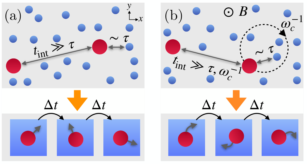
Intuitively, the low mass limit means that while the time over which a single particle loses its momentum is very small, so is the time it takes this particle to complete a full cyclotron orbit without the solvent (Fig. 1). Hence, on average, the particle performs a finite fraction of the circular motion before resetting (the exact fraction depends on the ratio $\tau/\tau_{c}$). Finally, note that taking the high $\gamma$ limit, rather than the low mass limit, would yield $\omega_{c}\tau\to 0$ and $\mathsf{M}\to\gamma^{-1}\mathsf{I}$, eliminating any signature of the magnetic field. Since we are interested in the effects of the magnetic field, the low mass limit is therefore the appropriate one here.

At first sight, one might expect the low-mass limit of Eq. (2) to be obtained simply by neglecting the inertial term. However, as shown in Ref. [32], this limit is more subtle (see Fig. 2). In the low-mass limit, Eq. (2) reduces to

$$\dot{\bm{x}}_{i}=-\mathsf{M}\frac{\partial U}{\partial\bm{x}_{i}}+\bm{\eta}_{i}\left(t\right)$$

(9)

with $\bm{\eta}_{i}$ being a nonwhite Gaussian vector with zero mean and correlations

	$\displaystyle\langle\bm{\eta}_{i}(t)\bm{\eta}_{j}^{\mathsf{T}}(t^{\prime})\rangle$	$\displaystyle=\delta_{ij}\mathsf{C}(t-t^{\prime})$		(10a)
with
	$\displaystyle\!\!\mathsf{C}(u)\equiv\lim_{m\to 0}\frac{k_{B}T}{m}e^{-\frac{\gamma|u|}{m}}$	$\displaystyle\begin{pmatrix}\cos(\frac{qB}{m}u)&\sin(\frac{qB}{m}u)&0\\[2.84544pt] -\sin(\frac{qB}{m}u)&\cos(\frac{qB}{m}u)&0\\[2.84544pt] 0&0&1\end{pmatrix}$		(10b)
	$\displaystyle=\lim_{\begin{subarray}{c}\tau\to 0\\ \omega_{c}\tau=\mathrm{const}\end{subarray}}\frac{k_{B}T}{\gamma\tau}e^{-\frac{|u|}{\tau}}$	$\displaystyle\begin{pmatrix}\cos(\omega_{c}u)&\sin(\omega_{c}u)&0\\[2.84544pt] -\sin(\omega_{c}u)&\cos(\omega_{c}u)&0\\[2.84544pt] 0&0&1\end{pmatrix}$		(10c)

The limit in Eq. (10b) can be expressed as [32]

$$\mathsf{C}(u)=k_{B}T\left[\mathsf{M}\delta_{+}\left(u\right)+\mathsf{M}^{\mathsf{T}}\delta_{-}\left(u\right)\right]$$

(11)

where $\delta_{+}(u)$ and $\delta_{-}(u)$ are variants of the Dirac delta function restricted to the nonnegative and nonpositive real lines, respectively, so they vanish when $u\neq 0$ and satisfy $\int_{0}^{\infty}\delta_{+}(u){\rm d}u=\int_{-\infty}^{0}\delta_{-}(u){\rm d}u=1$ and $\int_{0}^{\infty}\delta_{-}(u){\rm d}u=\int_{-\infty}^{0}\delta_{+}(u){\rm d}u=0$.

Our goal in the next two subsections is to find a density-field description of Eqs. (9–10), analogous to the Dean-Kawasaki equation, which is a density-field description of the standard overdamped Langevin equation with white noise.

While we focus on charged particles under magnetic field, Eq. (2) has been used to model odd-diffusive fluids [3, 68, 67], and therefore the following derivation applies to such systems as well in the low mass limit. Moreover, Eq. (9) describes chiral active particles [26] under certain limits and mappings specified in Appendix A. Hence, the odd Dean-Kawasaki equation we derive can also be extended to describe such models (see Appendix A for details).

The standard derivation of the Dean-Kawasaki equation starts from the overdamped Langevin equation [36]. However, it relies on Ito calculus, applicable for white noise only. Since in our case the the low-mass limit has a nonwhite noise (Eq. (10)), it is not obvious how to follow the same path of the original derivation. Instead, we derive a fluctuating hydrodynamic equation for the number density field and momentum density field, using a formalism introduced in Ref. [98], and take the low-mass limit at the density field level (see Fig. 2).

The number density field is defined as

$$n(\bm{x},t)\equiv\sum_{i}\delta(\bm{x}-\bm{x}_{i}(t))$$

(12)

and the momentum density field as

$$\bm{g}(\bm{x},t)\equiv\sum_{i}m\bm{v}_{i}(t)\delta(\bm{x}-\bm{x}_{i}(t)).$$

(13)

Taking the time derivative of Eq. (12) and using Eq. (2), we obtain

	$\displaystyle\partial_{t}n(\bm{x},t)$	$\displaystyle=-\sum_{i}\bm{v}_{i}(t)\cdot\bm{\nabla}\delta(\bm{x}-\bm{x}_{i}(t))$
		$\displaystyle=-\frac{1}{m}\bm{\nabla}\cdot\bm{g}(\bm{x},t)$		(14)

Similarly, taking the time derivative of Eq. (13) we obtain

	$\displaystyle\partial_{t}\bm{g}(\bm{x},t)$	$\displaystyle=m\sum_{i}\dot{\bm{v}}_{i}\delta(\bm{x}-\bm{x}_{i}(t))$		(15)
		$\displaystyle-m\sum_{i}\bm{v}_{i}(\dot{\bm{x}}_{i}(t)\cdot\bm{\nabla}\delta(\bm{x}-\bm{x}_{i}(t)))$
		$\displaystyle=-\frac{1}{m}\mathsf{M}^{-1}\bm{g}-n\nabla\frac{\delta U}{\delta n}-\bm{\nabla}\cdot\mathsf{G}+\bm{\xi}$

where, in the last step, we used the relation ${\sum_{i}\frac{\partial U}{\partial\bm{x}_{i}}\delta(\bm{x}-\bm{x}_{i}(t))=n(\bm{x},t)\nabla\frac{\delta U}{\delta n(\bm{x},t)}}$ that arise from the expression

$${U=\frac{1}{2}\int{\rm d}\bm{x}{\rm d}\bm{x}^{\prime}n(\bm{x})V(\bm{x}-\bm{x}^{\prime})n(\bm{x}^{\prime})+\int n(\bm{x})V_{{\rm ext}}(\bm{x})}\text{d}\bm{x}$$

of the potential, and defined

	$\displaystyle\bm{\xi}(\bm{x},t)\equiv$	$\displaystyle\sum_{i}\bm{\xi}_{i}(t)\delta(\bm{x}-\bm{x}_{i}(t))$		(16a)
	$\displaystyle\mathsf{G}(\bm{x},t)\equiv\,$	$\displaystyle m\sum_{i}\bm{v}_{i}(t)\bm{v}^{\mathsf{T}}_{i}(t)\delta(\bm{x}-\bm{x}_{i}(t)).$		(16b)

Using Eq. (3) and following the same argument as the original derivation by Dean [36], namely that $\delta(\bm{x}-\bm{x}_{i})\delta(\bm{x}^{\prime}-\bm{x}_{i})=\delta(\bm{x}-\bm{x}^{\prime})\delta(\bm{x}-\bm{x}_{i})$, we find the new noise correlations to be

$\displaystyle\!\!\!\!\langle\bm{\xi}(\bm{x},t)\bm{\xi}^{\mathsf{T}}(\bm{x}^{\prime},t^{\prime})\rangle$

$\displaystyle=2\gamma k_{B}Tn(\bm{x},t)\delta(\bm{x}-\bm{x}^{\prime})\delta(t-t^{\prime})\mathsf{I}$

(17)

Following Ref. [98], we assume that

$$\delta(\bm{x}_{i}(t)-\bm{x}_{j}(t))=\delta(\bm{x}_{i}(t)-\bm{x}_{j}(t))\delta_{ij}$$

(18)

which is valid if the particles do not overlap (this is justified if the potential has a repulsive core but also in the dilute limit or simply by considering point-like particles in three dimensions). We then insert a representation of unity in terms of delta functions, which yields

	$\displaystyle G^{\mu\nu}$	$\displaystyle=m\sum_{i}v_{i}^{\mu}(t)v_{i}^{\nu}(t)\delta(\bm{x}-\bm{x}_{i}(t))\frac{\sum\limits_{j}\delta(\bm{x}-\bm{x}_{j}(t))}{\sum\limits_{k}\delta(\bm{x}-\bm{x}_{k}(t))}$
		$\displaystyle=\frac{m}{n}\sum_{i}v_{i}^{\mu}(t)\delta(\bm{x}-\bm{x}_{i}(t))\sum_{j}v_{j}^{\nu}(t)\delta(\bm{x}-\bm{x}_{j}(t))$
		$\displaystyle=\frac{g_{\nu}(\bm{x},t)g_{\nu}(\bm{x},t)}{m\,n(\bm{x},t)}.$		(19)

In going from the first line to the second, we used the definition of $n$, Eq. (12), together with the relation (18); from the second line to the third, we used the definition of $g$, Eq. (13). Finally, we find that the evolution of the momentum density field is given by

$$\partial_{t}g_{\mu}(\bm{x},t)=-\frac{(\mathsf{M}^{-1})_{\mu\nu}g_{\nu}}{m}-n\partial_{\mu}\frac{\delta U}{\delta n}-\partial_{\nu}\frac{g_{\mu}g_{\nu}}{m\,n}+\xi_{\mu}.$$

(20)

Next, we eliminate $\bm{g}$ by taking the low mass limit. In the following derivation it will be useful to work with the dimensionless matrix

$$\mathsf{\Gamma}\equiv\gamma^{-1}\mathsf{M}^{-1}=\left(\begin{array}[]{ccc}1&-\frac{qB}{\gamma}&0\\ \frac{qB}{\gamma}&1&0\\ 0&0&1\end{array}\right).$$

(21)

The use of $\mathsf{\Gamma}$ instead of $\mathsf{M}$ is restricted to this subsection. Equation (20) can be formally solved as

$$\frac{1}{\tau}\bm{g}(\bm{x},t)=\bm{\Upsilon}+\bm{\Xi}+\bm{\Pi}$$

(22)

where

	$\displaystyle\bm{\Upsilon}(\bm{x},t)$	$\displaystyle\equiv-\frac{1}{\tau}\int\limits_{-\infty}^{t}{\rm d}se^{-\frac{\mathsf{\Gamma}(t-s)}{\tau}}n(\bm{x},s)\bm{\nabla}\frac{\delta U}{\delta n(\bm{x},s)}$		(23a)
	$\displaystyle\bm{\Xi}(\bm{x},t)$	$\displaystyle\equiv\frac{1}{\tau}\int\limits_{-\infty}^{t}{\rm d}se^{-\frac{\mathsf{\Gamma}(t-s)}{\tau}}\bm{\xi}(\bm{x},s)$		(23b)
	$\displaystyle\bm{\Pi}(\bm{x},t)$	$\displaystyle\equiv-\frac{1}{\tau^{2}\gamma}\int\limits_{-\infty}^{t}{\rm d}se^{-\frac{\mathsf{\Gamma}(t-s)}{\tau}}\bm{\nabla}\cdot\frac{\bm{g}(\bm{x},s)\bm{g}^{\mathsf{T}}(\bm{x},s)}{n(\bm{x},s)}$		(23c)

and the matrix elements of $e^{-\mathsf{\Gamma}u/\tau}$ are

$$e^{-\mathsf{\Gamma}u/\tau}=e^{-u/\tau}\left(\begin{array}[]{ccc}\cos\left(\omega_{c}u\right)&\sin\left(\omega_{c}u\right)&0\\ -\sin\left(\omega_{c}u\right)&\cos\left(\omega_{c}u\right)&0\\ 0&0&1\end{array}\right).$$

(24)

This is an implicit solution because $\bm{\Pi}$ depends on $\bm{g}$.

The new noise, $\bm{\Xi}$, is a Gaussian noise with zero mean, and substituting Eq. (17) its correlations are,

	$\displaystyle\langle\bm{\Xi}(\bm{x},t)\bm{\Xi}^{\mathsf{T}}(\bm{x}^{\prime},t^{\prime})\rangle$	$\displaystyle=\frac{2\gamma k_{B}T\delta(\bm{x}-\bm{x}^{\prime})}{\tau^{2}}$		(25)
		$\displaystyle\times\int\limits_{-\infty}^{t_{<}}{\rm d}s\,e^{-\mathsf{\Gamma}\frac{(t-s)}{\tau}}n(\bm{x},s)e^{-\mathsf{\Gamma}^{\mathsf{T}}\frac{(t^{\prime}-s)}{\tau}}$

where $t_{<}\equiv{\min(t,t^{\prime})}$. Using trigonometric identities and the relation ${t+t^{\prime}-2s=\left|t-t^{\prime}\right|+2(t_{<}-s)}$ we obtain

	$\displaystyle\langle\bm{\Xi}(\bm{x},t)\bm{\Xi}^{\mathsf{T}}(\bm{x}^{\prime},t^{\prime})\rangle$	$\displaystyle=\frac{2\gamma^{2}}{\tau}\delta(\bm{x}-\bm{x}^{\prime})\mathsf{C}_{m}(t-t^{\prime})$
		$\displaystyle\times\int\limits_{-\infty}^{t_{<}}{\rm d}s\,e^{-\frac{2(t_{<}-s)}{\tau}}n(\bm{x},s)$		(26)

where

$$\mathsf{C}_{m}(u)\equiv\frac{k_{B}T}{\gamma\tau}e^{-\left|u\right|/\tau}\left(\begin{array}[]{ccc}\cos\left(\omega_{c}u\right)&\sin\left(\omega_{c}u\right)&0\\ -\sin\left(\omega_{c}u\right)&\cos\left(\omega_{c}u\right)&0\\ 0&0&1\end{array}\right).$$

(27)

We now use the fact that $n(\bm{x},t)$ varies only weakly over the fast time scales $\tau$ and $\omega_{c}^{-1}$ (unlike $\bm{g}(\bm{x},t)$). Hence, in the low mass limit, $\frac{1}{\tau}\int\limits_{-\infty}^{t_{<}}{\rm d}s\,e^{-\frac{2(t_{<}-s)}{\tau}}n(\bm{x},s)\to\frac{1}{2}n(\bm{x},t_{<})$. Moreover, as was proven in Ref. [32], in the low mass limit $\lim_{m\to 0}\mathsf{C}_{m}(u)=\mathsf{C}(u)$ (with $\mathsf{C}$ given by Eq. (11)), so we obtain

$$\!\!\lim_{m\to 0}\langle\bm{\Xi}(\bm{x},t)\bm{\Xi}^{\mathsf{T}}(\bm{x}^{\prime},t^{\prime})\rangle=\gamma^{2}n(\bm{x},t)\delta(\bm{x}-\bm{x}^{\prime})\mathsf{C}(t-t^{\prime}).$$

(28)

Note that we have assumed Ito prescription. For a different prescription, one has to integrate Eq. (14) over a time $\Delta t\gg\tau,\omega_{c}^{-1}$ and evaluate the multiplicative part of the noise that depends on $n$ at $t^{*}$ where $t<t^{*}<t+\Delta t$ and $\Delta t$ (see Ref. [82] for details).

To evaluate $\bm{\Upsilon}$, we notice that for $u>0$, $e^{-\mathsf{\Gamma}u/\tau}=\frac{\gamma\tau}{k_{B}T}\mathsf{C}_{m}(u)$ (compare Eq. (24) and (27)). Hence, for a function $h(t)$ that varies on time scale much larger than both $\tau$ and $\omega_{c}^{-1}$,

	$\displaystyle\lim_{m\to 0}\frac{1}{\tau}\int_{-\infty}^{t}\!\!\!{\rm d}s\,e^{-\frac{\mathsf{\Gamma}(t-s)}{\tau}}h(s)$	$\displaystyle=\frac{\gamma}{k_{B}T}\int_{-\infty}^{t}\!\!\!{\rm d}s\,\mathsf{C}(t-s)h(s)$
		$\displaystyle=h(t)\mathsf{\Gamma}^{-1},$		(29)

hence we obtain

$$\lim_{m\to 0}\bm{\Upsilon}(\bm{x},t)=-n(\bm{x},t)\mathsf{\Gamma}^{-1}\bm{\nabla}\frac{\delta U}{\delta n(\bm{x},t)}.$$

(30)

We are left with evaluating Eq. (23c) in the low-mass limit. As is pointed out in Ref. [98], the lowest order contribution to $\bm{g}$ in powers of $\tau$ (or $m$), as given in Eq. (22), is

$$\bm{g}(\bm{x},s)\approx\tau\bm{\Xi}.$$

(31)

Indeed, $\bm{\Xi}(\bm{x},t)\sim\tau^{-1/2}$, as follows from $\langle\bm{\Xi}(\bm{x},t)\bm{\Xi}^{\mathsf{T}}(\bm{x},t)\rangle\sim\tau^{-1}$ (see Eq. (27)), whereas $\bm{\Upsilon}(\bm{x},t)\sim\tau^{0}$. As we show below, the remaining contribution is also self-consistently of order $\bm{\Pi}(\bm{x},t)\sim\tau^{0}$. Hence, we can approximate $\bm{\Pi}$ to leading order in $\tau$ as

$$\bm{\Pi}(\bm{x},t)\approx-\frac{1}{\gamma}\int\limits_{-\infty}^{t}{\rm d}se^{-\frac{\mathsf{\Gamma}(t-s)}{\tau}}\bm{\nabla}\cdot\frac{\bm{\Xi}(\bm{x},s)\bm{\Xi}^{\mathsf{T}}(\bm{x},s)}{n(\bm{x},s)}.$$

(32)

Note that the right hand side of Eq. (32) is stochastic. However, it suffices to retain only its average (deterministic) contribution, since the fluctuating part is subdominant to $\bm{\Xi}$ (when integrated over a time interval $\Delta t$ it scales as $\Delta t$, while $\Xi$ scales with $\Delta t^{1/2}$). Following Eq. (26), the average of $\bm{\Xi}(\bm{x},s)\bm{\Xi}^{\mathsf{T}}(\bm{x},s)$ is

	$\displaystyle\langle\bm{\Xi}(\bm{x},s)\bm{\Xi}^{\mathsf{T}}(\bm{x},s)\rangle$	$\displaystyle=\frac{2\gamma k_{B}T}{\tau^{2}}\mathsf{I}\delta(\bm{x}-\bm{x})$
		$\displaystyle\times\int\limits_{-\infty}^{s}{\rm d}s^{\prime}\,e^{-\frac{2(s-s^{\prime})}{\tau}}n(\bm{x},s^{\prime})$		(33)

where we used $\mathsf{C}_{m}(0)=k_{B}T/(\gamma\tau)$ (see Eq. (27)). While this expression appears problematic because of the $\delta(\bm{x}-\bm{x})$, we follow Ref. [98] and use the relation $n(\bm{x},t)^{2}=\delta(\bm{x}-\bm{x})n(\bm{x},t)$ derived from substituting the definition in Eq. (12) and using Eq. (18) (for more rigorous justification see Ref. [98]). We obtain, to leading order in $\tau$,

	$\displaystyle\bm{\Pi}(\bm{x},t)$	$\displaystyle=-\frac{2k_{B}T}{\tau^{2}}\bm{\nabla}\int\limits_{-\infty}^{t}{\rm d}se^{-\frac{\mathsf{\Gamma}(t-s)}{\tau}}$
		$\displaystyle\times\frac{1}{n(\bm{x},s)}\int\limits_{-\infty}^{s}{\rm d}s^{\prime}\,e^{-\frac{2(s-s^{\prime})}{\tau}}n(\bm{x},s^{\prime})^{2}$		(34)

which, in the $m\to 0$ limit, becomes

$$\lim_{m\to 0}\bm{\Pi}(\bm{x},t)=-k_{B}T\mathsf{\Gamma}^{-1}\bm{\nabla}n(\bm{x},t).$$

(35)

Inserting the results of Eqs. (28), (30) and (35) into Eq. (22) we obtain

	$\displaystyle\partial_{t}n(\bm{x},t)$	$\displaystyle=-\bm{\nabla}\cdot\bm{J}$		(36a)
	$\displaystyle\bm{J}=-k_{B}$	$\displaystyle T\mathsf{M}\bm{\nabla}n-n\mathsf{M}\bm{\nabla}\frac{\delta U}{\delta n}+\bm{\chi}(\bm{x},t)$		(36b)
	$\displaystyle\langle\bm{\chi}(\bm{x},t)\bm{\chi}$	$\displaystyle(\bm{x}^{\prime},t^{\prime})^{\mathsf{T}}\rangle=n(\bm{x},t)\delta(\bm{x}-\bm{x}^{\prime})\mathsf{C}(t-t^{\prime})$		(36c)

where $\bm{J}(\bm{x},t)=\bm{g}(\bm{x},t)/m$ is the density current and we defined the rescaled Gaussian noise $\bm{\chi}\equiv\bm{\Xi}/\gamma$ with $\langle\bm{\chi}\rangle=0$. Equation (36) constitutes the odd Dean-Kawasaki equation for particles under a Lorentz force. A modified version for chiral active particles is presented in Appendix A.

We conclude this section by demonstrating how the odd Dean-Kawasaki equation can be used to calculate a transport coefficient in a simple setup. Readers interested in the Hall conductivity can directly skip to Sec. IV. Consider a collection of particles subject to an external force that is fixed and uniform, $\bm{F}=F_{0}\accentset{\wedge}{n}$. The system’s response can be characterized by the collective mobility tensor $\mathsf{L}$, which relates the average density current to the external force through

$$\langle\bm{J}\rangle=\mathsf{L}\,\bm{F}.$$

(37)

We can derive $\mathsf{L}$ from the odd Dean-Kawasaki equation using either direct response or Green-Kubo relation, as described below. For simplicity, we first consider the case of noninteracting particles ($V=0$); the more complicated case with $V\neq 0$, together with a generalization of Eq. (37) to a spatiotemporal force, is treated in Appendix B. Additionally, the collective mobility of chiral active particles is derived from a modified odd Dean-Kawasaki equation in Appendix C. We show that, in this case, the Green-Kubo relation is no longer valid.

In the following, we derive three different formulas for the conductivity, based on (i) direct response, (ii) the Green-Kubo relation, and (iii) a hybrid fluctuation-dissipation relation.

References

• [1] M. Abbes, R. Gérard, P. Gérard, M. Meton, and E.J. Picard (1980) Effet hall dans des solutions électrolytiques de concentration variable. Journal de Physique Lettres 41 (23), pp. 575–580. External Links: Document, ISSN 0302-072X Cited by: §V.
• [2] M. Abbes, R. Gérard, P. Gérard, M. Meton, and E.J. Picard (1982) Effet hall de chlorures et d’iodures en solutions diluées dans le méthanol et dans l’eau. Journal de Physique Lettres 43 (5), pp. 127–132. External Links: Document, ISSN 0302-072X Cited by: §V.
• [3] I. Abdoli, R. Wittmann, and H. Löwen (2026) Dynamical density functional theory for dense odd-diffusive fluids. The Journal of Physical Chemistry B 130 (17), pp. 4672–4682. External Links: Document, ISSN 1520-5207 Cited by: §I, §III.2.
• [4] R. M. Adar, T. Markovich, A. Levy, H. Orland, and D. Andelman (2018) Dielectric constant of ionic solutions: combined effects of correlations and excluded volume. The Journal of chemical physics 149 (5), pp. 054504. External Links: Document Cited by: §I, §V.
• [5] A. Altenberger and H. L. Friedman (1983) Theory of conductance and related isothermal transport coefficients in electrolytes. Journal of Chemical Physics 78 (6), pp. 4162–4173. External Links: Document Cited by: §I.
• [6] N. W. Ashcroft N. D. Mermin et al. (1976) Solid state physics. holt, rinehart and winston, new york London. Cited by: §III.1.
• [7] Y. Avni, R. M. Adar, D. Andelman, and H. Orland (2022) Conductivity of concentrated electrolytes. Physical Review Letters 128 (9), pp. 098002. External Links: Document Cited by: §I, §V.
• [8] Y. Avni, D. Andelman, and H. Orland (2022) Conductance of concentrated electrolytes: multivalency and the wien effect. The Journal of Chemical Physics 157 (15), pp. 154502. External Links: Document Cited by: §I.
• [9] Y. Avni, M. Fruchart, D. Martin, T. Khain, and V. Vitelli (2026) (To be published).. Cited by: §I, §II, §V.
• [10] Y. Avni, M. Fruchart, D. Martin, D. Seara, and V. Vitelli (2025) Dynamical phase transitions in the nonreciprocal ising model. Physical Review E 111 (3), pp. 034124. External Links: Document Cited by: §A.1.1.
• [11] M. Z. Bazant, K. Thornton, and A. Ajdari (2004) Diffuse-charge dynamics in electrochemical systems. Physical Review E—Statistical, Nonlinear, and Soft Matter Physics 70 (2), pp. 021506. External Links: Document Cited by: §III.2.
• [12] M.L. Belaya, M.V. Feigel’man, and V.G. Levadny (1986) Hydration forces as a result of non-local water polarizability. Chemical Physics Letters 126 (3-4), pp. 361–364. External Links: Document, ISSN 0009-2614 Cited by: §I, §V.
• [13] M. Bellissent, P. Gerard, C. Longevialle, M. Meton, M. Pich, and G. Morand (1971) Eperimental measurements of the hall effect in very dilute solutions. Journal of The Electrochemical Society 118 (12), pp. 1944. External Links: Document, ISSN 0013-4651 Cited by: §V.
• [14] A. Benois, M. Jardat, V. Dahirel, V. Démery, J. Agudo-Canalejo, R. Golestanian, and P. Illien (2023) Enhanced diffusion of tracer particles in nonreciprocal mixtures. Physical Review E 108 (5), pp. 054606. External Links: Document Cited by: §I.
• [15] O. Bernard, W. Kunz, P. Turq, and L. Blum (1992) Conductance in electrolyte solutions using the mean spherical approximation. The Journal of Physical Chemistry 96 (9), pp. 3833–3840. External Links: Document Cited by: §I.
• [16] H. Berthoumieux and F. Paillusson (2019) Dielectric response in the vicinity of an ion: a nonlocal and nonlinear model of the dielectric properties of water. The Journal of Chemical Physics 150 (9), pp. 094507. External Links: Document, ISSN 1089-7690 Cited by: §I, §V.
• [17] H. Berthoumieux, V. Démery, and A. C. Maggs (2024) Nonlinear conductivity of aqueous electrolytes: beyond the first wien effect. The Journal of Chemical Physics 161 (18), pp. 184504. External Links: Document, ISSN 1089-7690 Cited by: §I, §I, §V.
• [18] H. Berthoumieux, G. Monet, and R. Blossey (2021) Dipolar poisson models in a dual view. The Journal of Chemical Physics 155 (2), pp. 024112. External Links: Document, ISSN 1089-7690 Cited by: §I, §V.
• [19] R. Blossey and R. Podgornik (2022) Continuum theories of structured dielectrics. Europhysics Letters 139 (2), pp. 27002. External Links: Document, ISSN 1286-4854 Cited by: §I, §V.
• [20] R. Blossey and R. Podgornik (2022) Field theory of structured liquid dielectrics. Physical Review Research 4 (2), pp. 023033. External Links: Document, ISSN 2643-1564 Cited by: §I, §V.
• [21] J. O’M. Bockris and A. K. N. Reddy (1998) Modern electrochemistry 1: ionics. 2 edition, Kluwer Academic/Plenum Publishers, New York. External Links: ISBN 0-306-45554-4 Cited by: §I, §V.
• [22] S. Bonella, G. Ciccotti, and L. Rondoni (2014) Time reversal symmetry in time-dependent correlation functions for systems in a constant magnetic field. EPL (Europhysics Letters) 108 (6), pp. 60004. External Links: Document, ISSN 1286-4854 Cited by: Appendix D.
• [23] S. Bonella, A. Coretti, L. Rondoni, and G. Ciccotti (2017) Time-reversal symmetry for systems in a constant external magnetic field. Physical Review E 96 (1), pp. 012160. External Links: Document, ISSN 2470-0053 Cited by: Appendix D.
• [24] H. Brinkman (1956) Brownian motion in a field of force and the diffusion theory of chemical reactions. Physica 22 (1-5), pp. 29–34. External Links: Document Cited by: Figure 2.
• [25] Y. A. Budkov and N. N. Kalikin (2026) Hall effect in electrolyte solutions: self-consistent debye–hückel–onsager theory. The Journal of Chemical Physics 165 (6), pp. 064506. External Links: Document, ISSN 1089-7690 Cited by: §V.
• [26] L. Caprini, H. Löwen, and U. M. B. Marconi (2023) Chiral active matter in external potentials. Soft Matter 19 (33), pp. 6234–6246. External Links: Document Cited by: §A.1, §I, §III.2.
• [27] M. E. Cates and J. Tailleur (2013) When are active brownian particles and run-and-tumble particles equivalent? consequences for motility-induced phase separation. Europhysics Letters 101 (2), pp. 20010. External Links: Document Cited by: §A.2.
• [28] A. Chandra and B. Bagchi (1999) Ion conductance in electrolyte solutions. The Journal of chemical physics 110 (20), pp. 10024–10034. External Links: Document Cited by: §I.
• [29] V.R. Chechetkin and V.S. Lutovinov (1989) On the hall number in dilute electrolyte solutions. Molecular Physics 68 (4), pp. 979–981. External Links: Document, ISSN 1362-3028 Cited by: §V.
• [30] J. Chen, J. Ying, Y. Tian, Y. Xiao, and X. Yang (2024) Electrocatalysis under magnetic fields. Advanced Functional Materials 35 (8), pp. 2415660. External Links: Document, ISSN 1616-3028 Cited by: §V.
• [31] H. Chun and T. D. Chung (2015) Iontronics. Annual Review of Analytical Chemistry 8 (1), pp. 441–462. External Links: Document, ISSN 1936-1335 Cited by: §V.
• [32] H. Chun, X. Durang, and J. D. Noh (2018) Emergence of nonwhite noise in langevin dynamics with magnetic lorentz force. Physical Review E 97 (3), pp. 032117. External Links: Document Cited by: Appendix E, §II, Figure 2, §III.2, §III.2, §III.4.
• [33] H. Chun, Q. Gao, and J. M. Horowitz (2021) Nonequilibrium green-kubo relations for hydrodynamic transport from an equilibrium-like fluctuation-response equality. Physical Review Research 3 (4), pp. 043172. External Links: Document Cited by: §III.5.2.
• [34] P. B. Corkum and J. A. McLennan (1974) Green–kubo formulae for a plasma in an external magnetic field. Canadian Journal of Physics 52 (6), pp. 516–522. External Links: Document, ISSN 1208-6045 Cited by: Appendix D, §III.5.2.
• [35] D. S. Dean and H. Diamant (2026) Dielectric response as a source of viscosity in polar liquids. External Links: 2604.00262 Cited by: §I, §I, §V.
• [36] D. S. Dean (1996) Langevin equation for the density of a system of interacting langevin processes. Journal of Physics A: Mathematical and General 29 (24), pp. L613. External Links: Document Cited by: §I, §II, Figure 2, §III.3, §III.3.
• [37] V. Démery, O. Bénichou, and H. Jacquin (2014) Generalized langevin equations for a driven tracer in dense soft colloids: construction and applications. New Journal of Physics 16 (5), pp. 053032. External Links: Document Cited by: §B.1.
• [38] V. Démery and D. S. Dean (2016) The conductivity of strong electrolytes from stochastic density functional theory. Journal of Statistical Mechanics: Theory and Experiment 2016 (2), pp. 023106. External Links: Document Cited by: §I.
• [39] V. Démery, D. Toquer, and H. Berthoumieux (2026) Effect of solvent structure on the wien effect and ionic correlations at the nanoscale. Faraday Discussions. External Links: Document, ISSN 1364-5498 Cited by: §IV.
• [40] F. Faedi and A. Sharma (2026) Velocity and force autocorrelations in brownian dynamics with a lorentz force. External Links: 2607.02282, Link Cited by: Appendix D, §III.5.2.
• [41] T. Z. Fahidy (1983) Magnetoelectrolysis. Journal of Applied Electrochemistry 13 (5), pp. 553–563. External Links: Document, ISSN 1572-8838 Cited by: §V.
• [42] B.U. Felderhof and R.B. Jones (1983) Linear response theory of sedimentation and diffusion in a suspension of spherical particles. Physica A: Statistical Mechanics and its Applications 119 (3), pp. 591–608. External Links: Document, ISSN 0378-4371 Cited by: Appendix E, §IV.1.3.
• [43] B.U. Felderhof and R.B. Jones (1987) Linear response theory of the viscosity of suspensions of spherical brownian particles. Physica A: Statistical Mechanics and its Applications 146 (3), pp. 417–432. External Links: Document, ISSN 0378-4371 Cited by: §IV.1.3.
• [44] G. Feng, M. Chen, S. Bi, Z. A. H. Goodwin, E. B. Postnikov, N. Brilliantov, M. Urbakh, and A. A. Kornyshev (2019) Free and bound states of ions in ionic liquids, conductivity, and underscreening paradox. Physical Review X 9 (2), pp. 021024. External Links: Document, ISSN 2160-3308 Cited by: §V.
• [45] É. Fodor, H. Hayakawa, J. Tailleur, and F. van Wijland (2018) Non-gaussian noise without memory in active matter. Physical Review E 98 (6), pp. 062610. External Links: Document, ISSN 2470-0053 Cited by: §A.1.1.
• [46] É. Fodor and M. C. Marchetti (2018) The statistical physics of active matter: from self-catalytic colloids to living cells. Physica A: Statistical Mechanics and its Applications 504, pp. 106–120. External Links: Document Cited by: §A.1.
• [47] R. L. Frank and J. G. Hoffman (1972) Hall voltage in electrolyte solutions. Physics and Chemistry of Liquids 3 (4), pp. 191–204. External Links: Document, ISSN 1029-0451 Cited by: §V.
• [48] H. L. Friedman and A. Ben-Naim (1968) Calculation of the effect of non-brownian motion on some dc transport coefficients in solution. The Journal of Chemical Physics 48 (1), pp. 120–127. External Links: Document, ISSN 1089-7690 Cited by: §I, §V.
• [49] H. L. Friedman (1965) Calculation of the hall effect in ionic solutions. The Journal of Physical Chemistry 69 (8), pp. 2617–2628. External Links: Document, ISSN 1541-5740 Cited by: Appendix F, §F.1, §F.1, §F.1, §F.1, §F.1, §F.1, §F.1, §F.1, §F.2, §F.2, §F.2, Appendix F, §II, §IV.3.1, §V, §V.
• [50] H. L. Friedman (1965) Relaxation term of the limiting law of the conductance of electrolyte mixtures. The Journal of Chemical Physics 42 (2), pp. 462–469. External Links: Document, ISSN 1089-7690 Cited by: §F.1.
• [51] C. Gardiner (2009) Stochastic methods. Vol. 4, Springer Berlin Heidelberg. Cited by: §IV.2.
• [52] P. Gaspard (2013) Multivariate fluctuation relations for currents. New Journal of Physics 15 (11), pp. 115014. External Links: Document, ISSN 1367-2630 Cited by: Appendix D, §III.5.2.
• [53] V. Gatard, J. Deseure, and M. Chatenet (2020) Use of magnetic fields in electrochemistry: a selected review. Current Opinion in Electrochemistry 23, pp. 96–105. External Links: Document, ISSN 2451-9103 Cited by: §V.
• [54] P. Gerard, R. Gerard, M. Meton, and E. Picard (1990) Hall effect in aqueous acid solutions at different concentrations. Journal of the Electrochemical Society 137 (12), pp. 3873–3875. External Links: Document Cited by: §I, §V.
• [55] P. Gérard, R. Gérard, M. Meton, and E. J. Picard (1990) Hall effect in aqueous acid solutions at different concentrations. Journal of The Electrochemical Society 137 (12), pp. 3873–3875. External Links: Document, ISSN 1945-7111 Cited by: §V.
• [56] R. Goerlich, A. P. Antonov, K. S. Olsen, L. Caprini, C. Scholz, H. Löwen, and Y. Roichman (2026) A particle-resolved rheological study of chirality transfer and odd transport. External Links: 2605.25136 Cited by: §I.
• [57] M. Han, M. Fruchart, C. Scheibner, S. Vaikuntanathan, J. J. De Pablo, and V. Vitelli (2021) Fluctuating hydrodynamics of chiral active fluids. Nature Physics 17 (11), pp. 1260–1269. External Links: Document Cited by: §III.5.2.
• [58] N. Hanebeck and G. Schmid (1974) ÜBer den hall‐effekt an einigen elektrolytlösungen und membranen. Berichte der Bunsengesellschaft für physikalische Chemie 78 (4), pp. 325–331. External Links: Document, ISSN 0005-9021 Cited by: §V.
• [59] C. Hargus, F. Ghimenti, J. Tailleur, and F. van Wijland (2025) Odd dynamics of passive objects in a chiral active bath. Physical Review Letters 135 (16), pp. 167102. External Links: Document Cited by: §A.1.
• [60] S. Harris (1970) Hall coefficient in solution for a simple dynamical model. Journal of Statistical Physics 2 (4), pp. 379–385. External Links: Document, ISSN 1572-9613 Cited by: §V.
• [61] S. Harris (1972) Hall coefficient in brownian-like solutions. Chemical Physics Letters 12 (3), pp. 493–494. External Links: Document, ISSN 0009-2614 Cited by: §V.
• [62] W. M. Haynes (2016) CRC handbook of chemistry and physics. CRC press. Cited by: §F.2, §III.2.
• [63] T. Hoang Ngoc Minh, G. Stoltz, and B. Rotenberg (2023) Frequency and field-dependent response of confined electrolytes from brownian dynamics simulations. The Journal of Chemical Physics 158 (10), pp. 104103. External Links: Document, ISSN 1089-7690 Cited by: Appendix E, §IV.1.3.
• [64] J. B. Hubbard and P. G. Wolynes (1981) An electrohydrodynamic contribution to the hall effect in electrolyte solutions. The Journal of Chemical Physics 75 (6), pp. 3051–3054. External Links: Document, ISSN 1089-7690 Cited by: §I, §V.
• [65] P. Illien, A. Carof, and B. Rotenberg (2024) Stochastic density functional theory for ions in a polar solvent. Physical Review Letters 133 (26), pp. 268002. External Links: Document, ISSN 1079-7114 Cited by: §I, §IV, §V.
• [66] M. Jardat, O. Bernard, P. Turq, and G. R. Kneller (1999) Transport coefficients of electrolyte solutions from smart brownian dynamics simulations. The Journal of Chemical Physics 110 (16), pp. 7993–7999. External Links: Document, ISSN 1089-7690 Cited by: §IV.1.3.
• [67] E. Kalz, S. Ravichandir, J. Birkenmeier, R. Metzler, and A. Sharma (2026) Reversal of tracer advection and hall drift in an interacting chiral fluid. Physical Review E 113 (4), pp. L042104. External Links: Document Cited by: §III.2.
• [68] E. Kalz, H. D. Vuijk, I. Abdoli, J. Sommer, H. Löwen, and A. Sharma (2022) Collisions enhance self-diffusion in odd-diffusive systems. Physical Review Letters 129 (9), pp. 090601. External Links: Document Cited by: §III.2.
• [69] K. Kanazawa, T. Sagawa, and H. Hayakawa (2012) Stochastic energetics for non-gaussian processes. Physical Review Letters 108 (21), pp. 210601. External Links: Document, ISSN 1079-7114 Cited by: §A.1.1.
• [70] K. Kanazawa, T. G. Sano, T. Sagawa, and H. Hayakawa (2015) Minimal model of stochastic athermal systems: origin of non-gaussian noise. Physical Review Letters 114 (9), pp. 090601. External Links: Document, ISSN 1079-7114 Cited by: §A.1.1.
• [71] N. Kavokine, R. R. Netz, and L. Bocquet (2021) Fluids at the nanoscale: from continuum to subcontinuum transport. Annual Review of Fluid Mechanics 53 (1), pp. 377–410. External Links: Document, ISSN 1545-4479 Cited by: §V.
• [72] K. Kawasaki (1994) Stochastic model of slow dynamics in supercooled liquids and dense colloidal suspensions. Physica A: Statistical Mechanics and its Applications 208 (1), pp. 35–64. Cited by: §I.
• [73] T. C. Khanh, A. Laforgue, and D. Laforgue-Kantzer (1972) Application de la statistique classique à l’étude de la conductibilité électrique et électromagnétique des solutions ioniques diluées. Electrochimica Acta 17 (1), pp. 143–149. External Links: Document, ISSN 0013-4686 Cited by: §V.
• [74] A.A. Kornyshev (1986) On the non-local electrostatic theory of hydration force. Journal of Electroanalytical Chemistry and Interfacial Electrochemistry 204 (1-2), pp. 79–84. External Links: Document, ISSN 0022-0728 Cited by: §I, §V.
• [75] H.J. Kroh and B.U. Felderhof (1988) On the theory of the hall effect in ionic solutions. Physica A: Statistical Mechanics and its Applications 153 (1), pp. 73–83. External Links: Document, ISSN 0378-4371 Cited by: §V.
• [76] H.J. Kroh and B.U. Felderhof (1990) The hall effect in dilute ionic solutions. Molecular Physics 70 (1), pp. 119–128. External Links: Document, ISSN 1362-3028 Cited by: §V.
• [77] M. Krüger, A. Solon, V. Démery, C. M. Rohwer, and D. S. Dean (2018) Stresses in non-equilibrium fluids: exact formulation and coarse-grained theory. The Journal of chemical physics 148 (8), pp. 084503. External Links: Document Cited by: §I.
• [78] R. Kubo, M. Toda, and N. Hashitsume (1991) Statistical physics ii. Springer Berlin Heidelberg. External Links: Document, ISBN 9783642582448, ISSN 0171-1873 Cited by: §B.2, Appendix B.
• [79] F. Kümmel, B. ten Hagen, R. Wittkowski, I. Buttinoni, R. Eichhorn, G. Volpe, H. Löwen, and C. Bechinger (2013) Circular motion of asymmetric self-propelling particles. Physical Review Letters 110 (19), pp. 198302. External Links: Document, ISSN 1079-7114 Cited by: §A.1.
• [80] Y. Kuroda, T. Kawasaki, and K. Miyazaki (2025) Singular density correlations in chiral active fluids in three dimensions. Physical Review E 112 (4), pp. 1103/25s2–6y3m. External Links: Document, ISSN 2470-0053 Cited by: §A.1.
• [81] Y. Kuroda and K. Miyazaki (2023) Microscopic theory for hyperuniformity in two-dimensional chiral active fluid. Journal of Statistical Mechanics: Theory and Experiment 2023 (10), pp. 103203. External Links: Document Cited by: §I.
• [82] T. Kuroiwa and K. Miyazaki (2013) Brownian motion with multiplicative noises revisited. Journal of Physics A: Mathematical and Theoretical 47 (1), pp. 012001. External Links: Document Cited by: §III.4.
• [83] D. Laforgue-Kantzer (1965) Effet magnetoelectrique des solutions d’acides mineraux. Electrochimica Acta 10 (6), pp. 585–603. External Links: Document, ISSN 0013-4686 Cited by: §V.
• [84] D. Laforgue-Kantzer (1964) Mise en évidence, sur les conducteurs ioniques, d’un effet magnétoélectrique semblable à l’effet hall. Journal de Physique 25 (8-9), pp. 840–842. External Links: Document, ISSN 0302-0738 Cited by: §V.
• [85] D. Lesnicki, C. Y. Gao, D. T. Limmer, and B. Rotenberg (2021) On the molecular correlations that result in field-dependent conductivities in electrolyte solutions. The Journal of Chemical Physics 155 (1), pp. 014507. External Links: Document, ISSN 1089-7690 Cited by: §IV.
• [86] A. Levy, D. Andelman, and H. Orland (2012) Dielectric constant of ionic solutions: a field-theory approach. Physical Review Letters 108 (22), pp. 227801. External Links: Document, ISSN 1079-7114 Cited by: §I, §V.
• [87] H. Li, J. Fang, D. Huang, Z. Zhong, Q. Wen, Y. Liu, K. Hu, Z. Yang, A. Lu, X. Ai, T. Zhai, J. Wen, and Y. Pan (2026) Magnetic field–enhanced alkaline water electrolysis from laboratory to industry. Proceedings of the National Academy of Sciences 123 (7), pp. e2522696123. External Links: Document, ISSN 1091-6490 Cited by: §V.
• [88] D. Lucente, A. Puglisi, M. Viale, and A. Vulpiani (2023) Statistical features of systems driven by non-gaussian processes: theory and practice. Journal of Statistical Mechanics: Theory and Experiment 2023 (11), pp. 113202. External Links: Document, ISSN 1742-5468 Cited by: §A.1.1.
• [89] S. Luo, K. Elouarzaki, and Z. J. Xu (2022) Electrochemistry in magnetic fields. Angewandte Chemie 134 (27), pp. e202203564. External Links: Document, ISSN 1521-3757 Cited by: §V.
• [90] S. Marbach and L. Bocquet (2019) Osmosis, from molecular insights to large-scale applications. Chemical Society Reviews 48 (11), pp. 3102–3144. External Links: Document, ISSN 1460-4744 Cited by: §V.
• [91] D. Martin, J. O’Byrne, M. E. Cates, É. Fodor, C. Nardini, J. Tailleur, and F. Van Wijland (2021) Statistical mechanics of active ornstein-uhlenbeck particles. Physical Review E 103 (3), pp. 032607. External Links: Document Cited by: §A.1.
• [92] P. C. Martin (1967) Sum rules, kramers-kronig relations, and transport coefficients in charged systems. Physical Review 161 (1), pp. 143–155. External Links: Document, ISSN 0031-899X Cited by: Appendix D, §III.5.2.
• [93] P. Mergault and J. Pagès-Nelson (1964) Mesure d’effets magnétoélectriques dans des solutions aqueuses d’électrolytes. Comptes Rendus de l’Académie des Sciences 259, pp. 4656–4659. External Links: Link Cited by: §V.
• [94] M. Meton, P. Gerard, and E.J. Picard (1976) Effet hall dans les solutions électrolytiques diluées, solvatation et dynamique des ions. Journal de Physique Lettres 37 (10), pp. 247–250. External Links: Document, ISSN 0302-072X Cited by: §V.
• [95] M. Meton and P. Gerard (1976) Hall effect in dilute electrolytes. Chemical Physics Letters 44 (3), pp. 582–585. External Links: Document, ISSN 0009-2614 Cited by: §I, §V, §V.
• [96] J. J. Molina, J. Dufrêche, M. Salanne, O. Bernard, M. Jardat, and P. Turq (2009) Models of electrolyte solutions from molecular descriptions: the example of nacl solutions. Physical Review E 80 (6), pp. 065103. External Links: Document, ISSN 1550-2376 Cited by: §IV.
• [97] S. Nair, G. Jeanmairet, and B. Rotenberg (2025) Ions at electrochemical interfaces: from explicit to implicit molecular solvent descriptions. The Journal of Chemical Physics 163 (1), pp. 014107. External Links: Document, ISSN 1089-7690 Cited by: §IV.
• [98] T. Nakamura and A. Yoshimori (2009) Derivation of the nonlinear fluctuating hydrodynamic equation from the underdamped langevin equation. Journal of Physics A: Mathematical and Theoretical 42 (6), pp. 065001. External Links: Document Cited by: Figure 2, §III.3, §III.3, §III.4, §III.4.
• [99] E. A. Novikov (1965) Functionals and the random-force method in turbulence theory. Sov. Phys. JETP 20 (5), pp. 1290–1294. External Links: Link Cited by: §IV.2.
• [100] L. Onsager and R. M. Fuoss (2002) Irreversible processes in electrolytes. diffusion, conductance and viscous flow in arbitrary mixtures of strong electrolytes. The Journal of Physical Chemistry 36 (11), pp. 2689–2778. External Links: Document Cited by: §I, §IV.3.1, §V.
• [101] L. Onsager (1927) Report on a revision of the conductivity theory. Transactions of the Faraday Society 23, pp. 341–349. External Links: Document Cited by: §I, §IV.3.1, §V.
• [102] G. A. Pavliotis (2010) Asymptotic analysis of the green-kubo formula. IMA Journal of Applied Mathematics 75 (6), pp. 951–967. External Links: Document, ISSN 1464-3634 Cited by: Appendix D, §III.5.2.
• [103] J. Péraud, A. J. Nonaka, J. B. Bell, A. Donev, and A. L. Garcia (2017) Fluctuation-enhanced electric conductivity in electrolyte solutions. Proceedings of the National Academy of Sciences 114 (41), pp. 10829–10833. External Links: Document, ISSN 1091-6490 Cited by: §I.
• [104] H. Risken (1989) Fokker-planck equation. In The Fokker-Planck equation: methods of solution and applications, pp. 63–95. Cited by: Appendix D, Appendix D, Appendix E, §III.5.2, §IV.1.3.
• [105] P. Robin (2024) Correlation-induced viscous dissipation in concentrated electrolytes. The Journal of Chemical Physics 160 (6), pp. 064503. External Links: Document Cited by: §I.
• [106] R. A. Robinson and R. H. Stokes (2002) Electrolyte solutions. Courier Corporation. Cited by: §I, §V.
• [107] F. J. Sevilla (2016) Diffusion of active chiral particles. Physical Review E 94 (6), pp. 062120. External Links: Document, ISSN 2470-0053 Cited by: §A.1.
• [108] A. Shalchi (2011) Applicability of the taylor-green-kubo formula in particle diffusion theory. Physical Review E 83 (4), pp. 046402. External Links: Document, ISSN 1550-2376 Cited by: Appendix D, §III.5.2.
• [109] A. P. Solon, M. E. Cates, and J. Tailleur (2015) Active brownian particles and run-and-tumble particles: a comparative study. The European Physical Journal Special Topics 224 (7), pp. 1231–1262. External Links: Document Cited by: §A.2.
• [110] W. Sung and H. L. Friedman (1987) The microscopic theory of the hall effect in ionic solutions. i. general formulation and the brownian ion-continuum solvent limit. The Journal of Chemical Physics 87 (1), pp. 643–653. External Links: Document, ISSN 1089-7690 Cited by: §I, §IV, §V.
• [111] M. te Vrugt, B. Liebchen, and M. E. Cates (2026) Colloquium: what do we mean by ‘active matter’?. Reviews of Modern Physics 98 (3), pp. 031001. External Links: Document Cited by: §A.1.
• [112] N. G. van Kampen (1961) A power series expansion of the master equation. Canadian Journal of Physics 39 (4), pp. 551–567. External Links: Document, ISSN 1208-6045 Cited by: §A.1.1.
• [113] H. Wendhausen (1968) Messungen des hall-effektes in wäßrigen elektrolytlösungen. Zeitschrift für Physikalische Chemie 58 (5_6), pp. 325–326. External Links: Document, ISSN 0942-9352 Cited by: §V.
• [114] P. G. Wolynes (1980) Dynamics of electrolyte solutions. Annual Review of Physical Chemistry 31 (1), pp. 345–376. External Links: Document, ISSN 1545-1593 Cited by: §I, §V, §V.