Dynamic Kuramoto–Hodge Operators for PDEs on Complex Geometries and Topologies

Xiang Li Affiliation: Tsinghua University Affiliation: Beijing University of Chemical Technology Yue Song ^†^†thanks: Denotes corresponding author. Affiliation: Tsinghua University

Abstract

Learning PDE operators on complex domains requires capturing interactions among fields on vertices, edges, and faces, alongside global responses shaped by topology. Existing neural operators accommodate irregular geometries but often overlook these distinct field supports or their condition-dependent coupling. We introduce the Dynamic Kuramoto–Hodge Operator (DKHO), which combines topology-constrained interactions with learned coordination. DKHO encodes conditions on their native cochain supports, evolves Kuramoto-inspired relation states through the boundary and coboundary operators that compose the Dirac operator, and decodes non-harmonic and harmonic responses in orthogonal Hodge subspaces. Topology thus determines where information can flow, while learned dynamics adapts how it is exchanged to each PDE instance. Across porous-medium Darcy flow, torus transport–diffusion, and cavity magnetostatics, DKHO-large reduces prediction error by approximately 61% on average over leading baselines, while DKHO-small remains competitive using only 11.5–24.3% as many parameters. These results suggest that coupling topological structure with adaptive dynamics provides an effective inductive bias for accurate and parameter-efficient PDE operator learning on complex geometries and topologies. Code is available at https://github.com/xiangMXPXAI/Dynamic-Kuramoto-Hodge-Operators.

1 Introduction

Neural operators learn reusable solution maps for families of PDEs, reducing the cost of repeated solves under varying coefficients, sources, and boundary conditions (Lu et al., 2021; Li et al., 2021; Kovachki et al., 2023). Geometry-aware architectures extend this capability to irregular domains through graph kernels, coordinate transformations, and geometry-conditioned representations (Li et al., 2023a; Li et al., 2023b; Wu et al., 2024). However, learning on complex domains requires more than accommodating their shape. Physical quantities occupy different geometric supports: potentials are sampled on vertices, line-integrated fluxes on edges, and surface responses on faces. Their interactions follow differential relations, while holes, periodic cycles, and cavities introduce global degrees of freedom. An effective operator must therefore capture both coupling across field supports and responses shaped by the topology of the domain.

Discrete exterior calculus (DEC) and Hodge theory provide a principled description of this structure. The exterior derivative $d$ and its adjoint $\delta$ connect fields on adjacent cochain degrees, while the harmonic subspace represents global modes associated with topology (Desbrun et al., 2005; Hirani, 2003; Arnold et al., 2006). Recent topology-aware operators use these tools to structure cross-rank propagation and separate harmonic responses (Bastian et al., 2026; Zheng et al., 2026). Yet the differential structure alone does not specify how strongly fields should interact for a given PDE instance. On the same porous domain, for example, changing the material coefficients or boundary forcing can redirect flow without changing the mesh connectivity. This leaves a central modeling question: how can an operator adapt interactions to the PDE conditions while retaining the differential structure of the domain?

Simplicial Kuramoto dynamics offers a natural mechanism for this adaptation. It extends coupled phase dynamics from graph nodes to simplices of different degrees, with interactions organized by boundary and coboundary operators (Arnaudon et al., 2022; Nurisso et al., 2024). These dynamics suggest a way to learn coordination along the same pathways that connect physical fields. By conditioning the phase dynamics on the PDE inputs, an operator can adapt how information is exchanged while keeping its geometric supports and incidence structure fixed. The resulting design principle is simple: topology determines where fields can interact, and learned dynamics determines how those interactions adapt to each instance.

Our approach. We introduce the Dynamic Kuramoto–Hodge Operator (DKHO), which implements this principle through three components (Figure 1). First, a form-aware encoder represents known PDE conditions on their native vertex, edge, and face supports. Second, conditional Kuramoto-inspired dynamics evolves a separate relation state along the adjacent-degree pathways of the Dirac operator. A periodic readout of this state modulates the field-carrying content, allowing interactions to adapt to the input conditions. Third, a Hodge-structured decoder reconstructs non-harmonic and harmonic responses through orthogonal branches, giving topology-dependent global modes an explicit representation. These components combine adaptive field interactions with the geometric and topological structure needed for PDE operator learning on complex domains. We evaluate DKHO on porous-medium Darcy flow, torus transport–diffusion, and cavity magnetostatics. DKHO-large reduces prediction error by approximately 61% on average over leading baselines, while DKHO-small remains competitive using only 11.5–24.3% as many parameters. Taken together, these results demonstrates that combining explicit topological structure with condition-dependent coordination serves as an effective inductive bias for PDE operator learning.

Refer to caption — Figure 1: Schematic overview of the Dynamic Kuramoto–Hodge Operator. Dynamic Kuramoto–Hodge Operators operate on topological domains (a), where PDE fields are represented as cochains at multiple ranks. A conditional Dynamic Simplicial Kuramoto module (b) coordinates adjacent ranks through boundary and coboundary interactions while dynamically modulating cross-rank exchange. Hodge-structured synthesis (c) decomposes the response into non-harmonic and harmonic components, which are recombined to produce the predicted PDE field.

2 Related Work

Neural operators for complex geometries.

Neural operators learn maps from PDE conditions to solutions, enabling repeated prediction across problem instances (Kovachki et al., 2023). DeepONet (Lu et al., 2021), GNO (Li et al., 2020), and FNO (Li et al., 2021) implement these maps through branch–trunk networks, graph kernels, and spectral transformations, respectively. MeshGraphNets (Pfaff et al., 2021), Geo-FNO (Li et al., 2023a), DAFNO (Liu et al., 2023), GINO (Li et al., 2023b), and Transolver (Wu et al., 2024) accommodate irregular domains through mesh-based computation, coordinate deformation, domain masks, and geometry-aware representations. These approaches capture geometric variation but generally do not organize their latent computation around distinct cochain degrees and the oriented differential operators connecting them. Our DKHO makes this structure explicit by maintaining states on vertices, edges, and faces and coordinating their interactions through incidence-defined pathways.

Topological representations and structure-preserving operators.

Discrete exterior calculus and finite-element exterior calculus provide a foundation for representing differential fields on oriented complexes (Desbrun et al., 2005; Hirani, 2003; Arnold et al., 2006). Simplicial neural networks extend message passing to higher-order supports, incorporating interactions among nodes, edges, and higher-dimensional cells (Ebli et al., 2020; Bodnar et al., 2021; Hajij et al., 2022). Within operator learning, TNO (Bastian et al., 2026) uses DEC to constrain cross-rank propagation, while HSD (Zheng et al., 2026) separates harmonic components from local geometric variation. We build on this structural viewpoint by learning how interactions along fixed differential pathways should adapt to each PDE instance. The conditional relation dynamics further complements the prescribed incidence structure and the explicit harmonic representation.

Oscillator dynamics for learning and computation.

Higher-order Kuramoto models and their Hodge–Sakaguchi and unified simplicial formulations organize phase interactions through boundary and coboundary operators (Millán et al., 2020; Arnaudon et al., 2022; Nurisso et al., 2024). In general machine learning, AKOrN (Miyato et al., 2025), WONN (Dai and Song, 2026), and KODM (Song et al., 2025) explore oscillator dynamics and synchronization for feature binding, representation learning, and generative models. KNO (Badolia et al., 2026) brings oscillator-based latent computation to PDE operator learning. DKHO uses Kuramoto-inspired dynamics specifically to coordinate interactions across cochain degrees: a separate relation state evolves along Dirac pathways, and its periodic readout modulates field-carrying content. This separation allows phase dynamics to control information exchange without identifying phase with a physical field amplitude or simulation time.

3 Preliminaries

3.1 Physical fields on discrete complexes

Let an oriented simplicial complex $K$ discretize a $d$ -dimensional domain, and let $N_{k}$ denote its number of $k$ -simplices. Physical fields naturally occupy different geometric supports: scalar potentials are sampled on vertices, line-integrated quantities on oriented edges, and surface fluxes on oriented faces. We represent a field on $k$ -simplices by a $k$ -cochain,

u_{k}\in C^{k}(K;\mathbb{R}^{c_{k}})\cong\mathbb{R}^{N_{k}\times c_{k}},

(1)

where $c_{k}$ is the number of channels. The degree $k$ specifies the field’s geometric support, whereas the channels describe quantities carried on that support. A collection of fields therefore belongs to the graded space

\mathcal{U}(K)=\bigoplus_{k=0}^{d}C^{k}(K;\mathbb{R}^{c_{k}}).

(2)

This representation keeps vertex-, edge-, and face-supported quantities distinct while allowing their interactions to follow the differential structure of the domain.

3.2 Discrete differential and topological structure

Differential operators.

Discrete exterior calculus (DEC) describes interactions between adjacent cochain degrees. Let $B_{k}:C_{k}(K)\to C_{k-1}(K)$ be the signed boundary matrix. Its transpose defines the discrete exterior derivative, or coboundary operator,

d_{k}=B_{k+1}^{\top}:C^{k}(K)\longrightarrow C^{k+1}(K).

(3)

For example, $d_{0}$ maps vertex potentials to oriented edge differences, while $d_{1}$ maps edge quantities to face circulations. The boundary identity $B_{k}B_{k+1}=0$ implies $d_{k+1}d_{k}=0$ .

Geometry enters through positive definite Hodge matrices $M_{k}$ , which define the inner products $\langle u,v\rangle_{M_{k}}=u^{\top}M_{k}v$ . The corresponding adjoint derivative is

\delta_{k+1}=M_{k}^{-1}d_{k}^{\top}M_{k+1}:C^{k+1}(K)\longrightarrow C^{k}(K).

(4)

Thus, $d$ and $\delta$ transfer information to higher and lower degrees, respectively. For multichannel cochains, these operators act channel-wise.

Dirac operator.

On $C^{\bullet}(K)=\bigoplus_{k}C^{k}(K)$ , the Dirac operator $\mathcal{D}=d+\delta$ combines both directions:

(\mathcal{D}v)_{k}=d_{k-1}v_{k-1}+\delta_{k+1}v_{k+1},

(5)

where out-of-range terms vanish. It specifies the neighboring-degree pathways used by DKHO. Applying it twice gives the degree-wise Hodge Laplacian,

(\mathcal{D}^{2}v)_{k}=\Delta_{k}v_{k},\qquad\Delta_{k}=d_{k-1}\delta_{k}+\delta_{k+1}d_{k}.

(6)

Hodge decomposition.

The Hodge Laplacian separates differential variation from global harmonic structure:

C^{k}(K)=\operatorname{im}d_{k-1}\oplus_{M_{k}}\mathcal{H}^{k}\oplus_{M_{k}}\operatorname{im}\delta_{k+1},\qquad\mathcal{H}^{k}=\ker\Delta_{k}.

(7)

The three mutually orthogonal components are exact, harmonic, and coexact. Exact and coexact components are generated by applying $d_{k-1}$ and $\delta_{k+1}$ to lower- and higher-degree fields, respectively. Harmonic components lie in the joint kernel of $d_{k}$ and $\delta_{k}$ and represent global degrees of freedom determined by topology. Their dimension equals the $k$ -th Betti number, $\dim\mathcal{H}^{k}=\beta_{k}$ , with both quantities defined for the appropriate cochain complex when boundary conditions are imposed. This decomposition motivates treating non-harmonic and harmonic responses separately.

4 Dynamic Kuramoto–Hodge Operators

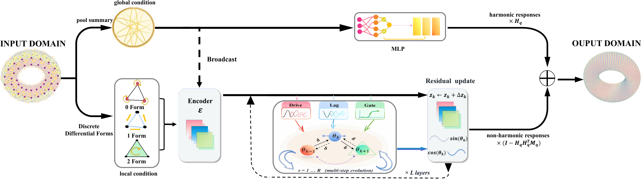
DKHO learns condition-dependent field interactions while preserving the domain’s differential structure. Its central design separates content states $z_{k}$ , which carry information for physical-field reconstruction, from relation states $\theta_{k}$ , which adapt cross-degree interactions through Kuramoto dynamics. The incidence operators fix the available interaction pathways, while the content states determine how the relation dynamics operates along them. As shown in Figure 2, DKHO first encodes conditions on native cochain supports (form-aware encoding), alternates relation evolution with content updates (conditional Dirac–Kuramoto coordination), and finally combines non-harmonic reconstruction with explicit topology-dependent harmonic response (Hodge-structured decoding).

4.1 Form-Aware Encoding

We encode each known PDE condition on its native geometric support. Vertex-sampled coefficients and Dirichlet data are assigned to vertices, line-integrated velocities or circulations to oriented edges, and areal sources or fluxes to faces. Each support also carries its geometric, orientation, and boundary descriptors. Writing $a_{k}$ for the degree- $k$ conditions and $g(a)$ for a pooled summary of the known inputs, we construct

F_{k}(a)=\operatorname{concat}\!\left(a_{k},\operatorname{Geo}_{k},\operatorname{Bnd}_{k},\operatorname{Pos}_{k},\operatorname{Broadcast}_{k}(g(a))\right)\in C^{k}\!\left(K;\mathbb{R}^{d_{k}^{\mathrm{in}}}\right).

(8)

This representation makes the support of each condition explicit before learned processing. Support-aware feature constructions are provided in Table 7 of Appendix B.5. Degree-specific encoders initialize the content states, while the relation states start from zero:

z_{k}^{(0)}=\operatorname{Enc}_{k}\!\left(F_{k}(a)\right)\in C^{k}\!\left(K;\mathbb{R}^{h}\right),\qquad\theta_{k}^{(0,0)}=0.

(9)

The content state $z_{k}$ represents information used to reconstruct the physical field. The real-valued relation state $\theta_{k}\in C^{k}(K;\mathbb{R}^{c\theta})$ instead provides a phase-inspired coordinate for adapting interactions along the fixed incidence structure.

4.2 Conditional Dirac–Kuramoto Coordination

The Dirac operator specifies the available pathways between adjacent degrees, but the same pathway can play different roles under different coefficients, forcing, or boundary conditions. DKHO adapts these interactions through relation dynamics inspired by simplicial Kuramoto models, in which phases on simplices interact through lower and upper incidence (Millán et al., 2020; Arnaudon et al., 2022; Nurisso et al., 2024). At layer $\ell$ , degree-specific maps of the content states produce a drive $\Omega_{k}^{(\ell)}$ , a signed gate $G_{k}^{(\ell)}\in(-1,1)$ , and a phase lag $\Lambda_{k}^{(\ell)}$ . These quantities control the intrinsic relation update, the contribution from an adjacent degree, and the offset in its interaction, respectively. A positive scalar $\sigma_{k}^{(\ell)}$ sets the feedback strength.

Interactions across degrees.

At each phase substep $r$ , we first compare each relation state with those on adjacent supports:

\displaystyle r_{k}^{\uparrow,(\ell,r)}=d_{k}\theta_{k}^{(\ell,r)}-G_{k+1}^{(\ell)}\odot\theta_{k+1}^{(\ell,r)},\quad r_{k}^{\downarrow,(\ell,r)}=\delta_{k}\theta_{k}^{(\ell,r)}+G_{k-1}^{(\ell)}\odot\theta_{k-1}^{(\ell,r)}.

(10)

The upper residual is defined on degree $k+1$ , and the lower residual on degree $k-1$ . Applying a sine nonlinearity and the corresponding return operator yields the degree- $k$ update:

\begin{split}\theta_{k}^{(\ell,r+1)}=\theta_{k}^{(\ell,r)}-\tau_{\ell}\Omega_{k}^{(\ell)}-\tau_{\ell}\sigma_{k}^{(\ell)}\delta_{k+1}\sin\!\left(r_{k}^{\uparrow,(\ell,r)}-\Lambda_{k+1}^{(\ell)}\right)\\ -\tau_{\ell}\sigma_{k}^{(\ell)}d_{k-1}\sin\!\left(r_{k}^{\downarrow,(\ell,r)}-\Lambda_{k-1}^{(\ell)}\right).\end{split}

(11)

Here $\tau_{\ell}$ is the update step size, and all degrees are updated synchronously using $\theta^{(\ell,r)}$ . The upper and lower feedback terms lie in $\operatorname{im}\delta_{k+1}$ and $\operatorname{im}d_{k-1}$ , respectively. Both therefore return to the correct support while retaining the distinction between coexact and exact interactions. Their contributions vary with the input through the learned gates, drives, and lags.

Connection to Hodge relaxation.

Setting the drive, gate, and lag to zero and the scale to one, the small-residual approximation $\sin(x)\simeq x$ gives

\theta_{k}^{(\ell,r+1)}-\theta_{k}^{(\ell,r)}\simeq-\tau_{\ell}\left(\delta_{k+1}d_{k}+d_{k-1}\delta_{k}\right)\theta_{k}^{(\ell,r)}=-\tau_{\ell}\Delta_{k}\theta_{k}^{(\ell,r)}.

(12)

Thus, the update recovers a discrete Hodge relaxation step in this limit. The learned dynamics extends this relaxation through nonlinear, condition-dependent interactions. These updates operate in latent computation. We present the derivation and parameterization details in Appendix B.3.

4.3 Phase-Modulated Hodge Decoding

Updating field content.

After $R$ relation substeps, a sine–cosine readout transfers the resulting coordination information to the content stream:

	$\displaystyle p_{k}^{(\ell)}$	$\displaystyle=W_{p,k}[\cos\theta_{k}^{(\ell,R)},\sin\theta_{k}^{(\ell,R)}]+b_{p,k},$		(13)
	$\displaystyle z_{k}^{(\ell+1)}$	$\displaystyle=\operatorname{Norm}_{k}\!\left(z_{k}^{(\ell)}+U_{k}[z_{k}^{(\ell)},p_{k}^{(\ell)}]+S_{k}z_{k}^{(0)}\right).$		(13)

The periodic readout modulates the content update, while the skip connection from $z_{k}^{(0)}$ retains access to the encoded conditions. Physical outputs are reconstructed from $z_{k}$ ; relation states are learned indirectly through the prediction objective and receive no separate supervision.

Separating non-harmonic and harmonic responses.

A pointwise decoder maps the final content at each requested degree $q$ to a provisional field $\widetilde{u}_{q}$ . Let $H_{q}$ contain an $M_{q}$ -orthonormal basis of the harmonic space $\mathcal{H}^{q}$ . We construct the prediction as

\widehat{u}_{q}=(I-H_{q}H_{q}^{\top}M_{q})\widetilde{u}_{q}+H_{q}T_{q}(g(a)),\qquad H_{q}^{\top}M_{q}H_{q}=I.

(14)

The first term projects the provisional field onto the non-harmonic subspace. The second predicts harmonic coordinates from the global input summary, providing an explicit path for topology-dependent responses. The two terms are orthogonal under $M_{q}$ , so the branches cannot duplicate the same harmonic component. When $\beta_{q}=0$ , the harmonic branch is omitted.

Together, the relation dynamics and Hodge decoder adapt differential interactions to each PDE instance while retaining a separate representation of global harmonic modes. Full architecture and optimization details are given in Appendix D.3.

5 Experiments

We evaluate DKHO on three PDE benchmarks with distinct geometric and topological structures: Darcy flow on a planar domain with two asymmetric holes, transport–diffusion on a closed torus embedded in three dimensions, and magnetostatics in a three-dimensional spherical shell. Each benchmark uses a fixed domain and probes a different aspect of field interaction: potential–flux coupling around obstacles, transport along noncontractible cycles, and the combination of local source-driven fields with global cavity responses.

5.1 Experimental Setup

Baselines.

We compare DKHO with six representative methods: GNO (Li et al., 2020) based on radius-graph kernel integration; FNO (Li et al., 2021) using truncated spectral convolutions; MGN (Pfaff et al., 2021) using iterative mesh message passing; DeepONet (Lu et al., 2021) using a branch–trunk representation; Geo-FNO (Li et al., 2023a) combining spectral propagation with geometric coordinate transformation; and HSD (Zheng et al., 2026) that separates harmonic and local responses through Hodge-aware representations.

Comparison protocol.

Each method is trained separately for each supervised output support, using common evaluation samples and target supports; training and selection protocols are detailed in Appendix D.2. The main tables evaluate baselines through their standard native input interfaces. For edge and face targets, methods without a rank-aware backbone use a fixed support-query decoder. HSD retains its rank-aware interface, while DKHO receives conditions on their native cochain supports.

To assess the effect of input information, we also report matched-condition comparisons in Appendix E.1. These augment baseline inputs with descriptors derived solely from known PDE conditions and fixed geometry, while retaining other settings unchanged. This control helps distinguish gains from richer input descriptors from those associated with DKHO’s structured computation.

Evaluation metrics.

Following Zheng et al. (2026), we compute all metrics after denormalization on the physical support of each supervised cochain, assessing three complementary aspects. Reconstruction accuracy is measured by MSE and mean relative $L^{2}$ error (RelL2); we emphasize RelL2 to facilitate comparisons across fields with different scales. Physical consistency is assessed through task-specific differential, energy, and spectral diagnostics. For a DEC operator $D_{k}\in{d_{k},\delta_{k}}$ , derivative fidelity measures the mean cosine agreement between $D_{k}\widehat{u}$ and $D_{k}u$ , rescaled to $[0,1]$ . Structural agreement is evaluated using $S_{\beta_{0}}$ , which compares connected-component counts of thresholded predictions and references across levels, and IoU, which measures overlap between high-response regions. Each main table reports an accuracy, a physical, and a structural metric.

For other implementation details, please refer to Appendix D.

5.2 Porous-Medium Darcy Flow

We consider anisotropic Darcy flow, $-\nabla\cdot(K\nabla p)=f$ , on a planar domain with two asymmetric holes (Bear, 1972; Boffi et al., 2013). Given source, coefficient, and boundary conditions, we predict vertex potentials $p_{0}\in C^{0}$ , oriented edge fluxes $q_{1}\in C^{1}$ , and face circulations $\omega_{2}=d_{1}q_{1}\in C^{2}$ , training each output separately. These targets assess reconstruction across the potential–flux–circulation chain on its native geometric supports. The domain has Betti numbers $(1,2,0)$ , with two independent noncontractible cycles around the holes.

As shown in Table 1, DKHO-large achieves the best performance across all three output supports and all reported metrics. Its RelL2 errors are $0.0035$ , $0.0155$ , and $0.0244$ for potential, flux, and circulation, respectively, reducing error by approximately 84%, 86%, and 78% relative to the best baseline on each target. These gains are accompanied by differential fidelities above 0.998 and improved structural agreement, indicating accurate reconstruction of both field values and their spatial variation. DKHO-small also outperforms every baseline across all reported metrics with only $64.1$ K parameters. These results demonstrate the effectiveness of DKHO across field supports, with particularly strong gains in flux and circulation prediction. Figure 3 provides a qualitative comparison.

Table 1: Darcy flow on a planar domain with two holes. Results are reported for vertex potentials (

C^{0}

), edge fluxes (

C^{1}

), and face circulations (

C^{2}

). Lower RelL2 and higher fidelity and structural scores indicate better performance. Bold and underline mark the best and second-best results.

Method Params (K) $C^{0}$ : potential $C^{1}$ : flux $C^{2}$ : circulation RelL2 $\downarrow$ Grad Fid $\uparrow$ $S_{\beta_{0}}$ $\uparrow$ RelL2 $\downarrow$ Co-diff Fid $\uparrow$ Curl Fid $\uparrow$ RelL2 $\downarrow$ Co-boundary Fid $\uparrow$ $S_{\beta_{0}}$ $\uparrow$ GNO 285.9 0.0326 0.9724 0.9589 0.1129 0.9915 0.9926 0.1104 0.9967 0.8775 FNO 216.4 0.1112 0.6838 0.8027 0.9736 0.6018 0.5066 0.9948 0.5460 0.3952 MGN 303.2 0.1176 0.8753 0.8526 0.2422 0.9842 0.9865 0.2420 0.9882 0.7201 DeepONet 559.1 0.0218 0.9696 0.9746 0.9459 0.6483 0.5133 0.9983 0.5171 0.3970 Geo-FNO 215.3 0.1536 0.9268 0.8626 0.9384 0.6430 0.5119 0.9581 0.6249 0.4099 HSD 200.4 0.0274 0.9360 0.9574 0.7624 0.7079 0.5169 0.9786 0.5837 0.4050 DKHO-small 64.1 0.0042 0.9985 0.9889 0.0264 0.9990 0.9986 0.0392 0.9996 0.9848 DKHO-large 243.1 0.0035 0.9989 0.9922 0.0155 0.9997 0.9996 0.0244 0.9998 0.9905

5.3 Torus Transport–Diffusion

We consider transport–diffusion on a closed torus in three dimensions (Dziuk and Elliott, 2013):

\partial_{t}u+\nabla_{\mathcal{M}}\cdot(uv)=\kappa\Delta_{\mathcal{M}}u,

(15)

where $v$ is a prescribed tangent velocity and $\kappa$ is the diffusion coefficient. Given the initial scalar field and velocity, we predict terminal concentration $u^{T}\in C^{0}$ , oriented edge transport $q^{T}\in C^{1}$ , and face-integrated mass $m^{T}\in C^{2}$ , training each output separately. The torus has Betti numbers $(1,2,1)$ , allowing transport around two independent noncontractible cycles. This benchmark therefore tests reconstruction of local advective and diffusive behavior alongside global recirculation.

Table 2 shows that DKHO-large achieves the best performance across all three output supports and all reported metrics. Its RelL2 errors of $0.1413$ , $0.1262$ , and $0.1007$ for concentration, flux, and mass correspond to reductions of approximately 42%, 20%, and 12% relative to the best baseline on each target. Notably, flux Curl Fid improves from MGN’s $0.7160$ to 0.8187, highlighting a substantial gain in reconstructing the differential structure of transport. DKHO-small also remains competitive with only $63.5$ K parameters. These results support accurate and parameter-efficient transport prediction across multiple field supports. Figure 4 provides a qualitative comparison.

Table 2: Transport–diffusion on a closed torus. Results are reported for terminal concentration (

C^{0}

), oriented edge transport (

C^{1}

), and face-integrated mass (

C^{2}

). Lower RelL2 and higher physical and structural scores indicate better performance.

Method Params (K) Concentration $C^{0}$ Flux $C^{1}$ Mass $C^{2}$ RelL2 $\downarrow$ Grad Fid $\uparrow$ $S_{\beta_{0}}$ $\uparrow$ RelL2 $\downarrow$ Curl Fid $\uparrow$ Energy Fid $\uparrow$ RelL2 $\downarrow$ Co-boundary Fid $\uparrow$ $S_{\beta_{0}}$ $\uparrow$ GNO 285.9 0.4093 0.6537 0.4891 0.3753 0.5605 0.8660 0.2154 0.8877 0.6500 FNO 262.8 0.2440 0.7353 0.6571 0.6687 0.5116 0.6243 0.4175 0.6176 0.3892 MGN 303.2 0.2849 0.7406 0.6708 0.1581 0.7160 0.9721 0.1139 0.9567 0.7102 DeepONet 273.2 0.4578 0.5550 0.4199 0.6891 0.5094 0.6007 0.4631 0.6483 0.2996 Geo-FNO 220.0 0.3681 0.6693 0.4782 0.7077 0.5085 0.5816 0.4879 0.6456 0.3037 HSD 241.0 0.3613 0.7600 0.5976 0.3673 0.5542 0.8623 0.3699 0.6430 0.4431 DKHO-small 63.5 0.1428 0.8440 0.8083 0.1310 0.8026 0.9750 0.1142 0.9666 0.7518 DKHO-large 242.3 0.1413 0.8472 0.8133 0.1262 0.8187 0.9758 0.1007 0.9737 0.7736

5.4 Cavity Magnetostatic Response

We finally study a magnetostatic response governed by $\nabla\times H=0$ , $\nabla\cdot B=0$ , and $B=H+M$ (Jackson, 1999; Bossavit, 1998) on the spherical shell $\Omega=B(0,2.0)\setminus\overline{B}(0,0.4)$ . The learning task maps nodal source conditions to a flux-like $2$ -form response, evaluated through a three-channel nodal-vector readout. This benchmark combines local source-driven fields with a global cavity-scale response, testing whether an operator can reconstruct both within the same domain.

As shown in Table 3, DKHO-large achieves the best performance across all reported prediction metrics. Its RelL2 of $0.0140$ represents an approximately 74% reduction over HSD’s $0.0547$ . The improvement is particularly pronounced in Curl MSE, which decreases from $7.03\times 10^{-3}$ to $\mathbf{3.92\times 10^{-4}}$ , a reduction of approximately 94%. IoU also increases from $0.8268$ to $0.9724$ , indicating closer agreement in high-response regions. DKHO-small surpasses all baselines with only $64.5$ K parameters. These results demonstrate gains in field reconstruction, differential fidelity, and spatial structure. Figure 5 visualizes the predicted response and local errors around the cavity.

Table 3: Magnetostatic response on a spherical shell. The flux-like

2

-form response is evaluated through a three-channel nodal-vector readout. Lower errors and higher fidelity and IoU scores indicate better performance. Bold and underline mark the best and second-best values.

Method	Params (K)	MSE $\downarrow$	RelL2 $\downarrow$	Div Fid $\uparrow$	Curl MSE $\downarrow$	Vort Fid $\uparrow$	Enst Fid $\uparrow$	Energy Fid $\uparrow$	IoU $\uparrow$
GNO	231.5	2.30e-3	1.1030	0.5673	1.5409	0.4970	0.2387	0.3714	0.1400
FNO	227.4	4.59e-5	0.1189	0.9887	1.93e-2	0.9098	0.8721	0.9053	0.7242
MGN	246.6	1.66e-4	0.2532	0.9590	6.10e-2	0.8008	0.6970	0.8752	0.5555
DeepONet	238.9	1.07e-5	0.0814	0.9967	1.07e-2	0.9361	0.8356	0.9661	0.7984
Geo-FNO	252.7	4.23e-5	0.1152	0.9895	1.61e-2	0.9236	0.8870	0.9091	0.7234
HSD	265.4	7.20e-6	0.0547	0.9981	7.03e-3	0.9675	0.9513	0.9681	0.8268
DKHO-small	64.5	1.30e-6	0.0179	0.9996	5.36e-4	0.9975	0.9875	0.9914	0.9650
DKHO-large	243.5	9.11e-7	0.0140	0.9997	3.92e-4	0.9983	0.9913	0.9940	0.9724

5.5 Ablations and Further Analyses

We conduct controlled ablations and further analyses to examine the roles of DKHO’s components. Ablations of DKHO-small reveal complementary contributions from Dirac routing, relation dynamics, and harmonic decoding. Removing routing causes the largest accuracy losses on Darcy and torus targets, raising Darcy $C^{2}$ error to nearly $\bf{12}\bm{\times}$ that of the full model. Removing the relation state degrades all seven targets, most notably cavity magnetostatics, while harmonic decoding improves every applicable target. Full ablations and parameter-efficiency comparisons appear in Appendix E.2 (Table 21). Frozen-model analyses further show above-chance spatial overlap between learned phase updates and physical field structures (Appendix E.3).

6 Conclusion

We introduced DKHO, a neural operator that combines explicit geometric and topological structure with condition-dependent field interactions. Form-aware encoding retains the native supports of PDE conditions, Kuramoto-inspired dynamics adapts coordination along fixed Dirac pathways, and Hodge-structured decoding separates non-harmonic and harmonic responses. Across Darcy flow, torus transport–diffusion, and cavity magnetostatics, DKHO improves prediction accuracy and differential and structural fidelity, while its compact variant remains competitive with substantially fewer parameters. Ablations further support the complementary contributions of structured routing, relation dynamics, and harmonic decoding. These findings highlight adaptive coordination within prescribed differential structure as a useful inductive bias for PDE operator learning. Extending DKHO beyond fixed domains to varying geometries and topologies is an important future direction.

7 AI USE STATEMENT

In this work, we used generative AI tools for limited assistance with code development and language editing. Their use was restricted to improving code implementation and the clarity, grammar, and readability of the manuscript; they were not used to generate, alter, or determine the reported experimental results. The authors retain full responsibility for the accuracy, validity, and integrity of the final manuscript, including its text, claims, experimental results, and accompanying artifacts.

References

Arnaudon et al. (2022) A. Arnaudon, R. L. Peach, G. Petri, and P. Expert Connecting Hodge and Sakaguchi–Kuramoto through a mathematical framework for coupled oscillators on simplicial complexes. Communications Physics 5 (1), pp. 211. External Links: Document Cited by: §B.3, §B.3, §1, §2, §4.2.
Arnold et al. (2006) D. N. Arnold, R. S. Falk, and R. Winther Finite element exterior calculus, homological techniques, and applications. Acta Numerica 15, pp. 1–155. External Links: Document Cited by: Appendix A, §1, §2.
Badolia et al. (2026) P. Badolia, L. Obukhov, D. Bylinkin, and A. Beznosikov The Kuramoto neural operator: learning to solve PDEs via coupled oscillator dynamics. arXiv preprint arXiv:2608.10234. External Links: Link Cited by: §2.
Bastian et al. (2026) L. Bastian, S. Leventhal, M. Hajij, and T. Birdal Topological neural operators. arXiv preprint arXiv:2606.09806. External Links: Link Cited by: §B.1, §1, §2.
Bear (1972) J. Bear Dynamics of fluids in porous media. American Elsevier, New York, NY, USA. Cited by: §5.2.
Bodnar et al. (2021) C. Bodnar, F. Frasca, Y. Wang, N. Otter, G. F. Montúfar, P. Liò, and M. Bronstein Weisfeiler and Lehman go topological: message passing simplicial networks. In Proceedings of the 38th International Conference on Machine Learning, Proceedings of Machine Learning Research, Vol. 139, pp. 1026–1037. External Links: Link Cited by: §2.
Boffi et al. (2013) D. Boffi, F. Brezzi, and M. Fortin Mixed finite element methods and applications. Springer Series in Computational Mathematics, Vol. 44, Springer, Berlin, Heidelberg, Germany. External Links: Document Cited by: §5.2.
Bossavit (1998) A. Bossavit Computational electromagnetism: variational formulations, complementarity, edge elements. Academic Press, San Diego, CA, USA. Cited by: §5.4.
Dai and Song (2026) J. Dai and Y. Song Winfree oscillatory neural network. arXiv preprint arXiv:2605.20922. External Links: Link Cited by: §2.
Desbrun et al. (2005) M. Desbrun, A. N. Hirani, M. Leok, and J. E. Marsden Discrete exterior calculus. arXiv preprint arXiv:math/0508341. External Links: Link Cited by: Appendix A, §1, §2.
Dziuk and Elliott (2013) G. Dziuk and C. M. Elliott Finite element methods for surface PDEs. Acta Numerica 22, pp. 289–396. External Links: Document Cited by: §5.3.
Ebli et al. (2020) S. Ebli, M. Defferrard, and G. Spreemann Simplicial neural networks. arXiv preprint arXiv:2010.03633. Note: NeurIPS 2020 Workshop on Topological Data Analysis and Beyond External Links: Link Cited by: §2.
Hajij et al. (2022) M. Hajij, G. Zamzmi, T. Papamarkou, N. Miolane, A. Guzmán-Sáenz, K. Natesan Ramamurthy, T. Birdal, T. K. Dey, S. Mukherjee, S. N. Samaga, N. Livesay, R. Walters, P. Rosen, and M. T. Schaub Topological deep learning: going beyond graph data. arXiv preprint arXiv:2206.00606. External Links: Link Cited by: §2.
Hirani (2003) A. N. Hirani Discrete exterior calculus. Ph.D. Thesis, California Institute of Technology, Pasadena, CA, USA. Cited by: Appendix A, §1, §2.
Jackson (1999) J. D. Jackson Classical electrodynamics. 3 edition, Wiley, New York, NY, USA. Cited by: §5.4.
Kovachki et al. (2023) N. Kovachki, Z. Li, B. Liu, K. Azizzadenesheli, K. Bhattacharya, A. Stuart, and A. Anandkumar Neural operator: learning maps between function spaces with applications to PDEs. Journal of Machine Learning Research 24 (89), pp. 1–97. External Links: Link Cited by: §1, §2.
Li et al. (2023a) Z. Li, D. Z. Huang, B. Liu, and A. Anandkumar Fourier neural operator with learned deformations for PDEs on general geometries. Journal of Machine Learning Research 24 (388), pp. 1–26. External Links: Link Cited by: §1, §2, §5.1.
Li et al. (2020) Z. Li, N. Kovachki, K. Azizzadenesheli, B. Liu, K. Bhattacharya, A. Stuart, and A. Anandkumar Neural operator: graph kernel network for partial differential equations. arXiv preprint arXiv:2003.03485. External Links: Link Cited by: §2, §5.1.
Li et al. (2021) Z. Li, N. Kovachki, K. Azizzadenesheli, B. Liu, K. Bhattacharya, A. Stuart, and A. Anandkumar Fourier neural operator for parametric partial differential equations. In International Conference on Learning Representations, External Links: Link Cited by: §1, §2, §5.1.
Li et al. (2023b) Z. Li, N. B. Kovachki, C. Choy, B. Li, J. Kossaifi, S. P. Otta, M. A. Nabian, M. Stadler, C. Hundt, K. Azizzadenesheli, and A. Anandkumar Geometry-informed neural operator for large-scale 3D PDEs. In Advances in Neural Information Processing Systems, Vol. 36, pp. 35836–35854. External Links: Link Cited by: §1, §2.
Liu et al. (2023) N. Liu, S. Jafarzadeh, and Y. Yu Domain agnostic Fourier neural operators. In Advances in Neural Information Processing Systems, Vol. 36, pp. 47438–47450. External Links: Link Cited by: §2.
Lu et al. (2021) L. Lu, P. Jin, G. Pang, Z. Zhang, and G. E. Karniadakis Learning nonlinear operators via DeepONet based on the universal approximation theorem of operators. Nature Machine Intelligence 3 (3), pp. 218–229. External Links: Document Cited by: §1, §2, §5.1.
Millán et al. (2020) A. P. Millán, J. J. Torres, and G. Bianconi Explosive higher-order Kuramoto dynamics on simplicial complexes. Physical Review Letters 124 (21), pp. 218301. External Links: Document Cited by: §2, §4.2.
Miyato et al. (2025) T. Miyato, S. Löwe, A. Geiger, and M. Welling Artificial Kuramoto oscillatory neurons. In International Conference on Learning Representations, External Links: Link Cited by: §2.
Nurisso et al. (2024) M. Nurisso, A. Arnaudon, M. Lucas, R. L. Peach, P. Expert, F. Vaccarino, and G. Petri A unified framework for simplicial Kuramoto models. Chaos: An Interdisciplinary Journal of Nonlinear Science 34 (5), pp. 053118. External Links: Document Cited by: §B.3, §B.3, §B.3, §B.3, §B.3, §B.3, §1, §2, §4.2.
Pfaff et al. (2021) T. Pfaff, M. Fortunato, A. Sanchez-Gonzalez, and P. W. Battaglia Learning mesh-based simulation with graph networks. In International Conference on Learning Representations, External Links: Link Cited by: §2, §5.1.
Song et al. (2025) Y. Song, T. A. Keller, S. Brodjian, T. Miyato, Y. Yue, P. Perona, and M. Welling Kuramoto orientation diffusion models. In Advances in Neural Information Processing Systems, Vol. 38. External Links: Link Cited by: §2.
Wu et al. (2024) H. Wu, H. Luo, H. Wang, J. Wang, and M. Long Transolver: a fast transformer solver for PDEs on general geometries. In Proceedings of the 41st International Conference on Machine Learning, Proceedings of Machine Learning Research, Vol. 235, pp. 53681–53705. External Links: Link Cited by: §1, §2.
Zheng et al. (2026) D. Zheng, T. Zhong, and C. Allen-Blanchette Topology-preserving neural operator learning via Hodge decomposition. In Proceedings of the 43rd International Conference on Machine Learning, External Links: Link Cited by: §1, §2, §5.1, §5.1.

Appendix

Appendix A Notation and Algebraic-Topological Primer

This section develops the cochain and Hodge structure used in Section 3. We distinguish incidence, which records connectivity and orientation, from the metric, which determines inner products and adjoint operators. The definitions follow discrete exterior calculus (DEC) and finite-element exterior calculus (Hirani, 2003; Desbrun et al., 2005; Arnold et al., 2006); Table 4 summarizes the notation.

Table 4: Notation for discrete fields and DKHO. The degree

k

specifies a geometric support; channel dimensions specify the quantities carried on that support.

Geometry and cochains
Symbol	Definition
$(\mathcal{M},g)$ , $K$	Oriented Riemannian domain and its oriented simplicial discretization.
$K_{k}$ , $N_{k}$	Set of oriented $k$ -simplices and its cardinality.
$\Omega^{k}(\mathcal{M})$ , $C^{k}(K;\mathbb{R}^{c})$	Smooth $k$ -forms and discrete $k$ -cochains with $c$ channels.
$u_{k}$ , $a$	Physical output cochain and known PDE conditions.
Differential operators and topology
$B_{k}\in\mathbb{R}^{N_{k-1}\times N_{k}}$	Signed boundary-incidence matrix.
$d_{k}=B_{k+1}^{\top}$	Coboundary: $C^{k}\to C^{k+1}$ .
$M_{k}\in\mathbb{R}^{N_{k}\times N_{k}}$	Positive definite Hodge mass matrix.
$\delta_{k}=M_{k-1}^{-1}d_{k-1}^{\top}M_{k}$	Metric-adjoint derivative: $C^{k}\to C^{k-1}$ .
$\mathcal{D}=d+\delta$ , $\Delta_{k}$	Graded Dirac operator and degree- $k$ Hodge Laplacian.
$\mathcal{H}^{k}$ , $\beta_{k}$	Harmonic space $\ker\Delta_{k}$ and its dimension.
$H_{k}$ , $\Pi_{k}^{\mathcal{H}}$	$M_{k}$ -orthonormal harmonic basis and orthogonal projector.
Learned states and dynamics
$z_{k}\in\mathbb{R}^{N_{k}\times h}$	Content state carrying the field representation.
$\theta_{k}\in\mathbb{R}^{N_{k}\times c_{\theta}}$	Real-valued, phase-inspired relation state.
$r_{k}^{\uparrow}$ , $r_{k}^{\downarrow}$	Relation residuals on degrees $k+1$ and $k-1$ .
$\Omega_{k}$ , $G_{k}$ , $\Lambda_{k}$ , $\sigma_{k}$	Content-dependent drive, gate, and lag; positive feedback scale.
$L$ , $R$ , $\tau_{\ell}$	Number of layers, phase substeps, and layer-wise step size.

A.1 Physical forms and discrete cochains

Geometric support.

Let $K$ be a finite oriented simplicial complex approximating an $n$ -dimensional domain $\mathcal{M}$ . Its simplices are closed under taking faces, and two simplices intersect in a common face or not at all. Fix one orientation for each simplex. The chain space $C_{k}(K)$ consists of real linear combinations of these oriented simplices; its dual is the cochain space

C^{k}(K;\mathbb{R}^{c})=\operatorname{Hom}(C_{k}(K),\mathbb{R}^{c})\cong\mathbb{R}^{N_{k}\times c}.

(16)

A cochain assigns a value to each oriented simplex, with $u_{k}(-\sigma)=-u_{k}(\sigma)$ . The degree determines where the value is measured, independently of the number of channels.

From a physical field to a cochain.

The de Rham map discretizes a smooth form by integration,

(I_{k}\omega)(\sigma)=\int_{\sigma}\omega,\qquad I_{k}:\Omega^{k}(\mathcal{M})\to C^{k}(K).

(17)

For $k=0$ , this is point evaluation. In an oriented three-dimensional domain, representative measurements are

p_{0}(v)=p(v),\qquad q_{1}(e)=\int_{e}\mathbf{q}\cdot\mathbf{t}\,ds,\qquad b_{2}(f)=\int_{f}\mathbf{B}\cdot\mathbf{n}\,dS.

(18)

Here $\mathbf{t}$ and $\mathbf{n}$ follow the edge and face orientations. On a two-dimensional surface, an areal density instead gives the top-degree cochain $m_{2}(f)=\int_{f}u\,dA$ . Thus an edge integral and a surface flux can originate from vector fields yet have different degrees: the measurement, rather than the array’s channel count, determines the form type.

A.2 Boundary and discrete exterior derivative

Signed incidence.

For an oriented $k$ -simplex, the boundary is

\partial_{k}[v_{0},\ldots,v_{k}]=\sum_{j=0}^{k}(-1)^{j}[v_{0},\ldots,\widehat{v}_{j},\ldots,v_{k}],\qquad B_{k}\in\mathbb{R}^{N_{k-1}\times N_{k}}.

(19)

The hat denotes an omitted vertex. An entry of $B_{k}$ is $+1$ or $-1$ when the corresponding face occurs with the same or opposite orientation, and zero otherwise. The coboundary is its dual:

d_{k}=B_{k+1}^{\top}:C^{k}(K)\to C^{k+1}(K),\qquad(d_{k}u)(\sigma)=u(\partial_{k+1}\sigma).

(20)

This is the discrete Stokes identity: a derivative measured on a simplex equals the oriented sum over its boundary.

Edge and face examples.

For $e=[v_{i},v_{j}]$ and $f=[v_{i},v_{j},v_{\ell}]$ ,

(d_{0}p)(e)=p_{j}-p_{i},\qquad(d_{1}q)(f)=q_{j\ell}-q_{i\ell}+q_{ij}.

(21)

The first is a potential difference; the second is the circulation around a triangle. Substituting $q=d_{0}p$ into the second expression cancels all vertex values. More generally, $\partial_{k}\partial_{k+1}=0$ gives

C^{k-1}(K)\xrightarrow{\,d_{k-1}\,}C^{k}(K)\xrightarrow{\,d_{k}\,}C^{k+1}(K),\qquad d_{k}d_{k-1}=0.

(22)

For exact integration of smooth forms, Stokes’ theorem also yields

I_{k+1}(d\omega)=d_{k}(I_{k}\omega).

(23)

These identities explain why incidence operators provide compatible paths between field supports. Their algebraic cancellation remains exact on the complex; nonlinear maps inserted between derivatives need not preserve the same cancellation.

A.3 Metric adjoints and Hodge decomposition

Metric and adjoint.

A symmetric positive definite mass matrix $M_{k}$ defines

\langle u,v\rangle_{M_{k}}=u^{\top}M_{k}v,\qquad\|u\|_{M_{k}}^{2}=u^{\top}M_{k}u.

(24)

It represents the discrete Hodge inner product, approximating $\int_{\mathcal{M}}\omega\wedge\star\eta$ . For multichannel cochains, the pairing is summed over channels. The codifferential is determined by $\langle d_{k-1}a,b\rangle_{M_{k}}=\langle a,\delta_{k}b\rangle_{M_{k-1}}$ , hence

\delta_{k}=M_{k-1}^{-1}d_{k-1}^{\top}M_{k},\qquad\Delta_{k}=\underbrace{d_{k-1}\delta_{k}}_{\text{lower-degree term}}+\underbrace{\delta_{k+1}d_{k}}_{\text{upper-degree term}}.

(25)

Out-of-range maps vanish at degrees zero and $n$ . Unlike incidence, $\delta_{k}$ and $\Delta_{k}$ depend on the metric. The matrix $\Delta_{k}$ is self-adjoint in the $M_{k}$ inner product, with

\langle u,\Delta_{k}u\rangle_{M_{k}}=\|\delta_{k}u\|_{M_{k-1}}^{2}+\|d_{k}u\|_{M_{k+1}}^{2}\geq 0.

(26)

Consequently, $\ker\Delta_{k}=\ker d_{k}\cap\ker\delta_{k}$ . With $M_{0}=M_{1}=I$ , $\Delta_{0}=B_{1}B_{1}^{\top}$ is the usual vertex graph Laplacian. For general $M_{k}$ , the Euclidean-symmetric representation is $M_{k}^{1/2}\Delta_{k}M_{k}^{-1/2}$ .

Orthogonal field components.

The finite-dimensional Hodge decomposition is

C^{k}(K)=\operatorname{im}d_{k-1}\oplus_{M_{k}}\mathcal{H}^{k}\oplus_{M_{k}}\operatorname{im}\delta_{k+1},\qquad\mathcal{H}^{k}=\ker\Delta_{k}.

(27)

The three components are exact, harmonic, and coexact. Exact fields satisfy $d_{k}u_{k}^{\rm ex}=0$ ; coexact fields satisfy $\delta_{k}u_{k}^{\rm coex}=0$ ; harmonic fields satisfy both. Their orthogonality follows from adjointness and $d_{k}d_{k-1}=0$ . In particular,

	$\displaystyle u_{k}$	$\displaystyle=\underbrace{d_{k-1}a_{k-1}}_{u_{k}^{\rm ex}}+\underbrace{h_{k}}_{u_{k}^{\mathcal{H}}}+\underbrace{\delta_{k+1}b_{k+1}}_{u_{k}^{\rm coex}},$		(28)
	$\displaystyle\\|u_{k}\\|_{M_{k}}^{2}$	$\displaystyle=\\|u_{k}^{\rm ex}\\|_{M_{k}}^{2}+\\|u_{k}^{\mathcal{H}}\\|_{M_{k}}^{2}+\\|u_{k}^{\rm coex}\\|_{M_{k}}^{2}.$		(28)

The components are unique, although the potentials $a_{k-1}$ and $b_{k+1}$ may have gauge freedom. For edge fields, exact and coexact components generalize gradient-type and circulation-type responses; at other degrees, the operator ranges give the precise interpretation.

Graded interactions.

The Dirac operator combines adjacent-degree maps: $(\mathcal{D}v)_{k}=d_{k-1}v_{k-1}+\delta_{k+1}v_{k+1}$ . Since $d^{2}=\delta^{2}=0$ , its square acts degree-wise as $(\mathcal{D}^{2}v)_{k}=\Delta_{k}v_{k}$ . This is the connection between the routing in Eq. (5) and the Hodge relaxation limit derived in Appendix B.3.

A.4 Cohomology, harmonic modes, and boundary conditions

Topology and harmonic dimension.

The quotient of closed cochains by exact cochains defines cohomology:

H^{k}(K;\mathbb{R})=\ker d_{k}/\operatorname{im}d_{k-1},\qquad\beta_{k}=\dim H^{k}(K;\mathbb{R})=\dim\mathcal{H}^{k}.

(29)

Every cohomology class has a unique harmonic representative for a fixed inner product. Topology determines the dimension, whereas the metric determines the representative and its spatial profile. For a closed $k$ -cycle $c_{k}$ and an exact cochain,

(d_{k-1}a)(c_{k})=a(\partial_{k}c_{k})=0.

(30)

A nonzero period of a closed cochain around such a cycle therefore detects a component that cannot be expressed as an exact field.

For the full complexes used to describe the benchmark geometries, $(\beta_{0},\beta_{1},\beta_{2})$ equals $(1,2,0)$ for the perforated Darcy domain, $(1,2,1)$ for the torus, and $(1,0,1)$ for the spherical shell. These numbers describe connected components, independent one-cycles, and independent two-cycles. For the torus, $\beta_{2}=1$ corresponds to its closed surface; for the shell, it corresponds to a surface enclosing the cavity.

Boundary conditions and harmonic readout.

Boundary restrictions must be specified before interpreting a Laplacian null space. The full cochain complex yields ordinary cohomology; the relative complex $C^{\bullet}(K,\partial K)$ instead yields relative cohomology. Imposing a boundary condition can therefore change the relevant harmonic dimension. The Betti numbers above describe the unrestricted domain topology, rather than the nullity of every boundary-conditioned PDE matrix.

For a chosen complex and metric, an $M_{k}$ -orthonormal harmonic basis $H_{k}\in\mathbb{R}^{N_{k}\times\beta_{k}}$ gives

H_{k}^{\top}M_{k}H_{k}=I,\qquad\Pi_{k}^{\mathcal{H}}=H_{k}H_{k}^{\top}M_{k},\qquad u_{k}^{\mathcal{H}}=H_{k}(H_{k}^{\top}M_{k}u_{k}).

(31)

This finite-dimensional representation motivates DKHO’s harmonic readout in Eq. (14). A nonzero $\beta_{k}$ permits a harmonic response; its coefficient is set by the PDE conditions and need not vary across samples.

A.5 Form-valued PDE representations

Field type and balance laws.

The same calculus describes physical systems through the supports of their observables. A vector field $\mathbf{v}$ on a Riemannian domain defines the line-integral form $\mathbf{v}^{\flat}=g(\mathbf{v},\cdot)$ and the flux form $\star\mathbf{v}^{\flat}$ of degree $n-1$ . In three dimensions these have degrees one and two, respectively. With the adjoint convention used above, $\delta\mathbf{v}^{\flat}=-\nabla\cdot\mathbf{v}$ in the interior, and $\Delta_{0}=\delta d=-\Delta_{\rm LB}$ . These signs distinguish the positive Hodge Laplacian from the usual diffusion generator.

Table 5 gives representative continuum systems; compatible discretization replaces their derivatives by the matrices above. The table specifies constitutive and balance relations, while boundary data and material assumptions complete each problem. Appendix B.2 specializes this representation to our three benchmarks.

Table 5: Representative PDEs in differential-form notation.

d

and

\delta

denote continuum derivatives here;

\delta=d^{*}

and

\Delta_{0}=\delta d

. Material coefficients are written in their simplest scalar form. The fields and operators are discretized on matching supports.

System	Physical forms	Governing relations
Darcy flow	Potential $p\in\Omega^{0}$ ; line flux $q\in\Omega^{1}$	$q=-\kappa\,dp$ , $-\delta q=f$
Heat diffusion	Temperature $u\in\Omega^{0}$ ; heat flux $q\in\Omega^{1}$	$q=-\kappa\,du$ , $\partial_{t}u-\delta q=s$
Surface transport	Density $u\in\Omega^{0}$ ; transport $j\in\Omega^{1}$	$j=uv^{\flat}-\kappa\,du$ , $\partial_{t}u-\delta j=0$
Magnetostatics (3D)	Field $H\in\Omega^{1}$ ; flux $B\in\Omega^{2}$	$dB=0$ , $dH=J$ , $B=\mu\star H$
Maxwell system (3D)	$E,H\in\Omega^{1}$ ; $D,B,J\in\Omega^{2}$	$\partial_{t}B+dE=0$ , $\partial_{t}D-dH=-J$
Reaction–diffusion	Species $u\in\Omega^{0}$ ; diffusive flux $q\in\Omega^{1}$	$q=-\kappa\,du$ , $\partial_{t}u-\delta q=R(u)$

Benchmark observables.

Darcy evaluates the potential $p_{0}$ , oriented line flux $q_{1}$ , and derived face circulation $d_{1}q_{1}$ . Torus transport evaluates terminal concentration, edge transport, and face-integrated mass; the last is an area measurement of the scalar density, not an exterior derivative of the edge transport. The cavity response is interpreted through magnetic surface flux but evaluated with a three-channel nodal-vector readout. This distinction between physical form degree and numerical readout keeps the field interpretation separate from its storage convention.

Appendix B Mathematical Foundations of Form-Valued PDE Operators

Appendix A establishes the cochain spaces and discrete operators. Here we use them to connect physical observables, conditional relation dynamics, and field reconstruction. The derivation separates the established simplicial Kuramoto model from the learned cross-degree interactions introduced in Section 4.2.

B.1 A form-valued operator-learning problem

Conditions and unknowns.

On a fixed oriented complex $K$ , let $a$ collect the known material coefficients, sources, boundary data, and, for evolution problems, initial conditions. Following the typed formulation of Bastian et al. (2026), a single-degree discrete PDE has the form

\mathcal{F}_{k}\!\left(u_{k},d_{k}u_{k},\delta_{k}u_{k},\Delta_{k}u_{k};a\right)=0,\qquad u_{k}\in C^{k}(K;\mathbb{R}^{c_{k}}),

(32)

where $\mathcal{F}_{k}$ returns a residual on degree $k$ ; its arguments retain their respective supports. Coupled systems instead act on a graded field $u=(u_{0},\ldots,u_{d})$ :

\mathcal{F}_{k}\!\left(\{u_{j}\},\{d_{j}u_{j}\},\{\delta_{j}u_{j}\},\{\Delta_{j}u_{j}\};a\right)=0,\qquad k=0,\ldots,d.

(33)

For time-dependent problems, $\mathcal{F}_{k}$ also takes $\partial_{t}u_{k}$ as an argument. Boundary conditions and any gauge constraints complete the problem. The elementary degree-changing routes are $d_{k-1}u_{k-1}\in C^{k}$ and $\delta_{k+1}u_{k+1}\in C^{k}$ ; constitutive maps specify how these quantities enter a particular PDE.

Solution maps and observation maps.

For admissible conditions that determine a unique solution, the learning target can be written as

\mathcal{G}_{K}:\mathcal{A}(K)\longrightarrow\mathcal{Y}(K),\qquad a\longmapsto\mathcal{R}_{K}u^{\star}(a),\qquad\mathcal{Y}(K)=\bigoplus_{q\in\mathcal{Q}}C^{q}(K;\mathbb{R}^{r_{q}}),

(34)

where $\mathcal{A}(K)$ contains the input cochains and global parameters, $\mathcal{Q}$ indexes the requested output supports, and $\mathcal{R}_{K}$ specifies sampling or integration of the solution. For transport, $u^{\star}(a)$ is evaluated at the prescribed terminal time. This separates the physical solution from its numerical observation: several supervised cochains may be derived from one underlying field. DKHO approximates this map by learning condition-dependent interactions on fixed differential routes; its latent iteration index is independent of physical time. The cochain formulation provides the structural prior, while approximation accuracy is assessed by the experiments.

B.2 Benchmark instantiations and DEC realization

The three benchmarks instantiate different observation maps in Eq. (34). We use the sign convention of Appendix A.5: $\delta\mathbf{v}^{\flat}=-\nabla\!\cdot\mathbf{v}$ and $\Delta_{0}=\delta d\geq 0$ .

Darcy: potential, line flux, and circulation.

On the perforated planar domain, let $p$ be the scalar potential and $q=\mathbf{q}^{\flat}$ the one-form associated with the Darcy velocity. For a positive constitutive operator $\mathcal{K}$ on one-forms,

q=-\mathcal{K}\,dp,\qquad-\delta q=f,\qquad\delta(\mathcal{K}\,dp)=f.

(35)

The corresponding discrete relations are $q_{1}=-\mathcal{K}_{1}d_{0}p_{0}$ and $-\delta_{1}q_{1}=f_{0}$ , with boundary traces imposed separately. Here $\mathcal{K}_{1}:C^{1}\to C^{1}$ includes the discretized anisotropic coefficient. The observables are $p_{0}$ , $q_{1}$ , and $\omega_{2}=d_{1}q_{1}$ . Although $d_{1}d_{0}=0$ , generally $d_{1}\mathcal{K}_{1}d_{0}\neq 0$ : spatially varying or anisotropic constitutive response can produce nonzero flux circulation. Thus $C^{2}$ evaluates structure beyond the potential difference itself.

Toroidal transport: concentration, transport, and mass.

On the closed torus with tangent velocity $v$ and constant diffusivity $\kappa$ , the transport one-form is $j=uv^{\flat}-\kappa\,du$ . Conservation gives

\partial_{t}u-\delta j=0,\qquad\partial_{t}u-\delta(uv^{\flat})=-\kappa\Delta_{0}u,

(36)

which implies conservation of $\int u\,dA$ on a closed surface. At terminal time, the benchmark records vertex concentration, oriented edge transport, and face mass. The last is the two-cochain $m_{f}=\int_{f}u(T)\,dA$ , approximated by face quadrature; it is an integrated density, whereas $d_{1}j_{1}$ is a circulation. This distinction explains why equal cochain degrees need not imply equal physical observables.

Cavity magnetostatics: a flux form with a vector readout.

In three dimensions, magnetic induction is the two-form $\mathcal{B}=\star\mathbf{B}^{\flat}$ , while the magnetic field is the one-form $\mathcal{H}=\mathbf{H}^{\flat}$ . For the current-free, nondimensional magnetization setting described in the main text,

d\mathcal{B}=0,\qquad d\mathcal{H}=0,\qquad\mathcal{B}=\star(\mathcal{H}+\mathbf{M}^{\flat}).

(37)

The surface measurement is $b_{f}=\int_{f}\mathcal{B}=\int_{f}\mathbf{B}\cdot\mathbf{n}_{f}\,dA$ . The benchmark instead stores the flux-like response as three vector components per node for prediction and evaluation. This array belongs to $C^{0}(K;\mathbb{R}^{3})$ as stored; the associated physical flux observable has degree two. The two descriptions are connected by reconstruction and surface integration, not by identifying three channels with a cochain degree. These continuum relations supply the physical interpretation; dataset construction and numerical readouts are specified in Appendix D.1.

B.3 Relation phases as incidence-constrained coordination states

Fixed-degree Kuramoto coupling.

The simplicial Kuramoto model assigns phases to $k$ -simplices and couples them through shared lower- and upper-dimensional supports (Arnaudon et al., 2022; Nurisso et al., 2024). In our notation, its weighted form is

\dot{\theta}_{k}=\omega_{k}-\sigma^{\uparrow}\,\delta_{k+1}\sin\!\left(d_{k}\theta_{k}\right)-\sigma^{\downarrow}\,d_{k-1}\sin\!\left(\delta_{k}\theta_{k}\right),

(38)

where $\omega_{k}$ is the natural-frequency cochain and $\sigma^{\uparrow},\sigma^{\downarrow}>0$ . The operators correspond to $D^{k}=d_{k}$ and $\bar{B}^{k}=\delta_{k}$ in Nurisso et al. (2024), with their diagonal weight convention $W_{k}^{-1}=M_{k}$ . Each nonlinear interaction follows a transport–response–return pattern: $d_{k}\theta_{k}$ is evaluated on degree $k+1$ and returned by $\delta_{k+1}$ ; $\delta_{k}\theta_{k}$ is evaluated on degree $k-1$ and returned by $d_{k-1}$ . Thus the upper and lower feedbacks belong to the coexact and exact ranges, respectively. They become Hodge-Laplacian terms only after linearization.

This fixed-degree model evolves $\theta_{k}$ alone. Genuine cross-degree coordination additionally requires states at neighboring degrees to enter the interaction, as in the Dirac extensions of Nurisso et al. (2024). DKHO makes this dependence conditional on the encoded PDE data.

Content and relation states.

DKHO carries two multichannel cochains on each support (Table 6). Content stores the information needed for field reconstruction. A relation coordinate provides an auxiliary state whose routed residuals control the content update. Maintaining it across substeps lets the response depend on preceding coordination updates as well as the current input condition.

Table 6: Complementary latent states in DKHO. Both states are support-indexed; their channel dimensions and roles differ. Neither a relation coordinate nor its sine is a directly supervised physical field.

State	Value space	Role in a layer
Content $z_{k}$	$C^{k}(K;\mathbb{R}^{h})$	Condition-dependent representation from which the requested field is decoded.
Relation $\theta_{k}$	$C^{k}(K;\mathbb{R}^{c_{\theta}})$	Accumulated coordination state, coupled through incidence and read through sine/cosine maps.

Conditional residuals and feedback.

Suppress the macro-layer index $\ell$ and let every relation state have $c_{\theta}$ channels. Content $z_{k}$ is held fixed during the $R$ substeps of one layer. The degree-specific maps produce $\Omega_{k},G_{k},\Lambda_{k}\in\mathbb{R}^{N_{k}\times c_{\theta}}$ , and Eq. (10) becomes

	$\displaystyle r_{k}^{\uparrow,(r)}$	$\displaystyle=d_{k}\theta_{k}^{(r)}-G_{k+1}\odot\theta_{k+1}^{(r)}$		$\displaystyle\in C^{k+1}(K;\mathbb{R}^{c_{\theta}}),$		(39)
	$\displaystyle r_{k}^{\downarrow,(r)}$	$\displaystyle=\delta_{k}\theta_{k}^{(r)}+G_{k-1}\odot\theta_{k-1}^{(r)}$		$\displaystyle\in C^{k-1}(K;\mathbb{R}^{c_{\theta}}).$		(39)

Both operands in each residual have the same support and channel width. Define the returned corrections

	$\displaystyle c_{k}^{\uparrow,(r)}$	$\displaystyle=\delta_{k+1}\sin\!\left(r_{k}^{\uparrow,(r)}-\Lambda_{k+1}\right),$		(40)
	$\displaystyle c_{k}^{\downarrow,(r)}$	$\displaystyle=d_{k-1}\sin\!\left(r_{k}^{\downarrow,(r)}-\Lambda_{k-1}\right).$		(40)

Then the synchronous update in Eq. (11) is

\theta_{k}^{(r+1)}=\theta_{k}^{(r)}-\tau\Omega_{k}-\tau\sigma_{k}\bigl(c_{k}^{\uparrow,(r)}+c_{k}^{\downarrow,(r)}\bigr).

(41)

All operators act channel-wise. Terms with missing degrees vanish, so degree zero has only upper feedback and the maximal degree only lower feedback. The standard initialization is zero, and the final relation state is carried to the next macro-layer.

The controls have distinct roles. The drive $\Omega_{k}$ supplies an input-dependent drift; its sign corresponds to $\omega_{k}=-\Omega_{k}$ in Eq. (38). The signed gate $G_{k\pm 1}$ weights the neighboring relation state inside the residual. Removing it removes this explicit state-to-state cross-degree dependence. The phase lag $\Lambda_{k\pm 1}$ shifts the nonlinear response away from zero residual. In particular, with $G=0$ and $\Omega=0$ , $r=\Lambda$ is sufficient for vanishing feedback; this identifies a preferred residual, not a guarantee that every prescribed lag is jointly attainable. The positive scalar $\sigma_{k}$ sets feedback strength.

The implementation uses $G_{k}=\tanh(g_{k}(z_{k}))$ , $\Lambda_{k}=\tanh(\lambda_{k}(z_{k}))$ , and $\sigma_{k}=\operatorname{softplus}(s_{k})+10^{-4}$ , with affine maps $g_{k},\lambda_{k},\Omega_{k}$ . To see how these parameters adapt the response, hold the content fixed and perturb the upper residual. Its differential is

\mathrm{D}c_{k}^{\uparrow}[\eta_{k},\eta_{k+1}]=\delta_{k+1}\!\left[\cos(r_{k}^{\uparrow}-\Lambda_{k+1})\odot(d_{k}\eta_{k}-G_{k+1}\odot\eta_{k+1})\right].

(42)

Thus the gate controls sensitivity to the adjacent state, while the lag and accumulated residual set the local slope of the sine response. This provides a precise condition-dependent nonlinear response on the same incidence route. Bounded gates and lags constrain these controls; they do not by themselves bound the complete latent trajectory.

Exact, coexact, and harmonic components.

For every residual, irrespective of its size, $c_{k}^{\uparrow}\in\operatorname{im}\delta_{k+1}$ and $c_{k}^{\downarrow}\in\operatorname{im}d_{k-1}$ . The chain identities give

\delta_{k}c_{k}^{\uparrow}=0,\qquad d_{k}c_{k}^{\downarrow}=0,\qquad P_{\mathcal{H}^{k}}(\theta_{k}^{(r+1)}-\theta_{k}^{(r)})=-\tau P_{\mathcal{H}^{k}}\Omega_{k},

(43)

where $P_{\mathcal{H}^{k}}$ is the orthogonal projector of Eq. (31). The first two equalities follow from $\delta_{k}\delta_{k+1}=0$ and $d_{k}d_{k-1}=0$ ; the last follows because both feedback ranges are orthogonal to $\mathcal{H}^{k}$ and $\sigma_{k}$ is scalar. Consequently, the network learns the signals returned through exact and coexact routes, while the routes themselves are fixed. Only the drive changes the harmonic projection during these substeps. This extends the distinction in Nurisso et al. (2024), where the uncoupled harmonic phase obeys $\dot{\theta}_{k}^{\mathrm{harm}}=\omega_{k}^{\mathrm{harm}}$ . The identities concern relation feedback; a subsequent nonlinear content update need not preserve these subspaces.

Energy interpretation and Hodge limit.

For the unforced, ungated, zero-lag model with equal coupling $\sigma_{k}$ , positive diagonal $M_{j}$ give the coordination energy

	$\displaystyle E_{k}(\theta)$	$\displaystyle=\mathbf{1}^{\top}M_{k+1}[\mathbf{1}-\cos(d_{k}\theta)]+\mathbf{1}^{\top}M_{k-1}[\mathbf{1}-\cos(\delta_{k}\theta)],$		(44)
	$\displaystyle\dot{\theta}$	$\displaystyle=-\sigma_{k}\operatorname{grad}_{M_{k}}E_{k}(\theta),\qquad\frac{dE_{k}}{dt}=-\sigma_{k}\\|\operatorname{grad}_{M_{k}}E_{k}\\|_{M_{k}}^{2}\leq 0.$		(44)

Here $\operatorname{grad}_{M_{k}}=M_{k}^{-1}\nabla$ ; for multiple channels the energies are summed. Adjointness yields the sine feedback in Eq. (38). This is the negative-order-parameter gradient-flow interpretation of Nurisso et al. (2024): the dynamics reduces incidence-measured mismatch. For small routed residuals, $\sin x=x+O(x^{3})$ gives

\dot{\theta}_{k}\;\approx\;-\sigma_{k}\left(\delta_{k+1}d_{k}+d_{k-1}\delta_{k}\right)\theta_{k}\;=\;-\sigma_{k}\Delta_{k}\theta_{k}.

(45)

For an eigenmode $\Delta_{k}\phi_{j}=\lambda_{j}\phi_{j}$ , this linearized flow multiplies its amplitude by $e^{-\sigma_{k}\lambda_{j}t}$ . Harmonic modes have $\lambda_{j}=0$ ; non-harmonic modes decay. The corresponding Euler step contracts all positive-eigenvalue modes when $0<\tau\sigma_{k}<2/\lambda_{\max}(\Delta_{k})$ , assuming a nonzero spectrum. These energy and contraction statements apply to the specified reference limit, rather than establishing stability of the fully conditioned block.

Relation to phase-lagged simplicial models.

The simple frustrated model in Nurisso et al. (2024) motivates shifting the sine argument. The orientation-independent construction of Arnaudon et al. (2022) additionally duplicates orientations and applies signed-part projections to lifted operators. DKHO uses the fixed mesh orientation and the original return operators; it introduces learned gates and lags without that lifting construction. Its cross-degree dependence follows from Eq. (39), and its Hodge-range guarantees follow from Eq. (43). This distinguishes the structural motivation from the equilibrium and orientation-invariance results of those oscillator models.

B.4 Periodic relation readout and Hodge synthesis

A periodic observation of a real relation state.

DKHO uses the embedding $e(\theta)=(\cos\theta,\sin\theta)$ to observe coordination. For scalar coordinates,

\|e(\theta)-e(\vartheta)\|_{2}^{2}=2-2\cos(\theta-\vartheta),\qquad e(\theta+2\pi n)=e(\theta),\quad n\in\mathbb{Z}.

(46)

The readout identifies configurations separated by a complete angular turn and retains both components of angular displacement. Periodicity is therefore a representation choice for coordination, not an assumed periodicity of pressure, concentration, magnetic amplitude, or physical time. The stored $\theta_{k}$ remains real-valued: in general, $G_{k}\odot(\theta_{k}+2\pi n)$ is not equivalent to $G_{k}\odot\theta_{k}$ inside the sine. Hence periodicity holds for the observation map, while the complete gated dynamics is defined on unwrapped coordinates.

From relation dynamics to the learned field.

After $R$ substeps, Eq. (13) transfers coordination to the content stream:

	$\displaystyle p_{k}^{(\ell)}$	$\displaystyle=W_{p,k}[\cos\theta_{k}^{(\ell,R)},\sin\theta_{k}^{(\ell,R)}]+b_{p,k},$		(47)
	$\displaystyle z_{k}^{(\ell+1)}$	$\displaystyle=\operatorname{Norm}_{k}\!\left(z_{k}^{(\ell)}+U_{k}[z_{k}^{(\ell)},p_{k}^{(\ell)}]+S_{k}z_{k}^{(0)}\right).$		(47)

The phasor projection acts on channels, with $W_{p,k}\in\mathbb{R}^{h\times 2c_{\theta}}$ at each simplex. The pointwise map $U_{k}$ combines content with the routed relation response, and $S_{k}z_{k}^{(0)}$ retains the original conditions. Supervised field error backpropagates through this readout and the unrolled substeps, learning which conditional drives, gates, and lags improve reconstruction. Thus the learned object is a condition-to-field map; the relation trajectory is an internal mechanism for constructing it, not a separately identified physical phase. Spatial correspondence with PDE structure is evaluated empirically in Appendix E.3.

Complementary harmonic synthesis.

Let $H_{q}$ span the harmonic output space, with $H_{q}^{\top}M_{q}H_{q}=I$ , and write $P_{q}=H_{q}H_{q}^{\top}M_{q}$ . The decoder in Eq. (14) satisfies

	$\displaystyle\widehat{u}_{q}$	$\displaystyle=(I-P_{q})\widetilde{u}_{q}+H_{q}\gamma_{q}(a),$	$\displaystyle\gamma_{q}(a)$	$\displaystyle=T_{q}(g(a)),$		(48)
	$\displaystyle H_{q}^{\top}M_{q}\widehat{u}_{q}$	$\displaystyle=\gamma_{q}(a),$	$\displaystyle\langle(I-P_{q})\widetilde{u}_{q},H_{q}\gamma_{q}(a)\rangle_{M_{q}}$	$\displaystyle=0.$		(48)

The equalities follow from $P_{q}^{2}=P_{q}$ and $H_{q}^{\top}M_{q}(I-P_{q})=0$ . For a cochain output, the first branch lies in the direct sum of exact and coexact spaces; the second assigns the harmonic coefficients explicitly. This complements incidence feedback, whose return ranges exclude harmonic modes, and prevents duplication between the two output branches. The basis is fixed by the chosen complex and metric, whereas its coefficients are learned from the PDE conditions. The same projection algebra applies to a prescribed global basis in a numerical readout space; identifying that basis with $\ker\Delta_{q}$ additionally requires a compatible cochain realization.

B.5 Feature-construction library

Eq. (8) combines known physical conditions, support geometry, and input-derived descriptors. For example, $d_{0}a_{0}$ provides an oriented edge difference of a known scalar, while $|f|\,\operatorname{mean}_{v\in f}a_{0}(v)$ approximates its face integral. These are different constructions: incidence encodes an exterior derivative; averaging and quadrature encode a measurement. Material tensors and geometric descriptors are attached to their appropriate supports without being identified with differential forms solely by their channel count.

Table 7 summarizes admissible constructions. The three evaluated settings are specialized in Appendix B.2; the remaining rows illustrate extensions, not additional experiments. Exact benchmark configurations appear in Appendix D.3. All instance-dependent descriptors must be computed from available inputs, independently of the target field.

Table 7: Support-aware encoding of known PDE conditions. Examples connect physical inputs to numerical supports and output observables. Optional descriptors are computed from the inputs; the table is a construction library, not a list of evaluated tasks.

PDE family	Conditions, support assignment, and output observables
Poisson / Darcy	Source samples, boundary traces, and material coefficients; vertex values, oriented edge differences, and face-integrated source descriptors. Outputs: potential $C^{0}$ , line flux $C^{1}$ , and derived circulation $C^{2}$ .
Heat / diffusion	Initial temperature, diffusivity, and boundary data; vertex values with optional fixed diffusion filters of the initial state. Outputs: temperature $C^{0}$ and line-integrated heat flux $C^{1}$ .
Surface transport	Initial concentration, tangent velocity, and diffusivity; vertex concentration, oriented edge velocity, and initial mass summaries. Outputs: terminal concentration $C^{0}$ , edge transport $C^{1}$ , and face mass $C^{2}$ .
Incompressible flow	Body force, velocity traces, and pressure gauge; encode vector components or their oriented line integrals with boundary frames. Outputs: pressure $C^{0}$ and velocity one-cochains; normal flux uses degree $d-1$ .
Linear elasticity	Displacement, traction, and stiffness data; attach vector/tensor components to vertices or cells and integrate boundary loads. Outputs: vector displacement $C^{0}$ and vector-valued traction integrals on degree $d-1$ .
Electrostatics / magnetostatics	Sources, material data, and boundary indicators; input-derived source moments and support geometry. Outputs: scalar potential or, in 3D, surface-flux two-cochains, optionally reconstructed as node vectors.
Maxwell waves	Initial fields and impressed currents; retain electric line integrals and magnetic surface fluxes on complementary supports. Outputs: electric $C^{1}$ and magnetic $C^{2}$ fields in 3D.
Acoustics / scalar waves	Initial pressure, velocity, impedance, and boundary data; encode scalar samples and oriented line integrals separately. Outputs: pressure $C^{0}$ and velocity $C^{1}$ ; normal flux uses degree $d-1$ .
Reaction–diffusion	Initial species, reaction parameters, and diffusion coefficients; vertex species with optional fixed input filters. Outputs: species $C^{0}$ and, on a surface, face-integrated species mass $C^{2}$ .

Appendix C Complexity, Precomputation, and Scalability

C.1 Geometry-only precomputation

DKHO separates mesh-dependent preprocessing from condition-dependent prediction. On each fixed benchmark mesh, we cache signed incidence indices, simplex geometry, boundary indicators, spectral positional encodings, and the bases required by the output heads. These quantities are shared across samples and excluded from the trainable parameter count.

Let $N=\sum_{k}N_{k}$ over the active degrees and $E_{B}=\sum_{k}\operatorname{nnz}(B_{k})$ . Once the mesh connectivity is given, incidence assembly and local geometric measurements require $\mathcal{O}(E_{B}+N)$ work and storage. Computing positional or harmonic eigenvectors has an additional geometry-dependent cost governed by the requested modes, spectral gaps, and eigensolver tolerance. We amortize that cost across samples rather than include it in a linear-time inference claim. Constant output modes, when used, are constructed analytically.

C.2 Per-sample online complexity

Recurrent computation.

Let $h$ and $c_{\theta}$ be the content and relation widths, $L$ the number of macro-layers, and $R$ the substeps per layer. In Eqs. (10)–(11), each incidence action on relation channels costs $\mathcal{O}(E_{B}c_{\theta})$ ; pointwise sine, gate products, and additions cost $\mathcal{O}(Nc_{\theta})$ . The affine maps from content to drives, gates, and lags cost $\mathcal{O}(Nhc_{\theta})$ , while the content update in Eq. (13) costs $\mathcal{O}(Nh^{2}+Nhc_{\theta})$ . The implementation recomputes the conditioning maps within substeps, giving the per-sample bound

T_{\mathrm{core}}=\mathcal{O}\!\left(LNh^{2}+LRNhc_{\theta}+LR(E_{B}+N)c_{\theta}\right).

(49)

Because content is fixed during these substeps, caching its three affine maps reduces the middle term to $\mathcal{O}(LNhc_{\theta})$ without changing the update. Spatial exchange occurs in the relation channels; the content maps act pointwise. This distinction explains why $c_{\theta}\ll h$ limits the cost of repeated incidence coupling.

Encoding, decoding, and memory.

With input widths $d_{k}^{\mathrm{in}}$ , encoding adds $\mathcal{O}(\sum_{k}N_{k}d_{k}^{\mathrm{in}}h+Nh^{2})$ work, in addition to input-descriptor construction. A fixed number of input diffusion steps or projections has linear application cost in its stored operator size. For an output basis with $b_{q}$ columns and $r_{q}$ channels, the projection and synthesis in Eq. (14) cost $\mathcal{O}(N_{q}b_{q}r_{q})$ ; $b_{q}=\beta_{q}$ for a complete harmonic cochain basis. The dense projector need never be formed. Inference needs $\mathcal{O}(N(h+c_{\theta}))$ working activations, excluding fixed bases and inputs. Standard reverse-mode differentiation retains intermediate states, with activation storage of order $\mathcal{O}(\mathsf{B}LN(h+Rc_{\theta}))$ for batch size $\mathsf{B}$ , in addition to parameters and optimizer state.

Table 8: Computational cost on a fixed complex. Online costs are per sample; preprocessing is reused across instances. The conditioning maps may be cached within each macro-layer.

b_{q}

denotes output-basis width.

Operation	Work	Storage
Incidence and local geometry (offline)	$\mathcal{O}(E_{B}+N)$	$\mathcal{O}(E_{B}+N)$
Spectral bases (offline)	Eigensolver-dependent	Number of stored coefficients
Conditioning maps, one evaluation	$\mathcal{O}(Nhc_{\theta})$	$\mathcal{O}(Nc_{\theta})$
Relation feedback, one substep	$\mathcal{O}((E_{B}+N)c_{\theta})$	$\mathcal{O}(Nc_{\theta})$
Content update, one layer	$\mathcal{O}(Nh^{2}+Nhc_{\theta})$	$\mathcal{O}(Nh)$
Output projection and synthesis	$\mathcal{O}(N_{q}b_{q}r_{q})$	$\mathcal{O}(N_{q}b_{q})$ basis

For fixed widths, depth, substeps, and basis sizes, the online computation is linear in $N+E_{B}$ . This is an architectural complexity bound, not a measured inference-speed comparison or a guarantee about the cost of constructing a new mesh and its spectral bases.

C.3 Small–large capacity trade-off

Both scales use $L=4$ and $R=2$ . Increasing $(h,c_{\theta})$ from $(32,2)$ to $(64,4)$ retains the same incidence routes and output supports, while raising the parameter count from 63.5–64.5K to 241.5–243.5K per target. The leading channel-mixing cost is quadratic in width, whereas the sparse relation-feedback cost is linear in $c_{\theta}$ . This separates parameter efficiency, evaluated in Appendix E.2, from computational throughput.

Appendix D Experimental Protocol and Model Configuration

D.1 Data splits and task construction

Fixed geometries and supervised supports.

Each benchmark varies physical inputs on one fixed mesh; the experiments therefore assess generalization to new conditions, not to unseen geometries. Table 9 specifies the mesh sizes and nominal data partitions. Darcy and torus targets are trained separately at each output degree, while cavity magnetostatics uses a three-component nodal readout. The distinction between physical form degree and numerical storage follows Appendix B.2.

Table 9: Benchmark meshes and nominal data partitions.

(N_{0},N_{1},N_{2})

counts vertices, edges, and faces;

\beta

gives the domain’s Betti numbers. The cavity additionally contains 19,010 tetrahedra. Partition usage is detailed in Appendix D.2.

Task and $(N_{0},N_{1},N_{2})$	Train	Val.	Test	$\beta$
Darcy: $(5477,16013,10535)$	4,000	500	500	$(1,2,0)$
Torus: $(2499,7497,4998)$	2,040	360	600	$(1,2,1)$
Cavity: $(3017,22344,38339)$	2,040	360	600	$(1,0,1)$

Darcy flow.

The domain is $[-1,1]^{2}$ with disks of radii $0.22$ and $0.35$ removed, centered at $(-0.45,0.30)$ and $(0.35,-0.40)$ . The fixed facewise permeability has principal values $4$ and $1$ with spatially varying principal directions. Instances vary a truncated Fourier source (maximum frequency $3$ ) and independent hole-boundary values $g_{1},g_{2}\sim\mathcal{U}[0.5,1.5]$ . The elliptic solve supplies vertex potential $p_{0}$ ; constitutive flux is integrated along oriented edges, and $\omega_{2}=d_{1}q_{1}$ gives face circulation.

Torus transport.

The major and minor radii are $1.0$ and $0.4$ . Initial conditions combine 5–11 smooth blobs with a constant offset sampled from $[-1,1]$ . The prescribed tangent velocity is obtained by projecting $(-y,x,0)$ onto the surface. With diffusivity $0.01$ , the trajectory contains 15 steps of size $0.02$ , so the terminal time is $T=0.30$ . Besides terminal concentration, the targets include $q_{e}=\bar{u}_{e}v_{e}-0.01(d_{0}u)_{e}$ and $m_{f}=|f|\operatorname{mean}_{i\in f}u_{i}$ , where $v_{e}$ is the edge-integrated velocity and $\bar{u}_{e}$ the endpoint average.

Cavity magnetostatics.

The tetrahedral domain is $B(0,2.0)\setminus\overline{B(0,0.4)}$ . Random source conditions combine Gaussian, Fourier, and multipole-like components. A discrete potential solve supplies a local gradient response, and source moments determine a global cavity response. The supervised array is the resulting node-vector response. This construction tests the joint reconstruction of local and global components.

D.2 Optimization, selection, and reproducibility

Prediction objective.

DKHO minimizes mean per-sample relative $L^{2}$ error on the requested output support. For a mini-batch of size $\mathsf{B}$ ,

\mathcal{L}_{\mathrm{rel}}=\frac{1}{\mathsf{B}}\sum_{i=1}^{\mathsf{B}}\frac{\|\widehat{y}_{i}-y_{i}\|_{2}}{\max(\|y_{i}\|_{2},\varepsilon)},

(50)

where the norm includes all supervised simplices and output channels, and $\varepsilon>0$ stabilizes nearly zero targets.

Selection and protocol scope.

DKHO uses seed 42, AdamW, cosine learning-rate decay, and gradient-norm clipping at $1.0$ . Checkpoints are selected by validation relative $L^{2}$ . The reported comparisons share evaluation samples , metric definitions and selection procedure.

D.3 DKHO configuration

Architecture and initialization.

All seven targets use four macro-layers and two relation substeps per layer. DKHO-small uses $(h,c_{\theta})=(32,2)$ and DKHO-large uses $(64,4)$ . Pointwise encoders and update maps use affine layers, GELU, and layer normalization. Affine weights and biases follow the default linear-layer uniform initialization. Relations start at zero, coupling logits at zero. The gate and lag are $\tanh(g_{k}(z_{k}))$ and $\tanh(\lambda_{k}(z_{k}))$ , as in Appendix B.3. The latent step and coupling are

\tau_{\ell}=\begin{cases}0.02+0.15\,\operatorname{sigmoid}(t_{\ell}),&\text{Darcy and Cavity},\\ 0.02+0.10\,\operatorname{sigmoid}(t_{\ell}),&\text{Torus transport},\end{cases}\qquad\sigma_{k}^{(\ell)}=\operatorname{softplus}(s_{k}^{(\ell)})+10^{-4}.

(51)

These are latent update steps, independent of the transport time step.

Inputs and output heads.

The evaluated DKHO configurations include spectral and input-diffusion descriptors with global input summaries (Table 13). The positional width per active degree is 16 for Darcy, torus, and cavity. The output head reads the final content together with its sine–cosine relation embedding. Darcy $C^{1}$ uses two harmonic basis vectors; the Darcy $C^{0}/C^{2}$ heads have no explicit harmonic branch. Torus heads use harmonic dimensions 1, 2, and 1 for the three targets. The cavity vector head projects out and separately predicts one constant mode per Cartesian channel. This is a nodal $H^{0}$ output construction, not a face-supported $H^{2}$ projection; the general orthogonal-synthesis identity in Appendix B.4 applies in the corresponding readout space.

Training budgets.

Table 10 reports the budgets and selected epochs for the checkpoints used in the comparisons. The initial learning rate is $10^{-3}$ throughout; weight decay is $10^{-6}$ for Darcy and cavity, and $10^{-5}$ for torus transport.

Table 10: DKHO capacities and training schedules. S/L denotes small/large. Epochs are the training budgets, and selected epochs minimize validation error. Parameters include the input and output heads. All rows use learning rate

10^{-3}

and seed 42.

Target	S params	L params	Batch	Epochs (S/L)	Selected (S/L)
Darcy $C^{0}$	64,121	242,657	16	200/200	187/199
Darcy $C^{1}$	64,475	243,363	16	200/200	200/200
Darcy $C^{2}$	64,121	242,657	16	300/300	300/294
Torus $C^{0}$	63,546	241,506	16	300/300	292/289
Torus $C^{1}$	64,347	243,107	16	300/300	297/298
Torus $C^{2}$	64,314	243,042	16	300/300	299/294
Cavity	64,542	243,494	16	200/200	200/200

D.4 Baseline architectures and support adapters

The six baseline families are introduced in Section 5; Table 11 specifies their task-dependent backbones. Darcy and torus $C^{1}/C^{2}$ use support adapters: node-based methods query or aggregate their node representations at edge or face locations, while HSD retains its multi-degree input interface. The torus-form adapters use two-dimensional spectral grids even though their physical coordinates lie in $\mathbb{R}^{3}$ . Table 12 records the original-input training budgets. Matched-condition comparisons in Appendix E.1 retain each baseline’s input-support interface while augmenting its descriptors.

Table 11: Baseline backbone configurations. Darcy and torus-form adapters share the first configuration. Spectral entries give width, depth, and retained modes per layer; HSD additionally uses 64 eigenmodes per degree and spectral hidden widths

(32,32)

Method	Darcy; torus $C^{1}/C^{2}$	Torus $C^{0}$	Cavity
GNO	Hidden 120, projection 68; 3 layers, radius 0.15	Hidden 120, projection 68; 3 layers, radius 0.15	Hidden 84, projection 96; 5 layers, radius 0.20
FNO	Width 21; 3 layers; $9\times 9$ modes	Width 20; 3 layers; $4^{3}$ modes	Width 21; 2 layers; $4^{3}$ modes
MGN	Hidden 72; 8 steps	Hidden 72; 8 steps	Hidden 64; 10 steps
DeepONet	Branch $(96,96,64)$ ; trunk $(68,68,64)$ ; 64 bases	Branch $(96,96,64)$ ; trunk $(68,68,64)$ ; 64 bases	Branch/trunk $(64,64,64)$ ; 74 bases
Geo-FNO	Width 18; 4 layers; $9\times 9$ modes	Width 8; 4 layers; $6^{3}$ modes	Width 12; 2 layers; $6^{3}$ modes
HSD	Residual width 12; 6 layers; $9\times 9$ modes	Residual width 12; 6 layers; $4^{3}$ modes	Residual width 14; 4 layers; $4^{3}$ modes

Table 12: Training schedules for the native-input baseline comparisons. All use AdamW with initial learning rate

10^{-3}

and cosine decay. Epochs are maximum budgets.

Task	Decay	Batch	Epochs	Stopping rule
Darcy	$10^{-6}$	16	200	Full budget; select minimum validation error.
Torus $C^{0}$	$10^{-5}$	32	200	Full budget; select minimum validation error.
Torus $C^{1}/C^{2}$	$10^{-5}$	16	200	Full budget; select minimum validation error.
Cavity	$10^{-6}$	32	200	Full budget; select minimum validation error.

Appendix E Controlled Comparisons and Model Analysis

We examine the roles of input information, model capacity, and architectural structure in the results of Section 5. Matched-condition comparisons assess sensitivity to input descriptors; ablations evaluate the three architectural components; and frozen-model diagnostics characterize the spatial relationship between relation updates and physical responses.

E.1 Native and matched-condition results

Comparison protocol.

The native protocol (N) retains each baseline’s standard input interface, as in the main experiments. The matched-condition protocol (F) augments baseline inputs with the condition-derived descriptors available to DKHO (Table 13), using the same splits and evaluation procedures. These descriptors depend only on known inputs and fixed geometry. DKHO uses F throughout and is therefore listed only in the F columns. The N–F comparison measures the effect of input augmentation within each baseline; the F comparison evaluates methods with matched input information.

Table 13: Input descriptors for controlled comparisons. F augments the native inputs (N) with the descriptors in the final column; no target-field information is used.

Task	Native inputs	Added descriptors
Darcy	Coefficients, boundary traces, and support geometry	Degree-wise Laplacian bases (16 modes), heat descriptors, and global condition summaries
Torus	$u^{0}$ , tangent velocity, geometry, and fixed inter-degree transfers	Torus Fourier coordinates, low-order summaries of $u^{0}$ , and Laplacian, heat, mass, and energy descriptors
Cavity	Source/magnetization channels and shell geometry	Boundary/cavity indicators, Laplacian bases, source heat responses, and global source moments

For each task, we report N–F reconstruction errors followed by differential and structural diagnostics. Bold and underline denote the best and second-best distinct values within each metric column; values tied at the reported precision receive the same mark. A dash indicates an unreported configuration. Grad, CD, CB, and Div abbreviate gradient, codifferential, co-boundary, and divergence fidelity, respectively; Curl denotes curl fidelity. These metrics follow the definitions in Section 5.

Darcy: gains persist under matched inputs.

Input augmentation substantially improves the graph-based baselines (Table 14). GNO’s MSE decreases from $5.673\times 10^{-4}$ to $1.625\times 10^{-5}$ on $C^{0}$ and from $2.793\times 10^{-5}$ to $2.938\times 10^{-6}$ on $C^{2}$ . DKHO-large nevertheless retains the lowest MSE on all three supports, reducing it by approximately $63\%$ , $84\%$ , and $58\%$ relative to the best F baseline on $C^{0}$ , $C^{1}$ , and $C^{2}$ , respectively.

Table 14: Darcy reconstruction error under input control. MSE (

\downarrow

) is reported for potential (

C^{0}

), flux (

C^{1}

), and circulation (

C^{2}

) under native (N) and matched (F) inputs.

Method	Native (N)			Matched (F)
Method	$C^{0}$	$C^{1}$	$C^{2}$	$C^{0}$	$C^{1}$	$C^{2}$
GNO	5.673e-4	9.834e-5	2.793e-5	1.625e-5	1.893e-5	2.938e-6
FNO	0.0063	0.0071	0.0022	0.0063	0.0071	0.0022
MGN	0.0076	4.724e-4	1.420e-4	5.984e-5	1.067e-5	3.029e-6
DeepONet	2.367e-4	0.0067	0.0023	1.406e-4	0.0069	0.0023
Geo-FNO	0.0154	0.0066	0.0021	0.0147	0.0069	0.0021
HSD	3.755e-4	0.0044	0.0022	2.086e-4	0.0047	0.0022
DKHO-small	–	–	–	8.369e-6	5.107e-6	3.359e-6
DKHO-large	–	–	–	5.940e-6	1.688e-6	1.242e-6

The advantage extends to the derivative and structural metrics in Table 15: DKHO-large leads every reported column. DKHO-small retains lower RelL2 than all baselines on $C^{0}$ and $C^{1}$ , while GNO and MGN attain slightly lower $C^{2}$ RelL2 than the small variant. Thus, the larger model’s circulation advantage persists after input matching, whereas the compact model exhibits a modest trade-off on this higher-degree output.

Table 15: Darcy accuracy and structure under matched inputs. Results on 500 test instances combine RelL2 (

\downarrow

) with differential and structural scores (

\uparrow

). Each block corresponds to the same output support as in Table 14.

Method	$C^{0}$			$C^{1}$			$C^{2}$
Method	RelL2	Grad	$S_{\beta_{0}}$	RelL2	CD	Curl	RelL2	CB	IoU
DKHO-small	0.0042	0.9985	0.9889	0.0264	0.9990	0.9986	0.0392	0.9996	0.9848
DKHO-large	0.0035	0.9989	0.9922	0.0155	0.9997	0.9996	0.0244	0.9998	0.9905
GNO	0.0058	0.9957	0.9916	0.0511	0.9968	0.9964	0.0371	0.9996	0.9861
FNO	0.1113	0.6837	0.8018	0.9736	0.6019	0.5066	0.9948	0.5460	0.6062
MGN	0.0112	0.9936	0.9823	0.0390	0.9984	0.9982	0.0379	0.9996	0.9835
DeepONet	0.0167	0.9703	0.9675	0.9561	0.6752	0.5116	0.9990	0.5146	0.5986
Geo-FNO	0.1470	0.9387	0.8563	0.9591	0.6466	0.5116	0.9660	0.6095	0.6273
HSD	0.0204	0.9584	0.9574	0.7858	0.6668	0.5092	0.9735	0.5937	0.6252

Torus: input augmentation has support-dependent effects.

The matched-condition results do not show a uniform benefit from adding descriptors (Table 16). For example, GNO’s $C^{2}$ MSE decreases slightly, whereas MGN’s $C^{1}$ and $C^{2}$ MSE increase. Both DKHO variants achieve lower MSE than every F baseline on all three supports. DKHO-large improves over the strongest F baseline by approximately $31\%$ , $34\%$ , and $30\%$ on $C^{0}$ , $C^{1}$ , and $C^{2}$ , respectively, indicating that access to the descriptors alone does not account for its reconstruction accuracy.

Table 16: Torus reconstruction error under input control. MSE (

\downarrow

) is reported for terminal concentration (

C^{0}

), edge transport (

C^{1}

), and face mass (

C^{2}

) under native (N) and matched (F) inputs.

Method	Native (N)			Matched (F)
Method	$C^{0}$	$C^{1}$	$C^{2}$	$C^{0}$	$C^{1}$	$C^{2}$
GNO	0.0417	3.604e-4	1.255e-7	0.0153	3.995e-4	1.209e-7
FNO	0.0171	0.0013	4.796e-7	0.1170	0.0013	4.791e-7
MGN	0.0224	7.284e-5	4.842e-8	0.0120	7.779e-5	5.672e-8
DeepONet	0.0513	0.0013	5.160e-7	0.0811	0.0013	4.090e-7
Geo-FNO	0.0343	0.0014	5.669e-7	0.0172	0.0014	5.519e-7
HSD	0.0375	2.787e-4	3.621e-7	1.2759	2.721e-4	3.521e-7
DKHO-small	–	–	–	0.0084	5.334e-5	4.611e-8
DKHO-large	–	–	–	0.0083	5.142e-5	3.996e-8

Table 17 shows the same ordering for the reported differential and support-overlap metrics. In particular, DKHO-large raises $C^{1}$ curl fidelity from MGN’s $0.7038$ to $0.8187$ and $C^{2}$ IoU from $0.8872$ to $0.9267$ . The improvement therefore extends from field values to transport variation and the spatial support of terminal mass; DKHO-small ranks second in every reported F metric.

Table 17: Torus accuracy and structure under matched inputs. Results on 600 test instances combine RelL2 (

\downarrow

) with differential fidelity and high-response IoU (

\uparrow

), evaluated separately on each output support.

Method	$C^{0}$			$C^{1}$			$C^{2}$
Method	RelL2	Grad	IoU	RelL2	CD	Curl	RelL2	CB	IoU
DKHO-small	0.1428	0.8440	0.8776	0.1310	0.9615	0.8026	0.1142	0.9666	0.9117
DKHO-large	0.1413	0.8472	0.8798	0.1262	0.9633	0.8187	0.1007	0.9737	0.9267
GNO	0.2075	0.8024	0.8097	0.3923	0.8111	0.5585	0.2122	0.9016	0.8258
FNO	0.5917	0.6326	0.5052	0.6687	0.6929	0.5116	0.4172	0.6174	0.5990
MGN	0.1790	0.8280	0.8423	0.1660	0.9338	0.7038	0.1252	0.9398	0.8872
DeepONet	0.5918	0.5197	0.4685	0.6691	0.6512	0.5115	0.4091	0.6665	0.6033
Geo-FNO	0.2478	0.7922	0.7710	0.7141	0.6289	0.5076	0.4807	0.6493	0.5759
HSD	1.6959	0.6012	0.3397	0.3622	0.7330	0.5547	0.3640	0.6426	0.6274

Cavity: source descriptors narrow the baseline gap.

The cavity comparison is particularly sensitive to input information (Table 18). With matched descriptors, GNO and MGN reach MSEs of $1.374\times 10^{-6}$ and $1.331\times 10^{-6}$ , respectively, close to DKHO-small’s $1.302\times 10^{-6}$ . DKHO-large retains the lowest MSE at $9.108\times 10^{-7}$ , approximately $32\%$ below the strongest F baseline. This comparison distinguishes the benefit of explicit source descriptors from the remaining architectural advantage under the reported training settings.

Table 18: Cavity reconstruction error under input control. MSE (

\downarrow

) is evaluated on the three-channel nodal response using native (N) and matched (F) inputs.

Method	Native (N)	Matched (F)
GNO	2.30e-3	1.374e-6
FNO	4.587e-5	8.932e-6
MGN	1.658e-4	1.331e-6
DeepONet	1.069e-5	5.792e-6
Geo-FNO	4.229e-5	9.891e-6
HSD	7.198e-6	1.522e-4
DKHO-small	–	1.302e-6
DKHO-large	–	9.108e-7

The additional metrics in Table 19 show that DKHO-large also has the lowest F RelL2 and highest IoU. Its divergence fidelity ties MGN at the displayed precision, whereas IoU improves from the best F baseline’s $0.9585$ to $0.9724$ . The gain is therefore most clearly resolved by reconstruction error and high-response localization when divergence fidelity is already near one.

Table 19: Cavity accuracy and structure under input control. RelL2 (

\downarrow

), divergence fidelity (Div,

\uparrow

), and IoU (

\uparrow

) are evaluated on the same 600 test instances in both protocols.

Method	Native (N)			Matched (F)
Method	RelL2	Div	IoU	RelL2	Div	IoU
DKHO-small	–	–	–	0.0179	0.9996	0.9650
DKHO-large	–	–	–	0.0140	0.9997	0.9724
GNO	1.1030	0.5673	0.1400	0.0190	0.9996	0.9585
FNO	0.1189	0.9887	0.7242	0.0619	0.9979	0.7948
MGN	0.2532	0.9590	0.5555	0.0219	0.9997	0.9328
DeepONet	0.0814	0.9967	0.7984	0.0475	0.9983	0.8901
Geo-FNO	0.1152	0.9895	0.7234	0.0574	0.9975	0.7928
HSD	0.0547	0.9981	0.8268	0.2156	0.9601	0.7608

Across tasks, DKHO-large retains the lowest reconstruction errors under matched inputs, accompanied by strong differential and structural agreement. The controls therefore support an advantage beyond descriptor availability. They compare complete architectures under the stated training budgets; the component-wise evidence is provided by the ablations below.

E.2 Parameter efficiency and structural ablations

Parameter efficiency.

Each target is compared against its strongest native baseline under the same split and evaluation scale. Table 20 shows that DKHO-small attains lower RelL2 on six of seven targets while using $11.5\%$ – $24.3\%$ of the selected baseline parameters; the remaining torus $C^{2}$ result is nearly tied. The largest relative gains occur on Darcy $C^{0}$ and $C^{1}$ , where RelL2 decreases by approximately $81\%$ and $77\%$ . This comparison establishes parameter efficiency relative to the native baselines; the matched-input results in Appendix E.1 separately assess the effect of condition availability.

Table 20: Parameter efficiency against the strongest native baseline. S denotes DKHO-small and B the selected baseline. The parameter ratio is

P_{\rm S}/P_{\rm B}

; counts are specific to each output model. Bold and underline mark the lower and higher RelL2 in each pair.

Target	Baseline	Params (K)		Ratio	RelL2 $\downarrow$
Target	Baseline	S	B	Ratio	S	B
Darcy $C^{0}$	DeepONet	64.1	559.1	11.5%	0.0042	0.0218
Darcy $C^{1}$	GNO	64.5	285.9	22.6%	0.0264	0.1129
Darcy $C^{2}$	GNO	64.1	285.9	22.4%	0.0392	0.1104
Torus $C^{0}$	FNO	63.5	309.1	20.5%	0.1428	0.2440
Torus $C^{1}$	MGN	64.3	303.2	21.2%	0.1310	0.1581
Torus $C^{2}$	MGN	64.3	303.2	21.2%	0.1142	0.1139
Cavity	HSD	64.5	265.4	24.3%	0.0179	0.0547

Parameter count and computational cost characterize different trade-offs. The relation dynamics adds sparse incidence operations, as quantified in Eq. (49); the parameter reductions above do not by themselves imply proportional reductions in runtime. Offline costs and training times are reported in Appendix C and Table 10, respectively.

Structural ablations.

We separately remove Dirac routing, the relation state, and the harmonic branch from DKHO-small, retaining the same hidden widths, inputs, splits, training settings, and validation-based selection. The full model attains the lowest RelL2 on every target (Table 21). These one-component ablations test the contribution of each component within the complete architecture.

Table 21: Component ablations of DKHO-small. RelL2 (

\downarrow

) is evaluated under matched training settings. “No” denotes removal of one component. A dash marks an inapplicable harmonic ablation. Bold and underline indicate the best and second-best result in each row.

Target	Full	No Dirac	No phase	No harmonic
Darcy $C^{0}$	0.0042	0.0144	0.0062	—
Darcy $C^{1}$	0.0264	0.1124	0.0407	0.0310
Darcy $C^{2}$	0.0392	0.4698	0.0484	—
Torus $C^{0}$	0.1428	0.2877	0.1518	0.1465
Torus $C^{1}$	0.1310	0.3104	0.1469	0.1355
Torus $C^{2}$	0.1142	0.4072	0.1229	0.1688
Cavity	0.0179	0.0279	0.0304	0.0251

Complementary component effects.

Removing Dirac routing causes the largest deterioration on all six Darcy and torus targets. The effect is strongest on Darcy $C^{2}$ , where RelL2 increases from $0.0392$ to $0.4698$ (approximately $12\times$ ), consistent with the importance of structured cross-degree exchange for face-level reconstruction. Removing the relation state degrades all seven targets and produces the largest cavity error ( $0.0179\rightarrow 0.0304$ ), supporting the contribution of adaptive coordination alongside fixed routing. Removing the harmonic branch increases RelL2 on every applicable output, most notably torus $C^{2}$ ( $0.1142\rightarrow 0.1688$ ). The two inapplicable Darcy outputs have no sample-dependent harmonic coordinates in this configuration. Together, these results support the complementary roles of structured routing, adaptive coordination, and explicit harmonic decoding.

E.3 Phase–PDE spatial consistency

We examine whether large relation updates occur on the same geometric supports as strong PDE responses. The diagnostic uses frozen DKHO-large models and reference test fields; it does not affect training or checkpoint selection. It complements the predictive ablations in Appendix E.2 by characterizing the learned internal updates rather than changing them.

Support-matched coordination scores.

Let $E_{k}^{(\ell,r)}=d_{k-1}\sin(r_{k}^{\downarrow,(\ell,r)}-\Lambda_{k-1}^{(\ell)})$ and $C_{k}^{(\ell,r)}=\delta_{k+1}\sin(r_{k}^{\uparrow,(\ell,r)}-\Lambda_{k+1}^{(\ell)})$ denote the exact and coexact corrections in Eq. (41). Both are degree- $k$ states, and their channel norms define nonnegative spatial scores. The selected task-specific scores are

$\displaystyle s_{\theta,2}^{\rm Darcy}(i)$	$\displaystyle=\sum_{\ell,r}\tau_{\ell}\\|\sigma_{2}^{(\ell)}E_{2}^{(\ell,r)}(i,:)\\|_{2},$	(52)
$\displaystyle s_{\theta,1}^{\rm Torus}(i)$	$\displaystyle=\sum_{\ell,r}\tau_{\ell}\\|\sigma_{1}^{(\ell)}(E_{1}^{(\ell,r)}+C_{1}^{(\ell,r)})(i,:)\\|_{2},$
$\displaystyle s_{\theta,0}^{\rm Cavity}(i)$	$\displaystyle=\\|C_{0}^{\rm last}(i,:)\\|_{2}.$

The first two accumulate coupling-weighted corrections over all layers and substeps; the third uses the final evaluated coexact correction. Their PDE references are, respectively, face-circulation magnitude $|d_{1}q_{1}|$ , terminal edge-transport magnitude $|q_{1}^{T}|$ , and nodal response magnitude $\|B_{i}\|_{2}$ . Thus each comparison uses a common carrier: faces, edges, or nodes. The nodal diagnostic in the cavity follows the response readout and does not change its flux-like physical interpretation.

Before comparison, both scores undergo two identical rounds of averaging on the corresponding support adjacency. With nonnegative adjacency $A_{k}$ , one round maps $v$ to $D_{k}^{-1}(A_{k}+I)v$ , where $D_{k}=\operatorname{diag}((A_{k}+I)\mathbf{1})$ . This fixed operation reduces simplex-scale variation without introducing a learned alignment.

Overlap, intensity, and rank agreement.

For a fraction $q$ , let $A_{q}$ and $P_{q}$ contain entries at or above the $(1-q)$ quantiles of the smoothed phase and PDE scores. We measure

	$\displaystyle\operatorname{Dice}_{q}$	$\displaystyle=\frac{2\|A_{q}\cap P_{q}\|}{\|A_{q}\|+\|P_{q}\|},$	$\displaystyle\operatorname{Lift}_{q}$	$\displaystyle=\frac{\operatorname{Dice}_{q}}{q},$		(53)
	$\displaystyle\operatorname{Enrich}_{q}$	$\displaystyle=\frac{\|A_{q}\|^{-1}\sum_{i\in A_{q}}s_{\rm PDE}(i)}{N_{k}^{-1}\sum_{i}s_{\rm PDE}(i)}.$				(53)

Dice measures high-response overlap, while enrichment measures the mean physical intensity selected by the phase score relative to the domain mean. For independent, equal-size supports, chance Dice is approximately $q$ (up to quantile rounding and ties), and chance enrichment is one. Spearman correlation $\rho$ measures rank agreement across the entire support. These statistics distinguish localized co-occurrence from a globally monotone relationship between update strength and physical intensity.

Task-specific supports and permutation reference.

We fix the phase-selected support fractions to $q=0.24$ , $0.20$ , and $0.18$ for Darcy, torus, and cavity, respectively, and use the same task-specific $q$ for every instance of the corresponding test set. For each instance, we construct a random-alignment reference by permuting its smoothed phase score once across the native support (seed 0), while keeping the PDE score fixed. This preserves the phase-score distribution and the cardinality of its top- $q$ support, but removes its spatial pairing with the PDE structure. We then recompute the same Dice and enrichment statistics for the permuted score. Under random pairing, the expected Dice is approximately $q$ , equivalently the expected lift is one, and the expected enrichment is one. Thus, the observed Dice is compared with Perm. Dice (and $q$ ), while lift and enrichment are compared with their unit reference values. The permuted Dice values reported in Table 22 are the test-set means of this reference.

Population results.

Table 22 shows that the selected phase supports overlap the high-response PDE supports at $2.11$ – $3.23$ times the nominal chance level. Physical intensity within these supports is $1.45$ – $2.02$ times the domain mean. Every evaluated instance exceeds both reference levels, so the aggregate association is present across the test population.

Table 22: Population phase–PDE correspondence. Statistics are computed per instance and summarized as mean

\pm

standard deviation where shown. Enrichment and lift are dimensionless ratios; Perm. Dice is the mean after score permutation. Above chance is the fraction with Dice

>q

and enrichment

>1

. Columns use distinct task-specific diagnostics and are not ranked against one another.

Metric	Darcy	Torus	Cavity
Instances	500	600	600
Support $q$	$24\%$	$20\%$	$18\%$
Spearman $\rho$	$0.500\pm 0.048$	$0.631\pm 0.123$	$-0.136\pm 0.050$
Dice	$0.505\pm 0.028$	$0.514\pm 0.102$	$0.582\pm 0.033$
Lift	$2.11$	$2.57$	$3.23$
Enrichment	$1.45\pm 0.02$	$1.64\pm 0.46$	$2.02\pm 0.21$
Perm. Dice	$0.240$	$0.200$	$0.180$
Above chance	$100\%$	$100\%$	$100\%$

Table 23: Phase–PDE diagnostics for illustrative held-out test instances. All three cases are visualized in Figure 6. Enr. denotes intensity enrichment and RelL2 the prediction error of the same instance. Support fractions match Table 22.

Task	Case	Dice	Lift	Enr.	$\rho$	RelL2
Darcy	1	0.524	2.18	1.47	$0.541$	0.0197
	2	0.512	2.13	1.46	$0.510$	0.0195
	3	0.506	2.11	1.46	$0.498$	0.0164
Torus	1	0.700	3.50	2.98	$0.745$	0.1166
	2	0.663	3.32	1.98	$0.800$	0.0752
	3	0.653	3.26	2.04	$0.792$	0.0874
Cavity	1	0.523	2.91	2.02	$-0.093$	0.0068
	2	0.519	2.89	2.00	$-0.108$	0.0076
	3	0.584	3.24	1.93	$-0.138$	0.0067

Interpretation across physical supports.

For Darcy, the accumulated exact correction returns edge-level relations to faces, matching the support of the circulation target $d_{1}q_{1}$ . Its positive mean $\rho=0.500$ indicates that stronger accumulated corrections tend to accompany larger circulation magnitudes. On the torus, the combined exact and coexact score aggregates the two adjacent-degree contributions to edge states. Its mean $\rho=0.631$ and enrichment of $1.64$ associate this coordination with stronger transport on the surface. These observations are consistent with the support-specific roles of the two incidence pathways.

For the cavity, strong overlap and enrichment coexist with weakly negative global rank correlation ( $\rho=-0.136$ ): the coexact correction localizes strong response without globally ordering its magnitude. The vector-norm score contains no signed orientation information. Together, the tasks show spatially selective coordination with task-dependent amplitude dependence.

Representative instances.

Figure 6 visualizes the three held-out cases in Table 23. For each task, the phase carrier is the selected incidence/Hodge correction on its native output support—Darcy faces, torus edges, or cavity nodes—overlaid on the rank-matched PDE structure. Discrete carriers mark the learned coordination support, while saturated outlines denote its strongest co-located subset; these views complement the population results in Table 22.