跳到论文正文
W Papers独立论文阅读器 arXiv:2609.32270 论文正文 计算阅读时间 · 0%
引用这篇论文根据当前论文元数据生成,正式投稿前建议核对。


License: arXiv.org perpetual non-exclusive license
arXiv:2609.32270v1 [stat.ML] 26 Sep 2026

Overfitting of Spectral Gradient Descent: How Matrix Geometry shapes Generalization and Implicit Bias

Guillaume Braun ††thanks: Equal contribution. Affiliation: RIKEN AIP    Ichiro Hashimoto11footnotemark: 1 Affiliation: University of Toronto    Masaaki Imaizumi Affiliation: University of Tokyo, RIKEN AIP, Kyoto University
Abstract

We study the generalization of spectral gradient descent (SpecGD) in overparameterized matrix classification with corrupted labels. Each input combines a shared low-rank signal with a rank-one sample-specific perturbation, referred to as a shortcut, that enables memorization but does not generalize. We contrast collapsed shortcuts, which share a singular direction, with dispersed shortcuts, which occupy distinct singular directions. Changing only this geometry can reverse the relative generalization of GD and SpecGD: collapsed shortcuts can favor SpecGD, while dispersed shortcuts can favor GD. In the dispersed regime, exact shortcut orthogonality eliminates the signal from the late-stage SpecGD direction, while vanishing random correlations collectively generate a small but generalization-relevant signal through a second-order effect. To identify the direction selected by SpecGD, which the spectral max-margin problem alone does not determine, we combine a refined analysis of its dual with the exponentiated-gradient dynamics of normalized loss weights. Finally, we show that a single SpecGD step can already interpolate and generalize well, while continued training converges to a direction with substantially worse generalization.

1 Introduction

The remarkable empirical success of Muon (Jordan et al., 2024; Liu et al., 2025; AI et al., 2025) has made it one of the most prominent alternatives to standard first-order optimizers for training large neural networks. Unlike stochastic gradient descent or Adam (Kingma and Ba, 2015), which treat the parameters of a neural network as vectors, Muon explicitly exploits their matrix structure. At an idealized level, it replaces each gradient matrix by its polar factor, thereby equalizing its nonzero singular values rather than preserving their relative magnitudes.

By changing the geometry of the update, spectral gradient methods can substantially reshape training dynamics. In several tractable models, they mitigate the effects of anisotropy (Braun et al., 2026) or ill-conditioning (Ma et al., 2026), and promote more uniform learning across spectral components (Kang et al., 2026; Vasudeva et al., 2026), which may in turn favor more robust and transferable feature learning (Ruan et al., 2026). In a two-layer linear regression model, Dragutinović et al. (2026) identify a closely related phenomenon: spectral normalization suppresses the sequential simplicity bias of gradient descent by learning singular modes more uniformly. Across these works, the theoretical benefits of spectral normalization are primarily attributed to faster or more balanced learning of different components, rather than to the selection of a different predictor.

These results leave unresolved whether spectral normalization can affect generalization through the late-stage solution itself, rather than only through differences in the training trajectory. The closest work for this unresolved point is Fan et al. (2025) for separable classification, which show that SpecGD asymptotically maximizes the margin under the spectral norm, revealing an implicit bias that can differ from that of GD. However, their characterization does not in general identify the particular direction selected by the dynamics, since the spectral max-margin problem need not have a unique solution, and therefore does not determine the generalization properties of the resulting classifier. This motivates our central question: when does SpecGD select a classifier with different generalization behavior from GD, and which properties of the matrix-valued data determine which optimizer generalizes better?

To address this question, we study GD and SpecGD in an overparameterized matrix classification model with corrupted labels. Each observation contains a common class signal and a sample-specific rank-one noise, which we refer to as a shortcut. We vary how these shortcuts are organized, especially, mainly consider two setups: (i) shortcuts collapse along a common singular direction (CSM), and (ii) shortcuts disperse across many directions (DSM). This allows us to isolate the effect of matrix structure on generalization and to characterize regimes in which spectral normalization improves or degrades the population risk relative to GD.

1.1 Contributions & Technical novelty

Our main contributions are as follows:

  • •

    Shortcut geometry can reverse the late-stage generalization ordering of GD and SpecGD. We show that the organization of the shortcuts across singular directions can reverse the relative generalization performance of GD and SpecGD, measured by the population 00–11 risk in the late-stage training. In particular, while the risk of SpecGD RSpecGD⋆R_{\rm SpecGD}^{\star} is generally smaller than RGD⋆R_{\rm GD}^{\star} in the collapsed shortcut model (CSM), the performance is reversed in a specific regime of shortcut strength with the dispersed shortcut model (DSM). Figure 1 shows the summary. This result implies that the spectral normalization can sometimes have a negative effect to its generalization.

    Refer to caption
    Figure 1: Late-stage test risk across shortcut geometries (CSM/DSM). Orange indicates RSpecGD⋆≪RGD⋆R_{\rm SpecGD}^{\star}\ll R_{\rm GD}^{\star}, while blue indicates RGD⋆≪RSpecGD⋆R_{\rm GD}^{\star}\ll R_{\rm SpecGD}^{\star}. Here n,D,r,λn,D,r,\lambda denote sample size, shortcut dimension, signal rank, and shortcut strength, respectively.
  • •

    Early-stopping avoids the deterioration of SpecGD in the late-stage. In both shortcut geometries, we show that a single SpecGD step can already interpolate the corrupted training labels while generalizing well. The risk of SpecGD with early stopping can be smaller than RSpecGD⋆R_{\rm SpecGD}^{\star}, despite already interpolating the corrupted training data. Thus, early stopping can avoid the deterioration induced by the late-stage implicit bias.

  • •

    Weak non-orthogonality of dispersed shortcuts improves SpecGD. In dispersed geometry, we prove that tiny correlations among dispersed shortcuts collectively generate a signal component to help generalization of SpecGD, whereas exact shortcut orthogonality eliminates the signal from the late-stage SpecGD direction. We identify that this difference is a genuinely second-order effect: a second-order expansion of the nuclear norm of the shortcut aggregate reveals curvature that is absent under exact orthogonality.

The technical novelty of our work is two-fold:

  • •

    A dual-dynamical framework gives directional selection beyond static max-margin theory. Recent work characterizes late-stage implicit of SpecGD in multiclass linear classification by spectral margin maximization. However, a static spectral max-margin characterization is not sufficient to identify the selected solution since the primal max-margin problem is non-unique. Consequently, it does not determine the signal coefficient that governs generalization. We develop a dual-dynamical approach that establishes directional convergence of SpecGD without requiring uniqueness of the primal problem. The key observation is that the normalized exponential-loss weights follow exponentiated-gradient dynamics on the max-margin dual, allowing convergence of the dual iterates to determine the direction selected by SpecGD.

  • •

    Second-order geometry distinguishes exact from near orthogonality. Under exact shortcut orthogonality, the dual objective is degenerate and fails to identify a unique dual optimizer. We show that the first nontrivial effect of random near-orthogonality appears at second order. A second-order expansion of the nuclear norm reveals a deterministic curvature term of order D−1D^{-1} together with random fluctuations and higher-order remainders. Sharp uniform concentration bounds show that this curvature dominates, leading to uniqueness and interiority of the dual minimizer, which are the key ingredients to establish directional convergence using the dual-dynamical framework.

1.2 Related Work

Implicit bias.

On separable data, gradient descent converges in direction toward the Euclidean max-margin classifier (Soudry et al., 2018); more generally, the selected margin geometry can depend on the optimization norm (Gunasekar et al., 2018). Most closely related to our work, Fan et al. (2025) show that SpecGD exhibits spectral-norm margin maximization in multiclass linear classification. However, the associated max-margin problem need not have a unique optimizer, so this characterization does not in general identify the direction selected by SpecGD or its generalization. Using a dual-dynamical perspective related to the primal-dual analysis of GD (Ji and Telgarsky, 2021), we characterize the selected direction and its generalization despite non-uniqueness of the spectral max-margin solution.

Benign overfitting in classification.

A broad literature studies when classifiers that interpolate corrupted labels nevertheless achieve small population error, particularly for high-dimensional linear max-margin classifiers (Chatterji and Long, 2021; Cao et al., 2021; Wang and Thrampoulidis, 2022; Hashimoto et al., 2026), with extensions to neural networks trained by gradient descent (Frei et al., 2023; Hashimoto, 2026). Related phenomena have also been studied in attention models and Transformers (Magen et al., 2025). We instead study matrix-linear predictors trained by SpecGD with intrinsically matrix-valued sample-specific features, showing that their organization across singular directions can determine whether interpolation is benign or catastrophic and can reverse the generalization ordering of GD and SpecGD.

Memorization features.

Overparameterized neural networks can interpolate noisy or even randomly labeled training data (Zhang et al., 2017; Arpit et al., 2017), motivating theoretical work on how statistically uninformative features can be used for memorization (Bombari and Mondelli, 2024). Our model separates the shared predictive signal from sample-specific memorization features, allowing us to study how optimization exploits the latter to fit the training labels.

2 Statistical Framework

Data model.

We consider binary classification with matrix-valued covariates. For each sample i=1,…,ni=1,\ldots,n, the ground truth label yi∈{+1,−1}y_{i}\in\{+1,-1\} is drawn independently and uniformly at random. The observed label is y~i=ξi​yi\tilde{y}_{i}=\xi_{i}y_{i} where ξi\xi_{i} are i.i.d. random variables satisfying ℙ⁡(ξi=−1)=ρ=1−ℙ⁡(ξi=1)\mathbb{P}(\xi_{i}=-1)=\rho=1-\mathbb{P}(\xi_{i}=1) with ρ∈(0,1/2)\rho\in(0,1/2). The matrix-valued covariates are generated as

Xi=yi​S+Zi∈ℝd×d,X_{i}=y_{i}S+Z_{i}\in\mathbb{R}^{d\times d}, (2.1)

where S∈ℝd×dS\in\mathbb{R}^{d\times d} is a deterministic rank-rr signal matrix, and Zi∈ℝd×dZ_{i}\in\mathbb{R}^{d\times d} is a random rank-one sample-specific feature, which we refer to as a shortcut. The component yi​Sy_{i}S carries the class information shared across samples, whereas ZiZ_{i} has no predictive value for unseen data but can nevertheless be exploited by an overparameterized classifier to memorize corrupted labels. We denote the observed training sample by 𝒟n:={(Xi,y~i)}i=1n\mathcal{D}_{n}:=\{(X_{i},\tilde{y}_{i})\}_{i=1}^{n} and the uncorrupted and corrupted sample index sets by I+={i∣ξi=1,i=1,…,n}I_{+}=\{i\mid\xi_{i}=1,i=1,\ldots,n\} and I−={i∣ξi=−1,i=1,…,n}I_{-}=\{i\mid\xi_{i}=-1,i=1,\ldots,n\}.

Our model can be viewed as a matrix-valued counterpart of a signal-plus-sample-specific-noise model 𝒙i=yi​𝝁+𝒛i\boldsymbol{x}_{i}=y_{i}\boldsymbol{\mu}+\boldsymbol{z}_{i} for vectors 𝒙i,𝝁,𝒛i∈ℝd\boldsymbol{x}_{i},\boldsymbol{\mu},\boldsymbol{z}_{i}\in\mathbb{R}^{d}. This model for vectors has been widely studied in the benign-overfitting literature for binary classification (Chatterji and Long, 2021; Cao et al., 2021; Wang and Thrampoulidis, 2022; Shamir, 2022; Frei et al., 2023; Xu and Gu, 2023; Hashimoto, 2026).

Shortcut geometry.

As a simple motivation, consider images with one spurious modified pixel per sample. If its location varies across the image, the shortcuts are dispersed; if it is restricted to a fixed column, they share a common right direction and collapse to a rank-one structure.

Let S=∑l≤rσl​𝒑ℓ​𝒒ℓ⊤S=\sum_{l\leq r}\sigma_{l}\boldsymbol{p}_{\ell}\boldsymbol{q}_{\ell}^{\top} be the SVD of SS. The polar factor of SS will be denoted by PS:=Polar⁡(S)=∑ℓ=1r𝒑ℓ​𝒒ℓ⊤P_{S}:=\operatorname{Polar}(S)=\sum_{\ell=1}^{r}\boldsymbol{p}_{\ell}\boldsymbol{q}_{\ell}^{\top}. We write s:=‖S‖1s:=\|S\|_{1} for the nuclear norm of SS. Set 𝒰=span⁡{𝒑1,…,𝒑r}⟂\mathcal{U}=\spn\{\boldsymbol{p}_{1},\ldots,\boldsymbol{p}_{r}\}^{\perp}, 𝒱=span⁡{𝒒1,…,𝒒r}⟂\mathcal{V}=\spn\{\boldsymbol{q}_{1},\ldots,\boldsymbol{q}_{r}\}^{\perp}. Both subspaces have dimension D=d−rD=d-r. For any subspace 𝒜\mathcal{A}, let 𝕊⁡(𝒜)\mathbb{S}(\mathcal{A}) denote its unit sphere. Let K∈{1,…,D}K\in\{1,\ldots,D\} and consider a subspace 𝒱K⊂𝒱\mathcal{V}_{K}\subset\mathcal{V} of dimension KK. The KK-dimensional shortcut model is

Zi=λ​𝒖i​𝒗i⊤,𝒖i∼i.i.d.Unif⁡(𝕊⁡(𝒰)),𝒗i∼i.i.d.Unif⁡(𝕊⁡(𝒱K)),Z_{i}=\lambda\boldsymbol{u}_{i}\boldsymbol{v}_{i}^{\top},\qquad\boldsymbol{u}_{i}\stackrel{{\scriptstyle\mathrm{i.i.d.}}}{{\sim}}\operatorname{Unif}\bigl(\mathbb{S}(\mathcal{U})\bigr),\qquad\boldsymbol{v}_{i}\stackrel{{\scriptstyle\mathrm{i.i.d.}}}{{\sim}}\operatorname{Unif}\bigl(\mathbb{S}(\mathcal{V}_{K})\bigr), (2.2)

where the two families are mutually independent and λ>0\lambda>0 controls the shortcut strength.

Our theoretical analysis focuses on the two extreme cases K=1K=1 and K=DK=D, while simulations complement the theory by illustrating the behavior in intermediate regimes 1<K<D1<K<D. We consider the following setups:

  • •

    Collapsed shortcut model (CSM). We set K=1K=1: all shortcuts share a common right singular direction, so any weighted sum of the shortcut matrices remains rank one.

  • •

    Dispersed shortcut model (DSM). We set K=DK=D: the right shortcut directions are sampled independently from the entire subspace 𝒱\mathcal{V}, so it typically has rank nn.

  • •

    Deterministic orthogonal benchmark (DOB). Assume D≥nD\geq n, and fix orthonormal families U=[𝒖1,…,𝒖n]U=[\boldsymbol{u}_{1},\ldots,\boldsymbol{u}_{n}] and V=[𝒗1,…,𝒗n]V=[\boldsymbol{v}_{1},\ldots,\boldsymbol{v}_{n}]. We then set Zi=λ​𝒖i​𝒗i⊤Z_{i}=\lambda\boldsymbol{u}_{i}\boldsymbol{v}_{i}^{\top}. The shortcuts are now exactly orthogonal, contrast to shortcuts in DSM having small correlations.

Classifier and training.

We consider the matrix linear classifier fW​(X)=⟨W,X⟩Ff_{W}(X)=\langle W,X\rangle_{F} where W∈ℝd×d,W\in\mathbb{R}^{d\times d}, and minimize the empirical exponential loss

ℒ⁡(W)=1n​∑i=1nexp⁡(−y~i​⟨W,Xi⟩F).\mathcal{L}(W)=\frac{1}{n}\sum_{i=1}^{n}\exp\!\left(-\tilde{y}_{i}\langle W,X_{i}\rangle_{F}\right).

Gradient descent (GD) and spectral gradient descent (SpecGD) iterates are defined by

Wk+1GD\displaystyle W_{k+1}^{\mathrm{GD}} =WkGD−ηk∇ℒ(WkGD),\displaystyle=W_{k}^{\mathrm{GD}}-\eta_{k}\nabla\mathcal{L}\!\left(W_{k}^{\mathrm{GD}}\right), (2.3)
Wk+1SpecGD\displaystyle W_{k+1}^{\mathrm{SpecGD}} =WkSpecGD−ηk​Polar⁡(∇ℒ​(WkSpecGD))\displaystyle=W_{k}^{\mathrm{SpecGD}}-\eta_{k}\operatorname{Polar}\!\Bigl(\nabla\mathcal{L}\!\bigl(W_{k}^{\mathrm{SpecGD}}\bigr)\Bigr) (2.4)

for k=0,1,2,…k=0,1,2,\ldots, with W0=0W_{0}=0 and stepsizes (ηk)k≥0(\eta_{k})_{k\geq 0}. Here, Polar⁡(A)=A​[(A⊤​A)†]1/2\operatorname{Polar}(A)=A[(A^{\top}A)^{\dagger}]^{1/2}, where †\dagger denotes the Moore-Penrose pseudoinverse. SpecGD is the idealized full-batch counterpart of Muon, in which the gradient is replaced by its polar factor.

As in Fan et al. (2025), we impose the following stepsize condition.

Assumption A1.

The stepsizes (ηk)k≥0(\eta_{k})_{k\geq 0} satisfy ηk↓0\eta_{k}\downarrow 0 and τk:=∑t<kηt→∞\tau_{k}:=\sum_{t<k}\eta_{t}\to\infty.

The following condition is used to establish the rate of directional convergence for WkSpecGDW_{k}^{\mathrm{SpecGD}}. It requires the stepsize to vary slowly across successive iterations, in the sense that ηk+1=ηk+o⁡(ηk2)\eta_{k+1}=\eta_{k}+o(\eta_{k}^{2}). In particular, polynomially decaying stepsizes ηk=(1+k)−a\eta_{k}=(1+k)^{-a} with a∈(0,1)a\in(0,1) satisfy the condition.

Assumption A2.

The stepsizes (ηk)k≥0(\eta_{k})_{k\geq 0} satisfy limk→∞ηk−2​(ηk−ηk+1)=0\lim_{k\to\infty}\eta_{k}^{-2}(\eta_{k}-\eta_{k+1})=0.

Risk.

We measure interpolation using the empirical 00-11 error with respect to the observed labels,

ℛ^n(W)=1n∑i=1n𝟏{y~i⟨W,Xi⟩F≤0}.\widehat{\mathcal{R}}_{n}(W)=\frac{1}{n}\sum_{i=1}^{n}\mathbf{1}\left\{\tilde{y}_{i}\langle W,X_{i}\rangle_{F}\leq 0\right\}.

We say that WW interpolates the training data if ℛ^n​(W)=0\widehat{\mathcal{R}}_{n}(W)=0. For an independent clean test sample (X,y)(X,y) generated according to the same data model, we define the population 00-11 error as

ℛ⁡(W)=ℙ⁡(y​⟨W,X⟩F≤0).\mathcal{R}(W)=\mathbb{P}\left(y\langle W,X\rangle_{F}\leq 0\right).

Thus, interpolation is measured with respect to the corrupted training labels, whereas generalization is measured with respect to the underlying clean labels.

Remark 1 (Late-stage interpolation).

For D≥nD\geq n, the training sample is linearly separable almost surely under the CSM and DSM (Lemma 32). The max-margin results of Gunasekar et al. (2018) and Fan et al. (2025) therefore imply eventual interpolation for GD and SpecGD, respectively.

3 Main Results

We begin with an informal presentation of our main statistical finding: shortcut geometry can determine which of GD and SpecGD generalizes better. We then give a precise characterization of the late-stage direction selected by SpecGD, before comparing its generalization with GD. Finally, we investigate the first SpecGD iterate and show how early training can differ from the late-stage limit.

3.1 Shortcut geometry can reverse the ordering of GD and SpecGD

We first illustrate the geometry-dependent reversal in Figure 2. We hold all model parameters fixed and change only the shortcut geometry. Both GD and SpecGD interpolate after the first update, so we focus on test error. With collapsed shortcuts, SpecGD generalizes nearly perfectly while GD remains close to chance; under random dispersed shortcuts, the ordering reverses, and GD generalizes substantially better. Thus, reorganizing the same sample-specific shortcuts across singular directions can switch which optimizer generalizes better after interpolation.

Within the dispersed setting, exact orthogonality and random near-orthogonality lead to sharply different late-stage behavior: SpecGD is close to chance in the former, while retaining nontrivial generalization in the latter.

Figure 2: SpecGD generalizes for collapsed shortcuts; GD for dispersed shortcuts. Parameters: n=100n=100, r=1r=1, D=105D=10^{5}, ρ=0.45\rho=0.45, λ=125\lambda=125, σ1=1\sigma_{1}=1, T=3​DT=3D and ηk=0.005​(1+k)−0.1\eta_{k}=0.005(1+k)^{-0.1}.

3.2 Directional convergence and Generalization of SpecGD

The two shortcut geometries lead to qualitatively different limiting directions as k→∞k\to\infty. We begin with the dispersed geometry (DSM and DOB), which exhibits a surprising phenomenon: exact orthogonality eliminates the signal from the convergent direction while tiny correlations under DSM generate a nonzero signal component. We then contrast this with the CSM.

Theorem 1 (Directional convergence under DSM).

Assume the sample 𝒟n\mathcal{D}_{n} is generated from the DSM and that Assumption A1 holds. Let 0<δ<e−10<\delta<e^{-1}. There exist constants c,C>0c,C>0, depending only on ρ\rho such that, if (log⁡nδ)5≤c​n,D≥C​n​(log⁡nδ)4,(\log\tfrac{n}{\delta})^{5}\leq cn,D\geq Cn(\log\tfrac{n}{\delta})^{4}, and λ​ns​D≤c\frac{\lambda n}{sD}\leq c then, with probability at least 1−δ1-\delta, the following statements hold.

  1. 1.

    Directional convergence. We have WkSpecGD/τk→WDSM⋆:=aDSM⋆​PS+HDSM⋆W_{k}^{\mathrm{SpecGD}}/\tau_{k}\to W_{\mathrm{DSM}}^{\star}:=a_{\mathrm{DSM}}^{\star}P_{S}+H_{\mathrm{DSM}}^{\star}, where rank⁡(HDSM⋆)=n\operatorname{rank}(H_{\mathrm{DSM}}^{\star})=n and all nonzero singular values of HDSM⋆H_{\mathrm{DSM}}^{\star} are equal to 11.

  2. 2.

    Signal strength. Set Γρ:=18​(1−2​ρ)​[1+4​ρ​(1−ρ)]\Gamma_{\rho}:=\frac{1}{8}(1-2\rho)\left[1+4\rho(1-\rho)\right]. aDSM⋆a_{\mathrm{DSM}}^{\star} in 1. satisfies

    |aDSM⋆−Γρ​λ​ns​D|≤C​λ​ns​D​(log⁡(1/δ)n+(log⁡nδ)3n+nD).\left|a_{\mathrm{DSM}}^{\star}-\Gamma_{\rho}\frac{\lambda n}{sD}\right|\leq C\frac{\lambda n}{sD}\left(\sqrt{\frac{\log(1/\delta)}{n}}+\frac{(\log\tfrac{n}{\delta})^{3}}{n}+\sqrt{\frac{n}{D}}\right). (3.1)

Although aDSM⋆a_{\mathrm{DSM}}^{\star} is only of order λ​n/(s​D)\lambda n/(sD), the corresponding test error is independent of DD at leading order and decays exponentially with nn as shown by the following corollary.

Corollary 1 (Generalization under DSM).

Assume the hypotheses of Theorem 1. There exist constants c,C>0c,C>0, depending only on ρ\rho such that, if (log⁡nδ)5≤c​n,D≥C​n​(log⁡nδ)4,(\log\tfrac{n}{\delta})^{5}\leq cn,D\geq Cn(\log\tfrac{n}{\delta})^{4}, and λ​ns​D≤c\frac{\lambda n}{sD}\leq c, then, with probability at least 1−δ1-\delta over the training sample 𝒟n\mathcal{D}_{n}, we have

c0​e−C0​n≤ℛ⁡(WDSM⋆)≤2​e−C1​nc_{0}e^{-C_{0}n}\leq\mathcal{R}(W_{\mathrm{DSM}}^{\star})\leq 2e^{-C_{1}n} (3.2)

for a universal constant c0c_{0} and constants C0,C1>0C_{0},C_{1}>0 which only depend on ρ\rho. Moreover, ℛ⁡(WkSpecGD)→ℛ⁡(WDSM⋆)\mathcal{R}(W_{k}^{\mathrm{SpecGD}})\to\mathcal{R}(W^{\star}_{\mathrm{DSM}}).

See Section 4 for a high-level description of the key proof techniques and Appendix C for details.

The absence of DD from the test-error exponent is due to a matching scaling: while the signal contribution is of order n/Dn/D, the interaction of the rank-nn memorization component with a fresh shortcut is of order n/D\sqrt{n}/D, yielding a signal-to-noise ratio of order n\sqrt{n}. The small signal in Theorem 1 is therefore statistically significant despite vanishing with DD.

Residual shortcut correlations generate the small signal. Under DOB, exact orthogonality fixes the shortcut component of each update while the signal coefficient remains bounded. Indeed, we show

Proposition 1 (Directional convergence under DOB).

Assume |I+|>|I−|>0|I_{+}|>|I_{-}|>0. Then, under DOB, WkSpecGDW_{k}^{\mathrm{SpecGD}} converges in direction to ∑iy~i​𝐮i​𝐯i⊤\sum_{i}\tilde{y}_{i}\boldsymbol{u}_{i}\boldsymbol{v}_{i}^{\top}.

The DSM and DOB spread shortcuts across nn right singular directions. We now turn to the opposite extreme, the CSM, where all shortcuts share a single right singular direction.

Theorem 2 (Directional convergence under CSM).

Assume that the sample 𝒟n\mathcal{D}_{n} is generated from the CSM and that Assumption A1 holds. Let 0<δ<e−10<\delta<e^{-1}. There exist constants c,C>0c,C>0, depending only on ρ\rho, such that, if log⁡nδ≤c​n\log\frac{n}{\delta}\leq cn and D≥C​n​log⁡nδD\geq Cn\log\frac{n}{\delta} then, with probability at least 1−δ1-\delta over 𝒟n\mathcal{D}_{n}, the following statements hold.

  1. 1.

    Directional convergence. We have WkSpecGD/τk→WCSM⋆:=aCSM⋆​PS+HCSM⋆,W_{k}^{\mathrm{SpecGD}}/\tau_{k}\to W_{\mathrm{CSM}}^{\star}:=a_{\mathrm{CSM}}^{\star}P_{S}+H_{\mathrm{CSM}}^{\star}, where HCSM⋆=h⋆​v0⊤H_{\mathrm{CSM}}^{\star}=h^{\star}v_{0}^{\top} for some unit vector h⋆h^{\star} explicitly characterized in equation (D.11).

  2. 2.

    Signal strength. Set Γρ′:=1−2​ρ2​ρ⁡(1−ρ).\Gamma^{\prime}_{\rho}:=\frac{1-2\rho}{2\sqrt{\rho(1-\rho)}}. aCSM⋆a_{\mathrm{CSM}}^{\star} in 1. satisfies

    aCSM⋆=min⁡{1,λs​n​(Γρ′+εn)},|εn|≤C⁡(log⁡(1/δ)n+nD).a_{\mathrm{CSM}}^{\star}=\min\left\{1,\,\frac{\lambda}{s\sqrt{n}}\left(\Gamma_{\rho}^{\prime}+\varepsilon_{n}\right)\right\},\qquad|\varepsilon_{n}|\leq C\left(\sqrt{\frac{\log(1/\delta)}{n}}+\sqrt{\frac{n}{D}}\right).

In contrast to the DSM, the memorization component now remains rank one and the signal coefficient does not vanish with DD. For λ≫s​n\lambda\gg s\sqrt{n}, aCSM⋆a_{\mathrm{CSM}}^{\star} saturates to one. The test error nevertheless remains small when λ≪s​D\lambda\ll s\sqrt{D}, and approaches chance when λ≫s​D\lambda\gg s\sqrt{D}.

Corollary 2 (Generalization under CSM).

Assume the hypotheses of Theorem 2. There exist constants c,C>0c,C>0, depending only on ρ\rho, such that, if log⁡nδ≤c​n\log\frac{n}{\delta}\leq cn and D≥C​n​log⁡nδD\geq Cn\log\frac{n}{\delta}, then, with probability at least 1−δ1-\delta over 𝒟n\mathcal{D}_{n}, we have

co​exp⁡(−c′​D​min​{1n,s2λ2})≤ℛ⁡(WCSM⋆)≤2​exp⁡(−c​D​min​{1n,s2λ2})c_{o}\exp\left(-c^{\prime}D\min\left\{\frac{1}{n},\frac{s^{2}}{\lambda^{2}}\right\}\right)\leq\mathcal{R}(W_{\mathrm{CSM}}^{\star})\leq 2\exp\left(-cD\min\left\{\frac{1}{n},\frac{s^{2}}{\lambda^{2}}\right\}\right)

where c0,c,c′>0c_{0},c,c^{\prime}>0 are constants. Moreover ℛ⁡(WkSpecGD)⟶ℛ⁡(WCSM⋆).\mathcal{R}\left(W_{k}^{\mathrm{SpecGD}}\right)\longrightarrow\mathcal{R}(W_{\mathrm{CSM}}^{\star}).

See Section D for a detailed proof.

Remark 2.

For both Theorem 1 and 2, under Assumption A2, the following convergence rate holds

‖WkSpecGDτk−(a⋆​PS+H⋆)‖F=O⁡(1+∑t<kηt3/2τk).\left\|\frac{W_{k}^{\mathrm{SpecGD}}}{\tau_{k}}-\left(a^{\star}P_{S}+H^{\star}\right)\right\|_{F}=O\left(\frac{1+\sum_{t<k}\eta_{t}^{3/2}}{\tau_{k}}\right). (3.3)

The corollary reveals two regimes. For λ2≲n​s2\lambda^{2}\lesssim ns^{2}, the late-stage error decays as e−Θ⁡(D/n)e^{-\Theta(D/n)}; for stronger shortcuts, it degrades as e−Θ⁡(D​s2/λ2)e^{-\Theta(Ds^{2}/\lambda^{2})}, and approaches chance once λ2≫D​s2\lambda^{2}\gg Ds^{2}. Thus, unlike the DSM, late-stage generalization in the CSM depends also on D,s,λD,s,\lambda.

We next compare with GD. The analysis is considerably simpler: the standard implicit-bias results (Soudry et al., 2018; Gunasekar et al., 2018) reduce it to the unique Frobenius max-margin classifier.

Comparison between GD and SpecGD in terms of generalization rates for representative regimes are summarized in Figure 1 and Table 1 when σi=1/r\sigma_{i}=1/\sqrt{r}, i.e. ‖S‖1=r\|S\|_{1}=\sqrt{r} while ‖S‖F=1\|S\|_{F}=1. Entry 1/21/2 denotes convergence of the test error to chance, i.e. catastrophic overfitting. The most striking comparison arises in the parameter regime n≪λ2≪Dn\ll\lambda^{2}\ll D, where the relative performance of SpecGD and GD is reversed by changing only the shortcut geometry.

Table 1: Representataive test risks of GD and SpecGD. We set ‖S‖F=1\|S\|_{F}=1 and ‖S‖1=r\|S\|_{1}=\sqrt{r}. The displayed regimes are chosen so that one-step SpecGD improves over late-stage SpecGD.
Parameter regime GD (late) SpecGD (late) SpecGD (one step)
CSM n≪λ2≪r∧n​D\displaystyle n\ll\lambda^{2}\ll r\wedge\sqrt{nD} e−Θ⁡(D​n/λ4)\displaystyle e^{-\Theta(Dn/\lambda^{4})} e−Θ⁡(D/n)\displaystyle e^{-\Theta(D/n)} e−Ω⁡(c​D)\displaystyle e^{-\Omega(cD)}
n∨r≪λ2≪r​n∧n​D\displaystyle n\vee r\ll\lambda^{2}\ll rn\wedge\sqrt{nD} e−Θ⁡(D​n/λ4)\displaystyle e^{-\Theta(Dn/\lambda^{4})} e−Θ⁡(D/n)\displaystyle e^{-\Theta(D/n)} e−Ω⁡(r​D/λ2)\displaystyle e^{-\Omega(rD/\lambda^{2})}
r∨n​D≪λ2≪r​n\displaystyle r\vee\sqrt{nD}\ll\lambda^{2}\ll rn 12\displaystyle\frac{1}{2} e−Θ⁡(D/n)\displaystyle e^{-\Theta(D/n)} e−Ω⁡(r​D/λ2)\displaystyle e^{-\Omega(rD/\lambda^{2})}
DSM† n≪λ2≪D\displaystyle n\ll\lambda^{2}\ll D e−Θ⁡(D​n/λ2)\displaystyle e^{-\Theta(Dn/\lambda^{2})} e−Θ⁡(n)\displaystyle e^{-\Theta(n)} e−Ω⁡(r​D/λ)\displaystyle e^{-\Omega(\sqrt{r}\,D/\lambda)}
D≪λ2≪D​n\displaystyle D\ll\lambda^{2}\ll D\sqrt{n} e−Θ⁡(D2​n/λ4)\displaystyle e^{-\Theta(D^{2}n/\lambda^{4})} e−Θ⁡(n)\displaystyle e^{-\Theta(n)} e−Ω⁡(r​D/λ)\displaystyle e^{-\Omega(\sqrt{r}\,D/\lambda)}
D​n≪λ2\displaystyle D\sqrt{n}\ll\lambda^{2} 12\displaystyle\frac{1}{2} e−Θ⁡(n)\displaystyle e^{-\Theta(n)} e−Ω⁡(r​D/λ)\displaystyle e^{-\Omega(\sqrt{r}\,D/\lambda)}

† DSM rates assume λ2≪r​D2n2\lambda^{2}\ll\tfrac{rD^{2}}{n^{2}}, which satisfies a condition required for Theorem 1.

For a more detailed analysis of GD and comparison, see Appendix E and J, respectively.

3.3 One step interpolation and generalization

We also evaluate SpecGD after a single iteration to complement our late-stage analysis. Since W0=0W_{0}=0, the gradient has the same form in both CSM and DSM and the signal contribution is identical.

−Polar⁡(∇ℒ​(W0))=PS+Polar⁡(∑i=1ny~i​Zi).-\operatorname{Polar}\left(\nabla\mathcal{L}(W_{0})\right)=P_{S}+\operatorname{Polar}\left(\sum_{i=1}^{n}\tilde{y}_{i}Z_{i}\right).

The two models differ only in the aggregate shortcut component. In the collapsed model, the aggregate shortcut component has rank one, whereas in the dispersed model it typically has rank nn. The following two results show that, despite arising from gradients of the same form, these different shortcut geometries lead to markedly different conditions for interpolation and generalization.

Theorem 3 (One-step interpolation and generalization under DSM).

Assume the sample 𝒟n\mathcal{D}_{n} is generated from the DSM. There exist universal constants c,C>0c,C>0 such that the following holds. Let δ∈(0,1)\delta\in(0,1) and suppose that n≥2(1−2​ρ)2​log⁡4δ.n\geq\frac{2}{(1-2\rho)^{2}}\log\frac{4}{\delta}. Then, with probability at least 1−δ1-\delta over the training sample 𝒟n\mathcal{D}_{n}, the following statements hold.

  1. 1.

    Generalization. For an independent clean test sample (X,y)(X,y),

    ℛ⁡(WDSM,1SpecGD)≤2​exp⁡(−c​min⁡{D2​s2n​λ2,D​sλ}).\mathcal{R}(W_{\mathrm{DSM},1}^{\mathrm{SpecGD}})\leq 2\exp\left(-c\min\left\{\frac{D^{2}s^{2}}{n\lambda^{2}},\frac{Ds}{\lambda}\right\}\right).
  2. 2.

    Interpolation. If, in addition, λ>2​s\lambda>2s and D≥C​nD\geq Cn, then ℛ^n​(W1SpecGD)=0\widehat{\mathcal{R}}_{n}\left(W_{1}^{\mathrm{SpecGD}}\right)=0.

By contrast, under CSM, the shortcut contribution is confined to a single singular direction. This changes the one-step benign-overfitting window substantially: interpolation now requires λ≳s​n\lambda\gtrsim s\sqrt{n}, instead of λ≳s\lambda\gtrsim s, while generalization holds only up to λ≪s​D\lambda\ll s\sqrt{D}, instead of λ≪s​D/n\lambda\ll sD/\sqrt{n}.

Theorem 4 (One-step interpolation and generalization under CSM).

Assume the sample 𝒟n\mathcal{D}_{n} is generated from the collapsed shortcut model. There exist universal constants c,C>0c,C>0 such that the following holds. Let δ∈(0,1)\delta\in(0,1) and suppose that n≥2(1−2​ρ)2​log⁡2δ.n\geq\frac{2}{(1-2\rho)^{2}}\log\frac{2}{\delta}. Then, with probability at least 1−δ1-\delta over the training sample 𝒟n\mathcal{D}_{n}, the following statements hold.

  1. 1.

    Generalization. For an independent clean test sample (X,y)(X,y),

    ℛ⁡(WCSM,1SpecGD)≤2​exp⁡(−c​D​min⁡{s2λ2,1}).\mathcal{R}(W_{\mathrm{CSM},1}^{\mathrm{SpecGD}})\leq 2\exp\left(-cD\min\left\{\frac{s^{2}}{\lambda^{2}},1\right\}\right).
  2. 2.

    Interpolation. If, in addition, λ>2​s​n\lambda>2s\sqrt{n} and D≥C​n​log⁡4​nδ,D\geq Cn\log\frac{4n}{\delta}, then ℛ^n​(W1SpecGD)=0\widehat{\mathcal{R}}_{n}\left(W_{1}^{\mathrm{SpecGD}}\right)=0

Under λ​ns​D≪1\frac{\lambda n}{sD}\ll 1, Theorem 3 and Corollary 1 imply ℛ⁡(W1SpecGD)≪ℛ⁡(W⋆)\mathcal{R}(W_{1}^{\mathrm{SpecGD}})\ll\mathcal{R}(W^{\star}). In other words, the late-stage implicit bias of SpecGD provably fails to generalize better than early-stopped SpecGD.

The proofs of Theorem 3 and 4 are detailed in Section F and G, respectively.

4 Technical Contributions: Beyond Static Max Margin

We focus on SpecGD under the DSM, the technically most challenging case. The CSM is simpler because all shortcuts share a common right singular direction, keeping their aggregate rank one. GD is likewise simpler, as its late-stage behavior reduces to the unique Frobenius max-margin classifier.

From margin maximization to directional selection.

Directional convergence of SpecGD is essential for our generalization analysis in Section 3. While Fan et al. (2025) guarantees asymptotic margin maximization, it does not identify the direction selected by SpecGD since the primal max-margin solution may be non-unique in our overparameterized setting. Hence the margin maximization characterization does not determine the signal component governing generalization. Even uniqueness of the dual minimizer is insufficient on its own. We instead analyze the dual dynamics directly, bypassing the primal problem.

Dual-dynamical selection.

Proposition 2 gives the dual formulation

γ⋆:=max‖W‖op≤1⁡mini​⟨W,y~i​Xi⟩=min𝜶∈Δn⁡F⁡(𝜶),F⁡(𝜶):=‖∑i=1nαi​y~i​Xi‖1.\gamma_{\star}:=\max_{\|W\|_{\mathrm{op}}\leq 1}\min_{i}\langle W,\tilde{y}_{i}X_{i}\rangle=\min_{\boldsymbol{\alpha}\in\Delta_{n}}F(\boldsymbol{\alpha}),\qquad F(\boldsymbol{\alpha}):=\left\|\sum_{i=1}^{n}\alpha_{i}\tilde{y}_{i}X_{i}\right\|_{1}.

For convenience, set Z⁡(𝜶):=∑i=1nαi​y~i​𝒖i​𝒗i⊤Z(\boldsymbol{\alpha}):=\sum_{i=1}^{n}\alpha_{i}\tilde{y}_{i}\boldsymbol{u}_{i}\boldsymbol{v}_{i}^{\top}, the dual shortcut aggregate. Then

∑i=1nαi​y~i​Xi=(∑i=1nαi​ξi)​S+λ​Z​(𝜶).\sum_{i=1}^{n}\alpha_{i}\tilde{y}_{i}X_{i}=\left(\sum_{i=1}^{n}\alpha_{i}\xi_{i}\right)S+\lambda Z(\boldsymbol{\alpha}).

The key observation is that the normalized exponential-loss weights

αi​k:=exp⁡{−y~i​⟨WkSpecGD,Xi⟩F}∑j=1nexp⁡{−y~j​⟨WkSpecGD,Xj⟩F}\alpha_{ik}:=\frac{\exp\{-\tilde{y}_{i}\langle W_{k}^{\mathrm{SpecGD}},X_{i}\rangle_{F}\}}{\sum_{j=1}^{n}\exp\{-\tilde{y}_{j}\langle W_{k}^{\mathrm{SpecGD}},X_{j}\rangle_{F}\}}

are exactly exponentiated-gradient iterates for the dual objective FF; see Lemma 2. Hence the training dynamics induce optimization dynamics directly on the max-margin dual.

Theorem 5 shows that if FF admits a unique interior minimizer 𝜶⋆\boldsymbol{\alpha}^{\star} satisfying the local relative growth condition

F(𝜶)−F(𝜶⋆)≥μDKL(𝜶⋆∥𝜶),F(\boldsymbol{\alpha})-F(\boldsymbol{\alpha}^{\star})\geq\mu D_{\mathrm{KL}}(\boldsymbol{\alpha}^{\star}\|\boldsymbol{\alpha}),

then 𝜶k→𝜶⋆\boldsymbol{\alpha}_{k}\to\boldsymbol{\alpha}^{\star}. Convergence of the associated polar factors, together with a telescoping argument for the SpecGD iterates, then yields directional convergence. In particular, Proposition 3 shows

WkSpecGD/τk⟶a⋆​PS+Polar⁡(Z⁡(𝜶⋆)).W_{k}^{\mathrm{SpecGD}}/\tau_{k}\longrightarrow a^{\star}P_{S}+\pol\bigl(Z(\boldsymbol{\alpha}^{\star})\bigr).

The dual-dynamical formulation also gives quantitative information that is not provided by the static max-margin characterization. Under Assumption A2, we further obtain the convergence rate (3.3).

Thus, the dual dynamics identify both the direction selected by SpecGD and the convergence rate without requiring uniqueness of the primal max-margin problem.

The DSM dual problem.

Proposition 3 reduces the DSM analysis to verifying uniqueness, interiority, and local relative growth of the dual minimizer.

Using the orthogonality between the signal and shortcut blocks, the dual problem can be written as

min𝜶∈Δn⁡F⁡(𝜶)=minq∈[0,1]⁡{2​s​|q−12|+λ​ψ​(q)},ψ⁡(q):=inf𝜶∈Δnq⁡(𝜶)=q‖Z⁡(𝜶)‖1,\min_{\boldsymbol{\alpha}\in\Delta_{n}}F(\boldsymbol{\alpha})=\min_{q\in[0,1]}\left\{2s\left|q-\frac{1}{2}\right|+\lambda\psi(q)\right\},\qquad\psi(q):=\inf_{\begin{subarray}{c}\boldsymbol{\alpha}\in\Delta_{n}\\ q(\boldsymbol{\alpha})=q\end{subarray}}\|Z(\boldsymbol{\alpha})\|_{1}, (4.1)

where q⁡(𝜶):=∑i∈I+αiq(\boldsymbol{\alpha}):=\sum_{i\in I_{+}}\alpha_{i} is the total dual mass assigned to uncorrupted observations. Since ∑i=1nαi​ξi=2​q​(𝜶)−1\sum_{i=1}^{n}\alpha_{i}\xi_{i}=2q(\boldsymbol{\alpha})-1, q⁡(𝜶)q(\boldsymbol{\alpha}) directly measures the imbalance between the two groups and hence controls the signal component of the dual aggregate.

By (4.1), the dual optimization separates into a one-dimensional problem governing the signal balance qq and an (n−2)(n-2)-dimensional problem about the dual mass distribution among shortcuts.

Second-order geometry of the DSM.

We need to address another difficulty for the DSM. The difficulty is that the inner optimization is degenerate under exact shortcut orthogonality; in fact, ‖Z⁡(𝜶)‖1≡1\|Z(\boldsymbol{\alpha})\|_{1}\equiv 1, so there is no unique dual minimizer. In contrast, the random DSM shortcuts are only nearly orthogonal, and the difference appears at second order. Our expansion takes the form

‖Z⁡(𝜶)‖1=1−1D​∑i<jh⁡(αi,αj)⏟deterministic curvature−12​∑i<jh⁡(αi,αj)​(ci​j2−2D)⏟centered second-order fluctuation+R⁡(𝜶),\displaystyle\|Z(\boldsymbol{\alpha})\|_{1}=1-\underbrace{\frac{1}{D}\sum_{i<j}h(\alpha_{i},\alpha_{j})}_{\text{deterministic curvature}}\,-\,\underbrace{\frac{1}{2}\sum_{i<j}h(\alpha_{i},\alpha_{j})\left(c_{ij}^{2}-\frac{2}{D}\right)}_{\text{centered second-order fluctuation}}\,+\,R(\boldsymbol{\alpha}),

where ci​j=⟨𝒖i,𝒖j⟩−⟨y~i​𝒗i,y~j​𝒗j⟩c_{ij}=\langle\boldsymbol{u}_{i},\boldsymbol{u}_{j}\rangle-\langle\tilde{y}_{i}\boldsymbol{v}_{i},\tilde{y}_{j}\boldsymbol{v}_{j}\rangle and h⁡(x,y):=x​yx+yh(x,y):=\frac{xy}{x+y}. The expansion makes clear why random near-orthogonality is fundamentally different from exact orthogonality. Under exact orthogonality, ci​j=0c_{ij}=0, so the second-order fluctuation equals 1D​∑i<jh⁡(αi,αj)\frac{1}{D}\sum_{i<j}h(\alpha_{i},\alpha_{j}), and exactly cancels the deterministic curvature term, recovering the flat objective ‖Z⁡(𝜶)‖1≡1\|Z(\boldsymbol{\alpha})\|_{1}\equiv 1. In the random DSM, however, ci​j2c_{ij}^{2} concentrates around its mean 2/D2/D. Hence the centered second-order fluctuation is small, and the deterministic D−1D^{-1}-order curvature survives.

Thus, the crucial term is the deterministic curvature term. Proposition 4 quantifies the curvature of ‖Z⁡(𝜶)‖1\|Z(\boldsymbol{\alpha})\|_{1}, and Proposition 5 uses it to identify a unique interior slice-wise optimizer 𝜶⋆​(q)\boldsymbol{\alpha}^{\star}(q).

The main technical difficulty is to prove that this deterministic curvature survives in the random problem. This requires sharp uniform concentration of the centered second-order fluctuations and simultaneous control of the higher-order remainder R⁡(𝜶)R(\boldsymbol{\alpha}) over a neighborhood of the symmetric path of dual weights. Toward this end, we combine concentration inequalities for degenerate matrix U-statistics with uniform bounds on the higher-order remainder and its derivatives; see Subsection C.5.

Finally, Proposition 6 controls the size of ψ′​(1/2)\psi^{\prime}(1/2). Combined with the cusp of 2​s​|q−1/2|2s|q-1/2|, Proposition 7 shows that the global minimizer satisfies q⁡(𝜶⋆)=1/2q(\boldsymbol{\alpha}^{\star})=1/2. The same second-order curvature yields the local relative growth condition required by Theorem 5; see Proposition 8. These results verify the hypotheses of Proposition 3 and complete the analysis for the DSM.

5 Discussion

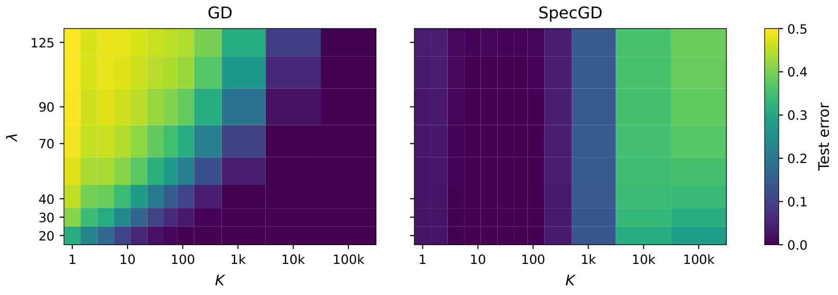
Our results show that generalization is shaped jointly by shortcut geometry and optimizer geometry: reorganizing the same memorization features across singular directions can reverse the relative performance of GD and SpecGD. Figure 3 illustrates this transition continuously as the shortcut dimension KK and strength λ\lambda vary, while additional experiments in Appendix I explore the effects of sample size, signal rank, and training time. In the dispersed setting, we further show that vanishing random correlations can qualitatively change the SpecGD limit relative to exact orthogonality. SpecGD may also interpolate and generalize after a single step while converging to a substantially worse late-stage classifier, making early stopping beneficial. On the technical side, our second-order dual analysis and dynamical selection argument may extend to other steepest-descent methods with analogous implicit-bias questions, such as SignGD. Natural extensions include higher-rank shortcuts, practical Muon variants, and nonlinear models.
Refer to caption
Figure 3: Test error vs. shortcut dimension KK and strength λ\lambda for GD and SpecGD. Parameters: n=100n=100, r=1r=1, D=105D=10^{5}, ρ=0.45\rho=0.45, ‖S‖F=‖S‖1=1||S||_{F}=||S||_{1}=1, T=104T=10^{4}, η=10−2\eta=10^{-2}.

Acknowledgements

AI use statement

We used generative AI tools to assist with mathematical derivations and proof checking, numerical code development and debugging, manuscript editing, and exploratory discussions. All AI-assisted outputs, including mathematical claims and experiments, were independently verified by the authors, who take full responsibility for the final content of the paper.

References

  • AI et al. (2025) E. AI, :, I. Shah, A. M. Polloreno, K. Stratos, P. Monk, A. Chaluvaraju, A. Hojel, A. Ma, A. Thomas, A. Tanwer, D. J. Shah, K. Nguyen, K. Smith, M. Callahan, M. Pust, M. Parmar, P. Rushton, P. Mazarakis, R. Kapila, S. Srivastava, S. Singla, T. Romanski, Y. Vanjani, and A. Vaswani Practical efficiency of muon for pretraining. External Links: 2505.02222 Cited by: §1.
  • Arpit et al. (2017) D. Arpit, S. Jastrzębski, N. Ballas, D. Krueger, E. Bengio, M. S. Kanwal, T. Maharaj, A. Fischer, A. Courville, Y. Bengio, and S. Lacoste-Julien A closer look at memorization in deep networks. In Proceedings of the 34th International Conference on Machine Learning, D. Precup and Y. W. Teh (Eds.), Proceedings of Machine Learning Research, Vol. 70, pp. 233–242. Cited by: §1.2.
  • Bombari and Mondelli (2024) S. Bombari and M. Mondelli How spurious features are memorized: precise analysis for random and NTK features. In Proceedings of the 41st International Conference on Machine Learning, R. Salakhutdinov, Z. Kolter, K. Heller, A. Weller, N. Oliver, J. Scarlett, and F. Berkenkamp (Eds.), Proceedings of Machine Learning Research, Vol. 235, pp. 4267–4299. Cited by: §1.2.
  • Braun et al. (2026) G. Braun, H. Bao, W. Huang, and M. Imaizumi Spectral gradient descent mitigates anisotropy-driven misalignment: a case study in phase retrieval. In Forty-third International Conference on Machine Learning, Cited by: §1.
  • Cai et al. (2025) Y. Cai, K. Zhou, J. Wu, S. Mei, M. Lindsey, and P. Bartlett Implicit bias of gradient descent for non-homogeneous deep networks. In Forty-second International Conference on Machine Learning, External Links: Link Cited by: Appendix A.
  • Cao et al. (2021) Y. Cao, Q. Gu, and M. Belkin Risk bounds for over-parameterized maximum margin classification on sub-gaussian mixtures. In Advances in Neural Information Processing Systems, M. Ranzato, A. Beygelzimer, Y. Dauphin, P.S. Liang, and J. W. Vaughan (Eds.), Vol. 34, pp. 8407–8418. Cited by: §1.2, §2.
  • Casella and Berger (2002) G. Casella and R. L. Berger Statistical inference. 2 edition, Duxbury. Cited by: §C.3.
  • Chatterji and Long (2021) N. S. Chatterji and P. M. Long Finite-sample analysis of interpolating linear classifiers in the overparameterized regime. Journal of Machine Learning Research 22 (129), pp. 1–30. Cited by: §1.2, §2.
  • Chen et al. (2026) L. Chen, J. Li, and Q. Liu Muon optimizes under spectral norm constraints. Transactions on Machine Learning Research. External Links: ISSN 2835-8856 Cited by: Appendix A.
  • Dragutinović et al. (2026) S. Dragutinović, Y. Zhang, and R. Ranganath To use or not to use muon: how simplicity bias in optimizers matters. External Links: 2603.00742 Cited by: §1.
  • Fan et al. (2025) C. Fan, M. Schmidt, and C. Thrampoulidis Implicit bias of spectral descent and muon on multiclass separable data. In The Thirty-ninth Annual Conference on Neural Information Processing Systems, Cited by: §1.2, §1, §2, §4, Remark 1.
  • Frei et al. (2023) S. Frei, G. Vardi, P. Bartlett, and N. Srebro Benign overfitting in linear classifiers and leaky ReLU networks from KKT conditions for margin maximization. In Proceedings of the Thirty-Sixth Conference on Learning Theory, Proceedings of Machine Learning Research, Vol. 195, pp. 3173–3228. Cited by: §1.2, §2.
  • Gronich and Vardi (2026) E. Gronich and G. Vardi The implicit bias of adam and muon on smooth homogeneous neural networks. In Forty-third International Conference on Machine Learning, Cited by: Appendix A.
  • Gunasekar et al. (2018) S. Gunasekar, J. Lee, D. Soudry, and N. Srebro Characterizing implicit bias in terms of optimization geometry. In Proceedings of the 35th International Conference on Machine Learning, Proceedings of Machine Learning Research, Vol. 80, pp. 1832–1841. Cited by: Appendix E, §1.2, §3.2, Remark 1.
  • Hashimoto et al. (2026) I. Hashimoto, S. Volgushev, and P. Zwiernik Universality of benign overfitting in binary linear classification. External Links: 2501.10538 Cited by: §1.2.
  • Hashimoto (2026) I. Hashimoto Directional convergence, benign overfitting of gradient descent in leaky reLU two-layer neural networks. In The Fourteenth International Conference on Learning Representations, Cited by: §1.2, §2.
  • Ji and Telgarsky (2020) Z. Ji and M. Telgarsky Directional convergence and alignment in deep learning. In Advances in Neural Information Processing Systems, H. Larochelle, M. Ranzato, R. Hadsell, M.F. Balcan, and H. Lin (Eds.), Vol. 33, pp. 17176–17186. External Links: Link Cited by: Appendix A.
  • Ji and Telgarsky (2021) Z. Ji and M. Telgarsky Characterizing the implicit bias via a primal-dual analysis. In Proceedings of the 32nd International Conference on Algorithmic Learning Theory, V. Feldman, K. Ligett, and S. Sabato (Eds.), Proceedings of Machine Learning Research, Vol. 132, pp. 772–804. External Links: Link Cited by: §1.2.
  • Jiang et al. (2024) J. Jiang, W. Huang, M. Zhang, T. Suzuki, and L. Nie Unveil benign overfitting for transformer in vision: training dynamics, convergence, and generalization. In The Thirty-eighth Annual Conference on Neural Information Processing Systems, Cited by: Appendix A.
  • Jordan et al. (2024) K. Jordan, Y. Jin, V. Boza, Y. Jiacheng, F. Cesista, L. Newhouse, and J. Bernstein Muon: an optimizer for hidden layers in neural networks. External Links: Link Cited by: §1.
  • Kang et al. (2026) C. Kang, J. Yun, B. Shin, Y. Cho, and C. Yun Uniform spectral growth and convergence of muon in lora-style matrix factorization. External Links: 2602.06385 Cited by: §1.
  • Kingma and Ba (2015) D. P. Kingma and J. Ba Adam: A method for stochastic optimization. In 3rd International Conference on Learning Representations, ICLR 2015, San Diego, CA, USA, May 7-9, 2015, Conference Track Proceedings, Y. Bengio and Y. LeCun (Eds.), Cited by: §1.
  • Laurent and Massart (2000) B. Laurent and P. Massart Adaptive estimation of a quadratic functional by model selection. The Annals of Statistics 28 (5), pp. 1302–1338. External Links: Document Cited by: §H.2.
  • Levy (2006) E. Levy Why do partitions occur in faa di bruno’s chain rule for higher derivatives?. arXiv preprint math/0602183. External Links: math/0602183 Cited by: §C.1.
  • Li et al. (2026) J. Li, X. Tang, and D. Zou The implicit bias of steepest descent with mini-batch stochastic gradient. In Forty-third International Conference on Machine Learning, Cited by: Appendix A.
  • Liu et al. (2025) J. Liu, J. Su, X. Yao, Z. Jiang, G. Lai, Y. Du, Y. Qin, W. Xu, E. Lu, J. Yan, Y. Chen, H. Zheng, Y. Liu, S. Liu, B. Yin, W. He, H. Zhu, Y. Wang, J. Wang, M. Dong, Z. Zhang, Y. Kang, H. Zhang, X. Xu, Y. Zhang, Y. Wu, X. Zhou, and Z. Yang Muon is scalable for llm training. External Links: 2502.16982 Cited by: §1.
  • Lyu and Li (2020) K. Lyu and J. Li Gradient descent maximizes the margin of homogeneous neural networks. In International Conference on Learning Representations, External Links: Link Cited by: Appendix A.
  • Ma et al. (2026) J. Ma, Y. Huang, Y. Chi, and Y. Chen Preconditioning benefits of spectral orthogonalization in muon. External Links: 2601.13474 Cited by: §1.
  • Magen et al. (2025) R. Magen, S. Shang, Z. Xu, S. Frei, W. Hu, and G. Vardi Benign overfitting in single-head attention. In Advances in Neural Information Processing Systems, Vol. 38. External Links: Link Cited by: Appendix A, §1.2.
  • Minsker and Wei (2019) S. Minsker and X. Wei Moment inequalities for matrix-valued U-statistics of order 2. Electronic Journal of Probability 24, pp. 1–26. Cited by: §C.4, Theorem 6.
  • Ruan et al. (2026) T. Ruan, F. Zhang, S. Wang, and S. Zhang Muon learns more robust and transferable features than adam. External Links: 2606.09658 Cited by: §1.
  • Sakamoto and Sato (2025) K. Sakamoto and I. Sato Benign overfitting in token selection of attention mechanism. In Proceedings of the 42nd International Conference on Machine Learning, A. Singh, M. Fazel, D. Hsu, S. Lacoste-Julien, F. Berkenkamp, T. Maharaj, K. Wagstaff, and J. Zhu (Eds.), Proceedings of Machine Learning Research, Vol. 267, pp. 52644–52727. Cited by: Appendix A.
  • Schechtman and Schreuder (2025) S. Schechtman and N. Schreuder The late-stage training dynamics of (stochastic) subgradient descent on homogeneous neural networks. In Proceedings of Thirty Eighth Conference on Learning Theory, N. Haghtalab and A. Moitra (Eds.), Proceedings of Machine Learning Research, Vol. 291, pp. 5143–5172. External Links: Link Cited by: Appendix A.
  • Shamir (2022) O. Shamir The implicit bias of benign overfitting. In Proceedings of Thirty Fifth Conference on Learning Theory, Vol. 178, pp. 448–478. Cited by: Appendix A, §2.
  • Soudry et al. (2018) D. Soudry, E. Hoffer, M. S. Nacson, S. Gunasekar, and N. Srebro The implicit bias of gradient descent on separable data. J. Mach. Learn. Res. 19 (1), pp. 2822–2878. Cited by: §1.2, §3.2.
  • Vardi (2022) G. Vardi On the implicit bias in deep-learning algorithms. External Links: 2208.12591, Link Cited by: Appendix A.
  • Vasudeva et al. (2026) B. Vasudeva, P. Deora, Y. Zhao, V. Sharan, and C. Thrampoulidis How muon’s spectral design benefits generalization: a study on imbalanced data. In The Fourteenth International Conference on Learning Representations, Cited by: §1.
  • Vershynin (2026) R. Vershynin High-dimensional probability: an introduction with applications in data science. 2 edition, Cambridge University Press. Cited by: §C.3, §H.2, §H.2, §H.2.
  • Wang and Thrampoulidis (2022) K. Wang and C. Thrampoulidis Binary classification of gaussian mixtures: abundance of support vectors, benign overfitting, and regularization. SIAM Journal on Mathematics of Data Science 4 (1), pp. 260–284. External Links: Document, Link Cited by: §1.2, §2.
  • Xu and Gu (2023) X. Xu and Y. Gu Benign overfitting of non-smooth neural networks beyond lazy training. In Proceedings of The 26th International Conference on Artificial Intelligence and Statistics, F. Ruiz, J. Dy, and J. van de Meent (Eds.), Proceedings of Machine Learning Research, Vol. 206, pp. 11094–11117. External Links: Link Cited by: Appendix A, §2.
  • Zhang et al. (2017) C. Zhang, S. Bengio, M. Hardt, B. Recht, and O. Vinyals Understanding deep learning requires rethinking generalization. In International Conference on Learning Representations, Cited by: §1.2.

Appendix A Additional related work

Additional implicit-bias literature.

Implicit bias has been studied as a possible mechanism for understanding generalization in overparameterized models [Vardi, 2022], including margin-maximizing behavior in homogeneous and nearly homogeneous neural networks [Lyu and Li, 2020, Ji and Telgarsky, 2020, Cai et al., 2025, Schechtman and Schreuder, 2025]. Recent work also studies implicit bias and optimization geometry for Muon and related spectral methods [Gronich and Vardi, 2026, Li et al., 2026, Chen et al., 2026].

Additional benign-overfitting literature.

Further results on benign overfitting in classification include [Shamir, 2022, Xu and Gu, 2023], while recent work studies analogous phenomena in attention models and Transformers [Magen et al., 2025, Sakamoto and Sato, 2025, Jiang et al., 2024].

Appendix B Directional convergence via dual framework

In this section, we present our dual framework for establishing directional convergence, separating the general dual-dynamical mechanism from the model-specific arguments required to identify and control the limiting dual solution.

Throughout, set Ni:=y~i​𝒖i​𝒗i⊤N_{i}:=\tilde{y}_{i}\boldsymbol{u}_{i}\boldsymbol{v}_{i}^{\top} and Ai:=y~i​Xi=ξi​S+λ​NiA_{i}:=\tilde{y}_{i}X_{i}=\xi_{i}S+\lambda N_{i}.

B.1 Block geometry

Choose orthonormal complements P⟂P_{\perp} and Q⟂Q_{\perp}. Define 𝒮:={P​M​Q⊤:M∈ℝr×r}\mathcal{S}:=\{PMQ^{\top}:M\in\mathbb{R}^{r\times r}\} and 𝒩:={P⟂​N​Q⟂⊤:N∈ℝD×D}\mathcal{N}:=\{P_{\perp}NQ_{\perp}^{\top}:N\in\mathbb{R}^{D\times D}\}. Then S∈𝒮S\in\mathcal{S}, every Ni∈𝒩N_{i}\in\mathcal{N}, and matrices in 𝒮\mathcal{S} and 𝒩\mathcal{N} have mutually orthogonal row and column spaces.

Lemma 1 (Polar factor and Schatten 1-norm of orthogonal blocks).

For every c∈ℝc\in\mathbb{R} and Z∈𝒩Z\in\mathcal{N}, Polar⁡(c​S+λ​Z)=sgn⁡(c)​PS+Polar⁡(Z)\pol(cS+\lambda Z)=\operatorname{sgn}(c)P_{S}+\pol(Z), where the first term is zero when c=0c=0. Moreover, ‖c​S+λ​Z‖1=|c|​s+λ​‖Z‖1\|cS+\lambda Z\|_{1}=|c|s+\lambda\|Z\|_{1}.

Proof.

Relative to the orthogonal row and column bases [P​P⟂][P\ P_{\perp}] and [Q​Q⟂][Q\ Q_{\perp}], the matrix is block diagonal:

(c​Σ00λ​Z¯).\begin{pmatrix}c\Sigma&0\\ 0&\lambda\overline{Z}\end{pmatrix}.

The singular values are the union of the singular values of the two blocks, which proves Schatten-1-norm additivity. Combining the compact singular value decompositions of the two blocks gives the polar-factor identity. ∎

B.2 Primal–dual reduction

The spectral max-margin value is γ⋆:=max‖W‖op≤1⁡mini∈[n]​⟨W,Ai⟩F\gamma_{\star}:=\max_{\|W\|_{\mathrm{op}}\leq 1}\min_{i\in[n]}\left\langle W,A_{i}\right\rangle_{F}.

Proposition 2 (Exact dual and one-dimensional reduction).

We have

γ⋆=min𝜶∈Δn⁡F⁡(𝜶),F⁡(𝜶):=‖∑i=1nαi​Ai‖1.\gamma_{\star}=\min_{\boldsymbol{\alpha}\in\Delta_{n}}F(\boldsymbol{\alpha}),\qquad F(\boldsymbol{\alpha}):=\left\|\sum_{i=1}^{n}\alpha_{i}A_{i}\right\|_{1}.

If q⁡(𝛂):=∑i∈I+αi,Z⁡(𝛂):=∑i=1nαi​Niq(\boldsymbol{\alpha}):=\sum_{i\in I_{+}}\alpha_{i},\quad Z(\boldsymbol{\alpha}):=\sum_{i=1}^{n}\alpha_{i}N_{i}, then F⁡(𝛂)=2​s​|q⁡(𝛂)−12|+λ​‖Z⁡(𝛂)‖1F(\boldsymbol{\alpha})=2s\left|q(\boldsymbol{\alpha})-\frac{1}{2}\right|+\lambda\|Z(\boldsymbol{\alpha})\|_{1}. Consequently,

γ⋆=minq∈[0,1]⁡{2​s​|q−12|+λ​ψ​(q)},\gamma_{\star}=\min_{q\in[0,1]}\left\{2s\left|q-\frac{1}{2}\right|+\lambda\psi(q)\right\}, (B.1)

where

ψ⁡(q):=min𝜶∈Δnq⁡(𝜶)=q⁡‖Z⁡(𝜶)‖1.\psi(q):=\min_{\begin{subarray}{c}\boldsymbol{\alpha}\in\Delta_{n}\\ q(\boldsymbol{\alpha})=q\end{subarray}}\|Z(\boldsymbol{\alpha})\|_{1}.

The function ψ\psi is convex.

Proof.

For every WW, mini⁡⟨W,Ai⟩F=min⁡∑i𝜶∈Δn⁡αi​⟨W,Ai⟩F\min_{i}\left\langle W,A_{i}\right\rangle_{F}=\min_{\boldsymbol{\alpha}\in\Delta_{n}}\sum_{i}\alpha_{i}\left\langle W,A_{i}\right\rangle_{F}. Sion’s minimax theorem gives γ⋆=min𝜶∈Δn⁡max‖W‖op≤1​⟨W,∑iαi​Ai⟩F\gamma_{\star}=\min_{\boldsymbol{\alpha}\in\Delta_{n}}\max_{\|W\|_{\mathrm{op}}\leq 1}\left\langle W,\sum_{i}\alpha_{i}A_{i}\right\rangle_{F}. Spectral–Schatten-1 duality yields max‖W‖op≤1⁡⟨W,M⟩F=‖M‖1\max_{\|W\|_{\mathrm{op}}\leq 1}\left\langle W,M\right\rangle_{F}=\|M\|_{1}. This proves the first identity.

Furthermore, ∑i𝜶i​Ai=(2​q​(𝜶)−1)​S+λ​Z​(𝜶)\sum_{i}\boldsymbol{\alpha}_{i}A_{i}=(2q(\boldsymbol{\alpha})-1)S+\lambda Z(\boldsymbol{\alpha}), so Lemma 1 proves the decomposition and the reduced problem.

To prove convexity of ψ\psi, let q0,q1∈[0,1]q_{0},q_{1}\in[0,1], choose feasible 𝜶(0),𝜶(1)\boldsymbol{\alpha}^{(0)},\boldsymbol{\alpha}^{(1)}, and let t∈[0,1]t\in[0,1]. Then t​𝜶(1)+(1−t)​𝜶(0)t\boldsymbol{\alpha}^{(1)}+(1-t)\boldsymbol{\alpha}^{(0)} is feasible for t​q1+(1−t)​q0tq_{1}+(1-t)q_{0}, and convexity of the Schatten 1-norm gives ψ⁡(t​q1+(1−t)​q0)≤t​‖Z⁡(𝜶(1))‖1+(1−t)​‖Z⁡(𝜶(0))‖1\psi(tq_{1}+(1-t)q_{0})\leq t\|Z(\boldsymbol{\alpha}^{(1)})\|_{1}+(1-t)\|Z(\boldsymbol{\alpha}^{(0)})\|_{1}. Taking infima proves convexity. ∎

B.3 Exact dual dynamics

Define

αi,k:=exp⁡(−⟨WkSpecGD,Ai⟩F)∑j=1nexp⁡(−⟨WkSpecGD,Aj⟩F).\alpha_{i,k}:=\frac{\exp(-\left\langle W_{k}^{\mathrm{SpecGD}},A_{i}\right\rangle_{F})}{\sum_{j=1}^{n}\exp(-\left\langle W_{k}^{\mathrm{SpecGD}},A_{j}\right\rangle_{F})}. (B.2)

Then 𝜶k∈int⁡(Δn)\boldsymbol{\alpha}_{k}\in\operatorname{int}(\Delta_{n}).

Set M⁡(𝜶):=∑iαi​AiM(\boldsymbol{\alpha}):=\sum_{i}\alpha_{i}A_{i}. Since −∇ℒ​(WkSpecGD)=ℒ⁡(WkSpecGD)​M​(𝜶k)-\nabla\mathcal{L}(W_{k}^{\mathrm{SpecGD}})=\mathcal{L}(W_{k}^{\mathrm{SpecGD}})M(\boldsymbol{\alpha}_{k}), we have Gk:=Polar⁡(−∇ℒ​(WkSpecGD))=Polar⁡(M⁡(𝜶k))G_{k}:=\pol(-\nabla\mathcal{L}(W_{k}^{\mathrm{SpecGD}}))=\pol(M(\boldsymbol{\alpha}_{k})). Define gi,k:=⟨Gk,Ai⟩Fg_{i,k}:=\left\langle G_{k},A_{i}\right\rangle_{F}.

Lemma 2 (Exponentiated-gradient recursion).

For every i,ki,k, αi,k+1=αi,k​exp⁡(−ηk​gi,k)∑jαj,k​exp⁡(−ηk​gj,k)\alpha_{i,k+1}=\frac{\alpha_{i,k}\exp(-\eta_{k}g_{i,k})}{\sum_{j}\alpha_{j,k}\exp(-\eta_{k}g_{j,k})}. Moreover, 𝐠k:=(g1,k,…,gn,k)∈∂F⁡(𝛂k),‖gk‖∞≤s+λ\boldsymbol{g}_{k}:=(g_{1,k},\ldots,g_{n,k})\in\partial F(\boldsymbol{\alpha}_{k}),\quad\|g_{k}\|_{\infty}\leq s+\lambda.

Proof.

The recursion follows directly from exp⁡(−⟨Wk+1SpecGD,Ai⟩F)=exp⁡(−⟨WkSpecGD,Ai⟩F)​e−ηk​gi,k\exp(-\left\langle W_{k+1}^{\mathrm{SpecGD}},A_{i}\right\rangle_{F})=\exp(-\left\langle W_{k}^{\mathrm{SpecGD}},A_{i}\right\rangle_{F})e^{-\eta_{k}g_{i,k}}.

Because Gk=Polar⁡(M⁡(𝜶k))G_{k}=\pol(M(\boldsymbol{\alpha}_{k})), we have ‖Gk‖op≤1,⟨Gk,M⁡(𝜶k)⟩F=‖M⁡(𝜶k)‖1\|G_{k}\|_{\mathrm{op}}\leq 1,\quad\left\langle G_{k},M(\boldsymbol{\alpha}_{k})\right\rangle_{F}=\|M(\boldsymbol{\alpha}_{k})\|_{1}. Thus Gk∈∂∥⋅∥1(M(𝜶k))G_{k}\in\partial\|\cdot\|_{1}(M(\boldsymbol{\alpha}_{k})). For 𝜷∈Δn\boldsymbol{\beta}\in\Delta_{n}, F⁡(𝜷)≥F⁡(𝜶k)+∑i(βi−αi,k)​⟨Gk,Ai⟩FF(\boldsymbol{\beta})\geq F(\boldsymbol{\alpha}_{k})+\sum_{i}(\beta_{i}-\alpha_{i,k})\left\langle G_{k},A_{i}\right\rangle_{F}, which proves gk∈∂F⁡(𝜶k)g_{k}\in\partial F(\boldsymbol{\alpha}_{k}).

Finally, |gi,k|≤‖Gk‖op​‖Ai‖1≤s+λ|g_{i,k}|\leq\|G_{k}\|_{\mathrm{op}}\|A_{i}\|_{1}\leq s+\lambda by Lemma 1. ∎

B.4 Dual convergence under local growth

For 𝜶,𝜷∈int⁡(Δn)\boldsymbol{\alpha},\boldsymbol{\beta}\in\operatorname{int}(\Delta_{n}), define DKL(𝜶∥𝜷):=∑iαilogαiβiD_{\mathrm{KL}}(\boldsymbol{\alpha}\|\boldsymbol{\beta}):=\sum_{i}\alpha_{i}\log\frac{\alpha_{i}}{\beta_{i}}.

Lemma 3 (Local quadratic upper bound for relative entropy).

Let 𝛂⋆∈int⁡(Δn)\boldsymbol{\alpha}^{\star}\in\operatorname{int}(\Delta_{n}). Then there exist constants CKL>0C_{\mathrm{KL}}>0 and εKL>0\varepsilon_{\mathrm{KL}}>0 such that DKL(𝛂⋆∥𝛂)≤CKL∥𝛂−𝛂⋆∥22D_{\mathrm{KL}}(\boldsymbol{\alpha}^{\star}\|\boldsymbol{\alpha})\leq C_{\mathrm{KL}}\|\boldsymbol{\alpha}-\boldsymbol{\alpha}^{\star}\|_{2}^{2} for every 𝛂∈Δn\boldsymbol{\alpha}\in\Delta_{n} satisfying ‖𝛂−𝛂⋆‖2≤εKL\|\boldsymbol{\alpha}-\boldsymbol{\alpha}^{\star}\|_{2}\leq\varepsilon_{\mathrm{KL}}.

Proof.

Let a⋆:=mini⁡αi⋆>0a_{\star}:=\min_{i}\alpha_{i}^{\star}>0, and choose εKL≤a⋆/2\varepsilon_{\mathrm{KL}}\leq a_{\star}/2. If ‖𝜶−𝜶⋆‖2≤εKL\|\boldsymbol{\alpha}-\boldsymbol{\alpha}^{\star}\|_{2}\leq\varepsilon_{\mathrm{KL}}, then, for every ii,

αi≥αi⋆−‖𝜶−𝜶⋆‖∞≥αi⋆2.\alpha_{i}\geq\alpha_{i}^{\star}-\|\boldsymbol{\alpha}-\boldsymbol{\alpha}^{\star}\|_{\infty}\geq\frac{\alpha_{i}^{\star}}{2}. (B.3)

For fi​(x):=αi⋆​log⁡(αi⋆/x)f_{i}(x):=\alpha_{i}^{\star}\log(\alpha_{i}^{\star}/x), we have fi​(αi⋆)=0f_{i}(\alpha_{i}^{\star})=0, fi′​(αi⋆)=−1f_{i}^{\prime}(\alpha_{i}^{\star})=-1, and fi′′​(x)=αi⋆/x2f_{i}^{\prime\prime}(x)=\alpha_{i}^{\star}/x^{2}. By Taylor’s theorem, for some α~i\widetilde{\alpha}_{i} between αi\alpha_{i} and αi⋆\alpha_{i}^{\star},

fi​(αi)=−(αi−αi⋆)+12​αi⋆α~i2​(αi−αi⋆)2.f_{i}(\alpha_{i})=-(\alpha_{i}-\alpha_{i}^{\star})+\frac{1}{2}\frac{\alpha_{i}^{\star}}{\widetilde{\alpha}_{i}^{2}}(\alpha_{i}-\alpha_{i}^{\star})^{2}.

By (B.3), we have α~i≥αi⋆/2\widetilde{\alpha}_{i}\geq\alpha_{i}^{\star}/2, and hence αi⋆α~i2≤4αi⋆≤4a⋆\frac{\alpha_{i}^{\star}}{\widetilde{\alpha}_{i}^{2}}\leq\frac{4}{\alpha_{i}^{\star}}\leq\frac{4}{a_{\star}}. Summing over ii and using ∑i(αi−αi⋆)=0\sum_{i}(\alpha_{i}-\alpha_{i}^{\star})=0, we obtain

DKL(𝜶⋆∥𝜶)=∑ifi(αi)≤2a⋆∑i(αi−αi⋆)2.D_{\mathrm{KL}}(\boldsymbol{\alpha}^{\star}\|\boldsymbol{\alpha})=\sum_{i}f_{i}(\alpha_{i})\leq\frac{2}{a_{\star}}\sum_{i}(\alpha_{i}-\alpha_{i}^{\star})^{2}.

Thus the claim holds with CKL=2/a⋆C_{\mathrm{KL}}=2/a_{\star}. ∎

Definition 1 (Local relative growth).

A convex function FF has local relative growth at an interior minimizer 𝛂⋆\boldsymbol{\alpha}^{\star} if there exist r,μ>0r,\mu>0 such that F(𝛂)−F(𝛂⋆)≥μDKL(𝛂⋆∥𝛂)F(\boldsymbol{\alpha})-F(\boldsymbol{\alpha}^{\star})\geq\mu D_{\mathrm{KL}}(\boldsymbol{\alpha}^{\star}\|\boldsymbol{\alpha}) whenever DKL(𝛂⋆∥𝛂)≤rD_{\mathrm{KL}}(\boldsymbol{\alpha}^{\star}\|\boldsymbol{\alpha})\leq r.

Lemma 4 (One-step relative-entropy inequality).

If 𝛂⋆\boldsymbol{\alpha}^{\star} minimizes FF, then

DKL(𝜶⋆∥𝜶k+1)≤DKL(𝜶⋆∥𝜶k)−ηk(F(𝜶k)−F(𝜶⋆))+(s+λ)22ηk2.D_{\mathrm{KL}}(\boldsymbol{\alpha}^{\star}\|\boldsymbol{\alpha}_{k+1})\leq D_{\mathrm{KL}}(\boldsymbol{\alpha}^{\star}\|\boldsymbol{\alpha}_{k})-\eta_{k}\bigl(F(\boldsymbol{\alpha}_{k})-F(\boldsymbol{\alpha}^{\star})\bigr)+\frac{(s+\lambda)^{2}}{2}\eta_{k}^{2}.
Proof.

Let ZkEG:=∑iαi,k​e−ηk​gi,kZ_{k}^{\mathrm{EG}}:=\sum_{i}\alpha_{i,k}e^{-\eta_{k}g_{i,k}}. The exponentiated-gradient recursion gives

DKL(𝜶⋆∥𝜶k+1)−DKL(𝜶⋆∥𝜶k)=ηk⟨𝜶⋆,𝒈k⟩+logZkEG.D_{\mathrm{KL}}(\boldsymbol{\alpha}^{\star}\|\boldsymbol{\alpha}_{k+1})-D_{\mathrm{KL}}(\boldsymbol{\alpha}^{\star}\|\boldsymbol{\alpha}_{k})=\eta_{k}\langle\boldsymbol{\alpha}^{\star},\boldsymbol{g}_{k}\rangle+\log Z_{k}^{\mathrm{EG}}.

By Hoeffding’s lemma, if a random variable XX satisfies X∈[a,b]X\in[a,b] almost surely, then log⁡𝔼​eθ⁡(X−𝔼​X)≤θ2​(b−a)28\log\mathbb{E}e^{\theta(X-\mathbb{E}X)}\leq\frac{\theta^{2}(b-a)^{2}}{8}. We apply this to the finite random variable XX defined by ℙ⁡(X=gi,k)=αi,k\mathbb{P}(X=g_{i,k})=\alpha_{i,k}. Since |gi,k|=|⟨Gk,Ai⟩F|≤‖Gk‖op​‖Ai‖1≤s+λ|g_{i,k}|=|\langle G_{k},A_{i}\rangle_{F}|\leq\|G_{k}\|_{\mathrm{op}}\|A_{i}\|_{1}\leq s+\lambda, we have X∈[−B,B]X\in[-B,B], where B=s+λB=s+\lambda. Taking θ=−ηk\theta=-\eta_{k}, Hoeffding’s lemma gives log⁡ZkEG≤−ηk​⟨𝜶k,𝒈k⟩+(s+λ)22​ηk2\log Z_{k}^{\mathrm{EG}}\leq-\eta_{k}\langle\boldsymbol{\alpha}_{k},\boldsymbol{g}_{k}\rangle+\frac{(s+\lambda)^{2}}{2}\eta_{k}^{2}. Thus,

DKL(𝜶⋆∥𝜶k+1)−DKL(𝜶⋆∥𝜶k)≤ηk⟨𝜶⋆−𝜶k,𝒈k⟩+(s+λ)22ηk2.D_{\mathrm{KL}}(\boldsymbol{\alpha}^{\star}\|\boldsymbol{\alpha}_{k+1})-D_{\mathrm{KL}}(\boldsymbol{\alpha}^{\star}\|\boldsymbol{\alpha}_{k})\leq\eta_{k}\langle\boldsymbol{\alpha}^{\star}-\boldsymbol{\alpha}_{k},\boldsymbol{g}_{k}\rangle+\frac{(s+\lambda)^{2}}{2}\eta_{k}^{2}.

The subgradient inequality gives F⁡(𝜶⋆)−F⁡(𝜶k)≥⟨𝒈k,𝜶⋆−𝜶k⟩F(\boldsymbol{\alpha}^{\star})-F(\boldsymbol{\alpha}_{k})\geq\langle\boldsymbol{g}_{k},\boldsymbol{\alpha}^{\star}-\boldsymbol{\alpha}_{k}\rangle, and the conclusion follows. ∎

Theorem 5 (Dual convergence).

Suppose FF has a unique minimizer 𝛂⋆∈int⁡(Δn)\boldsymbol{\alpha}^{\star}\in\operatorname{int}(\Delta_{n}) and has local relative growth μ\mu at 𝛂⋆\boldsymbol{\alpha}^{\star}. Then 𝛂k→𝛂⋆\boldsymbol{\alpha}_{k}\to\boldsymbol{\alpha}^{\star}.

Moreover, if we further assume lim supk→∞ηk−ηk+1ηk2<μ\limsup_{k\to\infty}\frac{\eta_{k}-\eta_{k+1}}{\eta_{k}^{2}}<\mu, then ‖𝛂k−𝛂⋆‖1=O⁡(ηk)\|\boldsymbol{\alpha}_{k}-\boldsymbol{\alpha}^{\star}\|_{1}=O(\sqrt{\eta_{k}}).

Proof.

Write

dk:=DKL(𝜶⋆∥𝜶k),δk:=F(𝜶k)−F(𝜶⋆),C=(s+λ)22.d_{k}:=D_{\mathrm{KL}}(\boldsymbol{\alpha}^{\star}\|\boldsymbol{\alpha}_{k}),\qquad\delta_{k}:=F(\boldsymbol{\alpha}_{k})-F(\boldsymbol{\alpha}^{\star}),\qquad C=\frac{(s+\lambda)^{2}}{2}.

Lemma 4 gives dk+1≤dk−ηk​δk+C​ηk2d_{k+1}\leq d_{k}-\eta_{k}\delta_{k}+C\eta_{k}^{2}. Rearrangigng and summing from k=0k=0 to K−1K-1 gives

∑k=0K−1ηk​δk≤d0−dK+C​∑k=0K−1ηk2≤d0+C​∑k=0K−1ηk2.\sum_{k=0}^{K-1}\eta_{k}\delta_{k}\leq d_{0}-d_{K}+C\sum_{k=0}^{K-1}\eta_{k}^{2}\leq d_{0}+C\sum_{k=0}^{K-1}\eta_{k}^{2}.

Let τK:=∑k=0K−1ηk\tau_{K}:=\sum_{k=0}^{K-1}\eta_{k}. Dividing by τK\tau_{K}, we get

∑k=0K−1ηk​δkτK≤d0τK+C​∑k=0K−1ηk2τK.\frac{\sum_{k=0}^{K-1}\eta_{k}\delta_{k}}{\tau_{K}}\leq\frac{d_{0}}{\tau_{K}}+C\frac{\sum_{k=0}^{K-1}\eta_{k}^{2}}{\tau_{K}}.

Since ∑kηk=∞\sum_{k}\eta_{k}=\infty, we have τK→∞\tau_{K}\to\infty. Moreover, because ηk→0\eta_{k}\to 0, ∑k=0K−1ηk2∑k=0K−1ηk→0\frac{\sum_{k=0}^{K-1}\eta_{k}^{2}}{\sum_{k=0}^{K-1}\eta_{k}}\to 0. Indeed, for any ε>0\varepsilon>0, choose K0K_{0} such that ηk≤ε\eta_{k}\leq\varepsilon for every k≥K0k\geq K_{0}. Then ∑k=0K−1ηk2≤∑k=0K0−1ηk2+ε​∑k=K0K−1ηk\sum_{k=0}^{K-1}\eta_{k}^{2}\leq\sum_{k=0}^{K_{0}-1}\eta_{k}^{2}+\varepsilon\sum_{k=K_{0}}^{K-1}\eta_{k}. Dividing by τK\tau_{K} and letting K→∞K\to\infty, we obtain lim supK→∞∑k=0K−1ηk2τK≤ε\limsup_{K\to\infty}\frac{\sum_{k=0}^{K-1}\eta_{k}^{2}}{\tau_{K}}\leq\varepsilon. Since ε>0\varepsilon>0 is arbitrary, the ratio converges to zero. Therefore, ∑k=0K−1ηk​δkτK→0\frac{\sum_{k=0}^{K-1}\eta_{k}\delta_{k}}{\tau_{K}}\to 0. Since δk≥0\delta_{k}\geq 0, there exists a subsequence kj→∞k_{j}\to\infty such that δkj→0\delta_{k_{j}}\to 0. Compactness of Δn\Delta_{n}, uniqueness of the minimizer, and continuity of FF yield 𝜶kj→𝜶⋆\boldsymbol{\alpha}_{k_{j}}\to\boldsymbol{\alpha}^{\star}. Furthermore, continuity of DKL(𝜶⋆∥⋅)D_{\mathrm{KL}}(\boldsymbol{\alpha}^{\star}\|\cdot) at the interior point 𝜶⋆\boldsymbol{\alpha}^{\star} yields dkj→0d_{k_{j}}\to 0.

Let r,μr,\mu be local-growth constants. Choose a sufficiently late kjk_{j} so that dkj<r/2d_{k_{j}}<r/2 and C​ηk≤μ​r4C\eta_{k}\leq\frac{\mu r}{4} for every k≥kjk\geq k_{j}. If r/2≤dk≤rr/2\leq d_{k}\leq r, then dk+1≤dk−μ​ηk​dk+C​ηk2≤dk−μ​r4​ηk<dkd_{k+1}\leq d_{k}-\mu\eta_{k}d_{k}+C\eta_{k}^{2}\leq d_{k}-\frac{\mu r}{4}\eta_{k}<d_{k}. If dk<r/2d_{k}<r/2, then sufficiently small ηk\eta_{k} implies dk+1<rd_{k+1}<r. Thus the iterates eventually remain in the local region, where dk+1≤(1−μ​ηk)​dk+C​ηk2d_{k+1}\leq(1-\mu\eta_{k})d_{k}+C\eta_{k}^{2}.

For any ε>0\varepsilon>0, there exists KK such that k≥Kk\geq K implies C​ηk≤μ​ε/2C\eta_{k}\leq\mu\varepsilon/2 and C​ηk2≤εC\eta_{k}^{2}\leq\varepsilon since ηk→0\eta_{k}\to 0. If dk≥εd_{k}\geq\varepsilon, then

dk+1\displaystyle d_{k+1} ≤(1−μ​ηk)​dk+C​ηk2\displaystyle\leq(1-\mu\eta_{k})d_{k}+C\eta_{k}^{2}
≤dk−μ​ηk​ε+μ​ε​ηk/2\displaystyle\leq d_{k}-\mu\eta_{k}\varepsilon+\mu\varepsilon\eta_{k}/2
=dk−μ​ε​ηk/2.\displaystyle=d_{k}-\mu\varepsilon\eta_{k}/2.

Since ∑kηk=∞\sum_{k}\eta_{k}=\infty, there exists K1>KK_{1}>K such that dK1<εd_{K_{1}}<\varepsilon. Then, for k≥K1k\geq K_{1}, dk<εd_{k}<\varepsilon implies dk+1≤2​εd_{k+1}\leq 2\varepsilon due to C​ηk2≤εC\eta_{k}^{2}\leq\varepsilon while dk≥εd_{k}\geq\varepsilon implies dk+1<dkd_{k+1}<d_{k}, which by induction implies that dk≤2​εd_{k}\leq 2\varepsilon for k≥K1k\geq K_{1}.

Hence dk→0d_{k}\to 0. Pinsker’s inequality gives ‖𝜶k−𝜶⋆‖12≤2​dk→0\|\boldsymbol{\alpha}_{k}-\boldsymbol{\alpha}^{\star}\|_{1}^{2}\leq 2d_{k}\to 0.

Suppose lim supk→∞ηk−ηk+1ηk2<μ\limsup_{k\to\infty}\frac{\eta_{k}-\eta_{k+1}}{\eta_{k}^{2}}<\mu. Fix μ0\mu_{0} so that lim supk→∞ηk−ηk+1ηk2<μ0<μ\limsup_{k\to\infty}\frac{\eta_{k}-\eta_{k+1}}{\eta_{k}^{2}}<\mu_{0}<\mu. Let KK so that k≥Kk\geq K implies dk+1≤(1−μ​ηk)​dk+C​ηk2d_{k+1}\leq(1-\mu\eta_{k})d_{k}+C\eta_{k}^{2} and ηk−ηk+1ηk2≤μ0\frac{\eta_{k}-\eta_{k+1}}{\eta_{k}^{2}}\leq\mu_{0}. Set

B:=max⁡{dKηK,Cμ−μ0}.B:=\max\left\{\frac{d_{K}}{\eta_{K}},\frac{C}{\mu-\mu_{0}}\right\}.

We now claim that dk≤B​ηkd_{k}\leq B\eta_{k} holds for all k≥Kk\geq K. The claim holds at k=Kk=K by the definition of BB. Now suppose dk≤B​ηkd_{k}\leq B\eta_{k} holds. By noting that the definition of BB implies that B​μ−C≥B​μ0B\mu-C\geq B\mu_{0}, we have

dk+1\displaystyle d_{k+1} ≤(1−μ​ηk)​dk+C​ηk2\displaystyle\leq(1-\mu\eta_{k})d_{k}+C\eta_{k}^{2}
≤B⁡(1−μ​ηk)​ηk+C​ηk2=B​ηk−(B​μ−C)​ηk2\displaystyle\leq B(1-\mu\eta_{k})\eta_{k}+C\eta_{k}^{2}=B\eta_{k}-(B\mu-C)\eta_{k}^{2}
≤B​ηk−B​μ0​ηk2=B​ηk+1+B⁡(ηk−ηk+1−μ0​ηk2)≤B​ηk+1.\displaystyle\leq B\eta_{k}-B\mu_{0}\eta_{k}^{2}=B\eta_{k+1}+B(\eta_{k}-\eta_{k+1}-\mu_{0}\eta_{k}^{2})\leq B\eta_{k+1}.

Again, by Pinsker’s inequality, we obtain ‖𝜶k−𝜶⋆‖12=O⁡(ηk)\|\boldsymbol{\alpha}_{k}-\boldsymbol{\alpha}^{\star}\|_{1}^{2}=O(\eta_{k}). ∎

B.5 Which primal optimizer is selected?

Let ck:=∑iαi,k​ξi,Zk:=∑iαi,k​Nic_{k}:=\sum_{i}\alpha_{i,k}\xi_{i},\quad Z_{k}:=\sum_{i}\alpha_{i,k}N_{i}. By Lemma 1, Gk=σk​PS+Hk,σk:=sgn⁡(ck),Hk:=Polar⁡(Zk)G_{k}=\sigma_{k}P_{S}+H_{k},\quad\sigma_{k}:=\operatorname{sgn}(c_{k}),\quad H_{k}:=\pol(Z_{k}). Therefore,

WkSpecGD=(∑t<kηt​σt)​PS+∑t<kηt​Ht.W_{k}^{\mathrm{SpecGD}}=\left(\sum_{t<k}\eta_{t}\sigma_{t}\right)P_{S}+\sum_{t<k}\eta_{t}H_{t}. (B.4)

Let 𝜶⋆\boldsymbol{\alpha}^{\star} be the unique interior minimizer. Set Z⋆:=∑iαi⋆​NiZ^{\star}:=\sum_{i}\alpha_{i}^{\star}N_{i} and H⋆:=Polar⁡(Z⋆)H^{\star}:=\pol(Z^{\star}). Under DSM, since D>nD>n , U=[𝒖1,…,𝒖n]U=[\boldsymbol{u}_{1},\ldots,\boldsymbol{u}_{n}] and V^=[𝒗^1,…,𝒗^n]\widehat{V}=[\widehat{\boldsymbol{v}}_{1},\ldots,\widehat{\boldsymbol{v}}_{n}] have full column rank almost surely. Since all αi⋆>0\alpha_{i}^{\star}>0, Z⋆Z^{\star} has rank nn on its row and column spans. Lemma 43 and 42 implies that the polar factor is continuous at Z⋆Z^{\star}. Thus, 𝜶k→𝜶⋆\boldsymbol{\alpha}_{k}\to\boldsymbol{\alpha}^{\star} implies Hk→H⋆H_{k}\to H^{\star}. Under CSM, the convergence Hk→H⋆H_{k}\to H^{\star} easily follows by noting Polar⁡(Z⁡(𝜶))=∑iαi​𝒖𝒊‖∑iαi​𝒖𝒊‖2​𝒗0⊤\pol(Z(\boldsymbol{\alpha}))=\frac{\sum_{i}\alpha_{i}\boldsymbol{u_{i}}}{\|\sum_{i}\alpha_{i}\boldsymbol{u_{i}}\|_{2}}\boldsymbol{v}_{0}^{\top} and that ∑iαi​𝒖𝒊≠0\sum_{i}\alpha_{i}\boldsymbol{u_{i}}\neq 0 since 𝜶≠𝟎\boldsymbol{\alpha}\neq\boldsymbol{0}.

Define Λk:=1n+​∑i∈I+log⁡αi,k−1n−​∑i∈I−log⁡αi,k\Lambda_{k}:=\frac{1}{n_{+}}\sum_{i\in I_{+}}\log\alpha_{i,k}-\frac{1}{n_{-}}\sum_{i\in I_{-}}\log\alpha_{i,k}, and

h¯+,k:=1n+​∑i∈I+⟨Hk,Ni⟩F,h¯−,k:=1n−​∑i∈I−⟨Hk,Ni⟩F.\overline{h}_{+,k}:=\frac{1}{n_{+}}\sum_{i\in I_{+}}\left\langle H_{k},N_{i}\right\rangle_{F},\qquad\overline{h}_{-,k}:=\frac{1}{n_{-}}\sum_{i\in I_{-}}\left\langle H_{k},N_{i}\right\rangle_{F}.
Lemma 5 (Telescoping identity).

For every kk,

Λk+1−Λk=−ηk​[2​s​σk+λ⁡(h¯+,k−h¯−,k)].\Lambda_{k+1}-\Lambda_{k}=-\eta_{k}\left[2s\sigma_{k}+\lambda(\overline{h}_{+,k}-\overline{h}_{-,k})\right].
Proof.

From Lemma 2, log⁡αi,k+1=log⁡αi,k−ηk​gi,k−log⁡ZkEG\log\alpha_{i,k+1}=\log\alpha_{i,k}-\eta_{k}g_{i,k}-\log Z_{k}^{\mathrm{EG}}. The normalizing term cancels between the two group averages. Moreover, gi,k=⟨σk​PS+Hk,ξi​S+λ​Ni⟩F=s​σk​ξi+λ​⟨Hk,Ni⟩Fg_{i,k}=\left\langle\sigma_{k}P_{S}+H_{k},\xi_{i}S+\lambda N_{i}\right\rangle_{F}=s\sigma_{k}\xi_{i}+\lambda\left\langle H_{k},N_{i}\right\rangle_{F}. Substitution proves the identity. ∎

Proposition 3 (Dynamical selection formula).

Suppose Assumption A1. If the unique dual minimizer is interior and FF has local relative growth there, then WkSpecGDτk⟶a⋆​PS+H⋆\frac{W_{k}^{\mathrm{SpecGD}}}{\tau_{k}}\longrightarrow a^{\star}P_{S}+H^{\star}, where

a⋆=−λ2​s​(h+⋆−h−⋆),a^{\star}=-\frac{\lambda}{2s}(h_{+}^{\star}-h_{-}^{\star}), (B.5)

with

h+⋆:=1n+​∑i∈I+⟨H⋆,Ni⟩F,h−⋆:=1n−​∑i∈I−⟨H⋆,Ni⟩F.h_{+}^{\star}:=\frac{1}{n_{+}}\sum_{i\in I_{+}}\left\langle H^{\star},N_{i}\right\rangle_{F},\qquad h_{-}^{\star}:=\frac{1}{n_{-}}\sum_{i\in I_{-}}\left\langle H^{\star},N_{i}\right\rangle_{F}.

If we further assume Assumption A2, then we have

‖WkSpecGDτk−(a⋆​PS+H⋆)‖F=O⁡(1+∑t<kηt3/2τk)\left\|\frac{W_{k}^{\mathrm{SpecGD}}}{\tau_{k}}-(a^{\star}P_{S}+H^{\star})\right\|_{F}=O\left(\frac{1+\sum_{t<k}\eta_{t}^{3/2}}{\tau_{k}}\right)
Proof.

Theorem 5 gives 𝜶k→𝜶⋆\boldsymbol{\alpha}_{k}\to\boldsymbol{\alpha}^{\star}. Hence Λk\Lambda_{k} converges to a finite limit and Hk→H⋆H_{k}\to H^{\star}. Summing Lemma 5, dividing by τk\tau_{k}, and applying the weighted Cesàro theorem gives ∑t<kηt​σtτk→−λ2​s​(h+⋆−h−⋆)\frac{\sum_{t<k}\eta_{t}\sigma_{t}}{\tau_{k}}\to-\frac{\lambda}{2s}(h_{+}^{\star}-h_{-}^{\star}). Dividing (B.4) by τk\tau_{k} and applying weighted Cesàro convergence to HtH_{t} proves the result.

Suppose lim supk→∞ηk−ηk+1ηk2=0\limsup_{k\to\infty}\frac{\eta_{k}-\eta_{k+1}}{\eta_{k}^{2}}=0. Then, by Theorem 5 we have ‖𝜶k−𝜶⋆‖2=O⁡(ηk)\|\boldsymbol{\alpha}_{k}-\boldsymbol{\alpha}^{\star}\|_{2}=O(\sqrt{\eta_{k}}).

Since 𝜶→Polar⁡(Z⁡(𝜶))\boldsymbol{\alpha}\to\pol(Z(\boldsymbol{\alpha})) is Lipschitz continuous at 𝜶⋆\boldsymbol{\alpha}^{\star}, we have ‖Hk−H⋆‖F=O⁡(ηk)\|H_{k}-H^{\star}\|_{F}=O(\sqrt{\eta_{k}}). Then for the shortcut noise, we have

‖∑t<kηt​Htτk−H⋆‖F=O⁡(∑t<kηt3/2τk).\left\|\frac{\sum_{t<k}\eta_{t}H_{t}}{\tau_{k}}-H^{\star}\right\|_{F}=O\left(\frac{\sum_{t<k}\eta_{t}^{3/2}}{\tau_{k}}\right).

Since |h¯+,k−h+⋆|,|h¯+,k−h+⋆|=O⁡(‖Hk−H⋆‖)=O⁡(ηk)|\bar{h}_{+,k}-h_{+}^{\star}|,|\bar{h}_{+,k}-h_{+}^{\star}|=O(\|H_{k}-H^{\star}\|)=O(\sqrt{\eta_{k}}), summing Lemma 5 and dividing by τk\tau_{k} implies that

|∑t<kηt​σtτk−λ2​s​(h−⋆−h+⋆)|=O⁡(1+∑t<kηt3/2τk).\left|\frac{\sum_{t<k}\eta_{t}\sigma_{t}}{\tau_{k}}-\frac{\lambda}{2s}(h_{-}^{\star}-h_{+}^{\star})\right|=O\left(\frac{1+\sum_{t<k}\eta_{t}^{3/2}}{\tau_{k}}\right).

This gives the convergence rate for the signal direction. Combining these estimates proves the desired convergence rate. ∎

Appendix C Proof of Theorem 1

By Proposition 3, the proof of Theorem 1 is reduced to the uniqueness, interiority of the dual minimizer 𝜶⋆\boldsymbol{\alpha}^{\star} and relative local growth at 𝜶⋆\boldsymbol{\alpha}^{\star}. Under DSM, the key ingredient is the second-order expansion of ‖Z⁡(𝜶)‖1\|Z(\boldsymbol{\alpha})\|_{1}.

Throughout, set 𝒗^i:=y~i​𝒗i\hat{\boldsymbol{v}}_{i}:=\tilde{y}_{i}\boldsymbol{v}_{i}, so that Ni=𝒖i​𝒗^i⊤N_{i}=\boldsymbol{u}_{i}\hat{\boldsymbol{v}}_{i}^{\top}.

C.1 Second-order expansion

This section derives the analytic expansion that turns the nuclear norm of the noise combination into a tractable quadratic function of the weights. Recall that Z⁡(𝜶)=∑iαi​𝒖i​𝒗^i⊤Z(\boldsymbol{\alpha})=\sum_{i}\alpha_{i}\boldsymbol{u}_{i}\widehat{\boldsymbol{v}}_{i}^{\top}. Since ‖𝒖i​𝒗^i⊤‖1=1\|\boldsymbol{u}_{i}\widehat{\boldsymbol{v}}_{i}^{\top}\|_{1}=1, we have ‖Z⁡(𝜶)‖1≤∑iαi=1\|Z(\boldsymbol{\alpha})\|_{1}\leq\sum_{i}\alpha_{i}=1, where the equality holds when the noise atoms are perfectly orthogonal.

In the random model the atoms are only approximately orthogonal. The goal of this section is to establish a second-order approximation of ‖Z⁡(𝜶)‖1\|Z(\boldsymbol{\alpha})\|_{1}, which enables us to obtain a tight estimate of the noise norm gap 1−‖Z⁡(𝜶)‖11-\|Z(\boldsymbol{\alpha})\|_{1}.

Write

U=[𝒖1,…,𝒖n],V^=[𝒗^1,…,𝒗^n],Λ𝜶:=diag⁡(α1,…,αn).U=[\boldsymbol{u}_{1},\ldots,\boldsymbol{u}_{n}],\qquad\widehat{V}=[\widehat{\boldsymbol{v}}_{1},\ldots,\widehat{\boldsymbol{v}}_{n}],\qquad\Lambda_{\boldsymbol{\alpha}}:=\diag(\alpha_{1},\ldots,\alpha_{n}). (C.1)

Then Z⁡(𝜶)=U​Λ𝜶​V^⊤Z(\boldsymbol{\alpha})=U\Lambda_{\boldsymbol{\alpha}}\widehat{V}^{\top}. Also set

GU:=U⊤​U=I+ΔU,GV:=V^⊤​V^=I+ΔV,Y⁡(𝜶):=GU1/2​Λ𝜶​GV1/2.G_{U}:=U^{\top}U=I+\Delta_{U},\qquad G_{V}:=\widehat{V}^{\top}\widehat{V}=I+\Delta_{V},\qquad Y(\boldsymbol{\alpha}):=G_{U}^{1/2}\Lambda_{\boldsymbol{\alpha}}G_{V}^{1/2}. (C.2)

The matrices ΔU,ΔV\Delta_{U},\Delta_{V} are symmetric with zero diagonal.

Throughout this section, we write

𝖭⁡(Y):=1n​‖Y‖1\mathsf{N}(Y):=\frac{1}{n}\|Y\|_{1} (C.3)

for the normalized Schatten 11-norm functional on n×nn\times n matrices. On nonsingular matrices we use the factorization

𝖭=Ψ∘G,G⁡(Y):=Y⊤​Y,Ψ⁡(M):=1n​tr⁡(M1/2).\mathsf{N}=\Psi\circ G,\qquad G(Y):=Y^{\top}Y,\qquad\Psi(M):=\frac{1}{n}\operatorname{tr}(M^{1/2}). (C.4)
Lemma 6 (Uniform derivatives of the matrix square-root map).

Fix constants 0<ℓ<u<∞0<\ell<u<\infty and an integer r≥1r\geq 1. There exists a constant Cr=Cr​(ℓ,u)<∞C_{r}=C_{r}(\ell,u)<\infty such that the following holds in every dimension nn.

Let A∈ℝn×nA\in\mathbb{R}^{n\times n} be symmetric positive definite with ℓ​I⪯A⪯u​I\ell I\preceq A\preceq uI. Then the map A↦A1/2A\mapsto A^{1/2} is C∞C^{\infty} in a neighborhood of AA, and for every 1≤q≤r1\leq q\leq r, ‖dq​(A1/2)​[H1,…,Hq]‖op≤Cr​∏j=1q‖Hj‖op\left\|\mathrm{d}^{q}(A^{1/2})[H_{1},\ldots,H_{q}]\right\|_{\mathrm{op}}\leq C_{r}\prod_{j=1}^{q}\|H_{j}\|_{\mathrm{op}}. The constant CrC_{r} depends only on ℓ,u,r\ell,u,r, and not on nn.

Proof.

Choose once and for all a positively oriented contour Γ=Γℓ,u\Gamma=\Gamma_{\ell,u} contained in the right half-plane, enclosing [ℓ,u][\ell,u], and satisfying dist⁡(Γ,[ℓ,u])≥δℓ,u>0\operatorname{dist}(\Gamma,[\ell,u])\geq\delta_{\ell,u}>0. The length of Γ\Gamma, the quantity supz∈Γ|z1/2|\sup_{z\in\Gamma}|z^{1/2}|, and δℓ,u−1\delta_{\ell,u}^{-1} depend only on ℓ,u\ell,u. By the holomorphic functional calculus, A1/2=12​π​i​∫Γz1/2​(z​I−A)−1​𝑑zA^{1/2}=\frac{1}{2\pi i}\int_{\Gamma}z^{1/2}(zI-A)^{-1}\,\mathrm{d}z. Set Rz​(A):=(z​I−A)−1R_{z}(A):=(zI-A)^{-1}. Since z∈Γz\in\Gamma stays at distance at least δℓ,u\delta_{\ell,u} from the spectrum of AA, ‖Rz​(A)‖op≤δℓ,u−1\|R_{z}(A)\|_{\mathrm{op}}\leq\delta_{\ell,u}^{-1}. The resolvent derivative is d​Rz​(A)​[H]=Rz​(A)​H​Rz​(A)\mathrm{d}R_{z}(A)[H]=R_{z}(A)HR_{z}(A). Iterating this identity gives

dq(A1/2)[H1,…,Hq]=12​π​i∫Γz1/2∑π∈SqRz(A)Hπ⁡(1)Rz(A)⋯Hπ⁡(q)Rz(A)dz.\mathrm{d}^{q}(A^{1/2})[H_{1},\ldots,H_{q}]=\frac{1}{2\pi i}\int_{\Gamma}z^{1/2}\sum_{\pi\in S_{q}}R_{z}(A)H_{\pi(1)}R_{z}(A)\cdots H_{\pi(q)}R_{z}(A)\,\mathrm{d}z.

Therefore,

‖dq​(A1/2)​[H1,…,Hq]‖op\displaystyle\left\|\mathrm{d}^{q}(A^{1/2})[H_{1},\ldots,H_{q}]\right\|_{\mathrm{op}} ≤length⁡(Γ)2​π​supz∈Γ|z1/2|​q!​δℓ,u−(q+1)​∏j=1q‖Hj‖op.\displaystyle\leq\frac{\operatorname{length}(\Gamma)}{2\pi}\sup_{z\in\Gamma}|z^{1/2}|\,q!\,\delta_{\ell,u}^{-(q+1)}\prod_{j=1}^{q}\|H_{j}\|_{\mathrm{op}}.

The right-hand side depends only on ℓ,u,q\ell,u,q, not on nn. Taking the maximum over 1≤q≤r1\leq q\leq r proves the claim. ∎

The following is the standard partition form of Faà di Bruno’s formula for Fréchet derivatives; see, for example, Levy [2006].

Lemma 7 (Faà di Bruno formula for Fréchet derivatives).

Let X,Y,ZX,Y,Z be finite-dimensional normed vector spaces. Let U⊂XU\subset X and V⊂YV\subset Y be open sets, and let G:U→V,F:V→ZG:U\to V,\quad F:V\to Z be CqC^{q}. Let 𝒫q\mathcal{P}_{q} denote the set of all partitions of {1,…,q}\{1,\ldots,q\}. For a block B⊂{1,…,q}B\subset\{1,\ldots,q\}, define GB(x):=d|B|G(x)[hi:i∈B]G_{B}(x):=\mathrm{d}^{|B|}G(x)[h_{i}:i\in B], where the directions are taken in increasing order of their indices. Then

dq​(F∘G)​(x)​[h1,…,hq]=∑π∈𝒫qd|π|​F​(G⁡(x))​[GB1​(x),…,GBm​(x)],\mathrm{d}^{q}(F\circ G)(x)[h_{1},\ldots,h_{q}]=\sum_{\pi\in\mathcal{P}_{q}}\mathrm{d}^{|\pi|}F(G(x))\left[G_{B_{1}}(x),\ldots,G_{B_{m}}(x)\right],

where π={B1,…,Bm}\pi=\{B_{1},\ldots,B_{m}\} and |π|=m|\pi|=m. Since the higher derivatives are symmetric, the order of the blocks and the order inside each block are immaterial.

Equivalently, the qq-th derivative of a composition is obtained by summing over all ways of grouping the directions {h1,…,hq}\{h_{1},\ldots,h_{q}\}: each block BB is first inserted into the derivative d|B|​G​(x)\mathrm{d}^{|B|}G(x), and the resulting outputs are then inserted into the derivative of FF whose order is the number of blocks.

Lemma 8 (Composition of uniformly bounded derivatives).

Let X,Y,ZX,Y,Z be normed vector spaces, and let G:U⊂X→Y,F:V⊂Y→ZG:U\subset X\to Y,\quad F:V\subset Y\to Z be CrC^{r} maps with G⁡(U)⊂VG(U)\subset V. Suppose that for every 1≤m≤r1\leq m\leq r, there exist constants Am,Bm<∞A_{m},B_{m}<\infty such that ‖dm​F​(y)​[u1,…,um]‖Z≤Am​∏j=1m‖uj‖Y\|\mathrm{d}^{m}F(y)[u_{1},\ldots,u_{m}]\|_{Z}\leq A_{m}\prod_{j=1}^{m}\|u_{j}\|_{Y} for all y∈Vy\in V, and ‖dm​G​(x)​[h1,…,hm]‖Y≤Bm​∏j=1m‖hj‖X\|\mathrm{d}^{m}G(x)[h_{1},\ldots,h_{m}]\|_{Y}\leq B_{m}\prod_{j=1}^{m}\|h_{j}\|_{X} for all x∈Ux\in U. Then, for every 1≤q≤r1\leq q\leq r, ‖dq​(F∘G)​(x)​[h1,…,hq]‖Z≤Cq​∏j=1q‖hj‖X\|\mathrm{d}^{q}(F\circ G)(x)[h_{1},\ldots,h_{q}]\|_{Z}\leq C_{q}\prod_{j=1}^{q}\|h_{j}\|_{X}, where one may take Cq:=∑π∈𝒫qA|π|​∏B∈πB|B|C_{q}:=\sum_{\pi\in\mathcal{P}_{q}}A_{|\pi|}\prod_{B\in\pi}B_{|B|}. In particular, CqC_{q} depends only on q,A1,…,Aq,B1,…,Bqq,\quad A_{1},\ldots,A_{q},\quad B_{1},\ldots,B_{q}.

Proof.

By Faà di Bruno’s formula,

dq​(F∘G)​(x)​[h1,…,hq]=∑π∈𝒫qd|π|​F​(G⁡(x))​[GB1​(x),…,GBm​(x)],\mathrm{d}^{q}(F\circ G)(x)[h_{1},\ldots,h_{q}]=\sum_{\pi\in\mathcal{P}_{q}}\mathrm{d}^{|\pi|}F(G(x))\left[G_{B_{1}}(x),\ldots,G_{B_{m}}(x)\right],

where π={B1,…,Bm}\pi=\{B_{1},\ldots,B_{m}\}, |π|=m|\pi|=m, and GB(x):=d|B|G(x)[hi:i∈B]G_{B}(x):=\mathrm{d}^{|B|}G(x)[h_{i}:i\in B]. For a fixed partition π\pi, the assumptions give

‖d|π|​F​(G⁡(x))​[GB1​(x),…,GBm​(x)]‖Z≤A|π|​∏B∈π‖GB​(x)‖Y.\left\|\mathrm{d}^{|\pi|}F(G(x))\left[G_{B_{1}}(x),\ldots,G_{B_{m}}(x)\right]\right\|_{Z}\leq A_{|\pi|}\prod_{B\in\pi}\|G_{B}(x)\|_{Y}.

Moreover, ‖GB​(x)‖Y≤B|B|​∏i∈B‖hi‖X\|G_{B}(x)\|_{Y}\leq B_{|B|}\prod_{i\in B}\|h_{i}\|_{X}. Hence the contribution of π\pi is bounded by A|π|​∏B∈πB|B|​∏j=1q‖hj‖XA_{|\pi|}\prod_{B\in\pi}B_{|B|}\prod_{j=1}^{q}\|h_{j}\|_{X}. Summing over all partitions gives the claim. ∎

Lemma 9 (Dimension-uniform derivatives of the normalized Schatten 11-norm).

Fix constants 0<a<b<∞0<a<b<\infty and an integer r≥1r\geq 1. There exists a constant Cr<∞C_{r}<\infty, depending only on a,b,ra,b,r, such that the following holds for every dimension nn.

Let Y∈ℝn×nY\in\mathbb{R}^{n\times n} satisfy a≤σmin​(Y)≤‖Y‖op≤ba\leq\sigma_{\min}(Y)\leq\|Y\|_{\mathrm{op}}\leq b. For 𝖭\mathsf{N} defined in (C.3), equivalently 𝖭⁡(Y)=1n​tr⁡((Y⊤​Y)1/2)\mathsf{N}(Y)=\frac{1}{n}\operatorname{tr}\bigl((Y^{\top}Y)^{1/2}\bigr), 𝖭\mathsf{N} is C∞C^{\infty} in a neighborhood of YY, and for every 1≤q≤r1\leq q\leq r, |dq​𝖭​(Y)​[E1,…,Eq]|≤Cr​∏j=1q‖Ej‖op\left|\mathrm{d}^{q}\mathsf{N}(Y)[E_{1},\ldots,E_{q}]\right|\leq C_{r}\prod_{j=1}^{q}\|E_{j}\|_{\mathrm{op}}. In particular, the constant is independent of nn.

Proof.

Recall the factorization (C.4). On the set of symmetric positive-definite matrices whose spectra lie in [a2,b2][a^{2},b^{2}], Lemma 6 implies that, for each 1≤m≤r1\leq m\leq r, there is a constant Km​(a,b)K_{m}(a,b), independent of nn, such that ‖dm​(M1/2)​[H1,…,Hm]‖op≤Km​(a,b)​∏j=1m‖Hj‖op\left\|\mathrm{d}^{m}(M^{1/2})[H_{1},\ldots,H_{m}]\right\|_{\mathrm{op}}\leq K_{m}(a,b)\prod_{j=1}^{m}\|H_{j}\|_{\mathrm{op}}. Since 1n​|tr⁡(L)|≤‖L‖op\frac{1}{n}|\operatorname{tr}(L)|\leq\|L\|_{\mathrm{op}}, it follows that |dm​Ψ​(M)​[H1,…,Hm]|≤Km​(a,b)​∏j=1m‖Hj‖op\left|\mathrm{d}^{m}\Psi(M)[H_{1},\ldots,H_{m}]\right|\leq K_{m}(a,b)\prod_{j=1}^{m}\|H_{j}\|_{\mathrm{op}}.

By (C.4), it remains to control the derivatives of G⁡(Y)=Y⊤​YG(Y)=Y^{\top}Y. On the region ‖Y‖op≤b\|Y\|_{\mathrm{op}}\leq b, the map GG satisfies d​G​(Y)​[E]=Y⊤​E+E⊤​Y,‖d​G​(Y)​[E]‖op≤2​b​‖E‖op\mathrm{d}G(Y)[E]=Y^{\top}E+E^{\top}Y,\quad\|\mathrm{d}G(Y)[E]\|_{\mathrm{op}}\leq 2b\|E\|_{\mathrm{op}}, and

d2​G​(Y)​[E1,E2]=E1⊤​E2+E2⊤​E1,‖d2​G​(Y)​[E1,E2]‖op≤2​‖E1‖op​‖E2‖op.\mathrm{d}^{2}G(Y)[E_{1},E_{2}]=E_{1}^{\top}E_{2}+E_{2}^{\top}E_{1},\qquad\|\mathrm{d}^{2}G(Y)[E_{1},E_{2}]\|_{\mathrm{op}}\leq 2\|E_{1}\|_{\mathrm{op}}\|E_{2}\|_{\mathrm{op}}.

Moreover, dm​G=0\mathrm{d}^{m}G=0 for m≥3m\geq 3. Therefore the derivatives of GG up to order rr are bounded by constants depending only on bb and the derivative order. Applying Lemma 8 to the factorization (C.4) gives the desired bound. All constants depend only on a,b,ra,b,r, and not on nn. ∎

Lemma 10 (Rank-sensitive derivatives of the normalized Schatten 11-norm).

Fix constants 0<a<b<∞0<a<b<\infty and an integer r≥1r\geq 1. Consider 𝖭\mathsf{N}, defined in (C.3), on the set of matrices satisfying a≤σmin​(Y)≤‖Y‖op≤ba\leq\sigma_{\min}(Y)\leq\|Y\|_{\mathrm{op}}\leq b. For every 1≤q≤r1\leq q\leq r, there is a constant Cq=Cq​(a,b)<∞C_{q}=C_{q}(a,b)<\infty, independent of nn, such that the following bounds hold.

First, if one direction, say E1E_{1}, is measured in Schatten 11-norm and the remaining directions are measured in operator norm, then

|dq​𝖭​(Y)​[E1,E2,…,Eq]|≤Cqn​‖E1‖1​∏j=2q‖Ej‖op.\left|\mathrm{d}^{q}\mathsf{N}(Y)[E_{1},E_{2},\ldots,E_{q}]\right|\leq\frac{C_{q}}{n}\,\|E_{1}\|_{1}\prod_{j=2}^{q}\|E_{j}\|_{\mathrm{op}}.

Second, if two directions are measured in Frobenius norm and the remaining directions are measured in operator norm, then

|dq​𝖭​(Y)​[E1,E2,E3,…,Eq]|≤Cqn​‖E1‖F​‖E2‖F​∏j=3q‖Ej‖op.\left|\mathrm{d}^{q}\mathsf{N}(Y)[E_{1},E_{2},E_{3},\ldots,E_{q}]\right|\leq\frac{C_{q}}{n}\,\|E_{1}\|_{F}\|E_{2}\|_{F}\prod_{j=3}^{q}\|E_{j}\|_{\mathrm{op}}.

By symmetry of Fréchet derivatives, the distinguished directions may appear in any slots.

Proof.

We use the factorization (C.4). For MM whose spectrum lies in [a2,b2][a^{2},b^{2}], the holomorphic functional calculus gives M1/2=12​π​i​∫Γz1/2​(z​I−M)−1​𝑑zM^{1/2}=\frac{1}{2\pi i}\int_{\Gamma}z^{1/2}(zI-M)^{-1}\,\mathrm{d}z, where the contour Γ\Gamma and its distance from [a2,b2][a^{2},b^{2}] depend only on a,ba,b. Hence every fixed-order derivative of Ψ\Psi is a finite sum of contour integrals of normalized traces of products of uniformly bounded resolvents and inserted directions. More precisely,

dmΨ(M)[H1,…,Hm]=12​π​i∫Γz1/2∑π∈Sm1ntr(RzHπ⁡(1)Rz⋯Hπ⁡(m)Rz)dz.\mathrm{d}^{m}\Psi(M)[H_{1},\ldots,H_{m}]=\frac{1}{2\pi i}\int_{\Gamma}z^{1/2}\sum_{\pi\in S_{m}}\frac{1}{n}\mathrm{tr}\left(R_{z}H_{\pi(1)}R_{z}\cdots H_{\pi(m)}R_{z}\right)\mathrm{d}z.

Recall that the resolvent factors Rz=(z​I−M)−1R_{z}=(zI-M)^{-1} are uniformly bounded in operator norm.

If one inserted direction, say H1H_{1}, is controlled in Schatten 11-norm, then cyclicity of trace and |tr⁡(A​B)|≤‖A‖1​‖B‖op|\operatorname{tr}(AB)|\leq\|A\|_{1}\|B\|_{\mathrm{op}} give |dm​Ψ​(M)​[H1,H2,…,Hm]|≤Kmn​‖H1‖1​∏j=2m‖Hj‖op\left|\mathrm{d}^{m}\Psi(M)[H_{1},H_{2},\ldots,H_{m}]\right|\leq\frac{K_{m}}{n}\,\|H_{1}\|_{1}\prod_{j=2}^{m}\|H_{j}\|_{\mathrm{op}}. Similarly, if two inserted directions H1,H2H_{1},H_{2} are controlled in Frobenius norm, then cyclicity of trace allows us to split each cyclic product at those two factors. More explicitly, after cyclically rotating the trace, each summand can be written as tr⁡(A​H1​B​H2)\operatorname{tr}(AH_{1}BH_{2}), where the factors in AA and BB are resolvents and the remaining inserted directions. The resolvents are uniformly bounded in operator norm, and the remaining inserted directions are measured in operator norm. Hence

‖A​H1‖F≤Km​‖H1‖F​∏j∈J1‖Hj‖op,‖B​H2‖F≤Km​‖H2‖F​∏j∈J2‖Hj‖op,\|AH_{1}\|_{F}\leq K_{m}\|H_{1}\|_{F}\prod_{j\in J_{1}}\|H_{j}\|_{\mathrm{op}},\qquad\|BH_{2}\|_{F}\leq K_{m}\|H_{2}\|_{F}\prod_{j\in J_{2}}\|H_{j}\|_{\mathrm{op}},

where J1∪J2={3,…,m}J_{1}\cup J_{2}=\{3,\ldots,m\}. Applying |tr⁡(A​B)|≤‖A‖F​‖B‖F|\operatorname{tr}(AB)|\leq\|A\|_{F}\|B\|_{F} to the product (A​H1)​(B​H2)(AH_{1})(BH_{2}) gives

|dm​Ψ​(M)​[H1,H2,H3,…,Hm]|≤Kmn​‖H1‖F​‖H2‖F​∏j=3m‖Hj‖op.\left|\mathrm{d}^{m}\Psi(M)[H_{1},H_{2},H_{3},\ldots,H_{m}]\right|\leq\frac{K_{m}}{n}\,\|H_{1}\|_{F}\|H_{2}\|_{F}\prod_{j=3}^{m}\|H_{j}\|_{\mathrm{op}}.

It remains to pass these estimates from Ψ\Psi to 𝖭\mathsf{N} using the factorization (C.4). The derivatives of G⁡(Y)=Y⊤​YG(Y)=Y^{\top}Y are d​G​(Y)​[E]=Y⊤​E+E⊤​Y,d2​G​(Y)​[E,F]=E⊤​F+F⊤​E\mathrm{d}G(Y)[E]=Y^{\top}E+E^{\top}Y,\quad\mathrm{d}^{2}G(Y)[E,F]=E^{\top}F+F^{\top}E, and all higher derivatives vanish. Multiplication by matrices with operator norm bounded by bb preserves the above norm classes in the following sense: ‖A​E​B‖1≤‖A‖op​‖E‖1​‖B‖op,‖A​E​B‖F≤‖A‖op​‖E‖F​‖B‖op\|AEB\|_{1}\leq\|A\|_{\mathrm{op}}\|E\|_{1}\|B\|_{\mathrm{op}},\quad\|AEB\|_{F}\leq\|A\|_{\mathrm{op}}\|E\|_{F}\|B\|_{\mathrm{op}}, and

‖E⊤​F‖1≤‖E‖F​‖F‖F,‖E⊤​F‖1≤‖E‖1​‖F‖op,‖E⊤​F‖F≤‖E‖op​‖F‖F.\|E^{\top}F\|_{1}\leq\|E\|_{F}\|F\|_{F},\qquad\|E^{\top}F\|_{1}\leq\|E\|_{1}\|F\|_{\mathrm{op}},\qquad\|E^{\top}F\|_{F}\leq\|E\|_{\mathrm{op}}\|F\|_{F}.

More precisely, if one direction E1E_{1} is measured in Schatten 1-norm and the remaining directions are measured in operator norm, then the direction E1E_{1} enters exactly one argument passed to a derivative of Ψ\Psi since each input direction belongs to exactly one block in the Faà di Bruno expansion. Then, every Faà di Bruno term can be bounded in the desired form by noticing ‖d​G​(Y)​[E1]‖1≤2​b​‖E1‖1,‖d2​G​(Y)​[E1,Ei]‖1≤2​‖Ei‖op​‖E1‖1\|\mathrm{d}G(Y)[E_{1}]\|_{1}\leq 2b\|E_{1}\|_{1},\quad\|\mathrm{d}^{2}G(Y)[E_{1},E_{i}]\|_{1}\leq 2\|E_{i}\|_{\mathrm{op}}\|E_{1}\|_{1}.

Similarly, if two directions E1,E2E_{1},E_{2} are measured in Frobenius norm, and the remaining directions are measured in operator norm, every Faà di Bruno term can be bounded in the desired form by noticing

‖d​G​(Y)​[Ea]‖F≤2​b​‖Ea‖F,‖d2​G​(Y)​[Ea,Ei]‖F≤2​‖Ei‖op​‖Ea‖F,a∈{1,2},\|\mathrm{d}G(Y)[E_{a}]\|_{F}\leq 2b\|E_{a}\|_{F},\qquad\|\mathrm{d}^{2}G(Y)[E_{a},E_{i}]\|_{F}\leq 2\|E_{i}\|_{\mathrm{op}}\|E_{a}\|_{F},\qquad a\in\{1,2\},

‖d2​G​(Y)​[E1,E2]‖1≤2​‖E1‖F​‖E2‖F\|\mathrm{d}^{2}G(Y)[E_{1},E_{2}]\|_{1}\leq 2\|E_{1}\|_{F}\|E_{2}\|_{F}.

Thus, in every nonzero Faà di Bruno term for Ψ∘G\Psi\circ G, a Schatten 11 controlled input direction produces an argument of Ψ\Psi with Schatten 11-norm control, and two Frobenius-controlled input directions either produce two Frobenius-controlled arguments of Ψ\Psi or one Schatten-11-controlled argument through d2​G\mathrm{d}^{2}G. All other arguments are controlled in operator norm. Applying the preceding bounds for Ψ\Psi to each partition term and summing over the finitely many partitions proves the claim. ∎

Lemma 11 (Diagonal perturbation estimates for the normalized remainder).

Fix constants 0<c<C<∞0<c<C<\infty. There exist constants ϱ0=ϱ0​(c,C)>0\varrho_{0}=\varrho_{0}(c,C)>0 and K=K⁡(c,C)<∞K=K(c,C)<\infty, independent of nn, such that the following holds.

Let Λ~\widetilde{\Lambda} be a positive diagonal n×nn\times n matrix whose entries lie in [c,C][c,C]. Let Lt=(I+t​ΔU)1/2,Rt=(I+t​ΔV)1/2,0≤t≤1L_{t}=(I+t\Delta_{U})^{1/2},\quad R_{t}=(I+t\Delta_{V})^{1/2},\quad 0\leq t\leq 1, where ‖ΔU‖op≤ϱ,‖ΔV‖op≤ϱ,0<ϱ≤ϱ0\|\Delta_{U}\|_{\mathrm{op}}\leq\varrho,\quad\|\Delta_{V}\|_{\mathrm{op}}\leq\varrho,\quad 0<\varrho\leq\varrho_{0}. For diagonal matrices W1,W2W_{1},W_{2}, define φW1,W2​(t,s,r):=𝖭⁡(Lt​(Λ~+s​W1+r​W2)​Rt)\varphi_{W_{1},W_{2}}(t,s,r):=\mathsf{N}\bigl(L_{t}(\widetilde{\Lambda}+sW_{1}+rW_{2})R_{t}\bigr) and ℛW1,W2​(s,r):=12​∫01(1−t)2​∂t3φW1,W2​(t,s,r)​𝑑t\mathcal{R}_{W_{1},W_{2}}(s,r):=\frac{1}{2}\int_{0}^{1}(1-t)^{2}\partial_{t}^{3}\varphi_{W_{1},W_{2}}(t,s,r)\,\mathrm{d}t. Then |ℛ0,0​(0,0)|≤K​ϱ3|\mathcal{R}_{0,0}(0,0)|\leq K\varrho^{3}. Moreover, for every diagonal matrix WW, |∂sℛW,0​(0,0)|≤K​ϱ3​‖W‖1n\left|\partial_{s}\mathcal{R}_{W,0}(0,0)\right|\leq K\varrho^{3}\frac{\|W\|_{1}}{n}, and, for every pair of diagonal matrices W1,W2W_{1},W_{2}, |∂s∂rℛW1,W2​(0,0)|≤K​ϱ3​‖W1‖F​‖W2‖Fn\left|\partial_{s}\partial_{r}\mathcal{R}_{W_{1},W_{2}}(0,0)\right|\leq K\varrho^{3}\frac{\|W_{1}\|_{F}\|W_{2}\|_{F}}{n}. Finally, the mixed Schatten-11/operator estimate

|∂s∂rℛW1,W2​(0,0)|≤K​ϱ3​‖W1‖1​‖W2‖opn\left|\partial_{s}\partial_{r}\mathcal{R}_{W_{1},W_{2}}(0,0)\right|\leq K\varrho^{3}\frac{\|W_{1}\|_{1}\|W_{2}\|_{\mathrm{op}}}{n} (C.5)

also holds. By symmetry, the same estimate holds with W1W_{1} and W2W_{2} interchanged.

Proof.

Choose ϱ0∈(0,1)\varrho_{0}\in(0,1) sufficiently small. Since the entries of Λ~\widetilde{\Lambda} lie in [c,C][c,C], the singular values of Lt​Λ~​RtL_{t}\widetilde{\Lambda}R_{t} lie in a fixed interval [a,b]⊂(0,∞)[a,b]\subset(0,\infty), depending only on c,Cc,C, uniformly over 0≤t≤10\leq t\leq 1. Thus the derivative estimates from Lemmas 9 and 10 apply uniformly along this path.

We first record the size of the matrix directions inserted into the Fréchet derivatives of 𝖭\mathsf{N}. By Lemma 6, for every fixed m≥0m\geq 0, ‖∂tmLt‖op≤Cm​ϱm,‖∂tmRt‖op≤Cm​ϱm\|\partial_{t}^{m}L_{t}\|_{\mathrm{op}}\leq C_{m}\varrho^{m},\quad\|\partial_{t}^{m}R_{t}\|_{\mathrm{op}}\leq C_{m}\varrho^{m}. Hence, by the product rule,

∂tm(Lt​Λ~​Rt)=∑a+b=m(ma)⁡(∂taLt)​Λ~​(∂tbRt),\partial_{t}^{m}(L_{t}\widetilde{\Lambda}R_{t})=\sum_{a+b=m}{m\choose a}(\partial_{t}^{a}L_{t})\widetilde{\Lambda}(\partial_{t}^{b}R_{t}),

and therefore, for m=1,2,3m=1,2,3,

‖∂tm(Lt​Λ~​Rt)‖op≤Cm​ϱm.\|\partial_{t}^{m}(L_{t}\widetilde{\Lambda}R_{t})\|_{\mathrm{op}}\leq C_{m}\varrho^{m}. (C.6)

Similarly, if AW​(t,s):=Lt​(Λ~+s​W)​RtA_{W}(t,s):=L_{t}(\widetilde{\Lambda}+sW)R_{t}, then ∂sAW​(t,s)=Lt​W​Rt\partial_{s}A_{W}(t,s)=L_{t}WR_{t}. Thus, for every fixed a≥0a\geq 0, ∂ta∂sAW​(t,0)=∑p=0a(ap)⁡(∂tpLt)​W​(∂ta−pRt)\partial_{t}^{a}\partial_{s}A_{W}(t,0)=\sum_{p=0}^{a}{a\choose p}(\partial_{t}^{p}L_{t})W(\partial_{t}^{a-p}R_{t}). Consequently,

‖∂ta∂sAW​(t,0)‖1≤Ca​ϱa​‖W‖1,\|\partial_{t}^{a}\partial_{s}A_{W}(t,0)\|_{1}\leq C_{a}\varrho^{a}\|W\|_{1}, (C.7)
‖∂ta∂sAW​(t,0)‖op≤Ca​ϱa​‖W‖op,\|\partial_{t}^{a}\partial_{s}A_{W}(t,0)\|_{\mathrm{op}}\leq C_{a}\varrho^{a}\|W\|_{\mathrm{op}}, (C.8)

and

‖∂ta∂sAW​(t,0)‖F≤Ca​ϱa​‖W‖F.\|\partial_{t}^{a}\partial_{s}A_{W}(t,0)\|_{F}\leq C_{a}\varrho^{a}\|W\|_{F}. (C.9)

We now estimate the remainder itself. Set A0​(t):=Lt​Λ~​RtA_{0}(t):=L_{t}\widetilde{\Lambda}R_{t}. Then φ0,0​(t,0,0)=𝖭⁡(A0​(t))\varphi_{0,0}(t,0,0)=\mathsf{N}(A_{0}(t)). The one-variable chain rule gives

∂t3φ0,0​(t,0,0)\displaystyle\partial_{t}^{3}\varphi_{0,0}(t,0,0) =d​𝖭​(A0​(t))​[A0(3)​(t)]\displaystyle=\mathrm{d}\mathsf{N}(A_{0}(t))[A_{0}^{(3)}(t)]
+3​d2​𝖭​(A0​(t))​[A0′′​(t),A0′​(t)]\displaystyle+3\mathrm{d}^{2}\mathsf{N}(A_{0}(t))[A_{0}^{\prime\prime}(t),A_{0}^{\prime}(t)]
+d3​𝖭​(A0​(t))​[A0′​(t),A0′​(t),A0′​(t)].\displaystyle+\mathrm{d}^{3}\mathsf{N}(A_{0}(t))[A_{0}^{\prime}(t),A_{0}^{\prime}(t),A_{0}^{\prime}(t)].

By Lemma 9 and (C.6), |∂t3φ0,0​(t,0,0)|≤C​ϱ3|\partial_{t}^{3}\varphi_{0,0}(t,0,0)|\leq C\varrho^{3}. Therefore |ℛ0,0​(0,0)|≤12​∫01(1−t)2​C​ϱ3​𝑑t≤K​ϱ3|\mathcal{R}_{0,0}(0,0)|\leq\frac{1}{2}\int_{0}^{1}(1-t)^{2}C\varrho^{3}\,\mathrm{d}t\leq K\varrho^{3}.

Next we estimate the first derivative of the remainder in a diagonal matrix direction WW. Let et,ese_{t},e_{s} denote the coordinate directions corresponding to tt and ss. By the coordinate-direction interpretation of scalar derivatives, ∂s∂t3φW,0​(t,0,0)=d4​(𝖭∘AW)​(t,0)​[et,et,et,es]\partial_{s}\partial_{t}^{3}\varphi_{W,0}(t,0,0)=\mathrm{d}^{4}(\mathsf{N}\circ A_{W})(t,0)[e_{t},e_{t},e_{t},e_{s}]. We apply the Faà di Bruno formula from Lemma 7 to 𝖭∘AW\mathsf{N}\circ A_{W}. Each term is indexed by a partition π∈𝒫4\pi\in\mathcal{P}_{4}. Since exactly one inserted coordinate direction is ese_{s}, exactly one block of π\pi contains ese_{s}. Suppose this block contains aa copies of ete_{t}, where 0≤a≤30\leq a\leq 3. The corresponding inserted direction is ∂ta∂sAW​(t,0)\partial_{t}^{a}\partial_{s}A_{W}(t,0), and by (C.7) it is controlled in Schatten 11-norm by C​ϱa​‖W‖1C\varrho^{a}\|W\|_{1}. All other blocks contain only copies of ete_{t}. If their sizes are b1,…,bqb_{1},\ldots,b_{q}, then their inserted directions are pure tt-derivatives and are controlled in operator norm, by (C.6), as C​ϱb1,…,C​ϱbqC\varrho^{b_{1}},\ldots,C\varrho^{b_{q}}. Since there are three copies of ete_{t} in total, a+b1+⋯+bq=3a+b_{1}+\cdots+b_{q}=3. Applying the one-Schatten- 11-input estimate from Lemma 10, this partition term is bounded by Cn​ϱa​‖W‖1​∏j=1qϱbj=Cn​ϱ3​‖W‖1\frac{C}{n}\varrho^{a}\|W\|_{1}\prod_{j=1}^{q}\varrho^{b_{j}}=\frac{C}{n}\varrho^{3}\|W\|_{1}. There are only finitely many partitions in 𝒫4\mathcal{P}_{4}, so

|∂s∂t3φW,0​(t,0,0)|≤K​ϱ3​‖W‖1n.|\partial_{s}\partial_{t}^{3}\varphi_{W,0}(t,0,0)|\leq K\varrho^{3}\frac{\|W\|_{1}}{n}. (C.10)

Integrating in tt gives |∂sℛW,0​(0,0)|≤K​ϱ3​‖W‖1n\left|\partial_{s}\mathcal{R}_{W,0}(0,0)\right|\leq K\varrho^{3}\frac{\|W\|_{1}}{n}.

Finally, we estimate the second derivative of the remainder in two diagonal matrix directions. Put AW1,W2​(t,s,r):=Lt​(Λ~+s​W1+r​W2)​RtA_{W_{1},W_{2}}(t,s,r):=L_{t}(\widetilde{\Lambda}+sW_{1}+rW_{2})R_{t}. Let et,es,ere_{t},e_{s},e_{r} denote the coordinate directions corresponding to t,s,rt,s,r. Then

∂s∂r∂t3φW1,W2​(t,0,0)=d5​(𝖭∘AW1,W2)​(t,0,0)​[et,et,et,es,er].\partial_{s}\partial_{r}\partial_{t}^{3}\varphi_{W_{1},W_{2}}(t,0,0)=\mathrm{d}^{5}(\mathsf{N}\circ A_{W_{1},W_{2}})(t,0,0)[e_{t},e_{t},e_{t},e_{s},e_{r}].

Again we use Lemma 7. Since the dependence of AW1,W2A_{W_{1},W_{2}} on ss and rr is affine and separate, ∂ta∂s∂rAW1,W2​(t,s,r)=0\partial_{t}^{a}\partial_{s}\partial_{r}A_{W_{1},W_{2}}(t,s,r)=0 for every a≥0a\geq 0. Therefore every Faà di Bruno term whose partition has a block containing both ese_{s} and ere_{r} vanishes.

In every nonzero term, the block containing ese_{s} and the block containing ere_{r} are distinct. Suppose these two blocks contain aa and bb copies of ete_{t}, respectively. Their inserted directions are ∂ta∂sAW1,W2​(t,0,0)\partial_{t}^{a}\partial_{s}A_{W_{1},W_{2}}(t,0,0) and ∂tb∂rAW1,W2​(t,0,0)\partial_{t}^{b}\partial_{r}A_{W_{1},W_{2}}(t,0,0). By (C.9), these are controlled in Frobenius norm by C​ϱa​‖W1‖FC\varrho^{a}\|W_{1}\|_{F} and C​ϱb​‖W2‖FC\varrho^{b}\|W_{2}\|_{F}. The remaining blocks contain only copies of ete_{t}. If their sizes are c1,…,cqc_{1},\ldots,c_{q}, then the corresponding inserted directions are pure tt-derivatives and are controlled in operator norm by C​ϱc1,…,C​ϱcqC\varrho^{c_{1}},\ldots,C\varrho^{c_{q}}. Since a+b+c1+⋯+cq=3a+b+c_{1}+\cdots+c_{q}=3, the two-Frobenius-input estimate from Lemma 10 gives, for this partition term,

Cn​ϱa​‖W1‖F​ϱb​‖W2‖F​∏j=1qϱcj=Cn​ϱ3​‖W1‖F​‖W2‖F.\frac{C}{n}\varrho^{a}\|W_{1}\|_{F}\varrho^{b}\|W_{2}\|_{F}\prod_{j=1}^{q}\varrho^{c_{j}}=\frac{C}{n}\varrho^{3}\|W_{1}\|_{F}\|W_{2}\|_{F}.

Summing over the finitely many partitions in 𝒫5\mathcal{P}_{5}, we obtain

|∂s∂r∂t3φW1,W2​(t,0,0)|≤K​ϱ3​‖W1‖F​‖W2‖Fn.\left|\partial_{s}\partial_{r}\partial_{t}^{3}\varphi_{W_{1},W_{2}}(t,0,0)\right|\leq K\varrho^{3}\frac{\|W_{1}\|_{F}\|W_{2}\|_{F}}{n}. (C.11)

Integrating in tt gives |∂s∂rℛW1,W2​(0,0)|≤K​ϱ3​‖W1‖F​‖W2‖Fn\left|\partial_{s}\partial_{r}\mathcal{R}_{W_{1},W_{2}}(0,0)\right|\leq K\varrho^{3}\frac{\|W_{1}\|_{F}\|W_{2}\|_{F}}{n}.

We also prove the mixed Schatten-11/operator estimate. In every nonzero Faà di Bruno term, the block containing ese_{s} and the block containing ere_{r} are distinct. Suppose these two blocks contain aa and bb copies of ete_{t}, respectively. The inserted direction corresponding to the ese_{s}-block is ∂ta∂sAW1,W2​(t,0,0)\partial_{t}^{a}\partial_{s}A_{W_{1},W_{2}}(t,0,0), and by (C.7) it is bounded in Schatten 11-norm by C​ϱa​‖W1‖1C\varrho^{a}\|W_{1}\|_{1}. The inserted direction corresponding to the ere_{r}-block is ∂tb∂rAW1,W2​(t,0,0)\partial_{t}^{b}\partial_{r}A_{W_{1},W_{2}}(t,0,0), and by (C.8) it is bounded in operator norm by C​ϱb​‖W2‖opC\varrho^{b}\|W_{2}\|_{\mathrm{op}}. All remaining blocks contain only copies of ete_{t}, and their inserted directions are controlled in operator norm by C​ϱc1,…,C​ϱcqC\varrho^{c_{1}},\ldots,C\varrho^{c_{q}}. Since a+b+c1+⋯+cq=3a+b+c_{1}+\cdots+c_{q}=3, the one-Schatten-11-input estimate from Lemma 10 gives, for this partition term,

Cn​ϱa​‖W1‖1​ϱb​‖W2‖op​∏ℓ=1qϱcℓ=Cn​ϱ3​‖W1‖1​‖W2‖op.\frac{C}{n}\varrho^{a}\|W_{1}\|_{1}\varrho^{b}\|W_{2}\|_{\mathrm{op}}\prod_{\ell=1}^{q}\varrho^{c_{\ell}}=\frac{C}{n}\varrho^{3}\|W_{1}\|_{1}\|W_{2}\|_{\mathrm{op}}.

There are only finitely many partitions in 𝒫5\mathcal{P}_{5}, so

|∂s∂r∂t3φW1,W2​(t,0,0)|≤K​ϱ3​‖W1‖1​‖W2‖opn.\left|\partial_{s}\partial_{r}\partial_{t}^{3}\varphi_{W_{1},W_{2}}(t,0,0)\right|\leq K\varrho^{3}\frac{\|W_{1}\|_{1}\|W_{2}\|_{\mathrm{op}}}{n}.

Integrating in tt gives (C.5). Interchanging W1W_{1} and W2W_{2} gives the symmetric version. ∎

Throughout the sequel, we use the pairwise weight

h⁡(x,y):=x​yx+y,x,y≥0,x+y>0,h(x,y):=\frac{xy}{x+y},\qquad x,y\geq 0,\ x+y>0, (C.12)

with the convention h⁡(0,0)=0h(0,0)=0.

Lemma 12 (Dimension-uniform analytic remainder).

Fix 0<c<C<∞0<c<C<\infty. There exist constants ϱ0=ϱ0​(c,C)>0\varrho_{0}=\varrho_{0}(c,C)>0 and K=K⁡(c,C)<∞K=K(c,C)<\infty, independent of nn, such that the following holds. Suppose that 𝛂∈ℝn\boldsymbol{\alpha}\in\mathbb{R}^{n} satisfies ∑iαi=1,cn≤αi≤Cnfor all i\sum_{i}\alpha_{i}=1,\quad\frac{c}{n}\leq\alpha_{i}\leq\frac{C}{n}\quad\text{for all }i, and that ΔU,ΔV\Delta_{U},\Delta_{V} are symmetric, have zero diagonal, and satisfy ‖ΔU‖op≤ϱ,‖ΔV‖op≤ϱ,0<ϱ≤ϱ0\|\Delta_{U}\|_{\mathrm{op}}\leq\varrho,\quad\|\Delta_{V}\|_{\mathrm{op}}\leq\varrho,\quad 0<\varrho\leq\varrho_{0}. Then, with hh as in (C.12),

‖Z⁡(𝜶)‖1=1−12​∑i<jh⁡(αi,αj)​((ΔU)i​j−(ΔV)i​j)2+R⁡(𝜶).\|Z(\boldsymbol{\alpha})\|_{1}=1-\frac{1}{2}\sum_{i<j}h(\alpha_{i},\alpha_{j})\bigl((\Delta_{U})_{ij}-(\Delta_{V})_{ij}\bigr)^{2}+R(\boldsymbol{\alpha}). (C.13)

The remainder satisfies

|R⁡(𝜶)|≤K​ϱ3,‖∇R​(𝜶)‖∞≤K​ϱ3,‖∇2R​(𝜶)‖op≤K​n​ϱ3,‖∇2R​(𝜶)‖∞→∞≤K​n​ϱ3.|R(\boldsymbol{\alpha})|\leq K\varrho^{3},\qquad\|\nabla R(\boldsymbol{\alpha})\|_{\infty}\leq K\varrho^{3},\qquad\|\nabla^{2}R(\boldsymbol{\alpha})\|_{\mathrm{op}}\leq Kn\varrho^{3},\qquad\|\nabla^{2}R(\boldsymbol{\alpha})\|_{\infty\to\infty}\leq Kn\varrho^{3}. (C.14)

Moreover, if q↦𝛂⁡(q)q\mapsto\boldsymbol{\alpha}(q) is affine, ξ:=𝛂′​(q)\xi:=\boldsymbol{\alpha}^{\prime}(q), and Wξ:=n​diag⁡(ξ)W_{\xi}:=n\operatorname{diag}(\xi), then

|dd​q​R​(𝜶⁡(q))|≤K​‖Wξ‖op​ϱ3.\left|\frac{d}{dq}R(\boldsymbol{\alpha}(q))\right|\leq K\|W_{\xi}\|_{\mathrm{op}}\varrho^{3}. (C.15)
Proof.

By Lemma 43, ‖Z⁡(𝜶)‖1=‖(I+ΔU)1/2​Λ𝜶​(I+ΔV)1/2‖1\|Z(\boldsymbol{\alpha})\|_{1}=\|(I+\Delta_{U})^{1/2}\Lambda_{\boldsymbol{\alpha}}(I+\Delta_{V})^{1/2}\|_{1}. Set Λ~𝜶:=n​Λ𝜶\widetilde{\Lambda}_{\boldsymbol{\alpha}}:=n\Lambda_{\boldsymbol{\alpha}}. Then Λ𝜶=n−1​Λ~𝜶\Lambda_{\boldsymbol{\alpha}}=n^{-1}\widetilde{\Lambda}_{\boldsymbol{\alpha}}, and the entries of Λ~𝜶\widetilde{\Lambda}_{\boldsymbol{\alpha}} lie in [c,C][c,C]. We use the normalized Schatten functional 𝖭\mathsf{N} from (C.3).

For 0≤t≤10\leq t\leq 1, write

Lt:=(I+t​ΔU)1/2,Rt:=(I+t​ΔV)1/2,Y𝜶​(t):=Lt​Λ𝜶​Rt,g𝜶​(t):=‖Y𝜶​(t)‖1.L_{t}:=(I+t\Delta_{U})^{1/2},\qquad R_{t}:=(I+t\Delta_{V})^{1/2},\qquad Y_{\boldsymbol{\alpha}}(t):=L_{t}\Lambda_{\boldsymbol{\alpha}}R_{t},\qquad g_{\boldsymbol{\alpha}}(t):=\|Y_{\boldsymbol{\alpha}}(t)\|_{1}.

Then g𝜶​(1)=‖Z⁡(𝜶)‖1g_{\boldsymbol{\alpha}}(1)=\|Z(\boldsymbol{\alpha})\|_{1} and g𝜶​(0)=‖Λ𝜶‖1g_{\boldsymbol{\alpha}}(0)=\|\Lambda_{\boldsymbol{\alpha}}\|_{1}. Taylor expansion of the square-root map gives

Lt=I+t2​ΔU−t28​ΔU2+SU​(t),Rt=I+t2​ΔV−t28​ΔV2+SV​(t),L_{t}=I+\frac{t}{2}\Delta_{U}-\frac{t^{2}}{8}\Delta_{U}^{2}+S_{U}(t),\qquad R_{t}=I+\frac{t}{2}\Delta_{V}-\frac{t^{2}}{8}\Delta_{V}^{2}+S_{V}(t),

with ‖SU​(t)‖op,‖SV​(t)‖op≤K​t3​ϱ3\|S_{U}(t)\|_{\mathrm{op}},\|S_{V}(t)\|_{\mathrm{op}}\leq Kt^{3}\varrho^{3}. Since ‖Λ𝜶‖op≤C/n\|\Lambda_{\boldsymbol{\alpha}}\|_{\mathrm{op}}\leq C/n, multiplication gives

Y𝜶​(t)=Λ𝜶+t​E1+t2​E2+ℛY​(t),‖ℛY​(t)‖op≤K​t3​ϱ3n,Y_{\boldsymbol{\alpha}}(t)=\Lambda_{\boldsymbol{\alpha}}+tE_{1}+t^{2}E_{2}+\mathcal{R}_{Y}(t),\qquad\|\mathcal{R}_{Y}(t)\|_{\mathrm{op}}\leq K\frac{t^{3}\varrho^{3}}{n},

where

E1=12​(ΔU​Λ𝜶+Λ𝜶​ΔV),E2=−18​ΔU2​Λ𝜶−18​Λ𝜶​ΔV2+14​ΔU​Λ𝜶​ΔV.E_{1}=\frac{1}{2}(\Delta_{U}\Lambda_{\boldsymbol{\alpha}}+\Lambda_{\boldsymbol{\alpha}}\Delta_{V}),\qquad E_{2}=-\frac{1}{8}\Delta_{U}^{2}\Lambda_{\boldsymbol{\alpha}}-\frac{1}{8}\Lambda_{\boldsymbol{\alpha}}\Delta_{V}^{2}+\frac{1}{4}\Delta_{U}\Lambda_{\boldsymbol{\alpha}}\Delta_{V}.

Thus Y𝜶′​(0)=E1Y_{\boldsymbol{\alpha}}^{\prime}(0)=E_{1} and Y𝜶′′​(0)=2​E2Y_{\boldsymbol{\alpha}}^{\prime\prime}(0)=2E_{2}.

Since Λ𝜶\Lambda_{\boldsymbol{\alpha}} is positive diagonal, Lemma 41 gives d∥⋅∥1(Λ𝜶)[H]=⟨I,H⟩F\mathrm{d}\|\cdot\|_{1}(\Lambda_{\boldsymbol{\alpha}})[H]=\langle I,H\rangle_{F}. Hence g𝜶′​(0)=⟨I,E1⟩Fg_{\boldsymbol{\alpha}}^{\prime}(0)=\langle I,E_{1}\rangle_{F}, and the second-order chain rule gives g𝜶′′(0)=d2∥⋅∥1(Λ𝜶)[E1,E1]+d∥⋅∥1(Λ𝜶)[2E2]g_{\boldsymbol{\alpha}}^{\prime\prime}(0)=\mathrm{d}^{2}\|\cdot\|_{1}(\Lambda_{\boldsymbol{\alpha}})[E_{1},E_{1}]+\mathrm{d}\|\cdot\|_{1}(\Lambda_{\boldsymbol{\alpha}})[2E_{2}]. Therefore

∥Z(𝜶)∥1=∥Λ𝜶∥1+⟨I,E1+E2⟩F+12d2∥⋅∥1(Λ𝜶)[E1,E1]+R(𝜶),\|Z(\boldsymbol{\alpha})\|_{1}=\|\Lambda_{\boldsymbol{\alpha}}\|_{1}+\langle I,E_{1}+E_{2}\rangle_{F}+\frac{1}{2}\mathrm{d}^{2}\|\cdot\|_{1}(\Lambda_{\boldsymbol{\alpha}})[E_{1},E_{1}]+R(\boldsymbol{\alpha}), (C.16)

where R⁡(𝜶)R(\boldsymbol{\alpha}) is the third-order Taylor remainder. Since ‖Λ𝜶‖1=∑iαi=1\|\Lambda_{\boldsymbol{\alpha}}\|_{1}=\sum_{i}\alpha_{i}=1, it remains to compute the two second-order contributions in (C.16).

First,

⟨I,E1⟩F=12​tr⁡(ΔU​Λ𝜶)+12​tr⁡(Λ𝜶​ΔV)=0\langle I,E_{1}\rangle_{F}=\frac{1}{2}\operatorname{tr}(\Delta_{U}\Lambda_{\boldsymbol{\alpha}})+\frac{1}{2}\operatorname{tr}(\Lambda_{\boldsymbol{\alpha}}\Delta_{V})=0

because ΔU\Delta_{U} and ΔV\Delta_{V} have zero diagonal. Also,

tr⁡(E2)=−18​tr⁡(ΔU2​Λ𝜶)−18​tr⁡(Λ𝜶​ΔV2)+14​tr⁡(ΔU​Λ𝜶​ΔV),\operatorname{tr}(E_{2})=-\frac{1}{8}\operatorname{tr}(\Delta_{U}^{2}\Lambda_{\boldsymbol{\alpha}})-\frac{1}{8}\operatorname{tr}(\Lambda_{\boldsymbol{\alpha}}\Delta_{V}^{2})+\frac{1}{4}\operatorname{tr}(\Delta_{U}\Lambda_{\boldsymbol{\alpha}}\Delta_{V}),

so the contribution of each pair i<ji<j is

−αi+αj8​(ΔU)i​j2−αi+αj8​(ΔV)i​j2+αi+αj4​(ΔU)i​j​(ΔV)i​j.-\frac{\alpha_{i}+\alpha_{j}}{8}(\Delta_{U})_{ij}^{2}-\frac{\alpha_{i}+\alpha_{j}}{8}(\Delta_{V})_{ij}^{2}+\frac{\alpha_{i}+\alpha_{j}}{4}(\Delta_{U})_{ij}(\Delta_{V})_{ij}.

Thus

⟨I,E2⟩F=−∑i<jαi+αj8((ΔU)i​j−(ΔV)i​j)2.\langle I,E_{2}\rangle_{F}=-\sum_{i<j}\frac{\alpha_{i}+\alpha_{j}}{8}\bigl((\Delta_{U})_{ij}-(\Delta_{V})_{ij}\bigr)^{2}. (C.17)

Next, for i≠ji\neq j, (E1)i​j−(E1)j​i=12​(αj−αi)​((ΔU)i​j−(ΔV)i​j)(E_{1})_{ij}-(E_{1})_{ji}=\frac{1}{2}(\alpha_{j}-\alpha_{i})\bigl((\Delta_{U})_{ij}-(\Delta_{V})_{ij}\bigr). Therefore Lemma 45 gives

12d2∥⋅∥1(Λ𝜶)[E1,E1]=∑i<j(αi−αj)28​(αi+αj)((ΔU)i​j−(ΔV)i​j)2.\frac{1}{2}\mathrm{d}^{2}\|\cdot\|_{1}(\Lambda_{\boldsymbol{\alpha}})[E_{1},E_{1}]=\sum_{i<j}\frac{(\alpha_{i}-\alpha_{j})^{2}}{8(\alpha_{i}+\alpha_{j})}\bigl((\Delta_{U})_{ij}-(\Delta_{V})_{ij}\bigr)^{2}. (C.18)

Combining (C.17) and (C.18), the coefficient of ((ΔU)i​j−(ΔV)i​j)2\bigl((\Delta_{U})_{ij}-(\Delta_{V})_{ij}\bigr)^{2} is

−αi+αj8+(αi−αj)28​(αi+αj)=−12​αi​αjαi+αj.-\frac{\alpha_{i}+\alpha_{j}}{8}+\frac{(\alpha_{i}-\alpha_{j})^{2}}{8(\alpha_{i}+\alpha_{j})}=-\frac{1}{2}\frac{\alpha_{i}\alpha_{j}}{\alpha_{i}+\alpha_{j}}.

Using (C.12), this proves (C.13).

It remains to prove (C.14) and (C.15). For diagonal W1,W2W_{1},W_{2}, define φW1,W2​(t,s,r):=𝖭⁡(Lt​(Λ~𝜶+s​W1+r​W2)​Rt)\varphi_{W_{1},W_{2}}(t,s,r):=\mathsf{N}\bigl(L_{t}(\widetilde{\Lambda}_{\boldsymbol{\alpha}}+sW_{1}+rW_{2})R_{t}\bigr), and ℛW1,W2​(s,r):=12​∫01(1−t)2​∂t3φW1,W2​(t,s,r)​𝑑t\mathcal{R}_{W_{1},W_{2}}(s,r):=\frac{1}{2}\int_{0}^{1}(1-t)^{2}\partial_{t}^{3}\varphi_{W_{1},W_{2}}(t,s,r)\,\mathrm{d}t. Then R⁡(𝜶)=ℛ0,0​(0,0)R(\boldsymbol{\alpha})=\mathcal{R}_{0,0}(0,0), so Lemma 11 gives |R⁡(𝜶)|≤K​ϱ3|R(\boldsymbol{\alpha})|\leq K\varrho^{3}.

We now translate the diagonal-matrix derivative bounds to derivatives in 𝜶\boldsymbol{\alpha}. A perturbation of 𝜶\boldsymbol{\alpha} in direction 𝒗\boldsymbol{v} corresponds to W𝒗:=n​diag⁡(𝒗)W_{\boldsymbol{v}}:=n\operatorname{diag}(\boldsymbol{v}), since Λ~𝜶+s​𝒗=Λ~𝜶+s​W𝒗\widetilde{\Lambda}_{\boldsymbol{\alpha}+s\boldsymbol{v}}=\widetilde{\Lambda}_{\boldsymbol{\alpha}}+sW_{\boldsymbol{v}}. Taking 𝒗=𝒆i\boldsymbol{v}=\boldsymbol{e}_{i}, Wi:=n​𝒆i​𝒆i⊤W_{i}:=n\boldsymbol{e}_{i}\boldsymbol{e}_{i}^{\top}, we have ∂αiR⁡(𝜶)=∂sℛWi,0​(s,0)|s=0\partial_{\alpha_{i}}R(\boldsymbol{\alpha})=\left.\partial_{s}\mathcal{R}_{W_{i},0}(s,0)\right|_{s=0}. Since ‖Wi‖1=n\|W_{i}\|_{1}=n, Lemma 11 gives |∂αiR⁡(𝜶)|≤K​ϱ3|\partial_{\alpha_{i}}R(\boldsymbol{\alpha})|\leq K\varrho^{3}. Taking the maximum over ii proves ‖∇R​(𝜶)‖∞≤K​ϱ3\|\nabla R(\boldsymbol{\alpha})\|_{\infty}\leq K\varrho^{3}.

For the operator-norm Hessian bound, let 𝒗,𝒘∈ℝn\boldsymbol{v},\boldsymbol{w}\in\mathbb{R}^{n} and set W𝒗:=n​diag⁡(𝒗)W_{\boldsymbol{v}}:=n\operatorname{diag}(\boldsymbol{v}), W𝒘:=n​diag⁡(𝒘)W_{\boldsymbol{w}}:=n\operatorname{diag}(\boldsymbol{w}). Since R⁡(𝜶+s​𝒗+r​𝒘)=ℛW𝒗,W𝒘​(s,r)R(\boldsymbol{\alpha}+s\boldsymbol{v}+r\boldsymbol{w})=\mathcal{R}_{W_{\boldsymbol{v}},W_{\boldsymbol{w}}}(s,r), Lemma 11 gives |∇2R​(𝜶)​[𝒗,𝒘]|≤K​ϱ3​‖W𝒗‖F​‖W𝒘‖Fn=K​n​ϱ3​‖𝒗‖2​‖𝒘‖2|\nabla^{2}R(\boldsymbol{\alpha})[\boldsymbol{v},\boldsymbol{w}]|\leq K\varrho^{3}\frac{\|W_{\boldsymbol{v}}\|_{F}\|W_{\boldsymbol{w}}\|_{F}}{n}=Kn\varrho^{3}\|\boldsymbol{v}\|_{2}\|\boldsymbol{w}\|_{2}. Taking the supremum over unit 𝒗,𝒘\boldsymbol{v},\boldsymbol{w} proves ‖∇2R​(𝜶)‖op≤K​n​ϱ3\|\nabla^{2}R(\boldsymbol{\alpha})\|_{\mathrm{op}}\leq Kn\varrho^{3}.

For the row-sum bound, write HR​(𝜶):=∇2R​(𝜶)H_{R}(\boldsymbol{\alpha}):=\nabla^{2}R(\boldsymbol{\alpha}). For each ii, ∑j=1n|(HR​(𝜶))i​j|=sup‖𝒘‖∞≤1|𝒆i⊤​HR​(𝜶)​𝒘|\sum_{j=1}^{n}|(H_{R}(\boldsymbol{\alpha}))_{ij}|=\sup_{\|\boldsymbol{w}\|_{\infty}\leq 1}|\boldsymbol{e}_{i}^{\top}H_{R}(\boldsymbol{\alpha})\boldsymbol{w}|. Fix ‖𝒘‖∞≤1\|\boldsymbol{w}\|_{\infty}\leq 1. With Wi:=n​𝒆i​𝒆i⊤W_{i}:=n\boldsymbol{e}_{i}\boldsymbol{e}_{i}^{\top} and W𝒘:=n​diag⁡(𝒘)W_{\boldsymbol{w}}:=n\operatorname{diag}(\boldsymbol{w}), we have ‖Wi‖1=n\|W_{i}\|_{1}=n and ‖W𝒘‖op≤n\|W_{\boldsymbol{w}}\|_{\mathrm{op}}\leq n. Therefore, by (C.5),

|𝒆i⊤​HR​(𝜶)​𝒗​w|=|∇2R​(𝜶)​[𝒆i,𝒘]|≤K​ϱ3​‖Wi‖1​‖W𝒘‖opn≤K​n​ϱ3.|\boldsymbol{e}_{i}^{\top}H_{R}(\boldsymbol{\alpha})\boldsymbol{v}w|=|\nabla^{2}R(\boldsymbol{\alpha})[\boldsymbol{e}_{i},\boldsymbol{w}]|\leq K\varrho^{3}\frac{\|W_{i}\|_{1}\|W_{\boldsymbol{w}}\|_{\mathrm{op}}}{n}\leq Kn\varrho^{3}.

Taking the supremum over ww and then ii proves the ∞→∞\infty\to\infty bound in (C.14).

Finally, let q↦𝜶⁡(q)q\mapsto\boldsymbol{\alpha}(q) be affine, set 𝜷:=𝜶⁡(q)\boldsymbol{\beta}:=\boldsymbol{\alpha}(q), 𝝃:=𝜶′​(q)\boldsymbol{\xi}:=\boldsymbol{\alpha}^{\prime}(q), and Wξ:=n​diag⁡(𝝃)W_{\xi}:=n\operatorname{diag}(\boldsymbol{\xi}). Since R⁡(𝜷+s​𝝃)=ℛW𝝃,0​(s,0)R(\boldsymbol{\beta}+s\boldsymbol{\xi})=\mathcal{R}_{W_{\boldsymbol{\xi}},0}(s,0), dd​q​(R∘𝜶)​(q)=∂sℛW𝝃,0​(s,0)|s=0\frac{d}{dq}(R\circ\boldsymbol{\alpha})(q)=\left.\partial_{s}\mathcal{R}_{W_{\boldsymbol{\xi}},0}(s,0)\right|_{s=0}. Applying Lemma 11 gives

|dd​q​(R∘𝜶)​(q)|≤K​ϱ3​‖W𝝃‖1n≤K​‖W𝝃‖op​ϱ3,\left|\frac{d}{dq}(R\circ\boldsymbol{\alpha})(q)\right|\leq K\varrho^{3}\frac{\|W_{\boldsymbol{\xi}}\|_{1}}{n}\leq K\|W_{\boldsymbol{\xi}}\|_{\mathrm{op}}\varrho^{3},

which proves (C.15). ∎

C.2 Deterministic averaged geometry

In this section we isolate the deterministic geometry of the averaged second-order term.

For q∈[0,1]q\in[0,1], define the fixed group-mass affine set

𝒜q:={𝜶∈ℝ+n:∑i∈I+αi=q,∑i∈I−αi=1−q},\mathcal{A}_{q}:=\left\{\boldsymbol{\alpha}\in\mathbb{R}_{+}^{n}:\sum_{i\in I_{+}}\alpha_{i}=q,\ \sum_{i\in I_{-}}\alpha_{i}=1-q\right\},

and the groupwise-uniform curve

𝜶¯i​(q)={q/n+,i∈I+,(1−q)/n−,i∈I−.\overline{\boldsymbol{\alpha}}_{i}(q)=\begin{cases}q/n_{+},&i\in I_{+},\\[2.84526pt] (1-q)/n_{-},&i\in I_{-}.\end{cases}

With hh as in (C.12), define

ℋ⁡(𝜶):=∑i<jh⁡(αi,αj),ℋn+,n−​(q):=ℋ⁡(𝜶¯​(q)).\mathcal{H}(\boldsymbol{\alpha}):=\sum_{i<j}h(\alpha_{i},\alpha_{j}),\qquad\mathcal{H}_{n_{+},n_{-}}(q):=\mathcal{H}(\overline{\boldsymbol{\alpha}}(q)). (C.19)

The main point of this section is not merely concavity of ℋ\mathcal{H}, but the quantitative fact that, near this groupwise-uniform curve, ℋ\mathcal{H} has curvature of order n2n^{2} in all within-group zero-sum directions. This curvature will later provide the deterministic concavity controlling within-group fluctuations.

The first lemma records the exact value of ℋ\mathcal{H} along the groupwise-uniform curve and its derivatives with respect to qq.

Lemma 13 (Exact groupwise-uniform functional).

For q∈[0,1]q\in[0,1],

ℋn+,n−​(q)=n+−14​q+n−−14​(1−q)+n+​n−​q​(1−q)n+​(1−q)+n−​q.\mathcal{H}_{n_{+},n_{-}}(q)=\frac{n_{+}-1}{4}q+\frac{n_{-}-1}{4}(1-q)+\frac{n_{+}n_{-}q(1-q)}{n_{+}(1-q)+n_{-}q}. (C.20)

Moreover,

θn+,n−:=ℋn+,n−′​(12)=(n+−n−)​(n+2+6​n+​n−+n−2)4​(n++n−)2.\theta_{n_{+},n_{-}}:=\mathcal{H}_{n_{+},n_{-}}^{\prime}\left(\frac{1}{2}\right)=\frac{(n_{+}-n_{-})(n_{+}^{2}+6n_{+}n_{-}+n_{-}^{2})}{4(n_{+}+n_{-})^{2}}. (C.21)

Moreover,

ℋn+,n−′′​(q)=−2​n+2​n−2(n+​(1−q)+n−​q)3<0.\mathcal{H}_{n_{+},n_{-}}^{\prime\prime}(q)=-\frac{2n_{+}^{2}n_{-}^{2}}{(n_{+}(1-q)+n_{-}q)^{3}}<0. (C.22)
Proof.

By direct computation. ∎

We next study the curvature of ℋ\mathcal{H} in directions that keep the group masses fixed. These are the directions relevant after qq has been chosen.

Define the tangent subspace

𝒯:={𝜷∈ℝn:∑i∈I+βi=0,∑i∈I−βi=0}.\mathcal{T}:=\left\{\boldsymbol{\beta}\in\mathbb{R}^{n}:\sum_{i\in I_{+}}\beta_{i}=0,\ \sum_{i\in I_{-}}\beta_{i}=0\right\}.

Then 𝒜q=𝜶¯​(q)+𝒯\mathcal{A}_{q}=\overline{\boldsymbol{\alpha}}(q)+\mathcal{T}. Let P𝒯P_{\mathcal{T}} denote the Euclidean orthogonal projection onto 𝒯\mathcal{T}. Equivalently, for 𝒙∈ℝn\boldsymbol{x}\in\mathbb{R}^{n}, (P𝒯​𝒙)i=xi−1n+​∑ℓ∈I+xℓ,i∈I+(P_{\mathcal{T}}\boldsymbol{x})_{i}=x_{i}-\frac{1}{n_{+}}\sum_{\ell\in I_{+}}x_{\ell},\quad i\in I_{+}, and (P𝒯​𝒙)i=xi−1n−​∑ℓ∈I−xℓ,i∈I−(P_{\mathcal{T}}\boldsymbol{x})_{i}=x_{i}-\frac{1}{n_{-}}\sum_{\ell\in I_{-}}x_{\ell},\quad i\in I_{-}. We write I𝒯I_{\mathcal{T}} for the identity operator on 𝒯\mathcal{T}. Thus an operator inequality involving I𝒯I_{\mathcal{T}} is understood as an inequality after restricting both sides to the subspace 𝒯\mathcal{T}.

Fix a small constant r0∈(0,1/4)r_{0}\in(0,1/4) and define the local qq-window

ℐ:=[12−r0,12+r0].\mathcal{I}:=\left[\frac{1}{2}-r_{0},\frac{1}{2}+r_{0}\right]. (C.23)

The following lemma says that 𝜶¯​(q)\overline{\boldsymbol{\alpha}}(q) is a critical point of ℋ\mathcal{H} after restricting to the fixed group-mass affine space 𝒜q\mathcal{A}_{q}, and that the restricted Hessian is negative definite with curvature scale n2n^{2}. Equivalently, the restricted gradient is P𝒯∇ℋP_{\mathcal{T}}\nabla\mathcal{H}, and the restricted Hessian is P𝒯​∇2ℋ​P𝒯P_{\mathcal{T}}\nabla^{2}\mathcal{H}P_{\mathcal{T}} acting on 𝒯\mathcal{T}.

Lemma 14 (Exact mean curvature).

Assume n+/n,n−/n∈[κ,1−κ]n_{+}/n,n_{-}/n\in[\kappa,1-\kappa] for a fixed κ>0\kappa>0. Uniformly over q∈ℐq\in\mathcal{I}, P𝒯∇ℋ(𝛂¯(q))=0P_{\mathcal{T}}\nabla\mathcal{H}(\overline{\boldsymbol{\alpha}}(q))=0, and c​n2​I𝒯⪯−P𝒯​∇2ℋ​(𝛂¯​(q))​P𝒯⪯C​n2​I𝒯cn^{2}I_{\mathcal{T}}\preceq-P_{\mathcal{T}}\nabla^{2}\mathcal{H}(\overline{\boldsymbol{\alpha}}(q))P_{\mathcal{T}}\preceq Cn^{2}I_{\mathcal{T}}. Moreover, the restriction is a scalar multiple of the identity on each of the two within-group zero-sum subspaces. Consequently, for Lq:=−1D​P𝒯​∇2ℋ​(𝛂¯​(q))​P𝒯L_{q}:=-\frac{1}{D}P_{\mathcal{T}}\nabla^{2}\mathcal{H}(\overline{\boldsymbol{\alpha}}(q))P_{\mathcal{T}}, we have ‖Lq−1‖op≤C​Dn2\|L_{q}^{-1}\|_{\mathrm{op}}\leq C\frac{D}{n^{2}} and ‖Lq−1​𝐱‖∞≤C​Dn2​‖𝐱‖∞\|L_{q}^{-1}\boldsymbol{x}\|_{\infty}\leq C\frac{D}{n^{2}}\|\boldsymbol{x}\|_{\infty}. Here and below, operator norms on 𝒯\mathcal{T} are taken with respect to the Euclidean norm inherited from ℝn\mathbb{R}^{n}.

Proof.

Fix q∈ℐq\in\mathcal{I}, and write a:=qn+,b:=1−qn−a:=\frac{q}{n_{+}},\quad b:=\frac{1-q}{n_{-}}. Since q∈ℐ⊂(1/4,3/4)q\in\mathcal{I}\subset(1/4,3/4) and n+/n,n−/n∈[κ,1−κ]n_{+}/n,n_{-}/n\in[\kappa,1-\kappa], we have a≍1n,b≍1n,a+b≍1na\asymp\frac{1}{n},\quad b\asymp\frac{1}{n},\quad a+b\asymp\frac{1}{n}, uniformly over q∈ℐq\in\mathcal{I}.

We first prove the projected-gradient identity. For x,y>0x,y>0, ∂xh⁡(x,y)=y2(x+y)2,∂yh⁡(x,y)=x2(x+y)2\partial_{x}h(x,y)=\frac{y^{2}}{(x+y)^{2}},\quad\partial_{y}h(x,y)=\frac{x^{2}}{(x+y)^{2}}. At 𝜶¯​(q)\overline{\boldsymbol{\alpha}}(q), all coordinates inside the same group are equal. Therefore the ii-th coordinate of ∇ℋ​(𝜶¯​(q))\nabla\mathcal{H}(\overline{\boldsymbol{\alpha}}(q)) is the same for all i∈I+i\in I_{+}, and is also the same for all i∈I−i\in I_{-}. More explicitly, for i∈I+i\in I_{+},

∂αiℋ​(𝜶¯​(q))\displaystyle\partial_{\alpha_{i}}\mathcal{H}(\overline{\boldsymbol{\alpha}}(q)) =∑j∈I+∂αih⁡(αi,αj)|𝜶=𝜶¯​(q)+∑j∈I−∂αih⁡(αi,αj)|𝜶=𝜶¯​(q)\displaystyle=\sum_{j\in I_{+}}\partial_{\alpha_{i}}h(\alpha_{i},\alpha_{j})\big|_{\boldsymbol{\alpha}=\overline{\boldsymbol{\alpha}}(q)}+\sum_{j\in I_{-}}\partial_{\alpha_{i}}h(\alpha_{i},\alpha_{j})\big|_{\boldsymbol{\alpha}=\overline{\boldsymbol{\alpha}}(q)}
=∑j∈I+a2(2​a)2+∑j∈I−b2(a+b)2\displaystyle=\sum_{j\in I_{+}}\frac{a^{2}}{(2a)^{2}}+\sum_{j\in I_{-}}\frac{b^{2}}{(a+b)^{2}}
=n+−14+n−​b2(a+b)2,\displaystyle=\frac{n_{+}-1}{4}+n_{-}\frac{b^{2}}{(a+b)^{2}},

while for i∈I−i\in I_{-},

∂αiℋ​(𝜶¯​(q))\displaystyle\partial_{\alpha_{i}}\mathcal{H}(\overline{\boldsymbol{\alpha}}(q)) =∑j∈I−∂αih⁡(αi,αj)|𝜶=𝜶¯​(q)+∑j∈I+∂αih⁡(αi,αj)|𝜶=𝜶¯​(q)\displaystyle=\sum_{j\in I_{-}}\partial_{\alpha_{i}}h(\alpha_{i},\alpha_{j})\big|_{\boldsymbol{\alpha}=\overline{\boldsymbol{\alpha}}(q)}+\sum_{j\in I_{+}}\partial_{\alpha_{i}}h(\alpha_{i},\alpha_{j})\big|_{\boldsymbol{\alpha}=\overline{\boldsymbol{\alpha}}(q)}
=∑j∈I−b2(2​b)2+∑j∈I+a2(b+a)2\displaystyle=\sum_{j\in I_{-}}\frac{b^{2}}{(2b)^{2}}+\sum_{j\in I_{+}}\frac{a^{2}}{(b+a)^{2}}
=n−−14+n+​a2(a+b)2.\displaystyle=\frac{n_{-}-1}{4}+n_{+}\frac{a^{2}}{(a+b)^{2}}.

Thus ∇ℋ​(𝜶¯​(q))\nabla\mathcal{H}(\overline{\boldsymbol{\alpha}}(q)) is constant within each group. Since P𝒯P_{\mathcal{T}} subtracts the within-group average from each group, it annihilates every vector that is constant within each group. Hence P𝒯∇ℋ(𝜶¯(q))=0P_{\mathcal{T}}\nabla\mathcal{H}(\overline{\boldsymbol{\alpha}}(q))=0.

We now turn to the Hessian. For one pair, the second directional derivative satisfies −∇2h​(x,y)​[(u,v),(u,v)]=2​(y​u−x​v)2(x+y)3-\nabla^{2}h(x,y)[(u,v),(u,v)]=\frac{2(yu-xv)^{2}}{(x+y)^{3}}. Therefore, for 𝜷∈𝒯\boldsymbol{\beta}\in\mathcal{T}, −𝜷⊤​∇2ℋ​(𝜶¯​(q))​𝜷=S+⁣+​(𝜷)+S−⁣−​(𝜷)+S+⁣−​(𝜷)-\boldsymbol{\beta}^{\top}\nabla^{2}\mathcal{H}(\overline{\boldsymbol{\alpha}}(q))\boldsymbol{\beta}=S_{++}(\boldsymbol{\beta})+S_{--}(\boldsymbol{\beta})+S_{+-}(\boldsymbol{\beta}), where the three terms correspond to pairs inside I+I_{+}, pairs inside I−I_{-}, and cross-group pairs.

For the I+I_{+}-within pairs, both coordinates equal aa. Hence

S+⁣+​(𝜷)=14​a​∑i<ji,j∈I+(βi−βj)2.S_{++}(\boldsymbol{\beta})=\frac{1}{4a}\sum_{\begin{subarray}{c}i<j\\ i,j\in I_{+}\end{subarray}}(\beta_{i}-\beta_{j})^{2}.

Since 𝜷∈𝒯\boldsymbol{\beta}\in\mathcal{T}, we have ∑i∈I+βi=0\sum_{i\in I_{+}}\beta_{i}=0, and therefore

∑i<ji,j∈I+(βi−βj)2=n+​∑i∈I+βi2.\sum_{\begin{subarray}{c}i<j\\ i,j\in I_{+}\end{subarray}}(\beta_{i}-\beta_{j})^{2}=n_{+}\sum_{i\in I_{+}}\beta_{i}^{2}.

Thus S+⁣+​(𝜷)=n+4​a​∑i∈I+βi2S_{++}(\boldsymbol{\beta})=\frac{n_{+}}{4a}\sum_{i\in I_{+}}\beta_{i}^{2}. Similarly, S−⁣−​(𝜷)=n−4​b​∑i∈I−βi2S_{--}(\boldsymbol{\beta})=\frac{n_{-}}{4b}\sum_{i\in I_{-}}\beta_{i}^{2}.

For the cross-group pairs, we have

S+⁣−​(𝜷)=2(a+b)3​∑i∈I+j∈I−(b​βi−a​βj)2.S_{+-}(\boldsymbol{\beta})=\frac{2}{(a+b)^{3}}\sum_{\begin{subarray}{c}i\in I_{+}\\ j\in I_{-}\end{subarray}}(b\beta_{i}-a\beta_{j})^{2}.

Expanding the square gives

S+⁣−​(𝜷)\displaystyle S_{+-}(\boldsymbol{\beta}) =2(a+b)3​[n−​b2​∑i∈I+βi2+n+​a2​∑j∈I−βj2−2​a​b​(∑i∈I+βi)​(∑j∈I−βj)].\displaystyle=\frac{2}{(a+b)^{3}}\left[n_{-}b^{2}\sum_{i\in I_{+}}\beta_{i}^{2}+n_{+}a^{2}\sum_{j\in I_{-}}\beta_{j}^{2}-2ab\left(\sum_{i\in I_{+}}\beta_{i}\right)\left(\sum_{j\in I_{-}}\beta_{j}\right)\right].

The last term vanishes because 𝜷∈𝒯\boldsymbol{\beta}\in\mathcal{T}. Hence

S+⁣−​(𝜷)=2​n−​b2(a+b)3​∑i∈I+βi2+2​n+​a2(a+b)3​∑j∈I−βj2.S_{+-}(\boldsymbol{\beta})=\frac{2n_{-}b^{2}}{(a+b)^{3}}\sum_{i\in I_{+}}\beta_{i}^{2}+\frac{2n_{+}a^{2}}{(a+b)^{3}}\sum_{j\in I_{-}}\beta_{j}^{2}.

Combining the three contributions, we obtain

−𝜷⊤​∇2ℋ​(𝜶¯​(q))​𝜷=λ+​(q)​∑i∈I+βi2+λ−​(q)​∑i∈I−βi2,-\boldsymbol{\beta}^{\top}\nabla^{2}\mathcal{H}(\overline{\boldsymbol{\alpha}}(q))\boldsymbol{\beta}=\lambda_{+}(q)\sum_{i\in I_{+}}\beta_{i}^{2}+\lambda_{-}(q)\sum_{i\in I_{-}}\beta_{i}^{2},

where λ+​(q):=n+4​a+2​n−​b2(a+b)3\lambda_{+}(q):=\frac{n_{+}}{4a}+\frac{2n_{-}b^{2}}{(a+b)^{3}}, and λ−​(q):=n−4​b+2​n+​a2(a+b)3\lambda_{-}(q):=\frac{n_{-}}{4b}+\frac{2n_{+}a^{2}}{(a+b)^{3}}. Using

a≍1n,b≍1n,a+b≍1n,n+≍n,n−≍n,a\asymp\frac{1}{n},\qquad b\asymp\frac{1}{n},\qquad a+b\asymp\frac{1}{n},\qquad n_{+}\asymp n,\qquad n_{-}\asymp n,

we get c​n2≤λ+​(q),λ−​(q)≤C​n2cn^{2}\leq\lambda_{+}(q),\lambda_{-}(q)\leq Cn^{2} uniformly over q∈ℐq\in\mathcal{I}. Therefore, for every 𝜷∈𝒯\boldsymbol{\beta}\in\mathcal{T}, c​n2​‖𝜷‖22≤−𝜷⊤​∇2ℋ​(𝜶¯​(q))​𝜷≤C​n2​‖𝜷‖22cn^{2}\|\boldsymbol{\beta}\|_{2}^{2}\leq-\boldsymbol{\beta}^{\top}\nabla^{2}\mathcal{H}(\overline{\boldsymbol{\alpha}}(q))\boldsymbol{\beta}\leq Cn^{2}\|\boldsymbol{\beta}\|_{2}^{2}. Equivalently, c​n2​I𝒯⪯−P𝒯​∇2ℋ​(𝜶¯​(q))​P𝒯⪯C​n2​I𝒯cn^{2}I_{\mathcal{T}}\preceq-P_{\mathcal{T}}\nabla^{2}\mathcal{H}(\overline{\boldsymbol{\alpha}}(q))P_{\mathcal{T}}\preceq Cn^{2}I_{\mathcal{T}}.

The displayed formula also shows the scalar-multiple structure. On the zero-sum subspace supported on I+I_{+}, the restricted operator −P𝒯​∇2ℋ​(𝜶¯​(q))​P𝒯-P_{\mathcal{T}}\nabla^{2}\mathcal{H}(\overline{\boldsymbol{\alpha}}(q))P_{\mathcal{T}} acts as multiplication by λ+​(q)\lambda_{+}(q). On the zero-sum subspace supported on I−I_{-}, it acts as multiplication by λ−​(q)\lambda_{-}(q). Thus its inverse on 𝒯\mathcal{T} acts by multiplication by λ+​(q)−1\lambda_{+}(q)^{-1} on the first subspace and by λ−​(q)−1\lambda_{-}(q)^{-1} on the second. Since λ+​(q),λ−​(q)≥c​n2\lambda_{+}(q),\lambda_{-}(q)\geq cn^{2}, we obtain ‖Lq−1‖op≤C​Dn2\|L_{q}^{-1}\|_{\mathrm{op}}\leq C\frac{D}{n^{2}}. Moreover, if 𝒙∈𝒯\boldsymbol{x}\in\mathcal{T}, then Lq−1​𝒙L_{q}^{-1}\boldsymbol{x} is obtained by multiplying the I+I_{+}-component of 𝒙\boldsymbol{x} by D/λ+​(q)D/\lambda_{+}(q) and the I−I_{-}-component of xx by D/λ−​(q)D/\lambda_{-}(q). Therefore ‖Lq−1​𝒙‖∞≤C​Dn2​‖𝒙‖∞\|L_{q}^{-1}\boldsymbol{x}\|_{\infty}\leq C\frac{D}{n^{2}}\|\boldsymbol{x}\|_{\infty}. ∎

C.3 Canonical spherical kernel

For

(𝒖,𝒗^),(𝒖′,𝒗^′)∈𝕊D−1×𝕊D−1,(\boldsymbol{u},\widehat{\boldsymbol{v}}),(\boldsymbol{u}^{\prime},\widehat{\boldsymbol{v}}^{\prime})\in\mathbb{S}^{D-1}\times\mathbb{S}^{D-1},

define

ζ⁡((𝒖,𝒗^),(𝒖′,𝒗^′)):=(𝒖⊤​𝒖′−𝒗^⊤​𝒗^′)2−2D.\zeta\bigl((\boldsymbol{u},\widehat{\boldsymbol{v}}),(\boldsymbol{u}^{\prime},\widehat{\boldsymbol{v}}^{\prime})\bigr):=\left(\boldsymbol{u}^{\top}\boldsymbol{u}^{\prime}-\widehat{\boldsymbol{v}}^{\top}\widehat{\boldsymbol{v}}^{\prime}\right)^{2}-\frac{2}{D}.

Then, for i≠ji\neq j,

ζi​j=ζ⁡((𝒖i,𝒗^i),(𝒖j,𝒗^j))=((ΔU)i​j−(ΔV)i​j)2−2D.\zeta_{ij}=\zeta\bigl((\boldsymbol{u}_{i},\widehat{\boldsymbol{v}}_{i}),(\boldsymbol{u}_{j},\widehat{\boldsymbol{v}}_{j})\bigr)=\left((\Delta_{U})_{ij}-(\Delta_{V})_{ij}\right)^{2}-\frac{2}{D}. (C.24)

For convenience, write ωi:=(𝒖i,𝒗^i)\omega_{i}:=(\boldsymbol{u}_{i},\widehat{\boldsymbol{v}}_{i}).

Lemma 15 (Fourth moments on the sphere).

Let 𝐮∼Unif⁡(𝕊D−1)\boldsymbol{u}\sim\mathrm{Unif}(\mathbb{S}^{D-1}). Then 𝐄​u14=3D⁡(D+2),𝐄​u12​u22=1D⁡(D+2),𝐄​u13​u2=0\mathbf{E}u_{1}^{4}=\frac{3}{D(D+2)},\quad\mathbf{E}u_{1}^{2}u_{2}^{2}=\frac{1}{D(D+2)},\quad\mathbf{E}u_{1}^{3}u_{2}=0, More generally, for any deterministic unit vectors 𝐱,𝐲∈𝕊D−1\boldsymbol{x},\boldsymbol{y}\in\mathbb{S}^{D-1},

𝐄⁡[(𝒙⊤​𝒖)2​(𝒚⊤​𝒖)2]=1+2​(𝒙⊤​𝒚)2D⁡(D+2).\mathbf{E}\left[(\boldsymbol{x}^{\top}\boldsymbol{u})^{2}(\boldsymbol{y}^{\top}\boldsymbol{u})^{2}\right]=\frac{1+2(\boldsymbol{x}^{\top}\boldsymbol{y})^{2}}{D(D+2)}.
Proof.

Using the representation 𝒖=𝒈/‖𝒈‖2\boldsymbol{u}=\boldsymbol{g}/\|\boldsymbol{g}\|_{2}, with 𝒈∼N⁡(0,ID)\boldsymbol{g}\sim N(0,I_{D}), we have u1=g1/‖𝒈‖2u_{1}=g_{1}/\|\boldsymbol{g}\|_{2} Recall that if X∼Γ⁡(α,θ)X\sim\Gamma(\alpha,\theta) and Y∼Γ⁡(β,θ)Y\sim\Gamma(\beta,\theta) are independent gamma random variables with the same scale parameter, then XX+Y∼Beta⁡(α,β)\frac{X}{X+Y}\sim\mathrm{Beta}(\alpha,\beta) (see [Casella and Berger, 2002, Exercise 4.24]). Now g12∼χ12=Γ⁡(1/2,2)g_{1}^{2}\sim\chi_{1}^{2}=\Gamma(1/2,2), while g22+⋯+gD2∼χD−12=Γ⁡(D−12,2)g_{2}^{2}+\cdots+g_{D}^{2}\sim\chi_{D-1}^{2}=\Gamma\left(\frac{D-1}{2},2\right), and these two random variables are independent. Therefore u12=g12g12+⋯+gD2∼Beta⁡(12,D−12)u_{1}^{2}=\frac{g_{1}^{2}}{g_{1}^{2}+\cdots+g_{D}^{2}}\sim\mathrm{Beta}\left(\frac{1}{2},\frac{D-1}{2}\right). Therefore, we have 𝐄​u14=3D⁡(D+2)\mathbf{E}u_{1}^{4}=\frac{3}{D(D+2)}. Next, since ∑k=1Duk2=1\sum_{k=1}^{D}u_{k}^{2}=1, we have 1=(∑k=1Duk2)2=∑k=1Duk4+2​∑1≤k<ℓ≤Duk2​uℓ21=\left(\sum_{k=1}^{D}u_{k}^{2}\right)^{2}=\sum_{k=1}^{D}u_{k}^{4}+2\sum_{1\leq k<\ell\leq D}u_{k}^{2}u_{\ell}^{2}. Taking expectations and using symmetry gives 1=D​𝐄​u14+D⁡(D−1)​𝐄​u12​u221=D\mathbf{E}u_{1}^{4}+D(D-1)\mathbf{E}u_{1}^{2}u_{2}^{2}. Using the formula for 𝐄​u14\mathbf{E}u_{1}^{4}, we obtain 𝐄​u12​u22=1D⁡(D+2)\mathbf{E}u_{1}^{2}u_{2}^{2}=\frac{1}{D(D+2)}.

Now let 𝒙,𝒚∈𝕊D−1\boldsymbol{x},\boldsymbol{y}\in\mathbb{S}^{D-1}, and set a:=𝒙⊤​𝒚a:=\boldsymbol{x}^{\top}\boldsymbol{y}. By rotational invariance, we may assume 𝒙=𝒆1,𝒚=a​𝒆1+1−a2​𝒆2\boldsymbol{x}=\boldsymbol{e}_{1},\quad\boldsymbol{y}=a\boldsymbol{e}_{1}+\sqrt{1-a^{2}}\boldsymbol{e}_{2}. Then 𝒙⊤​𝒖=u1,𝒚⊤​𝒖=a​u1+1−a2​u2\boldsymbol{x}^{\top}\boldsymbol{u}=u_{1},\quad\boldsymbol{y}^{\top}\boldsymbol{u}=au_{1}+\sqrt{1-a^{2}}u_{2}. Therefore

𝐄⁡[(𝒙⊤​𝒖)2​(𝒚⊤​𝒖)2]\displaystyle\mathbf{E}\left[(\boldsymbol{x}^{\top}\boldsymbol{u})^{2}(\boldsymbol{y}^{\top}\boldsymbol{u})^{2}\right] =𝐄⁡[u12​(a​u1+1−a2​u2)2]\displaystyle=\mathbf{E}\left[u_{1}^{2}\left(au_{1}+\sqrt{1-a^{2}}u_{2}\right)^{2}\right]
=a2​𝐄​u14+(1−a2)​𝐄​u12​u22,\displaystyle=a^{2}\mathbf{E}u_{1}^{4}+(1-a^{2})\mathbf{E}u_{1}^{2}u_{2}^{2},

because 𝐄​u13​u2=0\mathbf{E}u_{1}^{3}u_{2}=0 by symmetry. Substituting the two coordinate moment formulas gives

𝐄⁡[(𝒙⊤​𝒖)2​(𝒚⊤​𝒖)2]=3​a2D⁡(D+2)+1−a2D⁡(D+2)=1+2​a2D⁡(D+2).\mathbf{E}\left[(\boldsymbol{x}^{\top}\boldsymbol{u})^{2}(\boldsymbol{y}^{\top}\boldsymbol{u})^{2}\right]=\frac{3a^{2}}{D(D+2)}+\frac{1-a^{2}}{D(D+2)}=\frac{1+2a^{2}}{D(D+2)}.

This proves the claim. ∎

Lemma 16 (Conditional moments and degeneracy).

Let ω0=(𝐮0,𝐯^0)∈𝕊D−1×𝕊D−1\omega_{0}=(\boldsymbol{u}_{0},\widehat{\boldsymbol{v}}_{0})\in\mathbb{S}^{D-1}\times\mathbb{S}^{D-1} be fixed, and let ω=(𝐮,𝐯^)\omega=(\boldsymbol{u},\widehat{\boldsymbol{v}}) be random, where 𝐮\boldsymbol{u} and 𝐯^\widehat{\boldsymbol{v}} are independent and uniformly distributed on 𝕊D−1\mathbb{S}^{D-1}. Then 𝐄ω​ζ​(ω0,ω)=0\mathbf{E}_{\omega}\zeta(\omega_{0},\omega)=0. For every p≥1p\geq 1, ‖ζ⁡(ω0,ω)‖Lp​(ω)≤Cζ​pD\|\zeta(\omega_{0},\omega)\|_{L_{p}(\omega)}\leq C_{\zeta}\frac{p}{D} uniformly over ω0\omega_{0}. Moreover, 𝐄ω​ζ​(ω0,ω)2=6D⁡(D+2)+2D2\mathbf{E}_{\omega}\zeta(\omega_{0},\omega)^{2}=\frac{6}{D(D+2)}+\frac{2}{D^{2}}, and hence 4D2≤𝐄ω​ζ​(ω0,ω)2≤8D2\frac{4}{D^{2}}\leq\mathbf{E}_{\omega}\zeta(\omega_{0},\omega)^{2}\leq\frac{8}{D^{2}}.

Consequently, for every i≠ji\neq j,

𝐄⁡[ζi​j∣ωi]=0,‖ζi​j‖Lp≤Cζ​pD,4D2≤𝐄​ζi​j2≤8D2.\mathbf{E}[\zeta_{ij}\mid\omega_{i}]=0,\qquad\|\zeta_{ij}\|_{L_{p}}\leq C_{\zeta}\frac{p}{D},\qquad\frac{4}{D^{2}}\leq\mathbf{E}\zeta_{ij}^{2}\leq\frac{8}{D^{2}}.

Moreover, the conditional second-moment bound 𝐄⁡[ζi​j2∣ωi]≤8D2\mathbf{E}[\zeta_{ij}^{2}\mid\omega_{i}]\leq\frac{8}{D^{2}} holds almost surely.

Proof.

Write

ω0=(𝒖0,𝒗^0),ω=(𝒖,𝒗^),\omega_{0}=(\boldsymbol{u}_{0},\widehat{\boldsymbol{v}}_{0}),\qquad\omega=(\boldsymbol{u},\widehat{\boldsymbol{v}}),

and set r:=𝒖0⊤​𝒖,t:=𝒗^0⊤​𝒗^r:=\boldsymbol{u}_{0}^{\top}\boldsymbol{u},\quad t:=\widehat{\boldsymbol{v}}_{0}^{\top}\widehat{\boldsymbol{v}}. Since ω0\omega_{0} is fixed, and by rotational invariance, the random variables rr and tt are independent, and each has the same distribution as u1=⟨𝒆1,𝒖⟩,𝒖∼Unif⁡(𝕊D−1)u_{1}=\langle\boldsymbol{e}_{1},\boldsymbol{u}\rangle,\quad\boldsymbol{u}\sim\mathrm{Unif}(\mathbb{S}^{D-1}). Therefore 𝐄ω​r=𝐄ω​t=0,𝐄ω​r2=𝐄ω​t2=1D\mathbf{E}_{\omega}r=\mathbf{E}_{\omega}t=0,\quad\mathbf{E}_{\omega}r^{2}=\mathbf{E}_{\omega}t^{2}=\frac{1}{D}. Since ζ⁡(ω0,ω)=(r−t)2−2D\zeta(\omega_{0},\omega)=(r-t)^{2}-\frac{2}{D}, we obtain 𝐄ω​ζ​(ω0,ω)=𝐄ω​(r−t)2−2D=1D+1D−2D=0\mathbf{E}_{\omega}\zeta(\omega_{0},\omega)=\mathbf{E}_{\omega}(r-t)^{2}-\frac{2}{D}=\frac{1}{D}+\frac{1}{D}-\frac{2}{D}=0.

Next, by the sub-Gaussianity of one-dimensional marginals of the uniform distribution on the sphere [Vershynin, 2026, Theorem 3.4.5], we have, for every p≥1p\geq 1, ‖r‖Lp​(ω)=‖t‖Lp​(ω)≤Cs​pD\|r\|_{L_{p}(\omega)}=\|t\|_{L_{p}(\omega)}\leq C_{s}\sqrt{\frac{p}{D}}, where Cs(>1)C_{s}(>1) is a universal constant. Hence

‖(r−t)2‖Lp​(ω)\displaystyle\|(r-t)^{2}\|_{L_{p}(\omega)} =‖r−t‖L2​p​(ω)2\displaystyle=\|r-t\|_{L_{2p}(\omega)}^{2}
≤2​‖r‖L2​p​(ω)2+2​‖t‖L2​p​(ω)2\displaystyle\leq 2\|r\|_{L_{2p}(\omega)}^{2}+2\|t\|_{L_{2p}(\omega)}^{2}
≤8​Cs2​pD.\displaystyle\leq 8C_{s}^{2}\frac{p}{D}.

Since 2/D≤2​p/D2/D\leq 2p/D, this gives ‖ζ⁡(ω0,ω)‖Lp​(ω)≤Cζ​pD\|\zeta(\omega_{0},\omega)\|_{L_{p}(\omega)}\leq C_{\zeta}\frac{p}{D}, where Cζ=8​Cs2+2C_{\zeta}=8C_{s}^{2}+2.

It remains to compute the second moment. By Lemma 15, 𝐄ω​r4=𝐄ω​t4=3D⁡(D+2)\mathbf{E}_{\omega}r^{4}=\mathbf{E}_{\omega}t^{4}=\frac{3}{D(D+2)}. Using independence of rr and tt,

𝐄ω​(r−t)4=𝐄ω​r4+6​𝐄ω​r2​𝐄ω​t2+𝐄ω​t4=6D⁡(D+2)+6D2.\mathbf{E}_{\omega}(r-t)^{4}=\mathbf{E}_{\omega}r^{4}+6\mathbf{E}_{\omega}r^{2}\mathbf{E}_{\omega}t^{2}+\mathbf{E}_{\omega}t^{4}=\frac{6}{D(D+2)}+\frac{6}{D^{2}}.

Therefore

𝐄ω​ζ​(ω0,ω)2\displaystyle\mathbf{E}_{\omega}\zeta(\omega_{0},\omega)^{2} =𝐄ω​[((r−t)2−2D)2]\displaystyle=\mathbf{E}_{\omega}\left[\left((r-t)^{2}-\frac{2}{D}\right)^{2}\right]
=𝐄ω​(r−t)4−4D​𝐄ω​(r−t)2+4D2\displaystyle=\mathbf{E}_{\omega}(r-t)^{4}-\frac{4}{D}\mathbf{E}_{\omega}(r-t)^{2}+\frac{4}{D^{2}}
=6D⁡(D+2)+6D2−8D2+4D2\displaystyle=\frac{6}{D(D+2)}+\frac{6}{D^{2}}-\frac{8}{D^{2}}+\frac{4}{D^{2}}
=6D⁡(D+2)+2D2.\displaystyle=\frac{6}{D(D+2)}+\frac{2}{D^{2}}.

This lies between 4/D24/D^{2} and 8/D28/D^{2}.

The final statements follow by applying the fixed-ω0\omega_{0} identities with ω0=ωi\omega_{0}=\omega_{i} and ω=ωj\omega=\omega_{j}, and then conditioning on ωi\omega_{i}. ∎

Lemma 17 (Spherical coherence moment bound).

Let 𝐮1,…,𝐮n,𝐯^1,…,𝐯^n\boldsymbol{u}_{1},\ldots,\boldsymbol{u}_{n},\widehat{\boldsymbol{v}}_{1},\ldots,\widehat{\boldsymbol{v}}_{n} be independent random vectors, each uniformly distributed on 𝕊D−1\mathbb{S}^{D-1}. Let L=log⁡nL=\log n. Then, for every p≥1p\geq 1,

‖maxi≠j⁡{|𝒖i⊤​𝒖j|,|𝒗^i⊤​𝒗^j|}‖L2​p≤2​Cs​n1/p​pD.\left\|\max_{i\neq j}\left\{|\boldsymbol{u}_{i}^{\top}\boldsymbol{u}_{j}|,|\widehat{\boldsymbol{v}}_{i}^{\top}\widehat{\boldsymbol{v}}_{j}|\right\}\right\|_{L_{2p}}\leq 2C_{s}n^{1/p}\sqrt{\frac{p}{D}}.
Proof.

For each i≠ji\neq j, by rotational invariance, 𝒖i⊤​𝒖j\boldsymbol{u}_{i}^{\top}\boldsymbol{u}_{j} has the distribution of a spherical inner product. Hence, by the spherical inner-product moment bound used in Lemma 16, for every ℓ≥1\ell\geq 1, ‖𝒖i⊤​𝒖j‖Lℓ≤Cs​ℓD\|\boldsymbol{u}_{i}^{\top}\boldsymbol{u}_{j}\|_{L_{\ell}}\leq C_{s}\sqrt{\frac{\ell}{D}}. The same bound holds for 𝒗^i⊤​𝒗^j\widehat{\boldsymbol{v}}_{i}^{\top}\widehat{\boldsymbol{v}}_{j}.

Let

M:=maxi≠j⁡{|𝒖i⊤​𝒖j|,|𝒗^i⊤​𝒗^j|}.M:=\max_{i\neq j}\left\{|\boldsymbol{u}_{i}^{\top}\boldsymbol{u}_{j}|,|\widehat{\boldsymbol{v}}_{i}^{\top}\widehat{\boldsymbol{v}}_{j}|\right\}.

Using the elementary maximum inequality

‖maxj∈𝒥⁡|Xj|‖Lℓ≤(∑j∈𝒥𝐄​|Xj|ℓ)1/ℓ,\left\|\max_{j\in\mathcal{J}}|X_{j}|\right\|_{L_{\ell}}\leq\left(\sum_{j\in\mathcal{J}}\mathbf{E}|X_{j}|^{\ell}\right)^{1/\ell},

with ℓ=2​p\ell=2p, we get

‖M‖L2​p\displaystyle\|M\|_{L_{2p}} ≤(∑i≠j𝐄​|𝒖i⊤​𝒖j|2​p+∑i≠j𝐄​|𝒗^i⊤​𝒗^j|2​p)1/(2​p)\displaystyle\leq\left(\sum_{i\neq j}\mathbf{E}|\boldsymbol{u}_{i}^{\top}\boldsymbol{u}_{j}|^{2p}+\sum_{i\neq j}\mathbf{E}|\widehat{\boldsymbol{v}}_{i}^{\top}\widehat{\boldsymbol{v}}_{j}|^{2p}\right)^{1/(2p)}
≤(2​n​(n−1))1/(2​p)​Cs​2​pD\displaystyle\leq(2n(n-1))^{1/(2p)}C_{s}\sqrt{\frac{2p}{D}}
≤2​Cs​n1/p​pD.\displaystyle\leq 2C_{s}n^{1/p}\sqrt{\frac{p}{D}}.

∎

The following shared-index covariance formula is useful for verifying the block-variance parameter in the matrix UU-statistic inequality.

Lemma 18 (Shared-index covariance).

Let (𝐮,𝐯^)(\boldsymbol{u},\widehat{\boldsymbol{v}}) be an independent copy of (𝐮1,𝐯^1)(\boldsymbol{u}_{1},\widehat{\boldsymbol{v}}_{1}). Define

ζi​(𝒖,𝒗^):=ζ⁡((𝒖i,𝒗^i),(𝒖,𝒗^)).\zeta_{i}(\boldsymbol{u},\widehat{\boldsymbol{v}}):=\zeta\bigl((\boldsymbol{u}_{i},\widehat{\boldsymbol{v}}_{i}),(\boldsymbol{u},\widehat{\boldsymbol{v}})\bigr).

For i≠ji\neq j, put

a:=𝒖i⊤​𝒖j,b:=𝒗^i⊤​𝒗^j.a:=\boldsymbol{u}_{i}^{\top}\boldsymbol{u}_{j},\qquad b:=\widehat{\boldsymbol{v}}_{i}^{\top}\widehat{\boldsymbol{v}}_{j}.

Then

𝐄𝒖,𝒗^​[ζi​(𝒖,𝒗^)​ζj​(𝒖,𝒗^)]=2​(D​a2−1)D2​(D+2)+2​(D​b2−1)D2​(D+2)+4​a​bD2.\mathbf{E}_{\boldsymbol{u},\widehat{\boldsymbol{v}}}\left[\zeta_{i}(\boldsymbol{u},\widehat{\boldsymbol{v}})\zeta_{j}(\boldsymbol{u},\widehat{\boldsymbol{v}})\right]=\frac{2(Da^{2}-1)}{D^{2}(D+2)}+\frac{2(Db^{2}-1)}{D^{2}(D+2)}+\frac{4ab}{D^{2}}.

In particular, on the coherence event maxi≠j⁡{|(ΔU)i​j|,|(ΔV)i​j|}≤μ\max_{i\neq j}\{|(\Delta_{U})_{ij}|,|(\Delta_{V})_{ij}|\}\leq\mu, the absolute value is at most 8​(μ2D2+1D3)8\left(\frac{\mu^{2}}{D^{2}}+\frac{1}{D^{3}}\right).

Proof.

Write

ri=𝒖i⊤​𝒖,ti=𝒗^i⊤​𝒗^.r_{i}=\boldsymbol{u}_{i}^{\top}\boldsymbol{u},\qquad t_{i}=\widehat{\boldsymbol{v}}_{i}^{\top}\widehat{\boldsymbol{v}}.

Then ζi​(𝒖,𝒗^)=(ri2−1/D)+(ti2−1/D)−2​ri​ti\zeta_{i}(\boldsymbol{u},\widehat{\boldsymbol{v}})=(r_{i}^{2}-1/D)+(t_{i}^{2}-1/D)-2r_{i}t_{i}. Since 𝒖\boldsymbol{u} and 𝒗^\widehat{\boldsymbol{v}} are independent so as rir_{i} and tit_{i} conditioning on 𝒖i,𝒗^i\boldsymbol{u}_{i},\widehat{\boldsymbol{v}}_{i}.

By Lemma 15, we obtain 𝐄𝒖​ri2​rj2=1+2​a2D⁡(D+2)\mathbf{E}_{\boldsymbol{u}}r_{i}^{2}r_{j}^{2}=\frac{1+2a^{2}}{D(D+2)}.

Thus, 𝐄𝒖​[(ri2−1/D)​(rj2−1/D)]=2​(D​a2−1)D2​(D+2)\mathbf{E}_{\boldsymbol{u}}[(r_{i}^{2}-1/D)(r_{j}^{2}-1/D)]=\frac{2(Da^{2}-1)}{D^{2}(D+2)}. The corresponding tt-term has the same form with bb. The only mixed term that does not vanish is

𝐄𝒖,𝒗^​[(−2​ri​ti)​(−2​rj​tj)]=4​𝐄𝒖​[ri​rj]​𝐄𝒗^​[ti​tj].\mathbf{E}_{\boldsymbol{u},\widehat{\boldsymbol{v}}}[(-2r_{i}t_{i})(-2r_{j}t_{j})]=4\mathbf{E}_{\boldsymbol{u}}[r_{i}r_{j}]\,\mathbf{E}_{\widehat{\boldsymbol{v}}}[t_{i}t_{j}].

Since

𝐄𝒖​[ri​rj]=𝒖i⊤​𝐄​[𝒖​𝒖⊤]​𝒖j=aD,𝐄𝒗^​[ti​tj]=bD,\mathbf{E}_{\boldsymbol{u}}[r_{i}r_{j}]=\boldsymbol{u}_{i}^{\top}\mathbf{E}[\boldsymbol{u}\boldsymbol{u}^{\top}]\boldsymbol{u}_{j}=\frac{a}{D},\qquad\mathbf{E}_{\widehat{\boldsymbol{v}}}[t_{i}t_{j}]=\frac{b}{D},

we obtain 4​𝐄𝒖​[ri​rj]​𝐄𝒗^​[ti​tj]=4​a​bD24\mathbf{E}_{\boldsymbol{u}}[r_{i}r_{j}]\,\mathbf{E}_{\widehat{\boldsymbol{v}}}[t_{i}t_{j}]=\frac{4ab}{D^{2}}. ∎

C.4 A specialized matrix UU-statistic bound

We now record the only non-elementary concentration input. The result we need is a direct specialization of Theorem 3.1 of Minsker and Wei [2019] to a scalar completely degenerate kernel multiplied by deterministic sparse self-adjoint coefficient matrices.

We first state the Minsker–Wei inequality in the form used below. Let ω1,…,ωn\omega_{1},\ldots,\omega_{n} be i.i.d. random variables taking values in a measurable space 𝒮\mathcal{S}, 𝕊d∈ℝd×d\mathbb{S}^{d}\in\mathbb{R}^{d\times d} be the set of all symmetric matrices, and let Hi​j:𝒮×𝒮→𝕊d,i≠jH_{ij}:\mathcal{S}\times\mathcal{S}\to\mathbb{S}^{d},\quad i\neq j be matrix-valued kernels satisfying Hi​j​(ω,ω′)=Hj​i​(ω′,ω)H_{ij}(\omega,\omega^{\prime})=H_{ji}(\omega^{\prime},\omega). Assume that the kernels are completely degenerate, namely 𝐄ω′​Hi​j​(ω,ω′)=0for every fixed ​ω\mathbf{E}_{\omega^{\prime}}H_{ij}(\omega,\omega^{\prime})=0\quad\text{for every fixed }\omega. Let {ωi(1)}i=1n\{\omega_{i}^{(1)}\}_{i=1}^{n} and {ωi(2)}i=1n\{\omega_{i}^{(2)}\}_{i=1}^{n} be two independent copies of the original sample. Define the UU-statistic 𝖴H:=∑(i,j):i≠jHi​j(ωi,ωj)\mathsf{U}_{H}:=\sum_{(i,j):\,i\neq j}H_{ij}(\omega_{i},\omega_{j}), and let G~∈ℍn​d\widetilde{G}\in\mathbb{H}^{nd} be the block matrix whose (i,j)(i,j)-block is

G~i​j={Hi​j​(ωi(1),ωj(2)),i≠j,0,i=j.\widetilde{G}_{ij}=\begin{cases}H_{ij}(\omega_{i}^{(1)},\omega_{j}^{(2)}),&i\neq j,\\ 0,&i=j.\end{cases}
Theorem 6 (Theorem 3.1, Minsker and Wei [2019]).

For every p≥1p\geq 1 with r:=max⁡{p,log⁡(e​d)}r:=\max\{p,\log(ed)\}, we have

(𝐄​‖𝖴H‖op2​p)1/(2​p)≤CM​W​[r3/2​Ap+r​B+r​Cp],\left(\mathbf{E}\|\mathsf{U}_{H}\|_{\mathrm{op}}^{2p}\right)^{1/(2p)}\leq C_{\scriptscriptstyle{MW}}\left[r^{3/2}A_{p}+rB+rC_{p}\right],

where

Ap\displaystyle A_{p} :=(𝐄maxi‖∑j:j≠iHi​j(ωi(1),ωj(2))2‖opp)1/(2​p),\displaystyle:=\left(\mathbf{E}\max_{i}\left\|\sum_{j:\,j\neq i}H_{ij}(\omega_{i}^{(1)},\omega_{j}^{(2)})^{2}\right\|_{\mathrm{op}}^{p}\right)^{1/(2p)},
B\displaystyle B :=‖∑(i,j):i≠j𝐄Hi​j(ωi(1),ωj(2))2‖op1/2,\displaystyle:=\left\|\sum_{(i,j):\,i\neq j}\mathbf{E}H_{ij}(\omega_{i}^{(1)},\omega_{j}^{(2)})^{2}\right\|_{\mathrm{op}}^{1/2},
Cp\displaystyle C_{p} :=(𝐄​‖𝐄2​G~​G~⊤‖opp)1/(2​p),\displaystyle:=\left(\mathbf{E}\left\|\mathbf{E}_{2}\widetilde{G}\widetilde{G}^{\top}\right\|_{\mathrm{op}}^{p}\right)^{1/(2p)},

and CM​WC_{\scriptscriptstyle{MW}} is a universal constant. Here 𝐄2\mathbf{E}_{2} denotes expectation with respect to {ωi(2)}i=1n\{\omega_{i}^{(2)}\}_{i=1}^{n}, conditionally on {ωi(1)}i=1n\{\omega_{i}^{(1)}\}_{i=1}^{n}.

We apply this inequality to the canonical spherical kernel. For ω=(𝒖,𝒗^),ω′=(𝒖′,𝒗^′)\omega=(\boldsymbol{u},\widehat{\boldsymbol{v}}),\quad\omega^{\prime}=(\boldsymbol{u}^{\prime},\widehat{\boldsymbol{v}}^{\prime}) in 𝕊D−1×𝕊D−1\mathbb{S}^{D-1}\times\mathbb{S}^{D-1}, recall that

ζ⁡(ω,ω′)=(𝒖⊤​𝒖′−𝒗^⊤​𝒗^′)2−2D.\zeta(\omega,\omega^{\prime})=\left(\boldsymbol{u}^{\top}\boldsymbol{u}^{\prime}-\widehat{\boldsymbol{v}}^{\top}\widehat{\boldsymbol{v}}^{\prime}\right)^{2}-\frac{2}{D}.

We also use the following auxiliary lemma:

Lemma 19 (Block row-sum bound).

Let 𝒜=(Ai​j)i,j=1n\mathcal{A}=(A_{ij})_{i,j=1}^{n} be a symmetric block matrix, where each block Ai​jA_{ij} is a square matrix of the same size. Then ‖𝒜‖op≤max⁡∑j=1ni⁡‖Ai​j‖op\|\mathcal{A}\|_{\mathrm{op}}\leq\max_{i}\sum_{j=1}^{n}\|A_{ij}\|_{\mathrm{op}}. In particular, if maxi⁡‖Ai​i‖op≤D,maxi≠j⁡‖Ai​j‖op≤R\max_{i}\|A_{ii}\|_{\mathrm{op}}\leq D,\quad\max_{i\neq j}\|A_{ij}\|_{\mathrm{op}}\leq R, then ‖𝒜‖op≤D+(n−1)​R\|\mathcal{A}\|_{\mathrm{op}}\leq D+(n-1)R.

Proof.

Let 𝒙=(𝒙1,…,𝒙n)\boldsymbol{x}=(\boldsymbol{x}_{1},\ldots,\boldsymbol{x}_{n}), where the 𝒙i\boldsymbol{x}_{i}’s are block vectors. Then

‖𝒜‖op\displaystyle\|\mathcal{A}\|_{\mathrm{op}} =sup‖𝒙‖2=1|𝒙⊤​A​𝒙|=sup‖x‖2=1|∑i,j=1n𝒙i⊤​Ai​j​𝒙j|\displaystyle=\sup_{\|\boldsymbol{x}\|_{2}=1}|\boldsymbol{x}^{\top}A\boldsymbol{x}|=\sup_{\|x\|_{2}=1}\left|\sum_{i,j=1}^{n}\boldsymbol{x}_{i}^{\top}A_{ij}\boldsymbol{x}_{j}\right|
≤sup‖𝒙‖2=1∑i,j=1n‖Ai​j‖op​‖𝒙i‖2​‖𝒙j‖2\displaystyle\leq\sup_{\|\boldsymbol{x}\|_{2}=1}\sum_{i,j=1}^{n}\|A_{ij}\|_{\mathrm{op}}\|\boldsymbol{x}_{i}\|_{2}\|\boldsymbol{x}_{j}\|_{2}
≤sup‖𝒙‖2=112​(∑i=1n‖𝒙i‖22​∑j=1n‖Ai​j‖op+∑j=1n‖𝒙j‖22​∑i=1n‖Ai​j‖op)\displaystyle\leq\sup_{\|\boldsymbol{x}\|_{2}=1}\frac{1}{2}\left(\sum_{i=1}^{n}\|\boldsymbol{x}_{i}\|_{2}^{2}\sum_{j=1}^{n}\|A_{ij}\|_{\mathrm{op}}+\sum_{j=1}^{n}\|\boldsymbol{x}_{j}\|_{2}^{2}\sum_{i=1}^{n}\|A_{ij}\|_{\mathrm{op}}\right)
≤sup‖𝒙‖2=112​(∑i=1n‖𝒙i‖22​∑j=1n‖Ai​j‖op+∑j=1n‖𝒙j‖22​∑j=1n‖Ai​j‖op)\displaystyle\leq\sup_{\|\boldsymbol{x}\|_{2}=1}\frac{1}{2}\left(\sum_{i=1}^{n}\|\boldsymbol{x}_{i}\|_{2}^{2}\sum_{j=1}^{n}\|A_{ij}\|_{\mathrm{op}}+\sum_{j=1}^{n}\|\boldsymbol{x}_{j}\|_{2}^{2}\sum_{j=1}^{n}\|A_{ij}\|_{\mathrm{op}}\right)
=sup‖𝒙‖2=112​max⁡∑j=1ni⁡‖Ai​j‖op​(∑i=1n‖𝒙i‖22+∑i=jn‖𝒙j‖22)\displaystyle=\sup_{\|\boldsymbol{x}\|_{2}=1}\frac{1}{2}\max_{i}\sum_{j=1}^{n}\|A_{ij}\|_{\mathrm{op}}\left(\sum_{i=1}^{n}\|\boldsymbol{x}_{i}\|_{2}^{2}+\sum_{i=j}^{n}\|\boldsymbol{x}_{j}\|_{2}^{2}\right)
≤max⁡∑j=1ni⁡‖Ai​j‖op,\displaystyle\leq\max_{i}\sum_{j=1}^{n}\|A_{ij}\|_{\mathrm{op}},

where the second inequality is due to 2​‖𝒙i‖2​‖𝒙j‖2≤‖𝒙i‖22+‖𝒙j‖222\|\boldsymbol{x}_{i}\|_{2}\|\boldsymbol{x}_{j}\|_{2}\leq\|\boldsymbol{x}_{i}\|_{2}^{2}+\|\boldsymbol{x}_{j}\|_{2}^{2} and the third equality is due to the symmetry of 𝒜\mathcal{A}.

∎

Lemma 20 (Sparse coefficient matrix UU-statistic).

Let 0<δ<e−10<\delta<e^{-1}, and set Lδ:=log⁡(n/δ)L_{\delta}:=\log(n/\delta). Let Ci​j=Cj​i∈ℝn×nC_{ij}=C_{ji}\in\mathbb{R}^{n\times n} be deterministic symmetric matrices, each supported on coordinates {i,j}\{i,j\}, and suppose ‖Ci​j‖op≤K​n\|C_{ij}\|_{\mathrm{op}}\leq Kn and ‖∑i<jCi​j2‖op≤K2​n3\left\|\sum_{i<j}C_{ij}^{2}\right\|_{\mathrm{op}}\leq K^{2}n^{3}. Let 𝖴:=∑i<jζi​j​Ci​j\mathsf{U}:=\sum_{i<j}\zeta_{ij}C_{ij}. If D≥n​LδD\geq nL_{\delta}, then, with probability at least 1−δ1-\delta, ‖𝖴‖op≤C𝖴​K​n3/2​Lδ5/2D\|\mathsf{U}\|_{\mathrm{op}}\leq C_{\mathsf{U}}K\frac{n^{3/2}L_{\delta}^{5/2}}{D}, where C𝖴C_{\mathsf{U}} is a universal constant.

Moreover, suppose that Ci​j​(q)=Cj​i​(q)C_{ij}(q)=C_{ji}(q), q∈ℐq\in\mathcal{I}, is a continuously differentiable family of deterministic self-adjoint matrices supported on coordinates {i,j}\{i,j\}. Assume that, for ℓ=0,1\ell=0,1, supq∈ℐsupi<j‖∂qℓCi​j​(q)‖op≤Kℓ​n\sup_{q\in\mathcal{I}}\sup_{i<j}\|\partial_{q}^{\ell}C_{ij}(q)\|_{\mathrm{op}}\leq K_{\ell}n and

supq∈ℐ‖∑i<j(∂qℓCi​j​(q))2‖op≤Kℓ2​n3.\sup_{q\in\mathcal{I}}\left\|\sum_{i<j}\bigl(\partial_{q}^{\ell}C_{ij}(q)\bigr)^{2}\right\|_{\mathrm{op}}\leq K_{\ell}^{2}n^{3}.

Then, with probability at least 1−δ1-\delta,

supq∈ℐ‖∑i<jζi​j​Ci​j​(q)‖op≤C𝖴​(K0+K1)​n3/2​Lδ5/2D.\sup_{q\in\mathcal{I}}\left\|\sum_{i<j}\zeta_{ij}C_{ij}(q)\right\|_{\mathrm{op}}\leq C_{\mathsf{U}}(K_{0}+K_{1})\frac{n^{3/2}L_{\delta}^{5/2}}{D}.
Proof.

We first prove the fixed-qq statement. Set p:=⌈Lδ⌉,r:=max⁡{p,log⁡(e​n)}p:=\lceil L_{\delta}\rceil,\quad r:=\max\{p,\log(en)\}. Since p≥log⁡(n/δ)p\geq\log(n/\delta) and δ<e−1\delta<e^{-1}, we have p≥log⁡n,p≥log⁡(1/δ),p≥log⁡(e​n)p\geq\log n,\quad p\geq\log(1/\delta),\quad p\geq\log(en). Thus, we have 1≤n1/p=exp⁡(log⁡np)≤e1\leq n^{1/p}=\exp\left(\frac{\log n}{p}\right)\leq e, and 1≤δ−1/(2p)=exp(log⁡(1/δ)2​p)≤e1\leq\delta^{-1/(2p)}=\exp\left(\frac{\log(1/\delta)}{2p}\right)\leq\sqrt{e}. Moreover r=pr=p. Finally, since p≤2​Lδp\leq 2L_{\delta} for Lδ≥1L_{\delta}\geq 1, the assumption D≥n​LδD\geq nL_{\delta} implies n​pD≤2\frac{np}{D}\leq 2.

We apply the Minsker–Wei inequality. For ω=(𝒖,𝒗^),ω′=(𝒖′,𝒗^′)\omega=(\boldsymbol{u},\widehat{\boldsymbol{v}}),\quad\omega^{\prime}=(\boldsymbol{u}^{\prime},\widehat{\boldsymbol{v}}^{\prime}), define, for i≠ji\neq j, Hi​j​(ω,ω′):=12​ζ​(ω,ω′)​Ci​jH_{ij}(\omega,\omega^{\prime}):=\frac{1}{2}\zeta(\omega,\omega^{\prime})C_{ij}. The factor 1/21/2 converts the full off-diagonal sum in the Minsker–Wei theorem into our upper-triangular sum. Indeed, since Ci​j=Cj​iC_{ij}=C_{ji} and ζ\zeta is symmetric, ∑i≠jHi​j​(ωi,ωj)=∑i<jζ⁡(ωi,ωj)​Ci​j=𝖴\sum_{i\neq j}H_{ij}(\omega_{i},\omega_{j})=\sum_{i<j}\zeta(\omega_{i},\omega_{j})C_{ij}=\mathsf{U}. By Lemma 16, the scalar kernel ζ\zeta is centered in each argument. Hence 𝐄ω′​Hi​j​(ω,ω′)=0\mathbf{E}_{\omega^{\prime}}H_{ij}(\omega,\omega^{\prime})=0, so the matrix-valued kernel Hi​jH_{ij} is completely degenerate.

We now bound the three parameters in the Minsker–Wei inequality.

First, since Lemma 16 gives 𝐄​ζ​(ωi,ωj)2≤8D2\mathbf{E}\zeta(\omega_{i},\omega_{j})^{2}\leq\frac{8}{D^{2}}, we have 𝐄​Hi​j​(ωi(1),ωj(2))2⪯2D2​Ci​j2\mathbf{E}H_{ij}(\omega_{i}^{(1)},\omega_{j}^{(2)})^{2}\preceq\frac{2}{D^{2}}C_{ij}^{2}. Therefore

B:=‖∑i≠j𝐄​Hi​j​(ωi(1),ωj(2))2‖op1/2≤2D​‖∑i<jCi​j2‖op1/2≤2​K​n3/2D.B:=\left\|\sum_{i\neq j}\mathbf{E}H_{ij}(\omega_{i}^{(1)},\omega_{j}^{(2)})^{2}\right\|_{\mathrm{op}}^{1/2}\leq\frac{2}{D}\left\|\sum_{i<j}C_{ij}^{2}\right\|_{\mathrm{op}}^{1/2}\leq 2K\frac{n^{3/2}}{D}.

Next we estimate the row-square parameter ApA_{p}. Using ‖Ci​j‖op≤K​n\|C_{ij}\|_{\mathrm{op}}\leq Kn, for each fixed ii,

‖∑j:j≠iHi​j(ωi(1),ωj(2))2‖op\displaystyle\left\|\sum_{j:\,j\neq i}H_{ij}(\omega_{i}^{(1)},\omega_{j}^{(2)})^{2}\right\|_{\mathrm{op}} ≤∑j:j≠i‖Hi​j(ωi(1),ωj(2))2‖op\displaystyle\leq\sum_{j:\,j\neq i}\left\|H_{ij}(\omega_{i}^{(1)},\omega_{j}^{(2)})^{2}\right\|_{\mathrm{op}}
≤14∑j:j≠i|ζ(ωi(1),ωj(2))|2∥Ci​j∥op2\displaystyle\leq\frac{1}{4}\sum_{j:\,j\neq i}|\zeta(\omega_{i}^{(1)},\omega_{j}^{(2)})|^{2}\|C_{ij}\|_{\mathrm{op}}^{2}
≤K2​n34​maxj≠i​|ζ⁡(ωi(1),ωj(2))|2.\displaystyle\leq\frac{K^{2}n^{3}}{4}\max_{j\neq i}|\zeta(\omega_{i}^{(1)},\omega_{j}^{(2)})|^{2}.

Consequently,

Ap≤K​n3/22​‖maxi≠j⁡|ζ⁡(ωi(1),ωj(2))|‖L2​p.A_{p}\leq\frac{Kn^{3/2}}{2}\left\|\max_{i\neq j}|\zeta(\omega_{i}^{(1)},\omega_{j}^{(2)})|\right\|_{L_{2p}}.

By Lemma 16, ‖ζ⁡(ωi,ωj)‖L2​p≤Cζ​pD\|\zeta(\omega_{i},\omega_{j})\|_{L_{2p}}\leq C_{\zeta}\frac{p}{D}. Therefore

‖maxi≠j⁡|ζ⁡(ωi(1),ωj(2))|‖L2​p≤(∑i≠j𝐄​|ζ⁡(ωi(1),ωj(2))|2​p)1/(2​p)≤n1/p​Cζ​pD.\left\|\max_{i\neq j}|\zeta(\omega_{i}^{(1)},\omega_{j}^{(2)})|\right\|_{L_{2p}}\leq\left(\sum_{i\neq j}\mathbf{E}|\zeta(\omega_{i}^{(1)},\omega_{j}^{(2)})|^{2p}\right)^{1/(2p)}\leq n^{1/p}C_{\zeta}\frac{p}{D}.

Since n1/p≤en^{1/p}\leq e, we obtain Ap≤e​Cζ​K​p​n3/2DA_{p}\leq eC_{\zeta}K\frac{pn^{3/2}}{D}.

It remains to control the block parameter CpC_{p}. Let G~\widetilde{G} be the n×nn\times n block matrix whose (i,j)(i,j)-block is Hi​j​(ωi(1),ωj(2))H_{ij}(\omega_{i}^{(1)},\omega_{j}^{(2)}) for i≠ji\neq j, and zero on the diagonal. The diagonal (i,i)(i,i)-block of 𝐄2​G~​G~⊤\mathbf{E}_{2}\widetilde{G}\widetilde{G}^{\top} is

∑k:k≠i𝐄ω[Hi​k(ωi(1),ω)2]=14∑k:k≠i𝐄ωζ(ωi(1),ω)2Ci​k2.\sum_{k:\,k\neq i}\mathbf{E}_{\omega}\left[H_{ik}(\omega_{i}^{(1)},\omega)^{2}\right]=\frac{1}{4}\sum_{k:\,k\neq i}\mathbf{E}_{\omega}\zeta(\omega_{i}^{(1)},\omega)^{2}C_{ik}^{2}.

By Lemma 16, 𝐄ω​ζ​(ωi(1),ω)2≤8D2\mathbf{E}_{\omega}\zeta(\omega_{i}^{(1)},\omega)^{2}\leq\frac{8}{D^{2}}. Together with ‖Ci​k‖op≤K​n\|C_{ik}\|_{\mathrm{op}}\leq Kn, this shows that each diagonal block has operator norm at most 2​K2​n3D22K^{2}\frac{n^{3}}{D^{2}}.

For i≠ji\neq j, write

Γi​j:=𝐄ω​[ζ⁡(ωi(1),ω)​ζ​(ωj(1),ω)].\Gamma_{ij}:=\mathbf{E}_{\omega}\left[\zeta(\omega_{i}^{(1)},\omega)\zeta(\omega_{j}^{(1)},\omega)\right].

Then the off-diagonal (i,j)(i,j)-block of 𝐄2​G~​G~⊤\mathbf{E}_{2}\widetilde{G}\widetilde{G}^{\top} is ℬi​j:=14​∑k∉{i,j}Γi​j​Ci​k​Cj​k\mathcal{B}_{ij}:=\frac{1}{4}\sum_{k\notin\{i,j\}}\Gamma_{ij}C_{ik}C_{jk}. By Lemma 18,

|Γi​j|≤8​((𝒖i⊤​𝒖j)2+(𝒗^i⊤​𝒗^j)2D2+1D3).|\Gamma_{ij}|\leq 8\left(\frac{(\boldsymbol{u}_{i}^{\top}\boldsymbol{u}_{j})^{2}+(\widehat{\boldsymbol{v}}_{i}^{\top}\widehat{\boldsymbol{v}}_{j})^{2}}{D^{2}}+\frac{1}{D^{3}}\right).

Moreover, since ‖Ci​k​Cj​k‖op≤K2​n2\|C_{ik}C_{jk}\|_{\mathrm{op}}\leq K^{2}n^{2}, we have the pointwise bound

‖ℬi​j‖op≤14​∑k∉{i,j}|Γi​j|​‖Ci​k​Cj​k‖op≤14​K2​n3​|Γi​j|.\|\mathcal{B}_{ij}\|_{\mathrm{op}}\leq\frac{1}{4}\sum_{k\notin\{i,j\}}|\Gamma_{ij}|\,\|C_{ik}C_{jk}\|_{\mathrm{op}}\leq\frac{1}{4}K^{2}n^{3}|\Gamma_{ij}|.

Consequently, maxi≠j⁡‖ℬi​j‖op≤14​K2​n3​maxi≠j​|Γi​j|\max_{i\neq j}\|\mathcal{B}_{ij}\|_{\mathrm{op}}\leq\frac{1}{4}K^{2}n^{3}\max_{i\neq j}|\Gamma_{ij}|.

We now bound the right-hand side in LpL_{p}. Let

M:=maxi≠j⁡{|𝒖i⊤​𝒖j|,|𝒗^i⊤​𝒗^j|}.M:=\max_{i\neq j}\left\{|\boldsymbol{u}_{i}^{\top}\boldsymbol{u}_{j}|,|\widehat{\boldsymbol{v}}_{i}^{\top}\widehat{\boldsymbol{v}}_{j}|\right\}.

The preceding bound on Γi​j\Gamma_{ij} gives maxi≠j⁡|Γi​j|≤8​(M2D2+1D3)\max_{i\neq j}|\Gamma_{ij}|\leq 8\left(\frac{M^{2}}{D^{2}}+\frac{1}{D^{3}}\right). Therefore

‖maxi≠j⁡|Γi​j|‖Lp≤8​(‖M2‖LpD2+1D3)=8​(‖M‖L2​p2D2+1D3).\left\|\max_{i\neq j}|\Gamma_{ij}|\right\|_{L_{p}}\leq 8\left(\frac{\|M^{2}\|_{L_{p}}}{D^{2}}+\frac{1}{D^{3}}\right)=8\left(\frac{\|M\|_{L_{2p}}^{2}}{D^{2}}+\frac{1}{D^{3}}\right).

By Lemma 17, ‖M‖L2​p≤2​Cs​n1/p​pD\|M\|_{L_{2p}}\leq 2C_{s}n^{1/p}\sqrt{\frac{p}{D}}. Since n1/p≤en^{1/p}\leq e, this implies ‖M‖L2​p≤2​e​Cs​pD\|M\|_{L_{2p}}\leq 2eC_{s}\sqrt{\frac{p}{D}}. Since Cζ=8​Cs2+2C_{\zeta}=8C_{s}^{2}+2,

‖maxi≠j⁡|Γi​j|‖Lp≤8​((2​e​Cs)2​pD3+1D3)≤(2​e)2​Cζ​pD3.\left\|\max_{i\neq j}|\Gamma_{ij}|\right\|_{L_{p}}\leq 8\left((2eC_{s})^{2}\frac{p}{D^{3}}+\frac{1}{D^{3}}\right)\leq(2e)^{2}C_{\zeta}\frac{p}{D^{3}}.

Combining this with the pointwise block bound gives ‖maxi≠j⁡‖ℬi​j‖op‖Lp≤e2​Cζ​K2​n3​pD3\left\|\max_{i\neq j}\|\mathcal{B}_{ij}\|_{\mathrm{op}}\right\|_{L_{p}}\leq e^{2}C_{\zeta}K^{2}\frac{n^{3}p}{D^{3}}.

Combining the diagonal block bound with the off-diagonal block bound and using Lemma 19, we obtain

‖‖𝐄2​G~​G~∗‖op‖Lp≤K2​(2​n3D2+e2​Cζ​n4​pD3)≤e2​Cζ​K2​(n3D2+n4​pD3).\left\|\left\|\mathbf{E}_{2}\widetilde{G}\widetilde{G}^{\ast}\right\|_{\mathrm{op}}\right\|_{L_{p}}\leq K^{2}\left(2\frac{n^{3}}{D^{2}}+e^{2}C_{\zeta}\frac{n^{4}p}{D^{3}}\right)\leq e^{2}C_{\zeta}K^{2}\left(\frac{n^{3}}{D^{2}}+\frac{n^{4}p}{D^{3}}\right).

Since 2​D≥n​2​Lδ≥n​p2D\geq n2L_{\delta}\geq np, we have

‖‖𝐄2​G~​G~∗‖op‖Lp≤3​e2​Cζ​K2​n3D2.\left\|\left\|\mathbf{E}_{2}\widetilde{G}\widetilde{G}^{\ast}\right\|_{\mathrm{op}}\right\|_{L_{p}}\leq 3e^{2}C_{\zeta}K^{2}\frac{n^{3}}{D^{2}}.

Therefore

Cp:=(𝐄​‖𝐄2​G~​G~∗‖opp)1/(2​p)≤3​e​Cζ1/2​K​n3/2D.C_{p}:=\left(\mathbf{E}\left\|\mathbf{E}_{2}\widetilde{G}\widetilde{G}^{\ast}\right\|_{\mathrm{op}}^{p}\right)^{1/(2p)}\leq\sqrt{3}eC_{\zeta}^{1/2}K\frac{n^{3/2}}{D}.

Substituting the bounds

Ap≤e​Cζ​K​p​n3/2D,B≤2​K​n3/2D,Cp≤3​e​Cζ1/2​K​n3/2DA_{p}\leq eC_{\zeta}K\frac{pn^{3/2}}{D},\qquad B\leq 2K\frac{n^{3/2}}{D},\qquad C_{p}\leq\sqrt{3}eC_{\zeta}^{1/2}K\frac{n^{3/2}}{D}

into the Minsker–Wei inequality gives

(𝐄​‖𝖴‖op2​p)1/(2​p)\displaystyle\left(\mathbf{E}\|\mathsf{U}\|_{\mathrm{op}}^{2p}\right)^{1/(2p)} ≤CM​W​(r3/2​Ap+r​B+r​Cp)\displaystyle\leq C_{\scriptscriptstyle{MW}}\left(r^{3/2}A_{p}+rB+rC_{p}\right) (C.25)
≤3​e​Cζ​CM​W​K​n3/2​p5/2D,\displaystyle\leq\sqrt{3}eC_{\zeta}C_{\scriptscriptstyle{MW}}K\frac{n^{3/2}p^{5/2}}{D},

where we used r=pr=p. By Markov’s inequality,

ℙ(∥𝖴∥op>3eCζCM​WKn3/2​p5/2Dδ−1/(2p))≤δ.\mathbb{P}\left(\|\mathsf{U}\|_{\mathrm{op}}>\sqrt{3}eC_{\zeta}C_{\scriptscriptstyle{MW}}K\frac{n^{3/2}p^{5/2}}{D}\,\delta^{-1/(2p)}\right)\leq\delta.

Since δ−1/(2p)≤e\delta^{-1/(2p)}\leq\sqrt{e}, increasing CC gives, with probability at least 1−δ1-\delta, ‖𝖴‖op≤3​e3/2​Cζ​CM​W​K​n3/2​p5/2D\|\mathsf{U}\|_{\mathrm{op}}\leq\sqrt{3}e^{3/2}C_{\zeta}C_{\scriptscriptstyle{MW}}K\frac{n^{3/2}p^{5/2}}{D}. Finally, since p=⌈Lδ⌉≤2​Lδp=\lceil L_{\delta}\rceil\leq 2L_{\delta} for Lδ≥1L_{\delta}\geq 1, we obtain ‖𝖴‖op≤C𝖴​K​n3/2​Lδ5/2D\|\mathsf{U}\|_{\mathrm{op}}\leq C_{\mathsf{U}}K\frac{n^{3/2}L_{\delta}^{5/2}}{D} with probability at least 1−δ1-\delta, where C𝖴=25/2​3​e3/2​Cζ​CM​WC_{\mathsf{U}}=2^{5/2}\sqrt{3}e^{3/2}C_{\zeta}C_{\scriptscriptstyle{MW}}.

We now prove the uniform statement. Let 𝖴⁡(q):=∑i<jζi​j​Ci​j​(q)\mathsf{U}(q):=\sum_{i<j}\zeta_{ij}C_{ij}(q). Fix q⋆∈ℐq_{\star}\in\mathcal{I}. By the fundamental theorem of calculus, for every q∈ℐq\in\mathcal{I}, 𝖴⁡(q)=𝖴⁡(q⋆)+∫q⋆q𝖴′​(t)​𝑑t\mathsf{U}(q)=\mathsf{U}(q_{\star})+\int_{q_{\star}}^{q}\mathsf{U}^{\prime}(t)\,dt, where 𝖴′​(t)=∑i<jζi​j​∂qCi​j​(t)\mathsf{U}^{\prime}(t)=\sum_{i<j}\zeta_{ij}\partial_{q}C_{ij}(t). Therefore

supq∈ℐ‖𝖴⁡(q)‖op≤‖𝖴⁡(q⋆)‖op+∫ℐ‖𝖴′​(t)‖op​𝑑t.\sup_{q\in\mathcal{I}}\|\mathsf{U}(q)\|_{\mathrm{op}}\leq\|\mathsf{U}(q_{\star})\|_{\mathrm{op}}+\int_{\mathcal{I}}\|\mathsf{U}^{\prime}(t)\|_{\mathrm{op}}\,dt.

Taking L2​pL_{2p}-norms and using Minkowski’s inequality gives

(𝐄​supq∈ℐ‖𝖴⁡(q)‖op2​p)1/(2​p)≤(𝐄​‖𝖴⁡(q⋆)‖op2​p)1/(2​p)+∫ℐ(𝐄​‖𝖴′​(t)‖op2​p)1/(2​p)​𝑑t.\left(\mathbf{E}\sup_{q\in\mathcal{I}}\|\mathsf{U}(q)\|_{\mathrm{op}}^{2p}\right)^{1/(2p)}\leq\left(\mathbf{E}\|\mathsf{U}(q_{\star})\|_{\mathrm{op}}^{2p}\right)^{1/(2p)}+\int_{\mathcal{I}}\left(\mathbf{E}\|\mathsf{U}^{\prime}(t)\|_{\mathrm{op}}^{2p}\right)^{1/(2p)}\,dt.

The fixed-qq moment estimate (C.25) just proved applies to 𝖴⁡(q⋆)\mathsf{U}(q_{\star}) with coefficient parameter K0K_{0}, and to 𝖴′​(t)\mathsf{U}^{\prime}(t) with coefficient parameter K1K_{1}. Hence

(𝐄​supq∈ℐ‖𝖴⁡(q)‖op2​p)1/(2​p)≤3​e​Cζ​CM​W​(K0+K1)​n3/2​p5/2D.\left(\mathbf{E}\sup_{q\in\mathcal{I}}\|\mathsf{U}(q)\|_{\mathrm{op}}^{2p}\right)^{1/(2p)}\leq\sqrt{3}eC_{\zeta}C_{\scriptscriptstyle{MW}}(K_{0}+K_{1})\frac{n^{3/2}p^{5/2}}{D}.

Applying Markov’s inequality,

ℙ(supq∈ℐ∥𝖴(q)∥op>3eCζCM​W(K0+K1)n3/2​p5/2Dδ−1/(2p))≤δ.\mathbb{P}\left(\sup_{q\in\mathcal{I}}\|\mathsf{U}(q)\|_{\mathrm{op}}>\sqrt{3}eC_{\zeta}C_{\scriptscriptstyle{MW}}(K_{0}+K_{1})\frac{n^{3/2}p^{5/2}}{D}\,\delta^{-1/(2p)}\right)\leq\delta.

Since δ−1/(2p)≤e\delta^{-1/(2p)}\leq\sqrt{e}, we have, with probability at least 1−δ1-\delta,

supq∈ℐ‖𝖴⁡(q)‖op≤3​e3/2​Cζ​CM​W​(K0+K1)​n3/2​p5/2D.\sup_{q\in\mathcal{I}}\|\mathsf{U}(q)\|_{\mathrm{op}}\leq\sqrt{3}e^{3/2}C_{\zeta}C_{\scriptscriptstyle{MW}}(K_{0}+K_{1})\frac{n^{3/2}p^{5/2}}{D}.

Using p≤2​Lδp\leq 2L_{\delta}, we conclude that, with probability at least 1−δ1-\delta, supq∈ℐ‖𝖴⁡(q)‖op≤C𝖴​(K0+K1)​n3/2​Lδ5/2D\sup_{q\in\mathcal{I}}\|\mathsf{U}(q)\|_{\mathrm{op}}\leq C_{\mathsf{U}}(K_{0}+K_{1})\frac{n^{3/2}L_{\delta}^{5/2}}{D}. ∎

Remark 3.

In the case when δ\delta depends on nn, e.g. δ=1n\delta=\frac{1}{n} the lemma still holds by taking D≳log⁡n+log⁡1δD\gtrsim\log n+\log\frac{1}{\delta}

C.5 Uniform local random geometry

The purpose of this section is to establish a high-probability local description of the random objective near the deterministic symmetric path q↦𝜶¯​(q)q\mapsto\overline{\boldsymbol{\alpha}}(q), q∈ℐq\in\mathcal{I}, where ℐ\mathcal{I} is the local window defined in (C.23). The deterministic part of the objective has curvature of order n2/Dn^{2}/D in the tangent directions, as shown in Lemma 14. We show that, on a suitable local box around this path, all random and higher-order error terms are smaller than this curvature scale.

The argument has three components. First, we control the centered quadratic fluctuation 𝒬\mathcal{Q} and its derivatives along the symmetric path. Second, we show that these bounds remain stable when 𝜶=𝜶¯​(q)\boldsymbol{\alpha}=\overline{\boldsymbol{\alpha}}(q) is perturbed by a small tangent vector β\beta. Third, we combine these estimates with the deterministic mean curvature to obtain uniform strong concavity of the noise norm gap 𝒢\mathcal{G} on the local box.

Define the noise norm gap

𝒢⁡(𝜶):=1−‖Z⁡(𝜶)‖1.\mathcal{G}(\boldsymbol{\alpha}):=1-\|Z(\boldsymbol{\alpha})\|_{1}. (C.26)

With ℋ\mathcal{H} as in (C.19), define

𝒢¯​(𝜶):=1D​ℋ​(𝜶),𝒬⁡(𝜶):=12​∑i<jh⁡(αi,αj)​ζi​j.\overline{\mathcal{G}}(\boldsymbol{\alpha}):=\frac{1}{D}\mathcal{H}(\boldsymbol{\alpha}),\qquad\mathcal{Q}(\boldsymbol{\alpha}):=\frac{1}{2}\sum_{i<j}h(\alpha_{i},\alpha_{j})\zeta_{ij}. (C.27)

Then Lemma 12 and (C.24) give

𝒢⁡(𝜶)=𝒢¯​(𝜶)+𝒬⁡(𝜶)−R⁡(𝜶).\mathcal{G}(\boldsymbol{\alpha})=\overline{\mathcal{G}}(\boldsymbol{\alpha})+\mathcal{Q}(\boldsymbol{\alpha})-R(\boldsymbol{\alpha}). (C.28)

We first record deterministic coefficient bounds along the symmetric path. These bounds are used below to control 𝒬\mathcal{Q} and its derivatives by scalar and matrix UU-statistic estimates.

Lemma 21 (Geometry of the symmetric path).

Assume that n+/n,n−/n∈[κ,1−κ]n_{+}/n,n_{-}/n\in[\kappa,1-\kappa], and let ℐ\mathcal{I} be as in (C.23). Define

cα:=1/2−r01−κ,Cα:=1/2+r0κ.c_{\alpha}:=\frac{1/2-r_{0}}{1-\kappa},\qquad C_{\alpha}:=\frac{1/2+r_{0}}{\kappa}.

Then, uniformly over q∈ℐq\in\mathcal{I} and i≤ni\leq n,

cαn≤α¯i​(q)≤Cαn,|α¯i′​(q)|≤1κ​n.\frac{c_{\alpha}}{n}\leq\overline{\alpha}_{i}(q)\leq\frac{C_{\alpha}}{n},\qquad|\overline{\alpha}_{i}^{\prime}(q)|\leq\frac{1}{\kappa n}.

Moreover, for h⁡(x,y)=x​y/(x+y)h(x,y)=xy/(x+y), whenever cα/n≤x,y≤Cα/nc_{\alpha}/n\leq x,y\leq C_{\alpha}/n, we have |hx|,|hy|≤M1|h_{x}|,|h_{y}|\leq M_{1}, |hx​x|,|hx​y|,|hy​y|≤M2​n|h_{xx}|,|h_{xy}|,|h_{yy}|\leq M_{2}n, and |ha​b​c|≤M3​n2|h_{abc}|\leq M_{3}n^{2} for a,b,c∈{x,y}a,b,c\in\{x,y\}, where

M1:=Cα24​cα2,M2:=Cα24​cα3,M3:=Cα2​cα3+3​Cα28​cα4.M_{1}:=\frac{C_{\alpha}^{2}}{4c_{\alpha}^{2}},\qquad M_{2}:=\frac{C_{\alpha}^{2}}{4c_{\alpha}^{3}},\qquad M_{3}:=\frac{C_{\alpha}}{2c_{\alpha}^{3}}+\frac{3C_{\alpha}^{2}}{8c_{\alpha}^{4}}.
Proof.

For q∈ℐq\in\mathcal{I},

α¯i​(q)={q/n+,i∈I+,(1−q)/n−,i∈I−.\overline{\alpha}_{i}(q)=\begin{cases}q/n_{+},&i\in I_{+},\\[2.84526pt] (1-q)/n_{-},&i\in I_{-}.\end{cases}

Since q∈ℐq\in\mathcal{I} and n+/n,n−/n∈[κ,1−κ]n_{+}/n,n_{-}/n\in[\kappa,1-\kappa], the claimed upper and lower bounds on α¯i​(q)\overline{\alpha}_{i}(q) follow immediately. Also |α¯i′​(q)|≤(κ​n)−1|\overline{\alpha}_{i}^{\prime}(q)|\leq(\kappa n)^{-1}.

Next, hx​(x,y)=y2(x+y)2,hy​(x,y)=x2(x+y)2h_{x}(x,y)=\frac{y^{2}}{(x+y)^{2}},\quad h_{y}(x,y)=\frac{x^{2}}{(x+y)^{2}}, so |hx|,|hy|≤M1|h_{x}|,|h_{y}|\leq M_{1} on the stated region. Also,

∇2h​(x,y)=−2(x+y)3​(y2−x​y−x​yx2),\nabla^{2}h(x,y)=-\frac{2}{(x+y)^{3}}\begin{pmatrix}y^{2}&-xy\\ -xy&x^{2}\end{pmatrix},

which gives |hx​x|,|hx​y|,|hy​y|≤M2​n|h_{xx}|,|h_{xy}|,|h_{yy}|\leq M_{2}n.

For the third derivatives, for example, |hx​x​x​(x,y)|=6​y2(x+y)4≤3​Cα28​cα4​n2|h_{xxx}(x,y)|=\frac{6y^{2}}{(x+y)^{4}}\leq\frac{3C_{\alpha}^{2}}{8c_{\alpha}^{4}}n^{2}, and

|hx​x​y​(x,y)|≤4​y(x+y)3+6​y2(x+y)4≤(Cα2​cα3+3​Cα28​cα4)​n2.|h_{xxy}(x,y)|\leq\frac{4y}{(x+y)^{3}}+\frac{6y^{2}}{(x+y)^{4}}\leq\left(\frac{C_{\alpha}}{2c_{\alpha}^{3}}+\frac{3C_{\alpha}^{2}}{8c_{\alpha}^{4}}\right)n^{2}.

The other third derivatives are treated identically by symmetry. ∎

Lemma 22 (First-derivative coefficients along the symmetric path).

Let M1,M2M_{1},M_{2} be as in Lemma 21. For i≠ji\neq j, define ci​j​(q):=hx​(α¯i​(q),α¯j​(q))c_{ij}(q):=h_{x}(\overline{\alpha}_{i}(q),\overline{\alpha}_{j}(q)). Then ∂i𝒬(𝛂¯(q))=12∑j:j≠ici​j(q)ζi​j\partial_{i}\mathcal{Q}(\overline{\boldsymbol{\alpha}}(q))=\frac{1}{2}\sum_{j:\,j\neq i}c_{ij}(q)\zeta_{ij}, and

supq∈ℐsupi≠j|ci​j​(q)|≤M1,supq∈ℐsupi≠j|∂qci​j​(q)|≤2​M2κ.\sup_{q\in\mathcal{I}}\sup_{i\neq j}|c_{ij}(q)|\leq M_{1},\qquad\sup_{q\in\mathcal{I}}\sup_{i\neq j}|\partial_{q}c_{ij}(q)|\leq\frac{2M_{2}}{\kappa}.

For i<ji<j, define bi​j​(q):=12​dd​q​h​(α¯i​(q),α¯j​(q))b_{ij}(q):=\frac{1}{2}\frac{d}{dq}h(\overline{\alpha}_{i}(q),\overline{\alpha}_{j}(q)). Then

∂q[𝒬⁡(𝜶¯​(q))]=∑i<jbi​j​(q)​ζi​j,\partial_{q}\left[\mathcal{Q}(\overline{\boldsymbol{\alpha}}(q))\right]=\sum_{i<j}b_{ij}(q)\zeta_{ij},

and

supq∈ℐsupi<j|bi​j​(q)|≤M1κ​n,supq∈ℐsupi<j|∂qbi​j​(q)|≤2​M2κ2​n.\sup_{q\in\mathcal{I}}\sup_{i<j}|b_{ij}(q)|\leq\frac{M_{1}}{\kappa n},\qquad\sup_{q\in\mathcal{I}}\sup_{i<j}|\partial_{q}b_{ij}(q)|\leq\frac{2M_{2}}{\kappa^{2}n}.
Proof.

The representation of ∂i𝒬\partial_{i}\mathcal{Q} follows by differentiating 𝒬\mathcal{Q} as defined in (C.27). The symmetry of hh gives the same coefficient ci​j​(q)c_{ij}(q) whether j>ij>i or j<ij<i.

By Lemma 21, |ci​j​(q)|≤M1|c_{ij}(q)|\leq M_{1}. Moreover, by the chain rule,

|∂qci​j​(q)|≤M2​n​(|α¯i′​(q)|+|α¯j′​(q)|)≤2​M2κ.|\partial_{q}c_{ij}(q)|\leq M_{2}n\left(|\overline{\alpha}_{i}^{\prime}(q)|+|\overline{\alpha}_{j}^{\prime}(q)|\right)\leq\frac{2M_{2}}{\kappa}.

For bi​jb_{ij}, we have

bi​j​(q)=12​[hx​(α¯i​(q),α¯j​(q))​α¯i′​(q)+hy​(α¯i​(q),α¯j​(q))​α¯j′​(q)].b_{ij}(q)=\frac{1}{2}\left[h_{x}(\overline{\alpha}_{i}(q),\overline{\alpha}_{j}(q))\overline{\alpha}_{i}^{\prime}(q)+h_{y}(\overline{\alpha}_{i}(q),\overline{\alpha}_{j}(q))\overline{\alpha}_{j}^{\prime}(q)\right].

Thus |bi​j​(q)|≤M1/(κ​n)|b_{ij}(q)|\leq M_{1}/(\kappa n). Differentiating once more in qq, and using α¯i′′​(q)=0\overline{\alpha}_{i}^{\prime\prime}(q)=0, gives |∂qbi​j​(q)|≤12⋅4​M2​n​1κ2​n2=2​M2κ2​n|\partial_{q}b_{ij}(q)|\leq\frac{1}{2}\cdot 4M_{2}n\frac{1}{\kappa^{2}n^{2}}=\frac{2M_{2}}{\kappa^{2}n}. ∎

Lemma 23 (Second-derivative coefficients along the symmetric path).

Let M2,M3M_{2},M_{3} be as in Lemma 21. For i<ji<j, define Ci​j(2)​(q)∈ℝn×nC_{ij}^{(2)}(q)\in\mathbb{R}^{n\times n} by

Ci​j(2)​(q):=12​[hx​x​𝒆i​𝒆i⊤+hx​y​(𝒆i​𝒆j⊤+𝒆j​𝒆i⊤)+hy​y​𝒆j​𝒆j⊤],C_{ij}^{(2)}(q):=\frac{1}{2}\left[h_{xx}\boldsymbol{e}_{i}\boldsymbol{e}_{i}^{\top}+h_{xy}\left(\boldsymbol{e}_{i}\boldsymbol{e}_{j}^{\top}+\boldsymbol{e}_{j}\boldsymbol{e}_{i}^{\top}\right)+h_{yy}\boldsymbol{e}_{j}\boldsymbol{e}_{j}^{\top}\right],

where the derivatives of hh are evaluated at (α¯i​(q),α¯j​(q))(\overline{\alpha}_{i}(q),\overline{\alpha}_{j}(q)). Then ∇α2𝒬​(𝛂¯​(q))=∑i<jζi​j​Ci​j(2)​(q)\nabla_{\alpha}^{2}\mathcal{Q}(\overline{\boldsymbol{\alpha}}(q))=\sum_{i<j}\zeta_{ij}C_{ij}^{(2)}(q), and

supq∈ℐsupi<j‖Ci​j(2)​(q)‖op≤M2​n,supq∈ℐsupi<j‖∂qCi​j(2)​(q)‖op≤2​M3κ​n.\sup_{q\in\mathcal{I}}\sup_{i<j}\|C_{ij}^{(2)}(q)\|_{\mathrm{op}}\leq M_{2}n,\qquad\sup_{q\in\mathcal{I}}\sup_{i<j}\|\partial_{q}C_{ij}^{(2)}(q)\|_{\mathrm{op}}\leq\frac{2M_{3}}{\kappa}n.

Moreover,

supq∈ℐ‖∑i<j(Ci​j(2)​(q))2‖op≤M22​n3,supq∈ℐ‖∑i<j(∂qCi​j(2)​(q))2‖op≤(2​M3κ)2​n3.\sup_{q\in\mathcal{I}}\left\|\sum_{i<j}\left(C_{ij}^{(2)}(q)\right)^{2}\right\|_{\mathrm{op}}\leq M_{2}^{2}n^{3},\qquad\sup_{q\in\mathcal{I}}\left\|\sum_{i<j}\left(\partial_{q}C_{ij}^{(2)}(q)\right)^{2}\right\|_{\mathrm{op}}\leq\left(\frac{2M_{3}}{\kappa}\right)^{2}n^{3}.

Finally, let 𝛏0:=dd​q​𝛂¯​(q),𝐝i​j​(q):=Ci​j(2)​(q)​𝛏0\boldsymbol{\xi}_{0}:=\frac{d}{dq}\overline{\boldsymbol{\alpha}}(q),\quad\boldsymbol{d}_{ij}(q):=C_{ij}^{(2)}(q)\boldsymbol{\xi}_{0}. Then

∇β∂q[𝒬(𝜶¯(q)+𝜷)]|𝜷=0=∑i<jζi​j𝒅i​j(q).\left.\nabla_{\beta}\partial_{q}\left[\mathcal{Q}(\overline{\boldsymbol{\alpha}}(q)+\boldsymbol{\beta})\right]\right|_{\boldsymbol{\beta}=0}=\sum_{i<j}\zeta_{ij}\boldsymbol{d}_{ij}(q).

Furthermore,

supq∈ℐsupi<j‖𝒅i​j​(q)‖2≤2​M2κ,supq∈ℐsupi<j‖∂q𝒅i​j​(q)‖2≤2​2​M3κ2,\sup_{q\in\mathcal{I}}\sup_{i<j}\|\boldsymbol{d}_{ij}(q)\|_{2}\leq\frac{\sqrt{2}M_{2}}{\kappa},\qquad\sup_{q\in\mathcal{I}}\sup_{i<j}\|\partial_{q}\boldsymbol{d}_{ij}(q)\|_{2}\leq\frac{2\sqrt{2}M_{3}}{\kappa^{2}},

and

supq∈ℐ‖∑i<j𝒅i​j​(q)​𝒅i​j​(q)⊤‖op≤M22κ2​n2,supq∈ℐ‖∑i<j∂q𝒅i​j​(q)​∂q𝒅i​j​(q)⊤‖op≤4​M32κ4​n2.\sup_{q\in\mathcal{I}}\left\|\sum_{i<j}\boldsymbol{d}_{ij}(q)\boldsymbol{d}_{ij}(q)^{\top}\right\|_{\mathrm{op}}\leq\frac{M_{2}^{2}}{\kappa^{2}}n^{2},\qquad\sup_{q\in\mathcal{I}}\left\|\sum_{i<j}\partial_{q}\boldsymbol{d}_{ij}(q)\partial_{q}\boldsymbol{d}_{ij}(q)^{\top}\right\|_{\mathrm{op}}\leq\frac{4M_{3}^{2}}{\kappa^{4}}n^{2}.
Proof.

The identity for the Hessian follows by differentiating (C.27) twice in the α\alpha-coordinates.

By Lemma 21, the entries of Ci​j(2)​(q)C_{ij}^{(2)}(q) are bounded in absolute value by (M2/2)​n(M_{2}/2)n. Since Ci​j(2)​(q)C_{ij}^{(2)}(q) is supported on the two coordinates {i,j}\{i,j\}, its row sums are bounded by M2​nM_{2}n. Hence ‖Ci​j(2)​(q)‖op≤M2​n\|C_{ij}^{(2)}(q)\|_{\mathrm{op}}\leq M_{2}n.

Similarly, the third-derivative bound from Lemma 21 and the chain rule give, for a,b∈{x,y}a,b\in\{x,y\},

|dd​q​ha​b​(α¯i​(q),α¯j​(q))|≤M3​n2​(|α¯i′​(q)|+|α¯j′​(q)|)≤2​M3κ​n.\left|\frac{d}{dq}h_{ab}(\overline{\alpha}_{i}(q),\overline{\alpha}_{j}(q))\right|\leq M_{3}n^{2}\left(|\overline{\alpha}_{i}^{\prime}(q)|+|\overline{\alpha}_{j}^{\prime}(q)|\right)\leq\frac{2M_{3}}{\kappa}n.

Since Ci​j(2)​(q)C_{ij}^{(2)}(q) contains an additional factor 1/21/2, each entry of ∂qCi​j(2)​(q)\partial_{q}C_{ij}^{(2)}(q) is bounded by (M3/κ)​n(M_{3}/\kappa)n. Therefore its row sums are bounded by 2​M3κ​n\frac{2M_{3}}{\kappa}n, and hence ‖∂qCi​j(2)​(q)‖op≤2​M3κ​n\|\partial_{q}C_{ij}^{(2)}(q)\|_{\mathrm{op}}\leq\frac{2M_{3}}{\kappa}n.

We next prove the square-sum bounds. Let Mi​jM_{ij}, i<ji<j, be self-adjoint matrices supported on coordinates {i,j}\{i,j\}, and suppose ‖Mi​j‖op≤K​n\|M_{ij}\|_{\mathrm{op}}\leq Kn. Then, for every 𝒙∈ℝn\boldsymbol{x}\in\mathbb{R}^{n},

𝒙⊤​(∑i<jMi​j2)​𝒙\displaystyle\boldsymbol{x}^{\top}\left(\sum_{i<j}M_{ij}^{2}\right)\boldsymbol{x} =∑i<j‖Mi​j​𝒙‖22\displaystyle=\sum_{i<j}\|M_{ij}\boldsymbol{x}\|_{2}^{2}
≤K2​n2​∑i<j(xi2+xj2)\displaystyle\leq K^{2}n^{2}\sum_{i<j}(x_{i}^{2}+x_{j}^{2})
=K2​n2​(n−1)​‖𝒙‖22\displaystyle=K^{2}n^{2}(n-1)\|\boldsymbol{x}\|_{2}^{2}
≤K2​n3​‖𝒙‖22.\displaystyle\leq K^{2}n^{3}\|\boldsymbol{x}\|_{2}^{2}.

Applying this with Mi​j=Ci​j(2)​(q)M_{ij}=C_{ij}^{(2)}(q) and K=M2K=M_{2}, and then with Mi​j=∂qCi​j(2)​(q)M_{ij}=\partial_{q}C_{ij}^{(2)}(q) and K=2​M3/κK=2M_{3}/\kappa, proves the two square-sum bounds.

It remains to identify and bound the mixed-derivative coefficients. For fixed β\beta, differentiating in qq gives

∂q[𝒬⁡(𝜶¯​(q)+𝜷)]=⟨∇α𝒬​(𝜶¯​(q)+𝜷),𝝃0⟩.\partial_{q}\left[\mathcal{Q}(\overline{\boldsymbol{\alpha}}(q)+\boldsymbol{\beta})\right]=\left\langle\nabla_{\alpha}\mathcal{Q}(\overline{\boldsymbol{\alpha}}(q)+\boldsymbol{\beta}),\boldsymbol{\xi}_{0}\right\rangle.

Taking the usual gradient with respect to β\beta and setting β=0\beta=0, we obtain

∇β∂q[𝒬(𝜶¯(q)+𝜷)]|𝜷=0=∇α2𝒬(𝜶¯(q))𝝃0.\left.\nabla_{\beta}\partial_{q}\left[\mathcal{Q}(\overline{\boldsymbol{\alpha}}(q)+\boldsymbol{\beta})\right]\right|_{\boldsymbol{\beta}=0}=\nabla_{\alpha}^{2}\mathcal{Q}(\overline{\boldsymbol{\alpha}}(q))\boldsymbol{\xi}_{0}.

Using the Hessian representation already proved, this becomes

∇β∂q[𝒬(𝜶¯(q)+𝜷)]|𝜷=0=∑i<jζi​jCi​j(2)(q)𝝃0=∑i<jζi​j𝒅i​j(q).\left.\nabla_{\beta}\partial_{q}\left[\mathcal{Q}(\overline{\boldsymbol{\alpha}}(q)+\boldsymbol{\beta})\right]\right|_{\boldsymbol{\beta}=0}=\sum_{i<j}\zeta_{ij}C_{ij}^{(2)}(q)\boldsymbol{\xi}_{0}=\sum_{i<j}\zeta_{ij}\boldsymbol{d}_{ij}(q).

Since ‖(ξ0){i,j}‖2≤2κ​n\|(\xi_{0})_{\{i,j\}}\|_{2}\leq\frac{\sqrt{2}}{\kappa n}, we have

‖𝒅i​j​(q)‖2≤‖Ci​j(2)​(q)‖op​‖(𝝃0){i,j}‖2≤2​M2κ.\|\boldsymbol{d}_{ij}(q)\|_{2}\leq\|C_{ij}^{(2)}(q)\|_{\mathrm{op}}\|(\boldsymbol{\xi}_{0})_{\{i,j\}}\|_{2}\leq\frac{\sqrt{2}M_{2}}{\kappa}.

Because 𝝃0\boldsymbol{\xi}_{0} is independent of qq, ∂q𝒅i​j​(q)=∂qCi​j(2)​(q)​𝝃0\partial_{q}\boldsymbol{d}_{ij}(q)=\partial_{q}C_{ij}^{(2)}(q)\boldsymbol{\xi}_{0}, and therefore

‖∂q𝒅i​j​(q)‖2≤2​M3κ​n​2κ​n=2​2​M3κ2.\|\partial_{q}\boldsymbol{d}_{ij}(q)\|_{2}\leq\frac{2M_{3}}{\kappa}n\frac{\sqrt{2}}{\kappa n}=\frac{2\sqrt{2}M_{3}}{\kappa^{2}}.

Finally, using the preceding bounds and (n2)≤n2/2\binom{n}{2}\leq n^{2}/2,

‖∑i<j𝒅i​j​(q)​𝒅i​j​(q)⊤‖op\displaystyle\left\|\sum_{i<j}\boldsymbol{d}_{ij}(q)\boldsymbol{d}_{ij}(q)^{\top}\right\|_{\mathrm{op}} ≤∑i<j‖𝒅i​j​(q)‖22\displaystyle\leq\sum_{i<j}\|\boldsymbol{d}_{ij}(q)\|_{2}^{2}
≤(n2)​2​M22κ2≤M22κ2​n2.\displaystyle\leq\binom{n}{2}\frac{2M_{2}^{2}}{\kappa^{2}}\leq\frac{M_{2}^{2}}{\kappa^{2}}n^{2}.

The same argument gives

‖∑i<j∂q𝒅i​j​(q)​∂q𝒅i​j​(q)⊤‖op\displaystyle\left\|\sum_{i<j}\partial_{q}\boldsymbol{d}_{ij}(q)\partial_{q}\boldsymbol{d}_{ij}(q)^{\top}\right\|_{\mathrm{op}} ≤∑i<j‖∂q𝒅i​j​(q)‖22\displaystyle\leq\sum_{i<j}\|\partial_{q}\boldsymbol{d}_{ij}(q)\|_{2}^{2}
≤(n2)​8​M32κ4≤4​M32κ4​n2.\displaystyle\leq\binom{n}{2}\frac{8M_{3}^{2}}{\kappa^{4}}\leq\frac{4M_{3}^{2}}{\kappa^{4}}n^{2}.

This completes the proof. ∎

We next collect derivative bounds for the centered random fluctuation 𝒬\mathcal{Q} along the symmetric path q↦𝜶¯​(q)q\mapsto\overline{\boldsymbol{\alpha}}(q). By the second-order decomposition (C.28), the non-deterministic perturbation of the deterministic averaged objective is described by 𝒬\mathcal{Q} and the analytic remainder RR. Moreover, (C.27) shows that 𝒬\mathcal{Q} is entirely encoded by the pairwise fluctuations ζi​j\zeta_{ij}. The deterministic curvature estimate in Lemma 14 shows that the averaged objective has tangent-direction curvature of order n2/Dn^{2}/D. Thus the relevant comparison is between this curvature scale and the derivatives of the perturbation terms. These estimates will later be combined with deterministic strong concavity to localize the maximizer near the symmetric path.

For a matrix M∈ℝn×nM\in\mathbb{R}^{n\times n}, write ‖M‖2→∞:=sup‖𝒙‖2≤1‖M​𝒙‖∞\|M\|_{2\to\infty}:=\sup_{\|\boldsymbol{x}\|_{2}\leq 1}\|M\boldsymbol{x}\|_{\infty}, equivalently ‖M‖2→∞=max1≤i≤n⁡‖𝒆i⊤​M‖2\|M\|_{2\to\infty}=\max_{1\leq i\leq n}\|\boldsymbol{e}_{i}^{\top}M\|_{2}.

Motivated by (C.28)–(C.27), we package the path derivative bounds together with a uniform bound on ζi​j\zeta_{ij} and the Gram operator-norm bounds needed to control RR into a single event.

Definition 2 (Basic event).

For 𝐛:=(bq,b∇,bH,op,bH,2→∞,b∇q)\boldsymbol{b}:=\bigl(b_{q},\,b_{\nabla},\,b_{H,\mathrm{op}},\,b_{H,2\to\infty},\,b_{\nabla q}\bigr) and ε,ν>0\varepsilon,\nu>0, we define ℰ⁡(𝐛,ε,ν)\mathcal{E}(\boldsymbol{b},\varepsilon,\nu) as the event on which, uniformly over q∈ℐq\in\mathcal{I},

|∂q[𝒬⁡(𝜶¯​(q))]|≤bq,\displaystyle\left|\partial_{q}[\mathcal{Q}(\overline{\boldsymbol{\alpha}}(q))]\right|\leq b_{q}, (C.29)
‖P𝒯​∇α𝒬​(𝜶¯​(q))‖∞≤b∇,‖P𝒯​∇α𝒬​(𝜶¯​(q))‖2≤n​b∇,\displaystyle\|P_{\mathcal{T}}\nabla_{\alpha}\mathcal{Q}(\overline{\boldsymbol{\alpha}}(q))\|_{\infty}\leq b_{\nabla},\qquad\|P_{\mathcal{T}}\nabla_{\alpha}\mathcal{Q}(\overline{\boldsymbol{\alpha}}(q))\|_{2}\leq\sqrt{n}b_{\nabla}, (C.30)
‖P𝒯​∇α2𝒬​(𝜶¯​(q))​P𝒯‖op≤bH,op,‖P𝒯​∇α2𝒬​(𝜶¯​(q))​P𝒯‖2→∞≤bH,2→∞,\displaystyle\|P_{\mathcal{T}}\nabla_{\alpha}^{2}\mathcal{Q}(\overline{\boldsymbol{\alpha}}(q))P_{\mathcal{T}}\|_{\mathrm{op}}\leq b_{H,\mathrm{op}},\qquad\|P_{\mathcal{T}}\nabla_{\alpha}^{2}\mathcal{Q}(\overline{\boldsymbol{\alpha}}(q))P_{\mathcal{T}}\|_{2\to\infty}\leq b_{H,2\to\infty}, (C.31)
‖P𝒯​∇β​∂q[𝒬⁡(𝜶¯​(q)+𝜷)]|𝜷=0‖2≤b∇q,\displaystyle\left\|P_{\mathcal{T}}\left.\nabla_{\beta}\partial_{q}[\mathcal{Q}(\overline{\boldsymbol{\alpha}}(q)+\boldsymbol{\beta})]\right|_{\boldsymbol{\beta}=0}\right\|_{2}\leq b_{\nabla q}, (C.32)

and

‖ΔU‖op∨‖ΔV‖op≤ε,\displaystyle\|\Delta_{U}\|_{\mathrm{op}}\vee\|\Delta_{V}\|_{\mathrm{op}}\leq\varepsilon, (C.33)
maxi<j⁡|ζi​j|≤ν.\displaystyle\max_{i<j}|\zeta_{ij}|\leq\nu. (C.34)
Lemma 24 (High-probability basic event).

There exist constants cpath,Kq,K∇,KH,KH,∞,K∇q>0c_{\mathrm{path}},K_{q},K_{\nabla},K_{H},K_{H,\infty},K_{\nabla q}>0, depending only on κ,r0\kappa,r_{0}, and universal constants KG,Kζ>0K_{G},K_{\zeta}>0, such that the following holds. Let 0<δ<e−10<\delta<e^{-1} and set L:=log⁡(n/δ)L:=\log(n/\delta). Let 𝐛n,D,δ\boldsymbol{b}_{n,D,\delta} be the vector in Definition 2 whose components are

bq:=KqL5/2D,b∇q:=K∇qn​L5/2D,b∇:=K∇n​L+LD,\displaystyle b_{q}:=K_{q}\frac{L^{5/2}}{D},\qquad b_{\nabla q}:=K_{\nabla q}\frac{nL^{5/2}}{D},\qquad b_{\nabla}:=K_{\nabla}\frac{\sqrt{nL}+L}{D}, (C.35)
bH,op:=KHn3/2​L5/2D,bH,2→∞:=KH,∞n3/2​LD.\displaystyle b_{H,\mathrm{op}}:=K_{H}\frac{n^{3/2}L^{5/2}}{D},\qquad b_{H,2\to\infty}:=K_{H,\infty}\frac{n^{3/2}L}{D}.

Define also

εn,D,δ:=KG​n+LD,νn,D,δ:=Kζ​LD.\varepsilon_{n,D,\delta}:=K_{G}\sqrt{\frac{n+L}{D}},\qquad\nu_{n,D,\delta}:=K_{\zeta}\frac{L}{D}. (C.36)

If D≥cpath​n​LD\geq c_{\mathrm{path}}nL, then

ℙ⁡(ℰ⁡(𝒃n,D,δ,εn,D,δ,νn,D,δ))≥1−δ.\mathbb{P}\left(\mathcal{E}(\boldsymbol{b}_{n,D,\delta},\varepsilon_{n,D,\delta},\nu_{n,D,\delta})\right)\geq 1-\delta.
Proof.

Let 𝒩⊂ℐ\mathcal{N}\subset\mathcal{I} be a grid of mesh n−1n^{-1}. Since |ℐ|<1|\mathcal{I}|<1, we have |𝒩|≤n|\mathcal{N}|\leq n. We shall use six events, each with failure probability at most δ/6\delta/6. We repeatedly use the elementary bounds

log⁡6​nδ=L+log⁡6≤3​L,\log\frac{6n}{\delta}=L+\log 6\leq 3L, (C.37)

and

log⁡12​n​|𝒩|δ≤log⁡12​n2δ=L+log⁡12+log⁡n≤5​L.\log\frac{12n|\mathcal{N}|}{\delta}\leq\log\frac{12n^{2}}{\delta}=L+\log 12+\log n\leq 5L. (C.38)

Here we used 0<δ<e−10<\delta<e^{-1}. We also use

log⁡24​n2δ=L+log⁡(24​n)≤6​L.\log\frac{24n^{2}}{\delta}=L+\log(24n)\leq 6L. (C.39)

Let cGc_{G} be the constant required in Lemma 36 when the failure probability is δ/6\delta/6. Let cq,cH,c∇qc_{q},c_{H},c_{\nabla q} be the constants required in the moving-coefficient estimates below, again with failure probability δ/6\delta/6. We choose

cpath≥max⁡{6​cG,3​cq,3​cH,3​c∇q}.c_{\mathrm{path}}\geq\max\{6c_{G},3c_{q},3c_{H},3c_{\nabla q}\}. (C.40)

Then D≥cpath​n​LD\geq c_{\mathrm{path}}nL, together with (C.37) and (C.39), allows all auxiliary estimates below to be applied.

First consider the gradient. By Lemma 22,

∂i𝒬(𝜶¯(q))=12∑j:j≠ici​j(q)ζi​j,|ci​j(q)|≤M1,|∂qci​j(q)|≤2​M2κ.\partial_{i}\mathcal{Q}(\overline{\boldsymbol{\alpha}}(q))=\frac{1}{2}\sum_{j:\,j\neq i}c_{ij}(q)\zeta_{ij},\qquad|c_{ij}(q)|\leq M_{1},\qquad|\partial_{q}c_{ij}(q)|\leq\frac{2M_{2}}{\kappa}.

By Lemma 16, conditional on (𝒖i,𝒗^i)(\boldsymbol{u}_{i},\widehat{\boldsymbol{v}}_{i}), the variables ζi​j\zeta_{ij}, j≠ij\neq i, are independent and centered. The same lemma and Bernstein’s inequality give

ℙ⁡(|∂i𝒬⁡(𝜶¯​(q))|>C1​n​s+sD)≤2​e−s,\mathbb{P}\left(\left|\partial_{i}\mathcal{Q}(\overline{\boldsymbol{\alpha}}(q))\right|>C_{1}\frac{\sqrt{ns}+s}{D}\right)\leq 2e^{-s}, (C.41)

where C1≥M1max{c1−1,c1−1/2}C_{1}\geq M_{1}\max\{c_{1}^{-1},c_{1}^{-1/2}\}. Here c1>0c_{1}>0 is the absolute Bernstein constant.

Applying (C.41) with s=log⁡12​n​|𝒩|δs=\log\frac{12n|\mathcal{N}|}{\delta} and taking a union bound over i≤ni\leq n and q∈𝒩q\in\mathcal{N}, we obtain an event ℰ∇,grid\mathcal{E}_{\nabla,\mathrm{grid}} satisfying

ℙ⁡(ℰ∇,gridc)≤δ6.\mathbb{P}(\mathcal{E}_{\nabla,\mathrm{grid}}^{c})\leq\frac{\delta}{6}.

On this event, by (C.38),

maxq∈𝒩⁡maxi≤n​|∂i𝒬⁡(𝜶¯​(q))|≤5​C1​n​L+LD.\max_{q\in\mathcal{N}}\max_{i\leq n}\left|\partial_{i}\mathcal{Q}(\overline{\boldsymbol{\alpha}}(q))\right|\leq 5C_{1}\frac{\sqrt{nL}+L}{D}. (C.42)

Next define the spherical-geometry event. By Lemma 36, applied with failure probability δ/6\delta/6, there is an event ℰG\mathcal{E}_{G} satisfying ℙ⁡(ℰGc)≤δ/6\mathbb{P}(\mathcal{E}_{G}^{c})\leq\delta/6 on which

‖ΔU‖op∨‖ΔV‖op≤CG​n+log⁡(6​n/δ)D\|\Delta_{U}\|_{\mathrm{op}}\vee\|\Delta_{V}\|_{\mathrm{op}}\leq C_{G}\sqrt{\frac{n+\log(6n/\delta)}{D}}

and

maxi≠j⁡{|𝒖i⊤​𝒖j|,|𝒗^i⊤​𝒗^j|}≤CG​log⁡(24​n2/δ)D,\max_{i\neq j}\left\{|\boldsymbol{u}_{i}^{\top}\boldsymbol{u}_{j}|,|\widehat{\boldsymbol{v}}_{i}^{\top}\widehat{\boldsymbol{v}}_{j}|\right\}\leq C_{G}\sqrt{\frac{\log(24n^{2}/\delta)}{D}},

where CGC_{G} is universal. By (C.37), (C.39), and 6≤3\sqrt{6}\leq 3, we may take

‖ΔU‖op∨‖ΔV‖op≤KG​n+LD,KG:=3​CG,\|\Delta_{U}\|_{\mathrm{op}}\vee\|\Delta_{V}\|_{\mathrm{op}}\leq K_{G}\sqrt{\frac{n+L}{D}},\qquad K_{G}:=3C_{G}, (C.43)

and

maxi≠j⁡{|𝒖i⊤​𝒖j|,|𝒗^i⊤​𝒗^j|}≤3​CG​LD.\max_{i\neq j}\left\{|\boldsymbol{u}_{i}^{\top}\boldsymbol{u}_{j}|,|\widehat{\boldsymbol{v}}_{i}^{\top}\widehat{\boldsymbol{v}}_{j}|\right\}\leq 3C_{G}\sqrt{\frac{L}{D}}. (C.44)

Consequently, on ℰG\mathcal{E}_{G},

maxi<j⁡|ζi​j|≤Kζ​LD,Kζ:=36​CG2+2.\max_{i<j}|\zeta_{ij}|\leq K_{\zeta}\frac{L}{D},\qquad K_{\zeta}:=36C_{G}^{2}+2. (C.45)

We now pass the gradient estimate from the grid to the whole interval. Fix i≤ni\leq n and set fi​(q):=∂i𝒬⁡(𝜶¯​(q))f_{i}(q):=\partial_{i}\mathcal{Q}(\overline{\boldsymbol{\alpha}}(q)). Using Lemma 22 and (C.45), on ℰG\mathcal{E}_{G},

supq∈ℐ|fi′​(q)|≤Kζ​M2κ​n​LD.\sup_{q\in\mathcal{I}}|f_{i}^{\prime}(q)|\leq\frac{K_{\zeta}M_{2}}{\kappa}\frac{nL}{D}. (C.46)

For arbitrary q∈ℐq\in\mathcal{I}, choose q0∈𝒩q_{0}\in\mathcal{N} with |q−q0|≤n−1|q-q_{0}|\leq n^{-1}. Combining (C.42) and (C.46) gives, uniformly over q∈ℐq\in\mathcal{I},

‖∇α𝒬​(𝜶¯​(q))‖∞≤(5​C1+Kζ​M2κ)​n​L+LD.\|\nabla_{\alpha}\mathcal{Q}(\overline{\boldsymbol{\alpha}}(q))\|_{\infty}\leq\left(5C_{1}+\frac{K_{\zeta}M_{2}}{\kappa}\right)\frac{\sqrt{nL}+L}{D}.

Since ‖P𝒯​𝒙‖∞≤2​‖𝒙‖∞\|P_{\mathcal{T}}\boldsymbol{x}\|_{\infty}\leq 2\|\boldsymbol{x}\|_{\infty}, we obtain

‖P𝒯​∇α𝒬​(𝜶¯​(q))‖∞≤K∇​n​L+LD,K∇:=2​(5​C1+Kζ​M2κ).\left\|P_{\mathcal{T}}\nabla_{\alpha}\mathcal{Q}(\overline{\boldsymbol{\alpha}}(q))\right\|_{\infty}\leq K_{\nabla}\frac{\sqrt{nL}+L}{D},\qquad K_{\nabla}:=2\left(5C_{1}+\frac{K_{\zeta}M_{2}}{\kappa}\right). (C.47)

The Euclidean bound follows from (C.47) and ‖P𝒯​𝒙‖2≤‖𝒙‖2≤n​‖𝒙‖∞\|P_{\mathcal{T}}\boldsymbol{x}\|_{2}\leq\|\boldsymbol{x}\|_{2}\leq\sqrt{n}\|\boldsymbol{x}\|_{\infty}:

‖P𝒯​∇α𝒬​(𝜶¯​(q))‖2≤n​K∇​n​L+LD.\left\|P_{\mathcal{T}}\nabla_{\alpha}\mathcal{Q}(\overline{\boldsymbol{\alpha}}(q))\right\|_{2}\leq\sqrt{n}K_{\nabla}\frac{\sqrt{nL}+L}{D}.

Next consider the scalar qq-derivative. By Lemma 22,

∂q[𝒬⁡(𝜶¯​(q))]=∑i<jbi​j​(q)​ζi​j,|bi​j​(q)|≤B0n,|∂qbi​j​(q)|≤B1n,\partial_{q}[\mathcal{Q}(\overline{\boldsymbol{\alpha}}(q))]=\sum_{i<j}b_{ij}(q)\zeta_{ij},\qquad|b_{ij}(q)|\leq\frac{B_{0}}{n},\qquad|\partial_{q}b_{ij}(q)|\leq\frac{B_{1}}{n},

where

B0:=M1κ,B1:=2​M2κ2.B_{0}:=\frac{M_{1}}{\kappa},\qquad B_{1}:=\frac{2M_{2}}{\kappa^{2}}.

Moreover,

supq∈ℐ∑i<jbi​j​(q)2≤B02,supq∈ℐ∑i<j(∂qbi​j​(q))2≤B12.\sup_{q\in\mathcal{I}}\sum_{i<j}b_{ij}(q)^{2}\leq B_{0}^{2},\qquad\sup_{q\in\mathcal{I}}\sum_{i<j}(\partial_{q}b_{ij}(q))^{2}\leq B_{1}^{2}.

Applying the moving-coefficient estimate in Lemma 20 with failure probability δ/6\delta/6 and coefficient scales

K0:=B0n3/2,K1:=B1n3/2,K_{0}:=\frac{B_{0}}{n^{3/2}},\qquad K_{1}:=\frac{B_{1}}{n^{3/2}},

gives an event ℰq\mathcal{E}_{q} satisfying ℙ⁡(ℰqc)≤δ/6\mathbb{P}(\mathcal{E}_{q}^{c})\leq\delta/6 on which

supq∈ℐ|∂q[𝒬⁡(𝜶¯​(q))]|≤CU​(B0+B1)​log5/2⁡(6​n/δ)D.\sup_{q\in\mathcal{I}}\left|\partial_{q}[\mathcal{Q}(\overline{\boldsymbol{\alpha}}(q))]\right|\leq C_{U}(B_{0}+B_{1})\frac{\log^{5/2}(6n/\delta)}{D}.

By (C.37), this yields

supq∈ℐ|∂q[𝒬⁡(𝜶¯​(q))]|≤Kq​L5/2D,Kq:=35/2​CU​(B0+B1).\sup_{q\in\mathcal{I}}\left|\partial_{q}[\mathcal{Q}(\overline{\boldsymbol{\alpha}}(q))]\right|\leq K_{q}\frac{L^{5/2}}{D},\qquad K_{q}:=3^{5/2}C_{U}(B_{0}+B_{1}). (C.48)

Next consider the Hessian operator norm. By Lemma 23,

∇α2𝒬​(𝜶¯​(q))=∑i<jζi​j​Ci​j(2)​(q),\nabla_{\alpha}^{2}\mathcal{Q}(\overline{\boldsymbol{\alpha}}(q))=\sum_{i<j}\zeta_{ij}C_{ij}^{(2)}(q),

where

supq∈ℐsupi<j‖Ci​j(2)​(q)‖op≤H0​n,supq∈ℐsupi<j‖∂qCi​j(2)​(q)‖op≤H1​n,\sup_{q\in\mathcal{I}}\sup_{i<j}\|C_{ij}^{(2)}(q)\|_{\mathrm{op}}\leq H_{0}n,\qquad\sup_{q\in\mathcal{I}}\sup_{i<j}\|\partial_{q}C_{ij}^{(2)}(q)\|_{\mathrm{op}}\leq H_{1}n,

with

H0:=M2,H1:=2​M3κ.H_{0}:=M_{2},\qquad H_{1}:=\frac{2M_{3}}{\kappa}.

Moreover,

supq∈ℐ‖∑i<j(Ci​j(2)​(q))2‖op≤H02​n3,supq∈ℐ‖∑i<j(∂qCi​j(2)​(q))2‖op≤H12​n3.\sup_{q\in\mathcal{I}}\left\|\sum_{i<j}(C_{ij}^{(2)}(q))^{2}\right\|_{\mathrm{op}}\leq H_{0}^{2}n^{3},\qquad\sup_{q\in\mathcal{I}}\left\|\sum_{i<j}(\partial_{q}C_{ij}^{(2)}(q))^{2}\right\|_{\mathrm{op}}\leq H_{1}^{2}n^{3}.

Applying the moving-coefficient matrix estimate in Lemma 20 with failure probability δ/6\delta/6 and coefficient scales

K0:=H0,K1:=H1,K_{0}:=H_{0},\qquad K_{1}:=H_{1},

gives an event ℰH,op\mathcal{E}_{H,\mathrm{op}} satisfying ℙ⁡(ℰH,opc)≤δ/6\mathbb{P}(\mathcal{E}_{H,\mathrm{op}}^{c})\leq\delta/6 on which

supq∈ℐ‖∇α2𝒬​(𝜶¯​(q))‖op≤CU​(H0+H1)​n3/2​log5/2⁡(6​n/δ)D.\sup_{q\in\mathcal{I}}\left\|\nabla_{\alpha}^{2}\mathcal{Q}(\overline{\boldsymbol{\alpha}}(q))\right\|_{\mathrm{op}}\leq C_{U}(H_{0}+H_{1})\frac{n^{3/2}\log^{5/2}(6n/\delta)}{D}.

Since P𝒯P_{\mathcal{T}} is an orthogonal projection, the same bound holds after multiplication by P𝒯P_{\mathcal{T}} on both sides. Hence, by (C.37),

supq∈ℐ‖P𝒯​∇α2𝒬​(𝜶¯​(q))​P𝒯‖op≤KH​n3/2​L5/2D,KH:=35/2​CU​(H0+H1).\sup_{q\in\mathcal{I}}\left\|P_{\mathcal{T}}\nabla_{\alpha}^{2}\mathcal{Q}(\overline{\boldsymbol{\alpha}}(q))P_{\mathcal{T}}\right\|_{\mathrm{op}}\leq K_{H}\frac{n^{3/2}L^{5/2}}{D},\qquad K_{H}:=3^{5/2}C_{U}(H_{0}+H_{1}). (C.49)

We now prove the 2→∞2\to\infty Hessian bound. Write

H⁡(q):=∇α2𝒬​(𝜶¯​(q)).H(q):=\nabla_{\alpha}^{2}\mathcal{Q}(\overline{\boldsymbol{\alpha}}(q)).

Recall that the off-diagonal entries Ca​b(2)​(q)C_{ab}^{(2)}(q) is supported only on the coordinates {a,b}\{a,b\}. Hence, for i≠ji\neq j,

Hi​j​(q)=ζi​j​(Ci​j(2)​(q))i​j.H_{ij}(q)=\zeta_{ij}\bigl(C_{ij}^{(2)}(q)\bigr)_{ij}.

Combined with ‖Ci​j(2)​(q)‖op≤H0​n\|C_{ij}^{(2)}(q)\|_{\mathrm{op}}\leq H_{0}n and (C.45), on ℰG\mathcal{E}_{G},

|Hi​j​(q)|≤Kζ​H0​n​LD.|H_{ij}(q)|\leq K_{\zeta}H_{0}\frac{nL}{D}.

Therefore, uniformly over q∈ℐq\in\mathcal{I} and i≤ni\leq n,

(∑j≠i|Hi​j​(q)|2)1/2≤Kζ​H0​n3/2​LD.\left(\sum_{j\neq i}|H_{ij}(q)|^{2}\right)^{1/2}\leq K_{\zeta}H_{0}\frac{n^{3/2}L}{D}. (C.50)

It remains to control the diagonal entries. For fixed ii, we can write

Hi​i(q)=∑j:j≠iai​j(q)ζi​j,|ai​j(q)|≤H0n,|∂qai​j(q)|≤H1n.H_{ii}(q)=\sum_{j:\,j\neq i}a_{ij}(q)\zeta_{ij},\qquad|a_{ij}(q)|\leq H_{0}n,\qquad|\partial_{q}a_{ij}(q)|\leq H_{1}n.

The same conditional Bernstein argument as in (C.41) gives, for every fixed i,qi,q,

ℙ⁡(|Hi​i​(q)|>C3​n⁡(n​s+s)D)≤2​e−s,\mathbb{P}\left(|H_{ii}(q)|>C_{3}\frac{n(\sqrt{ns}+s)}{D}\right)\leq 2e^{-s}, (C.51)

where C3≥H0max{c1−1,c1−1/2}C_{3}\geq H_{0}\max\{c_{1}^{-1},c_{1}^{-1/2}\}. Applying (C.51) with s=log⁡12​n​|𝒩|δs=\log\frac{12n|\mathcal{N}|}{\delta} and taking a union bound over i≤ni\leq n and q∈𝒩q\in\mathcal{N}, we obtain an event ℰdiag,grid\mathcal{E}_{\mathrm{diag},\mathrm{grid}} satisfying

ℙ⁡(ℰdiag,gridc)≤δ6.\mathbb{P}(\mathcal{E}_{\mathrm{diag},\mathrm{grid}}^{c})\leq\frac{\delta}{6}.

On this event, by (C.38),

maxq∈𝒩⁡maxi≤n​|Hi​i​(q)|≤C3​n⁡(3​n​L+5​L)D.\max_{q\in\mathcal{N}}\max_{i\leq n}|H_{ii}(q)|\leq C_{3}\frac{n(3\sqrt{nL}+5L)}{D}. (C.52)

We next pass (C.52) from the grid to the whole interval. Set gi​(q):=Hi​i​(q)g_{i}(q):=H_{ii}(q). By the derivative bound on ai​ja_{ij} and (C.45), on ℰG\mathcal{E}_{G},

supq∈ℐ|gi′​(q)|≤Kζ​H1​n2​LD.\sup_{q\in\mathcal{I}}|g_{i}^{\prime}(q)|\leq K_{\zeta}H_{1}\frac{n^{2}L}{D}. (C.53)

For arbitrary q∈ℐq\in\mathcal{I}, choose q0∈𝒩q_{0}\in\mathcal{N} with |q−q0|≤n−1|q-q_{0}|\leq n^{-1}. Combining (C.52) and (C.53) gives

|Hi​i​(q)|≤C3​n⁡(3​n​L+5​L)D+Kζ​H1​n​LD.|H_{ii}(q)|\leq C_{3}\frac{n(3\sqrt{nL}+5L)}{D}+K_{\zeta}H_{1}\frac{nL}{D}.

Since

3​n​L+5​L≤10​n​Landn​L≤n3/2​L,3\sqrt{nL}+5L\leq 10\sqrt{n}\,L\qquad\text{and}\qquad nL\leq n^{3/2}L,

we have, uniformly over q∈ℐq\in\mathcal{I} and i≤ni\leq n,

|Hi​i​(q)|≤(10​C3+Kζ​H1)​n3/2​LD.|H_{ii}(q)|\leq(10C_{3}+K_{\zeta}H_{1})\frac{n^{3/2}L}{D}. (C.54)

Combining (C.50) and (C.54), and using a2+b2≤a+b\sqrt{a^{2}+b^{2}}\leq a+b, we obtain

supq∈ℐ‖H⁡(q)‖2→∞≤KH,∞(0)​n3/2​LD,\sup_{q\in\mathcal{I}}\|H(q)\|_{2\to\infty}\leq K_{H,\infty}^{(0)}\frac{n^{3/2}L}{D}, (C.55)

where

KH,∞(0):=10​C3+Kζ​H1+Kζ​H0.K_{H,\infty}^{(0)}:=10C_{3}+K_{\zeta}H_{1}+K_{\zeta}H_{0}.

Finally,

‖P𝒯​𝒙‖∞≤2​‖𝒙‖∞,‖P𝒯​𝒙‖2≤‖𝒙‖2.\|P_{\mathcal{T}}\boldsymbol{x}\|_{\infty}\leq 2\|\boldsymbol{x}\|_{\infty},\qquad\|P_{\mathcal{T}}\boldsymbol{x}\|_{2}\leq\|\boldsymbol{x}\|_{2}.

Therefore (C.55) implies

supq∈ℐ‖P𝒯​∇α2𝒬​(𝜶¯​(q))​P𝒯‖2→∞≤KH,∞​n3/2​LD,\sup_{q\in\mathcal{I}}\left\|P_{\mathcal{T}}\nabla_{\alpha}^{2}\mathcal{Q}(\overline{\boldsymbol{\alpha}}(q))P_{\mathcal{T}}\right\|_{2\to\infty}\leq K_{H,\infty}\frac{n^{3/2}L}{D}, (C.56)

where

KH,∞:=2​KH,∞(0)=2​(10​C3+Kζ​H1+Kζ​H0).K_{H,\infty}:=2K_{H,\infty}^{(0)}=2(10C_{3}+K_{\zeta}H_{1}+K_{\zeta}H_{0}).

Finally consider the mixed derivative. By Lemma 23,

∇β∂q[𝒬(𝜶¯(q)+𝜷)]|𝜷=0=∑i<jζi​j𝒅i​j(q).\left.\nabla_{\beta}\partial_{q}\left[\mathcal{Q}(\overline{\boldsymbol{\alpha}}(q)+\boldsymbol{\beta})\right]\right|_{\boldsymbol{\beta}=0}=\sum_{i<j}\zeta_{ij}\boldsymbol{d}_{ij}(q).

Set

D0:=2​M2κ,D1:=2​2​M3κ2.D_{0}:=\frac{\sqrt{2}M_{2}}{\kappa},\qquad D_{1}:=\frac{2\sqrt{2}M_{3}}{\kappa^{2}}.

Then

supq∈ℐsupi<j‖𝒅i​j​(q)‖2≤D0,supq∈ℐsupi<j‖∂q𝒅i​j​(q)‖2≤D1,\sup_{q\in\mathcal{I}}\sup_{i<j}\|\boldsymbol{d}_{ij}(q)\|_{2}\leq D_{0},\qquad\sup_{q\in\mathcal{I}}\sup_{i<j}\|\partial_{q}\boldsymbol{d}_{ij}(q)\|_{2}\leq D_{1},

and

supq∈ℐ‖∑i<j𝒅i​j​(q)​𝒅i​j​(q)⊤‖op≤D02​n2,supq∈ℐ‖∑i<j∂q𝒅i​j​(q)​∂q𝒅i​j​(q)⊤‖op≤D12​n2.\sup_{q\in\mathcal{I}}\left\|\sum_{i<j}\boldsymbol{d}_{ij}(q)\boldsymbol{d}_{ij}(q)^{\top}\right\|_{\mathrm{op}}\leq D_{0}^{2}n^{2},\qquad\sup_{q\in\mathcal{I}}\left\|\sum_{i<j}\partial_{q}\boldsymbol{d}_{ij}(q)\partial_{q}\boldsymbol{d}_{ij}(q)^{\top}\right\|_{\mathrm{op}}\leq D_{1}^{2}n^{2}.

For each i<ji<j, introduce the self-adjoint dilation

𝖬i​j​(q):=(0𝒅i​j​(q)⊤𝒅i​j​(q)0).\mathsf{M}_{ij}(q):=\begin{pmatrix}0&\boldsymbol{d}_{ij}(q)^{\top}\\ \boldsymbol{d}_{ij}(q)&0\end{pmatrix}.

Since

‖𝖬i​j​(q)‖op=‖𝒅i​j​(q)‖2≤D0\|\mathsf{M}_{ij}(q)\|_{\mathrm{op}}=\|\boldsymbol{d}_{ij}(q)\|_{2}\leq D_{0}

and

‖∑i<j𝖬i​j​(q)2‖op≤D02​n2,\left\|\sum_{i<j}\mathsf{M}_{ij}(q)^{2}\right\|_{\mathrm{op}}\leq D_{0}^{2}n^{2},

with the analogous bounds for ∂q𝖬i​j​(q)\partial_{q}\mathsf{M}_{ij}(q) with D1D_{1}, the moving-coefficient estimate in Lemma 20 applies with coefficient scales

K0:=D0n,K1:=D1n.K_{0}:=\frac{D_{0}}{\sqrt{n}},\qquad K_{1}:=\frac{D_{1}}{\sqrt{n}}.

Therefore, with failure probability at most δ/6\delta/6,

supq∈ℐ‖∑i<jζi​j​𝖬i​j​(q)‖op≤CU​(D0+D1)​n​log5/2​(6​n/δ)D.\sup_{q\in\mathcal{I}}\left\|\sum_{i<j}\zeta_{ij}\mathsf{M}_{ij}(q)\right\|_{\mathrm{op}}\leq C_{U}(D_{0}+D_{1})\frac{n\log^{5/2}(6n/\delta)}{D}.

By (C.37), there is an event ℰ∇q\mathcal{E}_{\nabla q} satisfying ℙ⁡(ℰ∇qc)≤δ/6\mathbb{P}(\mathcal{E}_{\nabla q}^{c})\leq\delta/6 on which

supq∈ℐ‖∑i<jζi​j​𝖬i​j​(q)‖op≤K∇q​n​L5/2D,K∇q:=35/2​CU​(D0+D1).\sup_{q\in\mathcal{I}}\left\|\sum_{i<j}\zeta_{ij}\mathsf{M}_{ij}(q)\right\|_{\mathrm{op}}\leq K_{\nabla q}\frac{nL^{5/2}}{D},\qquad K_{\nabla q}:=3^{5/2}C_{U}(D_{0}+D_{1}).

By the definition of the dilation,

‖∑i<jζi​j​𝖬i​j​(q)‖op=‖∑i<jζi​j​𝒅i​j​(q)‖2.\left\|\sum_{i<j}\zeta_{ij}\mathsf{M}_{ij}(q)\right\|_{\mathrm{op}}=\left\|\sum_{i<j}\zeta_{ij}\boldsymbol{d}_{ij}(q)\right\|_{2}.

Since P𝒯P_{\mathcal{T}} is an orthogonal projection, we conclude that

supq∈ℐ‖P𝒯​∇β​∂q[𝒬⁡(𝜶¯​(q)+𝜷)]|𝜷=0‖2≤K∇q​n​L5/2D.\sup_{q\in\mathcal{I}}\left\|P_{\mathcal{T}}\left.\nabla_{\beta}\partial_{q}\left[\mathcal{Q}(\overline{\boldsymbol{\alpha}}(q)+\boldsymbol{\beta})\right]\right|_{\boldsymbol{\beta}=0}\right\|_{2}\leq K_{\nabla q}\frac{nL^{5/2}}{D}. (C.57)

Define

ℰ0:=ℰ∇,grid∩ℰG∩ℰq∩ℰH,op∩ℰdiag,grid∩ℰ∇q.\mathcal{E}_{0}:=\mathcal{E}_{\nabla,\mathrm{grid}}\cap\mathcal{E}_{G}\cap\mathcal{E}_{q}\cap\mathcal{E}_{H,\mathrm{op}}\cap\mathcal{E}_{\mathrm{diag},\mathrm{grid}}\cap\mathcal{E}_{\nabla q}.

Each event has complement probability at most δ/6\delta/6, so

ℙ⁡(ℰ0c)≤δ.\mathbb{P}(\mathcal{E}_{0}^{c})\leq\delta.

On ℰ0\mathcal{E}_{0}, (C.43) and (C.45) give the two geometric bounds in Definition 2, while (C.48), (C.47), (C.49), (C.56), and (C.57) give its path bounds. Hence

ℰ⁡(𝒃n,D,δ,εn,D,δ,νn,D,δ)\mathcal{E}(\boldsymbol{b}_{n,D,\delta},\varepsilon_{n,D,\delta},\nu_{n,D,\delta})

holds on ℰ0\mathcal{E}_{0}, which proves the lemma. ∎

C.6 Uniform strong concavity

Throughout the rest of the proof, we condition on a realization of the corruption signs satisfying

κ​n≤n−<n+≤(1−κ)​n\kappa n\leq n_{-}<n_{+}\leq(1-\kappa)n (C.58)

for some fixed 0<κ<1/20<\kappa<1/2.

For deterministic event parameters 𝒃,ε,ν\boldsymbol{b},\varepsilon,\nu, we further work on the basic event ℰ⁡(𝒃,ε,ν)\mathcal{E}(\boldsymbol{b},\varepsilon,\nu) from Definition 2. From this point until the final probability assembly, all arguments are deterministic under these conditions.

Define

𝔇⁡(r):=Dn2​bH,op+n​r+D​n​ν​r+Dn​ε3.\mathfrak{D}(r):=\frac{D}{n^{2}}b_{H,\mathrm{op}}+nr+Dn\nu r+\frac{D}{n}\varepsilon^{3}. (C.59)

Let ϱ0>0\varrho_{0}>0 and KR<∞K_{R}<\infty be the constants from Lemma 12 corresponding to the coordinate range [cα/(2​n),2​Cα/n][c_{\alpha}/(2n),2C_{\alpha}/n]. Throughout, r0∈(0,1/4)r_{0}\in(0,1/4) and the local window ℐ\mathcal{I} are fixed as in (C.23).

Lemma 25 (Uniformity over the local box).

Let r∞>0r_{\infty}>0 and

ℬ∞(r∞):={(q,𝜷):q∈ℐ,𝜷∈𝒯,∥𝜷∥∞≤r∞}.\mathcal{B}^{\infty}(r_{\infty}):=\{(q,\boldsymbol{\beta}):q\in\mathcal{I},\ \boldsymbol{\beta}\in\mathcal{T},\ \|\boldsymbol{\beta}\|_{\infty}\leq r_{\infty}\}.

There exists Cbox≥1C_{\mathrm{box}}\geq 1, depending only on κ,r0\kappa,r_{0}, such that, if ℰ⁡(𝐛,ε,ν)\mathcal{E}(\boldsymbol{b},\varepsilon,\nu) holds, ε≤ϱ0\varepsilon\leq\varrho_{0}, and n​r∞≤cα/2nr_{\infty}\leq c_{\alpha}/2, then

sup(q,𝜷)∈ℬ∞​(r∞)‖P𝒯​[∇α2𝒢¯​(𝜶¯​(q)+𝜷)−∇α2𝒢¯​(𝜶¯​(q))]​P𝒯‖op\displaystyle\sup_{(q,\boldsymbol{\beta})\in\mathcal{B}^{\infty}(r_{\infty})}\|P_{\mathcal{T}}[\nabla_{\alpha}^{2}\overline{\mathcal{G}}(\overline{\boldsymbol{\alpha}}(q)+\boldsymbol{\beta})-\nabla_{\alpha}^{2}\overline{\mathcal{G}}(\overline{\boldsymbol{\alpha}}(q))]P_{\mathcal{T}}\|_{\mathrm{op}} ≤Cbox​n3D​r∞,\displaystyle\leq C_{\mathrm{box}}\frac{n^{3}}{D}r_{\infty}, (C.60)
sup(q,𝜷)∈ℬ∞​(r∞)‖P𝒯​[∇α2𝒢¯​(𝜶¯​(q)+𝜷)−∇α2𝒢¯​(𝜶¯​(q))]​P𝒯‖∞→∞\displaystyle\sup_{(q,\boldsymbol{\beta})\in\mathcal{B}^{\infty}(r_{\infty})}\|P_{\mathcal{T}}[\nabla_{\alpha}^{2}\overline{\mathcal{G}}(\overline{\boldsymbol{\alpha}}(q)+\boldsymbol{\beta})-\nabla_{\alpha}^{2}\overline{\mathcal{G}}(\overline{\boldsymbol{\alpha}}(q))]P_{\mathcal{T}}\|_{\infty\to\infty} ≤Cbox​n3D​r∞,\displaystyle\leq C_{\mathrm{box}}\frac{n^{3}}{D}r_{\infty}, (C.61)
sup(q,𝜷)∈ℬ∞​(r∞)‖∇α2𝒬​(𝜶¯​(q)+𝜷)−∇α2𝒬​(𝜶¯​(q))‖op\displaystyle\sup_{(q,\boldsymbol{\beta})\in\mathcal{B}^{\infty}(r_{\infty})}\|\nabla_{\alpha}^{2}\mathcal{Q}(\overline{\boldsymbol{\alpha}}(q)+\boldsymbol{\beta})-\nabla_{\alpha}^{2}\mathcal{Q}(\overline{\boldsymbol{\alpha}}(q))\|_{\mathrm{op}} ≤Cbox​n3​ν​r∞,\displaystyle\leq C_{\mathrm{box}}n^{3}\nu r_{\infty}, (C.62)
sup(q,𝜷)∈ℬ∞​(r∞)‖∇α2𝒬​(𝜶¯​(q)+𝜷)−∇α2𝒬​(𝜶¯​(q))‖∞→∞\displaystyle\sup_{(q,\boldsymbol{\beta})\in\mathcal{B}^{\infty}(r_{\infty})}\|\nabla_{\alpha}^{2}\mathcal{Q}(\overline{\boldsymbol{\alpha}}(q)+\boldsymbol{\beta})-\nabla_{\alpha}^{2}\mathcal{Q}(\overline{\boldsymbol{\alpha}}(q))\|_{\infty\to\infty} ≤Cbox​n3​ν​r∞,\displaystyle\leq C_{\mathrm{box}}n^{3}\nu r_{\infty}, (C.63)

and

sup(q,𝜷)∈ℬ∞​(r∞)‖∇α2R​(𝜶¯​(q)+𝜷)‖op\displaystyle\sup_{(q,\boldsymbol{\beta})\in\mathcal{B}^{\infty}(r_{\infty})}\|\nabla_{\alpha}^{2}R(\overline{\boldsymbol{\alpha}}(q)+\boldsymbol{\beta})\|_{\mathrm{op}} ≤Cbox​n​ε3,\displaystyle\leq C_{\mathrm{box}}n\varepsilon^{3}, (C.64)
sup(q,𝜷)∈ℬ∞​(r∞)‖∇α2R​(𝜶¯​(q)+𝜷)‖∞→∞\displaystyle\sup_{(q,\boldsymbol{\beta})\in\mathcal{B}^{\infty}(r_{\infty})}\|\nabla_{\alpha}^{2}R(\overline{\boldsymbol{\alpha}}(q)+\boldsymbol{\beta})\|_{\infty\to\infty} ≤Cbox​n​ε3.\displaystyle\leq C_{\mathrm{box}}n\varepsilon^{3}. (C.65)
Proof.

By Lemma 21 and n​r∞≤cα/2nr_{\infty}\leq c_{\alpha}/2, every coordinate in the local box satisfies

cα2​n≤α¯i​(q)+βi≤2​Cαn.\frac{c_{\alpha}}{2n}\leq\overline{\alpha}_{i}(q)+\beta_{i}\leq\frac{2C_{\alpha}}{n}. (C.66)

Hence every third derivative of hh on this region is bounded in absolute value by Ch​n2C_{h}n^{2}, where ChC_{h} depends only on κ,r0\kappa,r_{0}.

First we control the local variation of 𝒬\mathcal{Q}. Let

AQ​(q,𝜷):=∇α2𝒬​(𝜶¯​(q)+𝜷)−∇α2𝒬​(𝜶¯​(q)).A_{Q}(q,\boldsymbol{\beta}):=\nabla_{\alpha}^{2}\mathcal{Q}(\overline{\boldsymbol{\alpha}}(q)+\boldsymbol{\beta})-\nabla_{\alpha}^{2}\mathcal{Q}(\overline{\boldsymbol{\alpha}}(q)).

For i<ji<j, let Ci​j(2)​(𝜶)C_{ij}^{(2)}(\boldsymbol{\alpha}) denote the pairwise Hessian block, supported on {i,j}×{i,j}\{i,j\}\times\{i,j\}. By the mean-value theorem and the preceding third-derivative bound, for (k,ℓ)∈{i,j}×{i,j}(k,\ell)\in\{i,j\}\times\{i,j\},

|[Ci​j(2)​(𝜶¯​(q)+𝜷)−Ci​j(2)​(𝜶¯​(q))]k​ℓ|≤Ch​n2​r∞.\left|[C_{ij}^{(2)}(\overline{\boldsymbol{\alpha}}(q)+\boldsymbol{\beta})-C_{ij}^{(2)}(\overline{\boldsymbol{\alpha}}(q))]_{k\ell}\right|\leq C_{h}n^{2}r_{\infty}. (C.67)

By Definition 2, maxi<j⁡|ζi​j|≤ν\max_{i<j}|\zeta_{ij}|\leq\nu. For each row, only pairs containing that coordinate contribute, and each such pair contributes to at most two entries. Thus (C.67) gives, uniformly on the local box,

‖AQ​(q,𝜷)‖∞→∞≤2​Ch​n3​ν​r∞.\|A_{Q}(q,\boldsymbol{\beta})\|_{\infty\to\infty}\leq 2C_{h}n^{3}\nu r_{\infty}. (C.68)

Since AQ​(q,𝜷)A_{Q}(q,\boldsymbol{\beta}) is symmetric, its operator norm is bounded by the same row-sum bound. This proves (C.62) and (C.63) after enlarging CboxC_{\mathrm{box}}.

The corresponding bounds (C.60)–(C.61) follow from the same argument, replacing ζi​j\zeta_{ij} with deterministic 2/D2/D and noting P𝒯P_{\mathcal{T}} is an orthogonal projection and ‖P𝒯​x‖∞≤2​‖x‖∞\|P_{\mathcal{T}}x\|_{\infty}\leq 2\|x\|_{\infty}, whence ‖P𝒯​A​P𝒯‖∞→∞≤4​‖A‖∞→∞\|P_{\mathcal{T}}AP_{\mathcal{T}}\|_{\infty\to\infty}\leq 4\|A\|_{\infty\to\infty}.

It remains to control the analytic remainder. By Definition 2, ‖ΔU‖op∨‖ΔV‖op≤ε≤ϱ0\|\Delta_{U}\|_{\mathrm{op}}\vee\|\Delta_{V}\|_{\mathrm{op}}\leq\varepsilon\leq\varrho_{0}. Therefore Lemma 12 applies uniformly on the coordinate window (C.66), and therefore

supℬ∞​(r∞)‖∇α2R‖op∨supℬ∞​(r∞)‖∇α2R‖∞→∞≤KR​n​ε3.\sup_{\mathcal{B}^{\infty}(r_{\infty})}\|\nabla_{\alpha}^{2}R\|_{\mathrm{op}}\vee\sup_{\mathcal{B}^{\infty}(r_{\infty})}\|\nabla_{\alpha}^{2}R\|_{\infty\to\infty}\leq K_{R}n\varepsilon^{3}.

Choosing Cbox≥max⁡{1,16​Ch,KR}C_{\mathrm{box}}\geq\max\{1,16C_{h},K_{R}\} proves (C.64) and (C.65). ∎

Proposition 4 (Uniform strong concavity).

Let cH>0c_{H}>0 be the constant from Lemma 14 such that −P𝒯​∇α2𝒢¯​(𝛂¯​(q))​P𝒯⪰cH​(n2/D)​I𝒯-P_{\mathcal{T}}\nabla_{\alpha}^{2}\overline{\mathcal{G}}(\overline{\boldsymbol{\alpha}}(q))P_{\mathcal{T}}\succeq c_{H}(n^{2}/D)I_{\mathcal{T}} uniformly over q∈ℐq\in\mathcal{I}. There exists csc>0c_{\mathrm{sc}}>0, depending only on κ,r0\kappa,r_{0}, such that the following holds. Suppose ℰ⁡(𝐛,ε,ν)\mathcal{E}(\boldsymbol{b},\varepsilon,\nu) holds, ε≤ϱ0\varepsilon\leq\varrho_{0}, and

𝔇⁡(r∞)≤csc.\mathfrak{D}(r_{\infty})\leq c_{\mathrm{sc}}. (C.69)

Then, uniformly over (q,𝛃)∈ℬ∞​(r∞)(q,\boldsymbol{\beta})\in\mathcal{B}^{\infty}(r_{\infty}),

−P𝒯​∇α2𝒢​(𝜶¯​(q)+𝜷)​P𝒯⪰cH2​n2D​I𝒯.-P_{\mathcal{T}}\nabla_{\alpha}^{2}\mathcal{G}(\overline{\boldsymbol{\alpha}}(q)+\boldsymbol{\beta})P_{\mathcal{T}}\succeq\frac{c_{H}}{2}\frac{n^{2}}{D}I_{\mathcal{T}}.
Proof.

Let Cbox≥1C_{\mathrm{box}}\geq 1 be the constant from Lemma 25. Choose csc>0c_{\mathrm{sc}}>0 so small that

csc≤min⁡{cα2,cH8​Cbox}.c_{\mathrm{sc}}\leq\min\left\{\frac{c_{\alpha}}{2},\frac{c_{H}}{8C_{\mathrm{box}}}\right\}.

Since n​r∞≤𝔇⁡(r∞)≤cscnr_{\infty}\leq\mathfrak{D}(r_{\infty})\leq c_{\mathrm{sc}}, the smallness assumption also guarantees the coordinate condition needed below.

First, Lemma 14 and Lemma 25 give

−P𝒯​∇α2𝒢¯​(𝜶¯​(q)+𝜷)​P𝒯⪰(cH−Cbox​n​r∞)​n2D​I𝒯⪰7​cH8​n2D​I𝒯.-P_{\mathcal{T}}\nabla_{\alpha}^{2}\overline{\mathcal{G}}(\overline{\boldsymbol{\alpha}}(q)+\boldsymbol{\beta})P_{\mathcal{T}}\succeq\left(c_{H}-C_{\mathrm{box}}nr_{\infty}\right)\frac{n^{2}}{D}I_{\mathcal{T}}\succeq\frac{7c_{H}}{8}\frac{n^{2}}{D}I_{\mathcal{T}}.

Next, by Definition 2,

supq∈ℐ‖P𝒯​∇α2𝒬​(𝜶¯​(q))​P𝒯‖op≤bH,op≤cH8​n2D,\sup_{q\in\mathcal{I}}\|P_{\mathcal{T}}\nabla_{\alpha}^{2}\mathcal{Q}(\overline{\boldsymbol{\alpha}}(q))P_{\mathcal{T}}\|_{\mathrm{op}}\leq b_{H,\mathrm{op}}\leq\frac{c_{H}}{8}\frac{n^{2}}{D},

where the last inequality follows from (D/n2)​bH,op≤𝔇⁡(r∞)≤csc(D/n^{2})b_{H,\mathrm{op}}\leq\mathfrak{D}(r_{\infty})\leq c_{\mathrm{sc}} and Cbox≥1C_{\mathrm{box}}\geq 1. Lemma 25 similarly gives

supℬ∞​(r∞)‖P𝒯​[∇α2𝒬​(𝜶¯​(q)+𝜷)−∇α2𝒬​(𝜶¯​(q))]​P𝒯‖op≤cH8​n2D,\sup_{\mathcal{B}^{\infty}(r_{\infty})}\|P_{\mathcal{T}}[\nabla_{\alpha}^{2}\mathcal{Q}(\overline{\boldsymbol{\alpha}}(q)+\boldsymbol{\beta})-\nabla_{\alpha}^{2}\mathcal{Q}(\overline{\boldsymbol{\alpha}}(q))]P_{\mathcal{T}}\|_{\mathrm{op}}\leq\frac{c_{H}}{8}\frac{n^{2}}{D},

because D​n​ν​r∞≤𝔇⁡(r∞)Dn\nu r_{\infty}\leq\mathfrak{D}(r_{\infty}), and

supℬ∞​(r∞)‖P𝒯​∇α2R​(𝜶¯​(q)+𝜷)​P𝒯‖op≤cH8​n2D,\sup_{\mathcal{B}^{\infty}(r_{\infty})}\|P_{\mathcal{T}}\nabla_{\alpha}^{2}R(\overline{\boldsymbol{\alpha}}(q)+\boldsymbol{\beta})P_{\mathcal{T}}\|_{\mathrm{op}}\leq\frac{c_{H}}{8}\frac{n^{2}}{D},

because (D/n)​ε3≤𝔇⁡(r∞)(D/n)\varepsilon^{3}\leq\mathfrak{D}(r_{\infty}).

Finally, by (C.28),

−P𝒯​∇α2𝒢​P𝒯=−P𝒯​∇α2𝒢¯​P𝒯−P𝒯​∇α2𝒬​P𝒯+P𝒯​∇α2R​P𝒯.-P_{\mathcal{T}}\nabla_{\alpha}^{2}\mathcal{G}P_{\mathcal{T}}=-P_{\mathcal{T}}\nabla_{\alpha}^{2}\overline{\mathcal{G}}P_{\mathcal{T}}-P_{\mathcal{T}}\nabla_{\alpha}^{2}\mathcal{Q}P_{\mathcal{T}}+P_{\mathcal{T}}\nabla_{\alpha}^{2}RP_{\mathcal{T}}.

Combining the preceding four bounds yields −P𝒯​∇α2𝒢​P𝒯⪰(cH/2)​(n2/D)​I𝒯-P_{\mathcal{T}}\nabla_{\alpha}^{2}\mathcal{G}P_{\mathcal{T}}\succeq(c_{H}/2)(n^{2}/D)I_{\mathcal{T}}, as claimed. ∎

C.7 The unique inner optimizer

For fixed q∈ℐq\in\mathcal{I}, we optimize 𝜷↦𝒢​(𝜶¯​(q)+𝜷)\boldsymbol{\beta}\mapsto\mathcal{G}(\overline{\boldsymbol{\alpha}}(q)+\boldsymbol{\beta}) over the tangent space 𝒯\mathcal{T}. Its first-order condition is

Fq(𝜷):=P𝒯∇𝒢(𝜶¯(q)+𝜷)=0.F_{q}(\boldsymbol{\beta}):=P_{\mathcal{T}}\nabla\mathcal{G}(\overline{\boldsymbol{\alpha}}(q)+\boldsymbol{\beta})=0.

We linearize this equation around 𝜷=0\boldsymbol{\beta}=0, using as the reference Hessian the deterministic mean curvature

Lq:=−P𝒯​∇α2𝒢¯​(𝜶¯​(q))​P𝒯|𝒯.L_{q}:=-P_{\mathcal{T}}\nabla_{\alpha}^{2}\overline{\mathcal{G}}(\overline{\boldsymbol{\alpha}}(q))P_{\mathcal{T}}|_{\mathcal{T}}.

By Lemma 14, LqL_{q} is uniformly positive definite and therefore invertible on 𝒯\mathcal{T}. We collect the discrepancy between FqF_{q} and this linear approximation into

𝔯q​(𝜷):=Fq​(𝜷)−Fq​(0)+Lq​𝜷.\mathfrak{r}_{q}(\boldsymbol{\beta}):=F_{q}(\boldsymbol{\beta})-F_{q}(0)+L_{q}\boldsymbol{\beta}.

Thus

Fq​(𝜷)=Fq​(0)−Lq​𝜷+𝔯q​(𝜷),F_{q}(\boldsymbol{\beta})=F_{q}(0)-L_{q}\boldsymbol{\beta}+\mathfrak{r}_{q}(\boldsymbol{\beta}),

where Fq​(0)F_{q}(0) is the forcing term at the reference path, Lq​𝜷L_{q}\boldsymbol{\beta} is the leading linear response, and 𝔯q​(𝜷)\mathfrak{r}_{q}(\boldsymbol{\beta}) contains the remaining local variation. Thus solving Fq​(𝜷)=0F_{q}(\boldsymbol{\beta})=0 is equivalent to finding a fixed point of

Tq​(𝜷):=Lq−1​[Fq​(0)+𝔯q​(𝜷)].T_{q}(\boldsymbol{\beta}):=L_{q}^{-1}\bigl[F_{q}(0)+\mathfrak{r}_{q}(\boldsymbol{\beta})\bigr].

We will prove existence and uniqueness of the inner optimizer by showing that TqT_{q} is a contraction on a suitable neighborhood of the origin.

Lemma 26 (Mixed-norm control of the fixed-point remainder).

There exists Crem>0C_{\mathrm{rem}}>0, depending only on κ,r0\kappa,r_{0}, such that the following holds. Suppose ℰ⁡(𝐛,ε,ν)\mathcal{E}(\boldsymbol{b},\varepsilon,\nu) holds, ε≤ϱ0\varepsilon\leq\varrho_{0}, and 𝔇⁡(r∞)≤csc\mathfrak{D}(r_{\infty})\leq c_{\mathrm{sc}}. Then, uniformly over q∈ℐq\in\mathcal{I} and 𝛃,𝛃~∈ℬ∞​(r∞)\boldsymbol{\beta},\widetilde{\boldsymbol{\beta}}\in\mathcal{B}^{\infty}(r_{\infty}),

‖Tq​(𝜷)−Tq​(𝜷~)‖2\displaystyle\|T_{q}(\boldsymbol{\beta})-T_{q}(\widetilde{\boldsymbol{\beta}})\|_{2} ≤Crem​𝔇​(r∞)​‖𝜷−𝜷~‖2,\displaystyle\leq C_{\mathrm{rem}}\mathfrak{D}(r_{\infty})\|\boldsymbol{\beta}-\widetilde{\boldsymbol{\beta}}\|_{2}, (C.70)
‖Tq​(𝜷)−Tq​(𝜷~)‖∞\displaystyle\|T_{q}(\boldsymbol{\beta})-T_{q}(\widetilde{\boldsymbol{\beta}})\|_{\infty} ≤Crem​Dn2​bH,2→∞​‖𝜷−𝜷~‖2+Crem​𝔇​(r∞)​‖𝜷−𝜷~‖∞.\displaystyle\leq C_{\mathrm{rem}}\frac{D}{n^{2}}b_{H,2\to\infty}\|\boldsymbol{\beta}-\widetilde{\boldsymbol{\beta}}\|_{2}+C_{\mathrm{rem}}\mathfrak{D}(r_{\infty})\|\boldsymbol{\beta}-\widetilde{\boldsymbol{\beta}}\|_{\infty}. (C.71)
Proof.

First note that Tq​(𝜷)−Tq​(𝜷~)=Lq−1​[𝔯q​(𝜷)−𝔯q​(𝜷~)]T_{q}(\boldsymbol{\beta})-T_{q}(\widetilde{\boldsymbol{\beta}})=L_{q}^{-1}\bigl[\mathfrak{r}_{q}(\boldsymbol{\beta})-\mathfrak{r}_{q}(\widetilde{\boldsymbol{\beta}})\bigr].

By Lemma 14, uniformly over q∈ℐq\in\mathcal{I},

‖Lq−1‖2→2≤CL​Dn2,‖Lq−1​𝒙‖∞≤CL​Dn2​‖𝒙‖∞.\|L_{q}^{-1}\|_{2\to 2}\leq C_{L}\frac{D}{n^{2}},\qquad\|L_{q}^{-1}\boldsymbol{x}\|_{\infty}\leq C_{L}\frac{D}{n^{2}}\|\boldsymbol{x}\|_{\infty}. (C.72)

Fix q∈ℐq\in\mathcal{I} and 𝜷,𝜷~∈ℬ∞​(r∞)\boldsymbol{\beta},\widetilde{\boldsymbol{\beta}}\in\mathcal{B}^{\infty}(r_{\infty}). Set 𝒉:=𝜷−𝜷~\boldsymbol{h}:=\boldsymbol{\beta}-\widetilde{\boldsymbol{\beta}} and 𝜸t:=𝜷~+t​𝒉\boldsymbol{\gamma}_{t}:=\widetilde{\boldsymbol{\beta}}+t\boldsymbol{h}. Since ℬ​B∞​(r∞)\mathcal{B}B^{\infty}(r_{\infty}) is convex, the fundamental theorem of calculus gives

𝔯q​(𝜷)−𝔯q​(𝜷~)=∫01P𝒯​[∇α2𝒢​(𝜶¯​(q)+𝜸t)−∇α2𝒢¯​(𝜶¯​(q))]​P𝒯​𝒉​𝑑t.\mathfrak{r}_{q}(\boldsymbol{\beta})-\mathfrak{r}_{q}(\widetilde{\boldsymbol{\beta}})=\int_{0}^{1}P_{\mathcal{T}}[\nabla_{\alpha}^{2}\mathcal{G}(\overline{\boldsymbol{\alpha}}(q)+\boldsymbol{\gamma}_{t})-\nabla_{\alpha}^{2}\overline{\mathcal{G}}(\overline{\boldsymbol{\alpha}}(q))]P_{\mathcal{T}}\boldsymbol{h}\,dt. (C.73)

Using (C.28), we estimate the four contributions in (C.73) separately.

For the deterministic mean variation, Lemma 25 and (C.72) give, uniformly in tt,

‖Lq−1​P𝒯​[∇2𝒢¯​(𝜶¯​(q)+𝜸t)−∇2𝒢¯​(𝜶¯​(q))]​P𝒯​𝒉‖2≤CL​Cbox​n​r∞​‖𝒉‖2,\|L_{q}^{-1}P_{\mathcal{T}}[\nabla^{2}\overline{\mathcal{G}}(\overline{\boldsymbol{\alpha}}(q)+\boldsymbol{\gamma}_{t})-\nabla^{2}\overline{\mathcal{G}}(\overline{\boldsymbol{\alpha}}(q))]P_{\mathcal{T}}\boldsymbol{h}\|_{2}\leq C_{L}C_{\mathrm{box}}nr_{\infty}\|\boldsymbol{h}\|_{2},

and the same coefficient multiplies ‖𝒉‖∞\|\boldsymbol{h}\|_{\infty} in the ℓ∞\ell_{\infty}-bound.

For the frozen centered Hessian, the path bounds in Definition 2 and (C.72) yield

‖Lq−1​P𝒯​∇2𝒬​(𝜶¯​(q))​P𝒯​𝒉‖2≤CL​Dn2​bH,op​‖𝒉‖2,\|L_{q}^{-1}P_{\mathcal{T}}\nabla^{2}\mathcal{Q}(\overline{\boldsymbol{\alpha}}(q))P_{\mathcal{T}}\boldsymbol{h}\|_{2}\leq C_{L}\frac{D}{n^{2}}b_{H,\mathrm{op}}\|\boldsymbol{h}\|_{2},

and

‖Lq−1​P𝒯​∇2𝒬​(𝜶¯​(q))​P𝒯​𝒉‖∞≤CL​Dn2​bH,2→∞​‖𝒉‖2.\|L_{q}^{-1}P_{\mathcal{T}}\nabla^{2}\mathcal{Q}(\overline{\boldsymbol{\alpha}}(q))P_{\mathcal{T}}\boldsymbol{h}\|_{\infty}\leq C_{L}\frac{D}{n^{2}}b_{H,2\to\infty}\|\boldsymbol{h}\|_{2}.

For the local centered-Hessian variation, Lemma 25, (C.72), and ‖P𝒯​A​P𝒯‖∞→∞≤4​‖A‖∞→∞\|P_{\mathcal{T}}AP_{\mathcal{T}}\|_{\infty\to\infty}\leq 4\|A\|_{\infty\to\infty} give coefficients bounded by CL​Cbox​D​n​ν​r∞C_{L}C_{\mathrm{box}}Dn\nu r_{\infty} in ℓ2\ell_{2} and by 4​CL​Cbox​D​n​ν​r∞4C_{L}C_{\mathrm{box}}Dn\nu r_{\infty} in ℓ∞\ell_{\infty}. Finally, the remainder-Hessian terms are bounded in the same way by CL​Cbox​(D/n)​ε3C_{L}C_{\mathrm{box}}(D/n)\varepsilon^{3} and 4​CL​Cbox​(D/n)​ε34C_{L}C_{\mathrm{box}}(D/n)\varepsilon^{3}, respectively.

Thus, with

Crem:=4​CL​Cbox,C_{\mathrm{rem}}:=4C_{L}C_{\mathrm{box}},

combining the four contributions in (C.73) gives (C.70)–(C.71) by the definition of 𝔇\mathfrak{D}. ∎

For r2,r∞>0r_{2},r_{\infty}>0, write

ℬ(r2,r∞):={𝜷∈𝒯:∥𝜷∥2≤r2,∥𝜷∥∞≤r∞}.\mathcal{B}(r_{2},r_{\infty}):=\{\boldsymbol{\beta}\in\mathcal{T}:\|\boldsymbol{\beta}\|_{2}\leq r_{2},\ \|\boldsymbol{\beta}\|_{\infty}\leq r_{\infty}\}.

For deterministic event parameters 𝒃,ε,ν\boldsymbol{b},\varepsilon,\nu, define

ℜ:=Dn3/2​(b∇+ε3).\mathfrak{R}:=\frac{D}{n^{3/2}}\bigl(b_{\nabla}+\varepsilon^{3}\bigr). (C.74)
Proposition 5 (Slice optimizer, regularity, and envelope formula).

There exist constants cfp,Cin>0c_{\mathrm{fp}},C_{\mathrm{in}}>0, depending only on κ,r0\kappa,r_{0}, such that the following holds. Suppose ℰ⁡(𝐛,ε,ν)\mathcal{E}(\boldsymbol{b},\varepsilon,\nu) holds, ε≤ϱ0\varepsilon\leq\varrho_{0}, and

𝔇⁡(Cin​(1n+Dn2​bH,2→∞)​ℜ)≤cfp.\mathfrak{D}\!\left(C_{\mathrm{in}}\left(\frac{1}{\sqrt{n}}+\frac{D}{n^{2}}b_{H,2\to\infty}\right)\mathfrak{R}\right)\leq c_{\mathrm{fp}}. (C.75)

Then, uniformly over q∈ℐq\in\mathcal{I}, Proposition 4 applies on

{𝜷∈𝒯:‖𝜷‖∞≤Cin​(1n+Dn2​bH,2→∞)​ℜ}.\left\{\boldsymbol{\beta}\in\mathcal{T}:\|\boldsymbol{\beta}\|_{\infty}\leq C_{\mathrm{in}}\left(\frac{1}{\sqrt{n}}+\frac{D}{n^{2}}b_{H,2\to\infty}\right)\mathfrak{R}\right\}.

Moreover, the slice 𝒮q:={𝛃∈𝒯:𝛂¯​(q)+𝛃∈Δn}\mathcal{S}_{q}:=\left\{\boldsymbol{\beta}\in\mathcal{T}:\overline{\boldsymbol{\alpha}}(q)+\boldsymbol{\beta}\in\Delta_{n}\right\} admits a unique maximizer

𝜷⋆​(q):=arg⁡max𝜷∈𝒮q⁡𝒢⁡(𝜶¯​(q)+𝜷).\boldsymbol{\beta}^{\star}(q):=\arg\max_{\boldsymbol{\beta}\in\mathcal{S}_{q}}\mathcal{G}(\overline{\boldsymbol{\alpha}}(q)+\boldsymbol{\beta}).

It is interior and satisfies

‖𝜷⋆​(q)‖2≤Cin2​ℜ,‖𝜷⋆​(q)‖∞≤Cin2​(1n+Dn2​bH,2→∞)​ℜ.\|\boldsymbol{\beta}^{\star}(q)\|_{2}\leq\frac{C_{\mathrm{in}}}{2}\mathfrak{R},\qquad\|\boldsymbol{\beta}^{\star}(q)\|_{\infty}\leq\frac{C_{\mathrm{in}}}{2}\left(\frac{1}{\sqrt{n}}+\frac{D}{n^{2}}b_{H,2\to\infty}\right)\mathfrak{R}. (C.76)

Moreover, q↦𝛃⋆​(q)q\mapsto\boldsymbol{\beta}^{\star}(q) is continuously differentiable on ℐ\mathcal{I}, and, for V⁡(q):=𝒢⁡(𝛂⋆​(q))V(q):=\mathcal{G}(\boldsymbol{\alpha}^{\star}(q)) with

𝜶⋆​(q):=𝜶¯​(q)+𝜷⋆​(q),\boldsymbol{\alpha}^{\star}(q):=\overline{\boldsymbol{\alpha}}(q)+\boldsymbol{\beta}^{\star}(q),

we have

V′​(q)=⟨∇𝒢​(𝜶⋆​(q)),𝜶¯′​(q)⟩.V^{\prime}(q)=\left\langle\nabla\mathcal{G}(\boldsymbol{\alpha}^{\star}(q)),\overline{\boldsymbol{\alpha}}^{\prime}(q)\right\rangle.
Proof.

Let CLC_{L} be as in (C.72), let CremC_{\mathrm{rem}} be the constant from Lemma 26, and let cscc_{\mathrm{sc}} be the constant from Proposition 4. Set

C0:=CL​max⁡{1,2​KR},C_{0}:=C_{L}\max\{1,2K_{R}\},

choose

Cin≥8​C0​(1+8​Crem),cfp≤min⁡{csc,14​Crem},C_{\mathrm{in}}\geq 8C_{0}(1+8C_{\mathrm{rem}}),\qquad c_{\mathrm{fp}}\leq\min\left\{c_{\mathrm{sc}},\frac{1}{4C_{\mathrm{rem}}}\right\},

and, for the remainder of the proof, write

r2:=8​C0​ℜ,r∞:=Cin​(1n+Dn2​bH,2→∞)​ℜ.r_{2}:=8C_{0}\mathfrak{R},\qquad r_{\infty}:=C_{\mathrm{in}}\left(\frac{1}{\sqrt{n}}+\frac{D}{n^{2}}b_{H,2\to\infty}\right)\mathfrak{R}.

Then (C.75) gives 𝔇⁡(r∞)≤cfp≤csc\mathfrak{D}(r_{\infty})\leq c_{\mathrm{fp}}\leq c_{\mathrm{sc}}. Since n​r∞≤𝔇⁡(r∞)nr_{\infty}\leq\mathfrak{D}(r_{\infty}) and csc≤cα/2c_{\mathrm{sc}}\leq c_{\alpha}/2, we also have n​r∞≤cα/2nr_{\infty}\leq c_{\alpha}/2.

We first control Tq​(0)=Lq−1​Fq​(0)T_{q}(0)=L_{q}^{-1}F_{q}(0). Since Lemma 14 implies P𝒯∇𝒢¯(𝜶¯(q))=0P_{\mathcal{T}}\nabla\overline{\mathcal{G}}(\overline{\boldsymbol{\alpha}}(q))=0, (C.28) gives

Fq(0)=P𝒯∇𝒬(𝜶¯(q))−P𝒯∇R(𝜶¯(q)).F_{q}(0)=P_{\mathcal{T}}\nabla\mathcal{Q}(\overline{\boldsymbol{\alpha}}(q))-P_{\mathcal{T}}\nabla R(\overline{\boldsymbol{\alpha}}(q)). (C.77)

By Definition 2,

∥P𝒯∇𝒬(𝜶¯(q))∥∞≤b∇,∥P𝒯∇𝒬(𝜶¯(q))∥2≤nb∇.\|P_{\mathcal{T}}\nabla\mathcal{Q}(\overline{\boldsymbol{\alpha}}(q))\|_{\infty}\leq b_{\nabla},\qquad\|P_{\mathcal{T}}\nabla\mathcal{Q}(\overline{\boldsymbol{\alpha}}(q))\|_{2}\leq\sqrt{n}\,b_{\nabla}.

Also, Lemma 12 gives ‖∇R‖∞≤KR​ε3\|\nabla R\|_{\infty}\leq K_{R}\varepsilon^{3}. Since ‖P𝒯​x‖∞≤2​‖x‖∞\|P_{\mathcal{T}}x\|_{\infty}\leq 2\|x\|_{\infty}, ‖P𝒯​x‖2≤n​‖P𝒯​x‖∞\|P_{\mathcal{T}}x\|_{2}\leq\sqrt{n}\|P_{\mathcal{T}}x\|_{\infty}, and (C.72) holds, we obtain

supq∈ℐ‖Tq​(0)‖2≤C0​ℜ,supq∈ℐ‖Tq​(0)‖∞≤C0n​ℜ.\sup_{q\in\mathcal{I}}\|T_{q}(0)\|_{2}\leq C_{0}\mathfrak{R},\qquad\sup_{q\in\mathcal{I}}\|T_{q}(0)\|_{\infty}\leq\frac{C_{0}}{\sqrt{n}}\mathfrak{R}. (C.78)

By the choice of cfpc_{\mathrm{fp}}, Proposition 4 applies on the ℓ∞\ell_{\infty}-ball of radius r∞r_{\infty}, and Lemma 26 applies to any 𝜷,𝜷~∈𝒯\boldsymbol{\beta},\widetilde{\boldsymbol{\beta}}\in\mathcal{T} with ‖𝜷‖∞∨‖𝜷~‖∞≤r∞\|\boldsymbol{\beta}\|_{\infty}\vee\|\widetilde{\boldsymbol{\beta}}\|_{\infty}\leq r_{\infty}. Define

ℬin:=ℬ⁡(r2,r∞).\mathcal{B}_{\mathrm{in}}:=\mathcal{B}(r_{2},r_{\infty}).

Since n​r∞≤cα/2nr_{\infty}\leq c_{\alpha}/2, Lemma 21 implies ℬin⊂𝒮q\mathcal{B}_{\mathrm{in}}\subset\mathcal{S}_{q}.

Let 𝜷∈ℬin\boldsymbol{\beta}\in\mathcal{B}_{\mathrm{in}}. By (C.78), Lemma 26, and 𝔇⁡(r∞)≤cfp\mathfrak{D}(r_{\infty})\leq c_{\mathrm{fp}},

‖Tq​(𝜷)‖2\displaystyle\|T_{q}(\boldsymbol{\beta})\|_{2} ≤‖Tq​(0)‖2+‖Tq​(𝜷)−Tq​(0)‖2\displaystyle\leq\|T_{q}(0)\|_{2}+\|T_{q}(\boldsymbol{\beta})-T_{q}(0)\|_{2}
≤C0​ℜ+Crem​cfp​r2≤18​r2+14​r2=38​r2.\displaystyle\leq C_{0}\mathfrak{R}+C_{\mathrm{rem}}c_{\mathrm{fp}}r_{2}\leq\frac{1}{8}r_{2}+\frac{1}{4}r_{2}=\frac{3}{8}r_{2}.

Similarly,

‖Tq​(𝜷)‖∞\displaystyle\|T_{q}(\boldsymbol{\beta})\|_{\infty} ≤‖Tq​(0)‖∞+‖Tq​(𝜷)−Tq​(0)‖∞\displaystyle\leq\|T_{q}(0)\|_{\infty}+\|T_{q}(\boldsymbol{\beta})-T_{q}(0)\|_{\infty}
≤C0n​ℜ+Crem​Dn2​bH,2→∞​r2+Crem​cfp​r∞\displaystyle\leq\frac{C_{0}}{\sqrt{n}}\mathfrak{R}+C_{\mathrm{rem}}\frac{D}{n^{2}}b_{H,2\to\infty}r_{2}+C_{\mathrm{rem}}c_{\mathrm{fp}}r_{\infty}
≤C0​(1+8​Crem)​(1n+Dn2​bH,2→∞)​ℜ+14​r∞\displaystyle\leq C_{0}(1+8C_{\mathrm{rem}})\left(\frac{1}{\sqrt{n}}+\frac{D}{n^{2}}b_{H,2\to\infty}\right)\mathfrak{R}+\frac{1}{4}r_{\infty}
≤18​r∞+14​r∞=38​r∞.\displaystyle\leq\frac{1}{8}r_{\infty}+\frac{1}{4}r_{\infty}=\frac{3}{8}r_{\infty}.

Thus TqT_{q} maps ℬin\mathcal{B}_{\mathrm{in}} into itself. Moreover, for 𝜷,𝜷~∈ℬin\boldsymbol{\beta},\widetilde{\boldsymbol{\beta}}\in\mathcal{B}_{\mathrm{in}}, Lemma 26 gives

‖Tq​(𝜷)−Tq​(𝜷~)‖2≤Crem​𝔇​(r∞)​‖𝜷−𝜷~‖2≤14​‖𝜷−𝜷~‖2.\|T_{q}(\boldsymbol{\beta})-T_{q}(\widetilde{\boldsymbol{\beta}})\|_{2}\leq C_{\mathrm{rem}}\mathfrak{D}(r_{\infty})\|\boldsymbol{\beta}-\widetilde{\boldsymbol{\beta}}\|_{2}\leq\frac{1}{4}\|\boldsymbol{\beta}-\widetilde{\boldsymbol{\beta}}\|_{2}.

Banach’s fixed-point theorem therefore gives a unique fixed point 𝜷⋆​(q)∈ℬin\boldsymbol{\beta}^{\star}(q)\in\mathcal{B}_{\mathrm{in}}, and hence

P𝒯∇𝒢(𝜶¯(q)+𝜷⋆(q))=0.P_{\mathcal{T}}\nabla\mathcal{G}(\overline{\boldsymbol{\alpha}}(q)+\boldsymbol{\beta}^{\star}(q))=0. (C.79)

Since r2=8​C0​ℜ≤Cin​ℜr_{2}=8C_{0}\mathfrak{R}\leq C_{\mathrm{in}}\mathfrak{R}, the preceding bounds imply (C.76).

The set 𝒮q\mathcal{S}_{q} is convex, and 𝒢(𝜶¯(q)+⋅)\mathcal{G}(\overline{\boldsymbol{\alpha}}(q)+\cdot) is concave on it. Hence (C.79) shows that 𝜷⋆​(q)\boldsymbol{\beta}^{\star}(q) is a maximizer on the full slice. To prove uniqueness, suppose 𝜷′∈𝒮q\boldsymbol{\beta}^{\prime}\in\mathcal{S}_{q} is another maximizer. Concavity implies that

t↦𝒢⁡(𝜶¯​(q)+(1−t)​𝜷⋆​(q)+t​𝜷′)t\mapsto\mathcal{G}\bigl(\overline{\boldsymbol{\alpha}}(q)+(1-t)\boldsymbol{\beta}^{\star}(q)+t\boldsymbol{\beta}^{\prime}\bigr)

is constant on [0,1][0,1]. Since the bounds above place 𝜷⋆​(q)\boldsymbol{\beta}^{\star}(q) strictly inside ℬin\mathcal{B}_{\mathrm{in}}, for all sufficiently small t>0t>0 this segment remains in the region where Proposition 4 gives strict concavity, a contradiction unless 𝜷′=𝜷⋆​(q)\boldsymbol{\beta}^{\prime}=\boldsymbol{\beta}^{\star}(q). Moreover, α¯i​(q)+βi⋆​(q)≥cα/(2​n)>0\overline{\alpha}_{i}(q)+\beta_{i}^{\star}(q)\geq c_{\alpha}/(2n)>0, so the maximizer is interior.

Finally, define Ψ(q,𝜷):=P𝒯∇𝒢(𝜶¯(q)+𝜷)\Psi(q,\boldsymbol{\beta}):=P_{\mathcal{T}}\nabla\mathcal{G}(\overline{\boldsymbol{\alpha}}(q)+\boldsymbol{\beta}). Then Ψ⁡(q,𝜷⋆​(q))=0\Psi(q,\boldsymbol{\beta}^{\star}(q))=0, and Dβ​Ψ=P𝒯​∇α2𝒢​P𝒯|𝒯D_{\beta}\Psi=P_{\mathcal{T}}\nabla_{\alpha}^{2}\mathcal{G}P_{\mathcal{T}}|_{\mathcal{T}} is invertible at the maximizer by Proposition 4. The implicit-function theorem gives a local C1C^{1} solution; uniqueness of the slice optimizer patches these local solutions into a C1C^{1} map on ℐ\mathcal{I}. Differentiating V⁡(q)=𝒢⁡(𝜶¯​(q)+𝜷⋆​(q))V(q)=\mathcal{G}(\overline{\boldsymbol{\alpha}}(q)+\boldsymbol{\beta}^{\star}(q)) gives

V′​(q)=⟨∇𝒢​(𝜶⋆​(q)),𝜶¯′​(q)+(𝜷⋆)′​(q)⟩.V^{\prime}(q)=\left\langle\nabla\mathcal{G}(\boldsymbol{\alpha}^{\star}(q)),\overline{\boldsymbol{\alpha}}^{\prime}(q)+(\boldsymbol{\beta}^{\star})^{\prime}(q)\right\rangle.

Since (𝜷⋆)′​(q)∈𝒯(\boldsymbol{\beta}^{\star})^{\prime}(q)\in\mathcal{T}, the second term vanishes by (C.79), yielding the stated envelope formula. ∎

C.8 Derivative of the optimized value

For a differentiable function FF and vector 𝝃\boldsymbol{\xi}, write D𝝃​F​(𝜶):=⟨∇F​(𝜶),𝝃⟩D_{\boldsymbol{\xi}}F(\boldsymbol{\alpha}):=\langle\nabla F(\boldsymbol{\alpha}),\boldsymbol{\xi}\rangle.

Lemma 27 (Local mixed derivative for the centered term).

There exists Cmix>0C_{\mathrm{mix}}>0, depending only on κ,r0\kappa,r_{0}, such that, if ℰ⁡(𝐛,ε,ν)\mathcal{E}(\boldsymbol{b},\varepsilon,\nu) holds, ε≤ϱ0\varepsilon\leq\varrho_{0}, and n​r∞≤cα/2nr_{\infty}\leq c_{\alpha}/2, then

supq∈ℐ,𝜷∈𝒯‖𝜷‖∞≤r∞‖P𝒯​∇βD𝜶¯′​(q)​𝒬​(𝜶¯​(q)+𝜷)‖2≤Cmix​(b∇q+n5/2​ν​r∞).\sup_{\begin{subarray}{c}q\in\mathcal{I},\ \boldsymbol{\beta}\in\mathcal{T}\\ \|\boldsymbol{\beta}\|_{\infty}\leq r_{\infty}\end{subarray}}\|P_{\mathcal{T}}\nabla_{\beta}D_{\overline{\boldsymbol{\alpha}}^{\prime}(q)}\mathcal{Q}(\overline{\boldsymbol{\alpha}}(q)+\boldsymbol{\beta})\|_{2}\leq C_{\mathrm{mix}}\bigl(b_{\nabla q}+n^{5/2}\nu r_{\infty}\bigr). (C.80)
Proof.

At 𝜷=0\boldsymbol{\beta}=0, Definition 2 gives

supq∈ℐ‖P𝒯​∇βD𝜶¯′​(q)​𝒬​(𝜶¯​(q)+𝜷)|𝜷=0‖2≤b∇q.\sup_{q\in\mathcal{I}}\left\|P_{\mathcal{T}}\left.\nabla_{\beta}D_{\overline{\boldsymbol{\alpha}}^{\prime}(q)}\mathcal{Q}(\overline{\boldsymbol{\alpha}}(q)+\boldsymbol{\beta})\right|_{\boldsymbol{\beta}=0}\right\|_{2}\leq b_{\nabla q}.

It remains to control the variation in 𝜷\boldsymbol{\beta}. For fixed qq, the chain rule gives

∇βD𝜶¯′​(q)​𝒬​(𝜶¯​(q)+𝜷)=∇α2𝒬​(𝜶¯​(q)+𝜷)​𝜶¯′​(q).\nabla_{\beta}D_{\overline{\boldsymbol{\alpha}}^{\prime}(q)}\mathcal{Q}(\overline{\boldsymbol{\alpha}}(q)+\boldsymbol{\beta})=\nabla_{\alpha}^{2}\mathcal{Q}(\overline{\boldsymbol{\alpha}}(q)+\boldsymbol{\beta})\overline{\boldsymbol{\alpha}}^{\prime}(q). (C.81)

Writing AQ​(q,𝜷)A_{Q}(q,\boldsymbol{\beta}) as in the proof of Lemma 25, the difference from 𝜷=0\boldsymbol{\beta}=0 is bounded by

‖AQ​(q,𝜷)‖op​‖𝜶¯′​(q)‖2.\|A_{Q}(q,\boldsymbol{\beta})\|_{\mathrm{op}}\|\overline{\boldsymbol{\alpha}}^{\prime}(q)\|_{2}.

By Lemma 21, ‖𝜶¯′​(q)‖2≤(κ​n)−1\|\overline{\boldsymbol{\alpha}}^{\prime}(q)\|_{2}\leq(\kappa\sqrt{n})^{-1}, while (C.62) gives ‖AQ​(q,𝜷)‖op≤Cbox​n3​ν​r∞\|A_{Q}(q,\boldsymbol{\beta})\|_{\mathrm{op}}\leq C_{\mathrm{box}}n^{3}\nu r_{\infty}. Therefore the variation is at most (Cbox/κ)​n5/2​ν​r∞(C_{\mathrm{box}}/\kappa)n^{5/2}\nu r_{\infty}. Taking Cmix≥max⁡{1,Cbox/κ}C_{\mathrm{mix}}\geq\max\{1,C_{\mathrm{box}}/\kappa\} proves (C.80). ∎

Given the deterministic event parameters, define

𝔈V:=n2D​ℜ2+bq+b∇q​ℜ+n5/2​ν​(1n+Dn2​bH,2→∞)​ℜ2+ε3.\mathfrak{E}_{V}:=\frac{n^{2}}{D}\mathfrak{R}^{2}+b_{q}+b_{\nabla q}\mathfrak{R}+n^{5/2}\nu\left(\frac{1}{\sqrt{n}}+\frac{D}{n^{2}}b_{H,2\to\infty}\right)\mathfrak{R}^{2}+\varepsilon^{3}. (C.82)
Proposition 6 (Derivative approximation).

There exists CV>0C_{V}>0, depending only on κ,r0\kappa,r_{0}, such that, under the hypotheses of Proposition 5,

|V′​(1/2)−1D​θn+,n−|≤CV​𝔈V.\left|V^{\prime}(1/2)-\frac{1}{D}\theta_{n_{+},n_{-}}\right|\leq C_{V}\mathfrak{E}_{V}. (C.83)
Proof.

Set

𝝃0:=𝜶¯′​(1/2),𝜶¯:=𝜶¯​(1/2),𝜷⋆:=𝜷⋆​(1/2).\boldsymbol{\xi}_{0}:=\overline{\boldsymbol{\alpha}}^{\prime}(1/2),\qquad\overline{\boldsymbol{\alpha}}:=\overline{\boldsymbol{\alpha}}(1/2),\qquad\boldsymbol{\beta}^{\star}:=\boldsymbol{\beta}^{\star}(1/2).

Also set

Cξ:=supq∈ℐn​‖𝜶¯′​(q)‖∞≤κ−1,C_{\xi}:=\sup_{q\in\mathcal{I}}n\|\overline{\boldsymbol{\alpha}}^{\prime}(q)\|_{\infty}\leq\kappa^{-1},

where the last inequality follows from Lemma 21. By Proposition 5,

‖𝜷⋆‖2≤Cin​ℜ,‖𝜷⋆‖∞≤Cin​(1n+Dn2​bH,2→∞)​ℜ.\|\boldsymbol{\beta}^{\star}\|_{2}\leq C_{\mathrm{in}}\mathfrak{R},\qquad\|\boldsymbol{\beta}^{\star}\|_{\infty}\leq C_{\mathrm{in}}\left(\frac{1}{\sqrt{n}}+\frac{D}{n^{2}}b_{H,2\to\infty}\right)\mathfrak{R}. (C.84)

For brevity, write

r∞:=Cin​(1n+Dn2​bH,2→∞)​ℜ.r_{\infty}:=C_{\mathrm{in}}\left(\frac{1}{\sqrt{n}}+\frac{D}{n^{2}}b_{H,2\to\infty}\right)\mathfrak{R}.

By the envelope formula in Proposition 5,

V′​(1/2)=D𝝃0​𝒢​(𝜶¯+𝜷⋆).V^{\prime}(1/2)=D_{\boldsymbol{\xi}_{0}}\mathcal{G}(\overline{\boldsymbol{\alpha}}+\boldsymbol{\beta}^{\star}).

Using (C.28), we therefore have

V′​(1/2)=D𝝃0​𝒢¯​(𝜶¯+𝜷⋆)+D𝝃0​𝒬​(𝜶¯+𝜷⋆)−D𝝃0​R​(𝜶¯+𝜷⋆).V^{\prime}(1/2)=D_{\boldsymbol{\xi}_{0}}\overline{\mathcal{G}}(\overline{\boldsymbol{\alpha}}+\boldsymbol{\beta}^{\star})+D_{\boldsymbol{\xi}_{0}}\mathcal{Q}(\overline{\boldsymbol{\alpha}}+\boldsymbol{\beta}^{\star})-D_{\boldsymbol{\xi}_{0}}R(\overline{\boldsymbol{\alpha}}+\boldsymbol{\beta}^{\star}). (C.85)

We estimate the three terms separately.

First consider the deterministic mean term. Since 𝒢¯=D−1​ℋ\overline{\mathcal{G}}=D^{-1}\mathcal{H}, (C.21) gives

D𝝃0​𝒢¯​(𝜶¯)=dd​q​𝒢¯​(𝜶¯​(q))|q=1/2=1D​θn+,n−.D_{\boldsymbol{\xi}_{0}}\overline{\mathcal{G}}(\overline{\boldsymbol{\alpha}})=\left.\frac{d}{dq}\overline{\mathcal{G}}(\overline{\boldsymbol{\alpha}}(q))\right|_{q=1/2}=\frac{1}{D}\theta_{n_{+},n_{-}}. (C.86)

Moreover, the first-order variation of D𝝃0​𝒢¯D_{\boldsymbol{\xi}_{0}}\overline{\mathcal{G}} in tangent directions vanishes. To see this, observe first that 𝒢¯\overline{\mathcal{G}} is invariant under every permutation of the coordinates that preserves the two groups I+I_{+} and I−I_{-}. Both 𝜶¯=𝜶¯​(1/2)\overline{\boldsymbol{\alpha}}=\overline{\boldsymbol{\alpha}}(1/2) and 𝝃0=𝜶¯′​(1/2)\boldsymbol{\xi}_{0}=\overline{\boldsymbol{\alpha}}^{\prime}(1/2) are also constant on each of these two groups. Therefore the scalar function

𝜶⟼D𝝃0​𝒢¯​(𝜶)\boldsymbol{\alpha}\longmapsto D_{\boldsymbol{\xi}_{0}}\overline{\mathcal{G}}(\boldsymbol{\alpha})

has the same within-group permutation invariance. Consequently, at the within-group symmetric point 𝜶¯\overline{\boldsymbol{\alpha}}, its gradient cannot distinguish two coordinates belonging to the same group. Hence there exist scalars a+a_{+} and a−a_{-} such that

∇αD𝝃0​𝒢¯​(𝜶¯)=a+​𝟏I++a−​𝟏I−.\nabla_{\alpha}D_{\boldsymbol{\xi}_{0}}\overline{\mathcal{G}}(\overline{\boldsymbol{\alpha}})=a_{+}\boldsymbol{1}_{I_{+}}+a_{-}\boldsymbol{1}_{I_{-}}.

Since every 𝜷∈𝒯\boldsymbol{\beta}\in\mathcal{T} has zero sum on each group,

⟨∇αD𝝃0​𝒢¯​(𝜶¯),𝜷⟩=a+​∑i∈I+βi+a−​∑i∈I−βi=0.\left\langle\nabla_{\alpha}D_{\boldsymbol{\xi}_{0}}\overline{\mathcal{G}}(\overline{\boldsymbol{\alpha}}),\boldsymbol{\beta}\right\rangle=a_{+}\sum_{i\in I_{+}}\beta_{i}+a_{-}\sum_{i\in I_{-}}\beta_{i}=0.

Thus ∇αD𝝃0​𝒢¯​(𝜶¯)∈𝒯⟂\nabla_{\alpha}D_{\boldsymbol{\xi}_{0}}\overline{\mathcal{G}}(\overline{\boldsymbol{\alpha}})\in\mathcal{T}^{\perp}, and therefore

P𝒯​∇αD𝝃0​𝒢¯​(𝜶¯)=0.P_{\mathcal{T}}\nabla_{\alpha}D_{\boldsymbol{\xi}_{0}}\overline{\mathcal{G}}(\overline{\boldsymbol{\alpha}})=0. (C.87)

We next bound the second tangent variation. On the coordinate window (C.66), the third derivatives of hh are bounded by Ch​n2C_{h}n^{2}. Since ‖𝝃0‖∞≤Cξ/n\|\boldsymbol{\xi}_{0}\|_{\infty}\leq C_{\xi}/n, each nonzero entry of a pairwise block contributing to ∇α2D𝝃0​𝒢¯\nabla_{\alpha}^{2}D_{\boldsymbol{\xi}_{0}}\overline{\mathcal{G}} is of order n/Dn/D. For a fixed row kk, only the n−1n-1 pairwise blocks indexed by pairs (i,j)(i,j) with k∈{i,j}k\in\{i,j\} can contribute. Consequently, the row-sum bound and symmetry give

‖P𝒯​∇α2D𝝃0​𝒢¯​(𝜶¯+𝜷)​P𝒯‖op≤AV​n2D\left\|P_{\mathcal{T}}\nabla_{\alpha}^{2}D_{\boldsymbol{\xi}_{0}}\overline{\mathcal{G}}(\overline{\boldsymbol{\alpha}}+\boldsymbol{\beta})P_{\mathcal{T}}\right\|_{\mathrm{op}}\leq A_{V}\frac{n^{2}}{D}

uniformly over 𝜷∈𝒯\boldsymbol{\beta}\in\mathcal{T} with ‖𝜷‖∞≤r∞\|\boldsymbol{\beta}\|_{\infty}\leq r_{\infty}, for a constant AV>0A_{V}>0 depending only on κ,r0\kappa,r_{0}. Since 𝜷⋆∈𝒯\boldsymbol{\beta}^{\star}\in\mathcal{T}, Taylor’s theorem, (C.84), and (C.87) therefore imply

|D𝝃0​𝒢¯​(𝜶¯+𝜷⋆)−D𝝃0​𝒢¯​(𝜶¯)|≤AV​n2D​‖𝜷⋆‖22≤AV​Cin2​n2D​ℜ2.\left|D_{\boldsymbol{\xi}_{0}}\overline{\mathcal{G}}(\overline{\boldsymbol{\alpha}}+\boldsymbol{\beta}^{\star})-D_{\boldsymbol{\xi}_{0}}\overline{\mathcal{G}}(\overline{\boldsymbol{\alpha}})\right|\leq A_{V}\frac{n^{2}}{D}\|\boldsymbol{\beta}^{\star}\|_{2}^{2}\leq A_{V}C_{\mathrm{in}}^{2}\frac{n^{2}}{D}\mathfrak{R}^{2}. (C.88)

Next consider the centered term. At the base point, Definition 2 gives

|D𝝃0​𝒬​(𝜶¯)|≤bq.\left|D_{\boldsymbol{\xi}_{0}}\mathcal{Q}(\overline{\boldsymbol{\alpha}})\right|\leq b_{q}. (C.89)

To control the displacement from 𝜶¯\overline{\boldsymbol{\alpha}} to 𝜶¯+𝜷⋆\overline{\boldsymbol{\alpha}}+\boldsymbol{\beta}^{\star}, apply the fundamental theorem of calculus along the segment 𝜶¯+t​𝜷⋆\overline{\boldsymbol{\alpha}}+t\boldsymbol{\beta}^{\star}. Since 𝜷⋆∈𝒯\boldsymbol{\beta}^{\star}\in\mathcal{T},

D𝝃0​𝒬​(𝜶¯+𝜷⋆)−D𝝃0​𝒬​(𝜶¯)\displaystyle D_{\boldsymbol{\xi}_{0}}\mathcal{Q}(\overline{\boldsymbol{\alpha}}+\boldsymbol{\beta}^{\star})-D_{\boldsymbol{\xi}_{0}}\mathcal{Q}(\overline{\boldsymbol{\alpha}})
=∫01⟨P𝒯​∇αD𝝃0​𝒬​(𝜶¯+t​𝜷⋆),𝜷⋆⟩​𝑑t.\displaystyle\qquad=\int_{0}^{1}\left\langle P_{\mathcal{T}}\nabla_{\alpha}D_{\boldsymbol{\xi}_{0}}\mathcal{Q}(\overline{\boldsymbol{\alpha}}+t\boldsymbol{\beta}^{\star}),\boldsymbol{\beta}^{\star}\right\rangle\,dt. (C.90)

Moreover, ‖t​𝜷⋆‖∞≤r∞\|t\boldsymbol{\beta}^{\star}\|_{\infty}\leq r_{\infty} for t∈[0,1]t\in[0,1]. Hence Lemma 27 and (C.84) give

|D𝝃0​𝒬​(𝜶¯+𝜷⋆)−D𝝃0​𝒬​(𝜶¯)|\displaystyle\left|D_{\boldsymbol{\xi}_{0}}\mathcal{Q}(\overline{\boldsymbol{\alpha}}+\boldsymbol{\beta}^{\star})-D_{\boldsymbol{\xi}_{0}}\mathcal{Q}(\overline{\boldsymbol{\alpha}})\right|
≤Cmix​(b∇q+n5/2​ν​r∞)​‖𝜷⋆‖2\displaystyle\qquad\leq C_{\mathrm{mix}}\bigl(b_{\nabla q}+n^{5/2}\nu r_{\infty}\bigr)\|\boldsymbol{\beta}^{\star}\|_{2}
≤Cmix​Cin​[b∇q+Cin​n5/2​ν​(1n+Dn2​bH,2→∞)​ℜ]​ℜ.\displaystyle\qquad\leq C_{\mathrm{mix}}C_{\mathrm{in}}\left[b_{\nabla q}+C_{\mathrm{in}}n^{5/2}\nu\left(\frac{1}{\sqrt{n}}+\frac{D}{n^{2}}b_{H,2\to\infty}\right)\mathfrak{R}\right]\mathfrak{R}. (C.91)

Together with (C.89), this controls the centered contribution.

Finally consider the analytic remainder. Consider the affine path

𝜶⁡(t):=𝜶¯+𝜷⋆+t​𝝃0.\boldsymbol{\alpha}(t):=\overline{\boldsymbol{\alpha}}+\boldsymbol{\beta}^{\star}+t\boldsymbol{\xi}_{0}.

Then 𝜶′​(t)=𝝃0\boldsymbol{\alpha}^{\prime}(t)=\boldsymbol{\xi}_{0} and

dd​t​R​(𝜶⁡(t))|t=0=D𝝃0​R​(𝜶¯+𝜷⋆).\left.\frac{d}{dt}R(\boldsymbol{\alpha}(t))\right|_{t=0}=D_{\boldsymbol{\xi}_{0}}R(\overline{\boldsymbol{\alpha}}+\boldsymbol{\beta}^{\star}).

Moreover,

‖n​diag⁡(𝝃0)‖op=n​‖𝝃0‖∞≤Cξ.\|n\diag(\boldsymbol{\xi}_{0})\|_{\mathrm{op}}=n\|\boldsymbol{\xi}_{0}\|_{\infty}\leq C_{\xi}.

Since the basic event gives ε≤ϱ0\varepsilon\leq\varrho_{0}, the affine-path derivative bound (C.15) therefore yields

|D𝝃0​R​(𝜶¯+𝜷⋆)|≤Cξ​KR​ε3.\left|D_{\boldsymbol{\xi}_{0}}R(\overline{\boldsymbol{\alpha}}+\boldsymbol{\beta}^{\star})\right|\leq C_{\xi}K_{R}\varepsilon^{3}. (C.92)

Combining (C.85), (C.86), (C.88), (C.89), (C.91), and (C.92), we obtain

|V′(1/2)−1Dθn+,n−|≤C[\displaystyle\left|V^{\prime}(1/2)-\frac{1}{D}\theta_{n_{+},n_{-}}\right|\leq C\Bigg[ n2D​ℜ2+bq+b∇q​ℜ\displaystyle\frac{n^{2}}{D}\mathfrak{R}^{2}+b_{q}+b_{\nabla q}\mathfrak{R}
+n5/2ν(1n+Dn2bH,2→∞)ℜ2+ε3],\displaystyle+n^{5/2}\nu\left(\frac{1}{\sqrt{n}}+\frac{D}{n^{2}}b_{H,2\to\infty}\right)\mathfrak{R}^{2}+\varepsilon^{3}\Bigg],

where C>0C>0 depends only on κ,r0\kappa,r_{0}. Choosing CVC_{V} sufficiently large and using (C.82) gives (C.83). ∎

C.9 Balanced minimizer, local growth, and positivity

Throughout this subsection, suppose that the hypotheses of Propositions 5 are satisfied.

We also assume, whenever the balanced minimizer and positivity conclusions are invoked, that

CV​𝔈V≤12​D​θn+,n−,λ⁡(1D​θn+,n−+CV​𝔈V)<2​s.C_{V}\mathfrak{E}_{V}\leq\frac{1}{2D}\theta_{n_{+},n_{-}},\qquad\lambda\left(\frac{1}{D}\theta_{n_{+},n_{-}}+C_{V}\mathfrak{E}_{V}\right)<2s. (C.93)

Recall ψ⁡(q)=1−V⁡(q)\psi(q)=1-V(q) and Φ⁡(q):=2​s​|q−12|+λ​ψ​(q)\Phi(q):=2s\left|q-\frac{1}{2}\right|+\lambda\psi(q).

We say that a dual vector 𝜶∈Δn\boldsymbol{\alpha}\in\Delta_{n} is balanced if q⁡(𝜶)=12q(\boldsymbol{\alpha})=\frac{1}{2}.

Proposition 7 (Unique balanced minimizer).

Under the standing assumptions of this subsection, suppose that (C.93) holds. Then q⋆=12q_{\star}=\frac{1}{2} is the unique minimizer of Φ\Phi, and the full dual minimizer 𝛂⋆:=𝛂⋆​(1/2)\boldsymbol{\alpha}^{\star}:=\boldsymbol{\alpha}^{\star}(1/2) is unique and interior.

Proof.

We first note that Φ\Phi is convex on [0,1][0,1] since ψ\psi is convex by Proposition 2.

Since n+>n−n_{+}>n_{-}, we have θn+,n−>0\theta_{n_{+},n_{-}}>0. By Proposition 6, V′​(1/2)≥θn+,n−D−CV​𝔈V≥12​D​θn+,n−>0V^{\prime}(1/2)\geq\frac{\theta_{n_{+},n_{-}}}{D}-C_{V}\mathfrak{E}_{V}\geq\frac{1}{2D}\theta_{n_{+},n_{-}}>0. The same proposition gives V′​(1/2)≤θn+,n−D+CV​𝔈VV^{\prime}(1/2)\leq\frac{\theta_{n_{+},n_{-}}}{D}+C_{V}\mathfrak{E}_{V}. Thus λ​V′​(1/2)<2​s\lambda V^{\prime}(1/2)<2s. The one-sided derivatives of the convex function Φ\Phi are Φ−′​(1/2)=−2​s−λ​V′​(1/2)<0\Phi^{\prime}_{-}(1/2)=-2s-\lambda V^{\prime}(1/2)<0 and Φ+′​(1/2)=2​s−λ​V′​(1/2)>0\Phi^{\prime}_{+}(1/2)=2s-\lambda V^{\prime}(1/2)>0. A convex function with strictly negative left derivative and strictly positive right derivative has a unique minimizer at the kink. Proposition 5 gives a unique interior inner optimizer there. ∎

Proposition 8 (Local relative growth).

Under the standing assumptions of this subsection, suppose that (C.93) holds. Then FF has local relative growth at 𝛂⋆\boldsymbol{\alpha}^{\star}.

Proof.

Set

rsc:=Cin​(1n+Dn2​bH,2→∞)​ℜ.r_{\mathrm{sc}}:=C_{\mathrm{in}}\left(\frac{1}{\sqrt{n}}+\frac{D}{n^{2}}b_{H,2\to\infty}\right)\mathfrak{R}.

By Proposition 5, Proposition 4 applies uniformly over

q∈ℐ,𝜷∈𝒯,‖𝜷‖∞≤rsc,q\in\mathcal{I},\qquad\boldsymbol{\beta}\in\mathcal{T},\qquad\|\boldsymbol{\beta}\|_{\infty}\leq r_{\mathrm{sc}},

whereas

‖𝜷⋆​(q)‖∞≤12​rsc\|\boldsymbol{\beta}^{\star}(q)\|_{\infty}\leq\frac{1}{2}r_{\mathrm{sc}} (C.94)

uniformly over q∈ℐq\in\mathcal{I}.

Let 𝜶\boldsymbol{\alpha} be a feasible vector sufficiently close to 𝜶⋆\boldsymbol{\alpha}^{\star}. Then q:=q⁡(𝜶)q:=q(\boldsymbol{\alpha}) is sufficiently close to 1/21/2, and we can write uniquely

𝜶=𝜶¯​(q)+𝜷,𝜷∈𝒯.\boldsymbol{\alpha}=\overline{\boldsymbol{\alpha}}(q)+\boldsymbol{\beta},\qquad\boldsymbol{\beta}\in\mathcal{T}.

Since 𝜷⋆​(q)\boldsymbol{\beta}^{\star}(q) is continuous in qq, by taking the neighborhood of 𝜶⋆\boldsymbol{\alpha}^{\star} sufficiently small we may assume that

‖𝜷−𝜷⋆​(q)‖∞≤12​rsc.\|\boldsymbol{\beta}-\boldsymbol{\beta}^{\star}(q)\|_{\infty}\leq\frac{1}{2}r_{\mathrm{sc}}.

Together with (C.94), this implies that the line segment joining 𝜷⋆​(q)\boldsymbol{\beta}^{\star}(q) and 𝜷\boldsymbol{\beta} lies in the region on which Proposition 4 applies.

By Proposition 7, q=1/2q=1/2 is the unique minimizer of Φ\Phi, and the one-sided derivatives at 1/21/2 are strictly negative on the left and strictly positive on the right. Hence there exist c1,ε1>0c_{1},\varepsilon_{1}>0 such that

Φ⁡(q)−Φ⁡(1/2)≥c1​|q−1/2|\Phi(q)-\Phi(1/2)\geq c_{1}|q-1/2| (C.95)

whenever |q−1/2|≤ε1|q-1/2|\leq\varepsilon_{1}.

Next, since F⁡(𝜶)=2​s​|q−12|+λ​‖Z⁡(𝜶)‖1F(\boldsymbol{\alpha})=2s\left|q-\frac{1}{2}\right|+\lambda\|Z(\boldsymbol{\alpha})\|_{1} and Φ⁡(q)=2​s​|q−12|+λ​‖Z⁡(𝜶⋆​(q))‖1,\Phi(q)=2s\left|q-\frac{1}{2}\right|+\lambda\|Z(\boldsymbol{\alpha}^{\star}(q))\|_{1}, we have

F⁡(𝜶)−F⁡(𝜶⋆)\displaystyle F(\boldsymbol{\alpha})-F(\boldsymbol{\alpha}^{\star}) =Φ⁡(q)−Φ⁡(1/2)\displaystyle=\Phi(q)-\Phi(1/2)
+λ⁡(‖Z⁡(𝜶¯​(q)+𝜷)‖1−‖Z⁡(𝜶⋆​(q))‖1).\displaystyle\qquad+\lambda\left(\|Z(\overline{\boldsymbol{\alpha}}(q)+\boldsymbol{\beta})\|_{1}-\|Z(\boldsymbol{\alpha}^{\star}(q))\|_{1}\right). (C.96)

On the line segment described above, Proposition 4 implies that ∥Z(𝜶¯(q)+⋅)∥1=1−𝒢\|Z(\overline{\boldsymbol{\alpha}}(q)+\cdot)\|_{1}=1-\mathcal{G} is strongly convex on 𝒯\mathcal{T}, with Hessian bounded below by (cH/2)​(n2/D)​I𝒯(c_{H}/2)(n^{2}/D)I_{\mathcal{T}}. Since 𝜶⋆​(q)=𝜶¯​(q)+𝜷⋆​(q)\boldsymbol{\alpha}^{\star}(q)=\overline{\boldsymbol{\alpha}}(q)+\boldsymbol{\beta}^{\star}(q) is the tangent minimizer on the slice qq, we have

‖Z⁡(𝜶¯​(q)+𝜷)‖1−‖Z⁡(𝜶⋆​(q))‖1≥cH4​n2D​‖𝜷−𝜷⋆​(q)‖22.\|Z(\overline{\boldsymbol{\alpha}}(q)+\boldsymbol{\beta})\|_{1}-\|Z(\boldsymbol{\alpha}^{\star}(q))\|_{1}\geq\frac{c_{H}}{4}\frac{n^{2}}{D}\|\boldsymbol{\beta}-\boldsymbol{\beta}^{\star}(q)\|_{2}^{2}. (C.97)

Combining (C.95), (C.96), and (C.97) gives

F⁡(𝜶)−F⁡(𝜶⋆)≥c1​|q−1/2|+λ​cH4​n2D​‖𝜷−𝜷⋆​(q)‖22.F(\boldsymbol{\alpha})-F(\boldsymbol{\alpha}^{\star})\geq c_{1}|q-1/2|+\frac{\lambda c_{H}}{4}\frac{n^{2}}{D}\|\boldsymbol{\beta}-\boldsymbol{\beta}^{\star}(q)\|_{2}^{2}. (C.98)

On the other hand,

𝜶−𝜶⋆=(𝜶¯​(q)−𝜶¯​(1/2))+(𝜷−𝜷⋆​(q))+(𝜷⋆​(q)−𝜷⋆​(1/2)).\boldsymbol{\alpha}-\boldsymbol{\alpha}^{\star}=\bigl(\overline{\boldsymbol{\alpha}}(q)-\overline{\boldsymbol{\alpha}}(1/2)\bigr)+\bigl(\boldsymbol{\beta}-\boldsymbol{\beta}^{\star}(q)\bigr)+\bigl(\boldsymbol{\beta}^{\star}(q)-\boldsymbol{\beta}^{\star}(1/2)\bigr).

The path q↦𝜶¯​(q)q\mapsto\overline{\boldsymbol{\alpha}}(q) is smooth, while Proposition 5 gives that q↦𝜷⋆​(q)q\mapsto\boldsymbol{\beta}^{\star}(q) is continuously differentiable. Hence there exists C>0C>0 such that, for qq sufficiently close to 1/21/2,

‖𝜶−𝜶⋆‖22≤C⁡(|q−1/2|2+‖𝜷−𝜷⋆​(q)‖22).\|\boldsymbol{\alpha}-\boldsymbol{\alpha}^{\star}\|_{2}^{2}\leq C\left(|q-1/2|^{2}+\|\boldsymbol{\beta}-\boldsymbol{\beta}^{\star}(q)\|_{2}^{2}\right).

Since |q−1/2|2≤|q−1/2||q-1/2|^{2}\leq|q-1/2| locally, (C.98) implies that, in a sufficiently small neighborhood of 𝜶⋆\boldsymbol{\alpha}^{\star}, F⁡(𝜶)−F⁡(𝜶⋆)≥μ~​‖𝜶−𝜶⋆‖22F(\boldsymbol{\alpha})-F(\boldsymbol{\alpha}^{\star})\geq\widetilde{\mu}\|\boldsymbol{\alpha}-\boldsymbol{\alpha}^{\star}\|_{2}^{2} for some μ~>0\widetilde{\mu}>0.

Finally, by Lemma 3, after possibly shrinking the neighborhood,

DKL(𝜶⋆∥𝜶)≤CKL∥𝜶−𝜶⋆∥22.D_{\mathrm{KL}}(\boldsymbol{\alpha}^{\star}\|\boldsymbol{\alpha})\leq C_{\mathrm{KL}}\|\boldsymbol{\alpha}-\boldsymbol{\alpha}^{\star}\|_{2}^{2}.

Thus

F(𝜶)−F(𝜶⋆)≥μ~CKLDKL(𝜶⋆∥𝜶)F(\boldsymbol{\alpha})-F(\boldsymbol{\alpha}^{\star})\geq\frac{\widetilde{\mu}}{C_{\mathrm{KL}}}D_{\mathrm{KL}}(\boldsymbol{\alpha}^{\star}\|\boldsymbol{\alpha})

throughout this neighborhood. Choosing r>0r>0 sufficiently small so that DKL(𝜶⋆∥𝜶)≤rD_{\mathrm{KL}}(\boldsymbol{\alpha}^{\star}\|\boldsymbol{\alpha})\leq r implies that 𝜶\boldsymbol{\alpha} belongs to this neighborhood proves local relative growth. ∎

Lemma 28 (Rank of positive noise combinations).

Suppose ℰ⁡(𝐛,ε,ν)\mathcal{E}(\boldsymbol{b},\varepsilon,\nu) holds with ε<1\varepsilon<1. Then UU and V^\widehat{V} have full column rank, and, for every 𝛂∈int⁡(Δn)\boldsymbol{\alpha}\in\operatorname{int}(\Delta_{n}),

Z⁡(𝜶)=U​Λ𝜶​V^⊤Z(\boldsymbol{\alpha})=U\Lambda_{\boldsymbol{\alpha}}\widehat{V}^{\top}

has rank nn. In particular, rank⁡Z⁡(𝛂⋆)=n\operatorname{rank}Z(\boldsymbol{\alpha}^{\star})=n whenever 𝛂⋆∈int⁡(Δn)\boldsymbol{\alpha}^{\star}\in\operatorname{int}(\Delta_{n}).

Proof.

By the geometric bounds in Definition 2, ‖GU−I‖op∨‖GV−I‖op<1\|G_{U}-I\|_{\mathrm{op}}\vee\|G_{V}-I\|_{\mathrm{op}}<1, so both Gram matrices are positive definite. Hence UU and V^\widehat{V} have full column rank. If 𝜶∈int⁡(Δn)\boldsymbol{\alpha}\in\operatorname{int}(\Delta_{n}), then Λ𝜶\Lambda_{\boldsymbol{\alpha}} is invertible, and therefore U​Λ𝜶​V^⊤U\Lambda_{\boldsymbol{\alpha}}\widehat{V}^{\top} has rank nn. ∎

Proposition 9 (KKT and envelope identification).

Under the standing assumptions of this subsection, suppose that (C.93) holds. Let Z⋆:=Z⁡(𝛂⋆),H⋆:=Polar⁡(Z⋆)Z^{\star}:=Z(\boldsymbol{\alpha}^{\star}),\quad H^{\star}:=\pol(Z^{\star}). Then rank⁡(Z⋆)=rank⁡(H⋆)=n\operatorname{rank}(Z^{\star})=\operatorname{rank}(H^{\star})=n, and V′​(1/2)=h−⋆−h+⋆V^{\prime}(1/2)=h_{-}^{\star}-h_{+}^{\star}, where

h+⋆=1n+​∑i∈I+⟨H⋆,Ni⟩F,h−⋆=1n−​∑i∈I−⟨H⋆,Ni⟩F.h_{+}^{\star}=\frac{1}{n_{+}}\sum_{i\in I_{+}}\left\langle H^{\star},N_{i}\right\rangle_{F},\qquad h_{-}^{\star}=\frac{1}{n_{-}}\sum_{i\in I_{-}}\left\langle H^{\star},N_{i}\right\rangle_{F}.

The signal coefficient selected by the iterates is a⋆=λ2​s​V′​(1/2)a^{\star}=\frac{\lambda}{2s}V^{\prime}(1/2). Moreover, 0<a⋆<10<a^{\star}<1.

Proof.

By Proposition 7, the full dual minimizer is 𝜶⋆=𝜶⋆​(1/2)\boldsymbol{\alpha}^{\star}=\boldsymbol{\alpha}^{\star}(1/2), and it is interior. By Lemma 28, Z⋆=Z⁡(𝜶⋆)=U​Λα⋆​V^⊤Z^{\star}=Z(\boldsymbol{\alpha}^{\star})=U\Lambda_{\alpha^{\star}}\widehat{V}^{\top} has rank nn. Since the polar factor has the same rank as the matrix to which it is applied, rank⁡(H⋆)=n\operatorname{rank}(H^{\star})=n. With the core notation from (C.2), Lemma 43 gives ‖Z⁡(𝜶)‖1=‖Y⁡(α)‖1\|Z(\boldsymbol{\alpha})\|_{1}=\|Y(\alpha)\|_{1}. Since GU1/2G_{U}^{1/2} and GV1/2G_{V}^{1/2} are invertible and 𝜶⋆∈int⁡(Δn)\boldsymbol{\alpha}^{\star}\in\operatorname{int}(\Delta_{n}), the matrix Y⋆:=Y⁡(𝜶⋆)=GU1/2​Λα⋆​GV1/2Y^{\star}:=Y(\boldsymbol{\alpha}^{\star})=G_{U}^{1/2}\Lambda_{\alpha^{\star}}G_{V}^{1/2} is invertible. Therefore Lemma 41, applied to the full-rank n×nn\times n matrix Y⋆Y^{\star}, implies that the coefficient map 𝜶↦‖Z⁡(𝜶)‖1\boldsymbol{\alpha}\mapsto\|Z(\boldsymbol{\alpha})\|_{1} is differentiable at 𝜶⋆\boldsymbol{\alpha}^{\star}. For the ii-th coordinate direction, ∂∂αi​Y​(𝜶⋆)=GU1/2​Ei​i​GV1/2\frac{\partial}{\partial\alpha_{i}}Y(\boldsymbol{\alpha}^{\star})=G_{U}^{1/2}E_{ii}G_{V}^{1/2}, where Ei​iE_{ii} is the diagonal matrix with a single 11 in the ii-th diagonal entry. Hence

∂∂αi​‖Z⁡(𝜶⋆)‖1=⟨Polar⁡(Y⋆),GU1/2​Ei​i​GV1/2⟩F.\frac{\partial}{\partial\alpha_{i}}\|Z(\boldsymbol{\alpha}^{\star})\|_{1}=\left\langle\pol(Y^{\star}),G_{U}^{1/2}E_{ii}G_{V}^{1/2}\right\rangle_{F}.

On the other hand, Lemma 43 gives H⋆=Polar⁡(Z⋆)=U¯​Polar⁡(Y⋆)​V¯⊤H^{\star}=\pol(Z^{\star})=\overline{U}\,\pol(Y^{\star})\,\overline{V}^{\top}, where U¯:=UGU−1/2,V¯:=V^GV−1/2\overline{U}:=UG_{U}^{-1/2},\overline{V}:=\widehat{V}G_{V}^{-1/2}. Since Ni=𝒖i​𝒗^i⊤N_{i}=\boldsymbol{u}_{i}\widehat{\boldsymbol{v}}_{i}^{\top}, we have

⟨H⋆,Ni⟩F=𝒖i⊤​U¯​Polar⁡(Y⋆)​V¯⊤​𝒗^i.\left\langle H^{\star},N_{i}\right\rangle_{F}=\boldsymbol{u}_{i}^{\top}\overline{U}\pol(Y^{\star})\overline{V}^{\top}\widehat{\boldsymbol{v}}_{i}.

Using U⊤​U¯=GU1/2,V¯⊤​V^=GV1/2U^{\top}\overline{U}=G_{U}^{1/2},\quad\overline{V}^{\top}\widehat{V}=G_{V}^{1/2}, this becomes

⟨H⋆,Ni⟩F=ei⊤​GU1/2​Polar⁡(Y⋆)​GV1/2​ei=⟨Polar⁡(Y⋆),GU1/2​Ei​i​GV1/2⟩F.\left\langle H^{\star},N_{i}\right\rangle_{F}=e_{i}^{\top}G_{U}^{1/2}\pol(Y^{\star})G_{V}^{1/2}e_{i}=\left\langle\pol(Y^{\star}),G_{U}^{1/2}E_{ii}G_{V}^{1/2}\right\rangle_{F}.

Therefore ∂∂αi​‖Z⁡(𝜶⋆)‖1=⟨H⋆,Ni⟩F\frac{\partial}{\partial\alpha_{i}}\|Z(\boldsymbol{\alpha}^{\star})\|_{1}=\left\langle H^{\star},N_{i}\right\rangle_{F}. By Proposition 5, V′​(1/2)=⟨∇𝒢​(𝜶⋆),𝜶¯′​(1/2)⟩V^{\prime}(1/2)=\left\langle\nabla\mathcal{G}(\boldsymbol{\alpha}^{\star}),\overline{\boldsymbol{\alpha}}^{\prime}(1/2)\right\rangle. Since 𝒢⁡(𝜶)=1−‖Z⁡(𝜶)‖1\mathcal{G}(\boldsymbol{\alpha})=1-\|Z(\boldsymbol{\alpha})\|_{1}, we have ∂∂αi​𝒢​(α⋆)=−⟨H⋆,Ni⟩F\frac{\partial}{\partial\alpha_{i}}\mathcal{G}(\alpha^{\star})=-\left\langle H^{\star},N_{i}\right\rangle_{F}. Using

α¯i′​(1/2)={1/n+,i∈I+,−1/n−,i∈I−,\overline{\alpha}_{i}^{\prime}(1/2)=\begin{cases}1/n_{+},&i\in I_{+},\\ -1/n_{-},&i\in I_{-},\end{cases}

we get

V′(1/2)=−1n+∑i∈I+⟨H⋆,Ni⟩F+1n−∑i∈I−⟨H⋆,Ni⟩F=h−⋆−h+⋆.V^{\prime}(1/2)=-\frac{1}{n_{+}}\sum_{i\in I_{+}}\left\langle H^{\star},N_{i}\right\rangle_{F}+\frac{1}{n_{-}}\sum_{i\in I_{-}}\left\langle H^{\star},N_{i}\right\rangle_{F}=h_{-}^{\star}-h_{+}^{\star}.

Proposition 3 now gives a⋆=−λ2​s​(h+⋆−h−⋆)=λ2​s​V′​(1/2)a^{\star}=-\frac{\lambda}{2s}(h_{+}^{\star}-h_{-}^{\star})=\frac{\lambda}{2s}V^{\prime}(1/2). The inequalities 0<a⋆<10<a^{\star}<1 follow from Proposition 7. Indeed, V′​(1/2)>0V^{\prime}(1/2)>0 gives a⋆>0a^{\star}>0, and the strict right-derivative inequality 2​s−λ​V′​(1/2)>02s-\lambda V^{\prime}(1/2)>0 is equivalent to a⋆<1a^{\star}<1. ∎

C.10 Completion of the proof

We now return to the explicit high-probability scales. Let 0<δ<e−10<\delta<e^{-1}, set L:=log⁡(n/δ)L:=\log(n/\delta), and write

𝒃:=𝒃n,D,δ,ε:=εn,D,δ,ν:=νn,D,δ.\boldsymbol{b}:=\boldsymbol{b}_{n,D,\delta},\qquad\varepsilon:=\varepsilon_{n,D,\delta},\qquad\nu:=\nu_{n,D,\delta}.

Throughout this subsection, the deterministic quantities ℜ\mathfrak{R}, 𝔇\mathfrak{D}, and 𝔈V\mathfrak{E}_{V} are evaluated at these event thresholds. Define

Rn,δ:=Ln+Ln3/2+(n+L)3/2n3/2​D.R_{n,\delta}:=\frac{\sqrt{L}}{n}+\frac{L}{n^{3/2}}+\frac{(n+L)^{3/2}}{n^{3/2}\sqrt{D}}. (C.99)

By (C.35), (C.36), and (C.74), there exists BR≥1B_{R}\geq 1, depending only on κ,r0\kappa,r_{0}, such that

ℜ≤BR​Rn,δ,(1n+Dn2​bH,2→∞)​ℜ≤BR​1+Ln​Rn,δ.\mathfrak{R}\leq B_{R}R_{n,\delta},\qquad\left(\frac{1}{\sqrt{n}}+\frac{D}{n^{2}}b_{H,2\to\infty}\right)\mathfrak{R}\leq B_{R}\frac{1+L}{\sqrt{n}}R_{n,\delta}. (C.100)

Thus Rn,δR_{n,\delta} is an explicit upper envelope, up to a constant, for the deterministic localization scale ℜ\mathfrak{R}; the second inequality provides the corresponding ℓ∞\ell_{\infty}-scale.

Theorem 7 (Conditional high-probability form).

Fix 0<κ<1/20<\kappa<1/2, s>0s>0, and λ>0\lambda>0. There exist constants cdim,cloc,Csec>0c_{\mathrm{dim}},c_{\mathrm{loc}},C_{\mathrm{sec}}>0, depending only on κ,r0\kappa,r_{0}, such that the following holds. Condition on signs satisfying (C.58). Let 0<δ<e−10<\delta<e^{-1}, set L=log⁡(n/δ)L=\log(n/\delta), and define Rn,δR_{n,\delta} by (C.99). Assume

D≥cdim​n​L,𝔇⁡(Csec​1+Ln​Rn,δ)≤cloc,D\geq c_{\mathrm{dim}}nL,\qquad\mathfrak{D}\!\left(C_{\mathrm{sec}}\frac{1+L}{\sqrt{n}}R_{n,\delta}\right)\leq c_{\mathrm{loc}}, (C.101)

and

Csec​𝔈V≤12​D​θn+,n−,λ⁡(1D​θn+,n−+Csec​𝔈V)<2​s.C_{\mathrm{sec}}\mathfrak{E}_{V}\leq\frac{1}{2D}\theta_{n_{+},n_{-}},\qquad\lambda\left(\frac{1}{D}\theta_{n_{+},n_{-}}+C_{\mathrm{sec}}\mathfrak{E}_{V}\right)<2s. (C.102)

Then, with conditional probability at least 1−δ1-\delta over the spherical noise variables, the dual spectral max-margin problem has a unique minimizer 𝛂⋆∈int⁡(Δn)\boldsymbol{\alpha}^{\star}\in\operatorname{int}(\Delta_{n}) with q⁡(𝛂⋆)=1/2q(\boldsymbol{\alpha}^{\star})=1/2. Setting Z⋆:=∑iαi⋆​NiZ^{\star}:=\sum_{i}\alpha_{i}^{\star}N_{i} and H⋆:=Polar⁡(Z⋆)H^{\star}:=\pol(Z^{\star}), we have rank⁡(Z⋆)=rank⁡(H⋆)=n\operatorname{rank}(Z^{\star})=\operatorname{rank}(H^{\star})=n, 𝛂k→𝛂⋆\boldsymbol{\alpha}_{k}\to\boldsymbol{\alpha}^{\star},

WkSpecGDτk⟶a⋆​PS+H⋆,|a⋆−λ2​s​D​θn+,n−|≤λ2​s​Csec​𝔈V.\frac{W_{k}^{\mathrm{SpecGD}}}{\tau_{k}}\longrightarrow a^{\star}P_{S}+H^{\star},\qquad\left|a^{\star}-\frac{\lambda}{2sD}\theta_{n_{+},n_{-}}\right|\leq\frac{\lambda}{2s}C_{\mathrm{sec}}\mathfrak{E}_{V}.

Moreover 0<a⋆<10<a^{\star}<1, and WkSpecGD/‖WkSpecGD‖op→a⋆​PS+H⋆W_{k}^{\mathrm{SpecGD}}/\|W_{k}^{\mathrm{SpecGD}}\|_{\mathrm{op}}\to a^{\star}P_{S}+H^{\star}.

Proof.

By increasing cdimc_{\mathrm{dim}} if necessary, (C.101) implies the dimensional hypothesis of Lemma 24 and ε≤min⁡{ϱ0,1/2}\varepsilon\leq\min\{\varrho_{0},1/2\}. Hence, with conditional probability at least 1−δ1-\delta, ℰ⁡(𝒃,ε,ν)\mathcal{E}(\boldsymbol{b},\varepsilon,\nu) holds. We work on this event.

Let cfp,Cinc_{\mathrm{fp}},C_{\mathrm{in}} be the constants from Proposition 5 and CVC_{V} from Proposition 6. Enlarge CsecC_{\mathrm{sec}} so that

Csec≥max⁡{BR​Cin,CV},C_{\mathrm{sec}}\geq\max\{B_{R}C_{\mathrm{in}},C_{V}\},

and choose

cloc≤cfp.c_{\mathrm{loc}}\leq c_{\mathrm{fp}}.

By (C.100),

Cin​(1n+Dn2​bH,2→∞)​ℜ≤Csec​1+Ln​Rn,δ.C_{\mathrm{in}}\left(\frac{1}{\sqrt{n}}+\frac{D}{n^{2}}b_{H,2\to\infty}\right)\mathfrak{R}\leq C_{\mathrm{sec}}\frac{1+L}{\sqrt{n}}R_{n,\delta}.

Hence (C.101) and monotonicity of 𝔇⁡(r)\mathfrak{D}(r) imply the deterministic smallness hypothesis of Proposition 5.

Proposition 6 and Csec≥CVC_{\mathrm{sec}}\geq C_{V} give

|V′​(1/2)−1D​θn+,n−|≤Csec​𝔈V.\left|V^{\prime}(1/2)-\frac{1}{D}\theta_{n_{+},n_{-}}\right|\leq C_{\mathrm{sec}}\mathfrak{E}_{V}. (C.103)

Therefore (C.102) implies the deterministic assumptions (C.93). Proposition 7 then yields q⋆=1/2q_{\star}=1/2 and a unique interior full dual minimizer 𝜶⋆=𝜶⋆​(1/2)\boldsymbol{\alpha}^{\star}=\boldsymbol{\alpha}^{\star}(1/2). Lemma 28 gives rank⁡(Z⋆)=n\operatorname{rank}(Z^{\star})=n, hence also rank⁡(H⋆)=n\operatorname{rank}(H^{\star})=n.

By Proposition 8, FF has local relative growth at 𝜶⋆\boldsymbol{\alpha}^{\star}, so Theorem 5 gives 𝜶k→𝜶⋆\boldsymbol{\alpha}_{k}\to\boldsymbol{\alpha}^{\star}. Proposition 9 gives a⋆=λ​V′​(1/2)/(2​s)a^{\star}=\lambda V^{\prime}(1/2)/(2s), while Proposition 3 yields WkSpecGD/τk→a⋆​PS+H⋆W_{k}^{\mathrm{SpecGD}}/\tau_{k}\to a^{\star}P_{S}+H^{\star}. Using (C.103) gives the claimed bound on a⋆a^{\star}, and Proposition 9 gives 0<a⋆<10<a^{\star}<1. Finally, ‖a⋆​PS+H⋆‖op=1\|a^{\star}P_{S}+H^{\star}\|_{\mathrm{op}}=1 by signal–noise block orthogonality, which yields the normalized directional convergence exactly as before. ∎

Proof of Theorem 1.

The constants c>0c>0 and C>0C>0 in the theorem will be chosen successively below. Each time we shrink cc or enlarge CC, we do so only in terms of ρ\rho and the constants from Theorem 7; hence the final constants still have the allowed dependence.

Let

ℰlab(δ):={|n−n−ρ|≤log⁡(4/δ)2​n}.\mathcal{E}_{\mathrm{lab}}(\delta):=\left\{\left|\frac{n_{-}}{n}-\rho\right|\leq\sqrt{\frac{\log(4/\delta)}{2n}}\right\}.

By Hoeffding’s inequality, ℙ⁡(ℰlab​(δ))≥1−δ2\mathbb{P}(\mathcal{E}_{\mathrm{lab}}(\delta))\geq 1-\frac{\delta}{2}. By taking c>0c>0 sufficiently small, depending only on ρ\rho, the assumption L5≤c​nL^{5}\leq cn implies that on ℰlab​(δ)\mathcal{E}_{\mathrm{lab}}(\delta), ρ2​n≤n−≤n+≤(1−ρ2)​n,n+−n−≥1−2​ρ2​n\frac{\rho}{2}n\leq n_{-}\leq n_{+}\leq\left(1-\frac{\rho}{2}\right)n,\quad n_{+}-n_{-}\geq\frac{1-2\rho}{2}n. Thus (C.58) holds with κ=ρ2\kappa=\frac{\rho}{2}.

Condition on a realization of the corruption signs in ℰlab​(δ)\mathcal{E}_{\mathrm{lab}}(\delta). We apply Theorem 7 with failure probability δ/2\delta/2. Let L2:=log⁡2​nδL_{2}:=\log\frac{2n}{\delta}. Then L2≤2​LL_{2}\leq 2L. In the remainder of this proof, 𝒃,ε,ν,ℜ,𝔇\boldsymbol{b},\varepsilon,\nu,\mathfrak{R},\mathfrak{D}, and 𝔈V\mathfrak{E}_{V} are evaluated with failure probability δ/2\delta/2. Let cdim,cloc,Csecc_{\mathrm{dim}},c_{\mathrm{loc}},C_{\mathrm{sec}} be the constants in Theorem 7 corresponding to κ=ρ/2\kappa=\rho/2. It remains to verify (C.101) and (C.102), with δ\delta replaced by δ/2\delta/2.

First, by choosing c≤1c\leq 1, L5≤c​nL^{5}\leq cn implies L≤nL\leq n, and hence n+L2≤3​nn+L_{2}\leq 3n. From (C.99), there is a universal constant CR>0C_{R}>0 such that

Rn,δ/2≤CR​(Ln+1D).R_{n,\delta/2}\leq C_{R}\left(\frac{\sqrt{L}}{n}+\frac{1}{\sqrt{D}}\right). (C.104)

Consequently,

1+L2n​Rn,δ/2≤CR​(L3/2n3/2+Ln​D).\frac{1+L_{2}}{\sqrt{n}}R_{n,\delta/2}\leq C_{R}\left(\frac{L^{3/2}}{n^{3/2}}+\frac{L}{\sqrt{nD}}\right). (C.105)

By the definitions of 𝔇\mathfrak{D}, the event thresholds, and (C.105), there exists CD>0C_{D}>0, depending only on ρ,r0\rho,r_{0}, such that

𝔇⁡(Csec​1+L2n​Rn,δ/2)≤CD​(L5/2n+L2​nD+nD).\mathfrak{D}\!\left(C_{\mathrm{sec}}\frac{1+L_{2}}{\sqrt{n}}R_{n,\delta/2}\right)\leq C_{D}\left(\frac{L^{5/2}}{\sqrt{n}}+L^{2}\sqrt{\frac{n}{D}}+\sqrt{\frac{n}{D}}\right). (C.106)

Again, L5≤c​nL^{5}\leq cn and D≥C​n​L4D\geq CnL^{4} make the right-hand side at most clocc_{\mathrm{loc}} after decreasing cc and increasing CC. Also, increasing CC if necessary gives D≥cdim​n​L2D\geq c_{\mathrm{dim}}nL_{2}. Thus (C.101) holds with failure probability δ/2\delta/2.

Next, under the same assumptions, the deterministic derivative error satisfies

𝔈V≤CE​nD​(L3n+nD),\mathfrak{E}_{V}\leq C_{E}\frac{n}{D}\left(\frac{L^{3}}{n}+\sqrt{\frac{n}{D}}\right), (C.107)

where CE>0C_{E}>0 depends only on ρ,r0\rho,r_{0}. Indeed, this follows term by term from (C.82), (C.100), (C.104), and (C.105). The mixed terms are controlled using L5≤c​nL^{5}\leq cn and D≥C​n​L4D\geq CnL^{4}.

On ℰlab​(δ)\mathcal{E}_{\mathrm{lab}}(\delta), the conditional label-count bounds imply

cρ​n≤θn+,n−≤Cρ​nc_{\rho}n\leq\theta_{n_{+},n_{-}}\leq C_{\rho}n (C.108)

for constants cρ,Cρ>0c_{\rho},C_{\rho}>0 depending only on ρ\rho. Combining the lower bound in (C.108) with (C.107), and then taking c>0c>0 sufficiently small and C>0C>0 sufficiently large, gives Csec​𝔈V≤12​D​θn+,n−C_{\mathrm{sec}}\mathfrak{E}_{V}\leq\frac{1}{2D}\theta_{n_{+},n_{-}}. For the second inequality in (C.102), use the first inequality just proved and the upper bound in (C.108). We obtain

1D​θn+,n−+Csec​𝔈V≤32​D​θn+,n−≤32​Cρ​nD,\frac{1}{D}\theta_{n_{+},n_{-}}+C_{\mathrm{sec}}\mathfrak{E}_{V}\leq\frac{3}{2D}\theta_{n_{+},n_{-}}\leq\frac{3}{2}C_{\rho}\frac{n}{D},

where Cρ>0C_{\rho}>0 depends only on ρ\rho. Hence, by the assumption λ​ns​D≤c\frac{\lambda n}{sD}\leq c, and by choosing c>0c>0 sufficiently small depending only on ρ\rho, we get

λ⁡(1D​θn+,n−+Csec​𝔈V)<2​s.\lambda\left(\frac{1}{D}\theta_{n_{+},n_{-}}+C_{\mathrm{sec}}\mathfrak{E}_{V}\right)<2s.

Thus all assumptions of Theorem 7 hold with κ=ρ/2\kappa=\rho/2 and failure probability δ/2\delta/2. Conditional on ℰlab​(δ)\mathcal{E}_{\mathrm{lab}}(\delta), the conclusions of Theorem 7 hold with probability at least 1−δ/21-\delta/2. A union bound gives probability at least 1−δ1-\delta over the joint randomness.

It remains only to pass from the realized-count expression to the displayed main-theorem expression. Write pn:=n+np_{n}:=\frac{n_{+}}{n}. Then

θn+,n−n=14​(2​pn−1)​[1+4​pn​(1−pn)].\frac{\theta_{n_{+},n_{-}}}{n}=\frac{1}{4}(2p_{n}-1)\left[1+4p_{n}(1-p_{n})\right]. (C.109)

On ℰlab​(δ)\mathcal{E}_{\mathrm{lab}}(\delta), |pn−(1−ρ)|=|n−n−ρ|≤log⁡(4/δ)2​n|p_{n}-(1-\rho)|=\left|\frac{n_{-}}{n}-\rho\right|\leq\sqrt{\frac{\log(4/\delta)}{2n}}. Since the function

p⟼14​(2​p−1)​[1+4​p​(1−p)]p\longmapsto\frac{1}{4}(2p-1)\left[1+4p(1-p)\right]

has bounded derivative on [0,1][0,1], there exists a universal constant CθC_{\theta} such that, by (C.109),

|θn+,n−n−14​(1−2​ρ)​[1+4​ρ​(1−ρ)]|≤Cθ​log⁡(4/δ)n.\left|\frac{\theta_{n_{+},n_{-}}}{n}-\frac{1}{4}(1-2\rho)\left[1+4\rho(1-\rho)\right]\right|\leq C_{\theta}\sqrt{\frac{\log(4/\delta)}{n}}. (C.110)

By Theorem 7,

|a⋆−λ2​s​D​θn+,n−|≤λ2​s​Csec​𝔈V.\left|a^{\star}-\frac{\lambda}{2sD}\theta_{n_{+},n_{-}}\right|\leq\frac{\lambda}{2s}C_{\mathrm{sec}}\mathfrak{E}_{V}.

Combining this with (C.107) and (C.110) and increasing CC if necessary yields

|a⋆−λ​n8​s​D​(1−2​ρ)​[1+4​ρ​(1−ρ)]|≤C​λ​ns​D​(log⁡(1/δ)n+L3n+nD).\left|a^{\star}-\frac{\lambda n}{8sD}(1-2\rho)\left[1+4\rho(1-\rho)\right]\right|\leq C\frac{\lambda n}{sD}\left(\sqrt{\frac{\log(1/\delta)}{n}}+\frac{L^{3}}{n}+\sqrt{\frac{n}{D}}\right).

This is (3.1). The remaining claims are exactly the conclusions of Theorem 7. ∎

C.11 Completion of the proof of Corollary 1

Proof of Corollary 1.

First choose c,C>0c,C>0 so that Theorem 1 holds. On the event from Theorem 1, W⋆=a⋆​PS+H⋆W^{\star}=a^{\star}P_{S}+H^{\star}, rank⁡(H⋆)=n\operatorname{rank}(H^{\star})=n, 0<a⋆<10<a^{\star}<1. For a fresh test point,

y​⟨W⋆,X⟩F=y​⟨a⋆​PS+H⋆,y​S+λ​𝒖​𝒗⊤⟩F.y\langle W^{\star},X\rangle_{F}=y\left\langle a^{\star}P_{S}+H^{\star},yS+\lambda\boldsymbol{u}\boldsymbol{v}^{\top}\right\rangle_{F}.

Using the signal-noise block orthogonality, ⟨PS,𝒖​𝒗⊤⟩F=0,⟨H⋆,S⟩F=0\langle P_{S},\boldsymbol{u}\boldsymbol{v}^{\top}\rangle_{F}=0,\quad\langle H^{\star},S\rangle_{F}=0. Therefore

y​⟨W⋆,X⟩F=a⋆​⟨PS,S⟩F+λ​y​⟨H⋆,𝒖​𝒗⊤⟩F=a⋆​s+λ​y​⟨H⋆,𝒖​𝒗⊤⟩F.y\langle W^{\star},X\rangle_{F}=a^{\star}\langle P_{S},S\rangle_{F}+\lambda y\langle H^{\star},\boldsymbol{u}\boldsymbol{v}^{\top}\rangle_{F}=a^{\star}s+\lambda y\langle H^{\star},\boldsymbol{u}\boldsymbol{v}^{\top}\rangle_{F}.

Let

T:=⟨H⋆,𝒖​𝒗⊤⟩F,r:=a⋆​sλ.T:=\langle H^{\star},\boldsymbol{u}\boldsymbol{v}^{\top}\rangle_{F},\qquad r:=\frac{a^{\star}s}{\lambda}.

Conditioning further on yy, the error event is {T≤−r}\{T\leq-r\} if y=1y=1 and {T≥r}\{T\geq r\} if y=−1y=-1. Since, conditionally on the training data, TT is symmetric about zero, these two probabilities are equal. Hence

ℛ⁡(W⋆)=12​ℙ​(|⟨H⋆,𝒖​𝒗⊤⟩F|≥a⋆​sλ|𝒟n).\mathcal{R}(W^{\star})=\frac{1}{2}\mathbb{P}\left(\left|\langle H^{\star},\boldsymbol{u}\boldsymbol{v}^{\top}\rangle_{F}\right|\geq\frac{a^{\star}s}{\lambda}\,\middle|\,\mathcal{D}_{n}\right).

Applying Lemma 38 with H=H⋆H=H^{\star} and rH=nr_{H}=n, we obtain

ℛ⁡(W⋆)≤2​exp​[−C′​min​{D2n​(a⋆​sλ)2,D​a⋆​sλ}].\mathcal{R}(W^{\star})\leq 2\exp\left[-C^{\prime}\min\left\{\frac{D^{2}}{n}\left(\frac{a^{\star}s}{\lambda}\right)^{2},D\frac{a^{\star}s}{\lambda}\right\}\right]. (C.111)

It remains to derive the simplified bound. By Theorem 1,

|a⋆−λ​ns​D​Γρ|≤C​λ​ns​D​(log⁡(1/δ)n+L3n+nD).\left|a^{\star}-\frac{\lambda n}{sD}\Gamma_{\rho}\right|\leq C\frac{\lambda n}{sD}\left(\sqrt{\frac{\log(1/\delta)}{n}}+\frac{L^{3}}{n}+\sqrt{\frac{n}{D}}\right).

Thus, by replacing cc with a sufficiently small constant and CC with a sufficiently large constant, we have λ​ns​D​Γρ2≤a⋆≤λ​ns​D​3​Γρ2\frac{\lambda n}{sD}\frac{\Gamma_{\rho}}{2}\leq a^{\star}\leq\frac{\lambda n}{sD}\frac{3\Gamma_{\rho}}{2}. Equivalently, Γρ2​nD≤a⋆​sλ≤3​Γρ2​nD\frac{\Gamma_{\rho}}{2}\frac{n}{D}\leq\frac{a^{\star}s}{\lambda}\leq\frac{3\Gamma_{\rho}}{2}\frac{n}{D}. Substituting this lower bound into (C.111) gives

ℛ⁡(W⋆)≤2​exp​[−C′​min​{Γρ2​n,Γρ​n}]=2​exp⁡(−C′​Γρ2​n)\mathcal{R}(W^{\star})\leq 2\exp\left[-C^{\prime}\min\left\{\Gamma_{\rho}^{2}n,\Gamma_{\rho}n\right\}\right]=2\exp(-C^{\prime}\Gamma_{\rho}^{2}n)

after renaming C′C^{\prime}, where the equality is due to Γρ<1/4<1\Gamma_{\rho}<1/4<1 on ρ∈(0,1/2)\rho\in(0,1/2). Setting C0:=C′​Γρ2C_{0}:=C^{\prime}\Gamma_{\rho}^{2}, we obtain the desired upper bound.

For the lower bound, let K0K_{0} be the universal constant from Lemma 38. By replacing CC with a larger constant if necessary so that C≥K0C\geq K_{0}, we have D≥C​n≥K0​nD\geq Cn\geq K_{0}n.

Since a⋆​sλ≤3​Γρ2​nD\frac{a^{\star}s}{\lambda}\leq\frac{3\Gamma_{\rho}}{2}\frac{n}{D} and Γρ<1/4\Gamma_{\rho}<1/4, we have

a⋆​sλ<nD.\frac{a^{\star}s}{\lambda}<\frac{n}{D}.

Therefore the lower-tail estimate (H.10) applies with H=H⋆H=H^{\star}, rH=nr_{H}=n, and t=a⋆​s/λt=a^{\star}s/\lambda. Combining this with the tail identity gives

ℛ⁡(W⋆)≥c02​exp⁡[−C0′​D2n​(a⋆​sλ)2].\mathcal{R}(W^{\star})\geq\frac{c_{0}}{2}\exp\left[-C_{0}^{\prime}\frac{D^{2}}{n}\left(\frac{a^{\star}s}{\lambda}\right)^{2}\right].

Using again

a⋆​sλ≤3​Γρ2​nD,\frac{a^{\star}s}{\lambda}\leq\frac{3\Gamma_{\rho}}{2}\frac{n}{D},

we obtain

ℛ⁡(W⋆)≥c02​exp⁡[−94​C0′​Γρ2​n].\mathcal{R}(W^{\star})\geq\frac{c_{0}}{2}\exp\left[-\frac{9}{4}C_{0}^{\prime}\Gamma_{\rho}^{2}n\right].

Renaming the universal constant c0c_{0} and setting C0=94​C0′​Γρ2C_{0}=\frac{9}{4}C_{0}^{\prime}\Gamma_{\rho}^{2} proves ℛ⁡(W⋆)≥c0​e−C0​n\mathcal{R}(W^{\star})\geq c_{0}e^{-C_{0}n}.

Finally, Theorem 1 gives WkSpecGD‖WkSpecGD‖op→W⋆\frac{W_{k}^{\mathrm{SpecGD}}}{\|W_{k}^{\mathrm{SpecGD}}\|_{\mathrm{op}}}\to W^{\star}. The classifier is invariant under positive rescaling of WkSpecGDW_{k}^{\mathrm{SpecGD}}. Moreover, for fixed training data, the fresh-noise distribution is continuous, so ℙ⁡(y​⟨W⋆,X⟩F=0|𝒟n)=0\mathbb{P}\left(y\langle W^{\star},X\rangle_{F}=0\,\middle|\,\mathcal{D}_{n}\right)=0. Therefore the indicators 𝟏{y⟨WkSpecGD,X⟩F≤0}\mathbf{1}\{y\langle W_{k}^{\mathrm{SpecGD}},X\rangle_{F}\leq 0\} converge almost surely to 𝟏{y⟨W⋆,X⟩F≤0}\mathbf{1}\{y\langle W^{\star},X\rangle_{F}\leq 0\}, and dominated convergence gives ℛ⁡(WkSpecGD)→ℛ⁡(W⋆)\mathcal{R}(W_{k}^{\mathrm{SpecGD}})\to\mathcal{R}(W^{\star}). ∎

C.12 Proof of Proposition 1

Proof.

Set a⋆⁣⋆:=(2​‖S‖1)−1​log⁡(n+/n−)a_{\star\star}:=(2\|S\|_{1})^{-1}\log(n_{+}/n_{-}). For W∈ℝd×dW\in\mathbb{R}^{d\times d}, let mi​(W):=⟨W,y~i​Xi⟩F=⟨W,ξi​S+λ​Ni⟩Fm_{i}(W):=\langle W,\widetilde{y}_{i}X_{i}\rangle_{F}=\langle W,\xi_{i}S+\lambda N_{i}\rangle_{F} and qi​(W):=e−mi​(W)q_{i}(W):=e^{-m_{i}(W)}. At iteration kk, write qi,k:=qi​(Wk)q_{i,k}:=q_{i}(W_{k}) and sk:=∑iξi​qi,ks_{k}:=\sum_{i}\xi_{i}q_{i,k}. Then

−∇L​(Wk)=1n​(sk​S+λ​∑i=1nqi,k​Ni).-\nabla L(W_{k})=\frac{1}{n}\left(s_{k}S+\lambda\sum_{i=1}^{n}q_{i,k}N_{i}\right).

The factor 1/n1/n is irrelevant for the polar factor. Since the signal block is orthogonal to the noise block, and the NiN_{i}’s have mutually orthogonal left and right singular directions, qi,k>0q_{i,k}>0 implies

Polar⁡(−∇L​(Wk))=sgn⁡(sk)​PS+∑i=1nNi,\pol(-\nabla L(W_{k}))=\operatorname{sgn}(s_{k})P_{S}+\sum_{i=1}^{n}N_{i},

where sgn⁡(0)=0\operatorname{sgn}(0)=0.

Thus, starting from W0=0W_{0}=0, the iterates have the exact form

Wk=ak​PS+τk​∑i=1nNi,τk:=∑ℓ<kηℓ,W_{k}=a_{k}P_{S}+\tau_{k}\sum_{i=1}^{n}N_{i},\qquad\tau_{k}:=\sum_{\ell<k}\eta_{\ell},

where a0=0a_{0}=0 and ak+1=ak+ηk​sgn⁡(sk)a_{k+1}=a_{k}+\eta_{k}\operatorname{sgn}(s_{k}). Using this representation and orthogonality,

mi​(Wk)=ξi​‖S‖1​ak+λ​τk,m_{i}(W_{k})=\xi_{i}\|S\|_{1}a_{k}+\lambda\tau_{k},

so

sk=e−λ​τk​(n+​e−‖S‖1​ak−n−​e‖S‖1​ak).s_{k}=e^{-\lambda\tau_{k}}\left(n_{+}e^{-\|S\|_{1}a_{k}}-n_{-}e^{\|S\|_{1}a_{k}}\right).

Hence

sgn⁡(sk)=sgn⁡(a⋆⁣⋆−ak),\operatorname{sgn}(s_{k})=\operatorname{sgn}(a_{\star\star}-a_{k}),

and therefore the signal coefficient obeys the scalar recursion

ak+1=ak+ηk​sgn⁡(a⋆⁣⋆−ak).a_{k+1}=a_{k}+\eta_{k}\operatorname{sgn}(a_{\star\star}-a_{k}).

Let K:=sup{k:τk<a⋆⁣⋆}K:=\sup\{k:\tau_{k}<a_{\star\star}\}. Since ∑kηk=∞\sum_{k}\eta_{k}=\infty, this KK is finite. Before crossing a⋆⁣⋆a_{\star\star}, the recursion gives ak=τka_{k}=\tau_{k}, and hence |aK−a⋆⁣⋆|≤ηK|a_{K}-a_{\star\star}|\leq\eta_{K}. Since the stepsizes are non-increasing, the recursion moves toward a⋆⁣⋆a_{\star\star} by steps of size at most ηK\eta_{K} for all k≥Kk\geq K. Consequently

|ak−a⋆⁣⋆|≤ηK,k≥K.|a_{k}-a_{\star\star}|\leq\eta_{K},\qquad k\geq K.

Thus |ak|≤a⋆⁣⋆+ηK|a_{k}|\leq a_{\star\star}+\eta_{K} for k≥Kk\geq K. Dividing the exact representation of WkW_{k} by τk\tau_{k} gives

‖WkSpecGDτk−∑i=1nNi‖F=|ak|τk​‖PS‖F≤(a⋆⁣⋆+ηK)​rτk,k≥K.\left\|\frac{W_{k}^{\mathrm{SpecGD}}}{\tau_{k}}-\sum_{i=1}^{n}N_{i}\right\|_{F}=\frac{|a_{k}|}{\tau_{k}}\|P_{S}\|_{F}\leq\frac{(a_{\star\star}+\eta_{K})\sqrt{r}}{\tau_{k}},\qquad k\geq K.

Since τk→∞\tau_{k}\to\infty, the claimed directional convergence follows. ∎

Appendix D Proof of Theorem 2

We will use the strategy developed in Section C for the DSM.

Proof of Theorem 2.

Absorbing y~i\tilde{y}_{i} o 𝒖i\boldsymbol{u}_{i}, let U:=[𝒖1,…,𝒖n]∈ℝD×nU:=[\boldsymbol{u}_{1},\ldots,\boldsymbol{u}_{n}]\in\mathbb{R}^{D\times n}, G:=U⊤​UG:=U^{\top}U, and 𝝃:=(ξ1,…,ξn)⊤\boldsymbol{\xi}:=(\xi_{1},\ldots,\xi_{n})^{\top}.

Step 1: exact dual objective.

By Proposition 2, the dual objective is

F⁡(𝜶)=‖∑i=1nαi​y~i​Xi‖1,𝜶∈Δn.F(\boldsymbol{\alpha})=\left\|\sum_{i=1}^{n}\alpha_{i}\widetilde{y}_{i}X_{i}\right\|_{1},\qquad\boldsymbol{\alpha}\in\Delta_{n}.

Under the CSM,

∑i=1nαi​y~i​Xi=(𝝃⊤​𝜶)​S+λ⁡(U​𝜶)​𝒗0⊤.\sum_{i=1}^{n}\alpha_{i}\widetilde{y}_{i}X_{i}=(\boldsymbol{\xi}^{\top}\boldsymbol{\alpha})S+\lambda(U\boldsymbol{\alpha})\boldsymbol{v}_{0}^{\top}.

The two terms have mutually orthogonal row and column spaces, so their nuclear norms add. Moreover, (U​𝜶)​𝒗0⊤(U\boldsymbol{\alpha})\boldsymbol{v}_{0}^{\top} has rank one and, since ‖𝒗0‖2=1\|\boldsymbol{v}_{0}\|_{2}=1,

‖(U​𝜶)​𝒗0⊤‖1=‖U​𝜶‖2=𝜶⊤​G​𝜶.\|(U\boldsymbol{\alpha})\boldsymbol{v}_{0}^{\top}\|_{1}=\|U\boldsymbol{\alpha}\|_{2}=\sqrt{\boldsymbol{\alpha}^{\top}G\boldsymbol{\alpha}}.

By Lemma 1 and ‖S‖1=s\|S\|_{1}=s,

F⁡(𝜶)=s​|𝝃⊤​𝜶|+λ​𝜶⊤​G​𝜶.F(\boldsymbol{\alpha})=s|\boldsymbol{\xi}^{\top}\boldsymbol{\alpha}|+\lambda\sqrt{\boldsymbol{\alpha}^{\top}G\boldsymbol{\alpha}}. (D.1)

Step 2: high-probability geometry.

Let ρ^:=n−/n\widehat{\rho}:=n_{-}/n. By Hoeffding’s inequality, with probability at least 1−δ/31-\delta/3,

|ρ^−ρ|≤log⁡(6/δ)2​n.|\widehat{\rho}-\rho|\leq\sqrt{\frac{\log(6/\delta)}{2n}}. (D.2)

By Lemma 35, applied with failure probability δ/3\delta/3 and enlarging the universal constant CGC_{G}, there exists a universal constant K>0K>0 such that

‖G−In‖op≤K​n+log⁡(n/δ)D.\|G-I_{n}\|_{\mathrm{op}}\leq K\sqrt{\frac{n+\log(n/\delta)}{D}}. (D.3)

Increasing the dimensional constant if necessary, the right-hand side is at most 1/21/2, and therefore

‖G−1−In‖op≤K​n+log⁡(n/δ)D,\|G^{-1}-I_{n}\|_{\mathrm{op}}\leq K\sqrt{\frac{n+\log(n/\delta)}{D}}, (D.4)

after enlarging the same universal constant KK if necessary.

By Lemma 37, applied with failure probability δ/3\delta/3, and enlarging KK once more if necessary,

max𝒙∈{𝟏,𝝃}⁡‖(G−1−In)​𝒙‖∞≤K​n​log⁡(n/δ)D.\max_{\boldsymbol{x}\in\{\boldsymbol{1},\boldsymbol{\xi}\}}\|(G^{-1}-I_{n})\boldsymbol{x}\|_{\infty}\leq K\sqrt{\frac{n\log(n/\delta)}{D}}. (D.5)

Let ℰ\mathcal{E} be the intersection of these three events. Then ℙ⁡(ℰ)≥1−δ\mathbb{P}(\mathcal{E})\geq 1-\delta, and we work on ℰ\mathcal{E} throughout. Define

εop:=K​n+log⁡(n/δ)D,ε∞:=K​n​log⁡(n/δ)D.\varepsilon_{\mathrm{op}}:=K\sqrt{\frac{n+\log(n/\delta)}{D}},\qquad\varepsilon_{\infty}:=K\sqrt{\frac{n\log(n/\delta)}{D}}.

By increasing the constants in the assumptions if necessary, ρ^\widehat{\rho} lies in a fixed compact subinterval of (0,1/2)(0,1/2) depending only on ρ\rho.

Step 3: solution of the dual problem.

For 𝜶∈Δn\boldsymbol{\alpha}\in\Delta_{n}, let q⁡(𝜶):=∑i∈I+αiq(\boldsymbol{\alpha}):=\sum_{i\in I_{+}}\alpha_{i}, so that 𝝃⊤​𝜶=2​q​(𝜶)−1\boldsymbol{\xi}^{\top}\boldsymbol{\alpha}=2q(\boldsymbol{\alpha})-1, and define

ψ⁡(q):=min𝜶∈Δnq⁡(𝜶)=q⁡𝜶⊤​G​𝜶.\psi(q):=\min_{\begin{subarray}{c}\boldsymbol{\alpha}\in\Delta_{n}\\ q(\boldsymbol{\alpha})=q\end{subarray}}\sqrt{\boldsymbol{\alpha}^{\top}G\boldsymbol{\alpha}}.

Set

A:=𝟏⊤​G−1​𝟏,B:=𝟏⊤​G−1​𝝃,C:=𝝃⊤​G−1​𝝃,Δ:=A​C−B2.A:=\boldsymbol{1}^{\top}G^{-1}\boldsymbol{1},\qquad B:=\boldsymbol{1}^{\top}G^{-1}\boldsymbol{\xi},\qquad C:=\boldsymbol{\xi}^{\top}G^{-1}\boldsymbol{\xi},\qquad\Delta:=AC-B^{2}.

The operator-norm bound in Step 2 immediately gives

|An−1|∨|Bn−(1−2​ρ^)|∨|Cn−1|≤εop.\left|\frac{A}{n}-1\right|\vee\left|\frac{B}{n}-(1-2\widehat{\rho})\right|\vee\left|\frac{C}{n}-1\right|\leq\varepsilon_{\mathrm{op}}. (D.6)

We first solve the inner problem.

Lemma 29.

On ℰ\mathcal{E}, for every q∈[1/2, 1/2+B/(2​A)]q\in[1/2,\,1/2+B/(2A)], the minimizer defining ψ⁡(q)\psi(q) is unique, belongs to int⁡(Δn)\operatorname{int}(\Delta_{n}), and is given by

𝜶⋆​(q)=G−1​[{C−(2​q−1)​B}​𝟏+{(2​q−1)​A−B}​𝝃]Δ.\boldsymbol{\alpha}^{\star}(q)=\frac{G^{-1}\left[\{C-(2q-1)B\}\boldsymbol{1}+\{(2q-1)A-B\}\boldsymbol{\xi}\right]}{\Delta}. (D.7)

Moreover,

ψ​(q)2=C−2​(2​q−1)​B+(2​q−1)2​AΔ.\psi(q)^{2}=\frac{C-2(2q-1)B+(2q-1)^{2}A}{\Delta}. (D.8)
Proof.

Since G≻0G\succ 0, consider first the equality-constrained problem

min𝜶∈ℝn⁡𝜶⊤​G​𝜶subject to𝟏⊤​𝜶=1,𝝃⊤​𝜶=2​q−1.\min_{\boldsymbol{\alpha}\in\mathbb{R}^{n}}\boldsymbol{\alpha}^{\top}G\boldsymbol{\alpha}\quad\text{subject to}\quad\boldsymbol{1}^{\top}\boldsymbol{\alpha}=1,\qquad\boldsymbol{\xi}^{\top}\boldsymbol{\alpha}=2q-1.

Its objective is strictly convex. Introducing Lagrange multipliers a,b∈ℝa,b\in\mathbb{R}, the stationarity condition gives

G​𝜶=a​𝟏+b​𝝃,G\boldsymbol{\alpha}=a\boldsymbol{1}+b\boldsymbol{\xi},

and hence 𝜶=G−1​(a​𝟏+b​𝝃)\boldsymbol{\alpha}=G^{-1}(a\boldsymbol{1}+b\boldsymbol{\xi}). The two constraints therefore imply

(ABBC)​(ab)=(12​q−1).\begin{pmatrix}A&B\\ B&C\end{pmatrix}\begin{pmatrix}a\\ b\end{pmatrix}=\begin{pmatrix}1\\ 2q-1\end{pmatrix}.

On ℰ\mathcal{E}, both I+I_{+} and I−I_{-} are nonempty, so 𝟏\boldsymbol{1} and 𝝃\boldsymbol{\xi} are linearly independent. Since G−1≻0G^{-1}\succ 0, the matrix above is their Gram matrix in the G−1G^{-1}-inner product and hence Δ=A​C−B2>0\Delta=AC-B^{2}>0. Thus

a=C−(2​q−1)​BΔ,b=(2​q−1)​A−BΔ,a=\frac{C-(2q-1)B}{\Delta},\qquad b=\frac{(2q-1)A-B}{\Delta},

which gives (D.7). Moreover, using G​𝜶⋆=a​𝟏+b​𝝃G\boldsymbol{\alpha}^{\star}=a\boldsymbol{1}+b\boldsymbol{\xi} and the two constraints,

𝜶⋆⁣⊤​G​𝜶⋆=a+b⁡(2​q−1)=C−2​(2​q−1)​B+(2​q−1)2​AΔ,\boldsymbol{\alpha}^{\star\top}G\boldsymbol{\alpha}^{\star}=a+b(2q-1)=\frac{C-2(2q-1)B+(2q-1)^{2}A}{\Delta},

proving (D.8).

It remains to verify that 𝜶⋆​(q)\boldsymbol{\alpha}^{\star}(q) is strictly positive. By (D.6),

12+B2​A=1−ρ^+Oρ​(εop).\frac{1}{2}+\frac{B}{2A}=1-\widehat{\rho}+O_{\rho}(\varepsilon_{\mathrm{op}}).

Hence, after increasing the dimensional constant if necessary, 1−q≥ρ/21-q\geq\rho/2 throughout the stated interval.

When G=InG=I_{n}, the corresponding equality-constrained minimizer is

α¯0,i​(q)={q/n+,i∈I+,(1−q)/n−,i∈I−,\overline{\alpha}_{0,i}(q)=\begin{cases}q/n_{+},&i\in I_{+},\\[2.84526pt] (1-q)/n_{-},&i\in I_{-},\end{cases}

and therefore

mini∈[n]⁡α¯0,i​(q)≥ρ2​n.\min_{i\in[n]}\overline{\alpha}_{0,i}(q)\geq\frac{\rho}{2n}.

Let a0​(q),b0​(q)a_{0}(q),b_{0}(q) denote the corresponding Lagrange multipliers when G=InG=I_{n}, so that 𝜶¯0​(q)=a0​(q)​𝟏+b0​(q)​𝝃\overline{\boldsymbol{\alpha}}_{0}(q)=a_{0}(q)\boldsymbol{1}+b_{0}(q)\boldsymbol{\xi}. Since ρ^\widehat{\rho} stays in a fixed compact subset of (0,1/2)(0,1/2), (D.6) and the explicit formulas for a,ba,b give, uniformly over the stated interval,

|a−a0​(q)|+|b−b0​(q)|≤Kρ​εopn,|a|+|b|≤Kρn,|a-a_{0}(q)|+|b-b_{0}(q)|\leq K_{\rho}\frac{\varepsilon_{\mathrm{op}}}{n},\qquad|a|+|b|\leq\frac{K_{\rho}}{n},

for a constant Kρ>0K_{\rho}>0 depending only on ρ\rho. Therefore

𝜶⋆​(q)−𝜶¯0​(q)\displaystyle\boldsymbol{\alpha}^{\star}(q)-\overline{\boldsymbol{\alpha}}_{0}(q) =(G−1−In)​(a​𝟏+b​𝝃)\displaystyle=(G^{-1}-I_{n})(a\boldsymbol{1}+b\boldsymbol{\xi})
+(a−a0​(q))​𝟏+(b−b0​(q))​𝝃.\displaystyle+(a-a_{0}(q))\boldsymbol{1}+(b-b_{0}(q))\boldsymbol{\xi}.

Using the inverse-Gram coordinate bound from Step 2,

‖𝜶⋆​(q)−𝜶¯0​(q)‖∞≤Kρ​ε∞+εopn≤2​Kρ​ε∞n.\|\boldsymbol{\alpha}^{\star}(q)-\overline{\boldsymbol{\alpha}}_{0}(q)\|_{\infty}\leq K_{\rho}\frac{\varepsilon_{\infty}+\varepsilon_{\mathrm{op}}}{n}\leq 2K_{\rho}\frac{\varepsilon_{\infty}}{n}.

Increasing the dimensional constant once more if necessary, the right-hand side is at most ρ/(4​n)\rho/(4n). Hence

mini∈[n]⁡αi⋆​(q)≥ρ4​n>0.\min_{i\in[n]}\alpha_{i}^{\star}(q)\geq\frac{\rho}{4n}>0.

Thus the equality-constrained minimizer belongs to int⁡(Δn)\operatorname{int}(\Delta_{n}) and is therefore the unique minimizer defining ψ⁡(q)\psi(q). ∎

By (D.1), the dual problem reduces to

minq∈[0,1]⁡{2​s​|q−12|+λ​ψ​(q)}.\min_{q\in[0,1]}\left\{2s\left|q-\frac{1}{2}\right|+\lambda\psi(q)\right\}.

From (D.8),

ψ′​(q)=2​{A⁡(2​q−1)−B}Δ​ψ​(q),\psi^{\prime}(q)=\frac{2\{A(2q-1)-B\}}{\Delta\psi(q)},

and hence ψ\psi is uniquely minimized at qsh:=12+B2​Aq_{\rm sh}:=\dfrac{1}{2}+\dfrac{B}{2A}. By (D.6), B>0B>0, so qsh>1/2q_{\rm sh}>1/2.

We next localize the minimizer of the reduced dual problem. If q<1/2q<1/2, increasing qq toward 1/21/2 decreases both |q−1/2||q-1/2| and ψ⁡(q)\psi(q), since q<1/2<qshq<1/2<q_{\rm sh}. Similarly, if q>qshq>q_{\rm sh}, decreasing qq toward qshq_{\rm sh} decreases both terms. Therefore every minimizer belongs to [1/2,qsh][1/2,q_{\rm sh}].

On this interval, differentiating once more gives

ψ′′​(q)=4Δ​ψ​(q)3>0.\psi^{\prime\prime}(q)=\frac{4}{\Delta\psi(q)^{3}}>0.

Thus the reduced objective is strictly convex on [1/2,qsh][1/2,q_{\rm sh}] and admits a unique minimizer, denoted by q⋆q^{\star}. Set 𝜶⋆:=𝜶⋆​(q⋆)\boldsymbol{\alpha}^{\star}:=\boldsymbol{\alpha}^{\star}(q^{\star}). By Lemma 29, 𝜶⋆∈int⁡(Δn)\boldsymbol{\alpha}^{\star}\in\operatorname{int}(\Delta_{n}) and is the unique minimizer of FF.

Finally,

ψ′​(12)=−2​BC​Δ.\psi^{\prime}\left(\frac{1}{2}\right)=-\frac{2B}{\sqrt{C\Delta}}.

Since the right derivative of the reduced objective at q=1/2q=1/2 is 2​s−2​λ​BC​Δ2s-\frac{2\lambda B}{\sqrt{C\Delta}}, we obtain

q⋆=12⟺λ​Bs​C​Δ≤1;q^{\star}=\frac{1}{2}\quad\Longleftrightarrow\quad\frac{\lambda B}{s\sqrt{C\Delta}}\leq 1; (D.9)

otherwise q⋆∈(1/2,qsh)q^{\star}\in(1/2,q_{\rm sh}).

Step 4: convergence of the dual weights.

By Step 3, FF has a unique minimizer 𝜶⋆∈int⁡(Δn)\boldsymbol{\alpha}^{\star}\in\operatorname{int}(\Delta_{n}). By Theorem 5, it remains only to verify local relative growth at 𝜶⋆\boldsymbol{\alpha}^{\star}.

Set r⁡(𝜶):=𝜶⊤​G​𝜶r(\boldsymbol{\alpha}):=\sqrt{\boldsymbol{\alpha}^{\top}G\boldsymbol{\alpha}}. For every 𝜶∈Δn\boldsymbol{\alpha}\in\Delta_{n} and every 𝒗\boldsymbol{v} satisfying 𝟏⊤​𝒗=0\boldsymbol{1}^{\top}\boldsymbol{v}=0,

𝒗⊤​∇2r​(𝜶)​𝒗=(𝒗⊤​G​𝒗)​(𝜶⊤​G​𝜶)−(𝒗⊤​G​𝜶)2(𝜶⊤​G​𝜶)3/2.\boldsymbol{v}^{\top}\nabla^{2}r(\boldsymbol{\alpha})\boldsymbol{v}=\frac{(\boldsymbol{v}^{\top}G\boldsymbol{v})(\boldsymbol{\alpha}^{\top}G\boldsymbol{\alpha})-(\boldsymbol{v}^{\top}G\boldsymbol{\alpha})^{2}}{(\boldsymbol{\alpha}^{\top}G\boldsymbol{\alpha})^{3/2}}.

By Cauchy–Schwarz in the GG-inner product, this quantity is nonnegative, with equality only if 𝒗\boldsymbol{v} and 𝜶\boldsymbol{\alpha} are collinear. Since 𝟏⊤​𝒗=0\boldsymbol{1}^{\top}\boldsymbol{v}=0 while 𝟏⊤​𝜶=1\boldsymbol{1}^{\top}\boldsymbol{\alpha}=1, equality is impossible for 𝒗≠0\boldsymbol{v}\neq 0. Hence, by continuity, there exist a neighborhood 𝒰\mathcal{U} of 𝜶⋆\boldsymbol{\alpha}^{\star} and μ0>0\mu_{0}>0 such that

𝒗⊤​∇2r​(𝜶)​𝒗≥μ0​‖𝒗‖22\boldsymbol{v}^{\top}\nabla^{2}r(\boldsymbol{\alpha})\boldsymbol{v}\geq\mu_{0}\|\boldsymbol{v}\|_{2}^{2}

for every 𝜶∈𝒰\boldsymbol{\alpha}\in\mathcal{U} and every tangent vector 𝒗\boldsymbol{v}. In other words, r⁡(𝜶)r(\boldsymbol{\alpha}) is μ0\mu_{0}-strongly convex on 𝒰\mathcal{U} relative to Δn\Delta_{n}.

Since 𝜶↦s​|𝝃⊤​𝜶|\boldsymbol{\alpha}\mapsto s|\boldsymbol{\xi}^{\top}\boldsymbol{\alpha}| is convex, it follows that

F⁡(𝜶)−F⁡(𝜶⋆)≥λ​μ02​‖𝜶−𝜶⋆‖22,𝜶∈𝒰.F(\boldsymbol{\alpha})-F(\boldsymbol{\alpha}^{\star})\geq\frac{\lambda\mu_{0}}{2}\|\boldsymbol{\alpha}-\boldsymbol{\alpha}^{\star}\|_{2}^{2},\qquad\boldsymbol{\alpha}\in\mathcal{U}.

Because 𝜶⋆∈int⁡(Δn)\boldsymbol{\alpha}^{\star}\in\operatorname{int}(\Delta_{n}), Lemma 3 gives, after shrinking 𝒰\mathcal{U} if necessary,

DKL(𝜶⋆∥𝜶)≤CKL∥𝜶−𝜶⋆∥22.D_{\mathrm{KL}}(\boldsymbol{\alpha}^{\star}\|\boldsymbol{\alpha})\leq C_{\rm KL}\|\boldsymbol{\alpha}-\boldsymbol{\alpha}^{\star}\|_{2}^{2}.

Thus FF has local relative growth at 𝜶⋆\boldsymbol{\alpha}^{\star}. Let 𝜶k\boldsymbol{\alpha}_{k} be the normalized loss weights as in (B.2). Theorem 5 yields

𝜶k⟶𝜶⋆.\boldsymbol{\alpha}_{k}\longrightarrow\boldsymbol{\alpha}^{\star}. (D.10)

Step 5: characterization of the primal direction.

Define

H⁡(𝜶):=U​𝜶𝜶⊤​G​𝜶​𝒗0⊤.H(\boldsymbol{\alpha}):=\frac{U\boldsymbol{\alpha}}{\sqrt{\boldsymbol{\alpha}^{\top}G\boldsymbol{\alpha}}}\boldsymbol{v}_{0}^{\top}.

By Step 4, 𝜶k→𝜶⋆=𝜶⋆​(q⋆)\boldsymbol{\alpha}_{k}\to\boldsymbol{\alpha}^{\star}=\boldsymbol{\alpha}^{\star}(q^{\star}), and hence

Hk⟶H⋆:=U​𝜶⋆𝜶⋆⁣⊤​G​𝜶⋆​𝒗0⊤.H_{k}\longrightarrow H^{\star}:=\frac{U\boldsymbol{\alpha}^{\star}}{\sqrt{\boldsymbol{\alpha}^{\star\top}G\boldsymbol{\alpha}^{\star}}}\boldsymbol{v}_{0}^{\top}. (D.11)

In particular, H⋆H^{\star} has rank one and its unique nonzero singular value is 11.

Since the dual minimizer is unique and interior and FF has local relative growth, Proposition 3 gives

WkSpecGDτk⟶a⋆​PS+H⋆,a⋆=−λ2​s​(h+⋆−h−⋆).\frac{W_{k}^{\mathrm{SpecGD}}}{\tau_{k}}\longrightarrow a^{\star}P_{S}+H^{\star},\qquad a^{\star}=-\frac{\lambda}{2s}(h_{+}^{\star}-h_{-}^{\star}).

For t:=2​q−1t:=2q-1, (D.7) gives

G​𝜶⋆​(q)={C−t​B}​𝟏+{t​A−B}​𝝃Δ.G\boldsymbol{\alpha}^{\star}(q)=\frac{\{C-tB\}\boldsymbol{1}+\{tA-B\}\boldsymbol{\xi}}{\Delta}.

Since 𝜶⋆​(q)⊤​G​𝜶⋆​(q)=ψ​(q)2\boldsymbol{\alpha}^{\star}(q)^{\top}G\boldsymbol{\alpha}^{\star}(q)=\psi(q)^{2}, we obtain

h+​(q)−h−​(q)=2​{(2​q−1)​A−B}Δ​ψ​(q)=ψ′​(q).h_{+}(q)-h_{-}(q)=\frac{2\{(2q-1)A-B\}}{\Delta\psi(q)}=\psi^{\prime}(q).

Consequently,

a⋆=−λ2​s​ψ′​(q⋆).a^{\star}=-\frac{\lambda}{2s}\psi^{\prime}(q^{\star}).

Since q⋆q^{\star} minimizes 2​s​(q−1/2)+λ​ψ​(q)2s(q-1/2)+\lambda\psi(q) over [1/2,qsh][1/2,q_{\rm sh}] and ψ′\psi^{\prime} is strictly increasing,

−λ2​s​ψ′​(q⋆)=min⁡{1,−λ2​s​ψ′​(1/2)}.-\frac{\lambda}{2s}\psi^{\prime}(q^{\star})=\min\left\{1,\,-\frac{\lambda}{2s}\psi^{\prime}(1/2)\right\}.

Using

ψ′​(1/2)=−2​BC​Δ,\psi^{\prime}(1/2)=-\frac{2B}{\sqrt{C\Delta}},

we conclude that

a⋆=min⁡{1,λ​Bs​C​Δ}.a^{\star}=\min\left\{1,\,\frac{\lambda B}{s\sqrt{C\Delta}}\right\}. (D.12)

Step 6: approximation of the signal coefficient.

Define

Φ⁡(a,b,c):=bc⁡(a​c−b2).\Phi(a,b,c):=\frac{b}{\sqrt{c(ac-b^{2})}}.

Since ρ^\widehat{\rho} remains in a fixed compact subset of (0,1/2)(0,1/2), Φ\Phi is Lipschitz on a fixed neighborhood of (1,1−2​ρ^,1)(1,1-2\widehat{\rho},1). Noting that

n​BC​Δ=Φ⁡(An,Bn,Cn),\sqrt{n}\,\frac{B}{\sqrt{C\Delta}}=\Phi\left(\frac{A}{n},\frac{B}{n},\frac{C}{n}\right),

we obtain, by (D.6),

|n​BC​Δ−1−2​ρ^2​ρ^​(1−ρ^)|≤Kρ​εop≤Kρ​K​n+log⁡(n/δ)D.\left|\sqrt{n}\,\frac{B}{\sqrt{C\Delta}}-\frac{1-2\widehat{\rho}}{2\sqrt{\widehat{\rho}(1-\widehat{\rho})}}\right|\leq K_{\rho}\varepsilon_{\mathrm{op}}\leq K_{\rho}K\sqrt{\frac{n+\log(n/\delta)}{D}}.

By (D.2) and the Lipschitz continuity of q↦(1−2​q)/(2​q⁡(1−q))q\mapsto(1-2q)/(2\sqrt{q(1-q)}) on a fixed neighborhood of ρ\rho,

|n​BC​Δ−Γρ′|≤Kρ​(log⁡(1/δ)n+n+log⁡(n/δ)D).\left|\sqrt{n}\,\frac{B}{\sqrt{C\Delta}}-\Gamma_{\rho}^{\prime}\right|\leq K_{\rho}\left(\sqrt{\frac{\log(1/\delta)}{n}}+\sqrt{\frac{n+\log(n/\delta)}{D}}\right).

Finally, since x↦min⁡{1,x}x\mapsto\min\{1,x\} is 11-Lipschitz, (D.12) yields

|a⋆−min⁡{1,Γρ′​λs​n}|≤Kρ​λs​n​(log⁡(1/δ)n+n+log⁡(n/δ)D).\left|a^{\star}-\min\left\{1,\,\Gamma_{\rho}^{\prime}\frac{\lambda}{s\sqrt{n}}\right\}\right|\leq K_{\rho}\frac{\lambda}{s\sqrt{n}}\left(\sqrt{\frac{\log(1/\delta)}{n}}+\sqrt{\frac{n+\log(n/\delta)}{D}}\right).

Replacing KρK_{\rho} with a larger constant, this completes the proof. ∎

Proof of Corollary 2.

Let (X,y)(X,y) be an independent clean sample. We may write

y​X=S+λ​𝒖​𝒗0⊤,𝒖∼Unif⁡(𝕊D−1).yX=S+\lambda\boldsymbol{u}\boldsymbol{v}_{0}^{\top},\qquad\boldsymbol{u}\sim\operatorname{Unif}(\mathbb{S}^{D-1}).

Since the signal and shortcut blocks are orthogonal,

y​⟨W⋆,X⟩F=a⋆​s+λ⁡⟨𝒉⋆,𝒖⟩,y\langle W^{\star},X\rangle_{F}=a^{\star}s+\lambda\langle\boldsymbol{h}^{\star},\boldsymbol{u}\rangle,

where ‖𝒉⋆‖2=1\|\boldsymbol{h}^{\star}\|_{2}=1. Hence, conditionally on the training sample,

ℛ⁡(W⋆)=ℙ⁡(⟨𝒉⋆,𝒖⟩≤−a⋆​sλ|𝒟n).\mathcal{R}(W^{\star})=\mathbb{P}\left(\langle\boldsymbol{h}^{\star},\boldsymbol{u}\rangle\leq-\frac{a^{\star}s}{\lambda}\,\middle|\,\mathcal{D}_{n}\right).

Set t:=a⋆​sλt:=\dfrac{a^{\star}s}{\lambda}. By Theorem 2,

t=min⁡{sλ,Γρ′+εnn},|εn|≤C⁡(log⁡(1/δ)n+nD).t=\min\left\{\frac{s}{\lambda},\frac{\Gamma_{\rho}^{\prime}+\varepsilon_{n}}{\sqrt{n}}\right\},\qquad|\varepsilon_{n}|\leq C\left(\sqrt{\frac{\log(1/\delta)}{n}}+\sqrt{\frac{n}{D}}\right).

By choosing the constants in the assumptions of Theorem 2 appropriately, we may ensure that

cρ​min​{sλ,1n}≤t≤Cρ​min​{sλ,1n},c_{\rho}\min\left\{\frac{s}{\lambda},\frac{1}{\sqrt{n}}\right\}\leq t\leq C_{\rho}\min\left\{\frac{s}{\lambda},\frac{1}{\sqrt{n}}\right\},

for constants cρ,Cρ>0c_{\rho},C_{\rho}>0 depending only on ρ\rho. Moreover, since log⁡(n/δ)≥1\log(n/\delta)\geq 1, by decreasing cc further if necessary, we may also ensure that t≤1/2t\leq 1/2.

Applying Lemma 33 conditionally on 𝒟n\mathcal{D}_{n} gives

c0​exp⁡(−C0​D​t2)≤ℛ⁡(W⋆)≤2​exp⁡(−c​D​t2).c_{0}\exp(-C_{0}Dt^{2})\leq\mathcal{R}(W^{\star})\leq 2\exp(-cDt^{2}).

Combining this with the preceding bounds on tt yields

c0​exp⁡(−c1​D​min​{1n,s2λ2})≤ℛ⁡(W⋆)≤2​exp⁡(−c2​D​min​{1n,s2λ2}),c_{0}\exp\left(-c_{1}D\min\left\{\frac{1}{n},\frac{s^{2}}{\lambda^{2}}\right\}\right)\leq\mathcal{R}(W^{\star})\leq 2\exp\left(-c_{2}D\min\left\{\frac{1}{n},\frac{s^{2}}{\lambda^{2}}\right\}\right),

where c0,c1,c2>0c_{0},c_{1},c_{2}>0 depend only on ρ\rho.

Finally, the convergence of the risks follows by the same argument as in Corollary 1. ∎

Appendix E Analysis of GD

In this section, we study the late-stage implicit bias and generalization of GD under both DSM and CSM.

By Lemma 32, the training sample is linearly separable when D≥nD\geq n. Therefore, the standard implicit bias result [Gunasekar et al., 2018] implies that WkGDW_{k}^{\mathrm{GD}} converges in direction toward the unique Euclidean max-margin classifier WGD⋆W_{\mathrm{GD}}^{\star}, where uniqueness follows from strict convexity.

The Euclidean hard-margin problem for both DSM and CSM has the form

minW⁡12​‖W‖F2subject to⟨W,y~i​Xi⟩F≥1,i∈[n].\min_{W}\frac{1}{2}\|W\|_{F}^{2}\qquad\text{subject to}\qquad\langle W,\widetilde{y}_{i}X_{i}\rangle_{F}\geq 1,\quad i\in[n]. (E.1)

Its Lagrangian is

ℒ⁡(W,𝜶)=12​‖W‖F2+∑i=1nαi​(1−⟨W,y~i​Xi⟩F),𝜶≥0.\mathcal{L}(W,\boldsymbol{\alpha})=\frac{1}{2}\|W\|_{F}^{2}+\sum_{i=1}^{n}\alpha_{i}\bigl(1-\langle W,\widetilde{y}_{i}X_{i}\rangle_{F}\bigr),\qquad\boldsymbol{\alpha}\geq 0.

Minimization over WW gives W=∑i=1nαi​y~i​XiW=\sum_{i=1}^{n}\alpha_{i}\widetilde{y}_{i}X_{i}, and hence the dual problem is

max𝜶≥0⁡{𝟏⊤​𝜶−12​𝜶⊤​K​𝜶},\max_{\boldsymbol{\alpha}\geq 0}\left\{\boldsymbol{1}^{\top}\boldsymbol{\alpha}-\frac{1}{2}\boldsymbol{\alpha}^{\top}K\boldsymbol{\alpha}\right\}, (E.2)

where K=(Ki​j)i,j=1nK=(K_{ij})_{i,j=1}^{n} is the Gram matrix of the signed observations, with Ki​j:=⟨y~i​Xi,y~j​Xj⟩FK_{ij}:=\langle\widetilde{y}_{i}X_{i},\widetilde{y}_{j}X_{j}\rangle_{F}. Set sF:=‖S‖Fs_{F}:=\|S\|_{F} and G:=(⟨Ni,Nj⟩F)i,j=1n=(U⊤​U)∘(V^⊤​V^)G:=(\langle N_{i},N_{j}\rangle_{F})_{i,j=1}^{n}=(U^{\top}U)\circ(\widehat{V}^{\top}\widehat{V}). Since y~i​Xi=ξi​S+λ​Ni\widetilde{y}_{i}X_{i}=\xi_{i}S+\lambda N_{i}, signal–shortcut orthogonality gives

K=λ2​G+sF2​𝝃​𝝃⊤.K=\lambda^{2}G+s_{F}^{2}\boldsymbol{\xi}\boldsymbol{\xi}^{\top}. (E.3)

The following lemma isolates the common GD dual algebra; the DSM and CSM analyses differ only in the control of G−1G^{-1} and the positivity of the resulting optimizer.

Lemma 30 (Unconstrained GD dual solution).

Suppose G≻0G\succ 0. Dropping the constraint 𝛂≥0\boldsymbol{\alpha}\geq 0 in (E.2), the unique maximizer is

𝜶⋆=1λ2​G−1​(𝟏−aGD⋆​sF2​𝝃),aGD⋆=𝝃⊤​G−1​𝟏λ2+sF2​𝝃⊤​G−1​𝝃=𝝃⊤​𝜶⋆.\boldsymbol{\alpha}^{\star}=\frac{1}{\lambda^{2}}G^{-1}\left(\boldsymbol{1}-a_{\rm GD}^{\star}s_{F}^{2}\boldsymbol{\xi}\right),\qquad a_{\rm GD}^{\star}=\frac{\boldsymbol{\xi}^{\top}G^{-1}\boldsymbol{1}}{\lambda^{2}+s_{F}^{2}\boldsymbol{\xi}^{\top}G^{-1}\boldsymbol{\xi}}=\boldsymbol{\xi}^{\top}\boldsymbol{\alpha}^{\star}.

If 𝛂⋆>0\boldsymbol{\alpha}^{\star}>0, then it is also the optimizer of (E.2), and

WGD⋆=aGD⋆​S+λ​∑i=1nαi⋆​Ni.W_{\rm GD}^{\star}=a_{\rm GD}^{\star}S+\lambda\sum_{i=1}^{n}\alpha_{i}^{\star}N_{i}.
Proof.

The unconstrained first-order condition gives 𝜶⋆=K−1​𝟏\boldsymbol{\alpha}^{\star}=K^{-1}\boldsymbol{1}. Applying the Sherman–Morrison formula to (E.3) gives the displayed formula and aGD⋆=𝝃⊤​𝜶⋆a_{\rm GD}^{\star}=\boldsymbol{\xi}^{\top}\boldsymbol{\alpha}^{\star}. If 𝜶⋆>0\boldsymbol{\alpha}^{\star}>0, the inequality constraints are inactive, and the final identity follows from WGD⋆=∑iαi⋆​y~i​XiW_{\rm GD}^{\star}=\sum_{i}\alpha_{i}^{\star}\widetilde{y}_{i}X_{i}. ∎

We now study DSM and CSM separately.

Proposition 10 (Directional convergence of GD under DSM).

Assume the sample 𝒟n\mathcal{D}_{n} is generated from the DSM and that assumption A1 holds. Let 0<δ<e−10<\delta<e^{-1}. There exists a constant Cdim>0C_{\rm dim}>0, depending only on ρ\rho, such that, if

n≥Cdim​log⁡(4/δ),D≥Cdim​n​log⁡(8​n2/δ),n\geq C_{\rm dim}\log(4/\delta),\qquad D\geq C_{\rm dim}n\log(8n^{2}/\delta),

then, with probability at least 1−δ1-\delta over the training sample, GD converges in direction toward the unique Euclidean max-margin classifier

WGD⋆=aGD⋆​S+HGD⋆.W_{\rm GD}^{\star}=a_{\rm GD}^{\star}S+H_{\rm GD}^{\star}.

Moreover, rank⁡(HGD⋆)=n\operatorname{rank}(H_{\rm GD}^{\star})=n, and there exists a universal constant C>0C>0 such that

|aGD⋆−(1−2​ρ)​nλ2+n​‖S‖F2|≤C​nλ2+n​‖S‖F2​(log⁡(4/δ)n+n​log⁡(8​n2/δ)D).\left|a_{\rm GD}^{\star}-\frac{(1-2\rho)n}{\lambda^{2}+n\|S\|_{F}^{2}}\right|\leq C\frac{n}{\lambda^{2}+n\|S\|_{F}^{2}}\left(\sqrt{\frac{\log(4/\delta)}{n}}+\frac{n\log(8n^{2}/\delta)}{D}\right).

There also exist constants cH,CH>0c_{H},C_{H}>0, depending only on ρ\rho, such that

cHλ≤σn​(HGD⋆)≤σ1​(HGD⋆)≤CHλ.\frac{c_{H}}{\lambda}\leq\sigma_{n}(H_{\rm GD}^{\star})\leq\sigma_{1}(H_{\rm GD}^{\star})\leq\frac{C_{H}}{\lambda}.
Proof.

Since multiplication by y~i∈{±1}\widetilde{y}_{i}\in\{\pm 1\} preserves the uniform distribution on the sphere, the columns of V^\widehat{V} satisfy the assumptions of Lemma 36.

Concentration of the shortcut Gram matrix.

Apply Lemma 36 with failure probability δ/2\delta/2. On the resulting event,

maxi≠j⁡{|⟨𝒖i,𝒖j⟩|,|⟨𝒗^i,𝒗^j⟩|}≤CG​log⁡(8​n2/δ)D.\max_{i\neq j}\left\{|\langle\boldsymbol{u}_{i},\boldsymbol{u}_{j}\rangle|,|\langle\widehat{\boldsymbol{v}}_{i},\widehat{\boldsymbol{v}}_{j}\rangle|\right\}\leq C_{\scriptscriptstyle G}\sqrt{\frac{\log(8n^{2}/\delta)}{D}}.

Since Gi​i=1G_{ii}=1 and |Gi​j|=|⟨𝒖i,𝒖j⟩|​|⟨𝒗^i,𝒗^j⟩||G_{ij}|=|\langle\boldsymbol{u}_{i},\boldsymbol{u}_{j}\rangle||\langle\widehat{\boldsymbol{v}}_{i},\widehat{\boldsymbol{v}}_{j}\rangle| for i≠ji\neq j, this gives ‖G−In‖∞→∞≤CG2​n​log⁡(8​n2/δ)/D=:εG\|G-I_{n}\|_{\infty\to\infty}\leq C_{\scriptscriptstyle G}^{2}n\log(8n^{2}/\delta)/D=:\varepsilon_{G}. Choosing CdimC_{\rm dim} sufficiently large, depending only on ρ\rho, we may assume εG≤1/2\varepsilon_{G}\leq 1/2. Thus GG is invertible and

‖G−1−In‖∞→∞≤εG1−εG≤2​εG.\|G^{-1}-I_{n}\|_{\infty\to\infty}\leq\frac{\varepsilon_{G}}{1-\varepsilon_{G}}\leq 2\varepsilon_{G}. (E.4)

After increasing CdimC_{\rm dim} if necessary, the same application of Lemma 36 also gives

12​In⪯U⊤​U⪯32​In,12​In⪯V^⊤​V^⪯32​In.\frac{1}{2}I_{n}\preceq U^{\top}U\preceq\frac{3}{2}I_{n},\qquad\frac{1}{2}I_{n}\preceq\widehat{V}^{\top}\widehat{V}\preceq\frac{3}{2}I_{n}. (E.5)

By Lemma 30, the unconstrained dual optimizer is explicit in terms of G−1G^{-1}. We next approximate its signal coefficient and then verify positivity.

Approximation of the signal coefficient.

Set m:=1−2​ρm:=1-2\rho. By Hoeffding’s inequality, with probability at least 1−δ/21-\delta/2,

|𝟏⊤​𝝃−m​n|≤2​n​log⁡(4/δ).\left|\boldsymbol{1}^{\top}\boldsymbol{\xi}-mn\right|\leq\sqrt{2n\log(4/\delta)}. (E.6)

We henceforth work on the intersection of this event with the Gram concentration event, which has probability at least 1−δ1-\delta.

Set b:=𝝃⊤​G−1​𝟏b:=\boldsymbol{\xi}^{\top}G^{-1}\boldsymbol{1} and c:=𝝃⊤​G−1​𝝃c:=\boldsymbol{\xi}^{\top}G^{-1}\boldsymbol{\xi}. By (E.4), |b−𝝃⊤​𝟏|≤2​n​εG|b-\boldsymbol{\xi}^{\top}\boldsymbol{1}|\leq 2n\varepsilon_{G} and |c−n|≤2​n​εG|c-n|\leq 2n\varepsilon_{G}. Hence, by (E.6),

|b−m​n|≤2​n​log⁡(4/δ)+2​n​εG,|c−n|≤2​n​εG.|b-mn|\leq\sqrt{2n\log(4/\delta)}+2n\varepsilon_{G},\qquad|c-n|\leq 2n\varepsilon_{G}. (E.7)

By Lemma 30, aGD⋆=b/(λ2+sF2​c)a_{\rm GD}^{\star}=b/(\lambda^{2}+s_{F}^{2}c). Increasing CdimC_{\rm dim} if necessary, we may assume εG≤1/4\varepsilon_{G}\leq 1/4, so n/2≤c≤3​n/2n/2\leq c\leq 3n/2 and hence λ2+sF2​c≍λ2+n​sF2\lambda^{2}+s_{F}^{2}c\asymp\lambda^{2}+ns_{F}^{2} with universal constants. Moreover,

aGD⋆−m​nλ2+n​sF2=b−m​nλ2+sF2​c+m​n​sF2​(n−c)(λ2+sF2​c)​(λ2+n​sF2).a_{\rm GD}^{\star}-\frac{mn}{\lambda^{2}+ns_{F}^{2}}=\frac{b-mn}{\lambda^{2}+s_{F}^{2}c}+\frac{mns_{F}^{2}(n-c)}{(\lambda^{2}+s_{F}^{2}c)(\lambda^{2}+ns_{F}^{2})}.

Using (E.7) and the definition of εG\varepsilon_{G} therefore gives

|aGD⋆−m​nλ2+n​sF2|≤C​nλ2+n​sF2​(log⁡(4/δ)n+n​log⁡(8​n2/δ)D).\left|a_{\rm GD}^{\star}-\frac{mn}{\lambda^{2}+ns_{F}^{2}}\right|\leq C\frac{n}{\lambda^{2}+ns_{F}^{2}}\left(\sqrt{\frac{\log(4/\delta)}{n}}+\frac{n\log(8n^{2}/\delta)}{D}\right). (E.8)

Positivity of the dual weights.

By choosing CdimC_{\rm dim} sufficiently large depending only on ρ\rho, the quantity in parentheses in (E.8), multiplied by CC, is at most min⁡{m/2,ρ}\min\{m/2,\rho\}. Hence aGD⋆≥m2​n/(λ2+n​sF2)>0a_{\rm GD}^{\star}\geq\frac{m}{2}\,n/(\lambda^{2}+ns_{F}^{2})>0 and 0<aGD⋆​sF2≤m+ρ=1−ρ0<a_{\rm GD}^{\star}s_{F}^{2}\leq m+\rho=1-\rho.

Set 𝒛:=𝟏−aGD⋆​sF2​𝝃\boldsymbol{z}:=\boldsymbol{1}-a_{\rm GD}^{\star}s_{F}^{2}\boldsymbol{\xi}. Then ρ≤zi≤2\rho\leq z_{i}\leq 2 for every ii, and by (E.4), ‖G−1​𝒛−𝒛‖∞≤‖G−1−In‖∞→∞​‖𝒛‖∞≤4​εG\|G^{-1}\boldsymbol{z}-\boldsymbol{z}\|_{\infty}\leq\|G^{-1}-I_{n}\|_{\infty\to\infty}\|\boldsymbol{z}\|_{\infty}\leq 4\varepsilon_{G}. Increasing CdimC_{\rm dim} once more so that 4​εG≤ρ/24\varepsilon_{G}\leq\rho/2, we obtain ρ/2≤(G−1​𝒛)i≤3\rho/2\leq(G^{-1}\boldsymbol{z})_{i}\leq 3. Thus Lemma 30 yields

ρ2​λ2≤αi⋆≤3λ2,i∈[n].\frac{\rho}{2\lambda^{2}}\leq\alpha_{i}^{\star}\leq\frac{3}{\lambda^{2}},\qquad i\in[n]. (E.9)

In particular, 𝜶⋆>0\boldsymbol{\alpha}^{\star}>0, so the same lemma gives WGD⋆=aGD⋆​S+HGD⋆W_{\rm GD}^{\star}=a_{\rm GD}^{\star}S+H_{\rm GD}^{\star}, where HGD⋆:=λ​∑i=1nαi⋆​NiH_{\rm GD}^{\star}:=\lambda\sum_{i=1}^{n}\alpha_{i}^{\star}N_{i}.

Singular values of the shortcut component.

Let Λ⋆:=diag⁡(α1⋆,…,αn⋆)\Lambda^{\star}:=\operatorname{diag}(\alpha_{1}^{\star},\ldots,\alpha_{n}^{\star}), so that HGD⋆=λ​U​Λ⋆​V^⊤H_{\rm GD}^{\star}=\lambda U\Lambda^{\star}\widehat{V}^{\top}. By Lemma 43, its nonzero singular values are λ\lambda times those of (U⊤​U)1/2​Λ⋆​(V^⊤​V^)1/2(U^{\top}U)^{1/2}\Lambda^{\star}(\widehat{V}^{\top}\widehat{V})^{1/2}. Thus, by (E.5) and (E.9),

σn​(HGD⋆)\displaystyle\sigma_{n}(H_{\rm GD}^{\star}) ≥λ​λmin​(U⊤​U)​mini​αi⋆​λmin​(V^⊤​V^)≥ρ4​λ,\displaystyle\geq\lambda\sqrt{\lambda_{\min}(U^{\top}U)}\min_{i}\alpha_{i}^{\star}\sqrt{\lambda_{\min}(\widehat{V}^{\top}\widehat{V})}\geq\frac{\rho}{4\lambda},
σ1​(HGD⋆)\displaystyle\sigma_{1}(H_{\rm GD}^{\star}) ≤λ​λmax​(U⊤​U)​maxi​αi⋆​λmax​(V^⊤​V^)≤92​λ.\displaystyle\leq\lambda\sqrt{\lambda_{\max}(U^{\top}U)}\max_{i}\alpha_{i}^{\star}\sqrt{\lambda_{\max}(\widehat{V}^{\top}\widehat{V})}\leq\frac{9}{2\lambda}.

Hence the claimed singular-value bounds hold with cH=ρ/4c_{H}=\rho/4 and CH=9/2C_{H}=9/2, and rank⁡(HGD⋆)=n\operatorname{rank}(H_{\rm GD}^{\star})=n. The directional convergence of WkGDW_{k}^{\rm GD} toward WGD⋆W_{\rm GD}^{\star} follows from the common implicit-bias argument at the beginning of this section. ∎

Proposition 11 (Directional convergence of GD under CSM).

Assume the sample 𝒟n\mathcal{D}_{n} is generated from the CSM and that Assumption A1 holds. Let 0<δ<e−10<\delta<e^{-1}. There exists a constant Cdim>0C_{\rm dim}>0, depending only on ρ\rho, such that, if

n≥Cdim​log⁡(4/δ),D≥Cdim​n​log⁡(8​n/δ),n\geq C_{\rm dim}\log(4/\delta),\qquad D\geq C_{\rm dim}n\log(8n/\delta),

then, with probability at least 1−δ1-\delta over the training sample, GD converges in direction toward the unique Euclidean max-margin classifier

WGD⋆=aGD⋆​S+HGD⋆,W_{\rm GD}^{\star}=a_{\rm GD}^{\star}S+H_{\rm GD}^{\star},

where rank⁡(HGD⋆)=1\operatorname{rank}(H_{\rm GD}^{\star})=1.

Moreover, there exists a universal constant C>0C>0 such that

|aGD⋆−(1−2​ρ)​nλ2+n​‖S‖F2|≤C​nλ2+n​‖S‖F2​(log⁡(4/δ)n+n​log⁡(8​n/δ)D).\left|a_{\rm GD}^{\star}-\frac{(1-2\rho)n}{\lambda^{2}+n\|S\|_{F}^{2}}\right|\leq C\frac{n}{\lambda^{2}+n\|S\|_{F}^{2}}\left(\sqrt{\frac{\log(4/\delta)}{n}}+\sqrt{\frac{n\log(8n/\delta)}{D}}\right).

There also exists a constant CH>0C_{H}>0, depending only on ρ\rho, such that

|λn​‖HGD⋆‖F−4​ρ​(1−ρ)+(1−2​ρ)2​λ4(λ2+n​‖S‖F2)2|≤CH​(log⁡(4/δ)n+n​log⁡(8​n/δ)D).\left|\frac{\lambda}{\sqrt{n}}\|H_{\rm GD}^{\star}\|_{F}-\sqrt{4\rho(1-\rho)+(1-2\rho)^{2}\frac{\lambda^{4}}{(\lambda^{2}+n\|S\|_{F}^{2})^{2}}}\right|\leq C_{H}\left(\sqrt{\frac{\log(4/\delta)}{n}}+\sqrt{\frac{n\log(8n/\delta)}{D}}\right).
Proof.

Set m:=1−2​ρm:=1-2\rho and εG:=C​n​log⁡(8​n/δ)/D\varepsilon_{G}:=C\sqrt{n\log(8n/\delta)/D}.

Concentration.

Under the CSM, after absorbing y~i\widetilde{y}_{i} into 𝒖i\boldsymbol{u}_{i}, G=U⊤​UG=U^{\top}U. Applying Lemma 37 with failure probability δ/2\delta/2 gives

12​In⪯G⪯32​In,max𝒙∈{𝟏,𝝃}⁡‖(G−1−In)​𝒙‖∞≤εG.\frac{1}{2}I_{n}\preceq G\preceq\frac{3}{2}I_{n},\qquad\max_{\boldsymbol{x}\in\{\boldsymbol{1},\boldsymbol{\xi}\}}\|(G^{-1}-I_{n})\boldsymbol{x}\|_{\infty}\leq\varepsilon_{G}. (E.10)

Here and below, universal constants may change from line to line. By Hoeffding’s inequality, with failure probability at most δ/2\delta/2, |𝟏⊤​𝝃−m​n|≤2​n​log⁡(4/δ)|\boldsymbol{1}^{\top}\boldsymbol{\xi}-mn|\leq\sqrt{2n\log(4/\delta)}. We work on the intersection of these events, which has probability at least 1−δ1-\delta.

Approximation of aGD⋆a_{\rm GD}^{\star}.

Set b:=𝝃⊤​G−1​𝟏b:=\boldsymbol{\xi}^{\top}G^{-1}\boldsymbol{1} and c:=𝝃⊤​G−1​𝝃c:=\boldsymbol{\xi}^{\top}G^{-1}\boldsymbol{\xi}. By (E.10), |b−𝝃⊤​𝟏|≤n​εG|b-\boldsymbol{\xi}^{\top}\boldsymbol{1}|\leq n\varepsilon_{G} and |c−n|≤n​εG|c-n|\leq n\varepsilon_{G}. Hence |b−m​n|≤2​n​log⁡(4/δ)+n​εG|b-mn|\leq\sqrt{2n\log(4/\delta)}+n\varepsilon_{G} and |c−n|≤n​εG|c-n|\leq n\varepsilon_{G}. Moreover, 2​n/3≤c≤2​n2n/3\leq c\leq 2n, so λ2+sF2​c≍λ2+n​sF2\lambda^{2}+s_{F}^{2}c\asymp\lambda^{2}+ns_{F}^{2}.

By Lemma 30, aGD⋆=b/(λ2+sF2​c)a_{\rm GD}^{\star}=b/(\lambda^{2}+s_{F}^{2}c), and

aGD⋆−m​nλ2+n​sF2=b−m​nλ2+sF2​c+m​n​sF2​(n−c)(λ2+sF2​c)​(λ2+n​sF2).a_{\rm GD}^{\star}-\frac{mn}{\lambda^{2}+ns_{F}^{2}}=\frac{b-mn}{\lambda^{2}+s_{F}^{2}c}+\frac{mns_{F}^{2}(n-c)}{(\lambda^{2}+s_{F}^{2}c)(\lambda^{2}+ns_{F}^{2})}.

Therefore,

|aGD⋆−m​nλ2+n​sF2|≤C​nλ2+n​sF2​(log⁡(4/δ)n+n​log⁡(8​n/δ)D).\left|a_{\rm GD}^{\star}-\frac{mn}{\lambda^{2}+ns_{F}^{2}}\right|\leq C\frac{n}{\lambda^{2}+ns_{F}^{2}}\left(\sqrt{\frac{\log(4/\delta)}{n}}+\sqrt{\frac{n\log(8n/\delta)}{D}}\right). (E.11)

Positivity.

Set ε:=log⁡(4/δ)/n+n​log⁡(8​n/δ)/D\varepsilon:=\sqrt{\log(4/\delta)/n}+\sqrt{n\log(8n/\delta)/D}. By choosing CdimC_{\rm dim} sufficiently large depending only on ρ\rho, the normalized right-hand side of (E.11) is at most min⁡{m/2,ρ}\min\{m/2,\rho\}. Consequently, aGD⋆≥m2​n/(λ2+n​sF2)>0a_{\rm GD}^{\star}\geq\frac{m}{2}\,n/(\lambda^{2}+ns_{F}^{2})>0 and 0≤aGD⋆​sF2≤m+ρ=1−ρ0\leq a_{\rm GD}^{\star}s_{F}^{2}\leq m+\rho=1-\rho.

Set 𝒛:=𝟏−aGD⋆​sF2​𝝃\boldsymbol{z}:=\boldsymbol{1}-a_{\rm GD}^{\star}s_{F}^{2}\boldsymbol{\xi}. Then ρ≤zi≤2\rho\leq z_{i}\leq 2 for every ii, while

‖(G−1−In)​𝒛‖∞≤‖(G−1−In)​𝟏‖∞+aGD⋆​sF2​‖(G−1−In)​𝝃‖∞≤2​εG.\|(G^{-1}-I_{n})\boldsymbol{z}\|_{\infty}\leq\|(G^{-1}-I_{n})\boldsymbol{1}\|_{\infty}+a_{\rm GD}^{\star}s_{F}^{2}\|(G^{-1}-I_{n})\boldsymbol{\xi}\|_{\infty}\leq 2\varepsilon_{G}.

Increasing CdimC_{\rm dim} if necessary so that 2​εG≤ρ/22\varepsilon_{G}\leq\rho/2, we obtain (G−1​𝒛)i≥ρ/2(G^{-1}\boldsymbol{z})_{i}\geq\rho/2. Hence Lemma 30 gives αi⋆≥ρ/(2​λ2)>0\alpha_{i}^{\star}\geq\rho/(2\lambda^{2})>0 for every ii.

Since Ni=𝒖i​𝒗0⊤N_{i}=\boldsymbol{u}_{i}\boldsymbol{v}_{0}^{\top} under CSM, the same lemma gives WGD⋆=aGD⋆​S+HGD⋆W_{\rm GD}^{\star}=a_{\rm GD}^{\star}S+H_{\rm GD}^{\star}, where HGD⋆:=λ​U​𝜶⋆​𝒗0⊤H_{\rm GD}^{\star}:=\lambda U\boldsymbol{\alpha}^{\star}\boldsymbol{v}_{0}^{\top}. Since G=U⊤​U≻0G=U^{\top}U\succ 0 and 𝜶⋆≠0\boldsymbol{\alpha}^{\star}\neq 0, rank⁡(HGD⋆)=1\operatorname{rank}(H_{\rm GD}^{\star})=1.

Shortcut norm.

By Lemma 30, 𝜶⋆=λ−2​G−1​𝒛\boldsymbol{\alpha}^{\star}=\lambda^{-2}G^{-1}\boldsymbol{z}, and hence

λ2n​‖HGD⋆‖F2=λ4n​(𝜶⋆)⊤​G​𝜶⋆=1n​𝒛⊤​G−1​𝒛.\frac{\lambda^{2}}{n}\|H_{\rm GD}^{\star}\|_{F}^{2}=\frac{\lambda^{4}}{n}(\boldsymbol{\alpha}^{\star})^{\top}G\boldsymbol{\alpha}^{\star}=\frac{1}{n}\boldsymbol{z}^{\top}G^{-1}\boldsymbol{z}. (E.12)

Since ‖𝒛‖1≤2​n\|\boldsymbol{z}\|_{1}\leq 2n and ‖(G−1−In)​𝒛‖∞≤2​εG\|(G^{-1}-I_{n})\boldsymbol{z}\|_{\infty}\leq 2\varepsilon_{G},

|1n​𝒛⊤​G−1​𝒛−1n​‖𝒛‖22|≤C​εG.\left|\frac{1}{n}\boldsymbol{z}^{\top}G^{-1}\boldsymbol{z}-\frac{1}{n}\|\boldsymbol{z}\|_{2}^{2}\right|\leq C\varepsilon_{G}.

Set ξ¯:=n−1​𝟏⊤​𝝃\overline{\xi}:=n^{-1}\boldsymbol{1}^{\top}\boldsymbol{\xi}, θ:=aGD⋆​sF2\theta:=a_{\rm GD}^{\star}s_{F}^{2}, and θ0:=m​n​sF2/(λ2+n​sF2)\theta_{0}:=mns_{F}^{2}/(\lambda^{2}+ns_{F}^{2}). Then n−1​‖𝒛‖22=1−2​θ​ξ¯+θ2n^{-1}\|\boldsymbol{z}\|_{2}^{2}=1-2\theta\overline{\xi}+\theta^{2}, while (E.11) and Hoeffding’s bound give |θ−θ0|≤C​ε|\theta-\theta_{0}|\leq C\varepsilon and |ξ¯−m|≤C​log⁡(4/δ)/n|\overline{\xi}-m|\leq C\sqrt{\log(4/\delta)/n}. Since θ\theta and θ0\theta_{0} are uniformly bounded,

|1n​‖𝒛‖22−(1−2​m​θ0+θ02)|≤C​ε.\left|\frac{1}{n}\|\boldsymbol{z}\|_{2}^{2}-(1-2m\theta_{0}+\theta_{0}^{2})\right|\leq C\varepsilon.

Moreover,

1−2​m​θ0+θ02=4​ρ​(1−ρ)+m2​λ4(λ2+n​sF2)2.1-2m\theta_{0}+\theta_{0}^{2}=4\rho(1-\rho)+m^{2}\frac{\lambda^{4}}{(\lambda^{2}+ns_{F}^{2})^{2}}.

Combining these estimates with (E.12) yields

|λ2n​‖HGD⋆‖F2−[4​ρ​(1−ρ)+m2​λ4(λ2+n​sF2)2]|≤C​ε.\left|\frac{\lambda^{2}}{n}\|H_{\rm GD}^{\star}\|_{F}^{2}-\left[4\rho(1-\rho)+m^{2}\frac{\lambda^{4}}{(\lambda^{2}+ns_{F}^{2})^{2}}\right]\right|\leq C\varepsilon.

The quantity in brackets is at least 4​ρ​(1−ρ)>04\rho(1-\rho)>0; hence |x−y|=|x−y|/(x+y)|\sqrt{x}-\sqrt{y}|=|x-y|/(\sqrt{x}+\sqrt{y}) gives

|λn​‖HGD⋆‖F−4​ρ​(1−ρ)+(1−2​ρ)2​λ4(λ2+n​‖S‖F2)2|≤CH​ε,\left|\frac{\lambda}{\sqrt{n}}\|H_{\rm GD}^{\star}\|_{F}-\sqrt{4\rho(1-\rho)+(1-2\rho)^{2}\frac{\lambda^{4}}{(\lambda^{2}+n\|S\|_{F}^{2})^{2}}}\right|\leq C_{H}\varepsilon,

where CH>0C_{H}>0 depends only on ρ\rho. ∎

Corollary 3.

Assume the sample 𝒟n\mathcal{D}_{n} is generated from the DSM and that Assumption A1 holds. Let 0<δ<e−10<\delta<e^{-1}. There exist constants Cdim,c,C>0C_{\rm dim},c,C>0, depending only on ρ\rho, such that, if

n≥Cdim​log⁡(4/δ),D≥Cdim​n​log⁡(8​n2/δ),n\geq C_{\rm dim}\log(4/\delta),\qquad D\geq C_{\rm dim}n\log(8n^{2}/\delta),

then, with probability at least 1−δ1-\delta over the training sample,

ℛ⁡(WGD⋆)\displaystyle\mathcal{R}(W_{\rm GD}^{\star}) ≤4​exp⁡[−c​min⁡{D2​n​‖S‖F4(λ2+n​‖S‖F2)2,D​n​‖S‖F2λ2+n​‖S‖F2}],\displaystyle\leq 4\exp\left[-c\min\left\{\frac{D^{2}n\|S\|_{F}^{4}}{(\lambda^{2}+n\|S\|_{F}^{2})^{2}},\frac{Dn\|S\|_{F}^{2}}{\lambda^{2}+n\|S\|_{F}^{2}}\right\}\right], (E.13)
ℛ⁡(WGD⋆)\displaystyle\mathcal{R}(W_{\rm GD}^{\star}) ≥12−C​e−c​n−C​D​n​‖S‖F2λ2+n​‖S‖F2.\displaystyle\geq\frac{1}{2}-Ce^{-cn}-C\frac{D\sqrt{n}\,\|S\|_{F}^{2}}{\lambda^{2}+n\|S\|_{F}^{2}}. (E.14)

Consequently,

λ2≪D​n​‖S‖F2⟹ℛ⁡(WGD⋆)→0,\lambda^{2}\ll D\sqrt{n}\,\|S\|_{F}^{2}\quad\Longrightarrow\quad\mathcal{R}(W_{\rm GD}^{\star})\to 0,

whereas

λ2≫D​n​‖S‖F2⟹ℛ⁡(WGD⋆)→12.\lambda^{2}\gg D\sqrt{n}\,\|S\|_{F}^{2}\quad\Longrightarrow\quad\mathcal{R}(W_{\rm GD}^{\star})\to\frac{1}{2}.
Proof.

Increase CdimC_{\rm dim}, if necessary, so that the conclusions of Proposition 10 hold and its approximation of aGD⋆a_{\rm GD}^{\star} implies

aGD⋆​‖S‖F2≍n​‖S‖F2λ2+n​‖S‖F2.a_{\rm GD}^{\star}\|S\|_{F}^{2}\asymp\frac{n\|S\|_{F}^{2}}{\lambda^{2}+n\|S\|_{F}^{2}}. (E.15)

We work on the corresponding event, which has probability at least 1−δ1-\delta.

Set BGD⋆:=λ​HGD⋆B_{\rm GD}^{\star}:=\lambda H_{\rm GD}^{\star}. Proposition 10 gives rank⁡(BGD⋆)=n\operatorname{rank}(B_{\rm GD}^{\star})=n and c≤σn​(BGD⋆)≤σ1​(BGD⋆)≤Cc\leq\sigma_{n}(B_{\rm GD}^{\star})\leq\sigma_{1}(B_{\rm GD}^{\star})\leq C, and therefore

‖BGD⋆‖F≍n,‖BGD⋆‖op≍1.\|B_{\rm GD}^{\star}\|_{F}\asymp\sqrt{n},\qquad\|B_{\rm GD}^{\star}\|_{\mathrm{op}}\asymp 1. (E.16)

For an independent clean test sample, y​X=S+λ​𝒖​𝒗⊤yX=S+\lambda\boldsymbol{u}\boldsymbol{v}^{\top}, where 𝒖,𝒗\boldsymbol{u},\boldsymbol{v} are independent and uniformly distributed on 𝕊D−1\mathbb{S}^{D-1}. Hence

y​⟨WGD⋆,X⟩F=aGD⋆​‖S‖F2+𝒖⊤​BGD⋆​𝒗.y\langle W_{\rm GD}^{\star},X\rangle_{F}=a_{\rm GD}^{\star}\|S\|_{F}^{2}+\boldsymbol{u}^{\top}B_{\rm GD}^{\star}\boldsymbol{v}.

Upper bound.

Set t:=aGD⋆​‖S‖F2t:=a_{\rm GD}^{\star}\|S\|_{F}^{2}. By Lemma 38,

ℛ⁡(WGD⋆)≤4​exp​[−c​min​{D2​t2‖BGD⋆‖F2,D​t‖BGD⋆‖op}].\mathcal{R}(W_{\rm GD}^{\star})\leq 4\exp\left[-c\min\left\{\frac{D^{2}t^{2}}{\|B_{\rm GD}^{\star}\|_{F}^{2}},\frac{Dt}{\|B_{\rm GD}^{\star}\|_{\mathrm{op}}}\right\}\right].

Using (E.15) and (E.16) gives (E.13).

Lower bound.

Let BGD⋆=UB​ΣB​VB⊤B_{\rm GD}^{\star}=U_{B}\Sigma_{B}V_{B}^{\top} be its compact SVD. By Proposition 10, rank⁡(BGD⋆)=n\operatorname{rank}(B_{\rm GD}^{\star})=n and σn​(BGD⋆)≥cH\sigma_{n}(B_{\rm GD}^{\star})\geq c_{H}, where cH>0c_{H}>0 depends only on ρ\rho.

Let P:=UB​UB⊤P:=U_{B}U_{B}^{\top} be the orthogonal projection onto the left singular space of BGD⋆B_{\rm GD}^{\star}. Then

‖(BGD⋆)⊤​𝒖‖2\displaystyle\|(B_{\rm GD}^{\star})^{\top}\boldsymbol{u}\|_{2} =‖VB​ΣB​UB⊤​𝒖‖2=‖ΣB​UB⊤​𝒖‖2\displaystyle=\|V_{B}\Sigma_{B}U_{B}^{\top}\boldsymbol{u}\|_{2}=\|\Sigma_{B}U_{B}^{\top}\boldsymbol{u}\|_{2} (E.17)
≥σn​(BGD⋆)​‖UB⊤​𝒖‖2=σn​(BGD⋆)​‖P​𝒖‖2≥cH​‖P​𝒖‖2.\displaystyle\geq\sigma_{n}(B_{\rm GD}^{\star})\|U_{B}^{\top}\boldsymbol{u}\|_{2}=\sigma_{n}(B_{\rm GD}^{\star})\|P\boldsymbol{u}\|_{2}\geq c_{H}\|P\boldsymbol{u}\|_{2}.

Here we used VB⊤​VB=InV_{B}^{\top}V_{B}=I_{n}.

Since PP has rank nn, Lemma 34 gives

ℙ(∥P𝒖∥2≤12nD|𝒟n)≤2e−n/16.\mathbb{P}\left(\|P\boldsymbol{u}\|_{2}\leq\frac{1}{2}\sqrt{\frac{n}{D}}\,\middle|\,\mathcal{D}_{n}\right)\leq 2e^{-n/16}. (E.18)

Together with (E.17), this implies

‖(BGD⋆)⊤​𝒖‖2≥cH2​nD\|(B_{\rm GD}^{\star})^{\top}\boldsymbol{u}\|_{2}\geq\frac{c_{H}}{2}\sqrt{\frac{n}{D}} (E.19)

except on an event of probability at most 2e−n/162e^{-n/16}.

Now condition on such a realization of 𝒖\boldsymbol{u}. Since 𝒗∼Unif⁡(𝕊D−1)\boldsymbol{v}\sim\operatorname{Unif}(\mathbb{S}^{D-1}) is independent of 𝒖\boldsymbol{u}, Lemma 33 gives, for every t>0t>0,

ℙ(|𝒖⊤BGD⋆𝒗|≤t|𝒖,𝒟n)≤CDt‖(BGD⋆)⊤​𝒖‖2≤CρD​tn,\mathbb{P}\left(\left|\boldsymbol{u}^{\top}B_{\rm GD}^{\star}\boldsymbol{v}\right|\leq t\,\middle|\,\boldsymbol{u},\mathcal{D}_{n}\right)\leq C\sqrt{D}\,\frac{t}{\|(B_{\rm GD}^{\star})^{\top}\boldsymbol{u}\|_{2}}\leq C_{\rho}\frac{Dt}{\sqrt{n}},

where the last inequality follows from (E.19). Integrating over 𝒖\boldsymbol{u} gives

ℙ⁡(|𝒖⊤​BGD⋆​𝒗|≤t|𝒟n)≤C​e−c​n+Cρ​D​tn.\mathbb{P}\left(\left|\boldsymbol{u}^{\top}B_{\rm GD}^{\star}\boldsymbol{v}\right|\leq t\,\middle|\,\mathcal{D}_{n}\right)\leq Ce^{-cn}+C_{\rho}\frac{Dt}{\sqrt{n}}.

Finally, Z:=𝒖⊤​BGD⋆​𝒗Z:=\boldsymbol{u}^{\top}B_{\rm GD}^{\star}\boldsymbol{v} has a continuous distribution symmetric about zero. Since

ℛ⁡(WGD⋆)=ℙ⁡(Z≤−t∣𝒟n)=12−12​ℙ​(|Z|<t∣𝒟n),\mathcal{R}(W_{\rm GD}^{\star})=\mathbb{P}(Z\leq-t\mid\mathcal{D}_{n})=\frac{1}{2}-\frac{1}{2}\mathbb{P}(|Z|<t\mid\mathcal{D}_{n}),

the preceding bound together with (E.15) yields

ℛ⁡(WGD⋆)≥12−C​e−c​n−C​D​n​‖S‖F2λ2+n​‖S‖F2,\mathcal{R}(W_{\rm GD}^{\star})\geq\frac{1}{2}-Ce^{-cn}-C\frac{D\sqrt{n}\,\|S\|_{F}^{2}}{\lambda^{2}+n\|S\|_{F}^{2}},

which proves (E.14). ∎

Corollary 4.

Assume the sample 𝒟n\mathcal{D}_{n} is generated from the CSM and that Assumption A1 holds. Let 0<δ<e−10<\delta<e^{-1}. There exist constants Cdim,c,C>0C_{\rm dim},c,C>0, depending only on ρ\rho, such that, if

n≥Cdim​log⁡(4/δ),D≥Cdim​n​log⁡(8​n/δ),n\geq C_{\rm dim}\log(4/\delta),\qquad D\geq C_{\rm dim}n\log(8n/\delta),

then, with probability at least 1−δ1-\delta over the training sample,

ℛ⁡(WGD⋆)\displaystyle\mathcal{R}(W_{\rm GD}^{\star}) ≤2​exp⁡[−c​D​n​‖S‖F4(λ2+n​‖S‖F2)2],\displaystyle\leq 2\exp\left[-c\frac{Dn\|S\|_{F}^{4}}{(\lambda^{2}+n\|S\|_{F}^{2})^{2}}\right], (E.20)
ℛ⁡(WGD⋆)\displaystyle\mathcal{R}(W_{\rm GD}^{\star}) ≥12−C​n​D​‖S‖F2λ2+n​‖S‖F2.\displaystyle\geq\frac{1}{2}-C\frac{\sqrt{nD}\,\|S\|_{F}^{2}}{\lambda^{2}+n\|S\|_{F}^{2}}. (E.21)

Consequently,

λ2≪‖S‖F2​n​D⟹ℛ⁡(WGD⋆)→0,\lambda^{2}\ll\|S\|_{F}^{2}\sqrt{nD}\quad\Longrightarrow\quad\mathcal{R}(W_{\rm GD}^{\star})\to 0,

whereas

λ2≫‖S‖F2​n​D⟹ℛ⁡(WGD⋆)→12.\lambda^{2}\gg\|S\|_{F}^{2}\sqrt{nD}\quad\Longrightarrow\quad\mathcal{R}(W_{\rm GD}^{\star})\to\frac{1}{2}.
Proof.

Increase CdimC_{\rm dim}, if necessary, so that the conclusions of Proposition 11 hold and its estimates imply

aGD⋆∥S∥F2≍ρn​‖S‖F2λ2+n​‖S‖F2,λ∥HGD⋆∥F≍ρn.a_{\rm GD}^{\star}\|S\|_{F}^{2}\asymp_{\rho}\frac{n\|S\|_{F}^{2}}{\lambda^{2}+n\|S\|_{F}^{2}},\qquad\lambda\|H_{\rm GD}^{\star}\|_{F}\asymp_{\rho}\sqrt{n}. (E.22)

We work on the corresponding event, which has probability at least 1−δ1-\delta.

Since rank⁡(HGD⋆)=1\operatorname{rank}(H_{\rm GD}^{\star})=1, write HGD⋆=𝒉GD⋆​𝒗0⊤H_{\rm GD}^{\star}=\boldsymbol{h}_{\rm GD}^{\star}\boldsymbol{v}_{0}^{\top} with ‖𝒗0‖2=1\|\boldsymbol{v}_{0}\|_{2}=1, so that ‖HGD⋆‖F=‖𝒉GD⋆‖2\|H_{\rm GD}^{\star}\|_{F}=\|\boldsymbol{h}_{\rm GD}^{\star}\|_{2}. For an independent clean test sample, by spherical symmetry we may write y​X=S+λ​𝒖​𝒗0⊤yX=S+\lambda\boldsymbol{u}\boldsymbol{v}_{0}^{\top}, where 𝒖∼Unif⁡(𝕊D−1)\boldsymbol{u}\sim\operatorname{Unif}(\mathbb{S}^{D-1}) is independent of the training sample. Hence

y​⟨WGD⋆,X⟩F=aGD⋆​‖S‖F2+λ⁡⟨𝒉GD⋆,𝒖⟩.y\langle W_{\rm GD}^{\star},X\rangle_{F}=a_{\rm GD}^{\star}\|S\|_{F}^{2}+\lambda\langle\boldsymbol{h}_{\rm GD}^{\star},\boldsymbol{u}\rangle.

Therefore, conditionally on 𝒟n\mathcal{D}_{n},

ℛ⁡(WGD⋆)=ℙ⁡(Z≤−t∣𝒟n),Z:=⟨𝒉GD⋆‖𝒉GD⋆‖2,𝒖⟩,t:=aGD⋆​‖S‖F2λ​‖𝒉GD⋆‖2.\mathcal{R}(W_{\rm GD}^{\star})=\mathbb{P}(Z\leq-t\mid\mathcal{D}_{n}),\qquad Z:=\left\langle\frac{\boldsymbol{h}_{\rm GD}^{\star}}{\|\boldsymbol{h}_{\rm GD}^{\star}\|_{2}},\boldsymbol{u}\right\rangle,\qquad t:=\frac{a_{\rm GD}^{\star}\|S\|_{F}^{2}}{\lambda\|\boldsymbol{h}_{\rm GD}^{\star}\|_{2}}.

By (E.22),

t≍ρn​‖S‖F2λ2+n​‖S‖F2.t\asymp_{\rho}\frac{\sqrt{n}\,\|S\|_{F}^{2}}{\lambda^{2}+n\|S\|_{F}^{2}}. (E.23)

By symmetry and Lemma 33,

12−C​D​t≤ℛ⁡(WGD⋆)≤2​e−c​D​t2.\frac{1}{2}-C\sqrt{D}\,t\leq\mathcal{R}(W_{\rm GD}^{\star})\leq 2e^{-cDt^{2}}.

Together with (E.23), this gives (E.20) and (E.21).

Finally, if λ2≪‖S‖F2​n​D\lambda^{2}\ll\|S\|_{F}^{2}\sqrt{nD}, then, since D≳n​log⁡nD\gtrsim n\log n, n​D​‖S‖F2/(λ2+n​‖S‖F2)→∞\sqrt{nD}\,\|S\|_{F}^{2}/(\lambda^{2}+n\|S\|_{F}^{2})\to\infty. Thus (E.20) gives ℛ⁡(WGD⋆)→0\mathcal{R}(W_{\rm GD}^{\star})\to 0.

Conversely, if λ2≫‖S‖F2​n​D\lambda^{2}\gg\|S\|_{F}^{2}\sqrt{nD}, then n​D​‖S‖F2/(λ2+n​‖S‖F2)→0\sqrt{nD}\,\|S\|_{F}^{2}/(\lambda^{2}+n\|S\|_{F}^{2})\to 0. Hence (E.21), together with ℛ⁡(WGD⋆)≤1/2\mathcal{R}(W_{\rm GD}^{\star})\leq 1/2 by symmetry and the positive signal coefficient, gives ℛ⁡(WGD⋆)→12\mathcal{R}(W_{\rm GD}^{\star})\to\frac{1}{2}. ∎

Appendix F Proof of Theorem 3

Lemma 31 (One-step spherical polar alignment).

Let U=[𝐮1,…,𝐮n]U=[\boldsymbol{u}_{1},\ldots,\boldsymbol{u}_{n}] and V^=[𝐯^1,…,𝐯^n]\widehat{V}=[\widehat{\boldsymbol{v}}_{1},\ldots,\widehat{\boldsymbol{v}}_{n}], where all columns are independent and uniformly distributed on 𝕊D−1\mathbb{S}^{D-1}. Set N:=U​V^⊤=∑i=1n𝐮i​𝐯^i⊤N:=U\widehat{V}^{\top}=\sum_{i=1}^{n}\boldsymbol{u}_{i}\widehat{\boldsymbol{v}}_{i}^{\top} and H:=Polar⁡(N)H:=\pol(N). There exist universal constants c,C>0c,C>0 such that, if

D≥c​max⁡{n,log⁡(1/δ)},D\geq c\max\{n,\log(1/\delta)\},

then, with probability at least 1−δ1-\delta,

max1≤i≤n⁡|⟨H,𝒖i​𝒗^i⊤⟩F−1|≤C​max⁡{n,log⁡(1/δ)}D.\max_{1\leq i\leq n}\left|\left\langle H,\boldsymbol{u}_{i}\widehat{\boldsymbol{v}}_{i}^{\top}\right\rangle_{F}-1\right|\leq C\sqrt{\frac{\max\{n,\log(1/\delta)\}}{D}}.
Proof.

Let cG,CG>0c_{\scriptscriptstyle G},C_{\scriptscriptstyle G}>0 be the universal constants in Lemma 36, and set GU:=U⊤​UG_{U}:=U^{\top}U and GV:=V^⊤​V^G_{V}:=\widehat{V}^{\top}\widehat{V}. Since log⁡n≤n\log n\leq n, we have n+log⁡(n/δ)≤3​max​{n,log⁡(1/δ)}n+\log(n/\delta)\leq 3\max\{n,\log(1/\delta)\}. Thus, by taking c>0c>0 sufficiently large, Lemma 36 implies that, with probability at least 1−δ1-\delta,

‖GU−I‖op∨‖GV−I‖op≤CG​n+log⁡(n/δ)D≤C0​max⁡{n,log⁡(1/δ)}D=:η,\|G_{U}-I\|_{\mathrm{op}}\vee\|G_{V}-I\|_{\mathrm{op}}\leq C_{\scriptscriptstyle G}\sqrt{\frac{n+\log(n/\delta)}{D}}\leq C_{0}\sqrt{\frac{\max\{n,\log(1/\delta)\}}{D}}=:\eta,

where C0>0C_{0}>0 is a universal constant. Increasing cc, we have η≤1/4\eta\leq 1/4. We work on this event.

Set U¯:=UGU−1/2\overline{U}:=UG_{U}^{-1/2}, V¯:=V^GV−1/2\overline{V}:=\widehat{V}G_{V}^{-1/2}, and Y:=GU1/2​GV1/2Y:=G_{U}^{1/2}G_{V}^{1/2}. Then U¯⊤​U¯=V¯⊤​V¯=In\overline{U}^{\top}\overline{U}=\overline{V}^{\top}\overline{V}=I_{n} and N=U¯​Y​V¯⊤N=\overline{U}Y\overline{V}^{\top}, so Lemma 43 gives H=U¯​Polar⁡(Y)​V¯⊤H=\overline{U}\pol(Y)\overline{V}^{\top}.

For Ni:=𝒖i​𝒗^i⊤N_{i}:=\boldsymbol{u}_{i}\widehat{\boldsymbol{v}}_{i}^{\top},

⟨H,Ni⟩F=ei⊤​GU1/2​Polar⁡(Y)​GV1/2​ei,\langle H,N_{i}\rangle_{F}=e_{i}^{\top}G_{U}^{1/2}\pol(Y)G_{V}^{1/2}e_{i},

where we used U⊤​U¯=GU1/2U^{\top}\overline{U}=G_{U}^{1/2} and V¯⊤​V^=GV1/2\overline{V}^{\top}\widehat{V}=G_{V}^{1/2}.

Since η≤1/4\eta\leq 1/4, ‖GU−I‖op∨‖GV−I‖op≤η<1\|G_{U}-I\|_{\mathrm{op}}\vee\|G_{V}-I\|_{\mathrm{op}}\leq\eta<1. The square-root map is uniformly Lipschitz on a fixed compact subset of the positive definite cone, so, for a universal constant C1>0C_{1}>0,

‖GU1/2−I‖op∨‖GV1/2−I‖op≤C1​η.\|G_{U}^{1/2}-I\|_{\mathrm{op}}\vee\|G_{V}^{1/2}-I\|_{\mathrm{op}}\leq C_{1}\eta.

Since Y−I=(GU1/2−I)​GV1/2+(GV1/2−I)Y-I=(G_{U}^{1/2}-I)G_{V}^{1/2}+(G_{V}^{1/2}-I), it follows that ‖Y−I‖op≤C2​η\|Y-I\|_{\mathrm{op}}\leq C_{2}\eta for a universal constant C2>0C_{2}>0.

Moreover, Y⊤​Y−I=GV1/2​(GU−I)​GV1/2+(GV−I)Y^{\top}Y-I=G_{V}^{1/2}(G_{U}-I)G_{V}^{1/2}+(G_{V}-I), and hence

‖Y⊤​Y−I‖op≤(2+η)​η≤916.\|Y^{\top}Y-I\|_{\mathrm{op}}\leq(2+\eta)\eta\leq\frac{9}{16}.

Thus Y⊤​YY^{\top}Y lies in a fixed compact subset of the positive definite cone. The inverse square-root map is therefore uniformly Lipschitz there, so, for a universal constant C3>0C_{3}>0,

∥(Y⊤Y)−1/2−I∥op≤C3η.\|(Y^{\top}Y)^{-1/2}-I\|_{\mathrm{op}}\leq C_{3}\eta.

Since Polar(Y)−I=(Y−I)(Y⊤Y)−1/2+{(Y⊤Y)−1/2−I}\pol(Y)-I=(Y-I)(Y^{\top}Y)^{-1/2}+\{(Y^{\top}Y)^{-1/2}-I\}, and ∥(Y⊤Y)−1/2∥op\|(Y^{\top}Y)^{-1/2}\|_{\mathrm{op}} is uniformly bounded, the triangle inequality gives

‖Polar⁡(Y)−I‖op≤C4​η\|\pol(Y)-I\|_{\mathrm{op}}\leq C_{4}\eta

for a universal constant C4>0C_{4}>0. Finally, GU1/2​Polar⁡(Y)​GV1/2−I=(GU1/2−I)​Polar⁡(Y)​GV1/2+(Polar⁡(Y)−I)​GV1/2+(GV1/2−I)G_{U}^{1/2}\pol(Y)G_{V}^{1/2}-I=(G_{U}^{1/2}-I)\pol(Y)G_{V}^{1/2}+(\pol(Y)-I)G_{V}^{1/2}+(G_{V}^{1/2}-I), so another application of the triangle inequality yields

‖GU1/2​Polar⁡(Y)​GV1/2−I‖op≤C5​η.\left\|G_{U}^{1/2}\pol(Y)G_{V}^{1/2}-I\right\|_{\mathrm{op}}\leq C_{5}\eta.

Thus

maxi∈[n]⁡|⟨H,Ni⟩F−1|≤C0​C5​max⁡{n,log⁡(1/δ)}D.\max_{i\in[n]}\left|\langle H,N_{i}\rangle_{F}-1\right|\leq C_{0}C_{5}\sqrt{\frac{\max\{n,\log(1/\delta)\}}{D}}.

Renaming C0​C5C_{0}C_{5} as CC proves the claim. ∎

We are now ready to show Theorem 3. Actually, we show slightly sharper result:

Theorem 8 (One-step interpolation and generalization under dispersed shortcuts).

Assume the sample 𝒟n\mathcal{D}_{n} is generated from the DSM. There exist universal constants c,C>0c,C>0 such that the following holds. Let δ∈(0,1)\delta\in(0,1) and suppose that n≥2(1−2​ρ)2​log⁡2δ.n\geq\frac{2}{(1-2\rho)^{2}}\log\frac{2}{\delta}. Then, with probability at least 1−δ1-\delta over the training sample 𝒟n\mathcal{D}_{n}, the following statements hold.

  1. 1.

    Generalization. For an independent test sample (X,y)(X,y),

    ℙ⁡(y​⟨W1SpecGD,X⟩F≤0|𝒟n)≤2​exp⁡(−c​min⁡{D2​s2n​λ2,D​sλ}).\mathbb{P}\left(y\langle W_{1}^{\mathrm{SpecGD}},X\rangle_{F}\leq 0\,\middle|\,\mathcal{D}_{n}\right)\leq 2\exp\left(-c\min\left\{\frac{D^{2}s^{2}}{n\lambda^{2}},\frac{Ds}{\lambda}\right\}\right).
  2. 2.

    Interpolation. If, in addition, λ>s\lambda>s and D≥C​(1−sλ)−2​max⁡{n,log⁡2δ},D\geq C\left(1-\frac{s}{\lambda}\right)^{-2}\max\left\{n,\log\frac{2}{\delta}\right\}, then

    ℛ^n​(W1SpecGD)=0.\widehat{\mathcal{R}}_{n}\left(W_{1}^{\mathrm{SpecGD}}\right)=0.
Proof.

Let ℰsign:={n+>n−}\mathcal{E}_{\rm sign}:=\{n_{+}>n_{-}\}. Since n−=∑i=1n𝟏{ξi=−1}∼Bin(n,ρ)n_{-}=\sum_{i=1}^{n}\boldsymbol{1}_{\{\xi_{i}=-1\}}\sim\operatorname{Bin}(n,\rho), Hoeffding’s inequality gives

ℙ⁡(ℰsignc)≤exp⁡{−12​n​(1−2​ρ)2}≤δ2,\mathbb{P}(\mathcal{E}_{\rm sign}^{c})\leq\exp\left\{-\frac{1}{2}n(1-2\rho)^{2}\right\}\leq\frac{\delta}{2},

where the last inequality follows from the lower bound on nn. We work on ℰsign\mathcal{E}_{\rm sign}.

Set s:=‖S‖1s:=\|S\|_{1} and N:=∑i=1nNiN:=\sum_{i=1}^{n}N_{i}. Since W0SpecGD=0W_{0}^{\rm SpecGD}=0,

−∇ℒ​(W0SpecGD)=1n​∑i=1nAi=1n​{(n+−n−)​S+λ​N}.-\nabla\mathcal{L}(W_{0}^{\rm SpecGD})=\frac{1}{n}\sum_{i=1}^{n}A_{i}=\frac{1}{n}\left\{(n_{+}-n_{-})S+\lambda N\right\}.

Because n+>n−n_{+}>n_{-} and the signal and shortcut blocks are orthogonal,

Polar⁡(∑i=1nAi)=PS+Polar⁡(N).\pol\left(\sum_{i=1}^{n}A_{i}\right)=P_{S}+\pol(N).

Writing H:=Polar⁡(N)H:=\pol(N), we therefore have W1SpecGD=η0​(PS+H)W_{1}^{\rm SpecGD}=\eta_{0}(P_{S}+H).

We first prove the conditional generalization bound. Conditional on the training data, HH is deterministic, with rank⁡(H)=rank⁡(N)≤n\operatorname{rank}(H)=\operatorname{rank}(N)\leq n, ‖H‖op=1\|H\|_{\mathrm{op}}=1, and ‖H‖F2=rank⁡(H)≤n\|H\|_{F}^{2}=\operatorname{rank}(H)\leq n almost surely. For a fresh test point X=y​S+λ​𝒖​𝒗⊤X=yS+\lambda\boldsymbol{u}\boldsymbol{v}^{\top}, signal–noise block orthogonality gives

y​⟨W1SpecGD,X⟩F=η0​[s+λ​y​⟨H,𝒖​𝒗⊤⟩F].y\langle W_{1}^{\rm SpecGD},X\rangle_{F}=\eta_{0}\left[s+\lambda y\langle H,\boldsymbol{u}\boldsymbol{v}^{\top}\rangle_{F}\right].

Set T:=⟨H,𝒖​𝒗⊤⟩FT:=\langle H,\boldsymbol{u}\boldsymbol{v}^{\top}\rangle_{F}. Conditional on the training data, TT is symmetric, and multiplication by the independent sign yy preserves its distribution. Hence

ℙ⁡(y​⟨W1SpecGD,X⟩F≤0|𝒟n)=12​ℙ​(|T|≥sλ|𝒟n).\mathbb{P}\left(y\langle W_{1}^{\rm SpecGD},X\rangle_{F}\leq 0\,\middle|\,\mathcal{D}_{n}\right)=\frac{1}{2}\mathbb{P}\left(|T|\geq\frac{s}{\lambda}\,\middle|\,\mathcal{D}_{n}\right).

Applying Lemma 38 and using ‖H‖F2≤n\|H\|_{F}^{2}\leq n and ‖H‖op=1\|H\|_{\mathrm{op}}=1 gives

ℙ⁡(y​⟨W1SpecGD,X⟩F≤0|𝒟n)≤2​exp​[−c​min​{D2​s2n​λ2,D​sλ}].\mathbb{P}\left(y\langle W_{1}^{\rm SpecGD},X\rangle_{F}\leq 0\,\middle|\,\mathcal{D}_{n}\right)\leq 2\exp\left[-c\min\left\{\frac{D^{2}s^{2}}{n\lambda^{2}},\frac{Ds}{\lambda}\right\}\right].

It remains to prove interpolation. Assume λ>s\lambda>s. Applying Lemma 31 with failure probability δ/2\delta/2, the dimensional assumption and a sufficiently large universal constant CC imply that, with probability at least 1−δ/21-\delta/2,

maxi∈[n]⁡|⟨H,Ni⟩F−1|≤C0​max⁡{n,log⁡(2/δ)}D≤12​(1−sλ),\max_{i\in[n]}\left|\langle H,N_{i}\rangle_{F}-1\right|\leq C_{0}\sqrt{\frac{\max\{n,\log(2/\delta)\}}{D}}\leq\frac{1}{2}\left(1-\frac{s}{\lambda}\right),

where C0>0C_{0}>0 is a universal constant. Therefore

mini∈[n]⁡⟨H,Ni⟩F≥12​(1+sλ)>sλ.\min_{i\in[n]}\langle H,N_{i}\rangle_{F}\geq\frac{1}{2}\left(1+\frac{s}{\lambda}\right)>\frac{s}{\lambda}.

On the intersection of this event with ℰsign\mathcal{E}_{\rm sign}, for every i∈[n]i\in[n],

η0−1​⟨W1SpecGD,y~i​Xi⟩F=⟨PS+H,ξi​S+λ​Ni⟩F=ξi​s+λ​⟨H,Ni⟩F.\eta_{0}^{-1}\langle W_{1}^{\rm SpecGD},\widetilde{y}_{i}X_{i}\rangle_{F}=\langle P_{S}+H,\xi_{i}S+\lambda N_{i}\rangle_{F}=\xi_{i}s+\lambda\langle H,N_{i}\rangle_{F}.

If i∈I+i\in I_{+}, this is positive, while if i∈I−i\in I_{-}, it is larger than −s+λ⁡(s/λ)=0-s+\lambda(s/\lambda)=0. Thus

mini∈[n]⁡⟨W1SpecGD,y~i​Xi⟩F>0,\min_{i\in[n]}\langle W_{1}^{\rm SpecGD},\widetilde{y}_{i}X_{i}\rangle_{F}>0,

and hence R^n​(W1SpecGD)=0\widehat{R}_{n}(W_{1}^{\rm SpecGD})=0.

Finally, ℰsign\mathcal{E}_{\rm sign} fails with probability at most δ/2\delta/2 and the alignment event with probability at most δ/2\delta/2. Thus their intersection has probability at least 1−δ1-\delta, and both conclusions hold there. ∎

Appendix G Proof of Theorem 4

In this section, we prove Theorem 4. Actually, We show the following slightly sharper result.

Theorem 9 (One-step interpolation and generalization under collapsed shortcuts).

Assume the sample 𝒟n\mathcal{D}_{n} is generated from the CSM. There exist universal constants c,C>0c,C>0 such that the following holds. Let δ∈(0,1)\delta\in(0,1) and suppose that

n≥2(1−2​ρ)2​log⁡2δ.n\geq\frac{2}{(1-2\rho)^{2}}\log\frac{2}{\delta}.

Then, with probability at least 1−δ1-\delta over the training sample 𝒟n\mathcal{D}_{n}, the following statements hold.

  1. 1.

    Generalization. For an independent clean test sample (X,y)(X,y),

    ℙ⁡(y​⟨W1SpecGD,X⟩F≤0|𝒟n)≤2​exp⁡(−c​D​min⁡{s2λ2,1}).\mathbb{P}\left(y\langle W_{1}^{\mathrm{SpecGD}},X\rangle_{F}\leq 0\,\middle|\,\mathcal{D}_{n}\right)\leq 2\exp\left(-cD\min\left\{\frac{s^{2}}{\lambda^{2}},1\right\}\right).
  2. 2.

    Interpolation. If, in addition, λ>s​n\lambda>s\sqrt{n} and D≥C​(1−s​nλ)−2​n​log⁡4​nδ,D\geq C\left(1-\frac{s\sqrt{n}}{\lambda}\right)^{-2}n\log\frac{4n}{\delta}, then

    ℛ^n​(W1SpecGD)=0.\widehat{\mathcal{R}}_{n}\left(W_{1}^{\mathrm{SpecGD}}\right)=0.
Proof.

Let ℰsign:={n+>n−}\mathcal{E}_{\rm sign}:=\{n_{+}>n_{-}\}, where n±:=|{i:ξi=±1}|n_{\pm}:=|\{i:\xi_{i}=\pm 1\}|. By Hoeffding’s inequality and the assumption on nn,

ℙ⁡(ℰsignc)≤exp⁡{−12​n​(1−2​ρ)2}≤δ2.\mathbb{P}(\mathcal{E}_{\rm sign}^{c})\leq\exp\left\{-\frac{1}{2}n(1-2\rho)^{2}\right\}\leq\frac{\delta}{2}.

We work on ℰsign\mathcal{E}_{\rm sign}. By signal–shortcut block orthogonality,

W1SpecGD=η0​(PS+𝒉​𝒗0⊤),𝒉:=∑i=1ny~i​𝒖i‖∑i=1ny~i​𝒖i‖2.W_{1}^{\rm SpecGD}=\eta_{0}\left(P_{S}+\boldsymbol{h}\boldsymbol{v}_{0}^{\top}\right),\qquad\boldsymbol{h}:=\frac{\sum_{i=1}^{n}\tilde{y}_{i}\boldsymbol{u}_{i}}{\left\|\sum_{i=1}^{n}\tilde{y}_{i}\boldsymbol{u}_{i}\right\|_{2}}.

We first prove the conditional generalization bound. Let (X,y)(X,y) be an independent clean test sample, so that y​X=S+λ​y​𝒖​𝒗0⊤yX=S+\lambda y\boldsymbol{u}\boldsymbol{v}_{0}^{\top}. Then η0−1​y​⟨W1SpecGD,X⟩F=s+λ⁡⟨𝒉,y​𝒖⟩\eta_{0}^{-1}y\langle W_{1}^{\rm SpecGD},X\rangle_{F}=s+\lambda\langle\boldsymbol{h},y\boldsymbol{u}\rangle. By spherical symmetry, y​𝒖y\boldsymbol{u} is uniformly distributed on 𝕊D−1\mathbb{S}^{D-1}. Conditional on 𝒟n\mathcal{D}_{n}, 𝒉\boldsymbol{h} is a fixed unit vector, so Lemma 33 gives

ℙ⁡(y​⟨W1SpecGD,X⟩F≤0|𝒟n)≤2​exp⁡(−c​D​min⁡{s2λ2,1}).\mathbb{P}\left(y\langle W_{1}^{\rm SpecGD},X\rangle_{F}\leq 0\,\middle|\,\mathcal{D}_{n}\right)\leq 2\exp\left(-cD\min\left\{\frac{s^{2}}{\lambda^{2}},1\right\}\right).

It remains to prove interpolation. Assume λ>s​n\lambda>s\sqrt{n} and set κ:=1−s​n/λ∈(0,1)\kappa:=1-s\sqrt{n}/\lambda\in(0,1). We show that, with probability at least 1−δ/21-\delta/2, mini∈[n]⁡⟨𝒉,y~i​𝒖i⟩>s/λ\min_{i\in[n]}\langle\boldsymbol{h},\tilde{y}_{i}\boldsymbol{u}_{i}\rangle>s/\lambda. For each i∈[n]i\in[n], set ri:=∑j≠i⟨y~i​𝒖i,y~j​𝒖j⟩r_{i}:=\sum_{j\neq i}\langle\tilde{y}_{i}\boldsymbol{u}_{i},\tilde{y}_{j}\boldsymbol{u}_{j}\rangle. Conditionally on y~i​𝒖i\tilde{y}_{i}\boldsymbol{u}_{i}, the summands are independent, centered, and sub-Gaussian, so, for a universal constant c>0c>0 and t∈(0,1)t\in(0,1), ℙ(|ri|>t∣y~i𝒖i)≤2exp(−cDt2/n)\mathbb{P}(|r_{i}|>t\mid\tilde{y}_{i}\boldsymbol{u}_{i})\leq 2\exp(-cDt^{2}/n). A union bound gives

ℙ⁡(maxi∈[n]⁡|ri|>t)≤2​n​exp⁡(−c​D​t2n).\mathbb{P}\left(\max_{i\in[n]}|r_{i}|>t\right)\leq 2n\exp\left(-c\frac{Dt^{2}}{n}\right).

On the event maxi⁡|ri|≤t\max_{i}|r_{i}|\leq t, since ‖∑jy~j​𝒖j‖22=n+∑jrj≤n⁡(1+t)\|\sum_{j}\tilde{y}_{j}\boldsymbol{u}_{j}\|_{2}^{2}=n+\sum_{j}r_{j}\leq n(1+t), for t≤1/2t\leq 1/2,

⟨𝒉,y~i​𝒖i⟩=1+ri‖∑jy~j​𝒖j‖2≥1−tn⁡(1+t)≥1−2​tn.\langle\boldsymbol{h},\tilde{y}_{i}\boldsymbol{u}_{i}\rangle=\frac{1+r_{i}}{\|\sum_{j}\tilde{y}_{j}\boldsymbol{u}_{j}\|_{2}}\geq\frac{1-t}{\sqrt{n(1+t)}}\geq\frac{1-2t}{\sqrt{n}}.

Taking t=κ/4t=\kappa/4, the dimensional assumption implies, for CC sufficiently large, that with probability at least 1−δ/21-\delta/2,

mini∈[n]⁡⟨𝒉,y~i​𝒖i⟩≥1−κ/2n>1−κn=sλ.\min_{i\in[n]}\langle\boldsymbol{h},\tilde{y}_{i}\boldsymbol{u}_{i}\rangle\geq\frac{1-\kappa/2}{\sqrt{n}}>\frac{1-\kappa}{\sqrt{n}}=\frac{s}{\lambda}.

On the intersection of this event with ℰsign\mathcal{E}_{\rm sign}, for every i∈[n]i\in[n],

η0−1​⟨W1SpecGD,y~i​Xi⟩F=ξi​s+λ⁡⟨𝒉,y~i​𝒖i⟩.\eta_{0}^{-1}\left\langle W_{1}^{\rm SpecGD},\widetilde{y}_{i}X_{i}\right\rangle_{F}=\xi_{i}s+\lambda\langle\boldsymbol{h},\tilde{y}_{i}\boldsymbol{u}_{i}\rangle.

If i∈I+i\in I_{+}, this is positive, while if i∈I−i\in I_{-}, it is larger than −s+λ⁡(s/λ)=0-s+\lambda(s/\lambda)=0. Hence ℛ^n​(W1SpecGD)=0\widehat{\mathcal{R}}_{n}(W_{1}^{\rm SpecGD})=0.

Finally, ℰsign\mathcal{E}_{\rm sign} and the interpolation event fail with probability at most δ/2\delta/2 each, so their intersection has probability at least 1−δ1-\delta, and both conclusions hold there. ∎

Appendix H Auxiliary facts

H.1 Linear separability

Lemma 32 (Linear separability of the training sample).

Suppose that D≥nD\geq n. Then, under the KK-dimensional shortcut model for any 1≤K≤D1\leq K\leq D, the training sample {(Xi,y~i)}i=1n\{(X_{i},\widetilde{y}_{i})\}_{i=1}^{n} is linearly separable with respect to the observed labels almost surely. More precisely, almost surely there exists Wsep∈ℝd×dW_{\rm sep}\in\mathbb{R}^{d\times d} such that

y~i​⟨Wsep,Xi⟩F=1,i∈[n].\widetilde{y}_{i}\langle W_{\rm sep},X_{i}\rangle_{F}=1,\qquad i\in[n].

Consequently, both the spectral and Frobenius max-margin values are strictly positive.

Proof.

Recall that Xi=yi​S+λ​𝒖i​𝒗i⊤X_{i}=y_{i}S+\lambda\boldsymbol{u}_{i}\boldsymbol{v}_{i}^{\top}, where 𝒖i\boldsymbol{u}_{i} are drawn independently and uniformly from the unit sphere of the DD-dimensional shortcut subspace 𝒰\mathcal{U}. Since D≥nD\geq n, the vectors 𝒖1,…,𝒖n\boldsymbol{u}_{1},\ldots,\boldsymbol{u}_{n} are linearly independent almost surely.

On this event, let 𝒖1♯,…,𝒖n♯∈span⁡{𝒖1,…,𝒖n}\boldsymbol{u}_{1}^{\sharp},\ldots,\boldsymbol{u}_{n}^{\sharp}\in\operatorname{span}\{\boldsymbol{u}_{1},\ldots,\boldsymbol{u}_{n}\} denote the dual family satisfying ⟨𝒖i♯,𝒖j⟩=δi​j\langle\boldsymbol{u}_{i}^{\sharp},\boldsymbol{u}_{j}\rangle=\delta_{ij}, and define

Wsep:=1λ​∑i=1ny~i​𝒖i♯​𝒗i⊤.W_{\rm sep}:=\frac{1}{\lambda}\sum_{i=1}^{n}\widetilde{y}_{i}\boldsymbol{u}_{i}^{\sharp}\boldsymbol{v}_{i}^{\top}.

Since 𝒖i♯\boldsymbol{u}_{i}^{\sharp} and 𝒗i\boldsymbol{v}_{i} belong to the left and right shortcut subspaces, respectively, which are orthogonal to the corresponding signal subspaces of SS, we have ⟨Wsep,S⟩F=0\langle W_{\rm sep},S\rangle_{F}=0. Moreover, for every j∈[n]j\in[n],

⟨Wsep,Zj⟩F=∑i=1ny~i​⟨𝒖i♯,𝒖j⟩​⟨𝒗i,𝒗j⟩=y~j​‖𝒗j‖22=y~j.\langle W_{\rm sep},Z_{j}\rangle_{F}=\sum_{i=1}^{n}\widetilde{y}_{i}\langle\boldsymbol{u}_{i}^{\sharp},\boldsymbol{u}_{j}\rangle\langle\boldsymbol{v}_{i},\boldsymbol{v}_{j}\rangle=\widetilde{y}_{j}\|\boldsymbol{v}_{j}\|_{2}^{2}=\widetilde{y}_{j}.

Hence y~j​⟨Wsep,Xj⟩F=y~j​⟨Wsep,yj​S+Zj⟩F=y~j2=1\widetilde{y}_{j}\langle W_{\rm sep},X_{j}\rangle_{F}=\widetilde{y}_{j}\langle W_{\rm sep},y_{j}S+Z_{j}\rangle_{F}=\widetilde{y}_{j}^{2}=1, proving strict linear separability.

In particular, if γop:=max‖W‖op≤1⁡mini∈[n]​y~i​⟨W,Xi⟩F\gamma_{\mathrm{op}}:=\max_{\|W\|_{\mathrm{op}}\leq 1}\min_{i\in[n]}\widetilde{y}_{i}\langle W,X_{i}\rangle_{F}, then normalization of WsepW_{\rm sep} gives γop≥‖Wsep‖op−1>0\gamma_{\mathrm{op}}\geq\|W_{\rm sep}\|_{\mathrm{op}}^{-1}>0. The same argument with Frobenius normalization gives a strictly positive Frobenius max-margin value. ∎

H.2 Concentration inequalities

Lemma 33 (Spherical linear tails and small balls).

Let 𝐮∼Unif⁡(𝕊D−1)\boldsymbol{u}\sim\operatorname{Unif}(\mathbb{S}^{D-1}) and let 𝐰∈ℝD∖{0}\boldsymbol{w}\in\mathbb{R}^{D}\setminus\{0\} be fixed. There exist universal constants c,C,c0,C0>0c,C,c_{0},C_{0}>0 such that

ℙ⁡(|⟨𝒖,𝒘⟩|≥t​‖𝒘‖2)≤2​e−c​D​t2,t>0,\mathbb{P}\!\left(|\langle\boldsymbol{u},\boldsymbol{w}\rangle|\geq t\|\boldsymbol{w}\|_{2}\right)\leq 2e^{-cDt^{2}},\qquad t>0,

and

ℙ⁡(|⟨𝒖,𝒘⟩|≤t​‖𝒘‖2)≤C​D​t,t>0.\mathbb{P}\!\left(|\langle\boldsymbol{u},\boldsymbol{w}\rangle|\leq t\|\boldsymbol{w}\|_{2}\right)\leq C\sqrt{D}\,t,\qquad t>0.

Moreover, for 0≤t≤1/20\leq t\leq 1/2,

ℙ⁡(⟨𝒖,𝒘⟩≤−t​‖𝒘‖2)≥c0​e−C0​D​t2.\mathbb{P}\!\left(\langle\boldsymbol{u},\boldsymbol{w}\rangle\leq-t\|\boldsymbol{w}\|_{2}\right)\geq c_{0}e^{-C_{0}Dt^{2}}.
Proof.

By rotational invariance, Z:=⟨𝒖,𝒘⟩/‖𝒘‖2Z:=\langle\boldsymbol{u},\boldsymbol{w}\rangle/\|\boldsymbol{w}\|_{2} has the same distribution as the first coordinate of a uniform vector on 𝕊D−1\mathbb{S}^{D-1}. The upper-tail bound follows directly from the standard spherical concentration inequality [Vershynin, 2026, Theorem 3.4.5].

For the remaining claims, ZZ has density

fD​(z)=bD​(1−z2)(D−3)/2,bD=Γ⁡(D/2)π​Γ​((D−1)/2)≍D,|z|<1.f_{D}(z)=b_{D}(1-z^{2})^{(D-3)/2},\qquad b_{D}=\frac{\Gamma(D/2)}{\sqrt{\pi}\Gamma((D-1)/2)}\asymp\sqrt{D},\qquad|z|<1.

Hence ℙ⁡(|Z|≤t)≤2​t​‖fD‖∞≤C​D​t\mathbb{P}(|Z|\leq t)\leq 2t\|f_{D}\|_{\infty}\leq C\sqrt{D}\,t. For 0≤t≤1/20\leq t\leq 1/2, using log⁡(1−z2)≥−C​z2\log(1-z^{2})\geq-Cz^{2} for 0≤z≤3/40\leq z\leq 3/4 gives fD​(z)≥c​D​e−C​D​z2f_{D}(z)\geq c\sqrt{D}\,e^{-CDz^{2}}. Therefore,

ℙ⁡(Z≥t)≥∫tt+(4​D)−1fD​(z)​𝑑z≥c0​e−C0​D​t2.\mathbb{P}(Z\geq t)\geq\int_{t}^{t+(4\sqrt{D})^{-1}}f_{D}(z)\,dz\geq c_{0}e^{-C_{0}Dt^{2}}.

By symmetry, the same bound holds for ℙ⁡(Z≤−t)\mathbb{P}(Z\leq-t). ∎

Lemma 34 (Spherical projection norm).

Let 𝐮∼Unif⁡(𝕊D−1)\boldsymbol{u}\sim\operatorname{Unif}(\mathbb{S}^{D-1}), and let PP be an orthogonal projection of rank r≤Dr\leq D. Then

ℙ(∥P𝒖∥2≤12rD)≤2e−r/16.\mathbb{P}\left(\|P\boldsymbol{u}\|_{2}\leq\frac{1}{2}\sqrt{\frac{r}{D}}\right)\leq 2e^{-r/16}.
Proof.

Write 𝒖=𝒈/‖𝒈‖2\boldsymbol{u}=\boldsymbol{g}/\|\boldsymbol{g}\|_{2} with 𝒈∼N⁡(0,ID)\boldsymbol{g}\sim N(0,I_{D}). Then ‖P​𝒈‖22∼χr2\|P\boldsymbol{g}\|_{2}^{2}\sim\chi_{r}^{2} and ‖𝒈‖22∼χD2\|\boldsymbol{g}\|_{2}^{2}\sim\chi_{D}^{2}. By the Laurent–Massart inequalities,

ℙ(∥P𝒈∥22<r2or∥𝒈∥22>2D)≤2e−r/16.\mathbb{P}\left(\|P\boldsymbol{g}\|_{2}^{2}<\frac{r}{2}\ \text{or}\ \|\boldsymbol{g}\|_{2}^{2}>2D\right)\leq 2e^{-r/16}.

On the complementary event, ‖P​𝒖‖2=‖P​𝒈‖2/‖𝒈‖2≥12​r/D\|P\boldsymbol{u}\|_{2}=\|P\boldsymbol{g}\|_{2}/\|\boldsymbol{g}\|_{2}\geq\frac{1}{2}\sqrt{r/D}. ∎

Lemma 35 (Spherical Gram concentration).

Let U=[𝐮1,…,𝐮n]U=[\boldsymbol{u}_{1},\ldots,\boldsymbol{u}_{n}], where 𝐮1,…,𝐮n\boldsymbol{u}_{1},\ldots,\boldsymbol{u}_{n} are independent and uniformly distributed on 𝕊D−1\mathbb{S}^{D-1}. Then there exist universal constants cG,CG>0c_{\scriptscriptstyle G},C_{\scriptscriptstyle G}>0 such that, if D≥cG​{n+log⁡(n/δ)}D\geq c_{\scriptscriptstyle G}\{n+\log(n/\delta)\}, then, with probability at least 1−δ1-\delta,

‖U⊤​U−In‖op≤CG​n+log⁡(n/δ)D,\|U^{\top}U-I_{n}\|_{\mathrm{op}}\leq C_{\scriptscriptstyle G}\sqrt{\frac{n+\log(n/\delta)}{D}},

and

maxi≠j⁡|𝒖i⊤​𝒖j|≤CG​log⁡(2​n2/δ)D.\max_{i\neq j}|\boldsymbol{u}_{i}^{\top}\boldsymbol{u}_{j}|\leq C_{\scriptscriptstyle G}\sqrt{\frac{\log(2n^{2}/\delta)}{D}}.
Proof.

Write 𝒖i=𝒈i/‖𝒈i‖2\boldsymbol{u}_{i}=\boldsymbol{g}_{i}/\|\boldsymbol{g}_{i}\|_{2}, where 𝒈i∼N⁡(0,ID)\boldsymbol{g}_{i}\sim N(0,I_{D}) independently, and let G=[𝒈1,…,𝒈n]∈ℝD×nG=[\boldsymbol{g}_{1},\ldots,\boldsymbol{g}_{n}]\in\mathbb{R}^{D\times n}. The rows of GG are independent, mean-zero, isotropic, sub-Gaussian random vectors in ℝn\mathbb{R}^{n}. Hence, by the standard singular-value bound [Vershynin, 2026, Theorem 4.6.1], for every t≥0t\geq 0,

ℙ⁡(‖1D​G⊤​G−I‖op>C⁡[n+t2D+n+t2D])≤2​e−t2.\mathbb{P}\left(\left\|\frac{1}{D}G^{\top}G-I\right\|_{\mathrm{op}}>C\left[\sqrt{\frac{n+t^{2}}{D}}+\frac{n+t^{2}}{D}\right]\right)\leq 2e^{-t^{2}}.

Taking t2=log⁡(8/δ)t^{2}=\log(8/\delta) gives, with probability at least 1−δ/41-\delta/4,

‖1D​G⊤​G−I‖op≤C⁡[n+log⁡(8/δ)D+n+log⁡(8/δ)D].\left\|\frac{1}{D}G^{\top}G-I\right\|_{\mathrm{op}}\leq C\left[\sqrt{\frac{n+\log(8/\delta)}{D}}+\frac{n+\log(8/\delta)}{D}\right].

By increasing cGc_{\scriptscriptstyle G} if necessary, on the same event

‖1D​G⊤​G−I‖op≤2​C​n+log⁡(8​n/δ)D.\left\|\frac{1}{D}G^{\top}G-I\right\|_{\mathrm{op}}\leq 2C\sqrt{\frac{n+\log(8n/\delta)}{D}}.

We next control the normalization factors. By the Laurent–Massart chi-square concentration inequality [Laurent and Massart, 2000, Lemma 1], if X∼χD2X\sim\chi_{D}^{2}, then for every s>0s>0, ℙ⁡(X−D≥2​D​s+2​s)≤e−s\mathbb{P}(X-D\geq 2\sqrt{Ds}+2s)\leq e^{-s} and ℙ⁡(D−X≥2​D​s)≤e−s\mathbb{P}(D-X\geq 2\sqrt{Ds})\leq e^{-s}. Consequently,

ℙ⁡(|XD−1|>2​[sD+sD])≤2​e−s.\mathbb{P}\left(\left|\frac{X}{D}-1\right|>2\left[\sqrt{\frac{s}{D}}+\frac{s}{D}\right]\right)\leq 2e^{-s}.

Applying this with X=‖𝒈i‖22X=\|\boldsymbol{g}_{i}\|_{2}^{2} and s=log⁡(8​n/δ)s=\log(8n/\delta), and taking a union bound over i∈[n]i\in[n], gives, with probability at least 1−δ/41-\delta/4,

maxi≤n⁡|‖𝒈i‖22D−1|≤2​[log⁡(8​n/δ)D+log⁡(8​n/δ)D].\max_{i\leq n}\left|\frac{\|\boldsymbol{g}_{i}\|_{2}^{2}}{D}-1\right|\leq 2\left[\sqrt{\frac{\log(8n/\delta)}{D}}+\frac{\log(8n/\delta)}{D}\right].

Increasing cGc_{\scriptscriptstyle G} if necessary, we may further assume

maxi≤n⁡|‖𝒈i‖22D−1|≤4​log⁡(8​n/δ)D≤12.\max_{i\leq n}\left|\frac{\|\boldsymbol{g}_{i}\|_{2}^{2}}{D}-1\right|\leq 4\sqrt{\frac{\log(8n/\delta)}{D}}\leq\frac{1}{2}.

Define

Λ:=diag⁡(D‖𝒈1‖2,…,D‖𝒈n‖2),X:=1D​G⊤​G.\Lambda:=\diag\left(\frac{\sqrt{D}}{\|\boldsymbol{g}_{1}\|_{2}},\ldots,\frac{\sqrt{D}}{\|\boldsymbol{g}_{n}\|_{2}}\right),\qquad X:=\frac{1}{D}G^{\top}G.

Then U=D−1/2GΛU=D^{-1/2}G\Lambda, so U⊤​U=Λ​X​ΛU^{\top}U=\Lambda X\Lambda and U⊤​U−In=Λ⁡(X−In)​Λ+(Λ2−In)U^{\top}U-I_{n}=\Lambda(X-I_{n})\Lambda+(\Lambda^{2}-I_{n}). The preceding normalization bound gives ‖Λ‖op≤2\|\Lambda\|_{\mathrm{op}}\leq\sqrt{2}. Moreover,

|D‖𝒈i‖22−1|=|‖𝒈i‖22D−1|‖𝒈i‖22D≤2​|‖𝒈i‖22D−1|,\left|\frac{D}{\|\boldsymbol{g}_{i}\|_{2}^{2}}-1\right|=\frac{\left|\frac{\|\boldsymbol{g}_{i}\|_{2}^{2}}{D}-1\right|}{\frac{\|\boldsymbol{g}_{i}\|_{2}^{2}}{D}}\leq 2\left|\frac{\|\boldsymbol{g}_{i}\|_{2}^{2}}{D}-1\right|,

and therefore ‖Λ2−In‖op≤2​maxi≤n​|‖𝒈i‖22/D−1|\|\Lambda^{2}-I_{n}\|_{\mathrm{op}}\leq 2\max_{i\leq n}|\|\boldsymbol{g}_{i}\|_{2}^{2}/D-1|. Combining these bounds yields

‖U⊤​U−In‖op\displaystyle\|U^{\top}U-I_{n}\|_{\mathrm{op}} ≤‖Λ‖op2​‖X−In‖op+‖Λ2−In‖op\displaystyle\leq\|\Lambda\|_{\mathrm{op}}^{2}\|X-I_{n}\|_{\mathrm{op}}+\|\Lambda^{2}-I_{n}\|_{\mathrm{op}} (H.1)
≤(4​C+8)​n+log⁡(8​n/δ)D.\displaystyle\leq(4C+8)\sqrt{\frac{n+\log(8n/\delta)}{D}}.

Thus the desired Gram bound holds with probability at least 1−δ/21-\delta/2.

It remains to prove the coherence bound. By rotational invariance and standard spherical concentration [Vershynin, 2026, Theorem 3.4.5], for every i≠ji\neq j and x>0x>0, ℙ⁡(|𝒖i⊤​𝒖j|>x)≤2​e−c​D​x2\mathbb{P}(|\boldsymbol{u}_{i}^{\top}\boldsymbol{u}_{j}|>x)\leq 2e^{-cDx^{2}}. Setting x:=log⁡(2​n2/δ)/(c​D)x:=\sqrt{\log(2n^{2}/\delta)/(cD)} and taking a union bound over the at most n⁡(n−1)/2n(n-1)/2 relevant inner products gives

ℙ⁡(maxi≠j⁡|𝒖i⊤​𝒖j|>log⁡(2​n2/δ)c​D)≤n2​exp⁡(−c​D​log⁡(2​n2/δ)c​D)=δ2.\mathbb{P}\left(\max_{i\neq j}|\boldsymbol{u}_{i}^{\top}\boldsymbol{u}_{j}|>\sqrt{\frac{\log(2n^{2}/\delta)}{cD}}\right)\leq n^{2}\exp\left(-cD\frac{\log(2n^{2}/\delta)}{cD}\right)=\frac{\delta}{2}. (H.2)

Combining (H.1) and (H.2) and choosing CGC_{\scriptscriptstyle G} sufficiently large proves the result. ∎

Lemma 36 (Simultaneous spherical Gram concentration).

Let

U=[𝒖1,…,𝒖n],V^=[𝒗^1,…,𝒗^n],U=[\boldsymbol{u}_{1},\ldots,\boldsymbol{u}_{n}],\qquad\widehat{V}=[\widehat{\boldsymbol{v}}_{1},\ldots,\widehat{\boldsymbol{v}}_{n}],

where the columns of both matrices are independent and uniformly distributed on 𝕊D−1\mathbb{S}^{D-1}. There exist universal constants cG,CG>0c_{\scriptscriptstyle G},C_{\scriptscriptstyle G}>0 such that, if D≥cG​(n+log⁡(n/δ))D\geq c_{\scriptscriptstyle G}(n+\log(n/\delta)), then, with probability at least 1−δ1-\delta,

max⁡{‖U⊤​U−In‖op,‖V^⊤​V^−In‖op}≤CG​n+log⁡(n/δ)D,\max\left\{\|U^{\top}U-I_{n}\|_{\mathrm{op}},\|\widehat{V}^{\top}\widehat{V}-I_{n}\|_{\mathrm{op}}\right\}\leq C_{\scriptscriptstyle G}\sqrt{\frac{n+\log(n/\delta)}{D}},

and

maxi≠j⁡{|𝒖i⊤​𝒖j|,|𝒗^i⊤​𝒗^j|}≤CG​log⁡(4​n2/δ)D.\max_{i\neq j}\left\{|\boldsymbol{u}_{i}^{\top}\boldsymbol{u}_{j}|,|\widehat{\boldsymbol{v}}_{i}^{\top}\widehat{\boldsymbol{v}}_{j}|\right\}\leq C_{\scriptscriptstyle G}\sqrt{\frac{\log(4n^{2}/\delta)}{D}}.
Proof.

Apply Lemma 35 separately to UU and V^\widehat{V}, each with failure probability δ/2\delta/2, take a union bound, and enlarging CGC_{G}. ∎

Lemma 37 (Inverse spherical Gram concentration).

Let

U=[𝒖1,…,𝒖n],GU:=U⊤​U,U=[\boldsymbol{u}_{1},\ldots,\boldsymbol{u}_{n}],\qquad G_{U}:=U^{\top}U,

where 𝐮1,…,𝐮n\boldsymbol{u}_{1},\ldots,\boldsymbol{u}_{n} are independent and uniformly distributed on 𝕊D−1\mathbb{S}^{D-1}. Let 𝛏∈{−1,1}n\boldsymbol{\xi}\in\{-1,1\}^{n} be independent of UU. There exist universal constants cI,CI>0c_{\scriptscriptstyle I},C_{\scriptscriptstyle I}>0 such that, if D≥cI​n​log⁡(8​n/δ)D\geq c_{\scriptscriptstyle I}n\log(8n/\delta), then, with probability at least 1−δ1-\delta,

12​In⪯GU⪯32​In,\frac{1}{2}I_{n}\preceq G_{U}\preceq\frac{3}{2}I_{n}, (H.3)

and

max𝒙∈{𝟏,𝝃}⁡‖GU−1​𝒙−𝒙‖∞≤CI​n​log⁡(8​n/δ)D.\max_{\boldsymbol{x}\in\{\boldsymbol{1},\boldsymbol{\xi}\}}\left\|G_{U}^{-1}\boldsymbol{x}-\boldsymbol{x}\right\|_{\infty}\leq C_{\scriptscriptstyle I}\sqrt{\frac{n\log(8n/\delta)}{D}}. (H.4)
Proof.

Apply Lemma 35 with failure probability δ/2\delta/2. There exists a universal constant CG>0C_{\scriptscriptstyle G}>0 such that, on an event ℰ\mathcal{E} with ℙ⁡(ℰ)≥1−δ/2\mathbb{P}(\mathcal{E})\geq 1-\delta/2,

‖GU−In‖op≤CG​n+log⁡(2​n/δ)D=:ε.\|G_{U}-I_{n}\|_{\mathrm{op}}\leq C_{\scriptscriptstyle G}\sqrt{\frac{n+\log(2n/\delta)}{D}}=:\varepsilon. (H.5)

By increasing cIc_{\scriptscriptstyle I} if necessary, we may assume ε≤1/4\varepsilon\leq 1/4. Hence, on ℰ\mathcal{E}, 34​In⪯GU⪯54​In\frac{3}{4}I_{n}\preceq G_{U}\preceq\frac{5}{4}I_{n}, which in particular implies (H.3).

It remains to establish (H.4). Fix 𝒙∈{𝟏,𝝃}\boldsymbol{x}\in\{\boldsymbol{1},\boldsymbol{\xi}\} and i∈[n]i\in[n]. After moving the iith coordinate to the first position, write

GU=(1𝒈i⊤𝒈iGU,−i),𝒙=(xi𝒙−i),G_{U}=\begin{pmatrix}1&\boldsymbol{g}_{i}^{\top}\\ \boldsymbol{g}_{i}&G_{U,-i}\end{pmatrix},\qquad\boldsymbol{x}=\begin{pmatrix}x_{i}\\ \boldsymbol{x}_{-i}\end{pmatrix},

where GU,−i:=U−i⊤​U−iG_{U,-i}:=U_{-i}^{\top}U_{-i} and 𝒈i:=U−i⊤​𝒖i\boldsymbol{g}_{i}:=U_{-i}^{\top}\boldsymbol{u}_{i}. The Schur-complement formula gives

(GU−1​𝒙)i=xi−𝒈i⊤​GU,−i−1​𝒙−i1−𝒈i⊤​GU,−i−1​𝒈i,(G_{U}^{-1}\boldsymbol{x})_{i}=\frac{x_{i}-\boldsymbol{g}_{i}^{\top}G_{U,-i}^{-1}\boldsymbol{x}_{-i}}{1-\boldsymbol{g}_{i}^{\top}G_{U,-i}^{-1}\boldsymbol{g}_{i}},

and therefore

(GU−1​𝒙)i−xi\displaystyle(G_{U}^{-1}\boldsymbol{x})_{i}-x_{i} =xi​𝒈i⊤​GU,−i−1​𝒈i−𝒈i⊤​GU,−i−1​𝒙−i1−𝒈i⊤​GU,−i−1​𝒈i.\displaystyle=\frac{x_{i}\boldsymbol{g}_{i}^{\top}G_{U,-i}^{-1}\boldsymbol{g}_{i}-\boldsymbol{g}_{i}^{\top}G_{U,-i}^{-1}\boldsymbol{x}_{-i}}{1-\boldsymbol{g}_{i}^{\top}G_{U,-i}^{-1}\boldsymbol{g}_{i}}. (H.6)

We first control the denominator. Since GU,−iG_{U,-i} is a principal submatrix of GUG_{U}, (H.5) implies, on ℰ\mathcal{E}, (1−ε)​In−1⪯GU,−i⪯(1+ε)​In−1(1-\varepsilon)I_{n-1}\preceq G_{U,-i}\preceq(1+\varepsilon)I_{n-1}, and hence ‖GU,−i−1‖op≤(1−ε)−1≤2\|G_{U,-i}^{-1}\|_{\mathrm{op}}\leq(1-\varepsilon)^{-1}\leq 2. Moreover, ‖𝒈i‖2≤‖GU−In‖op≤ε\|\boldsymbol{g}_{i}\|_{2}\leq\|G_{U}-I_{n}\|_{\mathrm{op}}\leq\varepsilon. Thus 0≤𝒈i⊤​GU,−i−1​𝒈i≤2​ε2≤1/80\leq\boldsymbol{g}_{i}^{\top}G_{U,-i}^{-1}\boldsymbol{g}_{i}\leq 2\varepsilon^{2}\leq 1/8, and therefore

1−𝒈i⊤​GU,−i−1​𝒈i≥12.1-\boldsymbol{g}_{i}^{\top}G_{U,-i}^{-1}\boldsymbol{g}_{i}\geq\frac{1}{2}. (H.7)

It remains to control 𝒈i⊤​GU,−i−1​𝒙−i\boldsymbol{g}_{i}^{\top}G_{U,-i}^{-1}\boldsymbol{x}_{-i}. For each i∈[n]i\in[n], define ℰ−i:={∥GU,−i−In−1∥op≤ε}\mathcal{E}_{-i}:=\{\|G_{U,-i}-I_{n-1}\|_{\mathrm{op}}\leq\varepsilon\}. Since GU,−i−In−1G_{U,-i}-I_{n-1} is a principal submatrix of GU−InG_{U}-I_{n}, we have ℰ⊆ℰ−i\mathcal{E}\subseteq\mathcal{E}_{-i}.

On ℰ−i\mathcal{E}_{-i},

‖U−i​GU,−i−1​𝒙−i‖22\displaystyle\left\|U_{-i}G_{U,-i}^{-1}\boldsymbol{x}_{-i}\right\|_{2}^{2} =𝒙−i⊤​GU,−i−1​U−i⊤​U−i​GU,−i−1​𝒙−i\displaystyle=\boldsymbol{x}_{-i}^{\top}G_{U,-i}^{-1}U_{-i}^{\top}U_{-i}G_{U,-i}^{-1}\boldsymbol{x}_{-i}
=𝒙−i⊤​GU,−i−1​𝒙−i≤‖𝒙−i‖221−ε≤2​n.\displaystyle=\boldsymbol{x}_{-i}^{\top}G_{U,-i}^{-1}\boldsymbol{x}_{-i}\leq\frac{\|\boldsymbol{x}_{-i}\|_{2}^{2}}{1-\varepsilon}\leq 2n.

Furthermore,

𝒈i⊤​GU,−i−1​𝒙−i=⟨𝒖i,U−i​GU,−i−1​𝒙−i⟩.\boldsymbol{g}_{i}^{\top}G_{U,-i}^{-1}\boldsymbol{x}_{-i}=\left\langle\boldsymbol{u}_{i},\,U_{-i}G_{U,-i}^{-1}\boldsymbol{x}_{-i}\right\rangle.

Conditionally on U−iU_{-i} and 𝝃\boldsymbol{\xi}, the vector U−i​GU,−i−1​𝒙−iU_{-i}G_{U,-i}^{-1}\boldsymbol{x}_{-i} is fixed, whereas 𝒖i\boldsymbol{u}_{i} remains uniformly distributed on 𝕊D−1\mathbb{S}^{D-1}. Standard spherical concentration therefore gives, for every t>0t>0,

ℙ(ℰ−i∩{|𝒈i⊤GU,−i−1𝒙−i|>t}|U−i,𝝃)≤2exp(−cD​t2n),\mathbb{P}\left(\mathcal{E}_{-i}\cap\left\{\left|\boldsymbol{g}_{i}^{\top}G_{U,-i}^{-1}\boldsymbol{x}_{-i}\right|>t\right\}\,\middle|\,U_{-i},\boldsymbol{\xi}\right)\leq 2\exp\left(-c\frac{Dt^{2}}{n}\right),

where we used (H.2).

Set L:=log⁡(8​n/δ)L:=\log(8n/\delta) and t:=C0​n​L/Dt:=C_{0}\sqrt{nL/D}, where C0>0C_{0}>0 is a sufficiently large universal constant. Since ℰ⊆ℰ−i\mathcal{E}\subseteq\mathcal{E}_{-i}, a union bound over i∈[n]i\in[n] and 𝒙∈{𝟏,𝝃}\boldsymbol{x}\in\{\boldsymbol{1},\boldsymbol{\xi}\} gives

ℙ(ℰ∩{maxi∈[n]𝒙∈{𝟏,𝝃}|𝒈i⊤GU,−i−1𝒙−i|>t})≤4nexp(−cC02L)≤δ2.\mathbb{P}\left(\mathcal{E}\cap\left\{\max_{\begin{subarray}{c}i\in[n]\\ \boldsymbol{x}\in\{\boldsymbol{1},\boldsymbol{\xi}\}\end{subarray}}\left|\boldsymbol{g}_{i}^{\top}G_{U,-i}^{-1}\boldsymbol{x}_{-i}\right|>t\right\}\right)\leq 4n\exp(-cC_{0}^{2}L)\leq\frac{\delta}{2}.

Thus, outside an event of probability at most δ/2\delta/2, simultaneously for every i∈[n]i\in[n] and 𝒙∈{𝟏,𝝃}\boldsymbol{x}\in\{\boldsymbol{1},\boldsymbol{\xi}\},

|𝒈i⊤​GU,−i−1​𝒙−i|≤C0​n​log⁡(8​n/δ)D.\left|\boldsymbol{g}_{i}^{\top}G_{U,-i}^{-1}\boldsymbol{x}_{-i}\right|\leq C_{0}\sqrt{\frac{n\log(8n/\delta)}{D}}. (H.8)

Finally, by (H.5), 𝒈i⊤​GU,−i−1​𝒈i≤2​ε2≤C⁡{n+log⁡(2​n/δ)}/D\boldsymbol{g}_{i}^{\top}G_{U,-i}^{-1}\boldsymbol{g}_{i}\leq 2\varepsilon^{2}\leq C\{n+\log(2n/\delta)\}/D. Under the dimensional assumption D≥cI​n​log⁡(8​n/δ)D\geq c_{\scriptscriptstyle I}n\log(8n/\delta),

n+log⁡(2​n/δ)D≤C​n​log⁡(8​n/δ)D.\frac{n+\log(2n/\delta)}{D}\leq C\sqrt{\frac{n\log(8n/\delta)}{D}}.

Combining this estimate with (H.7), (H.8), and (H.6), we obtain

|(GU−1​𝒙)i−xi|≤CI​n​log⁡(8​n/δ)D\left|(G_{U}^{-1}\boldsymbol{x})_{i}-x_{i}\right|\leq C_{\scriptscriptstyle I}\sqrt{\frac{n\log(8n/\delta)}{D}}

simultaneously for all i∈[n]i\in[n] and 𝒙∈{𝟏,𝝃}\boldsymbol{x}\in\{\boldsymbol{1},\boldsymbol{\xi}\}. Together with ℙ⁡(ℰ)≥1−δ/2\mathbb{P}(\mathcal{E})\geq 1-\delta/2 and (H.2), this event has probability at least 1−δ1-\delta, proving (H.4). ∎

Lemma 38 (Spherical bilinear tails).

Let H∈ℝD×DH\in\mathbb{R}^{D\times D} be deterministic with rank⁡(H)=rH≥1\operatorname{rank}(H)=r_{H}\geq 1. Let 𝐮,𝐯∼Unif⁡(𝕊D−1)\boldsymbol{u},\boldsymbol{v}\sim\operatorname{Unif}(\mathbb{S}^{D-1}) be independent. Then there is a universal constant c>0c>0 such that, for all t>0t>0,

ℙ⁡(|⟨H,𝒖​𝒗⊤⟩F|≥t)≤4​exp​[−c​min​{D2​t2‖H‖F2,D​t‖H‖op}].\mathbb{P}\left(\left|\left\langle H,\boldsymbol{u}\boldsymbol{v}^{\top}\right\rangle_{F}\right|\geq t\right)\leq 4\exp\left[-c\min\left\{\frac{D^{2}t^{2}}{\|H\|_{F}^{2}},\frac{Dt}{\|H\|_{\mathrm{op}}}\right\}\right]. (H.9)

Moreover, there exist universal constants K0,c0,C0>0K_{0},c_{0},C_{0}>0 such that, if D≥K0​‖H‖F2/‖H‖op2D\geq K_{0}\|H\|_{F}^{2}/\|H\|_{\mathrm{op}}^{2}, then, for all 0<t≤‖H‖F2/(D​‖H‖op)0<t\leq\|H\|_{F}^{2}/(D\|H\|_{\mathrm{op}}),

ℙ⁡(|⟨H,𝒖​𝒗⊤⟩F|≥t)≥c0​exp⁡[−C0​D2​t2‖H‖F2].\mathbb{P}\left(\left|\left\langle H,\boldsymbol{u}\boldsymbol{v}^{\top}\right\rangle_{F}\right|\geq t\right)\geq c_{0}\exp\left[-C_{0}\frac{D^{2}t^{2}}{\|H\|_{F}^{2}}\right]. (H.10)
Proof.

Let H=U​Σ​V⊤H=U\Sigma V^{\top} be the compact SVD of HH, where Σ=diag⁡(σ1,…,σrH)\Sigma=\diag(\sigma_{1},\ldots,\sigma_{r_{H}}) and σ1≥⋯≥σrH>0\sigma_{1}\geq\cdots\geq\sigma_{r_{H}}>0. By rotational invariance, we may assume without loss of generality that U=V=(IrH,0)⊤U=V=(I_{r_{H}},0)^{\top}. Thus, with T:=⟨H,𝒖​𝒗⊤⟩FT:=\langle H,\boldsymbol{u}\boldsymbol{v}^{\top}\rangle_{F}, we have T=𝒖⊤​H​𝒗=∑j=1rHσj​uj​vjT=\boldsymbol{u}^{\top}H\boldsymbol{v}=\sum_{j=1}^{r_{H}}\sigma_{j}u_{j}v_{j}.

Let 𝒈,𝒉∼N⁡(0,ID)\boldsymbol{g},\boldsymbol{h}\sim N(0,I_{D}) be independent. Then 𝒖=𝒈/‖𝒈‖2\boldsymbol{u}=\boldsymbol{g}/\|\boldsymbol{g}\|_{2} and 𝒗=𝒉/‖𝒉‖2\boldsymbol{v}=\boldsymbol{h}/\|\boldsymbol{h}\|_{2}, and hence

T=SH‖𝒈‖2​‖𝒉‖2,SH:=∑j=1rHσj​gj​hj.T=\frac{S_{H}}{\|\boldsymbol{g}\|_{2}\|\boldsymbol{h}\|_{2}},\qquad S_{H}:=\sum_{j=1}^{r_{H}}\sigma_{j}g_{j}h_{j}. (H.11)

We first prove (H.9). Let ℰden−:={‖𝒈‖22≥D/2,‖𝒉‖22≥D/2}\mathcal{E}_{\mathrm{den}}^{-}:=\{\|\boldsymbol{g}\|_{2}^{2}\geq D/2,\,\|\boldsymbol{h}\|_{2}^{2}\geq D/2\}. By the standard lower-tail bound for chi-square random variables, ℙ⁡((ℰden−)c)≤2​e−c1​D\mathbb{P}((\mathcal{E}_{\mathrm{den}}^{-})^{c})\leq 2e^{-c_{1}D} for a universal constant c1>0c_{1}>0. On ℰden−\mathcal{E}_{\mathrm{den}}^{-}, (H.11) implies |T|≥t⇒|SH|≥D​t/2|T|\geq t\Rightarrow|S_{H}|\geq Dt/2. Therefore

ℙ⁡(|T|≥t)≤2​e−c1​D+ℙ⁡(|SH|≥D​t2).\mathbb{P}(|T|\geq t)\leq 2e^{-c_{1}D}+\mathbb{P}\left(|S_{H}|\geq\frac{Dt}{2}\right). (H.12)

Since SH=∑j=1rHσj​gj​hjS_{H}=\sum_{j=1}^{r_{H}}\sigma_{j}g_{j}h_{j} is a weighted sum of independent centered sub-exponential random variables, Bernstein’s inequality gives a universal constant c2>0c_{2}>0 such that, for all x>0x>0,

ℙ⁡(|SH|≥x)≤2​exp​[−c2​min​{x2∑j=1rHσj2,xσ1}].\mathbb{P}(|S_{H}|\geq x)\leq 2\exp\left[-c_{2}\min\left\{\frac{x^{2}}{\sum_{j=1}^{r_{H}}\sigma_{j}^{2}},\frac{x}{\sigma_{1}}\right\}\right].

Since ∑jσj2=‖H‖F2\sum_{j}\sigma_{j}^{2}=\|H\|_{F}^{2} and σ1=‖H‖op\sigma_{1}=\|H\|_{\mathrm{op}}, taking x=D​t/2x=Dt/2 gives, after changing the universal constant,

ℙ⁡(|SH|≥D​t2)≤2​exp​[−c3​min​{D2​t2‖H‖F2,D​t‖H‖op}].\mathbb{P}\left(|S_{H}|\geq\frac{Dt}{2}\right)\leq 2\exp\left[-c_{3}\min\left\{\frac{D^{2}t^{2}}{\|H\|_{F}^{2}},\frac{Dt}{\|H\|_{\mathrm{op}}}\right\}\right].

If 0<t≤‖H‖op0<t\leq\|H\|_{\mathrm{op}}, then min⁡{D2​t2/‖H‖F2,D​t/‖H‖op}≤D\min\{D^{2}t^{2}/\|H\|_{F}^{2},Dt/\|H\|_{\mathrm{op}}\}\leq D, so the denominator error in (H.12) is absorbed into the same exponential. This proves (H.9) for 0<t≤‖H‖op0<t\leq\|H\|_{\mathrm{op}}. If t>‖H‖opt>\|H\|_{\mathrm{op}}, its left-hand side is zero because |T|≤‖H‖op|T|\leq\|H\|_{\mathrm{op}}. Thus (H.9) holds for all t>0t>0.

We now prove (H.10). Assume D≥K0​‖H‖F2/‖H‖op2D\geq K_{0}\|H\|_{F}^{2}/\|H\|_{\mathrm{op}}^{2}, where K0≥1K_{0}\geq 1 will be chosen sufficiently large, and define σg2:=∑j=1rHσj2​gj2\sigma_{g}^{2}:=\sum_{j=1}^{r_{H}}\sigma_{j}^{2}g_{j}^{2} and

ℰg:={σg2≥‖H‖F22,∥𝒈∥22≤2D}.\mathcal{E}_{g}:=\left\{\sigma_{g}^{2}\geq\frac{\|H\|_{F}^{2}}{2},\quad\|\boldsymbol{g}\|_{2}^{2}\leq 2D\right\}.

We first show that ℰg\mathcal{E}_{g} has probability bounded below by a universal constant. We have 𝔼​σg2=‖H‖F2\mathbb{E}\sigma_{g}^{2}=\|H\|_{F}^{2}, while

𝔼​(σg2)2=∑j=1rHσj4​𝔼​gj4+∑i≠jσi2​σj2​𝔼​gi2​𝔼​gj2=‖H‖F4+2​∑j=1rHσj4≤3​‖H‖F4.\mathbb{E}(\sigma_{g}^{2})^{2}=\sum_{j=1}^{r_{H}}\sigma_{j}^{4}\mathbb{E}g_{j}^{4}+\sum_{i\neq j}\sigma_{i}^{2}\sigma_{j}^{2}\mathbb{E}g_{i}^{2}\mathbb{E}g_{j}^{2}=\|H\|_{F}^{4}+2\sum_{j=1}^{r_{H}}\sigma_{j}^{4}\leq 3\|H\|_{F}^{4}.

Hence, by Paley–Zygmund, ℙ⁡(σg2≥‖H‖F2/2)≥1/12\mathbb{P}(\sigma_{g}^{2}\geq\|H\|_{F}^{2}/2)\geq 1/12. On the other hand, the standard chi-square upper-tail bound gives ℙ⁡(‖𝒈‖22>2​D)≤e−c​D\mathbb{P}(\|\boldsymbol{g}\|_{2}^{2}>2D)\leq e^{-cD}. Since D≥K0​‖H‖F2/‖H‖op2≥K0D\geq K_{0}\|H\|_{F}^{2}/\|H\|_{\mathrm{op}}^{2}\geq K_{0}, choosing K0K_{0} sufficiently large gives e−c​D≤1/24e^{-cD}\leq 1/24. Therefore

ℙ⁡(ℰg)≥112−124=124.\mathbb{P}(\mathcal{E}_{g})\geq\frac{1}{12}-\frac{1}{24}=\frac{1}{24}. (H.13)

Fix 𝒈∈ℰg\boldsymbol{g}\in\mathcal{E}_{g}, and let 𝒆g∈ℝD\boldsymbol{e}_{g}\in\mathbb{R}^{D} be the unit vector whose first rHr_{H} coordinates are (σ1​g1,…,σrH​grH)/σg(\sigma_{1}g_{1},\ldots,\sigma_{r_{H}}g_{r_{H}})/\sigma_{g} and whose remaining coordinates are zero. Decompose 𝒉=Z​𝒆g+𝒉⟂\boldsymbol{h}=Z\boldsymbol{e}_{g}+\boldsymbol{h}_{\perp}, where Z∼N⁡(0,1)Z\sim N(0,1), 𝒉⟂∼N⁡(0,ID−1)\boldsymbol{h}_{\perp}\sim N(0,I_{D-1}), and ZZ is independent of 𝒉⟂\boldsymbol{h}_{\perp}. Then SH=σg​ZS_{H}=\sigma_{g}Z and ‖𝒉‖22=Z2+‖𝒉⟂‖22\|\boldsymbol{h}\|_{2}^{2}=Z^{2}+\|\boldsymbol{h}_{\perp}\|_{2}^{2}.

We use the following elementary Gaussian consequence: there exist universal constants b1,c1′,C1′>0b_{1},c_{1}^{\prime},C_{1}^{\prime}>0 such that, for all D≥1D\geq 1 and 0≤a≤b1​D0\leq a\leq b_{1}\sqrt{D},

ℙ(|Z|≥a,Z2≤D2)≥c1′e−C1′​a2.\mathbb{P}\left(|Z|\geq a,\quad Z^{2}\leq\frac{D}{2}\right)\geq c_{1}^{\prime}e^{-C_{1}^{\prime}a^{2}}.

Also, by a chi-square bound, there is a universal constant p>0p>0 such that ℙ⁡(‖𝒉⟂‖22≤3​D/2)≥p\mathbb{P}(\|\boldsymbol{h}_{\perp}\|_{2}^{2}\leq 3D/2)\geq p. Since ZZ and 𝒉⟂\boldsymbol{h}_{\perp} are independent, for a:=x/σg≤b1​Da:=x/\sigma_{g}\leq b_{1}\sqrt{D},

ℙ(|SH|≥x,∥𝒉∥22≤2D|𝒈)≥pc1′e−C1′​a2.\mathbb{P}\left(|S_{H}|\geq x,\quad\|\boldsymbol{h}\|_{2}^{2}\leq 2D\,\middle|\,\boldsymbol{g}\right)\geq pc_{1}^{\prime}e^{-C_{1}^{\prime}a^{2}}.

On ℰg\mathcal{E}_{g}, σg2≥‖H‖F2/2\sigma_{g}^{2}\geq\|H\|_{F}^{2}/2, and hence a2≤2​x2/‖H‖F2a^{2}\leq 2x^{2}/\|H\|_{F}^{2}. Thus, after changing universal constants,

ℙ(|SH|≥x,∥𝒉∥22≤2D|𝒈)≥c2′e−C2′x2/∥H∥F2,\mathbb{P}\left(|S_{H}|\geq x,\quad\|\boldsymbol{h}\|_{2}^{2}\leq 2D\,\middle|\,\boldsymbol{g}\right)\geq c_{2}^{\prime}e^{-C_{2}^{\prime}x^{2}/\|H\|_{F}^{2}}, (H.14)

whenever 0<x≤2​‖H‖F2/‖H‖op0<x\leq 2\|H\|_{F}^{2}/\|H\|_{\mathrm{op}}, provided K0K_{0} is sufficiently large. Indeed, in this range, on ℰg\mathcal{E}_{g}, a=x/σg≤2​x/‖H‖F≤2​2​‖H‖F/‖H‖opa=x/\sigma_{g}\leq\sqrt{2}\,x/\|H\|_{F}\leq 2\sqrt{2}\,\|H\|_{F}/\|H\|_{\mathrm{op}}. Since D≥K0​‖H‖F2/‖H‖op2D\geq K_{0}\|H\|_{F}^{2}/\|H\|_{\mathrm{op}}^{2}, this gives a≤2​2​D/K0a\leq 2\sqrt{2}\,\sqrt{D}/\sqrt{K_{0}}. Choosing K0≥8/b12K_{0}\geq 8/b_{1}^{2} ensures a≤b1​Da\leq b_{1}\sqrt{D}.

Integrating (H.14) over ℰg\mathcal{E}_{g} and using (H.13), we obtain

ℙ(|SH|≥x,∥𝒈∥22≤2D,∥𝒉∥22≤2D)≥c2′24e−C2′x2/∥H∥F2,0<x≤2​‖H‖F2‖H‖op.\mathbb{P}\left(|S_{H}|\geq x,\quad\|\boldsymbol{g}\|_{2}^{2}\leq 2D,\quad\|\boldsymbol{h}\|_{2}^{2}\leq 2D\right)\geq\frac{c_{2}^{\prime}}{24}e^{-C_{2}^{\prime}x^{2}/\|H\|_{F}^{2}},\qquad 0<x\leq\frac{2\|H\|_{F}^{2}}{\|H\|_{\mathrm{op}}}. (H.15)

Absorbing c2′/24c_{2}^{\prime}/24 into a universal constant c0′>0c_{0}^{\prime}>0 gives

ℙ(|SH|≥x,∥𝒈∥22≤2D,∥𝒉∥22≤2D)≥c0′e−C2′x2/∥H∥F2,0<x≤2​‖H‖F2‖H‖op.\mathbb{P}\left(|S_{H}|\geq x,\quad\|\boldsymbol{g}\|_{2}^{2}\leq 2D,\quad\|\boldsymbol{h}\|_{2}^{2}\leq 2D\right)\geq c_{0}^{\prime}e^{-C_{2}^{\prime}x^{2}/\|H\|_{F}^{2}},\qquad 0<x\leq\frac{2\|H\|_{F}^{2}}{\|H\|_{\mathrm{op}}}.

Finally, take x:=2​D​tx:=2Dt. If 0<t≤‖H‖F2/(D​‖H‖op)0<t\leq\|H\|_{F}^{2}/(D\|H\|_{\mathrm{op}}), then 0<x≤2​‖H‖F2/‖H‖op0<x\leq 2\|H\|_{F}^{2}/\|H\|_{\mathrm{op}}. On the event in the preceding display, ‖𝒈‖2​‖𝒉‖2≤2​D\|\boldsymbol{g}\|_{2}\|\boldsymbol{h}\|_{2}\leq 2D, so (H.11) gives |T|≥|SH|/(2​D)≥x/(2​D)=t|T|\geq|S_{H}|/(2D)\geq x/(2D)=t. Therefore

ℙ⁡(|T|≥t)≥c0′​exp⁡[−4​C2′​D2​t2‖H‖F2].\mathbb{P}(|T|\geq t)\geq c_{0}^{\prime}\exp\left[-4C_{2}^{\prime}\frac{D^{2}t^{2}}{\|H\|_{F}^{2}}\right].

Renaming constants proves (H.10). ∎

H.3 Polar factor

Throughout this section, for a matrix XX, write a compact singular value decomposition as

X=U​Σ​V⊤,Σ=diag⁡(σ1,…,σr),σi>0.X=U\Sigma V^{\top},\qquad\Sigma=\operatorname{diag}(\sigma_{1},\ldots,\sigma_{r}),\qquad\sigma_{i}>0.
Lemma 39 (Basic properties of the compact polar factor).

Let X≠0X\neq 0. Then

‖Polar⁡(X)‖op=1,⟨Polar⁡(X),X⟩F=‖X‖1,Polar⁡(c​X)=sgn⁡(c)​Polar⁡(X)\|\pol(X)\|_{\mathrm{op}}=1,\qquad\langle\pol(X),X\rangle_{F}=\|X\|_{1},\qquad\pol(cX)=\operatorname{sgn}(c)\pol(X)

for every c∈ℝ∖{0}c\in\mathbb{R}\setminus\{0\}.

Proof.

Let X=U​Σ​V⊤X=U\Sigma V^{\top} be a compact singular value decomposition. Then Polar⁡(X)=U​V⊤\pol(X)=UV^{\top}, so ‖Polar⁡(X)‖op=‖U​V⊤‖op=1\|\pol(X)\|_{\mathrm{op}}=\|UV^{\top}\|_{\mathrm{op}}=1. Moreover,

⟨Polar⁡(X),X⟩F=tr⁡((U​V⊤)⊤​U​Σ​V⊤)=tr⁡(Σ)=‖X‖1.\langle\pol(X),X\rangle_{F}=\operatorname{tr}\bigl((UV^{\top})^{\top}U\Sigma V^{\top}\bigr)=\operatorname{tr}(\Sigma)=\|X\|_{1}.

If c>0c>0, then c​X=U⁡(c​Σ)​V⊤cX=U(c\Sigma)V^{\top}, so Polar⁡(c​X)=Polar⁡(X)\pol(cX)=\pol(X). If c<0c<0, then c​X=U⁡((−c)​Σ)​(−V)⊤cX=U((-c)\Sigma)(-V)^{\top}, so Polar⁡(c​X)=−Polar⁡(X)\pol(cX)=-\pol(X). ∎

Lemma 40 (Spectral–Schatten-11 duality and subgradient).

For every matrix XX,

‖X‖1=sup‖G‖op≤1⟨G,X⟩F.\|X\|_{1}=\sup_{\|G\|_{\mathrm{op}}\leq 1}\langle G,X\rangle_{F}.

The supremum is attained at G=Polar⁡(X)G=\pol(X). Moreover, Polar⁡(X)∈∂‖X‖1\pol(X)\in\partial\|X\|_{1}; that is, for every matrix YY,

‖Y‖1≥‖X‖1+⟨Polar⁡(X),Y−X⟩F.\|Y\|_{1}\geq\|X\|_{1}+\langle\pol(X),Y-X\rangle_{F}.
Proof.

If X=0X=0, the claims are immediate. Suppose X≠0X\neq 0, and write X=U​Σ​V⊤X=U\Sigma V^{\top}. For any GG satisfying ‖G‖op≤1\|G\|_{\mathrm{op}}\leq 1,

⟨G,X⟩F=tr⁡((U⊤​G​V)⊤​Σ)≤∑i=1rσi=‖X‖1,\langle G,X\rangle_{F}=\operatorname{tr}\bigl((U^{\top}GV)^{\top}\Sigma\bigr)\leq\sum_{i=1}^{r}\sigma_{i}=\|X\|_{1},

since ‖U⊤​G​V‖op≤1\|U^{\top}GV\|_{\mathrm{op}}\leq 1 implies that each diagonal entry of U⊤​G​VU^{\top}GV has absolute value at most one. Taking G=Polar⁡(X)=U​V⊤G=\pol(X)=UV^{\top} gives equality by Lemma 39, proving the duality.

Consequently, for every matrix YY, ‖Y‖1≥⟨Polar⁡(X),Y⟩F=‖X‖1+⟨Polar⁡(X),Y−X⟩F\|Y\|_{1}\geq\langle\pol(X),Y\rangle_{F}=\|X\|_{1}+\langle\pol(X),Y-X\rangle_{F}, where the equality follows from Lemma 39. This is the subgradient inequality. ∎

Lemma 41 (Gradient of the Schatten 11-norm at a full-rank matrix).

Let X∈ℝm×nX\in\mathbb{R}^{m\times n} have full column rank. Then ∇‖X‖1=Polar⁡(X)\nabla\|X\|_{1}=\pol(X). Equivalently, for every perturbation E∈ℝm×nE\in\mathbb{R}^{m\times n},

d∥⋅∥1(X)[E]=dd​t|t=0∥X+tE∥1=⟨Polar(X),E⟩F.\mathrm{d}\|\cdot\|_{1}(X)[E]=\left.\frac{d}{dt}\right|_{t=0}\|X+tE\|_{1}=\langle\pol(X),E\rangle_{F}.

The analogous statement holds for full row rank matrices by applying the result to X⊤X^{\top}.

Proof.

Assume XX has full column rank and set H:=(X⊤​X)1/2H:=(X^{\top}X)^{1/2}. Then H≻0H\succ 0, ‖X‖1=tr⁡(H)\|X\|_{1}=\operatorname{tr}(H), and Polar⁡(X)=X​H−1\pol(X)=XH^{-1}.

For an arbitrary perturbation EE, let H⁡(t):=((X+t​E)⊤​(X+t​E))1/2H(t):=((X+tE)^{\top}(X+tE))^{1/2}. Since XX has full column rank, so does X+t​EX+tE for all tt sufficiently close to 00, and hence ‖X+t​E‖1=tr⁡(H⁡(t))\|X+tE\|_{1}=\operatorname{tr}(H(t)) for such tt. The square-root map is smooth on the positive definite cone, for instance by the holomorphic functional calculus representation

A1/2=12​π​i​∫Γz1/2​(z​I−A)−1​𝑑z,A^{1/2}=\frac{1}{2\pi i}\int_{\Gamma}z^{1/2}(zI-A)^{-1}\,dz,

with Γ\Gamma enclosing the spectrum of AA in the right half-plane. Thus H⁡(t)H(t) is differentiable near t=0t=0.

Writing H˙:=H′​(0)\dot{H}:=H^{\prime}(0) and differentiating H​(t)2=(X+t​E)⊤​(X+t​E)H(t)^{2}=(X+tE)^{\top}(X+tE) gives H​H˙+H˙​H=X⊤​E+E⊤​XH\dot{H}+\dot{H}H=X^{\top}E+E^{\top}X. Multiplying by H−1H^{-1}, taking traces, and using cyclicity yields

2​tr⁡(H˙)=2​tr⁡((X​H−1)⊤​E)=2​⟨Polar⁡(X),E⟩F.2\operatorname{tr}(\dot{H})=2\operatorname{tr}\bigl((XH^{-1})^{\top}E\bigr)=2\langle\pol(X),E\rangle_{F}.

Therefore dd​t|t=0​‖X+t​E‖1=tr⁡(H˙)=⟨Polar⁡(X),E⟩F\left.\frac{d}{dt}\right|_{t=0}\|X+tE\|_{1}=\operatorname{tr}(\dot{H})=\langle\pol(X),E\rangle_{F}. Hence ∇‖X‖1=Polar⁡(X)\nabla\|X\|_{1}=\pol(X). The full row rank case follows by applying the result to X⊤X^{\top}. ∎

Lemma 42 (Local regularity of the polar factor).

Let X∈ℝm×nX\in\mathbb{R}^{m\times n} have full column rank. Then the map Y↦Polar⁡(Y)Y\mapsto\pol(Y) is locally Lipschitz in a neighborhood of XX. In particular, if Xj→XX_{j}\to X, then Polar⁡(Xj)→Polar⁡(X)\pol(X_{j})\to\pol(X). The same statements hold for full row rank matrices.

Proof.

The set of full-column-rank matrices is open, and on this set Polar(Y)=Y(Y⊤Y)−1/2\pol(Y)=Y(Y^{\top}Y)^{-1/2}. Since A↦A−1/2A\mapsto A^{-1/2} is smooth on the positive definite cone (for instance by the holomorphic functional calculus), the polar map is smooth, and hence locally Lipschitz, in a neighborhood of XX. The continuity assertion follows immediately. The full row rank case follows by applying the result to X⊤X^{\top}. ∎

Lemma 43 (Orthonormalization identity).

Let U∈ℝm1×nU\in\mathbb{R}^{m_{1}\times n} and V∈ℝm2×nV\in\mathbb{R}^{m_{2}\times n} have full column rank. Let GU:=U⊤​UG_{U}:=U^{\top}U and GV:=V⊤​VG_{V}:=V^{\top}V. Then, for every M∈ℝn×nM\in\mathbb{R}^{n\times n}, the nonzero singular values of U​M​V⊤UMV^{\top} coincide with those of GU1/2​M​GV1/2G_{U}^{1/2}MG_{V}^{1/2}:

σj​(U​M​V⊤)=σj​(GU1/2​M​GV1/2),j∈[n].\sigma_{j}(UMV^{\top})=\sigma_{j}(G_{U}^{1/2}MG_{V}^{1/2}),\qquad j\in[n].

Consequently,

rank⁡(U​M​V⊤)=rank⁡(M),‖U​M​V⊤‖1=‖GU1/2​M​GV1/2‖1.\operatorname{rank}(UMV^{\top})=\operatorname{rank}(M),\qquad\|UMV^{\top}\|_{1}=\|G_{U}^{1/2}MG_{V}^{1/2}\|_{1}.

Moreover,

Polar(UMV⊤)=U¯Polar(GU1/2MGV1/2)V¯⊤,U¯:=UGU−1/2,V¯:=VGV−1/2.\pol(UMV^{\top})=\overline{U}\,\pol(G_{U}^{1/2}MG_{V}^{1/2})\,\overline{V}^{\top},\qquad\overline{U}:=UG_{U}^{-1/2},\quad\overline{V}:=VG_{V}^{-1/2}.
Proof.

By definition, U¯⊤U¯=GU−1/2U⊤UGU−1/2=I\overline{U}^{\top}\overline{U}=G_{U}^{-1/2}U^{\top}UG_{U}^{-1/2}=I, and similarly V¯⊤​V¯=I\overline{V}^{\top}\overline{V}=I. Also U=U¯​GU1/2U=\overline{U}G_{U}^{1/2} and V=V¯​GV1/2V=\overline{V}G_{V}^{1/2}, so

U​M​V⊤=U¯​(GU1/2​M​GV1/2)​V¯⊤.UMV^{\top}=\overline{U}\left(G_{U}^{1/2}MG_{V}^{1/2}\right)\overline{V}^{\top}.

Multiplication on the left and right by matrices with orthonormal columns preserves all nonzero singular values. Hence ‖U​M​V⊤‖1=‖GU1/2​M​GV1/2‖1\|UMV^{\top}\|_{1}=\|G_{U}^{1/2}MG_{V}^{1/2}\|_{1}, and the same singular value decomposition shows that the compact polar factor is U¯​Polar⁡(GU1/2​M​GV1/2)​V¯⊤\overline{U}\,\pol(G_{U}^{1/2}MG_{V}^{1/2})\,\overline{V}^{\top}. ∎

Lemma 44 (Differential of the polar factor at a positive diagonal matrix).

Let Λ=diag⁡(d1,…,dn)\Lambda=\operatorname{diag}(d_{1},\ldots,d_{n}), where di>0d_{i}>0. For a perturbation E∈ℝn×nE\in\mathbb{R}^{n\times n}, define X⁡(t):=Λ+t​EX(t):=\Lambda+tE. Then

Polar⁡(X⁡(t))=I+t​K+o⁡(t),\pol(X(t))=I+tK+o(t),

where KK is skew-symmetric and is determined by K​Λ+Λ​K=E−E⊤K\Lambda+\Lambda K=E-E^{\top}. Equivalently,

Ki​j=Ei​j−Ej​idi+dj(i≠j),Ki​i=0.K_{ij}=\frac{E_{ij}-E_{ji}}{d_{i}+d_{j}}\quad(i\neq j),\qquad K_{ii}=0.
Proof.

For sufficiently small tt, the matrix X⁡(t)X(t) is invertible. Write its polar decomposition as X⁡(t)=Q⁡(t)​H​(t)X(t)=Q(t)H(t), where Q⁡(t)Q(t) is orthogonal and H⁡(t)H(t) is symmetric positive definite. Since Λ\Lambda is positive diagonal, Q⁡(0)=IQ(0)=I and H⁡(0)=ΛH(0)=\Lambda. Let K:=Q′​(0)K:=Q^{\prime}(0). Differentiating Q​(t)⊤​Q​(t)=IQ(t)^{\top}Q(t)=I at t=0t=0 gives K⊤+K=0K^{\top}+K=0, so KK is skew-symmetric.

Differentiating Λ+t​E=Q⁡(t)​H​(t)\Lambda+tE=Q(t)H(t) at t=0t=0 gives E=K​Λ+H′​(0)E=K\Lambda+H^{\prime}(0). Since H′​(0)H^{\prime}(0) is symmetric, taking transposes gives E⊤=−Λ​K+H′​(0)E^{\top}=-\Lambda K+H^{\prime}(0). Subtracting yields E−E⊤=K​Λ+Λ​KE-E^{\top}=K\Lambda+\Lambda K. Since Λ\Lambda is diagonal, (K​Λ+Λ​K)i​j=(di+dj)​Ki​j(K\Lambda+\Lambda K)_{ij}=(d_{i}+d_{j})K_{ij}, and hence Ki​j=(Ei​j−Ej​i)/(di+dj)K_{ij}=(E_{ij}-E_{ji})/(d_{i}+d_{j}) for i≠ji\neq j. For i=ji=j, skew-symmetry gives Ki​i=0K_{ii}=0. ∎

Lemma 45 (Hessian of the Schatten 11-norm at a positive diagonal matrix).

Let Λ=diag⁡(d1,…,dn)\Lambda=\operatorname{diag}(d_{1},\ldots,d_{n}), where di>0d_{i}>0. Then, for every perturbation E∈ℝn×nE\in\mathbb{R}^{n\times n},

∇2∥⋅∥1(Λ)[E,E]=∑i<j(Ei​j−Ej​i)2di+dj.\nabla^{2}\|\cdot\|_{1}(\Lambda)[E,E]=\sum_{i<j}\frac{(E_{ij}-E_{ji})^{2}}{d_{i}+d_{j}}.

Consequently,

‖Λ+t​E‖1=tr⁡(Λ)+t​tr⁡(E)+t22​∑i<j(Ei​j−Ej​i)2di+dj+o⁡(t2).\|\Lambda+tE\|_{1}=\operatorname{tr}(\Lambda)+t\operatorname{tr}(E)+\frac{t^{2}}{2}\sum_{i<j}\frac{(E_{ij}-E_{ji})^{2}}{d_{i}+d_{j}}+o(t^{2}).
Proof.

Since Λ\Lambda is invertible, the Schatten 11-norm is differentiable in a neighborhood of Λ\Lambda, and by Lemma 41, ∇‖X‖1=Polar⁡(X)\nabla\|X\|_{1}=\pol(X) for XX near Λ\Lambda. Thus, for X⁡(t)=Λ+t​EX(t)=\Lambda+tE,

dd​t​‖X⁡(t)‖1=⟨Polar⁡(X⁡(t)),E⟩F.\frac{d}{dt}\|X(t)\|_{1}=\langle\pol(X(t)),E\rangle_{F}.

At t=0t=0, Polar⁡(Λ)=I\pol(\Lambda)=I, so the first derivative is ⟨I,E⟩F=tr⁡(E)\langle I,E\rangle_{F}=\operatorname{tr}(E). By Lemma 44, Polar⁡(X⁡(t))=I+t​K+o⁡(t)\pol(X(t))=I+tK+o(t), where Ki​j=(Ei​j−Ej​i)/(di+dj)K_{ij}=(E_{ij}-E_{ji})/(d_{i}+d_{j}) for i≠ji\neq j and Ki​i=0K_{ii}=0. Therefore,

∇2∥⋅∥1(Λ)[E,E]=dd​t|t=0⟨Polar(Λ+tE),E⟩F=⟨K,E⟩F.\nabla^{2}\|\cdot\|_{1}(\Lambda)[E,E]=\left.\frac{d}{dt}\right|_{t=0}\langle\pol(\Lambda+tE),E\rangle_{F}=\langle K,E\rangle_{F}.

Since KK is skew-symmetric,

⟨K,E⟩F=∑i<jKi​j​(Ei​j−Ej​i)=∑i<j(Ei​j−Ej​i)2di+dj.\langle K,E\rangle_{F}=\sum_{i<j}K_{ij}(E_{ij}-E_{ji})=\sum_{i<j}\frac{(E_{ij}-E_{ji})^{2}}{d_{i}+d_{j}}.

The Taylor expansion follows from differentiability of the gradient in a neighborhood of Λ\Lambda. ∎

Appendix I Additional numerical experiments

We provide additional numerical experiments.

Early stopping mitigates overfitting for SpecGD, but not GD in the dispersed shortcut model.

Figure 4 shows how generalization evolves along training as the shortcut dimension KK and the cumulative optimization time τ:=∑ℓ=0Tηℓ\tau:=\sum_{\ell=0}^{T}\eta_{\ell} vary. For SpecGD, increasing the training time can substantially degrade test performance, especially as the shortcuts become more dispersed, while an intermediate stopping time preserves good generalization over a much broader range of KK. In contrast, GD exhibits little comparable benefit from early stopping: once interpolation is reached, its generalization behavior is largely determined by the shortcut geometry. Thus, training time provides an additional control over the implicit bias of SpecGD, whereas it has a much weaker effect on GD.

Refer to caption
Figure 4: Test error as a function of shortcut dimension KK and cumulative optimization time τ:=∑ℓ=0Tηℓ\tau:=\sum_{\ell=0}^{T}\eta_{\ell} for GD and SpecGD. Parameters: n=100n=100, r=1r=1, D=d−r=105D=d-r=10^{5}, ρ=0.45\rho=0.45, λ=125\lambda=125, η=10−2\eta=10^{-2}, and T=104T=10^{4}

Influence of the sample size nn.

As illustrated by Figure 5, under the dispersed model, increasing the sample size improves the performance of SpecGD.

Refer to caption
Figure 5: Test error as a function of the sample size nn and ambient dimension dd for GD and SpecGD in the random dispersed model, with r=1r=1 and K=D=d−rK=D=d-r. Parameters: ρ=0.45\rho=0.45, λ=125\lambda=125, and η=10−2\eta=10^{-2}. We compare all configurations at fixed normalized optimization time n​τ/D=1.5n\tau/D=1.5. Results are averaged over 1010 independent runs.

Appendix J Comparison between SpecGD and GD

The following table summarizes our theoretical findings.

Table 2: Comparison of the late-stage generalization of GD and SpecGD.
Parameter regime R⁡(WGD⋆)R(W_{\rm GD}^{\star}) R⁡(W⋆)R(W^{\star})
CSM λ2≪n​‖S‖F2\lambda^{2}\ll n\|S\|_{F}^{2} e−Θ⁡(Dn)\displaystyle e^{-\Theta\!\left(\frac{D}{n}\right)} e−Θ⁡(Dn)\displaystyle e^{-\Theta\!\left(\frac{D}{n}\right)}
n​‖S‖F2≪λ2≪n​D​‖S‖F2∧n​‖S‖12n\|S\|_{F}^{2}\ll\lambda^{2}\ll\sqrt{nD}\|S\|_{F}^{2}\wedge n\|S\|_{1}^{2} e−Θ⁡(D​n​‖S‖F4λ4)\displaystyle e^{-\Theta\!\left(\frac{Dn\|S\|_{F}^{4}}{\lambda^{4}}\right)} ≫\gg e−Θ⁡(Dn)\displaystyle e^{-\Theta\!\left(\frac{D}{n}\right)}
n​‖S‖12≪λ2≪n​D​‖S‖F2n\|S\|_{1}^{2}\ll\lambda^{2}\ll\sqrt{nD}\|S\|_{F}^{2} e−Θ⁡(D​n​‖S‖F4λ4)\displaystyle e^{-\Theta\!\left(\frac{Dn\|S\|_{F}^{4}}{\lambda^{4}}\right)} ≫\gg e−Θ⁡(D​‖S‖12λ2)\displaystyle e^{-\Theta\!\left(\frac{D\|S\|_{1}^{2}}{\lambda^{2}}\right)}
n​D​‖S‖F2≪λ2≪D​‖S‖12\sqrt{nD}\|S\|_{F}^{2}\ll\lambda^{2}\ll D\|S\|_{1}^{2} 12\frac{1}{2} ≫\gg e−Θ⁡(Dn∧D​‖S‖12λ2)\displaystyle e^{-\Theta\!\left(\frac{D}{n}\wedge\frac{D\|S\|_{1}^{2}}{\lambda^{2}}\right)}
λ2≫D​‖S‖12\lambda^{2}\gg D\|S\|_{1}^{2} 12\frac{1}{2} 12\frac{1}{2}
DSM1 λ2≪n​‖S‖F2∧D2​‖S‖12n2\displaystyle\lambda^{2}\ll n\|S\|_{F}^{2}\wedge\frac{D^{2}\|S\|_{1}^{2}}{n^{2}} e−Θ⁡(D)\displaystyle e^{-\Theta(D)} ≪\ll e−Θ⁡(n)\displaystyle e^{-\Theta(n)}
n​‖S‖F2≪λ2≪D​‖S‖F2∧D2​‖S‖12n2\displaystyle n\|S\|_{F}^{2}\ll\lambda^{2}\ll D\|S\|_{F}^{2}\wedge\frac{D^{2}\|S\|_{1}^{2}}{n^{2}} e−Θ⁡(D​n​‖S‖F2λ2)\displaystyle e^{-\Theta\!\left(\frac{Dn\|S\|_{F}^{2}}{\lambda^{2}}\right)} ≪\ll e−Θ⁡(n)\displaystyle e^{-\Theta(n)}
D​‖S‖F2≪λ2≪D​n​‖S‖F2∧D2​‖S‖12n2\displaystyle D\|S\|_{F}^{2}\ll\lambda^{2}\ll D\sqrt{n}\,\|S\|_{F}^{2}\wedge\frac{D^{2}\|S\|_{1}^{2}}{n^{2}} e−Θ⁡(D2​n​‖S‖F4λ4)\displaystyle e^{-\Theta\!\left(\frac{D^{2}n\|S\|_{F}^{4}}{\lambda^{4}}\right)} ≫\gg e−Θ⁡(n)\displaystyle e^{-\Theta(n)}
D​n​‖S‖F2≪λ2≪D2​‖S‖12n2\displaystyle D\sqrt{n}\,\|S\|_{F}^{2}\ll\lambda^{2}\ll\frac{D^{2}\|S\|_{1}^{2}}{n^{2}} 12\frac{1}{2} ≫\gg e−Θ⁡(n)\displaystyle e^{-\Theta(n)}
D2​‖S‖12n2≪λ2≪n​‖S‖F2\displaystyle\frac{D^{2}\|S\|_{1}^{2}}{n^{2}}\ll\lambda^{2}\ll n\|S\|_{F}^{2} e−Θ⁡(D)\displaystyle e^{-\Theta(D)} not characterized
n​‖S‖F2∨D2​‖S‖12n2≪λ2≪D​‖S‖F2\displaystyle n\|S\|_{F}^{2}\vee\frac{D^{2}\|S\|_{1}^{2}}{n^{2}}\ll\lambda^{2}\ll D\|S\|_{F}^{2} e−Θ⁡(D​n​‖S‖F2λ2)\displaystyle e^{-\Theta\!\left(\frac{Dn\|S\|_{F}^{2}}{\lambda^{2}}\right)} not characterized
D​‖S‖F2∨D2​‖S‖12n2≪λ2≪D​n​‖S‖F2\displaystyle D\|S\|_{F}^{2}\vee\frac{D^{2}\|S\|_{1}^{2}}{n^{2}}\ll\lambda^{2}\ll D\sqrt{n}\,\|S\|_{F}^{2} e−Θ⁡(D2​n​‖S‖F4λ4)\displaystyle e^{-\Theta\!\left(\frac{D^{2}n\|S\|_{F}^{4}}{\lambda^{4}}\right)} not characterized
λ2≫D​n​‖S‖F2∨D2​‖S‖12n2\displaystyle\lambda^{2}\gg D\sqrt{n}\,\|S\|_{F}^{2}\vee\frac{D^{2}\|S\|_{1}^{2}}{n^{2}} 12\frac{1}{2} not characterized
1 The relative magnitude of D2​‖S‖12n2\frac{D^{2}\|S\|_{1}^{2}}{n^{2}} and the GD transition scales n​‖S‖F2n\|S\|_{F}^{2}, D​‖S‖F2D\|S\|_{F}^{2}, and D​n​‖S‖F2D\sqrt{n}\,\|S\|_{F}^{2} depends on D,n,SD,n,S; consequently, some displayed parameter regimes may be empty.