Modeling and Generative-AI-Based Design of Load-Adaptive Gravity Balancing Mechanisms

This section defines the principal variables and the associated sets used in the analysis and formulation of the conditions. First, the smooth potential field formed by an LA-GBM is expressed as $U=U(\bm{q},\bm{p};M)\in\mathbb{R}$. Here, $\bm{q}\in\mathbb{R}^{m}$ denotes the $m$ active variables of the system, and $\bm{p}\in\mathbb{R}^{n}$ denotes the $n$ passive variables of the system. The active variables $\bm{q}$ are defined as state variables that can be arbitrarily specified by the user, whereas the passive variables $\bm{p}$ are defined as internal state variables whose states are passively determined by the equilibrium conditions of the potential. Examples of the active variables $\bm{q}$ include the joint angle of a lever arm and the vertical displacement of a lift, whereas an example of the passive variables $\bm{p}$ is the extension of a spring supporting a payload. $M\in\mathbb{R}$ denotes the payload mass, and the potential $U$ constitutes a family of functions parameterized by $M$. In addition, let $U_{g}$ denote the gravitational potential energy of the payload $M$, and let $U_{c}$ denote the compensating potential field generated by mechanical elements constituting the LA-GBM, such as counterweights and springs, to compensate for $U_{g}$. Similarly, $U_{g}$ and $U_{c}$ are expressed as families of functions parameterized by the payload mass $M$, namely, $U_{g}=U_{g}(\bm{q},\bm{p};M)\in\mathbb{R}$ and $U_{c}=U_{c}(\bm{q},\bm{p};M)\in\mathbb{R}$.

Next, several sets associated with the variables defined above are introduced. First, the range of the payload mass $M$ is defined as $\Theta\subset\mathbb{R}_{>0}$, a subset of the positive real numbers. This set represents the range of payload masses to which the GBM can adapt. The feasible domain of the state variables $\bm{q}\in\mathbb{R}^{m}$ and $\bm{p}\in\mathbb{R}^{n}$ is denoted by $\Omega\subset\mathbb{R}^{m+n}$. The domain $\Omega$ is a subset that represents constraints on the Cartesian product space of the active variables $\bm{q}$ and passive variables $\bm{p}$, such that $(\bm{q},\bm{p})\in\Omega$.

Furthermore, because the active variables $\bm{q}$ and passive variables $\bm{p}$ must be treated independently in the subsequent proof, the corresponding projection and fiber are formulated as follows (Fig. 1). First, the projection of the feasible domain $\Omega$ onto the $\bm{q}$-space is defined as

$$\pi_{\bm{q}}(\Omega):=\{\bm{q}\ |\ \exists\bm{p},(\bm{q},\bm{p})\in\Omega\}\subset\mathbb{R}^{m}$$

(1)

This projection corresponds to the set of admissible values of $\bm{q}$ contained in the feasible domain $\Omega$. In addition, the fiber of $\Omega$ over $\bm{q}$ with respect to $\bm{p}$ is defined as

$$\Omega_{\bm{q}}:=\{\bm{p}\in\mathbb{R}^{n}\ |\ (\bm{q},\bm{p})\in\Omega\}\subset\mathbb{R}^{n}$$

(2)

This fiber corresponds to the set of admissible states of the passive variables $\bm{p}$ within $\Omega$ when the active variables $\bm{q}$ are fixed at a given value.

The generalization of the potential fields developed in this study focuses on LA-GBMs that achieve load adaptation by utilizing locking elements or similar components to appropriately constrain selected variables, thereby allowing internal states, such as spring deformation, to change passively in response to an unknown payload. This scope is motivated by existing LA-GBMs, which generally require auxiliary operations, such as fixing the rotational angle of a link, during the load-adaptation process [24, 25, 26, 27, 28, 29, 30, 31]. For example, an LA-GBM in which the payload $M$ is varied while a lever arm is fixed in a horizontal orientation and the point of application of the spring force is subsequently determined through load adaptation [28] falls within this scope. The conditions that the potential fields of such LA-GBMs must satisfy are expressed by the following two mathematical conditions, and the mechanisms considered in this study are restricted to those satisfying both conditions.

		$\displaystyle\forall M\in\Theta,\ \exists\bm{q}^{*}\in\pi_{\bm{q}}(\Omega),\ \exists\bm{p}^{*}\in\Omega_{\bm{q}},$		(3)
		$\displaystyle\Big(\bm{p}^{*}\in\operatorname*{arg\,locmin}_{\bm{p}\in\Omega_{\bm{q}^{*}}}U(\bm{q}^{*},\bm{p};M)\Big)$
		$\displaystyle\wedge\Big(\forall\bm{q}\in\pi_{\bm{q}}(\Omega),\ U(\bm{q},\bm{p}^{*};M)=U^{*}\Big),$

		$\displaystyle\forall M\in\Theta,\ \exists\bm{q}^{*}\in\pi_{\bm{q}}(\Omega),\ \exists\bm{p}^{*}\in\Omega_{\bm{q}},$		(4)
		$\displaystyle\Big(\bm{p}^{*}\in\operatorname*{arg\,locmin}_{\bm{p}\in\Omega_{\bm{q}^{*}}}U(\bm{q}^{*},\bm{p};M)\Big)$
		$\displaystyle\wedge\Big(\exists\bm{q}\in\pi_{\bm{q}}(\Omega),\ \nabla_{\bm{q}}U_{g}(\bm{q},\bm{p}^{*};M)\neq\bm{0}\Big).$

The term $\operatorname*{arg\,locmin}\limits_{\bm{p}\in\Omega_{\bm{q}^{*}}}U(\bm{q}^{*},\bm{p};M)$ in the equation denotes the set of $\bm{p}^{*}$ at which the potential $U$ attains a local minimum.

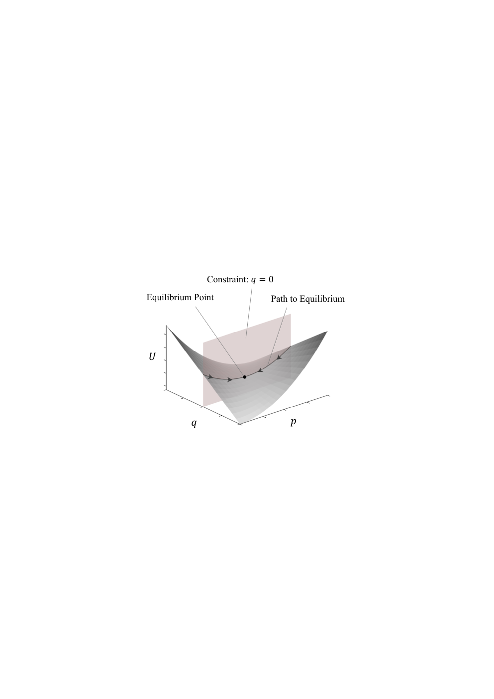
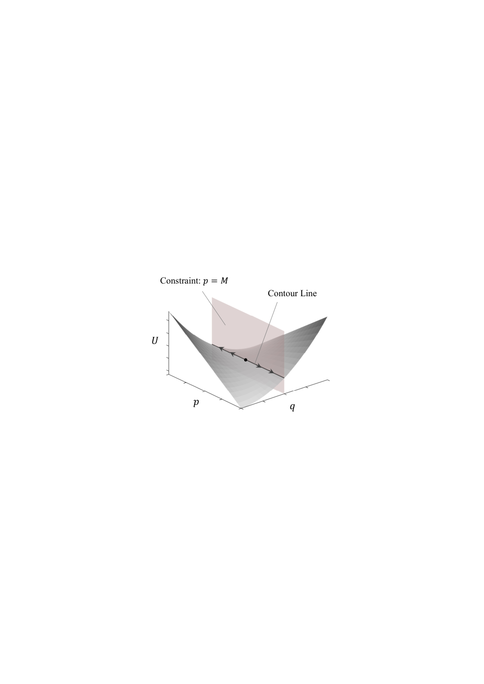
The condition in Eq. (3) means that the potential $U$ of the LA-GBM attains a local minimum $U^{*}$ on a hyperplane where the active variables $\bm{q}$ are fixed at a certain value $\bm{q}^{*}$, and that, once the passive variables $\bm{p}$ are fixed at $\bm{p}=\bm{p}^{*}$, the potential $U$ remains at the same minimum value $U^{*}$ regardless of the values of the active variables $\bm{q}$. This condition represents the load-adaptation process along a path toward the local minimum value $U^{*}$ and the gravity-balancing process along a path on which the potential remains at $U^{*}$ (Fig. 2), and is used in the derivation of the factorized form in Sec. 2.4. In contrast, the condition in Eq. (4) is introduced as a functional requirement of the LA-GBM and requires that the mechanism be capable of lifting the payload during the gravity-balancing process (Fig. 3).

As an example of an existing mechanism, the lever-arm mechanism shown in Fig. 4 is examined to confirm that it functions as a defined LA-GBM. In this mechanism, the slider is directly connected to the payload $M$, and the payload height is given by the height of the tip of the lever arm minus the slider displacement. Accordingly, the potential field generated by this mechanism is expressed as follows.

$$U(q,p;M)=Mg(l\sin{q}-p)+\frac{1}{2}k{(l^{2}+p^{2}-2lp\sin{q})}$$

(5)

Here, $g$ denotes the gravitational acceleration, $l$ denotes the length of the lever arm and the mounting height of the spring, and $k$ denotes the spring stiffness. In addition, the lever-arm angle $q$ is used as the active variable $\bm{q}$ of the mechanism, while the slider displacement $p$ is used as the passive variable $\bm{p}$. The movable domain $\Omega$ is defined as

$$\Omega=\left\{(q,p)\in\mathbb{R}^{2}\mid-\pi/2<q<\pi/2,\;0\leq p\leq l\right\},\ \ \ Mg/k<l$$

(6)

First, under the constraint condition that keeps the lever arm horizontal, $q=0$, Eq. (5) becomes

$$\frac{\partial U}{\partial p}(0,p;M)=kp-Mg$$

(7)

$$\frac{\partial^{2}U}{\partial p^{2}}(0,p;M)=k>0$$

(8)

This means that, under the constraint condition $q=0$, the passive variable $p$ moves toward the local minimum point $p=Mg/k$. Furthermore, when the passive variable $p$ is fixed at the equilibrium point $p=Mg/k$ obtained through the load-adaptive operation,

$$\frac{\partial U}{\partial q}(q,Mg/k;M)=(Mgl-klp)\cos{q}\big|_{p=Mg/k}=0$$

(9)

holds for any $q$ within the movable domain. In other words, when $p$ is fixed at $p=Mg/k$, the potential $U$ remains constant regardless of $q$. From Eqs. (7)–(9), the potential $U$ formed by this mechanism satisfies condition (3).

Furthermore, since the potential energy $U_{g}$ of the payload $M$ satisfies

$$\frac{\partial U_{g}}{\partial q}(q,Mg/k;M)=M\frac{\partial f}{\partial q}(q,Mg/k)=Mgl\cos{q}\neq 0,$$

(10)

the potential $U$ formed by this mechanism also satisfies condition (4).

In the following, the affine form and the factorized form, which represent general forms of the potential $U$ of mechanisms such as the example above, are derived in Secs. 2.3 and 2.4, respectively.

In this section, the potential field $U$ formed by an LA-GBM is generalized as an affine function with respect to the payload $M$. The generalization in affine form explicitly shows that the potential $U$ formed by an LA-GBM can be represented as the superposition of the potential energy $U_{g}$ associated with the payload $M$ and the compensating potential $U_{c}$ generated by elements such as counterweights and springs.

The affine form of the potential field generated by an LA-GBM is given by the following function.

$$U(\bm{q},\bm{p};M)=Mf(\bm{q},\bm{p})+h(\bm{q},\bm{p})$$

(11)

Here, $f(\bm{q},\bm{p})$ and $h(\bm{q},\bm{p})$ are arbitrary smooth functions of the state variables $\bm{q}$ and $\bm{p}$. Equation (11) is an extension of the law of conservation of mechanical energy under quasi-static operation, which is known as one of the most fundamental properties satisfied by GBMs [1][24],

$$U=U_{g}+U_{c}$$

(12)

with the additional consideration of the effect of the payload $M$. The derivation of Eq. (11) is presented below.

First, the potential energy $U_{g}$ of the payload can be expressed as the product of the payload $M$ and the term $f(\bm{q},\bm{p})$ corresponding to its vertical displacement, as follows.

$$U_{g}(\bm{q},\bm{p};M)=Mf(\bm{q},\bm{p}).$$

(13)

Furthermore, when the payload $M$ varies from task to task, mechanism parameters such as the spring stiffness and the counterweight mass cannot be adjusted according to the payload $M$, and all resulting changes in the mechanism state are reflected in the state variables $\bm{q}$ and $\bm{p}$. Therefore, the compensating potential $U_{c}$ of an LA-GBM without additional operations can be described as follows by a function $h=h(\bm{q},\bm{p})$ whose arguments consist only of the state variables.

$$U_{c}(\bm{q},\bm{p};M)=h(\bm{q},\bm{p}).$$

(14)

Finally, by substituting Eqs. (13) and (14) into Eq. (12), Eq. (11) is obtained as the general form of the potential field $U$ of an LA-GBM that handles an unknown payload $M$.

Furthermore, under Eq. (11), condition (4) can be expressed in terms of the function $f$ as follows.

$$\exists\bm{q}\in\pi_{\bm{q}}(\Omega),\nabla_{\bm{q}}f(\bm{q},\bm{p}^{*})\neq\bm{0}.$$

(15)

In this section, the potential field $U$ formed by an LA-GBM is generalized in a factorized form. The generalization in factorized form explicitly represents the load-adaptive operation as a state transition toward an equilibrium point of the potential field and the gravity-balancing operation as a state transition along a contour of the potential field.

The factorized form is given by the following function.

$$U(\bm{q},\bm{t};M)=\psi(\bm{t};M)+\bm{q}^{\mathrm{T}}B(\bm{q},\bm{t};M)\bm{t}.$$

(16)

Here, $\psi(\bm{t};M)\in\mathbb{R}$ and $B(\bm{q},\bm{t};M)\in\mathbb{R}^{m\times n}$ are arbitrary functions, and the variable $\bm{t}$ is an alternative representation of the passive variable $\bm{p}$ defined by the following variable transformation.

$$\exists\bm{q}^{*},\bm{t}=\frac{\partial U}{\partial\bm{p}}(\bm{q}^{*},\bm{p};M).$$

(17)

It is assumed that, in a neighborhood of $\bm{p}=\bm{p}^{*}$ satisfying $\bm{t}=\bm{0}$, the Hessian matrix $\nabla_{\bm{p}}^{2}U(\bm{q}^{*},\bm{p};M)$ is positive definite and the variable transformation is regular. The derivation of Eq. (16) is presented below.

First, the potential $U$ is expressed as the following series in the form of a polynomial in $\bm{q}$ and $\bm{t}$.

$$U(\bm{q},\bm{t};M)=\phi(\bm{q};M)+\psi(\bm{t};M)+\bm{q}^{\mathrm{T}}B(\bm{q},\bm{t};M)\bm{t}.$$

(18)

The load-adaptive operation can be interpreted as a state transition toward the equilibrium point $\partial U/\partial\bm{p}(\bm{q}^{,}\bm{p}^{;}M)=\bm{0}$ on the hyperplane where the active variable $\bm{q}$ is fixed at $\bm{q}=\bm{q}^{*}$. That is, when there exists a state $(\bm{q}^{*},\bm{p}^{*})$ satisfying $\bm{t}(\bm{q}^{*},\bm{p}^{*};M)=\bm{0}$, the potential $U(\bm{q},\bm{t};M)$ attains the local minimum value $U^{*}(M)=U(\bm{q}^{,}\bm{0};M)$. Furthermore, during the gravity-balancing operation, the state must transition along a contour on the hyperplane where the passive variable $\bm{p}$ is fixed at $\bm{p}=\bm{p}^{*}$. Therefore, the following condition must be satisfied:

$$\forall\bm{q}\in\pi_{\bm{q}}(\Omega),\ \ U(\bm{q},\bm{0};M)=U^{*}(M).$$

(19)

Substituting the condition in Eq. (19) into Eq. (18) eliminates the third term on the right-hand side, indicating that $\phi(\bm{q};M)$ is a constant function.

	$\displaystyle U(\bm{q},\bm{0};M)$	$\displaystyle=\phi(\bm{q};M)+\psi(\bm{0};M)=U^{*}(M)$		(20)
	$\displaystyle\therefore\phi(\bm{q};M)$	$\displaystyle=\phi(M).$

In this case, $\phi(M)$ can be absorbed into the function $\psi(\bm{t};M)$ by applying the mapping $\phi(M)+\psi(\bm{q};M)\mapsto\psi(\bm{q};M)$. Consequently, the factorized form in Eq. (16) is obtained.

This section describes the design flow for LA-GBMs using generative AI. In the proposed method, the affine form in Eq. (11), the factorized form in Eq. (16), and the variation in the payload potential energy expressed by Eq. (15) are provided to the generative AI as design requirements representing the general forms and conditions that the potential field of an LA-GBM must satisfy. The parameters required for the design are the dimensions $m$ and $n$ of the state variables $\bm{q}$ and $\bm{p}$, respectively.

Generative AI is used to search for candidate potential functions that satisfy these conditions, and the validity of the obtained functions is verified through the analysis described later. Therefore, in the proposed method, generative AI is positioned not as the direct designer of the LA-GBM, but as a search tool for generating design candidates from a theoretically defined function space.

This section presents an example in which candidate potential fields for an LA-GBM were generated using generative AI. For the generation of the potential field, GPT-5.6 Sol, a large language model provided by OpenAI, was used.

In this study, the model was used in a new conversation environment to minimize, as much as possible, the influence of prior conversation history and additional information specific to this study on the generated results. No fine-tuning or additional training was performed for this study. Instead, the design requirements formulated in the preceding sections were provided as input conditions, and the model was asked to generate candidate potential functions satisfying these requirements. The generation was performed on September 17, 2026 (Japan Standard Time). In addition, to obtain nontrivial solutions applicable to multi-degree-of-freedom systems, the active variable $\bm{q}$ was set as an $m$-dimensional real vector, $\bm{q}\in\mathbb{R}^{m}$, and the passive variable $\bm{p}$ as an $n$-dimensional real vector, $\bm{p}\in\mathbb{R}^{n}$.

The potential field $U$ generated by the AI is given as follows.

$$U(\bm{q},\bm{p};M)=\frac{1}{2}\bm{p}^{\rm{T}}\bm{p}+\bm{q}^{\rm{T}}A\bm{p}-M\big(\bm{b}^{\rm{T}}\bm{p}+\bm{q}^{\rm{T}}A\bm{b}).$$

(21)

Here, $A\in\mathrm{R}^{m\times n}$ and $\bm{b}\in\mathrm{R}^{n}$ are an arbitrary constant matrix and an arbitrary constant vector, respectively, satisfying $A\bm{b}\neq\bm{0}$. Figure 7 shows a schematic of the potential field in Eq. (21) for the case $\bm{q}\in\mathbb{R}$ and $\bm{p}\in\mathbb{R}$.

First, it is confirmed that Eq. (21) can be represented in both the affine form of Eq. (11) and the factorized form of Eq. (16). Equation (21) takes the affine form of Eq. (11) by defining the functions $f(\bm{q},\bm{p})$ and $h(\bm{q},\bm{p})$ as follows.

$$f(\bm{q},\bm{p})=-\big(\bm{b}^{\rm{T}}\bm{p}+\bm{q}^{\rm{T}}A\bm{b}),$$

(22)

$$h(\bm{q},\bm{p})=\frac{1}{2}\bm{p}^{\rm{T}}\bm{p}+\bm{q}^{\rm{T}}A\bm{p}.$$

(23)

Furthermore, when $\bm{t}\in\mathbb{R}^{n}$ is defined in the state $\bm{q}=\bm{0}$ as

	$\displaystyle\bm{t}$	$\displaystyle=\nabla_{\bm{p}}U(\bm{0},\bm{p};M)=\bm{p}-M\bm{b}$		(24)
	$\displaystyle\therefore\bm{p}$	$\displaystyle=\bm{t}+M\bm{b}$

substituting Eq. (24) into Eq. (21) yields the following expression.

$$U(\bm{q},\bm{t};M)=\frac{1}{2}\big(\bm{t}^{\rm{T}}\bm{t}-M^{2}\bm{b}^{\rm{T}}\bm{b}\big)+\bm{q}^{\rm{T}}A\bm{t}.$$

(25)

Equation (25) coincides with the factorized form expressed by Eq. (16) by defining $\psi(\bm{t};M)$ and $B(\bm{q},\bm{t};M)$ as

$$\psi(\bm{t};M)=\frac{1}{2}\big(\bm{t}^{\rm{T}}\bm{t}-M^{2}\bm{b}^{\rm{T}}\bm{b}\big),$$

(26)

$$B(\bm{q},\bm{t};M)=A.$$

(27)

It can also be confirmed that, when $\bm{t}=\nabla_{\bm{p}}U(\bm{0},\bm{p};M)=\bm{0}$, Eq. (25) becomes

$$U(\bm{q},\bm{0};M)=-\frac{1}{2}M^{2}\bm{b}^{\rm{T}}\bm{b}=\rm{const}.$$

(28)

and therefore directly satisfies the condition in Eq. (3).

Furthermore, calculating the gradient $\nabla_{\bm{q}}f$ of Eq. (22) with respect to the active variable $\bm{q}$ gives

$$\nabla_{\bm{q}}f=-A\bm{b}\neq\bm{0}.$$

(29)

which also satisfies the requirement for variation in the payload potential energy expressed by Eq. (15).

From the above results, it can be concluded that the function search using AI successfully generated a potential field satisfying the requirements of an LA-GBM.

This section describes the process of constructing a gravity-balancing mechanism based on the potential field $U$ obtained in Sec. 3.2. For simplicity, the dimensions of both the active variable $\bm{q}$ and the passive variable $\bm{p}$ are set to $1$, and they are denoted as the scalar quantities $\bm{q}=q$ and $\bm{p}=p$ for convenience. Accordingly, the dimension of the variable $\bm{t}$ is also $1$, and it is denoted as $\bm{t}=t$. For further simplification, $A=1$ and $b=1$ are assumed. Under these assumptions, Eq. (21) is simplified as follows.

$$U(q,p;M)=\frac{1}{2}p^{2}+qp-M(q+p).$$

(30)

If the potential fields corresponding to the individual terms in Eq. (30) can be reproduced using existing mechanical elements, an LA-GBM can be designed based on the function generated by AI. In the following discussion, all terms in Eq. (30) are assumed to have been converted to the dimension of energy using appropriate physical constants or conversion coefficients.

The potential field in Eq. (30) can be reproduced by combining a linear spring, a counterweight, and a linkage mechanism that outputs the product of two displacement inputs. First, the first term on the right-hand side of Eq. (30) is a quadratic function of $p$ and can therefore be reproduced using a spring whose elongation is proportional to the state $p$. Next, the second term on the right-hand side can be reproduced by constructing a linkage mechanism that generates a vertical displacement equal to the product $qp$ and attaching a counterweight to it. Several linkage mechanisms that output the product of state variables have previously been proposed [38, 39, 40]. Finally, the third term on the right-hand side can be reproduced by constructing a linkage mechanism that generates a vertical displacement equal to the sum $q+p$ and attaching the payload $M$ to it. By constructing a mechanism in which these three elements are connected in parallel, the potential field in Eq. (30) can be reproduced (Fig. 8).

Since the primary objective of this paper is to present a new design method for LA-GBMs, fabrication and experimental validation of the design result represented by Eq. (30) are left for future work.

References

- [1] Nguyen, V. L., 2026, “Passive Gravity Compensation in Mechanisms and Robots: Methods, Advances, and Challenges,” Mechanism and Machine Theory, 220, 106345, doi: 10.1016/j.mechmachtheory.2025.106345.
- [2] Lu, Q., Ortega, C., and Ma, O., 2011, “Passive Gravity Compensation Mechanisms: Technologies and Applications,” Recent Patents on Engineering, 5(1), pp. 32–44, doi: 10.2174/1872212111105010032.
- [3] Chheta, Y. R., Joshi, R. M., Gotewal, K. K., and ManoahStephen, M., 2017, “A Review on Passive Gravity Compensation,” Proceedings of the 2017 International Conference of Electronics, Communication and Aerospace Technology (ICECA), Coimbatore, India, pp. 184–189, doi: 10.1109/ICECA.2017.8203668.
- [4] Bruzzone, L., and Bozzini, G., 2011, “A Statically Balanced SCARA-Like Industrial Manipulator With High Energetic Efficiency,” Meccanica, 46(4), pp. 771–784, doi: 10.1007/s11012-010-9336-6.
- [5] Arakelian, V., 2016, “Gravity Compensation in Robotics,” Advanced Robotics, 30(2), pp. 79–96, doi: 10.1080/01691864.2015.1090334.
- [6] Parekh, P. P., Gotewal, K. K., Manoah, M. S., and Bhavsar, K., 2020, “Review on Gravity Compensation by Mechanism Synthesis,” Manufacturing Technology Today, 19(1–2), pp. 53–60.
- [7] Park, K.-S., and Lee, K.-M., 2026, “A Review of Passive Linear Gravity Compensation Mechanisms,” Actuators, 15(2), 111, doi: 10.3390/act15020111.
- [8] Tojo, Y., Debenest, P., Fukushima, E. F., and Hirose, S., 2004, “Robotic System for Humanitarian Demining: Development of Weight-Compensated Pantograph Manipulator,” Proceedings of the 2004 IEEE International Conference on Robotics and Automation (ICRA), New Orleans, LA, USA, pp. 2025–2030.
- [9] Whitney, J. P., and Hodgins, J. K., 2014, “A Passively Safe and Gravity-Counterbalanced Anthropomorphic Robot Arm,” Proceedings of the 2014 IEEE International Conference on Robotics and Automation (ICRA), Hong Kong, China, pp. 6168–6173, doi: 10.1109/ICRA.2014.6907768.
- [10] Kayawake, R., Abe, K., Watanabe, M., Tadakuma, K., and Tadokoro, S., 2024, “Gravity Compensation Mechanism Inspired by Sauropods’ Skeleton,” Proceedings of the 2024 IEEE/ASME International Conference on Advanced Intelligent Mechatronics (AIM), Boston, MA, USA, pp. 1272–1277, doi: 10.1109/AIM55361.2024.10637138.
- [11] French, M. J., and Widden, M. B., 2000, “The Spring-and-Lever Balancing Mechanism, George Carwardine and the Anglepoise Lamp,” Proceedings of the Institution of Mechanical Engineers, Part C: Journal of Mechanical Engineering Science, 214(3), pp. 501–508, doi: 10.1243/0954406001523137.
- [12] Endo, G., Yamada, H., Yajima, A., Ogata, M., and Hirose, S., 2010, “A Passive Weight Compensation Mechanism With a Non-Circular Pulley and a Spring,” Proceedings of the 2010 IEEE International Conference on Robotics and Automation (ICRA), Anchorage, AK, USA, pp. 3843–3848, doi: 10.1109/ROBOT.2010.5509797.
- [13] Kim, H.-S., Min, J.-K., and Song, J.-B., 2016, “Multiple-Degree-of-Freedom Counterbalance Robot Arm Based on Slider-Crank Mechanism and Bevel Gear Units,” IEEE Transactions on Robotics, 32(1), pp. 230–235, doi: 10.1109/TRO.2015.2501746.
- [14] Shi, K., Yang, J., Tong, Y., Hou, Z., and Yu, H., 2023, “Design and Analysis of a Cable-Driven Gravity Compensation Mechanism for Spatial Multi-DoF Robotic Systems,” Mechanism and Machine Theory, 190, 105452, doi: 10.1016/j.mechmachtheory.2023.105452.
- [15] Ulrich, N., and Kumar, V., 1991, “Passive Mechanical Gravity Compensation for Robot Manipulators,” Proceedings of the 1991 IEEE International Conference on Robotics and Automation (ICRA), Sacramento, CA, USA, pp. 1536–1541, doi: 10.1109/ROBOT.1991.131834.
- [16] Simionescu, I., and Ciupitu, L., 2000, “The Static Balancing of the Industrial Robot Arms: Part II: Continuous Balancing,” Mechanism and Machine Theory, 35(9), pp. 1299–1311, doi: 10.1016/S0094-114X(99)00068-3.
- [17] Takeichi, M., Suzumori, K., Endo, G., and Nabae, H., 2017, “Development of Giacometti Arm With Balloon Body,” IEEE Robotics and Automation Letters, 2(2), pp. 951–957, doi: 10.1109/LRA.2017.2655111.
- [18] Takesue, N., Komoda, Y., Murayama, H., Fujiwara, K., and Fujimoto, H., 2016, “Scissor Lift With Real-Time Self-Adjustment Ability Based on Variable Gravity Compensation Mechanism,” Advanced Robotics, 30(15), pp. 1014–1026, doi: 10.1080/01691864.2016.1181008.
- [19] Yang, Z.-W., and Lan, C.-C., 2015, “An Adjustable Gravity-Balancing Mechanism Using Planar Extension and Compression Springs,” Mechanism and Machine Theory, 92, pp. 314–329, doi: 10.1016/j.mechmachtheory.2015.05.006.
- [20] Barajas, J. C., and Paz, R. A., 2016, “Autobalancing a Generalized Gravity Equilibrator,” International Journal of Dynamics and Control, 4, pp. 515–526, doi: 10.1007/s40435-015-0173-2.
- [21] Kim, J., Moon, J., Kim, J., and Lee, G., 2020, “Compact Variable Gravity Compensation Mechanism With a Geometrically Optimized Lever for Maximizing Variable Ratio of Torque Generation,” IEEE/ASME Transactions on Mechatronics, 25(4), pp. 2019–2026, doi: 10.1109/TMECH.2020.2998291.
- [22] Kim, J., Moon, J., Ryu, J., Kim, S., Yoon, J., and Lee, G., 2022, “A Novel Energy-Efficient Actuator Integrated With Compact Variable Gravity Compensation Module,” Mechanism and Machine Theory, 177, 105031, doi: 10.1016/j.mechmachtheory.2022.105031.
- [23] Furnémont, R., Verstraten, T., Lefeber, D., and Vanderborght, B., 2022, “Prismatic Gravity Compensator for Variable Payloads,” IEEE Robotics and Automation Letters, 7(2), pp. 3749–3756, doi: 10.1109/LRA.2022.3147239.
- [24] Chew, D. X. H., Wood, K. L., and Tan, U. X., 2019, “Design of a Passive Self-Regulating Gravity Compensator for Variable Payloads,” Journal of Mechanical Design, 141(10), 102302, doi: 10.1115/1.4043582.
- [25] Wisse, B. M., van Dorsser, W. D., Barents, R., and Herder, J. L., 2007, “Energy-Free Adjustment of Gravity Equilibrators Using the Virtual Spring Concept,” Proceedings of the 2007 IEEE 10th International Conference on Rehabilitation Robotics (ICORR), Noordwijk, The Netherlands, pp. 742–750, doi: 10.1109/ICORR.2007.4428508.
- [26] Franchetti, D., Boschetti, G., and Lenzo, B., 2021, “Passive Gravity Balancing With a Self-Regulating Mechanism for Variable Payload,” Machines, 9(8), 145, doi: 10.3390/machines9080145.
- [27] van Dorsser, W. D., Barents, R., Wisse, B. M., and Herder, J. L., 2007, “Gravity-Balanced Arm Support With Energy-Free Adjustment,” Journal of Medical Devices, 1(2), pp. 151–158, doi: 10.1115/1.2736400.
- [28] Nathan, R. H., 1985, “A Constant Force Generation Mechanism,” Journal of Mechanisms, Transmissions, and Automation in Design, 107(4), pp. 508–512, doi: 10.1115/1.3260755.
- [29] Chu, Y.-L., and Kuo, C.-H., 2017, “A Single-Degree-of-Freedom Self-Regulated Gravity Balancer for Adjustable Payload,” Journal of Mechanisms and Robotics, 9(2), 021006, doi: 10.1115/1.4035561.
- [30] Barents, R., Schenk, M., van Dorsser, W. D., Wisse, B. M., and Herder, J. L., 2011, “Spring-to-Spring Balancing as Energy-Free Adjustment Method in Gravity Equilibrators,” Journal of Mechanical Design, 133(6), 061010, doi: 10.1115/1.4004101.
- [31] Nguyen, V. L., 2022, “Design of a Compact Gear-Spring Mechanism for Static Balancing of Variable Payloads,” Journal of Mechanical Design, 144(12), 123301, doi: 10.1115/1.4055121.
- [32] Lee, Y.-Y., and Chen, D.-Z., 2014, “Determination of Spring Installation Configuration on Statically Balanced Planar Articulated Manipulators,” Mechanism and Machine Theory, 74, pp. 319–336, doi: 10.1016/j.mechmachtheory.2013.12.019.
- [33] Lin, P.-Y., Shieh, W.-B., and Chen, D.-Z., 2012, “Design of Statically Balanced Planar Articulated Manipulators With Spring Suspension,” IEEE Transactions on Robotics, 28(1), pp. 12–21, doi: 10.1109/TRO.2011.2169633.
- [34] Lin, P.-Y., Shieh, W.-B., and Chen, D.-Z., 2010, “A Stiffness Matrix Approach for the Design of Statically Balanced Planar Articulated Manipulators,” Mechanism and Machine Theory, 45(12), pp. 1877–1891, doi: 10.1016/j.mechmachtheory.2010.08.003.
- [35] Nguyen, V. L., 2022, “A Design Approach for Gravity Compensators Using Planar Four-Bar Mechanisms and a Linear Spring,” Mechanism and Machine Theory, 172, 104770, doi: 10.1016/j.mechmachtheory.2022.104770.
- [36] Martini, A., Troncossi, M., and Rivola, A., 2019, “Algorithm for the Static Balancing of Serial and Parallel Mechanisms Combining Counterweights and Springs: Generation, Assessment and Ranking of Effective Design Variants,” Mechanism and Machine Theory, 137, pp. 336–354, doi: 10.1016/j.mechmachtheory.2019.03.031.
- [37] Chiang, W.-H., and Chen, D.-Z., 2017, “Design of Planar Variable-Payload Balanced Articulated Manipulators With Actuated Linear Ground-Adjacent Adjustment,” Mechanism and Machine Theory, 109, pp. 296–312, doi: 10.1016/j.mechmachtheory.2016.12.001.
- [38] Silverberg, T. R., 1959, “Precision Linkage for Exact Multiplication,” U.S. Patent No. 2,910,227.
- [39] Svoboda, A., 1950, “Multiplying Linkage,” U.S. Patent No. 2,498,310.
- [40] Brown, W. C., 1955, “Mechanical Multiplier,” U.S. Patent No. 2,716,521.
- [41] Svoboda, A., 1948, Computing Mechanisms and Linkages, James, H. M., ed., Massachusetts Institute of Technology Radiation Laboratory Series, Vol. 27, McGraw-Hill, New York.
- [42] Lee, W.-T., and Russell, K., 2018, “Developments in Quantitative Dimensional Synthesis (1970–Present): Four-Bar Path and Function Generation,” Inverse Problems in Science and Engineering, 26(9), pp. 1280–1304, doi: 10.1080/17415977.2017.1396328.