Bridging Body and Brain:
Gene-Driven Morphology–Control Co-Design
Abstract
Morphology–control co-design jointly optimizes an agent’s body structure and control policy as an integrated embodied system. However, existing methods typically model morphology design and control with separate networks coupled only indirectly through a shared task objective, limiting explicit high-level coordination. Inspired by natural genes that coordinate biological development, we introduce Morphogene, a compact latent blueprint that bridges an agent’s body and brain. Through AdaConcat, Morphogene jointly conditions morphology and control generation at the limb level, allowing its variations to induce coordinated changes in both components. Building on this representation, we propose GeCode, which formulates co-design as exploration in the compact Morphogene space. Each Morphogene anchors a local design region in which nearby body–brain designs are explored, while performance-guided updates move these anchors toward promising regions for more efficient exploration of the broader design space. This process combines local refinement with global exploration while preserving body–brain compatibility. Extensive experiments across diverse 2D and 3D co-design tasks demonstrate that GeCode consistently outperforms existing state-of-the-art methods, achieving substantially faster convergence and higher final performance.

1 Introduction
Across species in nature, body morphology and neural control develop and evolve together, with the body shaping the physical conditions for behavior and the nervous system adapting to exploit them (Chiel and Beer, 1997; Bartolozzi et al., 2022). Nevertheless, embodied-agent design often treats morphology and control as largely independent components (Xiong et al., 2023; Gupta et al., 2021). Such one-sided optimization either confines control to the affordances of a fixed body (Haarnoja et al., 2024; Bolotnikova et al., 2025) or yields morphologies biased toward a fixed controller (Matthews et al., 2023; Zhao et al., 2020), motivating morphology–control co-design through the joint adaptation of agent’s body and brain (Ha, 2019; Liu et al., 2025; Wang et al., 2025).
However, current embodied co-design methods typically employ separate morphology-generation and control-policy networks coupled primarily through the shared task objective (Eq. (1)) rather than explicit coordination at the representation or decision level (Yuan et al., 2022; Lu et al., 2025). Consequently, morphological changes do not directly guide controller adaptation, nor do controller updates explicitly inform morphological design; this weak coupling obscures cross-component credit assignment and leaves body–brain coordination indirect and inadequately modeled (Dai et al., 2026).
In nature, genes address an analogous coordination problem by serving as developmental blueprints that encode shared high-level programs. Variations in these programs jointly shape morphology, neural circuitry, and behavior beyond adaptation driven solely by environmental feedback (Zador, 2019; Fleck et al., 2023). Inspired by this principle, we introduce Morphogene as a similar developmental blueprint for embodied agents. Rather than representing a single fixed morphology, each Morphogene abstracts high-level structural and geometric characteristics, anchors a local region of related body designs, and jointly conditions morphology generation and controller adaptation11 1 The anchoring role of a Morphogene resembles that of a prototype in representation learning. Here, however, we use the biologically inspired term developmental blueprint to emphasize its broader role: beyond serving as a representative embedding, a Morphogene can be adaptively moved through the latent space to guide morphology design while bridging morphology generation and controller adaptation in embodied agents..
Specifically, unlike conventional approaches that model body and brain with separate networks (Yuan et al., 2022; Lu et al., 2025), a shared Morphogene explicitly couples morphology and control generation at the representation level. Morphogene is injected into both networks through AdaConcat, which transforms the agent-level representation into limb-specific conditions based on each limb’s structural and functional role. Consequently, variations in Morphogene induce coherent changes in morphology design and corresponding controller adaptations, thereby bridging body and brain.
Building on Morphogene, we introduce GeCode, a gene-driven co-design framework that shifts co-design from a discrete morphology-design space (Gupta et al., 2021; Koike et al., 2024) to a compact, continuous Morphogene space. Specifically, GeCode maintains a small set of Morphogenes as design anchors, combining stochastic policy rollouts with a Morphogene-proximity reward to explore high-performing, locally coherent body–brain designs around each anchor. Performance-guided Morphogene updates subsequently move the anchors toward regions of higher-performing body–brain designs, thereby expanding exploration across the latent space. This local-to-global strategy enables broad yet targeted exploration without exhaustively evaluating discrete morphologies.
We evaluate GeCode across twelve 2D and 3D design spaces spanning diverse morphologies. GeCode consistently outperforms state-of-the-art methods, achieving on average 2.5 faster convergence and 69.48% higher task performance while incurring less than 4.0% additional wall-clock overhead.
Our contributions are as follows: (1) We introduce Morphogene, a high-level latent blueprint that bridges an agent’s body and brain, together with AdaConcat for adaptive, limb-aware conditioning of morphology and control. (2) We propose GeCode, which reformulates morphology–control co-design as gene-driven exploration in the compact Morphogene space, allowing latent updates to induce coordinated body–brain adaptation. (3) Extensive experiments demonstrate that GeCode achieves state-of-the-art performance with faster convergence and higher final returns.
2 Related Work
Morphology–Control Co-design
Joint morphology–control optimization has emerged as a promising direction in embodied intelligence (Strgar and Kriegman, 2026; Fay et al., 2026; Wang et al., 2025; Liu et al., 2025). Early evolutionary approaches relied on population-based morphology search and repeated controller adaptation, resulting in substantial sampling and computational costs (Bhatia et al., 2021; Gupta et al., 2021; Cheney et al., 2018). Recent RL-based methods jointly optimize sequential morphology construction and control (Yuan et al., 2022; Wang et al., 2023; Lu et al., 2025). However, their separate morphology and control networks remain weakly coupled, limiting explicit body–brain coordination. StackelbergPPO (Dai et al., 2026) strengthens optimization-level coordination by explicitly modeling morphology–control interdependence, but still leave their representation-level coupling implicit. In contrast, GeCode makes this coupling explicit through Morphogene, which jointly coordinates morphology and control generation throughout co-design.
Further discussion on “Genes” in Intelligent Agents and Universal Control is provided in App. A.
3 Preliminaries
Morphology Representation
An agent’s morphology is represented as an undirected graph , where each node denotes a limb and each edge denotes a joint connecting two limbs. The attribute set specifies limb properties (e.g., length and size) and joint properties (e.g., rotation ranges and motor torques).
Once the topology and attributes are specified, the simulator (MuJoCo in our implementation) instantiates the morphology. In our design spaces, each limb is paired with exactly one associated joint, denoted by , allowing their simulator-derived attributes to be combined as . Here, encodes fixed limb geometry, such as its reference position and orientation (e.g., body_pos and body_iquat), while encodes the corresponding joint geometry (e.g., jnt_pos). The complete vector representation is . Thus, and describe the same morphology at the graph and vector levels, respectively, with the former used for sequential morphology design and the latter for constructing the Morphogene space.
Morphology-Control Co-Design Optimization
Morphology–control co-design optimizes an agent’s body structure and control policy through a Design Stage and a Control Stage . During morphology design , the morphology graph is sequentially updated over topology design steps followed by attribute design steps. Each update follows
where . is the morphology-design policy, and is the corresponding transition function. The morphology-editing action specifies structural operations (e.g., adding or removing limbs) during topology design and physical-attribute updates (e.g., adjusting limb length) during attribute design. The resulting action sequence yields the final morphology .
During the control stage , the morphology remains fixed while the controller interacts with the environment to maximize the expected task return. At each control step, the interaction follows
Here, denotes the environment observation received by the controller, while and denote the control policy and environment transition function under , respectively.
The morphology–control co-design objective jointly optimizes the design and control policy parameters to maximize the expected discounted return:
| (1) |
Here, is the discount factor, and denotes the task reward provided by the environment (App. B).
Existing methods (Lu et al., 2025; Yuan et al., 2022) use separate morphology and control policies coupled mainly through the shared objective in Eq. (1), leaving no explicit mechanism to coordinate morphological changes with controller adaptation. To explicitly couple these two components, we formulate morphology generation and controller adaptation as Morphogene-conditioned processes (Sec. 4.2) and jointly optimize them under the augmented objective in Eq. (11).
Transformer-based Morphology Design and Control
An agent is represented by an ordered sequence of limb-wise states, where is the proprioceptive observation of limb . Each state is projected into an embedding space, and the resulting limb tokens are assembled as
| (2) |
where is the shared embedding function (Gupta et al., 2022).
The Transformer encoder comprises pre-normalized blocks, each applying layer normalization (LN) (Xiong et al., 2020) before multi-head self-attention (MSA) (Vaswani et al., 2017) and a feed-forward network (FFN), followed by residual updates:
| (3) |
The final token representation is mapped by a linear action head to the distribution parameters . During the design stage , discrete actions follow a categorical distribution parameterized by . During the control stage , continuous actions follow a Gaussian distribution , whose mean and covariance are parameterized by .
4 Method
4.1 Morphogene: A Latent Blueprint for Body–Brain Coordination
Morphology Encoding and Morphogene Representation
We define Morphogene as a compact latent blueprint that guides morphology generation and compatible control. To ground this blueprint in the underlying body structure, we learn a latent space that captures the correlated structural and geometric factors of morphology. As illustrated in Figure 2(a), the morphology encoder maps an instantiated morphology to its morphology code :
| (4) |
Unlike morphology code , which encodes a specific realized morphology, a Morphogene serves as a searchable anchor in the same latent space. GeCode then iteratively updates these anchors to drive exploration of coordinated body–brain designs (Sec. 4.3).
RAE-based Morphogene Space Construction
The Morphogene space is learned using a regularized autoencoder (RAE), whose decoder reconstructs morphological attributes and predicts limb presence, thereby preserving structural and geometric information:
| (5) |
Here, denotes the predicted limb-presence mask, which determines the number of limbs in the reconstructed morphology. The RAE is trained using a masked, regularized reconstruction objective:
| (6) |
where measures reconstruction error over valid morphology components, supervises limb-presence prediction, and regularizes the morphology codes to promote a compact Morphogene space.
Structural Constraints on the Morphogene Space
While the reconstruction objective preserves the information required for morphology recovery, it does not explicitly impose meaningful geometric structure on the Morphogene space. We therefore regularize RAE with a topology-aware contrastive loss (Eq. (18)) and a tree-structured metric loss (Eq. (19)), detailed in App. C.2.
Specifically, clusters morphology codes with identical topologies while separating those with different topologies, whereas enforces relative-distance margins between structurally similar and dissimilar morphologies. Together, these losses align latent geometry with morphological relationships, thereby enabling smooth Morphogene exploration, as visualized in Figure 6(b).
4.2 Morphogene-Conditioned Morphology Design and Control
GeCode jointly conditions the morphology-design policy and control policy on a shared Morphogene , initially sampled at random from the learned Morphogene space, thereby explicitly coupling body and brain. Following Eq. (2), the state of limb is first mapped to a stage-specific feature , where denotes the active stage.
AdaConcat for Limb-wise Condition Injection
As the agent-level Morphogene captures the morphology as a whole, uniformly injecting it across limbs cannot reflect their distinct structural and functional roles. We therefore introduce AdaConcat to adapt for limb-specific conditioning:
| (7) |
where is the positional embedding of limb , and is the modulation network. For limb , AdaConcat transforms into the corresponding limb-specific condition as
| (8) |
where denotes element-wise multiplication. See Figure 2(b) for an illustration.
The limb-specific condition is concatenated with its corresponding limb feature to form the conditioned token . The conditioned tokens are assembled as and processed by the Transformer blocks in Eq. (3), yielding a morphology-editing action during or a control action during :
| (9) |
In this way, the shared Morphogene aligns morphology generation with controller adaptation, allowing its variations to induce coherent body–brain changes for explicit morphology–control co-design.

Morphogene-Guided Local Exploration
During co-design, each Morphogene anchors a local design region for exploring nearby high-performing morphology variants. GeCode promotes such exploration by augmenting the task objective in Eq. (1) with a Morphogene-proximity reward:
| (10) |
At the end of , the generated morphology is mapped to its morphology code using Eq. (4). A reward of is assigned when the cosine similarity between the morphology code and its corresponding Morphogene exceeds . Thus, the joint training objective is
| (11) |
Consequently, the morphology-design policy is optimized to maximize task return within the -neighborhood of its conditioning Morphogene. This local search yields high-performing candidates for Morphogene updates, which subsequently drive global exploration of the latent space.
4.3 GeCode: Morphogene-Driven Co-design Optimization
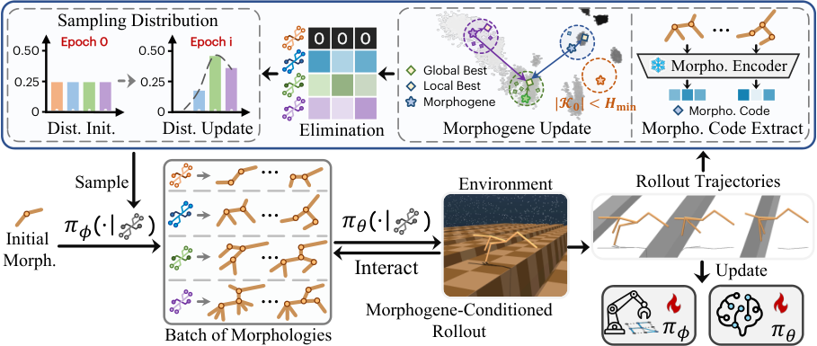
GeCode performs morphology–control co-design in the compact Morphogene space, where each Morphogene serves as a design anchor for body–brain coordination (Figure 3; Algorithm 1). These anchors are updated using existing rollout statistics to efficiently explore diverse body–brain designs, requiring neither additional environment interactions nor gradient-based latent optimization.
Morphogene Initialization
GeCode initializes a small set of Morphogenes, , by randomly and independently sampling from the learned RAE latent distribution. These Morphogenes are then iteratively refined throughout co-design, with no new Morphogenes introduced thereafter.
Morphogene-Conditioned Rollout
At each co-design epoch, each rollout first samples a Morphogene according to , where is the performance-adaptive sampling distribution. It is initialized only once at epoch with and iteratively updated after every subsequent epoch according to Eq. (14). The sampled remains fixed throughout the rollout and conditions both the morphology-design and control policies through AdaConcat (Figure 2(b)).
Because the morphology-design actions in Eq. (9) are sampled stochastically, rollouts conditioned on the same may produce distinct morphology variants within the local design region anchored by , thereby enabling local exploration around the anchor.
Morphogene Update
After each epoch’s rollouts, GeCode updates each Morphogene using the morphology codes of the best-performing design within its local region and across the entire set, referred to as the local and global best, respectively. The former preserves anchor-specific morphological characteristics, whereas the latter propagates the best-performing body–brain design across Morphogenes, thereby driving global exploration of the latent design space (see Figure 6(b)).
Specifically, each morphology generated by rollout conditioned on Morphogene is mapped to its morphology code according to Eq. (4). To preserve locality around , we retain the rollout indices , where filters out morphology codes that deviate excessively from their conditioning Morphogenes. The retained rollouts across all Morphogenes are collected in .
Let and denote the codes of the morphologies produced by the highest-return rollouts in and , with corresponding returns and , respectively. Their weighted combination defines the update target for :
| (12) |
Here, adaptively balances global guidance across Morphogenes, while controls the Morphogene update rate.
Morphogene Elimination
At the end of each epoch, a Morphogene is retained only if at least of its conditioned rollouts generate morphologies within its local region. Accordingly, the active Morphogene set is updated as
| (13) |
This procedure progressively eliminates Morphogenes that cannot be reliably realized by the morphology-design policy until only one remains.
Adaptive Morphogene Sampling
After eliminating Morphogenes, GeCode sets their next-epoch sampling probabilities using the mean return of the top- rollouts for each retained :
| (14) |
Here, denotes the return of rollout conditioned on , with .
Overall, GeCode coordinates global exploration through Morphogene updates with local exploration through stochastic Morphogene-conditioned rollouts. By operating on low-dimensional Morphogenes and reusing policy-training rollouts, it requires only lightweight vector operations, enabling efficient Morphogene-driven morphology–control co-design.
5 Experiments
Our experiments evaluate whether Morphogene effectively bridges an agent’s body and brain and whether GeCode leverages this coordination to achieve sample-efficient, high-performing morphology–control co-design. We further analyze the mechanisms underlying these gains.
Environments
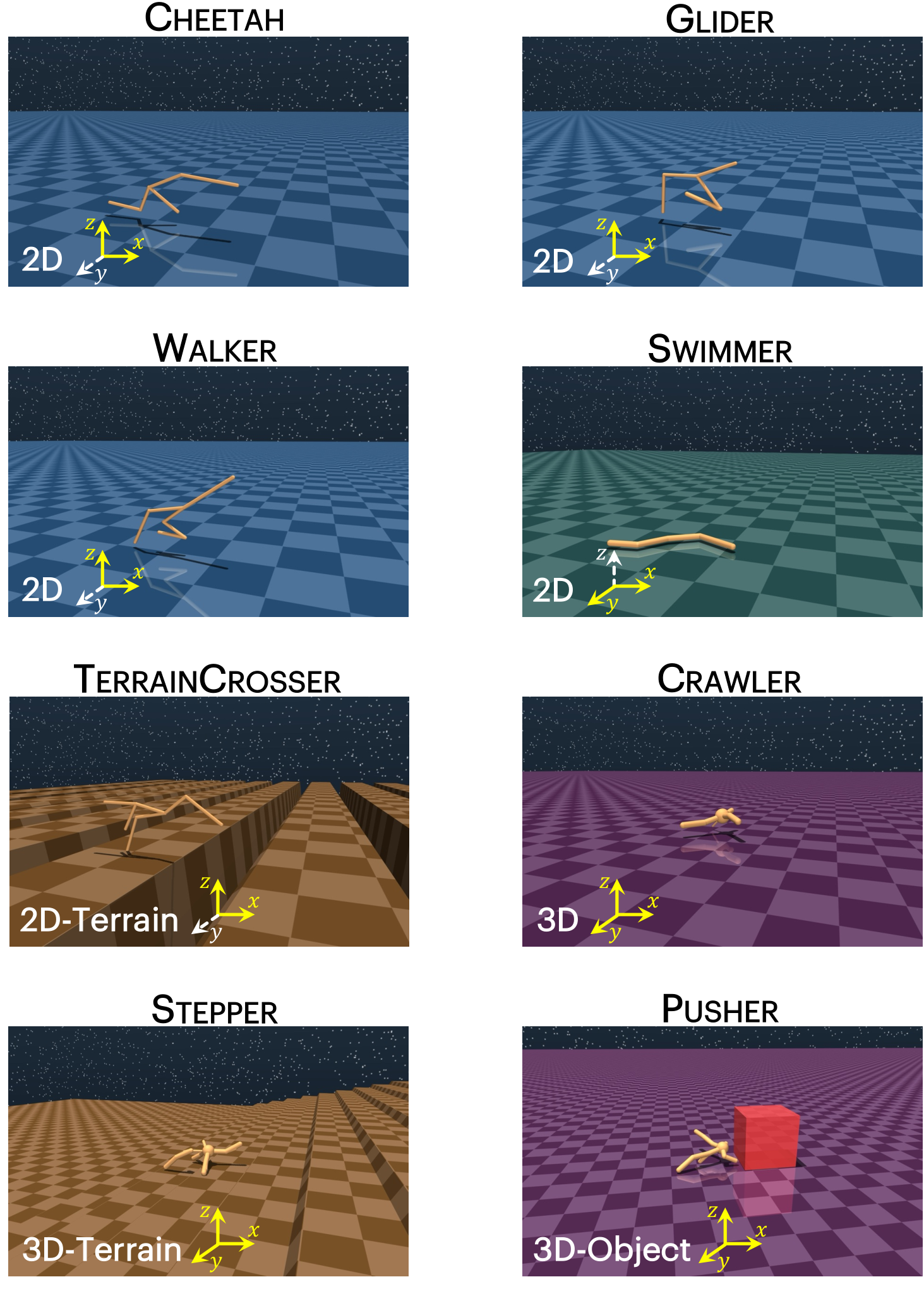
Following prior work (Lu et al., 2025; Dai et al., 2026), we evaluate GeCode across twelve MuJoCo environments (Todorov et al., 2012): Crawler, Stepper, Pusher, TerrainCrosser, Cheetah, Swimmer, Glider-(Regular, Medium, Hard) and Walker-(Regular, Medium, Hard). These 2D and 3D benchmarks cover locomotion and manipulation across diverse design spaces and terrains. Further details are provided in App. B.
5.1 Comparison with Baselines
Baselines
We build GeCode on (1) BodyGen (Lu et al., 2025), a PPO-based Transformer framework for morphology–control co-design. GeCode augments this backbone with Morphogenes that bridge body generation and controller adaptation, while Morphogene updates drive efficient exploration of coordinated body–brain designs. BodyGen therefore serves as a direct baseline. We further compare GeCode with (2) StackelbergPPO (Dai et al., 2026), which formulates co-design as a Stackelberg game to explicitly model the optimization interdependence between morphology and control, and (3) Transform2Act (Yuan et al., 2022), which trains separate GNN-based policies within a unified PPO framework. Additional comparisons with evolutionary approaches such as (4) NGE (Wang et al., 2019) are reported in Table 3 of App. E.1. Implementation details are provided in App. D.
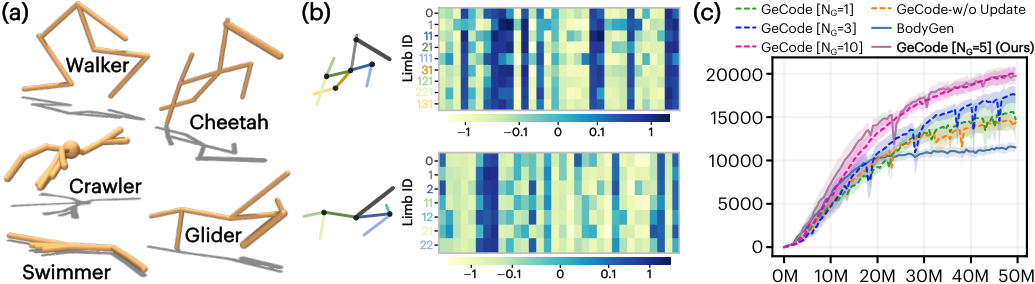
As shown in Figure 4, GeCode consistently outperforms all baselines by substantial margins, achieving an average final return approximately 69.48% higher than that of StackelbergPPO, a state-of-the-art co-design method. These gains extend beyond relatively simple tasks, such as Glider-Regular and Walker-Regular, and become more pronounced in tasks with larger morphology spaces, including Crawler, Glider-Hard, and Walker-Hard. This trend highlights how GeCode leverages Morphogene-guided exploration in a compact latent space to reduce effective search complexity as the morphology space expands. Performance gains on complex-terrain tasks such as Stepper and TerrainCrosser further highlight Morphogene’s role as a body–brain bridge, integrating proprioception with morphology-dependent contact dynamics to improve control adaptation. Representative morphologies designed by GeCode are shown in Figure 5(a).
5.2 Ablation and Analysis
In this section, we investigate five questions: (1) how Morphogene contributes separately to morphology design and control; (2) how its conditioning mechanism contributes to these benefits; (3) how Morphogene update and set size affect co-design; (4) whether structural regularization of the RAE latent space is necessary; and (5) what computational overhead the resulting procedure incurs.
Ablation of Morphogene Conditioning on Body and Brain
Morphogene bridges body and brain by jointly conditioning morphology generation and controller adaptation. To isolate its role in each component, we remove Morphogene conditioning from either the morphology-design network (w/o Gene2Body) or the control network (w/o Gene2Brain). Figure 4 shows that both ablations consistently degrade performance, confirming their complementary contributions. Specifically, conditioning morphology generation on Morphogene is particularly important in morphology-intensive tasks with large, coupled design spaces, such as Crawler and Stepper, where discovering a viable body is prerequisite to effective control. In simpler tasks with lower morphological complexity, such as Cheetah and Walker-Regular, conditioning the controller becomes more influential by enabling morphology-aware action adaptation.
| Crawler | Stepper | Pusher | Cheetah | TerrainCrosser | Swimmer | |
| w/ Direct Concat | 14049.3533.4 | 3296.0560.1 | 4289.5989.3 | 18734.4523.1 | 7826.2798.0 | 1353.527.4 |
| w/ AdaConcat | 16143.3583.0 | 3688.6271.0 | 6250.2757.9 | 19888.7944.6 | 9670.61176.4 | 1422.529.5 |
| Glider-Regular | Glider-Medium | Glider-Hard | Walker-Regular | Walker-Medium | Walker-Hard | |
| w/ Direct Concat | 20998.11002.0 | 20333.9884.1 | 18031.01571.1 | 19197.02119.3 | 19949.6856.5 | 20647.6851.3 |
| w/ AdaConcat | 23317.5627.9 | 22376.4809.9 | 19972.8332.1 | 24306.11293.0 | 21973.3918.9 | 21614.6521.8 |
Ablation on AdaConcat
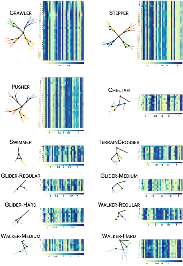
We evaluate the effectiveness of AdaConcat’s adaptive conditioning for Morphogene injection by replacing it with direct concatenation in both the morphology-design and control networks, with results reported in Table 1. Direct concatenation treats Morphogene as a uniform global feature, disregarding limb-specific context and limiting its capacity to guide specialized design and control decisions. In contrast, AdaConcat adaptively modulates Morphogene for each limb (see Figure 5(b)), preserving the shared morphology blueprint while providing context-aware conditioning and thereby enabling finer-grained morphology–control coordination.
Ablation on Morphogene Updates and Set Size
We isolate the contribution of Morphogene updates in Figure 5(c). Without updates, fixed Morphogenes cannot adapt alongside the evolving morphology-design and control policies, reducing them to static and potentially uninformative conditions. This result demonstrates that performance-guided updates are essential for guiding exploration toward promising latent regions and discovering higher-performing designs.
Figure 5(c) further examines the effect of Morphogene set size . A single Morphogene () enables limited exploration but provides insufficient coverage of the design space, whereas too many Morphogenes () disperse early rollouts and slow initial convergence. The comparable final performance of and indicates that five Morphogenes provide sufficient coverage while balancing exploration diversity and learning efficiency.

Ablation on Structural Constraints in the Latent Space
We further ablate the structural constraints used in RAE training. Figure 6(a) visualizes the learned Morphogene spaces and quantifies their local and global organization through topology 1-NN consistency and the Spearman correlation, respectively. Specifically, promotes local clustering among morphologies with shared topologies, whereas preserves global structural relationships. By jointly optimizing both objectives, the full model balances local topology consistency with global structural alignment, organizing the latent geometry according to morphological similarity and enabling Morphogene updates to induce smooth, structurally meaningful variations rather than arbitrary perturbations. Figure 6(b) shows that Morphogenes traverse broad regions of the latent space along structurally coherent trajectories.
| (b) Training-Time Breakdown | ||||
| GeCode | StackelbergPPO | BodyGen | Transform2Act | |
| Offline RAE Training | 0.77h | N/A | N/A | N/A |
| Co-design Optimization | 21.38h | 19.96h | 18.02h | 8.94h |
| Total Time | 22.15h | 19.96h | 18.02h | 8.94h |
| (c) Cost to Match Baseline Performance | ||||
| StackelbergPPO | BodyGen | Transform2Act | ||
| Wall-clock Time | GeCode | 10.30h | 9.18h | 7.06h |
| 9.66h | 8.84h | 1.88h | ||
| Environment Interactions (50M Total) | GeCode | 21.2M | 18.7M | 13.7M |
| 28.8M | 31.3M | 36.3M | ||
Analysis of Computational Cost
We evaluate computational efficiency against wall-clock time. As shown in Figure 7(a), multiple Morphogenes expose the controller to diverse morphologies early in training, imposing a modest initial adaptation cost. As performance-guided updates focus the anchors on promising morphologies and compatible controllers, GeCode converges rapidly and substantially outperforms the baselines under matched time budgets. Its significantly higher final returns further indicate superior body–brain designs. Specifically, GeCode reaches StackelbergPPO’s peak performance with 48.4% less wall-clock time and 28.8M fewer environment interactions (Figure 7(c)). Meanwhile, one-time offline RAE training requires no environment interaction and accounts for only 3.5% of total training time, while Morphogene updates reuse existing rollouts and require only lightweight latent operations, without additional simulations or optimization loops.
6 Conclusion
We introduced GeCode, a Morphogene-driven framework for morphology–control co-design. Morphogene bridges body and brain by jointly conditioning morphology generation and controller adaptation through AdaConcat. GeCode further reformulates co-design as exploration in the compact Morphogene space, where Morphogenes serve as searchable design anchors. Stochastic rollouts enable local exploration around each anchor, while performance-guided updates move the anchors toward promising regions for global exploration. Extensive experiments show that GeCode achieves faster convergence and higher final performance. Limitations are discussed in App. F.2.
Acknowledgments
We sincerely thank Yanning Dai from KAUST for the extensive discussions and valuable assistance with experimental design, experimental implementation, and result analysis. This research was supported by the Jiangsu Science Foundation (BG2024036, BK20243012), the National Natural Science Foundation of China (625B2045, 62125602, U24A20324, 92464301, 62306073), the New Cornerstone Science Foundation through the XPLORER PRIZE, the Fundamental Research Funds for the Central Universities (2242025K30024), and SEU Innovation Capability Enhancement Plan for Doctoral Students (CXJH_SEU 26023).
AI use statement
The authors used generative AI tools to assist with writing, LaTeX and figure formatting, and code editing. All claims, citations, code, figures, and numerical results were independently reviewed and verified by the authors, who take full responsibility for the final submission.
Ethics statement
This work studies morphology–control co-design in simulated environments using open-source simulators and benchmarks. It involves no human participants, animals, personal or sensitive data. We identify no specific ethical risks associated with the experiments presented in this work.
Reproducibility statement
We describe GeCode and the experimental protocol in detail in the main paper and appendix. The appendix further provides environment and task specifications, algorithmic and implementation details, and analyses of sample and training efficiency. Additional results and ablation studies are included to facilitate reproducibility.
References
- Embodied neuromorphic intelligence. Nature Communications 13 (1), pp. 1024. Cited by: §1.
- Evolution gym: a large-scale benchmark for evolving soft robots. In Advances in Neural Information Processing Systems (NeurIPS’21), pp. 2201–2214. Cited by: §2.
- Optimized user-guided motion control of modular robots. Nature communications 16 (1), pp. 8675. Cited by: §1.
- Humanoid robots and humanoid ai: review, perspectives and directions. ACM Computing Surveys 58 (4), pp. 1–37. Cited by: §F.2.
- Scalable co-optimization of morphology and control in embodied machines. Journal of The Royal Society Interface 15 (143), pp. 20170937. Cited by: §2.
- The brain has a body: adaptive behavior emerges from interactions of nervous system, body and environment. Trends in Neurosciences 20 (12), pp. 553–557. Cited by: §1.
- Efficient morphology-control co-design via stackelberg proximal policy optimization. In Proceedings of the International Conference on Learning Representations (ICLR’26), pp. 144280–144316. Cited by: §B.1, §D.2, Table 3, Table 6, §1, §2, Figure 4, §5, §5.1.
- House of dextra: cross-embodied co-design for dexterous hands. In Proceedings of the International Conference on Learning Representations (ICLR’26), pp. 14889–14912. Cited by: §2.
- Knowledge diversion for efficient morphology control and policy transfer. In Proceedings of the International Conference on Machine Learning (ICML’26), pp. 1–17. Cited by: Appendix A, Appendix A, §F.2.
- Learngene: inheritable “genes” in intelligent agents. Artificial Intelligence 348, pp. 104421. Cited by: Appendix A.
- Genloco: generalized locomotion controllers for quadrupedal robots. In Proceedings of the Conference on Robot Learning (CoRL’22), pp. 1893–1903. Cited by: Appendix A.
- Inferring and perturbing cell fate regulomes in human brain organoids. Nature 621, pp. 365–372. Cited by: §1.
- Bayesian meta-learning for few-shot policy adaptation across robotic platforms. In Proceedings of the IEEE/RSJ International Conference on Intelligent Robots and Systems (IROS’21), pp. 1274–1280. Cited by: Appendix A.
- MetaMorph: learning universal controllers with transformers. In Proceedings of the International Conference on Learning Representations (ICLR’22), Cited by: Appendix A, §3.
- Embodied intelligence via learning and evolution. Nature Communications 12, pp. 5721. Cited by: Appendix A, §F.1, §F.1, §1, §1, §2.
- Reinforcement learning for improving agent design. Artificial life 25 (4), pp. 352–365. Cited by: §1.
- Learning agile soccer skills for a bipedal robot with deep reinforcement learning. Science Robotics 9 (89), pp. eadi8022. Cited by: §1.
- Lifelike agility and play in quadrupedal robots using reinforcement learning and generative pre-trained models. Nature Machine Intelligence 6, pp. 787–798. Cited by: §F.2.
- One policy to control them all: shared modular policies for agent-agnostic control. In Proceedings of the International Conference on Machine Learning (ICML’20), pp. 4455–4464. Cited by: Appendix A.
- Convergent functions, divergent forms. Advances in Neural Information Processing Systems (NeurIPS’25) 38, pp. 46049–46076. Cited by: §F.1.
- Simultaneous optimization of discrete and continuous parameters defining a robot morphology and controller. IEEE Transactions on Neural Networks and Learning Systems 35 (10), pp. 13816–13829. Cited by: §1.
- Bioinspired growable humanoid robot with bone-mimetic linkages for versatile mobility. Science Advances 12 (4), pp. eaea2831. Cited by: §F.2.
- Embodied intelligence: a synergy of morphology, action, perception and learning. ACM Computing Surveys 57 (7), pp. 1–36. Cited by: §1, §2.
- Hybrid internal model: learning agile legged locomotion with simulated robot response. In Proceedings of the International Conference on Learning Representation (ICLR’24), pp. 14084–14100. Cited by: §F.2.
- Bodygen: advancing towards efficient embodiment co-design. In Proceedings of the International Conference on Learning Representations (ICLR’25), pp. 41559–41580. Cited by: §B.1, §C.1, §D.2, Table 3, Table 6, §1, §1, §2, §3, Figure 4, §5, §5.1.
- Genetic soft updates for policy evolution in deep reinforcement learning. In Proceedings of the International Conference on Learning Representations (ICLR’21), Cited by: Appendix A.
- Efficient automatic design of robots. Proceedings of the National Academy of Sciences 120 (41), pp. e2305180120. Cited by: §1.
- Learning to adapt in dynamic, real-world environments through meta-reinforcement learning. In Proceedings of the International Conference on Learning Representations (ICLR’19), Cited by: Appendix A.
- Get-zero: graph embodiment transformer for zero-shot embodiment generalization. In Proceedings of the IEEE International Conference on Robotics and Automation (ICRA’25), pp. 14262–14269. Cited by: Appendix A.
- Learning to control self-assembling morphologies: a study of generalization via modularity. In Advances in Neural Information Processing Systems (NeurIPS’19), Cited by: Appendix A.
- RoboMorph: evolving robot morphology using large language models. In ICLR 2025 Workshop on Foundation Models in the Wild, Cited by: Appendix A.
- Designing neural networks through neuroevolution. Nature Machine Intelligence 1, pp. 24–35. Cited by: Appendix A.
- Accelerated co-design of robots through morphological pretraining. In Proceedings of the International Conference on Learning Representations (ICLR’26), pp. 7450–7470. Cited by: §2.
- Mujoco: a physics engine for model-based control. In Proceedings of the IEEE/RSJ International Conference on Intelligent Robots and Systems (IROS’12), pp. 5026–5033. Cited by: §D.1, §F.2, §5.
- Attention is all you need. In Advances in Neural Information Processing Systems (NeurIPS’17), Cited by: §3.
- Nervenet: learning structured policy with graph neural networks. In Proceedings of the International Conference on Learning Representations (ICLR’18), Cited by: Appendix A.
- Neural graph evolution: towards efficient automatic robot design. In Proceedings of the International Conference on Learning Representations (ICLR’19), Cited by: §E.1, Table 3, §5.1.
- Embodied co-design for rapidly evolving agents: taxonomy, frontiers, and challenges. arXiv preprint arXiv:2512.04770. Cited by: §1, §2.
- Curriculum-based co-design of morphology and control of voxel-based soft robots. In Proceedings of the International Conference on Learning Representations (ICLR’23), Cited by: §2.
- KIND: knowledge integration and diversion for training decomposable models. In Proceedings of the International Conference on Machine Learning (ICML’25), pp. 68626–68645. Cited by: Appendix A, Appendix A, §F.2.
- DivControl: knowledge diversion for controllable image generation. In Proceedings of the AAAI Conference on Artificial Intelligence (AAAI’26), pp. 27108–27116. Cited by: Appendix A, §F.2.
- On layer normalization in the transformer architecture. In Proceedings of International Conference on Machine Learning (ICML’20), pp. 10524–10533. Cited by: §3.
- Universal morphology control via contextual modulation. In Proceedings of the International Conference on Machine Learning (ICML’23), pp. 38286–38300. Cited by: Appendix A, §1.
- Distilling morphology-conditioned hypernetworks for efficient universal morphology control. In Proceedings of the International Conference on Machine Learning (ICML’24), pp. 54777–54791. Cited by: Appendix A.
- Transform2Act: learning a transform-and-control policy for efficient agent design. In Proceedings of the International Conference on Learning Representations (ICLR’22), Cited by: §D.2, Table 3, §1, §1, §2, §3, Figure 4, §5.1.
- A critique of pure learning and what artificial neural networks can learn from animal brains. Nature Communications 10, pp. 3770. Cited by: §1.
- Robogrammar: graph grammar for terrain-optimized robot design. ACM Transactions on Graphics 39 (6), pp. 1–16. Cited by: §1.
Appendix A Additional Related Work
“Genes” in Intelligent Agents
Biological genes have inspired diverse machine learning methods. In evolutionary search for intelligent agents, candidate architectures and morphologies are encoded as gene-like genotypes, often binary strings, and evolved through selection and variation (Gupta et al., 2021; Qiu et al., 2025; Stanley et al., 2019; Marchesini et al., 2021). Such genotypes serve as search variables rather than semantically meaningful agent-level abstractions. Unlike search-oriented genotypes, learngenes (Feng et al., 2025) focus on knowledge inheritance by encoding task-agnostic knowledge from ancestral models into compact, inheritable network fragments for efficient downstream adaptation (Feng et al., 2026; Xie et al., 2025; Xie et al., 2026). Unlike both, Morphogene is an agent-level blueprint that jointly guides morphology and control generation, serving as a bridge for body–brain coordination rather than a search genotype or a carrier of transferable knowledge.
Universal Morphology Control
Universal morphology control aims to learn a single policy capable of controlling agents with diverse body structures, thereby avoiding separate controller training for each morphology (Nagabandi et al., 2019; Pathak et al., 2019; Patel and Song, 2025). Early MLP-based approaches have limited flexibility when agents differ in limb count and action dimensionality (Ghadirzadeh et al., 2021; Feng et al., 2023). Graph neural networks address this limitation by representing limbs or actuators as nodes and propagating information according to morphological topology (Wang et al., 2018; Huang et al., 2020). More recently, MetaMorph employs a morphology-aware Transformer to model whole-body interactions (Gupta et al., 2022), whereas ModuMorph (Xiong et al., 2023) and HyperDistill (Xiong et al., 2024) improve cross-morphology generalization through morphology-conditioned modulation and policy distillation, respectively. DivMorph (Feng et al., 2026) further adopts a modular training paradigm that leverages knowledge diversion (Xie et al., 2025) to learn decomposable Transformer controllers, preserving agent-specific knowledge while supporting unified control and transfer. Collectively, these advances establish an important foundation for our Transformer-based approach to morphology–control co-design.
Appendix B Environment and Task Details
B.1 Benchmark Setup
Benchmark Environments
Following prior work (Lu et al., 2025; Dai et al., 2026), we evaluate GeCode on twelve morphology–control co-design tasks: Crawler, Stepper, Pusher, TerrainCrosser, Cheetah, Swimmer, Glider-(Regular, Medium, Hard), and Walker-(Regular, Medium, Hard). Figure 9 provides a visual overview of the corresponding task environments. These tasks span planar and three-dimensional locomotion, uneven-terrain traversal, and object manipulation, providing a diverse benchmark for evaluating the effectiveness of morphology–control co-design across morphology spaces and task complexities.
Each agent is modeled as a morphology graph , where each node represents a rigid limb and each edge represents a motor-actuated joint. The limb attributes specify geometric properties, such as length and size, while the joint attributes specify mechanical properties, such as rotation limits and maximum motor torque.
Co-Design Procedure
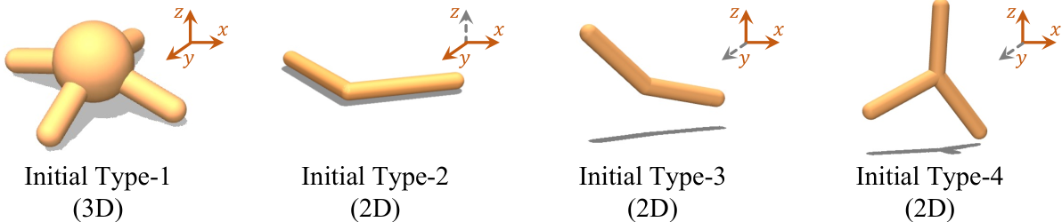
Each episode comprises a morphology-design stage followed by a control stage . Morphology design begins from a task-specific initial morphology , selected from the four structures shown in Figure 8. Over steps, the design policy sequentially updates through morphology-editing actions , first modifying the discrete topology and then updating continuous physical attributes. During topology design, may add or remove a terminal limb or leave the structure unchanged. Each edit must satisfy task-specific upper bounds on tree depth, total limb count, and the number of children per limb, ensuring structurally valid morphologies. The subsequent attribute update specifies limb offsets, capsule radii, attachment positions, and actuator gear ratios. The resulting final morphology remains fixed throughout .
Once the design stage is complete, the simulator instantiates the final morphology as a physical agent and fixes its structural and physical parameters throughout the control stage . At each control step , the policy maps the proprioceptive state , which includes position, linear velocity, and angular velocity, to a continuous motor action . The resulting cumulative task return evaluates the body–brain pair and provides the shared objective for jointly optimizing the design policy and control policy .
B.2 Task-Specific Specifications
We next describe the environment, objective, and design constraints of each task.
Crawler
Crawler evaluates three-dimensional forward locomotion over level terrain. Its initial morphology is the Type 1 initial morphology in Figure 8, comprising a free-floating root body and four primary limbs. The morphology is limited to a tree depth of 4, a total of 29 bodies, and at most two child limbs per body. During attribute design, the root offset remains fixed, while non-root limb offsets are optimized in the – plane within . Capsule radii, attachment positions, and actuator gear ratios are constrained to , , and , respectively.
The reward balances forward velocity and control effort:
| (15) |
where denotes the root position along the forward axis, is the control interval, weights the control penalty, is the number of limbs, and is the continuous motor-action vector. An episode terminates if the root height falls outside or its tilt from the upright orientation exceeds .
Stepper
Stepper evaluates three-dimensional locomotion over a sequence of elevated steps. It uses the Type 1 initial morphology in Figure 8 and shares the topology constraints and continuous attribute ranges of Crawler: a maximum tree depth of 4, at most 29 bodies, and no more than two child limbs per body. The task adopts the forward-velocity and control-effort reward in Eq. (15), with control interval and penalty weight . Because the terrain elevation varies along the course, termination is determined by the root height relative to the local ground surface. An episode terminates if this relative height falls outside or if the root tilt from the upright orientation exceeds . The task therefore favors morphologies with sufficient support, ground clearance, and reach to maintain forward progress across abrupt elevation changes.
Pusher
Pusher evaluates three-dimensional object manipulation using the Type 1 initial morphology shown in Figure 8. The task requires the agent to push a movable cube along the positive -axis while minimizing lateral drift along the -axis. The morphology is constrained to a maximum tree depth of 4, at most 29 bodies, and no more than two child limbs per body. Its continuous attribute ranges are identical to those of Crawler and Stepper.
Let denote the planar coordinates of the cube, and let and denote the three-dimensional positions of the cube and robot root, respectively. The reward is
| (16) |
Here, weights lateral drift, is the control interval, and weights control effort. The four terms reward forward cube motion, penalize lateral drift, encourage robot–cube proximity, and penalize control effort, respectively. An episode terminates if the root height falls outside or its tilt from the upright orientation exceeds .
Cheetah
Cheetah evaluates rapid planar locomotion along the positive -axis. The agent uses the Type 3 initial morphology in Figure 8, comprising a root body and one primary limb arranged in the – plane. The morphology is constrained to a maximum tree depth of 4, at most 14 bodies, and no more than three child limbs per body. Non-root limb offsets are optimized within in the – plane, while capsule radii, attachment positions, and actuator gear ratios are restricted to , , and , respectively.
The reward is defined by the forward velocity of the root:
| (17) |
Here, denotes the root position along the forward axis and is the control interval. An episode terminates if the root height falls outside or if its absolute angular deviation from the upright orientation exceeds .
TerrainCrosser
TerrainCrosser evaluates planar locomotion over discontinuous terrain with repeated gaps. It uses the Type 3 initial morphology in Figure 8 and shares the topology constraints and continuous attribute ranges of Cheetah: a maximum tree depth of 4, at most 14 bodies, and no more than three child limbs per body. The task adopts the forward-velocity reward in Eq. (17), with control interval . Compared with Cheetah, TerrainCrosser imposes a stricter minimum root height. An episode terminates if the root height falls outside or if the absolute root pitch exceeds . The task therefore favors morphologies that combine rapid forward movement with sufficient reach, clearance, and stability to cross gaps.
Swimmer
Swimmer evaluates planar propulsion through a viscous fluid. It uses the Type 2 initial morphology in Figure 8, comprising a root segment connected to one actuated limb in the – plane. The morphology is constrained to a maximum tree depth of 4, at most 14 bodies, and no more than three child limbs per body. Non-root limb offsets are optimized within , while capsule radii, attachment positions, and actuator gear ratios are restricted to , , and , respectively. The task adopts the forward-velocity and control-effort reward in Eq. (15), with control interval and penalty weight . No posture-based early termination is applied; each episode continues until the predefined time horizon.
Glider-Regular
Glider-Regular evaluates planar locomotion within a compact, weakly branching morphology space. It uses the Type 4 initial morphology in Figure 8, comprising a root body and two primary limbs. The morphology is restricted to a maximum tree depth of 3, at most 5 bodies, and no more than one child limb per body, favoring chain-like structures. Limb offsets are optimized within in the task plane, while capsule radii, attachment positions, and actuator gear ratios are constrained to , , and , respectively. The task adopts the forward-velocity reward in Eq. (17), with control interval . An episode terminates if the root height falls outside or if the absolute root pitch exceeds .
Glider-Medium
Glider-Medium uses the same Type 4 initial morphology, environment dynamics, continuous attribute ranges, and termination conditions as Glider-Regular. It also adopts the forward-velocity reward in Eq. (17), with . The maximum tree depth remains 3, while the body limit increases from 5 to 7 and the maximum number of child limbs per body increases from one to two. This larger branching factor introduces a moderately more complex topology space.
Glider-Hard
Glider-Hard further expands the topology space by increasing the body limit from 7 to 9 and allowing up to three child limbs per body, while retaining a maximum tree depth of 3. All other design ranges, environment dynamics, reward, and termination conditions remain unchanged. Together, the three Glider settings provide a controlled evaluation of increasing morphology size and branching complexity under an otherwise identical locomotion objective.
Walker-Regular
Walker-Regular evaluates planar locomotion in a deeper morphology space than the Glider tasks, starting from the Type 4 morphology shown in Figure 8. The design space permits a maximum tree depth of 4, at most 7 bodies, and no more than one child limb per body, thereby favoring deep, chain-like structures. Limb offsets are optimized within in the task plane, while capsule radii, attachment positions, and actuator gear ratios are restricted to , , and , respectively. The task uses the forward-velocity reward defined in Eq. (17), with a control interval of . An episode terminates if the root height falls outside or if the absolute root pitch exceeds .
Walker-Medium
Walker-Medium retains the initial morphology, environment dynamics, continuous attribute ranges, reward, and termination conditions of Walker-Regular. The maximum tree depth remains 4, while the body limit increases from 7 to 15 and the maximum number of child limbs per body increases from one to two. This expanded topology space accommodates both chain-like and moderately branched locomotor structures.
Walker-Hard
Walker-Hard further expands the topology space by increasing the body limit from 15 to 27 and allowing up to three child limbs per body, while retaining a maximum tree depth of 4. The initial morphology, environment dynamics, continuous attribute ranges, reward, and termination conditions remain unchanged. This setting defines the largest planar design space among the Walker tasks and requires coordinated control of a potentially larger and more highly branched articulated body.
Appendix C Method Details
C.1 Algorithm Details
GeCode extends BodyGen (Lu et al., 2025) with a compact Morphogene space for explicit coordination between morphology design and control. The overall procedure comprises two phases. First, a structure-aware RAE is trained offline on randomly generated morphologies to construct the Morphogene space. GeCode then performs Morphogene-driven co-design using a small set of Morphogenes as latent design anchors, which jointly condition the morphology-design and control policies through AdaConcat. During co-design, policy rollouts provide both learning experience and performance statistics for iteratively updating, eliminating, and resampling these anchors. The complete procedure is summarized in Algorithm 1.
C.2 Structural Regularization of the Morphogene Space
As discussed in Sec. 4.1, reconstruction preserves the information required to recover a morphology but does not explicitly organize the latent geometry. We therefore impose two complementary structural regularizers on the morphology codes: a topology-aware contrastive loss for local topology clustering and a tree-structured metric loss for global structural alignment.
For a mini-batch , let denote the morphology code of sample , and let be its -normalized representation. The topology-aware contrastive loss treats morphologies with isomorphic topology graphs as positive pairs:
| (18) |
Here, contains the samples whose topology graphs are isomorphic to that of sample , contains samples with at least one positive pair, and is the temperature parameter. This objective draws morphology codes with the same topology closer while separating those with different topologies.
To preserve finer-grained structural relationships beyond topology classes, we construct a set of index triplets , corresponding to a reference morphology, a structurally similar morphology, and a structurally dissimilar morphology, respectively. The positive index is selected based on a small tree-edit distance from , whereas the negative index is selected based on a large tree-edit distance. The tree-structured metric loss enforces the corresponding reference code to be closer to the positive code than to the negative code by a margin:
| (19) |
Here, denotes the cosine distance between normalized morphology codes, and is the ranking margin.
The complete RAE training objective is
| (20) |
where and control the contributions of the two structural losses.
C.3 Offline and RL-Based Training of the Morphology Decoder
In this work, we learn the morphology latent space using an offline, reconstruction-based RAE decoder, as described in Sec. 4.1. As an alternative, the morphology-design policy can serve as an RL-trained decoder: rather than reconstructing morphology attributes directly, it maps a target morphology code to a morphology through sequential design actions. We describe this alternative below and discuss its trade-offs relative to offline reconstruction.
RL-based Policy Decoding
The morphology-design policy can be trained to decode a target morphology code into a valid design. Starting from an initial morphology , the policy generates topology and attribute design actions conditioned on the current morphology and target code, , yielding the final morphology . We train the policy using the proximity reward in Eq. (10), with the target Morphogene set to . This reward encourages the code of the generated morphology to meet the prescribed similarity threshold with respect to the target code.
RL-based decoding requires simulator rollouts and policy optimization, making pretraining more computationally demanding than direct supervised reconstruction. Moreover, the proximity reward alone does not explicitly impose the pairwise topological and tree-structural relationships encouraged by the regularizers in Eqs. (18) and (19); consequently, it provides less direct control over the organization of the latent space. Its principal advantage is that pretraining also optimizes the morphology-design policy. The pretrained policy can then be carried into co-design, where it continues to generate morphologies while being optimized jointly with the control policy. Accordingly, RL-based decoding incurs higher pretraining cost than offline reconstruction and, without additional structural regularizers, provides less direct control over latent-space organization; in return, it yields a morphology-design policy pretrained for Morphogene-conditioned generation that can be further optimized during co-design.
Appendix D Implementation Details
D.1 Training Details
Following standard reinforcement learning practice, we employ distributed trajectory collection across multiple CPU threads to improve training efficiency. All experiments are conducted with five random seeds on a machine equipped with two NVIDIA GeForce RTX 4090 GPUs. The neural networks are implemented in PyTorch 2.0.1, and the morphology–control environments are simulated using MuJoCo 2.1.0 (Todorov et al., 2012).
D.2 Hyperparameters
GeCode
We implement GeCode in PyTorch on top of BodyGen, retaining its environment, morphology-design space, and policy-optimization settings. To construct the Morphogene space, we train the RAE for 100 epochs on randomly generated valid morphologies using Adam with a learning rate of 5e-4 and a batch size of 2,048. During Morphogene-driven co-design, the morphology encoder remains frozen, while Morphogenes are randomly initialized in the learned latent space and updated after each epoch using existing rollout statistics, without additional environment interactions. Detailed hyperparameters are provided in Table D.2.
| Hyperparameter | Value |
| [2pt][0pt] Morphogene-space Construction | |
| Space construction epochs | 100 |
| RAE batch size | 2,048 |
| RAE Optimizer | Adam |
| RAE learning rate | 5e-4 |
| Limb-token dimension | 128 |
| Morphogene dimension | 32 |
| Attribute reconstruction loss weight | 1.0 |
| Limb-presence mask loss weight | 1.0 |
| Morphology-code regularization weight | 0.01 |
| Topology-aware contrastive loss weight | 8e-3 |
| Contrastive temperature | 0.1 |
| Tree-structured metric loss weight | 0.01 |
| Tree-structured metric margin | 0.2 |
| Maximum tree triplets per batch | 64 |
| [2pt][0pt] Morphogene-Driven Co-design Optimization | |
| Initial Morphogene count | 5 |
| Similarity threshold | 0.4 |
| Proximity reward weight | 1,000 |
| Morphogene update rate | 0.1 |
| Minimum local hits for retention | 5 |
| Top- returns for adaptive sampling () | 5 |
| Policy Transformer depth | 3 |
| Policy Hidden dimension | 64 |
| Value Transformer depth | 3 |
| Value Hidden dimension | 64 |
| Transformer Layer Normalization | Pre-LN |
| Transformer Activation Function | SiLU |
| PPO optimizer | Adam |
| Policy learning rate | 5e-5 |
| Value learning rate | 3e-4 |
| Clip gradient norm | 40.0 |
| PPO clip | 0.2 |
| PPO batch size | 50,000 |
| PPO minibatch size | 2,048 |
| PPO Iterations Per Batch | 10 |
| Training Epochs | 1000 |
| Discount factor | 0.995 |
| GAE parameter | 0.95 |
StackelbergPPO
StackelbergPPO extends BodyGen with a Stackelberg optimization framework (Dai et al., 2026). We follow the official StackelbergPPO implementation: a Fisher regularization coefficient of , up to 20 conjugate-gradient iterations with a relative-error tolerance of , six follower-sampling steps per episode, and a gradient-normalization ratio of .
BodyGen
We follow the official BodyGen implementation (Lu et al., 2025), using Pre-LN MoSAT blocks with SiLU activations, a hidden dimension of 64, and learning rates of 5e-5 and 3e-4 for the policy and value function, respectively. Additional hyperparameters are provided in Table D.2.
Transform2Act
We follow the official Transform2Act implementation (Yuan et al., 2022), using three-layer GraphConv policy and value networks with hidden dimensions (64, 64, 64) and learning rates of 5e-5 and 3e-4, respectively. The policy employs a three-layer, 128-unit JSMLP with Tanh activations, while the value function uses a (512, 256) MLP.
Appendix E Additional Results
E.1 Quantitative Results
Quantitative Performance
Figure 4 presents the learning curves of GeCode and the RL-based baselines, including Transform2Act, BodyGen, and StackelbergPPO, while Table 3 reports the final episode returns as the mean and standard error over five random seeds. GeCode achieves the highest final return in all twelve environments. Relative to the strongest baseline in each task, its improvement ranges from on Swimmer to on Pusher.
The substantial gains on Crawler, Glider-Hard, and Walker-Hard are particularly notable given their large, highly branched morphology spaces. Instead of directly exploring numerous discrete structures, GeCode performs local refinement around individual Morphogene anchors and updates these anchors toward promising regions of the latent space. This local-to-global strategy focuses rollouts on structurally coherent neighborhoods while sharing high-performing design information across anchors, thereby improving exploration efficiency as the morphology space expands.
The gains on Pusher, Stepper, and TerrainCrosser further highlight the importance of explicit body–brain coordination. By conditioning both morphology generation and control on the same Morphogene, GeCode provides the controller with a compact representation of the structural factors underlying the generated body. This shared conditioning enables the controller to adapt its actions to morphology-dependent object contacts, terrain interactions, and stability requirements, while improving credit assignment between body design and control behavior.
In contrast, the smaller gain on Swimmer suggests that explicit body–brain coordination provides a more limited advantage when relatively simple morphologies are already sufficient for effective propulsion. Overall, these results show that GeCode derives its advantage from both structured latent-space exploration and explicit morphology–control coordination, with the benefits becoming more pronounced as structural search and control adaptation grow more tightly coupled.
| Task | NGE | Transform2Act | BodyGen | StackelbergPPO | GeCode |
| (Wang et al., 2019) | (Yuan et al., 2022) | (Lu et al., 2025) | (Dai et al., 2026) | (Ours) | |
| Crawler | 1482.5525.0 | 5396.3177.3 | 8208.6374.3 | 9255.3888.2 | 16143.3583.0 |
| Stepper | 870.6215.5 | 1671.0148.3 | 2087.2243.3 | 2538.9173.6 | 3688.6271.0 |
| Pusher | 551.6120.7 | 571.878.6 | 1809.1162.2 | 3054.4354.9 | 6250.2757.9 |
| Cheetah | 2534.8428.7 | 9542.1635.0 | 11475.1489.5 | 13246.3299.9 | 19888.7944.6 |
| TerrainCrosser | 827.2427.2 | 2426.5654.1 | 4016.4911.6 | 5437.5675.6 | 9670.61176.4 |
| Swimmer | 384.5112.0 | 782.423.6 | 1301.61.3 | 1335.917.2 | 1422.529.5 |
| Glider-Regular | 1567.8756.7 | 6890.4414.8 | 11091.0211.8 | 11429.9261.1 | 23317.5627.9 |
| Glider-Medium | 1649.6763.6 | 8632.01185.1 | 11016.8144.2 | 12652.3222.3 | 22376.4809.9 |
| Glider-Hard | 2081.3348.2 | 6218.5685.9 | 10973.7268.3 | 12110.0330.6 | 19972.8332.1 |
| Walker-Regular | 1402.9595.5 | 7960.6534.2 | 11555.3220.1 | 13216.4536.5 | 24306.11293.0 |
| Walker-Medium | 2600.4481.7 | 7324.4906.8 | 13244.4342.1 | 11764.6418.6 | 21973.3918.9 |
| Walker-Hard | 1504.6553.2 | 4924.0690.3 | 12126.0825.2 | 13643.4597.6 | 21614.6521.8 |
Comparison with Evolutionary Search
Table 3 further compares GeCode with NGE (Wang et al., 2019), an evolutionary method that optimizes populations of embodied designs through selection and variation. GeCode outperforms NGE across all twelve tasks, achieving approximately to the returns of NGE. Evolutionary co-design must distribute a finite interaction budget across numerous morphology candidates and evaluate the controller associated with each design. As the morphology space becomes larger and more highly branched, this population-level evaluation becomes increasingly expensive, while limited knowledge transfer across structurally distinct candidates hinders the joint identification of effective morphologies and compatible controllers.
In contrast, GeCode organizes co-design around a small set of searchable Morphogene anchors in a compact, structurally regularized latent space. Stochastic policy rollouts refine body–brain designs locally around each anchor, while performance-guided updates move the anchors toward promising regions for global exploration. Because all Morphogenes condition the same morphology-design and control policies, knowledge learned from different designs is shared through the policy parameters, while Morphogene updates reuse existing rollout trajectories without additional evaluations. GeCode therefore replaces costly population-level search with structured latent exploration that directly couples morphology refinement and controller adaptation.
E.2 Additional Ablation and Analysis
| Task | ||||||
| Crawler | 0.3384 0.0028 | 0.2928 0.0025 | 0.0010 0.0002 | 0.2558 0.0031 | 5.2215 0.0627 | 0.0267 0.0031 |
| Stepper | 0.3336 0.0058 | 0.2889 0.0060 | 0.0008 0.0001 | 0.2509 0.0085 | 5.1376 0.0280 | 0.0267 0.0048 |
| Pusher | 0.3365 0.0052 | 0.2911 0.0053 | 0.0011 0.0002 | 0.2585 0.0098 | 5.1803 0.0310 | 0.0237 0.0031 |
| Cheetah | 0.0908 0.0025 | 0.0496 0.0024 | 0.0001 0.0000 | 0.2104 0.0030 | 4.7858 0.0152 | 0.0686 0.0017 |
| TerrainCrosser | 0.0919 0.0038 | 0.0496 0.0033 | 0.0002 0.0001 | 0.2410 0.0172 | 4.8627 0.0554 | 0.0720 0.0041 |
| Swimmer | 0.1259 0.0053 | 0.0797 0.0052 | 0.0003 0.0000 | 0.2982 0.0054 | 5.3088 0.0431 | 0.0443 0.0021 |
| Glider-Regular | 0.0736 0.0017 | 0.0189 0.0018 | 0.0000 0.0000 | 0.1544 0.0011 | 6.6390 0.0056 | 0.0000 0.0000 |
| Glider-Medium | 0.0873 0.0138 | 0.0361 0.0128 | 0.0001 0.0000 | 0.2098 0.0174 | 6.1070 0.0800 | 0.0229 0.0139 |
| Glider-Hard | 0.0870 0.0079 | 0.0387 0.0072 | 0.0001 0.0000 | 0.2459 0.0252 | 5.6611 0.0474 | 0.0357 0.0030 |
| Walker-Regular | 0.0783 0.0029 | 0.0285 0.0029 | 0.0001 0.0000 | 0.1782 0.0038 | 5.9831 0.0055 | 0.0087 0.0011 |
| Walker-Medium | 0.1166 0.0030 | 0.0741 0.0026 | 0.0003 0.0000 | 0.2308 0.0111 | 4.8997 0.0504 | 0.0750 0.0041 |
| Walker-Hard | 0.1793 0.0048 | 0.1380 0.0045 | 0.0007 0.0003 | 0.2334 0.0053 | 4.7300 0.0191 | 0.0423 0.0035 |
Analysis of RAE Training
Table 4 reports the task-specific RAE training losses. The consistently small standard errors of the overall objective indicate stable optimization across all twelve environments. The near-zero limb-presence loss shows that the decoder reliably reconstructs variable limb configurations, which is essential for representing morphologies with different topologies. The attribute-reconstruction loss is generally higher for the three-dimensional tasks, including Crawler, Stepper, and Pusher, reflecting the greater complexity of their geometric representations. Across the Glider and Walker task groups, generally increases as the branching constraints are relaxed, consistent with the greater morphological diversity admitted by the more challenging variants.
The topology-aware contrastive loss and tree-metric loss impose complementary structure on the latent space. Specifically, organizes morphology codes into coherent local neighborhoods according to topology, preventing structurally distinct morphologies from becoming arbitrarily entangled. In contrast, preserves graded structural relationships by ordering latent distances according to tree-edit similarity, such that nearby codes correspond to progressively related morphology structures. The consistently small standard errors indicate stable optimization of both objectives across environments. Moreover, the near-zero on weakly branching tasks such as Glider-Regular and its larger values in more structurally diverse tasks reflect the increasing difficulty of preserving global structural order as branching complexity grows. Together, these losses balance topology-aware local clustering with globally meaningful distance organization, enabling Morphogene updates to traverse the latent space through coherent structural variations.
| Limb Diversity | Relative Modulation | Between-Limb Energy Ratio | ||||
| Task | AdaConcat | Direct Concat | AdaConcat | Direct Concat | AdaConcat | Direct Concat |
| Crawler | 0.658 0.053 | 0.000 | 0.482 0.041 | 0.000 | 0.181 0.020 | 0.000 |
| Stepper | 0.746 0.126 | 0.000 | 0.542 0.096 | 0.000 | 0.203 0.049 | 0.000 |
| Pusher | 0.643 0.047 | 0.000 | 0.480 0.036 | 0.000 | 0.165 0.017 | 0.000 |
| Cheetah | 1.257 0.081 | 0.000 | 0.841 0.050 | 0.000 | 0.346 0.034 | 0.000 |
| Terraincrosser | 1.328 0.119 | 0.000 | 0.894 0.076 | 0.000 | 0.365 0.025 | 0.000 |
| Swimmer | 1.169 0.165 | 0.000 | 0.772 0.110 | 0.000 | 0.334 0.035 | 0.000 |
| Glider-Regular | 2.288 0.537 | 0.000 | 1.522 0.309 | 0.000 | 0.410 0.068 | 0.000 |
| Glider-Medium | 1.328 0.191 | 0.000 | 0.876 0.106 | 0.000 | 0.350 0.061 | 0.000 |
| Glider-Hard | 1.319 0.362 | 0.000 | 0.862 0.229 | 0.000 | 0.336 0.071 | 0.000 |
| Walker-Regular | 1.453 0.140 | 0.000 | 0.968 0.070 | 0.000 | 0.384 0.037 | 0.000 |
| Walker-Medium | 1.031 0.136 | 0.000 | 0.714 0.112 | 0.000 | 0.290 0.039 | 0.000 |
| Walker-Hard | 1.275 0.090 | 0.000 | 0.865 0.076 | 0.000 | 0.369 0.016 | 0.000 |
Analysis of Limb-Specific Conditioning in AdaConcat
Figure 10 shows that AdaConcat produces distinct limb-level conditions from the same Morphogene while preserving feature patterns shared across the body. By contrast, direct concatenation provides every limb with an identical Morphogene, requiring the policies to infer limb-specific distinctions from other inputs. Complementing the performance comparison in Table 1, the learning curves in Figure 11 show that GeCode generally outperforms this direct-concatenation variant, with pronounced gains on Pusher and Walker-Regular. These results suggest that adapting the shared Morphogene to each limb helps the policies account for differing roles, such as object contact and locomotor support, during morphology design and control.
To quantify the limb specificity of AdaConcat, we use three complementary measures. Let denote the limb-specific condition produced by AdaConcat from for limb . Limb Diversity is the mean pairwise distance between limb conditions, normalized by the magnitude of :
Relative Modulation measures the average deviation of the limb-specific conditions from the shared Morphogene, normalized by its magnitude:
Between-Limb Energy Ratio measures the proportion of total condition energy associated with variation across limbs:
Table 5 shows that AdaConcat consistently produces distinct limb-specific conditions from a shared Morphogene. Nonzero Relative Modulation indicates that these conditions differ from the shared Morphogene, while nonzero Limb Diversity and Between-Limb Energy Ratio show that the transformation varies across limbs. Between-limb variation accounts for – of total condition energy, indicating substantial limb specificity while retaining a shared component. In contrast, all three measures are zero under direct concatenation, which provides every limb with the same unmodified Morphogene.
| Task | Threshold (BodyGen) | GeCode | StackelbergPPO | BodyGen | Transform2Act | NGE | ESS |
| Crawler | 8208.57 | 14.35 M | 31.10 M | 49.45 M | |||
| Stepper | 2087.16 | 20.90 M | 31.20 M | 45.80 M | |||
| Pusher | 1809.06 | 14.20 M | 24.20 M | 48.20 M | |||
| Cheetah | 11475.06 | 15.05 M | 25.15 M | 45.40 M | |||
| TerrainCrosser | 4016.37 | 14.05 M | 24.75 M | 50.00 M | |||
| Swimmer | 1301.57 | 8.05 M | 14.70 M | 36.75 M | |||
| Glider-Regular | 11091.03 | 8.65 M | 28.00 M | 49.85 M | |||
| Glider-Medium | 11016.82 | 10.55 M | 26.10 M | 44.75 M | |||
| Glider-Hard | 10973.74 | 12.65 M | 19.70 M | 40.30 M | |||
| Walker-Regular | 11555.34 | 12.90 M | 18.80 M | 50.00 M | |||
| Walker-Medium | 13244.43 | 15.35 M | 46.25 M | ||||
| Walker-Hard | 12125.98 | 15.45 M | 22.25 M | 46.55 M | |||
| Task | Threshold (StackelbergPPO) | GeCode | StackelbergPPO | BodyGen | Transform2Act | NGE | ESS |
| Crawler | 9255.29 | 16.30 M | 46.30 M | ||||
| Stepper | 2538.91 | 26.65 M | 42.75 M | ||||
| Pusher | 3054.39 | 21.40 M | 48.85 M | ||||
| Cheetah | 13246.30 | 17.55 M | 37.25 M | ||||
| TerrainCrosser | 5437.52 | 18.35 M | 50.00 M | ||||
| Swimmer | 1335.90 | 11.20 M | 37.05 M | ||||
| Glider-Regular | 11429.94 | 9.20 M | 30.35 M | ||||
| Glider-Medium | 12652.30 | 12.80 M | 44.35 M | ||||
| Glider-Hard | 12110.01 | 14.75 M | 29.60 M | ||||
| Walker-Regular | 13216.44 | 14.70 M | 27.85 M | ||||
| Walker-Medium | 11764.57 | 13.65 M | 43.05 M | 24.05 M | |||
| Walker-Hard | 13643.36 | 17.10 M | 39.30 M |
E.3 Sample and Training Efficiency
Sample Efficiency
We measure sample efficiency by the number of environment interactions required to reach task-specific thresholds, defined by the highest returns attained during training by BodyGen and StackelbergPPO. As shown in Table 6, GeCode reaches both thresholds with the fewest interactions in all twelve tasks. Summed across tasks, GeCode requires 48.06% and 57.69% fewer interactions than the fastest task-specific baseline to reach the BodyGen and StackelbergPPO thresholds, respectively. For example, it reaches the BodyGen threshold on Glider-Regular in 8.65M interactions, compared with 28.00M for the fastest baseline. GeCode also reaches every StackelbergPPO threshold within the 50M-interaction budget, whereas BodyGen reaches only one.
This efficiency arises from the complementary roles of local rollouts and global Morphogene updates. Rollouts explore related body designs around each Morphogene, providing more consistent experience for the conditioned controller. Performance-guided updates and adaptive sampling subsequently direct interactions toward promising regions of the Morphogene space. Because these operations reuse policy-training trajectories, they improve the focus of exploration without additional environment interactions.
| Task | Space Size (max) | GeCode | StackelbergPPO | ||
| Offline RAE Training | Co-design Optimization | Total Time | |||
| Crawler | 29 | 0.997 0.017 | 30.755 3.390 | 31.752 3.389 | 27.924 1.617 |
| Stepper | 29 | 1.027 0.020 | 29.560 3.583 | 30.587 3.566 | 30.969 1.346 |
| Pusher | 29 | 1.028 0.022 | 22.754 4.045 | 23.782 4.031 | 25.447 1.811 |
| Cheetah | 14 | 0.767 0.003 | 21.384 0.676 | 22.151 0.679 | 19.959 0.205 |
| TerrainCrosser | 14 | 0.883 0.023 | 24.279 1.040 | 25.161 1.033 | 24.020 1.441 |
| Swimmer | 14 | 0.839 0.017 | 17.948 1.214 | 18.787 1.220 | 20.913 0.748 |
| Glider-Regular | 5 | 0.877 0.024 | 19.320 0.809 | 20.197 0.789 | 19.319 0.379 |
| Glider-Medium | 7 | 0.861 0.025 | 19.316 0.212 | 20.178 0.211 | 20.494 0.951 |
| Glider-Hard | 9 | 0.839 0.023 | 19.728 0.805 | 20.567 0.787 | 21.072 0.939 |
| Walker-Regular | 7 | 0.878 0.020 | 18.338 0.692 | 19.216 0.685 | 22.691 0.417 |
| Walker-Medium | 15 | 0.823 0.023 | 18.960 0.424 | 19.783 0.405 | 24.666 0.899 |
| Walker-Hard | 27 | 1.014 0.016 | 22.248 2.395 | 23.263 2.388 | 23.574 0.476 |
| Average | 22.952 0.760 | 23.421 0.514 | |||
| Task | Eval. Return | Params. (M) | Latency (ms) | FLOPs (M) | FLOPs (Per Limb) (M) |
| Crawler | 15899.313 619.609 | 0.5522 | 16.734 0.759 | 9.354 | 0.323 |
| Stepper | 3336.782 335.130 | 0.5522 | 31.431 8.901 | 7.617 | 0.319 |
| Pusher | 6019.497 688.621 | 0.5524 | 13.951 0.970 | 8.682 | 0.321 |
| Cheetah | 20130.416 1012.861 | 0.5517 | 1.511 0.766 | 2.195 | 0.305 |
| TerrainCrosser | 9760.178 1195.632 | 0.5518 | 12.976 11.144 | 2.385 | 0.305 |
| Swimmer | 1438.432 25.512 | 0.5517 | 1.743 1.113 | 2.319 | 0.305 |
| Glider-Regular | 23770.548 668.018 | 0.5515 | 0.635 0.049 | 1.514 | 0.303 |
| Glider-Medium | 22664.985 821.074 | 0.5515 | 0.607 0.032 | 1.945 | 0.304 |
| Glider-Hard | 20096.701 302.635 | 0.5515 | 0.616 0.002 | 2.441 | 0.305 |
| Walker-Regular | 24500.695 1315.028 | 0.5517 | 0.614 0.039 | 2.070 | 0.304 |
| Walker-Medium | 22144.726 950.681 | 0.5517 | 14.692 12.166 | 2.824 | 0.306 |
| Walker-Hard | 21732.894 543.298 | 0.5517 | 45.465 12.229 | 3.072 | 0.307 |
Training Efficiency
GeCode maintains competitive training efficiency, with wall-clock costs comparable to—and often lower than—those of StackelbergPPO across the evaluated tasks. As shown in Table 7, offline RAE training requires only between and hours of wall-clock time, accounting for less than of GeCode’s overall training time and thus introducing minimal computational overhead. During co-design, Morphogene updates reuse trajectories collected for policy optimization and involve only morphology encoding and lightweight latent-space operations, requiring neither additional environment interactions nor nested policy-optimization procedures.
Table 7 shows that GeCode incurs moderately higher wall-clock costs on three-dimensional tasks such as Crawler, while demonstrating a clear efficiency advantage on two-dimensional planar tasks, particularly Glider and Walker. The additional cost on three-dimensional tasks arises primarily from the greater complexity of the morphologies discovered by GeCode, rather than from the Morphogene update procedure itself. By exploring broader regions of the design space, GeCode identifies higher-performing and structurally richer agents with more limbs than StackelbergPPO. These larger morphologies increase simulation cost and produce longer limb-token sequences for Transformer processing, thereby extending policy-optimization time. The increased wall-clock cost therefore reflects GeCode’s ability to explore more complex morphology regions, rather than substantial overhead from its latent-space search mechanism.
On two-dimensional planar tasks such as Walker, where the generated morphologies are comparable in scale to those of StackelbergPPO, GeCode incurs lower computational cost. This advantage reflects the computational efficiency of Morphogene-space optimization. Unlike StackelbergPPO, which incorporates follower updates and second-order optimization, GeCode performs lightweight, performance-guided latent updates using existing rollout statistics. Its optimization overhead therefore remains small, with the overall computational cost determined primarily by morphology complexity rather than the Morphogene update procedure.
Inference Efficiency
Table 8 demonstrates that GeCode remains computationally lightweight during evaluation. Its parameter count is nearly constant across tasks at approximately M, reflecting the use of shared morphology-design and control networks rather than morphology-specific models. Total computation ranges from M to M FLOPs per control decision, primarily reflecting differences in the number of limbs processed. Notably, the per-limb cost remains within a narrow range of M–M FLOPs, indicating that inference scales predictably with morphology size. GeCode therefore supports structurally diverse agents without introducing design-specific networks or substantial inference overhead.
E.4 Visualization
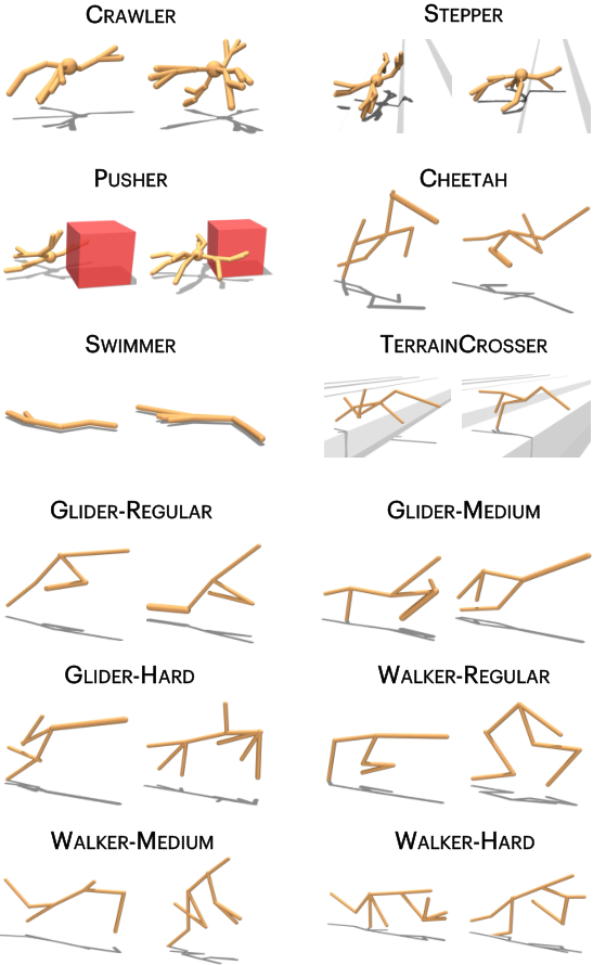
Morphologies Discovered by GeCode
Figure 12 presents representative morphologies discovered by GeCode across the evaluated environments. The generated agents exhibit substantial diversity in topology, limb arrangement, and body proportions, ranging from compact locomotor structures to highly branched designs for complex-terrain traversal and object manipulation. Rather than remaining confined to minor variations of the initial morphology, Morphogene-driven exploration enables GeCode to reach structurally distinct yet task-appropriate regions of the design space. The diversity and validity of these agents demonstrate that GeCode provides broad morphology-space coverage while preserving the realizability and functional relevance of the discovered designs.

Visualization of Structural Organization in the Morphogene Space
Figure 13 examines whether distances between morphology codes reflect meaningful structural relationships. The pairwise distance matrices exhibit clear block and graded patterns aligned with morphology complexity, topology, and limb configuration. Morphologies with similar limb counts and branching structures form compact latent neighborhoods, whereas structurally distinct designs are separated by larger distances. This organization is particularly evident in the Glider variants, where morphologies with the same limb count form low-distance blocks. In broader design spaces, such as Crawler, Stepper, and Walker-Hard, latent distances generally increase as structural complexity and branching patterns diverge. Variations within the same limb-count group further show that the representation captures finer geometric and connectivity differences beyond body count. These results demonstrate that the learned latent space places structurally similar morphologies close together while separating increasingly different designs. This organization supports Morphogene-driven co-design by enabling coherent local exploration around each Morphogene and structured global exploration through performance-guided updates.

Visualization of Morphogene Update Trajectories
Figure 14 shows that valid morphology codes form distinct clusters associated with structural complexity, indicating that the learned latent spaces preserve meaningful morphological relationships. During co-design, Morphogenes follow task-dependent trajectories through this structured support rather than moving as unconstrained latent perturbations. In broad design spaces, such as Crawler, Cheetah, and Walker-Hard, different Morphogenes traverse complementary regions and reach morphology families with varying structural complexity. Progressive elimination of underperforming Morphogenes then concentrates the rollout budget on promising regions while retaining diversity among the surviving trajectories.
These trajectories reveal how GeCode integrates local and global exploration. Stochastic rollouts refine morphology variations around each Morphogene, whereas performance-guided updates move the Morphogenes across broader regions of the latent space. Consequently, a small Morphogene set can efficiently cover diverse yet structurally coherent morphology families without exhaustively evaluating independent designs.
Appendix F Discussion
F.1 Comparison with UNIMAL
Morphology Design Spaces
UNIMAL (Gupta et al., 2021) provides a well-structured design space for articulated agents, with constrained limb addition, deletion, and continuous attribute mutations that support diverse yet physically valid morphologies. Its explicit mutation operators offer a systematic basis for studying how body structure affects locomotion performance. The BodyGen-based benchmark adopted in this work supports comparable design operations but evaluates co-design across twelve task-specific environments spanning 2D and 3D locomotion, uneven-terrain traversal, and object manipulation. Each environment specifies its own initial morphology, task objective, and structural constraints. Together, these settings admit a wider variety of viable designs—from compact planar agents to larger, highly branched bodies—and impose different demands on the controllers that operate them.
The BodyGen-based benchmark permits larger and more diverse morphologies than UNIMAL. Although both benchmarks initialize Crawler with an ant-like structure, the design space used here allows up to 29 limbs, compared with UNIMAL’s limit of 10. Within the Glider and Walker families, progressively relaxed branching limits further expand the range of possible topologies while preserving each task objective. Together, the BodyGen-based environments test whether a co-design method can explore structurally diverse morphologies and learn compatible controllers under distinct task demands. By expressing topology edits and attribute updates as sequential actions evaluated through policy rollouts, the benchmark also provides a natural setting for RL-based morphology design and for assessing how effectively task feedback guides body–brain co-adaptation.
Search Methods and Computational Cost
Methods using the UNIMAL design space address morphology-evaluation costs differently. DERL (Gupta et al., 2021) evolves individual morphologies and trains a controller for each candidate, making fitness evaluation expensive. LOKI (Jeon et al., 2025) reduces this burden by sharing controllers among clusters of similar morphologies and exploring new designs through dynamic local search. Both approaches nevertheless search over explicit morphology candidates, whose performance must be evaluated as exploration proceeds.
GeCode instead organizes exploration around a small set of anchors in the compact Morphogene space. Conditioned rollouts explore body–controller designs locally around each anchor, while performance-guided updates move the anchors toward promising latent regions. Because these rollouts also train the shared design and control policies and provide the returns used for anchor updates, GeCode requires neither candidate-specific controller training nor a separate evaluation loop for global latent-space exploration, thereby balancing effective co-design with negligible additional computational cost (see App. E.3 for a detailed efficiency analysis).
F.2 Limitations and Future Work
In this section, we discuss the limitations of the current framework and outline directions for extending Morphogene-driven co-design.
(1) Scaling to highly diverse morphologies.
GeCode shares a control policy across Morphogenes, allowing experience to transfer between related designs. Early in training, however, the explored morphologies may differ substantially in topology and dynamics. A shared controller with limited capacity may learn some bodies more readily than others, biasing their observed returns and, in turn, the performance-guided Morphogene updates. GeCode partly mitigates premature concentration by incorporating the best locally generated morphology code into each anchor update, thereby preserving anchor-specific exploration. This does not fully remove biases arising from unequal controller adaptation. Future work could use Morphogenes to guide knowledge routing or modular policy selection (Feng et al., 2026; Xie et al., 2026; Xie et al., 2025), enabling specialization across body structures while retaining the benefits of shared learning.
(2) Shared Morphogene Spaces Across Tasks. The Morphogene space is constructed from morphological structure and geometry rather than task rewards, suggesting that it may capture body-level factors shared across tasks. In this study, we construct the space and train the policies separately for each environment. Although offline Morphogene-space construction requires no environment interaction and incurs modest computational cost, whether Morphogenes can transfer to new objectives or terrains remains an open question. Future work could investigate a shared Morphogene space across compatible design domains, together with task-adaptive conditioning that reuses body-level knowledge while adapting morphology generation and control.
(3) Physical deployment. Like much of morphology–control co-design research, GeCode is evaluated in simulation using MuJoCo (Todorov et al., 2012). Extending such methods to physical robots remains challenging: exploring diverse body structures requires fabrication or reconfigurable hardware, while most available robot platforms have fixed morphologies, such as humanoid (Cao, 2025; Liu et al., 2026) and quadruped designs (Han et al., 2024; Long et al., 2024). Fabrication constraints, actuator limits, and differences between simulated and real contact dynamics further complicate deployment. Our results demonstrate Morphogene-driven co-design in simulation rather than on hardware. Nevertheless, Morphogene’s compact representation of coordinated body–brain designs could help identify promising structural features and control requirements, providing guidance for the design and fabrication of physical robots.