Observing Phase Space Evolution During Unimolecular Decay
Abstract
Direct time-resolved observation of large amplitude dynamics during ground state statistical unimolecular decay remains an experimental challenge. Here, an experimental Time-Resolved Coulomb Explosion Imaging (TR-CEI) study (J. Chem. Phys. 151, 174301, 2019) of the canonical unimolecular reaction NO2 NO( + O() at threshold dissociation energies is modeled and analyzed. Quasi-classical trajectory (QCT) simulations on an accurate and validated ground state potential energy surface (PES), with energy and angular momentum constraints from known product state distributions, are used to characterize the dissociation dynamics. TR-CEI projects suddenly, via ultrafast Strong Field Ionization (SFI), the evolving neutral ground state wavepacket onto the repulsive doubly charged cationic state which then impulsively fragments into the NO+ + O+ ion pair. Within the Coulomb recoil approximation, which applies at longer NO–O (Jacobi) separations, the ion pair CEI-energy is inversely proportional to the scalar distance between the neutral ground state NO and O moieties at the moment of SFI, thus providing a direct measure of the evolving average NO–O distance during unimolecular decay. Results from QCT simulations agree favourably with the TR-CEI measurements. Phase space evolution, recurrence time distributions and Lyapunov exponent analysis are presented which support the conclusion that TR-CEI directly observes phase space evolution during unimolecular decay. For the present system, the time scale for the phase space distribution to achieve statisticality is estimated to be 2 to 3 ps.
1 Introduction
The characterization of ground state unimolecular photodissociation
dynamics near dissociation thresholds remains a challenging problem
due to the extreme density of states, large amplitude motion,
overlapping resonances and long decay times. A commonly accepted
treatment is that of statistical unimolecular decay: the available
microcanonical phase space is rapidly filled on a time scale short
compared to that of the reaction, requiring that intramolecular
vibrational energy redistribution (IVR) be both fast and complete on
the reaction time scale.Baer and Hase (1996) This ”ergodicity”
assumption greatly simplifies the calculation of reaction rates, but
it remains a fundamental question, whether the dynamics are truly or
only apparently statistical.Remacle and Levine (1991); Remacle and Levine (1998) Apparent
agreement with statistical theories may depend on the chosen
observable, such as a state-resolved rate or product state
distributions. Since the filling of phase space takes time, the
dynamics cannot be ”instantaneously” statistical. Different
observables may exhibit different timescales for the onset of
statisticality. It is therefore desirable to develop experimentally
accessible observables which are not only sensitive to the final
products, but directly probe their phase space evolution during
unimolecular decay.
A standard approach to preparing a microcanonical ground state
distribution is via photoabsorption to an electronically excited state
which undergoes extremely rapid (i.e., fs) internal conversion
to the ground electronic state, thus converting photon energy into
ground state vibrational energy - a so-called “hot” molecule which
then proceeds to dissociate on the ground state potential surface
(PES). In a time-resolved experiment, an ultrashort pump pulse is used
and a delayed ultrashort probe pulse generates an observable (e.g.,
photofragment yield). Here, the temporal region between initial
photoinduced “hot” ground state formation and the final appearance
of free products is considered. Can an observable be constructed which
probes this highly complex large amplitude motion region as the system
evolves towards a loose transition state and the subsequent emission
of free products?
Time-Resolved Coulomb Explosion Imaging (TR-CEI) has emerged as a
novel probe of unimolecular decay
dynamicsEndo et al. (2020); Ding et al. (2019b) and was recently applied
to the threshold photodissociation dynamics of
NO2.Ding et al. (2019b) In that experiment, an ultrashort pump pulse
at 400 nm excited NO2 to its optically bright state, an
internal energy corresponding to the NO2 NO( + O() dissociation threshold of
cm-1 (397.954 nm). Jost et al. (1996) Ultrafast
internal conversion subsequently leads to formation of the “hot”
electronic ground
state.Arasaki and Takatsuka (2007); Arasaki et al. (2010); Forbes et al. (2017); von Conta et al. (2018) By
50-60 fs, a complex ground state wavepacket has formed, with
population transfer to the ground state largely complete by 250
fs. These non-adiabatic processes are the initial dynamics in the
formation of the “hot” ground state NO2 molecule, designated here
as [NO2]∤, which is understood to subsequently undergo
strong IVR and very large amplitude motions. In the following, only
slightly longer time scales wherein NO2 can be treated as a “hot”
ground state molecule are considered.
In TR-CEI, the SFI probe pulse projects the evolving neutral ground
state wavepacket onto the repulsive doubly charged cationic state
which then fragments into NO+ + O+ ion pairs. Within the
Coulomb recoil approximation, which becomes accurate at longer NO–O
distances, the ion pair recoil energy is inversely proportional to the
scalar distance (Jacobi coordinates) between the neutral ground state
NO and O moieties at the moment of SFI, thus providing a measure of
the evolving average NO–O distance during unimolecular decay. TR-CEI
is a potentially unique measure of large amplitude ground state phase
space evolution during statistical unimolecular decay. In the
following, the TR-CEI experiment is analyzed through a combination of
quasi-classical trajectory (QCT) simulations and detailed phase space
analysis.
NO2 is a well-suited system to the study of statistical
vs. non-statistical photodissociation dynamics because the NO2
NO+O channel is accessible near threshold, where small
changes in excess energy strongly affect fragmentation. State-specific
near-threshold experiments showed that individually prepared states
can exhibit distinct unimolecular decay behavior rather than perfectly
averaged statistical fragmentation.Miyawaki et al. (1993)
Product-state-resolved measurements of NO fragments provide
rotational, vibrational, and translational distributions which
directly test statistical phase-space
predictions.Hunter et al. (1993) Time-resolved
unimolecular-decomposition experiments further connected fragment
observables to the evolving dissociation dynamics near the NO2
NO+O transition
region.Ionov et al. (1993) Since NO2 is triatomic,
full-dimensional potential-energy surfaces and detailed dynamics
studies are feasible, while the dynamics remain nontrivial. Schinke
and co-workers established NO2 as a paradigm for comparing
classical trajectory calculations with RRKM and statistical adiabatic
channel models on a global ground-state PES
Grebenshchikov et al. (1999). This renders NO2
especially useful for testing the statistical assumption that
intramolecular vibrational redistribution is indeed fast compared with
bond fission. NO2 is an ideal case because the decades of
dedicated, ongoing experimental and theoretical work provide
information about state-resolved photofragmentation and time-resolved
imaging. This makes NO2 microcanonical dynamics a stringent test of
whether the photofragmentation is statistical or if it retains mode-
or state-specific dynamical
memory.Grebenshchikov et al. (1999); Hunter et al. (1993); Ding et al. (2019a)
A wide range of potential energy surfaces (PESs) for the reactive O+NO
system has been developed each tailored for different
applications. For example, the vibrational state-dependent cross
sections were calculated from dynamics
studies.Caridade and Varandas (2004); Duff et al. (1994); Ramachandran et al. (2000) One
PESDuff et al. (1994) for the 2A′ state was used a fit to electronic
structure calculations at the complete active space SCF (CASSCF)
level, followed by multireference contracted configuration interaction
and a modified Duijneveldt (11s6p) basis set.Walch and Jaffe (1987) Another
PES was based on 1250 (for the 2A′) and 910 (4A′) CASPT2
point calculations, with fitting to an analytical
function.Sayós et al. (2002) Such an approach was also used for the
2A′′ state.González et al. (2001) Complementarily, a PES for the
2A′ state using a diatomics in molecules (DIM) expansion with the
two-body terms was based on extended Hartree-Fock
calculations.Varandas (2003) A 2-dimensional PES with the NO bond
length fixed at its equilibrium value of 2.176 a0 was determined at
the icMRCI+Q and cc-pVQZ level of theory and represented as a cubic
spline.Ivanov et al. (2007) This work also presented a PES for the
2A′′ state. More recently, a double many body expansion fit to
1700 points at the MRCI/aug-cc-VQZ level of theory for the 2A′′
state was carried out.Mota et al. (2012) In addition, QCT
simulationsCaridade and Varandas (2004); Castro-Palacio et al. (2014); Bose and Candler (1997); Sayós et al. (2002)
were reported for the temperature dependent rate for the
N(4S)+O2 NO+O and its reverse reaction using
different PESs. Most recently, two machine learning-based PESs were
reported. One of them used CASPT2 reference data and was represented
as a many body permutation invariant polynomialVarga and Truhlar (2021)
whereas the other used MRCI+Q calculations as the reference method,
together with a reproducing kernel Hilbert space (RKHS)
representation.San Vicente Veliz et al. (2020); Unke and Meuwly (2017)
The present study differs in emphasis from previous work which studied
the non-adiabatic dynamics on somewhat lower-level
CASSCF/cc-pVTZ-quality PESs between the X2A1/A2B2
states.Arasaki and Takatsuka (2007) There, an initial wavepacket on the ground
state was projected onto the electronically excited state and
propagated through the conical intersection (CI). After reaching this
crossing, one part of the wavepacket switched to the ground electronic
state whereas the remainder continues on the excited state PES. Upon
reaching the CI for a second time, again a fraction switches to the
ground state. It was reported that after fs most of the
excited state population transferred to the ground state, forming
[NO2]∤, from where dissociation into NO+O was followed in a
fashion comparable to the present work but no specific observable was
constructed which permits following the dynamics to long range. Hence,
differences between the present work and earlier simulations concern
(i) non-adiabatic effects, which were not included here since the
focus is on the hot ground state [NO2]∤ after all
non-adiabatic dynamics are complete, and (ii) the accuracy of the
underlying PES(s) which is higher in the present work.
This manuscript is structured as follows. First, the theory and
simulation methods are presented, followed by characterization of the
low-energy collision process, final product rotational distributions
and the details of ensemble of reactive trajectories. The trajectory
data were used to model the TR-CEI experiments, permitting a direct
comparison of experiment with theory. A phase space analysis is
presented, including the sampling of individual trajectories,
recursion time distributions and Lyapunov exponents. Finally,
conclusions are drawn supporting the case that TR-CEI probes the
progressive loss of dynamical memory and the emergence of statistical
behavior in unimolecular dissociation of NO2.
2 Methods
2.1 The Potential Energy Surface
Reference calculations for the 2A′ state of NO2 connecting the
N(4S) + O2(X O(3P) +
NO(X states were carried out at the MRCI+Q/aug-cc-pVTZ level
of theory, based on CASSCF calculations including all valence orbitals
in the active space. For the O+NO and N+O2 channels, the grid
contained 7280 and 3920 geometries, respectively. The individual
channels (OA + NOB, OB + NOA, and
N + OAOB) were mixed using a distance-dependent
exponential switchingKoner et al. (2020) for which a separate mixing
data set was constructed. For on- and off-grid points the
with corresponding RMSE-values of 0.02 eV (0.5 kcal/mol) and 0.03 eV
(0.7 kcal/mol), respectively.San Vicente Veliz et al. (2020) Details about other
PESs for the N+O2 system are provided in the supporting
information.
2.2 Quasi-Classical Trajectory Simulations
The QCT method used in this work has been thoroughly described in the
literature.Karplus et al. (1965); Truhlar and Muckerman (1979); San Vicente Veliz et al. (2020); Veliz et al. (2021) In
this approach, Hamilton’s coupled differential equations of motion are
integrated using the fourth-order Runge–Kutta method in reactant
Jacobi coordinates with a time step of fs, ensuring
conservation of total energy to within per
trajectory. After adequate time propagation by monitoring the
internuclear distances, the momenta and positions are transformed to
the appropriate coordinate system (i.e., product Jacobi coordinates if
a product is formed). In order to simulate the TR-CEI pump-probe
experiment, a procedure was developed for generating the initial
() energized NO2 ground state configuration with internal
energy and angular momenta constraints. This required a
“synchronization” of the trajectories, as described below.
A total of 500 000 quasi-classical trajectories were computed on the
NO2 PESSan Vicente Veliz et al. (2020) for the initial rovibrational state
. The initial reactant separation for the O + NO
collision was set to 22 . The translational energy was equivalent
to a temperature of 50 K to generate the “hot” parent species
[NO2]∤. For this, the impact parameter was selected
using stratified samplingTruhlar and Muckerman (1979); Bender et al. (2015); Koner et al. (2018) in
the range . To determine , the
opacity function for the exchange reaction was
determined, see Figure S1. Possible elementary
processes used for classification included elastic, inelastic and atom
exchange trajectories. In addition to atom exchange (see above), a
collision was classified as elastic/inelastic if the final NO-state
was , and , respectively.
The final angular momentum of the product diatomic species was obtained from the final position and momentum . To determine the rotational quantum number as a real value, the following quadratic expression was solvedTruhlar and Muckerman (1979); Karplus et al. (1965):
| (1) |
The vibrational quantum number () of the final diatomic species was subsequently determined as a non-integer value according toTruhlar and Muckerman (1979); Karplus et al. (1965):
| (2) |
where denotes the diatomic bond length, and
represent the turning points of the diatomic species on the effective
potential corresponding to rotational state for internal energy
, is the reduced mass, and is the
diatomic potential energy curve.
Simulations using measured : In addition to standard
Boltzmann-type initial conditions for the NO-angular momentum ,
simulations were also performed by using experimentally measured
from photofragment yield spectroscopy.Reid et al. (1994) The
impact parameter for each trajectory was computed according to where is the rotational
quantum number sampled from the probability distribution reported in
Reisler’s work, is the reduced mass defined as the mass of the
oxygen atom divided by the total mass of the nitrogen and oxygen
atoms, and is the translational energy. The translational energy
was sampled from a Gaussian distribution centered at eV with a width of eV, representing
the energy spread. The number of initial conditions assigned to each
value was proportional to the experimentally measured probability
in the distribution.
2.3 Analysis
In order to simulate the TR-CEI pump-probe experiments, a “start
time” was required for the creation of the energized ground state
[NO2]∤ molecule. Thus, for subsequent analyses, all
trajectories were first synchronized to have a common ”time zero”
(), which was defined as the instance at which for
the first time. Here, is the distance (Jacobi coordinates) between
the incoming oxygen atom OB and the center of mass of the
diatomic NOA, and a0. The ”lifetime”
of metastable [NO2]∤ was then determined
according to Figure 1.
3 Results
In the following, first the final state distribution after preparation
of the near-dissociative initial conditions and the dynamics in the
hot [NO2]∤ complex are analyzed. This is followed by the
calculation of the time- and energy-resolved NO+ + O+ Coulombic
recoil energy maps which correspond to the TR-CEI
experiments. Finally, the phase space trajectories are analyzed.
3.1 Breakup and Final State Analysis
The initial collision system was prepared in a metastable-dissociative
state which emulates the preparation of the “hot” ground state
molecule in the TR-CEI experiments. The opacity function shown in
Figure S1 shows that the initial conditions chosen
cover the relevant collision parameters. In other words, the reaction
probability decays to zero for a0.

The first property considered was the lifetime distribution
of the [NO2]∤ collision complex, shown in Figure
2. As the final state is the O+NO channel, two
possibilities exist: elastic/inelastic scattering for which OA + NOB OA + NOB or atom
exchange, characterized by OA + NOB
OB + NOA. Analysis of the 500 000 trajectories
showed that 216 249 trajectories formed the hot [NO2]∤
complex after synchronization. Amongst these, 44% resulted in
exchange, 55% in inelastic scattering, and 1% in elastic
scattering.

Next, the product rotational state distributions were
analyzed. Because the collision energy is low (50 K) and the initial
NOB is in , vibrational excitation of the product
cannot occur: the vibrational quantum number is conserved by the
collision. Hence, the product state is fully characterized by the
relative kinetic energy of the O and NO fragments and . Figure
3 presents the dependence of on the
[NO2]∤ lifetimes, ranging from ps
(blue) to ps (indigo). Typically, with
increasing lifetime, the maximum of shifts to higher
values. This is most clearly seen when comparing for
ps (blue) with ps (red) for
which and ,
respectively. For the longest lifetimes, is probably not
yet converged: see Table 1 for the number of
trajectories with specific lifetimes.

Trajectories for which O-atom exchange occurs versus those which
involve an inelastic scattering process can be analyzed
separately. This is relevant because within the framework of QCT
simulations one expects that full statisticality would yield exchange
and inelastic scattering processes of equal probability. The
corresponding are shown in Figures 3B/C. Broadly
speaking, the distributions for each process agree qualitatively with
one another. However, there are some subtle differences. For example,
for inelastic collisions (blue), there is a first local maximum at which is not present for atom-exchange trajectories. As the
number of trajectories for the two channels is sufficiently large
(39120 vs. 17984), it is unlikely that such differences are due to
statistical fluctuations. This is also confirmed by bootstrapping
which shows that the feature at for the inelastic channel is
”real”, see also Figure S2A.
| 0–1 ps | 1–5 ps | 5–20 ps | 20–35 ps | 35–50 ps | |
|---|---|---|---|---|---|
| All | 51197 | 115277 | 46243 | 3082 | 432 |
| Exchange | 13288 | 56087 | 23150 | 1518 | 205 |
| Inelastic | 36587 | 58278 | 22887 | 1550 | 227 |
Next, the dependence of the final distributions on the initial
rotational state distribution were analyzed. Two different
initial were considered (see Figure S3) : the
first involves stratified sampling of the impact parameter and the
second uses values drawn from the measured from
photodissociation experiments, converted to the corresponding impact
parameter as described in the Methods section.Reid et al. (1994)
Running 500 000 independent simulations, the final was
determined and separately analyzed for O-atom exchange (blue traces)
and inelastic trajectories (yellow), see Figure
S4. Both types of initial conditions yield a
featureless for trajectories in which O-atom exchange occurs,
and peaks at . The distribution is somewhat more
peaked around using the measured and extends up to
compared with when drawing from a stratified
distribution . Generally, the for atom-exchange
vs. inelastic trajectories differ little for both types of initial
conditions. Furthermore, the overall shapes of the final state
distributions from the two rather different types of initial
conditions are surprisingly similar, see Figure
S4.
Finally, the conformational space sampled by the synchronized
trajectories was determined as a function of time after
synchronization, with all trajectories starting from the initial ”time
zero” complex formation. Here, the spatial distribution function
was computed for trajectories with different lifetimes,
see Figures 4 and 5. In order to
generate the cumulative spatial distributions , the
trajectories used for analysis were first synchronized, see Methods
section and Figure 1. Figure 4 shows
for trajectories with lifetimes ps, at delay times of 30, 80, 150 and 250 fs after
synchronization. The underlying 2-dimensional rendering of the PES
provides a reference to relate the
time evolution of with features of the
PES.San Vicente Veliz et al. (2020) The global minimum (see Supporting
InformationSan Vicente Veliz et al. (2020)) is at an ONO-angle of
with a secondary minimum at .
At 30 fs after formation of hot ground state [NO2]∤, the
density predominantly samples the deep minimum corresponding to the
NO2 equilibrium structure. After 80 fs, parts of the distribution
separate and sample either regions with or a0, i.e. well away from the global
minimum. At the next time point - 150 fs after synchronization - the
two separated parts keep moving away from the global minimum, with
some density already reaching a0, i.e. in the
dissociative region. After 250 fs, the entire range is
populated and the maximum of a second part of the distribution reaches
a0 and continues moving towards dissociation.
Figure 5 shows for
longer-lived trajectories ( ps). Here,
at 50 fs after [NO2]∤ formation, has already
separated into two distinct distributions. One part continues to
sample the deep minimum corresponding to the equilibrium structure of
NO2, whereas the other is centered around a0. By
350 fs after synchronization, the latter distribution started to move
toward dissociation, with part of the density reaching a0 and shifting to the second minimum of the PES. The remaining
density continues to broaden around the global minimum. By 1500 fs
after synchronization, the maximum ( %) of the density is
centered around global minimum and % of the trajectories
progressed towards dissociation. By 1800 fs, the dissociating
distribution has propagated further towards larger values of
( % of the trajectories have reached a0 and
longer), whereas 7% of the density remains localized near the global
minimum and an increasing fraction of the trajectories having
progressed toward complete dissociation.
3.2 Coulomb Explosion Imaging
For direct comparison with the TR-CEI measurements,Ding et al. (2019b)
the NO+ and O+ ion pair Coulomb recoil energy (CRE) as a
function of time was computed. In CEI, it is assumed
Stapelfeldt et al. (1998) that the distance between recoiling neutral
fragments (in a molecular dissociation) is preserved during SFI, in
this case generating the doubly charged cation. The impulsively
prepared NO+ and O+ ion pair then dissociates with a CRE
determined only by the scalar distance between them. Thus, the
relevant progression coordinate is the scalar distance between the
neutral ground state NO (center-of-mass) and the O photofragment. The
time evolution of their ground state separation thus determines the
time evolution of the ion pair CRE: the recoil energy falls inversely
with the scalar distance between the separating neutral ground state
photofragments.
Figure S5 compares the evolution of after
synchronization for exchange (left column) and inelastic (right
column) NO2 dissociation trajectories, grouped according to their
dissociation lifetimes: 0.25–0.5 ps (top row), 2–3 ps (middle row),
and 10–15 ps (bottom row). In each panel, the black curve represents
the potential energySan Vicente Veliz et al. (2020) along the N–O separation
coordinate . The colored curves correspond to vertically offset
snapshots of at different times following synchronization
: , , , and fs, followed by , ,
, , and of the corresponding channel lifetime. For
the longest-lifetime trajectories (panels E and F), an additional
curve at of the lifetime is included. The color gradient from
dark purple to light yellow represents increasing time delays
following synchronization.
In all cases, rapidly re-synchronizes after a brief initial
transient and remains largely trapped within the well before
dissociation. With increasing , the probability density
progressively shifts toward larger internuclear separations,
reflecting the evolution towards dissociation. For the shortest
lifetimes (panels A and B), the wavepacket leaves the well quickly and
remains relatively compact as it moves outward. For intermediate
lifetimes (panels C and D), dissociation proceeds more slowly and the
probability distributions exhibit increased broadening before reaching
larger separations. In the longest-lifetime cases (panels E and F),
the distribution remains trapped near the potential well for a
substantially longer time and becomes strongly delocalized at later
stages, spreading over a wide range of values (approximately
–) before complete dissociation. Exchange and inelastic
channels show comparable qualitative behaviour for the two longer
lifetimes, whereas for lifetimes in the 0.25–0.5 ps interval (panels
A/B) they clearly differ. This suggests that the underlying
phase-space dynamics for short-lived [NO2]∤ differs between
these two channels.
Figure S6 shows the time evolution of the
integrated densities of for a0 and for , separating the bound well from the dissociation
continuum, for three time windows (0.25–0.5, 2–3, and 10–15 ps) and
two collision mechanisms (exchange, left column; inelastic, right
column). By construction, the trapping time increases with the
lifetime of the hot [NO2]∤. However, once dissociation
begins the transition is rapid, producing a sharp transfer of
population to the continuum rather than a gradual decay, see also
Figure S7. Overall, longer hot [NO2]∤
lifetimes correspond to longer-lived trapped states, while exchange
and inelastic mechanisms exhibit similar behavior, with only minor
differences in the onset of dissociation, except for the shortest
lifetime considered.
For each time delay after [NO2]∤ formation - defined as the
time at which a0 for the first time - the Coulomb energy
between NO+ and O+ was calculated using . This yielded a
2d-map relating the delay time after NO2 formation
and the Coulombic repulsion energy. Figure 6A shows the
computed result which is compared with the TR-CEI measurements, Figure
6B.Ding et al. (2019b) The computed and measured maps are
qualitatively similar, with both showing two distinct regimes. Regime
R1 corresponds to a rapidly decaying population for which the CRE
decreases on the sub-ps time scale towards almost zero,
i.e. dissociation into well-separated neutral NO+O fragments for which
the CEI energy becomes negligible. In contrast, regime R2 features, on
the ps time scale, an approximately constant CRE of eV. It
should be noted that in the computations, the Coulomb energy was
scaled down by 40 % to be comparable with the measurements. This is
not unexpected due to screening of the point Coulomb potential due the
remaining electron density between the separating
cations.Xu et al. (2025) On the ps timescale, the
recoiling NO+ and O+ fragments may not yet be well described as
separated point charges. Although the interaction should approach the
bare Coulomb repulsion between two singly charged fragments at long
range, the early-time dynamics can involve a softened effective
repulsion due to charge delocalization, residual electron density
between the fragments, and the finite spatial extent of the NO+
fragment. Thus, apparent screening of the Coulomb interaction can play
a role during the first picosecond of separation.
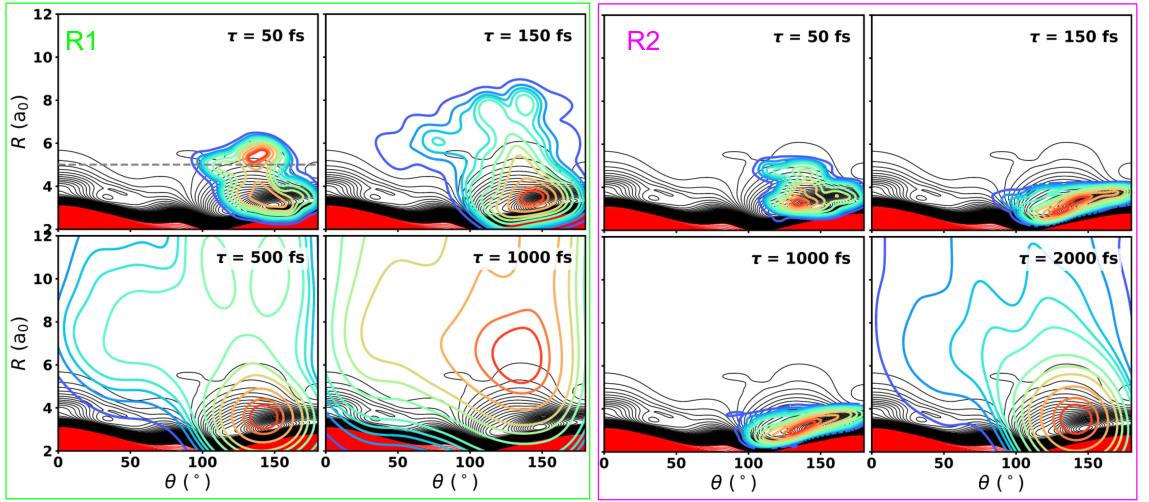
Figure 7 shows the dependence of the 2-dimensional probability distributions on the time delay after synchronization for trajectories contributing to R1 and R2, respectively. In R1, the distribution rapidly moves away from the minimum of the PES and within 1 ps the maximum of the distribution has reached the loose transition state , see Figure 1. In contrast, for R2 remains trapped above the minimum energy geometry of the PES and only starts to move away on the 2 ps time scale. This can also be seen in the lifetime distribution of the trajectories contributing to R1 and R2, shown in Figure S9.
3.3 Phase Space Analysis
After establishing that the QCT simulations provide a qualitatively
correct picture of the TR-CEI experiments, the underlying reaction
dynamics were analyzed in more detail. A prime question concerns the
statisticality of the dynamics, including energy redistribution,
randomization of the dynamics, phase space sampling, ergodicity,
barrier recrossing, and related microscopic behavior. For a phase
space view of the dissociation process, it is useful to generate
Poincaré maps which relate position and momentum (velocity) of the
particles. In the following, three different aspects are analyzed in
more detail: the fraction of available phase space sampled by a
typical trajectory with a given lifetime, the distribution of
residence and recurrence times, and the dependence of Lyapunov
exponents on the lifetimes of neighbouring trajectories.
Analysis of Fractional Area Sampled: As the highly energized,
“hot” parent species [NO2]∤ is generated from a
half-collision NO+O at low collision energy, it is reasonable to
assume that the ensemble of longest-lived trajectories sampling the
NO2 well provide a meaningful rendering of the total available
phase space. Such phase space trajectories are shown in Figure
8. Trajectories were grouped according to their
lifetime. The four rows in Figure 8 correspond to
the lifetime intervals ps, ps, ps,
and ps, respectively. For each
interval, phase space data from a large ensemble of independent
trajectories were accumulated to construct the gray background
distributions. Superimposed on each distribution is one representative
inelastic scattering trajectory from the corresponding lifetime
interval, from which the fractional area explored by an individual
trajectory can be determined. As the lifetime of the highly excited
collision complex increases (large ), the fractional area
covered by a single trajectory progressively increases. A
complementary phase space representation based on the Jacobi
coordinate, , and its conjugate velocity, , is shown in
Figure S10 for representative trajectories from the
same lifetime intervals.

An alternative representation based on the coordinate
further illustrates how
the dissociation dynamics changes with the lifetime of the complex
(Figures S11 and S12). For
short-lived trajectories, rapidly departs from zero
(i.e. equal N-O bond lengths) and adopts either a positive or negative
value, indicating an early selection of the final dissociation
arrangement. As the lifetime increases, the trajectories undergo
increasingly prolonged oscillations around before
separation. Correspondingly, the projections
evolve from a comparatively small number of loops into densely wound
trajectories that repeatedly cross both and
. These repeated crossings reflect large amplitude
motion between configurations in which the two N–O distances are
comparable and indicate that the system progressively loses memory of
its initial arrangement before dissociation. This behavior is
consistent with the broader phase-space sampling observed for the
long-lived trajectories and with the gradual approach to statistical
dynamics.

As shown in Figure 9, the quantity measures the mean fraction of the
total accessible phase space area explored by individual trajectories
within each lifetime interval. The occupied fraction was calculated
from 100 representative trajectories for each process and normalized
to the total accessible region in the corresponding phase-space
projection. For elastic trajectories, the statistics is insufficient
for ps and these data are not reported. The
mean occupied phase space fraction increases with
for the three internal-coordinate projections. Evidently, long-lived
trajectories explore larger portions of the accessible phase space
than short-lived ones: 80 % vs. %. The convergence of the
occupied fractions for longer lifetimes suggests that the dynamics
approaches a more space-filling regime, where trajectories have
sufficient time to visit a larger fraction of the available
configurations before leaving the interaction region.
Analysis of Recurrence Times: A complementary analysis is that
of recurrence times, , see Figure
1. The recurrence time for a single trajectory is
defined as the time interval which a particular degree of freedom
spends between successive crossings of a given target value. Depending
on the lifetime of the energized [NO2]∤ complex, multiple
recurrence (and residence) times occur for a single trajectory. The
set of recurrence times summed over all trajectories with a given
lifetime (or lifetime interval) is the distribution of recurrence
times. Examples are given in Figure S13.
For each lifetime interval, all recurrence (or residence) events extracted from the trajectory ensemble were pooled into a single dataset and represented as histograms. To characterize the short-time behavior of the distributions while minimizing the influence of the long-time tail, the fitting was restricted to fs and fs, respectively. The distributions were fitted by maximum-likelihood estimation using the Gamma probability density function
| (3) |
where is the shape parameter, is the scale
parameter, and is the corresponding rate. To allow
a direct comparison with the histogram counts, the fitted probability
density was rescaled by the number of events included in the fit and
by the histogram bin width. The resulting curves therefore represent
the expected number of events per histogram bin rather than a
normalized probability density.
The recurrence- and residence-time distributions in
Figure S13 reveal two complementary aspects of
the phase space dynamics. The recurrence-time distributions, shown in
Figures S13A/C/E/G quantify the time intervals
between successive returns of a trajectory to a prescribed region or
dividing surface in phase space, analogous to the
intervals illustrated in Figure 1. These distributions
are strongly skewed toward short times and are well described by
gamma-like fits, indicating that once a trajectory enters the
interaction region, repeated returns occur rapidly. The fitted shape
parameters further suggest an approximately memoryless
return process, consistent with efficient local mixing inside the
transient [NO2]∤ collision complex.
In contrast, the residence-time distributions in
Figures S13B/D/F/H describe the duration for
which trajectories remain in the NO2 well before an attempt to
dissociate is made. These distributions are broader and characterized
by larger values than the recurrence-time distributions. The
similarity of the distributions across increasing lifetime intervals
in Figure S13 suggests that long-lived
trajectories are not necessarily associated with a qualitatively
different local return mechanism; rather, their longer lifetimes allow
a larger number of recurrence and residence events before final
dissociation or separation.
The Gamma shape parameters obtained from the recurrence-time and
residence-time distributions exhibit a dependence on the lifetime
interval (Figure S14). The recurrence-time
parameter, , increases for short-lived
complexes and reaches an approximately constant value for – ps. By contrast, the normalized residence-time
parameter, , reaches a maximum
within this lifetime range and subsequently decreases for longer-lived
complexes. Interestingly, this crossover occurs on a timescale
similar to that at which the relative populations of exchange and
inelastic trajectories become approximately stable, as shown in
Figure 2.
Lyapunov Exponents: The Lyapunov exponents, a measure of the
divergence of neighbouring trajectories, were analyzed for
trajectories exhibiting different lifetimes. It should be noted that
Lyapunov exponents provide a measure of dynamical instability and
local chaoticity. Lyapunov exponents are not direct measures of the
“statisticality” of a process. Rather, they provide a complementary
description of the dynamical instability and evolution of the
collision complex. To characterize this instability within the
interaction region, was
defined as the mean Lyapunov exponent evaluated over the lifetime of
the complex for all trajectories belonging to a given lifetime
interval. As shown in Figure S15,
increases rapidly for the
shortest-lived trajectories, from approximately 0.027 fs-1 in the
– ps interval to fs-1 for lifetimes of
2–3 ps. For longer-lived trajectories,
fluctuates in the interval
fs-1. Correspondingly, the characteristic
randomization time, , decreases from fs
for the shortest-lived trajectories to fs at 2–3 ps, after
which it remains within a relatively narrow range of approximately
– fs. This behavior indicates that dynamical instability
develops rapidly during the first few picoseconds, whereas
longer-lived complexes exhibit a broadly similar characteristic
randomization timescale. Interestingly, this transition occurs within
approximately the same lifetime range highlighted by the dashed line
in the inset of Figure 2, beyond which the relative
fractions of inelastic and exchange trajectories approach comparable
values and remain close to . The similar timescales suggest the
emergence of a common long-lived dynamical regime beyond approximately
2–3 ps.
The time evolution of the separation between initially neighboring
trajectories provides a direct illustration of the dynamical
instability quantified by the Lyapunov exponent
(Figure S16). For both representative trajectories,
the quantity increases predominantly within the
shaded lifetime interval, confirming that the strongest divergence
develops when the system samples the interaction region. For the
short-lived trajectory, the separation grows progressively throughout
most of its lifetime, whereas the longer-lived trajectory exhibits a
rapid initial increase followed by saturation well before
dissociation. This saturation does not imply the disappearance of
chaotic dynamics; rather, it reflects the finite extent of the
available phase space region, limiting the accessible separation
between the trajectories. These examples therefore support the use of
the renormalized Lyapunov analysis to characterize local instability
and indicate that most of the dynamical divergence is established
during the early part of the complex lifetime.

Figure 10 combines the recurrence- and
residence-time statistics with the mean Lyapunov exponent to
characterize the progressive randomization of the dynamics. For
ps, increases
rapidly, indicating that successive returns become less broadly
distributed as the complex explores a larger region of phase
space. Over the same range,
and also change markedly,
showing that the local trapping dynamics and the sensitivity to
initial conditions evolve together. Beyond approximately 2-3 ps,
and the Lyapunov exponents vary more
gradually, whereas reaches a
maximum and subsequently decreases. Thus, the dashed line at 2 ps,
corresponding to the same lifetime boundary marked in
Figure 2, indicating the onset of a regime in which
phase space randomization is substantially developed and the dynamical
observables begin to approach more slowly varying dynamical
behavior.
4 Discussion and Conclusion
The present work discussed the dissociation dynamics of energized
[NO2]∤ in the context of recent TR-CEI experiments and
analyzed the phase space dynamics of the unimolecular decomposition
process. Using a validated reactive PES based on an RKHS
representation provides a realistic picture of evolution along the
dissociation coordinate, as evidenced by the strong agreement
between experiment and theory in Figure 6. The two
prominent features in the measured map, namely
the rapidly decaying (R1) and the quasi-stationary (R2) component,
were successfully captured through dynamics simulations which started
from a slow NO+O collision and the synchronized formation of
[NO2]∤. Further analysis associated R1 and R2 with
trajectories having considerably different lifetime distributions in
the [NO2]∤ state before breakup.
For trajectories with lifetimes ps, the
probability for inelastic collisions between NO and O differs from
that of O atom exchange. In other words, [NO2]∤ lifetimes of
ps appear to be too short to fully randomize the internal
energy required to reach the statistically expected 50 / 50 split
between inelastic and reactive collisions, see Figure
2. This observation is consistent with convergence of
the Gamma shape parameter obtained from analysis of the
recurrence time distributions, for which randomization times of 2 to 3
ps are inferred. Finally, analysis of the Lyapunov exponents indicated
that randomization times are 1 ps and longer. Hence, trajectories
corresponding to R1 in Figure 6 are associated with
non-statistical breakup dynamics whereas those in R2 support the
statistical dynamics assumption.
In the present work the internally “hot” ground state triatomic
[NO2]∤ was generated from a slow collision between NOA + OB under imposed energy and angular momentum
constraints. Synchronization of the trajectories provided a
well-defined “time zero” for the unimolecular decay dynamics of
[NO2]∤, thereby enabling the comparison of TR-CEI experiment
with theory. From the trajectory data, a unique time-resolved
observable was constructed: the Coulombic Recoil Energy upon SFI. In
contrast, earlier workArasaki and Takatsuka (2007) projected an initial
wavepacket from the ground state onto the electronically excited state
and propagated it through the conical intersection. After reaching
this crossing, parts of the wavepacket switched to the ground state
whereas the remainder continued on the excited state PES until most of
the population was transferred to the ground state after
fs. From here, dissociation into NO+O was followed in a fashion
analogous to the present work. Differences between the present work
and earlier simulations concern non-adiabatic effects - not included
here since the focus is on [NO2]∤ ground state dynamics
after all non-adiabatic processes are essentially complete - and the
higher quality of the underlying PES(s) in the present work and the
construction of new time-resolved observables.
Time-Resolved Coulomb Explosion Imaging (TR-CEI) is a novel
experimental probe of ground state unimolecular dissociation
dynamics. It provides a direct map of the evolution of the scalar
distance between departing photofragments and is particularly
important at longer ranges: to the best of our knowledge, no other
observable is sensitive to evolution in this large-amplitude region of
unimolecular dynamics. A key assumption of statistical theories of
unimolecular reaction dynamics is that phase space is uniformly filled
on time scales short compared to dissociation. The present results,
however, indicate that the filling of phase space takes time and is
not uniform. The present work argues that the time evolution of as
provided by TR-CEI yields a novel observation of phase space dynamics
and serves as a meaningful route to discerning the parallel
non-statistical and statistical aspects - which each participate here
- of the unimolecular dissociation of NO2.
Data Availability
The codes and data for the present study are available from https://github.com/MMunibas/NN-coulomb upon publication.
Acknowledgment
The authors gratefully acknowledge financial support from the Swiss
National Science Foundation through grants (MM),
(MM), and the University of Basel (MM). A. Stolow and
A. Staudte thank the NSERC Discovery Grant program, NRC QSP Challenge
Program Project QSP-075-01, and the Joint Centre for Extreme Photonics
for financial support. A. Stolow thanks the Canada Research Chairs
program for support.
Supporting Material: Observing Phase Space Evolution During Unimolecular Decay
S1 Details about PESs
In the past a wide range of potential energy surfaces (PESs) for the
reactive O+NO system has been generated and used for various
purposes. For example, the vibrational state-dependent cross sections
have been calculated from dynamics
studies.Caridade and Varandas (2004); Duff et al. (1994); Ramachandran et al. (2000) One
PESDuff et al. (1994) for the 2A′ state used a fit to electronic
structure calculations at the complete active space SCF (CASSCF) level
followed by multireference contracted configuration interaction and a
modified Duijneveldt (11s6p) basis set.Walch and Jaffe (1987) Another PES
was based on 1250 (for the 2A′) and 910 (4A′) CASPT2
calculations and fitted to an analytical function.Sayós et al. (2002) Such
an approach was also used for the 2A′′ state.González et al. (2001)
Complementary, a PESs for the 2A′ state using a diatomics in
molecules (DIM) expansion with the two-body terms based on extended
Hartree-Fock calculations.Varandas (2003) Then, a 2-dimensional
PES with the NO bond length fixed at its equilibrium value of 2.176
a0 was determined at the icMRCI+Q level of theory and a cc-pVQZ and
represented as a cubic spline.Ivanov et al. (2007) This work also
presented a PES for the 2A′′ state. More recently, a double many
body expansion fit to 1700 points at the MRCI/aug-cc-VQZ level of
theory for the 2A′′ state was carried out.Mota et al. (2012) In
addition, quasi classical trajectory (QCT)
calculationsCaridade and Varandas (2004); Castro-Palacio et al. (2014); Bose and Candler (1997); Sayós et al. (2002)
have been reported for the temperature dependent rate for the
N(4S)+O2 NO+O and its reverse reaction using
different PESs. Most recently, two machine learning-based PESs were
reported. One of them used CASPT2 reference data and was represented
as a many body permutationally invariant polynomialVarga and Truhlar (2021) and
the other one used MRCI+Q calculations as the reference method and a
reproducing kernel Hilbert space (RKHS) for representing
them.San Vicente Veliz et al. (2020); Unke and Meuwly (2017)
S2 Figures


The Coulomb repulsion energies for the different reaction channels are
shown in Panels C–E, corresponding to the inelastic, elastic, and
atom-exchange channels, respectively. As in Panels A and B, the
trajectories can be classified into two regimes, R1 and R2. In the R1
regime, the Coulomb energy decays on a timescale of ps,
whereas in the R2 regime it remains largely constant at values greater
than 4 eV during the first 1 ps. The trajectories contributing to the
R1 regime in Panel A originate predominantly from the atom-exchange
channel (Panel C), whereas those contributing to the R2 regime in
Panel A arise predominantly from the inelastic channel (Panel E). Only
approximately of all trajectories are elastic, resulting in the
sparse distribution observed in Panel D.


References
- Time-resolved photoelectron spectroscopy of wavepackets through a conical intersection in no2. J. Chem. Phys. 132 (12). Cited by: §1.
- Quantum wavepacket dynamics for time-resolved photoelectron spectroscopy of the no2 conical intersection. Chem. Phys. 338 (2-3), pp. 175–185. Cited by: §1, §1, Figure 6, §4.
- Unimolecular reaction dynamics: theory and experiments. Vol. 31, Oxford university press. Cited by: §1.
- An improved potential energy surface and multi-temperature quasiclassical trajectory calculations of N + N dissociation reactions. J. Chem. Phys. 143 (5), pp. 054304. Cited by: §2.2.
- Thermal rate constants of the o + n no + o reaction based on the a and a potential-energy surfaces. J. Chem. Phys. 107 (16), pp. 6136–6145. Cited by: §1, §S1.
- Dynamics study of the n(s) + o reaction and its reverse. J. Phys. Chem. A 108 (16), pp. 3556–3564. Cited by: §1, §S1.
- Computational study of collisions between O(P) and NO() at temperatures relevant to the hypersonic flight regime. J. Chem. Phys. 141 (16), pp. 164319. External Links: ISSN 0021-9606 Cited by: §1, §S1.
- Threshold photodissociation dynamics of NO studied by time-resolved cold target recoil ion momentum spectroscopy. J. Chem. Phys. 151 (17), pp. 174301. External Links: Document Cited by: §1.
- Threshold photodissociation dynamics of no studied by time-resolved cold target recoil ion momentum spectroscopy. J. Chem. Phys. 151 (17), pp. 174301. External Links: Document Cited by: §1, Figure 6, §3.2, §3.2.
- Classical dynamics of the n(s) + o (x) → no(x) + o(p) reaction. Geophys. Res. Lett. 21 (18), pp. 2043–2046. External Links: Document, Link Cited by: §1, §S1.
- Capturing roaming molecular fragments in real time. Science 370 (6520), pp. 1072–1077. Cited by: §1.
- Excited state wavepacket dynamics in no probed by strong-field ionization. J. Chem. Phys. 147 (5). Cited by: §1.
- Ab initio, vtst, and qct study of the a potential energy surface of the n(d) + o(x) o(p) + no(x) reaction. J. Chem. Phys. 115 (19), pp. 8838–8851. External Links: Document Cited by: §1, §S1.
- Unimolecular dissociation of NO. I. classical trajectory and statistical calculations on a global potential energy surface. J. Chem. Phys. 111 (2), pp. 619–632. External Links: Document Cited by: §1.
- The monoenergetic unimolecular reaction of expansion-cooled NO: NO product state distributions at excess energies 0–3000 cm. The Journal of Chemical Physics 99, pp. 1093–1102. External Links: Document Cited by: §1.
- Probing the NO NO + O transition state via time resolved unimolecular decomposition. The Journal of Chemical Physics 99, pp. 3420–3435. External Links: Document Cited by: §1.
- Theoretical investigation of exchange and recombination reactions in o(p)+no() collisions. J. Chem. Phys. 126 (5), pp. 054304. External Links: Document Cited by: §1, §S1.
- The photodissociation threshold of no2: precise determination of its energy and density of states. J. Chem. Phys. 105 (3), pp. 1287–1290. Cited by: §1.
- Exchange reactions with activation energy. i. simple barrier potential for (h, h). J. Chem. Phys. 43, pp. 3259–. Cited by: §2.2, §2.2, §2.2.
- The c(p) + no(x) o(p) + cn(x), n(d)/n(s) + co(x) reaction: rates, branching ratios, and final states from 15 k to 20 000 k. J. Chem. Phys. 149 (9), pp. 094305. External Links: Document Cited by: §2.2.
- Accurate reproducing kernel-based potential energy surfaces for the triplet ground states of no and dynamics for the n + no o + n reaction. Phys. Chem. Chem. Phys. 22 (33), pp. 18488–18498. Cited by: §2.1.
- State-specific unimolecular reaction of NO just above the dissociation threshold. J. Chem. Phys. 99 (1), pp. 254–264. External Links: Document Cited by: §1.
- Ab initio-based global double many-body expansion potential energy surface for the first a electronic state of no. J. Phys. Chem. A 116 (11), pp. 3023–3034. External Links: Document Cited by: §1, §S1.
- Vibrational–rotational distributions of no formed from n+o reactive collisions. Chem. Phys. Lett. 332 (5-6), pp. 562–568. External Links: Document, Link Cited by: §1, §S1.
- Fluctuations in the unimolecular decomposition of jet-cooled no: implications for overlapping resonances and the transition state. J. Chem. Phys. 100 (6), pp. 4256–4271. External Links: Document Cited by: Figure S3, Figure S4, §2.2, §3.1.
- Does a dissociating molecule sample the available phase space. J. Phys. Chem. 95 (19), pp. 7124–7127. Cited by: §1.
- Prompt and delayed dissociation of energy-rich larger molecules. J. Phys. Chem. A 102 (50), pp. 10195–10198. Cited by: §1.
- The n(s) + o(x) o(p) + no(x) reaction: thermal and vibrational relaxation rates for the a, a and a states. Phys. Chem. Chem. Phys. 22 (7), pp. 3927–3939. Cited by: §1, §S1, §2.1, §2.2, §2.2, Figure 4, Figure 5, §3.1, §3.2.
- New analytical (a, a) surfaces and theoretical rate constants for the n(s)+o reaction. J. Chem. Phys. 117 (2), pp. 670–679. Cited by: §1, §S1.
- Time-resolved coulomb explosion imaging: a method to measure structure and dynamics of molecular nuclear wave packets. Phys. Rev. A 58 (1), pp. 426. Cited by: §3.2.
- Reactive scattering cross sections iii: quasiclassical and semiclassical methods. In Atom - Molecule Collision Theory, R. B. Bernstein (Ed.), pp. 505–566. Cited by: §2.2, §2.2, §2.2, §2.2.
- Toolkit for the construction of reproducing kernel-based representations of data: application to multidimensional potential energy surfaces. J. Chem. Inf. Model. 57 (8), pp. 1923–1931. Cited by: §1, §S1.
- A realistic multi-sheeted potential energy surface for no(a) from the double many-body expansion method and a novel multiple energy-switching scheme. J. Chem. Phys. 119 (5), pp. 2596–2613. Cited by: §1, §S1.
- Potential energy surface for high-energy n+ n collisions. Phys. Chem. Chem. Phys. 23 (46), pp. 26273–26284. Cited by: §1, §S1.
- The c(p)+ o() co co() + o(d)/o(p) reaction: thermal and vibrational relaxation rates from 15 k to 20000 k. Phys. Chem. Chem. Phys. 23 (19), pp. 11251–11263. Cited by: §2.2.
- Conical-intersection dynamics and ground-state chemistry probed by extreme-ultraviolet time-resolved photoelectron spectroscopy. Nat. Commun. 9 (1), pp. 3162. Cited by: §1.
- Calculated potential surfaces for the reactions: o+n no+n and n+o no+o. J. Chem. Phys. 86 (12), pp. 6946–6956. Cited by: §1, §S1.
- Ultrafast fragmentation dynamics of carbon dioxide trication induced by an intense laser field: transient deformation route vs direct coulomb repulsion. J. Chem. Phys. 162 (11). Cited by: §3.2.