NEMSim: Learning Control-Conditioned Multi-Event Physical Dynamics via Executable Event-Mechanism Priors
Abstract
High-fidelity simulation of control-conditioned multi-event physical systems is computationally expensive, especially across broad control spaces and long trajectories. In these systems, macroscopic evolution emerges from localized discrete events whose intensities and effects depend on process controls and evolving local states, while the available system knowledge is typically expressed as event-attribute descriptions. Purely data-driven surrogates must infer these event effects from limited trajectory coverage, which can hinder generalization to unseen control regimes. Physics-guided methods instead primarily build on equation-level constraints or differentiable solvers rather than discrete event-rule priors. We therefore propose NEMSim (Neural Event-Mechanism Simulator), which compiles predefined event-attribute descriptions into an executable transition structure linking control-dependent event intensities, prior-guided mechanism attribution, and state-dependent responses. To enable evaluation of control-conditioned multi-event dynamics with explicit system knowledge, we construct a 3D KMC-based benchmark pairing high-fidelity trajectories with explicit event rules, standardized splits, and evaluation protocols. Across three settings, NEMSim reduces Avg. RMSE by – relative to the strongest baseline in each setting. It also remains best in the data-efficiency study with training-data fractions down to . Mechanism analyses further show that these gains arise from executable rule integration rather than prior access or architecture alone.
1College of Integrated Circuits, Zhejiang University
2College of Control Science and Engineering, Zhejiang University
{musthave,jj.xie,dni}@zju.edu.cn, liupw@zju.edu.cn

Introduction
High-fidelity simulation is essential for the analysis and design of control-conditioned multi-event physical systems, whose macroscopic states evolve through repeated localized events, event competition, and the accumulation of their effects over time (Bortz et al. 1975; Gillespie 1977; Fichthorn and Weinberg 1991). The intensities and state effects of these events depend jointly on process controls and evolving local states. Generating long trajectories across a broad control space therefore requires repeatedly resolving numerous state-dependent local events, making high-fidelity simulation computationally expensive. This motivates neural surrogates that can predict long-horizon state evolution across varying process controls. We study this problem through Kinetic Monte Carlo (KMC)-based 3D surface morphology simulation, using plasma etching as a representative application (Economou 2000; Marcos et al. 2003).
Purely data-driven surrogates, including sequence models (Shi et al. 2015; Bengio et al. 2015), graph-based simulators (Sanchez-Gonzalez et al. 2020; Pfaff et al. 2021; Brandstetter et al. 2022), and neural operators (Lu et al. 2021; Li et al. 2021; Kovachki et al. 2023), learn control-conditioned state transitions directly from high-fidelity trajectories. For multi-event dynamics, process controls and evolving local states jointly determine event intensities, while dependencies among events shape how their effects combine in each state transition. The resulting control-state-event combinations are difficult to cover with a finite set of expensive trajectories (Li et al. 2024; Brandstetter et al. 2022). This limited coverage makes direct transition learning data-inefficient, weakens generalization to held-out controls, and amplifies error accumulation during long autoregressive rollouts.
Physics-guided learning offers a complementary way to reduce reliance on trajectory coverage by incorporating prior knowledge into learned dynamics. Most existing formulations, however, are designed around equation-level constraints or numerical structures, including governing-equation residuals, conservation laws, known operators, and differentiable solvers (Raissi et al. 2019; Li et al. 2024; Belbute-Peres et al. 2020; Rackauckas et al. 2020; Liu et al. 2024). For control-conditioned multi-event systems, available knowledge often takes a different form: discrete event rules that specify control dependencies, rate and yield relations, event dependencies, and event-mechanism relations. Such rule-level knowledge does not translate naturally into residual-based constraints or differentiable-solver formulations. The central challenge is therefore not merely to impose physical regularization, but to convert discrete event-attribute priors into an executable and learnable transition structure.
The effects of numerous events can be organized through a limited set of mechanism families, while each mechanism may produce different local responses depending on the current state. This event-mechanism organization motivates NEMSim (Neural Event-Mechanism Simulator), a neural simulator for control-conditioned multi-event physical state evolution. NEMSim compiles predefined event rules into an executable event-mechanism transition structure. Given the current state and process controls, it computes event intensities from rule-specified attributes, attributes event effects to shared mechanism families under rule-defined priors, and realizes the resulting mechanism drives through state-dependent response modes. This factorization preserves event-specific control dependence, enables different events to share mechanism-level structure, and retains the expressiveness required for local state-dependent responses. We conduct experiments on a 3D KMC-based benchmark. The results show that executable event-mechanism priors support accurate 100-step rollouts under unseen controls, temporal extrapolation and limited training data.
Overall, the main contributions of this work include:
- •
Problem and method. We formulate the problem of learning control-conditioned multi-event physical dynamics from discrete event-rule priors and introduce NEMSim, which compiles these priors into an executable event-mechanism transition structure.
- •
Benchmark and protocol. We construct a standardized 3D KMC-based benchmark for control-conditioned multi-event dynamics, pairing high-dimensional trajectories with explicit event rules and providing trajectory-level splits and protocols for control interpolation, control extrapolation, temporal extrapolation, data efficiency, and rule robustness.
- •
Evidence. Across 100-step rollouts, NEMSim reduces Avg. RMSE by , , and under control interpolation, control extrapolation, and temporal extrapolation, respectively, relative to the strongest baseline in each setting. It also remains best with only of the training data, while mechanism analyses further show that the gains arise from executable rule integration rather than prior access or architecture alone.
Related Work
Purely Data-Driven Methods. Data-driven physical simulators use different representations to model state evolution. Recurrent models such as ConvLSTM (Shi et al. 2015) and PredRNN (Wang et al. 2017) learn spatiotemporal dependencies from gridded sequences through memory propagation. Graph-based models, including GNS (Sanchez-Gonzalez et al. 2020), MeshGraphNet (Pfaff et al. 2021), and EAGLE (Janny et al. 2023), model particle or mesh interactions through message passing or attention. Neural operators such as DeepONet (Lu et al. 2021), FNO (Li et al. 2021), U-NO (Rahman et al. 2023), and CNO (Raonić et al. 2023) learn mappings between physical fields, while GNOT (Hao et al. 2023) and Transolver (Wu et al. 2024) further use attention to capture long-range dependencies. These methods typically learn direct mappings from observed states and controls to future states.
Physics-Guided Methods. Physics-guided learning embeds prior structure into neural prediction. PINNs and PINOs impose PDE residuals or equation-level operator constraints (Raissi et al. 2019; Li et al. 2024), while differentiable-physics and Universal Differential Equation frameworks embed numerical solvers or known dynamics terms (Belbute-Peres et al. 2020; Rackauckas et al. 2020). Chemical Reaction Neural Networks encode mass-action and Arrhenius kinetics (Ji and Deng 2021), while Mechanistic Neural Networks learn explicit differential-equation representations (Pervez et al. 2024). PRIMME (Yan et al. 2022) encodes local transition constraints for grain growth, while PAPM (Liu et al. 2024) incorporates operating conditions and conservation constraints into process surrogates. These methods primarily express prior knowledge through equations, kinetic laws, solver structures, or regularization, rather than heterogeneous event-rule libraries.
Benchmarks for Physical Learning. PDEBench (Takamoto et al. 2022), APEBench (Koehler et al. 2024), and CFDBench (Luo et al. 2023) standardize learning from PDE and CFD trajectories. A recent phase-field benchmark provides microstructure-evolution trajectories (Rieger et al. 2024). The underlying systems in these benchmarks are primarily specified through governing equations, boundary conditions, geometries, or numerical operators, rather than heterogeneous control-dependent multi-event descriptions.
Method
NEMSim learns control-conditioned multi-event state transitions by compiling an Event Rules Library into an executable event-mechanism transition structure. We first formulate the one-step prediction problem and formalize the Event Rules Library, and then describe the architecture that realizes this factorization.
Problem Setting and Notation
Let denote the system-state space and the process-control space. At transition step , the current state is and the applied process control is . We formulate the task as learning the one-step control-conditioned transition from to . In our benchmark, is represented as a two-channel 3D signed-distance field of the evolving morphology. The control vector contains supply-rate, energy-scale, and incidence-orientation controls.
NEMSim incorporates an Event Rules Library and organizes event effects across a predefined set of mechanism families , where and denote the numbers of event types and mechanism families, respectively. Each event rule is represented as
| (1) |
where , , , , and respectively specify the control bindings, probability relation, yield relation, product-mediated dependencies, and event-mechanism role. The role defines the fixed event-mechanism prior . The rule attributes are further encoded as an event descriptor for subsequent mechanism-attribution and state-response computations. The Event Rules Library provides fixed, system-specific priors that structure the forward transition without event- or mechanism-level supervision. Complete rule definitions, executable attributes, and their instantiation for the benchmark system are provided in the supplementary material (Secs. S3.1, S3.2, and S3.3).
Given fixed structural inputs and , NEMSim learns
| (2) |
where and provide fixed structural priors for the transition, while the neural parameters are learned from state trajectories.
Given , the model is trained using only one-step state-transition supervision:
| (3) |
where denotes the mean squared error over all elements of the normalized state fields.
During long-horizon evaluation, the learned transition is recursively applied from the true initial state under the trajectory-specific control:
| (4) |
The transition combines deterministic rule-derived quantities with learned rule-conditioned corrections and state-dependent responses. Its learnable components are optimized solely through , without intermediate supervision.
Model Architecture
As illustrated in Fig. 1, NEMSim predicts the next state through event-intensity, mechanism-attribution, and state-response compilation. Fig. 2 details the internal computations of the three compilation stages.
State Encoder.
The State Encoder maps the current state to a latent field, a decoder support feature, and a compact state context:
| (5) |
where supports spatial response computation, conditions event and mechanism compilation, and is reused by the decoder.

Event-Mechanism Compiler.
The Event-Mechanism Compiler (EMC) compiles event intensities and event-to-mechanism attribution from the compact state context, process control, and Event Rules Library:
| (6) |
Here, denotes the event-intensity vector, and denotes the event-to-mechanism attribution. Their element-wise product forms the event-mechanism drive , which is passed to the Mechanism Response Compiler.
Event Intensity Compilation. As shown in Fig. 2(1), EIC determines how strongly each event acts under the current state and process control. For each primary event, the control bindings select the event-specific supply, energetic, and directional controls , , and from . The rule-defined base intensity is
| (7) |
The differentiable probability and yield relations and are specified by event rule and instantiated from established physics-based and empirical rate/yield models. Their complete functional forms are provided in the supplementary material (Sec. S3.4).
To account for transition-specific variation not captured by the fixed rules, EIC applies a bounded correction in log-rate space:
| (8) |
where is the rule-conditioned state-control context, predicts the log-rate correction, and bounds its magnitude. The resulting is a nonnegative primary-event intensity with bounded deviation from the rule-defined base.
For product-mediated events, the Product Pool first aggregates the products generated by upstream events and then uses their availability to determine the dependency-driven intensity according to . This represents the pathway from product-generating events to downstream product-consuming events. The final event intensity is , which is passed to MAC. Complete kinetic, bounded-correction, and Product Pool formulations are provided in the supplementary material (Secs. S3.4 and S4.1).
Mechanism Attribution Compilation. EIC determines the strengths of the event effects, while MAC determines how these effects are distributed among the mechanism families. As shown in Fig. 2(2), MAC assigns the compiled event intensities to physical, chemical, and coupled mechanisms.
MAC first combines the fixed event-mechanism prior with how well the event attributes match each mechanism family. This produces the default attribution . The prior specifies the initial mechanism preference, while the default attribution incorporates the event attributes before state-control adaptation.
MAC then bounds the event intensities and computes a rule-based correction :
| (9) |
Here, is the bounded event-intensity signal. Bounding reduces intensity-scale differences before mechanism attribution. uses mechanism-relevant attributes and dependency relations in to produce .
A lightweight context correction further uses the event attributes, compact state context, and process control. The final attribution is
| (10) |
Here, is the bounded attribution correction, scales the context contribution, and limits the overall update. Normalization produces nonnegative attributions that sum to one over . This preserves the rule-defined mechanism preference while allowing the current state and process control to adjust it. Detailed default-attribution, bounded-intensity, and correction formulations are provided in the supplementary material (Secs. S3.5 and S4.2).
Mechanism Response Compiler.
MRC converts the event-mechanism drivers into a latent state increment. As shown in Fig. 2(3), it organizes event-level drivers into mechanism-specific response modes, maps them to bounded amplitudes, and combines them with state-dependent spatial response fields.
Event-to-Modes Signature. Events routed through the same mechanism family can induce different response modes. MRC maps each event descriptor to a distribution over the response modes of every mechanism family:
| (11) |
Here, produces mode-assignment logits, and specifies how the driver of event is distributed across response modes under mechanism . The softmax produces nonnegative weights that sum to one over , retaining event-specific response preferences within shared mechanisms.
Mechanism-Mode Drive. The event-mechanism drivers are aggregated into mechanism-mode drives:
| (12) |
Here, represents the aggregated drive of response mode under mechanism . This aggregation compresses the event-level drivers into a compact mechanism-mode representation.
Saturating Response Law. To model finite response capacity under state constraints and event competition, MRC predicts a state-control gate and a saturating mode amplitude:
| (13) |
Here, predicts the realizability gate, is the response capacity, and is the saturation scale. The resulting is a bounded, state-control-dependent amplitude for mechanism mode .
Spatial Response Composition. Each mode generates a normalized spatial response field from the current latent state:
| (14) |
where determines the state-dependent response pattern. The latent increment is then
| (15) |
where is the number of response modes per mechanism. Thus, determines which modes are driven, determines their realized amplitudes, and determines their spatial response patterns. Event-descriptor construction, network parameterization, field normalization, and tensor dimensions are provided in the supplementary material (Secs. S3.2 and S4.3).
State Increment Decoder.
The decoder maps the mechanism-induced latent response back to the state space through a residual transition:
| (16) |
Here, provides support features, while the residual formulation focuses prediction on transition-induced changes.
Experiments
We evaluate NEMSim on a 3D KMC-based benchmark under three 100-step rollout settings: control interpolation, control extrapolation and temporal extrapolation. We further examine prior-access and structure controls, training-data efficiency, robustness to perturbed event rules, mechanism-aligned counterfactual analysis, and component ablations.
Experimental Setup
Benchmark and protocol. The benchmark trajectories are generated using a reference particle-based Monte Carlo feature-profile simulator. The dataset contains 500 trajectories, each comprising 101 two-channel 3D signed-distance fields and 100 consecutive transitions on a grid. Each supervised sample is represented as , where contains the process controls and remains fixed within each trajectory while varying across trajectories. All splits are constructed at the trajectory level, with no transition from the same trajectory shared across training, validation, and test sets. The Event Rules Library is fixed before dataset splitting and contains no trajectory-specific event realizations, target states, split information, or evaluation statistics. Models are trained with one-step state-transition supervision and evaluated through 100-step autoregressive rollouts without ground-truth correction. Complete benchmark construction, evaluation protocol, and Event Rules Library details are provided in the supplementary material (Secs. S2.1–S2.5 and S3.1).
Evaluation Settings. We evaluate all models under three 100-step rollout settings. Control-ID measures generalization to unseen control configurations within the training control domain. Control-OOD evaluates extrapolation along the Ar+ and Cl+ incident-flux dimensions selected through final-state sensitivity analysis, with their boundary regions held out from training. We consider OOD-Ar+, OOD-Cl+, and OOD-Joint, where the latter holds out boundary regions along both control dimensions. Temporal Extrapolation restricts training to transitions from only the first or of each training trajectory and evaluates full-horizon prediction on trajectory-disjoint test cases. Detailed sensitivity analysis and split construction are provided in the supplementary material (Sec. S2.5).
Baselines. We compare NEMSim with five representative spatiotemporal and neural-operator baselines adapted to 3D state-transition prediction: ConvLSTM (Shi et al. 2015), FNO (Li et al. 2021), U-NO (Rahman et al. 2023), CNO (Raonić et al. 2023), and DeepONet (Lu et al. 2021). The standard baselines receive the same state-control inputs and use identical trajectory-level splits, one-step supervision, and autoregressive evaluation protocols. To isolate the effect of prior access, we further construct CNO+Prior and DeepONet+Prior, which receive deterministic RuleFeat representations derived from the same Event Rules Library used by NEMSim. Architectural adaptations, RuleFeat construction, and training details are provided in the supplementary material (Secs. S5.3 and S6).
Evaluation Metrics. We report average rollout RMSE (Avg. RMSE), final-step RMSE (Final RMSE), final-step Chamfer distance (CD), and the number of trainable parameters (Params.). Avg. RMSE is the mean of the per-step RMSE values over all 100 rollout steps, whereas Final RMSE measures the field error at the final step. CD is computed between the surfaces extracted from the predicted and ground-truth final-step fields and measures final-surface discrepancy. Params. is reported in millions to compare model compactness. Detailed metric definitions, channel aggregation, and surface-extraction settings are provided in the supplementary material (Sec. S2.5).
| Method | Control-ID | OOD-Joint | Vis-50% | Params. (M) | ||||||
|---|---|---|---|---|---|---|---|---|---|---|
| Avg. RMSE | Final RMSE | CD | Avg. RMSE | Final RMSE | CD | Avg. RMSE | Final RMSE | CD | ||
| ConvLSTM | 0.2730 | 0.4557 | 3.847 | 0.3657 | 0.6513 | 3.360 | 0.7117 | 0.8835 | 3.596 | 0.634 |
| FNO | 0.5263 | 0.7510 | 3.838 | 0.4318 | 0.5639 | 2.865 | 0.4747 | 0.5995 | 3.398 | 1.358 |
| U-NO | 0.4526 | 0.5403 | 3.849 | 0.5673 | 0.7861 | 3.567 | 0.4131 | 0.5069 | 3.515 | 2.432 |
| CNO | 0.1841 | 0.3027 | 2.005 | 0.2552 | 0.4078 | 2.282 | 0.1041 | 0.2275 | 1.307 | 1.734 |
| DeepONet | 0.0365 | 0.0842 | 0.987 | 0.1243 | 0.2120 | 1.122 | 0.1207 | 0.2004 | 1.202 | 1.720 |
| CNO+Prior | – | – | – | 0.1992 | 0.3513 | 1.555 | 0.0880 | 0.2051 | 1.253 | 1.751 |
| DeepONet+Prior | – | – | – | 0.1165 | 0.2161 | 1.088 | 0.1300 | 0.1682 | 1.026 | 1.736 |
| NEMSim (ours) | 0.0134 | 0.0316 | 0.519 | 0.0511 | 0.1141 | 0.851 | 0.0195 | 0.0659 | 0.621 | 0.253 |
Main Results
Performance Comparison.
Table 1 reports the 100-step autoregressive rollout performance. Our observations from the results are as follows:
Firstly, NEMSim achieves the most accurate 100-step rollouts under unseen in-distribution control configurations. Compared with DeepONet, it reduces Avg. RMSE, Final RMSE, and CD by , , and , respectively, while using only M trainable parameters. These results demonstrate consistent improvements in both rollout-wide field prediction and final-state geometry.
Secondly, NEMSim maintains its performance advantage under both control and temporal extrapolation. Relative to the strongest standard baseline in each setting, it reduces Avg. RMSE by under OOD-Joint and by under Vis-50%. Consistent reductions in Avg. RMSE, Final RMSE, and CD demonstrate improved generalization to held-out control regions and later evolution stages.
Thirdly, feature-level access to information derived from the same Event Rules Library does not close the performance gap. As shown in Table 1, NEMSim reduces Avg. RMSE relative to the strongest prior-augmented baseline by under OOD-Joint and by under Vis-50%. These results show that the gains cannot be attributed to feature-level prior access alone, but arise from operationalizing the rules through the executable event-mechanism transition structure.
Visualization.
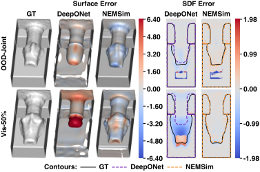
As shown in Fig. 3, NEMSim maintains lower stepwise RMSE than CNO and DeepONet under both OOD-Joint and Vis-50%. Its advantage remains pronounced after the Vis-50% rollout enters the temporally extrapolative stage, indicating reduced long-horizon error accumulation. Fig. 4 further shows that DeepONet produces substantial surface deviations and contour misalignment near the trench bottom and sidewalls, where rollout errors accumulate most visibly. In contrast, NEMSim better preserves these challenging regions, with final surfaces and SDF contours more closely aligned with the ground truth.
Data Efficiency
To assess data efficiency, we train NEMSim, DeepONet, and DeepONet+Prior using , , , and of the training trajectories under the same OOD-Joint protocol. As shown in Fig. 5, NEMSim achieves the lowest Avg. RMSE and final-step CD at every data fraction. With only of the training trajectories, its Avg. RMSE remains below and is lower than both DeepONet variants trained with the complete training partition. The sustained advantage over DeepONet+Prior shows that feature-level prior access alone cannot explain the data-efficiency gains, supporting the role of the executable event-mechanism transition structure.
Mechanism Analysis
Prior Ablation and Robustness.
Table 2 examines whether rule semantics provide predictive value beyond the event-mechanism architecture and how performance changes under imperfect prior information. Structure-only replaces all rule semantics with fixed anonymous embeddings while retaining the same model topology and parameter capacity. Mechanism Shuffle randomly selects of the events and reassigns their mechanism priors to different mechanism families; Event Drop randomly selects of the event rules and disables them by setting their intensities to zero; and Rate/Yield Noise independently scales each positive rate and yield parameter by a factor sampled from .
The full model outperforms Structure-only under the same model topology and parameter capacity, showing that rule semantics provide predictive value beyond architectural structure alone. All ablated and perturbed variants degrade performance relative to the full model, confirming that the encoded rule knowledge is functionally used. The perturbed variants nevertheless retain nontrivial predictive performance, indicating partial tolerance to imperfect rule information.
| Variant | Avg. RMSE | Final RMSE | CD |
|---|---|---|---|
| NEMSim (Full) | 0.0511 | 0.1141 | 0.851 |
| Structure-only | 0.0684 | 0.1525 | 0.944 |
| Mechanism Shuffle | 0.0683 | 0.1497 | 0.896 |
| Event Drop | 0.0892 | 0.2167 | 0.892 |
| Rate/Yield Noise | 0.0944 | 0.1812 | 1.117 |

Mechanism-Aligned Response Analysis.
We fix the input state and counterfactually perturb the Cl+ and neutral Cl flux controls relative to their nominal values. Each flux is independently scaled to or , covering four single-control and four joint perturbations, while the unperturbed setting serves as the reference. We then measure the resulting changes in the learned mechanism responses and predicted material removal.
As shown in Fig. 6(a), the perturbations produce control-role-specific and directionally consistent responses. Increasing the Cl+ flux primarily strengthens the physical and coupled responses, consistent with enhanced ion bombardment and ion-assisted removal, whereas increasing the neutral Cl flux selectively strengthens the chemical response, consistent with enhanced surface-chemical activity. Decreasing either flux produces the opposite trend, while joint perturbations combine the two response patterns. Fig. 6(b) further shows that, under Cl+-related interventions, stronger coupled responses correspond to greater material removal, whereas neutral-Cl-only interventions exhibit weaker immediate correlations, as expected from their primarily chemical role. Together, these counterfactual results provide evidence that NEMSim learns control-specific internal responses that are physically aligned and reflected in state changes, marking a concrete step toward interpretable neural simulation.
Ablation Studies
We individually remove EIC, MAC, and MRC while keeping all other architectural and training settings unchanged. Removing any single component consistently degrades Avg. RMSE, Final RMSE, and CD across all three settings, increasing Avg. RMSE by –, with the largest absolute degradation under OOD-Joint. These results show that the complete EIC-MAC-MRC pathway is functionally necessary for the observed rollout performance, particularly under extrapolation. Complete results are provided in the supplementary material (Sec. S5.7).
Conclusion and Limitations
We proposed NEMSim, a neural simulator that compiles predefined event-attribute descriptions into an executable event–mechanism transition structure for control-conditioned multi-event physical dynamics. By organizing event intensity, mechanism routing, and state-dependent response composition, NEMSim reduces Avg. RMSE by – across three 100-step rollout settings and remains superior with only of the training data. Prior-controlled comparisons, rule perturbations, ablations, and mechanism-aligned analyses further support the benefit of executable rule integration beyond prior access or architectural structure alone.
The current evaluation is limited to one 3D KMC-based plasma-etching benchmark, reflecting the scarcity of public benchmarks for control-conditioned multi-event physical dynamics. NEMSim also produces deterministic rollouts and assumes predefined event-attribute descriptions. Future work will broaden the evaluation, develop probabilistic rollouts for uncertainty estimation, and support data-driven event discovery and rule refinement.
References
- Combining differentiable PDE solvers and graph neural networks for fluid flow prediction. In Proceedings of the 37th International Conference on Machine Learning, Proceedings of Machine Learning Research, Vol. 119, pp. 2402–2411. Cited by: Introduction, Related Work.
- Scheduled sampling for sequence prediction with recurrent neural networks. In Advances in Neural Information Processing Systems, Vol. 28, pp. 1171–1179. Cited by: Introduction.
- A new algorithm for monte carlo simulation of ising spin systems. Journal of Computational Physics 17 (1), pp. 10–18. External Links: Document Cited by: Introduction.
- Message passing neural PDE solvers. In International Conference on Learning Representations, Cited by: Introduction.
- Modeling and simulation of plasma etching reactors for microelectronics. Thin Solid Films 365 (2), pp. 348–367. External Links: Document Cited by: §S1.1, Introduction.
- Theoretical foundations of dynamical monte carlo simulations. The Journal of Chemical Physics 95 (2), pp. 1090–1096. External Links: Document Cited by: Introduction.
- Exact stochastic simulation of coupled chemical reactions. The Journal of Physical Chemistry 81 (25), pp. 2340–2361. External Links: Document Cited by: Introduction.
- GNOT: a general neural operator transformer for operator learning. In Proceedings of the 40th International Conference on Machine Learning, Proceedings of Machine Learning Research, Vol. 202, pp. 12556–12569. Cited by: Related Work.
- Nano-scale feature profile modeling of plasma material processing. Ph.D. dissertation, University of Michigan, Ann Arbor, Michigan. Cited by: §S2.1, §S3.1, §S3.3, §S3.3, §S3.4, §S3.4, §S3.5.
- EAGLE: large-scale learning of turbulent fluid dynamics with mesh transformers. In International Conference on Learning Representations, Cited by: Related Work.
- Autonomous discovery of unknown reaction pathways from data by chemical reaction neural network. The Journal of Physical Chemistry A 125 (4), pp. 1082–1092. External Links: Document Cited by: Related Work.
- APEBench: a benchmark for autoregressive neural emulators of PDEs. In Advances in Neural Information Processing Systems, Vol. 37, pp. 120252–120310. External Links: Document Cited by: Related Work.
- Neural operator: learning maps between function spaces with applications to PDEs. Journal of Machine Learning Research 24 (89), pp. 1–97. Cited by: Introduction.
- Fourier neural operator for parametric partial differential equations. In International Conference on Learning Representations, Cited by: Introduction, Related Work, Experimental Setup.
- Physics-informed neural operator for learning partial differential equations. ACM/IMS Journal of Data Science 1 (3), pp. 1–27. External Links: Document Cited by: Introduction, Introduction, Related Work.
- PAPM: a physics-aware proxy model for process systems. In Proceedings of the 41st International Conference on Machine Learning, Proceedings of Machine Learning Research, Vol. 235, pp. 31080–31105. Cited by: Introduction, Related Work.
- Learning nonlinear operators via DeepONet based on the universal approximation theorem of operators. Nature Machine Intelligence 3 (3), pp. 218–229. External Links: Document Cited by: Introduction, Related Work, Experimental Setup.
- CFDBench: a large-scale benchmark for machine learning methods in fluid dynamics. External Links: 2310.05963, Document, Link Cited by: Related Work.
- Monte carlo simulation method for etching of deep trenches in Si by a SF/O plasma mixture. Journal of Vacuum Science & Technology A 21 (1), pp. 87–95. External Links: Document Cited by: §S1.1, Introduction.
- Mechanistic neural networks for scientific machine learning. In Proceedings of the 41st International Conference on Machine Learning, Proceedings of Machine Learning Research, Vol. 235, pp. 40484–40501. Cited by: Related Work.
- Learning mesh-based simulation with graph networks. In International Conference on Learning Representations, Cited by: Introduction, Related Work.
- Universal differential equations for scientific machine learning. External Links: 2001.04385, Document, Link Cited by: Introduction, Related Work.
- U-NO: U-shaped neural operators. Transactions on Machine Learning Research. Cited by: Related Work, Experimental Setup.
- Physics-informed neural networks: a deep learning framework for solving forward and inverse problems involving nonlinear partial differential equations. Journal of Computational Physics 378, pp. 686–707. External Links: Document Cited by: Introduction, Related Work.
- Convolutional neural operators for robust and accurate learning of PDEs. In Advances in Neural Information Processing Systems, Vol. 36, pp. 77187–77200. External Links: Document, Link Cited by: Related Work, Experimental Setup.
- Setting the standard for machine learning in phase field prediction: a benchmark dataset and baseline metrics. Scientific Data 11, pp. 1275. External Links: Document Cited by: Related Work.
- Learning to simulate complex physics with graph networks. In Proceedings of the 37th International Conference on Machine Learning, Proceedings of Machine Learning Research, Vol. 119, pp. 8459–8468. Cited by: Introduction, Related Work.
- Convolutional LSTM network: a machine learning approach for precipitation nowcasting. In Advances in Neural Information Processing Systems, Vol. 28, pp. 802–810. Cited by: Introduction, Related Work, Experimental Setup.
- PDEBench: an extensive benchmark for scientific machine learning. In Advances in Neural Information Processing Systems, Vol. 35, pp. 1596–1611. Cited by: Related Work.
- PredRNN: recurrent neural networks for predictive learning using spatiotemporal LSTMs. In Advances in Neural Information Processing Systems, Vol. 30, pp. 879–888. Cited by: Related Work.
- Transolver: a fast transformer solver for PDEs on general geometries. In Proceedings of the 41st International Conference on Machine Learning, Proceedings of Machine Learning Research, Vol. 235, pp. 53681–53705. Cited by: Related Work.
- A novel physics-regularized interpretable machine learning model for grain growth. Materials & Design 222, pp. 111032. External Links: Document Cited by: Related Work.
- Investigation of feature orientation and consequences of ion tilting during plasma etching with a three-dimensional feature profile simulator. Journal of Vacuum Science & Technology A 35 (2), pp. 021303. External Links: Document Cited by: §S2.1, §S3.1, §S3.1, §S3.3, §S3.3, §S3.4, §S3.4, §S3.5.
Supplementary Material
S1 Physical-System Background
S1.1 Plasma Etching as a Controlled Multi-Event System
Plasma etching is a surface-processing technique in which a plasma supplies ions, neutral reactive species, and electrons to an evolving material surface. External operating conditions regulate the particle supply, energy distribution, and incidence characteristics of these species, thereby controlling how strongly different surface processes are activated (Economou 2000; Marcos et al. 2003). In the benchmark considered in this work, these conditions are represented by process-control variables associated with supply rate, energy scale, and incidence orientation.
Surface evolution results from numerous localized events, including adsorption, desorption, charging, physical sputtering, chemical reaction, ion-assisted reaction, diffusion, and redeposition. The occurrence and effect of each event depend on both the applied controls and the local surface state, such as material composition, site availability, and surface geometry. Moreover, events can compete for the same local sites or interact through assistance and product-mediated dependencies. For example, energetic ions can directly induce physical removal or assist chemical reactions, while reaction products generated upstream may later contribute to redeposition.
Although each event acts locally, repeated event occurrence, competition, and coupling accumulate over time to produce macroscopic 3D morphology evolution. Plasma etching therefore provides a representative control-conditioned multi-event system in which control changes alter not only the magnitude of state updates, but also the relative strengths and interactions of different event pathways. This structure motivates a surrogate model that explicitly organizes the learned transition through event intensity, mechanism attribution, and state-dependent response composition.
S1.2 Particle-Based Monte Carlo Surface-Evolution Simulation
The high-fidelity trajectories are generated using a self-developed particle-based Monte Carlo feature-profile simulator, where surface evolution emerges from repeated stochastic interactions between incident particles and the evolving surface configuration.
Let denote the microscopic surface configuration and denote the applied process controls. At each simulation step, incident particles are sampled according to the control-dependent distributions determined by , including particle flux, energy distribution, and incident-angle distribution. Each sampled particle is transported toward the current surface and interacts with local surface sites according to predefined event rules.
For an incident particle interacting with local surface state , the possible outcomes are determined by the corresponding event attributes:
| (S1) |
where contains the event-specific attributes, including rate-related parameters, yield relations, dependency information, and event-response characteristics. The realized interaction may remove surface materials, generate reactive species, modify local composition, or change neighboring-site availability.
After each microscopic interaction, the surface configuration is updated:
| (S2) |
Because each local interaction modifies the evolving surface state, subsequent particle trajectories and reaction probabilities depend on the updated configuration, resulting in state-dependent event competition and coupling.
A macroscopic morphology state is recorded after a predefined number of particle interactions:
| (S3) |
where converts the microscopic surface configuration into the multi-channel 3D signed-distance fields used by the learning models.
Each transition therefore summarizes the accumulated effects of numerous localized particle-surface interactions rather than a single event realization. Repeated simulation generates high-dimensional morphology trajectories under different control conditions.
Although the simulator explicitly executes microscopic particle interactions, the learning models are not provided with particle trajectories, event locations, realized event identities, microscopic states, or intermediate simulation variables. The Event Rules Library only provides fixed event-attribute descriptions that define possible event categories and their structural relations.
S1.3 Localized Events and Mechanism Families
The simulated surface evolves through a catalog of localized events, each of which modifies a site or a small neighborhood of the current microscopic configuration. Representative events include adsorption, desorption, charging, physical sputtering, chemical reaction, ion-assisted chemical removal, diffusion, and product redeposition. An event is admissible only when its local prerequisites are satisfied, such as the presence of a removable material, an available adsorption site, a required reactant, or a compatible neighboring configuration. Its propensity and local effect are further modulated by the applied process controls and the current surface state.
The event catalog describes what local transition can occur, whereas the mechanism taxonomy describes through which underlying effect the event changes the system. We group the event effects into three mechanism families,
| (S4) |
The physical family represents effects dominated by momentum or energy transfer, incidence geometry, and charged-particle interactions. Typical examples include direct physical sputtering and control-dependent ion-impact responses. The chemical family represents adsorption, surface reaction, desorption, and other transformations governed primarily by reactive-species availability and local chemical state. The coupled family represents processes that require interactions between physical and chemical factors, such as ion-assisted reactions, chemically enhanced sputtering, and product-mediated dependencies.
Event types and mechanism families are not related by a one-to-one assignment. A single event may act through more than one mechanism, while different events may share the same underlying mechanism. For example, an ion-assisted removal event can contain both a chemical contribution associated with surface reaction and a coupled contribution associated with energetic ion assistance. Conversely, several distinct ion-induced events may share a physical energy-transfer mechanism while differing in their rate parameters, products, or local response patterns. This many-to-few organization separates event-specific driving strengths from reusable mechanism-level effects.
For each event rule , the Event Rules Library therefore specifies a prior event–mechanism relation
| (S5) |
where indicates whether and to what extent event is supported by mechanism family . These priors are constructed from the predefined event attributes, including particle type, energetic or directional dependence, reaction role, product dependence, and ion-assistance flags. They are fixed before model training and encode structural support rather than event-occurrence labels or dynamically observed mechanism targets.
The separation between localized events and shared mechanism families is important for control-conditioned morphology evolution. External controls first alter which events are activated and how strongly they occur, while the resulting event effects are expressed through a smaller set of physical, chemical, and coupled response pathways. Their repeated local execution and competition ultimately produce the observed macroscopic 3D state transition.
S2 Benchmark Construction
We construct a benchmark for learning control-conditioned 3D multi-event physical state transitions from high-fidelity reference trajectories. The benchmark targets a setting that is not explicitly covered by existing physical-learning resources: high-dimensional morphology evolution produced by the accumulation and interaction of localized discrete events under externally varying process controls. It is designed not merely as a collection of simulated trajectories, but as an integrated evaluation resource combining state-transition data, process-control metadata, a machine-readable Event Rules Library, predefined data splits, and standardized long-horizon rollout protocols.
The current benchmark instantiation contains 500 trajectories, each comprising 100 transition steps on a three-dimensional grid. Each transition is represented by
| (S6) |
where and are consecutive morphology states and contains the process controls applied during the transition. The Event Rules Library is shared across trajectories and provides fixed system-level metadata rather than trajectory-specific event-occurrence or mechanism labels.
The benchmark defines three complementary evaluation regimes. Control-ID measures interpolation to unseen control configurations within the training control domain; Control-OOD measures generalization to control regions explicitly excluded from training; and Temporal Extrapolation measures whether a one-step transition learned from early trajectory stages can be recursively applied to later unseen stages. All evaluation settings use trajectory-level separation and 100-step autoregressive rollout without ground-truth state correction.
The following subsections describe the reference simulator and physical configuration, trajectory-generation and control-sampling procedure, state and control representations, dataset statistics and quality-control checks, split and evaluation protocols, and the planned release package. The detailed event catalog, kinetic parameters, dependency relations, and mechanism-family priors are documented separately in Sec. S3.
S2.1 High-Fidelity Simulator and Physical Configuration
Reference Simulator and Modeling Scope. The reference trajectories are generated using a three-dimensional particle-based Monte Carlo feature-profile simulator for chlorine-based plasma etching. The simulator resolves individual particle injection and transport, stochastic particle–surface interactions, local multi-species material updates, secondary-product transport, and three-dimensional morphology evolution. Local material changes accumulated from particle interactions are transferred to a level-set solver, which advances the macroscopic Si and resist interfaces.
The simulator serves as the high-fidelity reference relative to the learned surrogate. It should not be interpreted as experimental ground truth or as an exact continuous-time kinetic Monte Carlo solver. In particular, the implementation does not construct a global event-propensity table, sample events according to normalized reaction rates, or advance time using a Gillespie or residence-time increment. Instead, its basic stochastic unit is an incident particle that is propagated through the current geometry and locally interacts with the first accessible surface. The reaction classes and kinetic parameterization are consistent with established Monte Carlo feature-profile models for chlorine-based plasma etching (Huard 2018; Zhang et al. 2017), while the benchmark trajectories follow the implemented simulator configuration described below.
Simulator Availability. The reference simulator is an in-house implementation developed for industrial research collaboration and is subject to confidentiality restrictions. Its complete source code and selected engineering details therefore cannot be publicly released. We disclose the physical configuration, particle-sampling and transport procedure, stochastic surface-interaction process, morphology-update scheme, snapshot cadence, and output representation required to understand the scope and construction of the benchmark. The simulator is used only for offline generation of the fixed reference trajectories and is unavailable to all learning methods during training and evaluation. To support reproducible machine-learning evaluation, the benchmark release will include the generated trajectories, process controls, preprocessing code, data-split manifests, evaluation metrics, baseline configurations, and model implementations.
Physical Domain and Initial Geometry. The simulator maintains a multi-species voxel domain of size
| (S7) |
with array axes corresponding to . A nominal isotropic voxel spacing of is used for the geometric scale and flux-to-particle conversion, giving a nominal physical extent of
| (S8) |
The level-set solver itself operates in lattice coordinates with unit numerical spacing; therefore, reported signed distances are converted and normalized at the representation stage rather than interpreted directly as physical distances in nanometers.
All benchmark cases use the same deterministic initial geometry. The lower voxel layers are initialized as bulk Si. A voxel resist layer is placed above the substrate, occupying , except for a centered cylindrical opening of radius voxels. The uppermost five voxel layers form an initially empty incident region. The nominal substrate thickness, resist thickness, and opening diameter are therefore , , and , respectively.
The lateral boundaries are periodic: a particle leaving the domain in or is wrapped to the opposite side. The vertical boundary is open, and particles leaving through either end of the axis are terminated. A voxel is considered surface-exposed when it contains non-vacuum material and at least one of its six axis-aligned neighbors is vacuum. Local surface normals are estimated from the surrounding material configuration and are used for incidence-angle evaluation, reflection, product emission, and morphology updates.
| Configuration | Implemented value | Interpretation |
|---|---|---|
| Native material domain | Multi-species voxel domain in ordering. | |
| Nominal voxel spacing | Used for geometric scale and flux-to-particle conversion; level-set evolution uses lattice units. | |
| Initial Si region | Bulk silicon substrate with nominal thickness . | |
| Initial resist region | Resist layer with a centered cylindrical opening. | |
| Opening radius | voxels | Nominal radius and diameter . |
| Incident region | Initially empty region above the resist surface. | |
| Particle boundaries | Periodic in and ; open in | Lateral escape is wrapped; vertical escape terminates the particle trajectory. |
| Surface definition | Six-neighbor exposure | A non-vacuum voxel is surface exposed when an axis-aligned neighbor is vacuum. |
| Primary species | Cl, Cl+, Cl, Ar+ | Species are sampled according to control-dependent incident fluxes. |
| Native saved fields | Separate padded mask and Si level-set fields. The model-compatible representation is described in Sec. S2.3. |
Particle Injection and Transport. The primary incident species are Cl, Cl+, Cl, and Ar+. For a given set of process controls, the four incident fluxes are converted into integer particle rates using the top-surface area and a fixed scaling factor. Each primary particle is then sampled from the normalized species-rate distribution.
Particles are launched from the upper boundary at
| (S9) |
with and sampled uniformly over the complete top plane. For incident species , the polar direction follows a cosine-power distribution
| (S10) |
where the exponent is supplied by the process controls. The azimuthal angle is sampled uniformly over . Larger values of produce more narrowly directed incidence around the vertical direction.
The energy of each ion is sampled from a species-specific Gaussian distribution,
| (S11) |
where the mean and standard deviation are determined by the current controls. Neutral Cl particles use a fixed incident energy of .
After initialization, each particle is propagated stepwise in continuous coordinates along its sampled direction. Periodic wrapping is applied in the two lateral directions, and a particle is terminated if it escapes through the open vertical boundary. The implementation limits each particle trajectory to at most propagation steps.
Local Stochastic Surface Interactions. Each voxel stores amounts of multiple local species rather than a single material label. The represented surface states include Si, progressively chlorinated SiClx states, resist, and vacuum. When a particle reaches a surface voxel, a target species is sampled from the local voxel contents. The simulator then evaluates the reaction channels applicable to the projectile–target pair using the configured probability, energy-threshold, angular, and yield models.
Neutral Cl interactions include progressive surface chlorination and lower-probability abstraction or removal branches. Ion-induced interactions include direct physical sputtering, chemically enhanced removal of chlorinated surface species, and resist erosion. For the Cl+–SiCl pair, the implementation explicitly constructs competing physical and chemical channels. When their total probability is below one, the remaining probability corresponds to a non-reactive outcome; otherwise, the two channels are selected according to their normalized relative probabilities. The current implementation uses a single applicable reaction channel for the other projectile–target cases. The complete benchmark event catalog and kinetic parameters are reported in Sec. S3.
Reaction yields are converted into discrete material-removal counts through stochastic sampling. A successful event modifies the local species amounts and can remove material, change its chlorination state, or generate secondary products. If no reaction occurs, an ion undergoes specular reflection with an energy reduction determined by the projectile–target mass relation. Non-reactive neutral particles and secondary products undergo diffuse reflection.
Explicit Secondary-Product Transport. Selected ion-induced removal events generate volatile or redepositable SiCl, SiCl2, and SiCl3 products. Unlike the reduced Product Pool used inside the neural compiler, these products are explicitly represented as secondary particles in the reference simulator. Each generated product is assigned an energy of , zero charge, and an outward direction sampled from a cosine-weighted hemisphere around the local surface normal.
Generated products are placed in a first-in–first-out queue and propagated using the same particle-transport procedure as the primary particles. Upon reaching a supported solid surface, a product deposits with probability
| (S12) |
A product that does not deposit undergoes diffuse reflection and continues to be tracked. The simulator therefore includes explicit secondary-product transport with simplified sticking chemistry rather than a spatially homogeneous redeposition source.
Flux-Triggered Morphology Evolution. Particle interactions first update the local multi-species voxel state. The accumulated material changes are subsequently converted into narrow-band velocity fields for separate Si and mask level sets. After a flux-derived number of incident ions has been processed, both level sets are advanced by one macro step of
| (S13) |
Velocity extension, local smoothing, and level-set reinitialization are applied during this update.
The macro-time variable is calibrated from the incident ion flux rather than sampled from microscopic reaction propensities. Specifically, one macro step is triggered after processing approximately
| (S14) |
incident ions, where is the total control-dependent ion rate. Because neutral particles are interleaved with ions through stochastic species sampling, the total number of primary particles and successful local reactions within a macro step varies across process controls and stochastic realizations.
Saved Reference States and Task Boundary. The simulator is advanced from macro-time to and records a state every . Each trajectory therefore contains
| (S15) |
giving 101 saved states and 100 consecutive benchmark transitions. Each saved transition spans five level-set macro steps and aggregates many incident particles, stochastic surface interactions, material updates, and secondary-product trajectories. It is therefore a coarse-grained morphology transition rather than a single microscopic event.
The simulator natively stores separate padded Si and mask level-set fields at resolution. It does not provide microscopic event identities, event locations, particle histories, reaction outcomes, or internal random seeds as learning targets. The transformation of these native fields into the two-channel, model-compatible benchmark state representation is described in Sec. S2.3.
S2.2 Trajectory Generation and Control-Space Sampling
Process-Control Parameterization. Each simulator trajectory is conditioned on a 14-dimensional process-control vector,
| (S16) |
which controls the incident particle supply, directional distribution, and ion-energy distribution. The flux component is
| (S17) |
where denotes the incident molar flux of species . The directional component is
| (S18) |
where is the cosine-power exponent in the incident angular distribution . Larger values of correspond to more vertically concentrated incidence. The ion-energy component is
| (S19) | ||||
where and define the mean and standard deviation of the truncated Gaussian energy distribution for ion species . Neutral Cl uses a fixed incident energy of and therefore has no energy-control variables.
The complete process-control vector remains fixed throughout each trajectory. Accordingly, each trajectory represents the morphology evolution induced by one stationary process condition, whereas variation across trajectories arises from distinct control configurations and stochastic particle–surface interactions.
Latin Hypercube Control-Space Design. To obtain broad coverage of the -dimensional control space under a finite simulation budget, we generated process-control configurations. Using a fixed random seed of , we generated the control design matrix
| (S20) |
where the th row represents one sampled control configuration. Latin hypercube sampling stratifies every control dimension into 500 intervals and selects one sample from each interval, providing more systematic marginal coverage than independent unstratified sampling.
Each unit-hypercube coordinate is transformed according to the numerical scale of its corresponding process variable:
| (S21) |
The four incident fluxes are mapped logarithmically because their configured ranges span substantially different magnitudes. Ion-energy means and standard deviations are mapped linearly, while the cosine-power angular parameters are mapped to bounded integer values. Table S2 reports the complete control-space definition.
| Index | Process variable | Physical role | Sampling transformation | Configured range |
|---|---|---|---|---|
| 1 | Ar+ incident flux | Logarithmic LHS | – | |
| 2 | Cl+ incident flux | Logarithmic LHS | – | |
| 3 | Cl incident flux | Logarithmic LHS | – | |
| 4 | Neutral Cl incident flux | Logarithmic LHS | – | |
| 5 | Neutral Cl angular concentration | Bounded integer LHS | – | |
| 6 | Cl+ angular concentration | Bounded integer LHS | – | |
| 7 | Cl angular concentration | Bounded integer LHS | – | |
| 8 | Ar+ angular concentration | Bounded integer LHS | – | |
| 9 | Cl+ mean energy | Linear LHS | – | |
| 10 | Cl+ energy deviation | Linear LHS | – | |
| 11 | Cl mean energy | Linear LHS | – | |
| 12 | Cl energy deviation | Linear LHS | – | |
| 13 | Ar+ mean energy | Linear LHS | – | |
| 14 | Ar+ energy deviation | Linear LHS | – |
The resulting control vectors are mutually distinct and are assigned deterministic control-configuration identifiers from to . The control-space design is generated independently of the subsequent neural-model training, data splitting, and evaluation results. It therefore defines a fixed simulator design rather than a model-dependent selection of favorable process conditions.
Control-Conditioned Trajectory Generation. Each of the 500 process-control configurations is simulated independently from the common initial geometry described in Sec. S2.1. The process controls determine the primary-species sampling rates, cosine-power angular distributions, and ion-energy distributions used throughout the simulator run. All 500 simulator cases completed successfully and produced 500 complete trajectories, with one trajectory corresponding to each unique control configuration.
For each control configuration, the simulator evolves the morphology from macro-time to . Separate Si and resist level-set fields are saved at intervals, yielding
| (S22) |
for control configuration . Each trajectory therefore contains 101 morphology states and forms 100 consecutive transitions:
| (S23) |
Because the process controls remain fixed within each trajectory, we use rather than in Eq. (S23). The time-indexed notation used in the general problem formulation permits time-varying controls, whereas the present benchmark instantiation uses stationary control conditions.
Each saved transition spans five level-set macro steps. The number of incident particles processed during this interval is not fixed across control configurations. It depends on the control-specific ion fluxes and on the stochastic interleaving of neutral and ionic particles. Likewise, the number and spatial distribution of successful surface reactions vary across trajectories. A benchmark transition should therefore be interpreted as an aggregate morphology update produced by many microscopic particle interactions, rather than as one particle collision or one elementary event.
Stochastic Realizations and Reproducibility. The Latin hypercube design comprising 500 process-control configurations is deterministic and can be regenerated from the reported sampling ranges, transformations, and random seed. Within each simulator run, particle species, positions, directions, energies, transport outcomes, and local surface reactions are sampled stochastically. Each control configuration is associated with one independently generated stochastic trajectory.
The internal particle-level random seeds were not retained, and exact regeneration of identical microscopic particle histories is therefore not claimed. This does not affect the reproducibility of the downstream machine-learning benchmark: the generated trajectories and their associated raw control vectors are fixed and will be released directly. The transformation of the native simulator outputs and raw process controls into the model-ready benchmark tensors is described in Sec. S2.3.
S2.3 State, Control, and Transition Representation
State Representation. The particle-based Monte Carlo simulator maintains a multi-species voxel state internally, but the released benchmark does not expose the microscopic voxel contents as learning inputs. Instead, each saved morphology state is represented by two three-dimensional signed-distance fields corresponding to the resist mask and Si interfaces.
The simulator natively stores each level-set field in array order with a spatial size of . During dataset construction, the arrays are transposed to the neural-learning layout
| (S24) |
giving a spatial tensor size of in order. Let and denote the corresponding level-set fields at transition step . Their zero level sets define the resist and Si interfaces, respectively.
To bound the field magnitude while retaining the interface geometry, each signed-distance field is scaled by voxels and clipped to :
| (S25) |
The normalized fields are stored in single precision and stacked in a fixed channel order:
| (S26) |
Channel represents the resist-mask interface and channel represents the Si interface. The two channels at each step are generated at the same simulator macro-time and are treated jointly as the system state.
Control Transformation and Normalization. Each trajectory is associated with the raw -dimensional process-control vector defined in Sec. S2.2. The four incident-flux variables span multiple orders of magnitude and are therefore transformed logarithmically, whereas the remaining angular and ion-energy variables retain their original numerical values. For component , the transformed control is
| (S27) |
where
| (S28) |
corresponding to the Ar+, Cl+, Cl, and neutral-Cl fluxes.
Each transformed component is subsequently mapped to using the predefined benchmark range:
| (S29) |
For the four flux variables, the transformed bounds are
| (S30) |
For the remaining ten variables, and . The bounds and are the fixed control-space limits reported in Table S2.
These normalization bounds are specified before dataset splitting and are not estimated from the training, validation, or test trajectories. All evaluation settings therefore use the same control transformation without introducing split-dependent statistics. No clipping is applied after Eq. (S29). All controls in the current benchmark lie within the predefined global ranges, while the Control-OOD protocols exclude selected subregions from training as described in Sec. S2.5.
Transition Samples. For trajectory , the process controls remain fixed over all saved states. A supervised transition sample is therefore represented as
| (S31) |
where is the normalized control vector associated with trajectory . Adjacent states are separated by of simulator macro-time.
Because each of the 500 trajectories contains 101 states, the complete benchmark contains
| (S32) |
one-step state transitions before data splitting. The learning task is to approximate the transition
| (S33) |
All models are trained using consecutive one-step transition pairs. During autoregressive evaluation, the predicted state is recursively used as the input to the subsequent transition.
The general formulation in the main paper uses to permit time-varying process controls. In the present benchmark instantiation, however,
| (S34) |
so each trajectory represents a stationary control condition.
Learning Inputs and Supervision Boundary. All evaluated methods receive the same state and process-control tensors defined above. NEMSim additionally uses the fixed Event Rules Library as structural prior information, as described in Sec. S3. The library is shared across all trajectories and contains no trajectory-specific event occurrences, reaction locations, or target mechanism variables.
No learning method receives microscopic particle trajectories, sampled surface-event identities, event counts, reaction outcomes, secondary-particle histories, local material-update logs, or random-number-generator states. Training supervision is provided exclusively through the saved next-state field . Thus, the benchmark evaluates coarse-grained control-conditioned morphology-transition learning rather than reconstruction of individual microscopic simulator events.
S2.4 Dataset Statistics and Quality Control
Benchmark Summary. The final benchmark contains 500 complete trajectories generated from 500 mutually distinct control configurations. Each trajectory contains 101 synchronized morphology states recorded at macro-times
| (S35) |
and therefore provides 100 consecutive state transitions. Before applying any benchmark split, the complete dataset contains
| (S36) |
saved states and
| (S37) |
one-step transition samples.
Each saved state is represented by two normalized three-dimensional signed-distance fields with tensor shape
| (S38) |
and every trajectory is associated with one 14-dimensional process-control vector. Table S3 summarizes the resulting benchmark configuration.
| Property | Value |
|---|---|
| Number of trajectories | 500 |
| Unique control configurations | 500 |
| Saved states per trajectory | 101 |
| Transitions per trajectory | 100 |
| Total saved states | 50,500 |
| Total one-step transitions | 50,000 |
| State channels | 2 |
| State tensor shape | |
| Process-control dimension | 14 |
| Simulated macro-time | – |
| Snapshot interval |
Control and Trajectory Coverage. Each of the 500 control configurations corresponds to exactly one independently generated trajectory. The control-configuration identifiers span to , and no two configurations share the same -dimensional control vector.
Because the control configurations are generated using Latin hypercube sampling, every control dimension is stratified across its configured range. The resulting trajectories therefore cover different combinations of incident-particle fluxes, angular concentration parameters, and ion-energy statistics. This design provides systematic marginal coverage of the 14-dimensional control space under a finite simulation budget, while not implying dense coverage of all possible joint control combinations.
All trajectories share the same initial geometry and material configuration. Consequently, variations in the resulting morphology sequences arise from differences in the process controls and from stochastic particle injection, transport, and local surface interactions. The dataset therefore isolates control-conditioned evolution without introducing trajectory-dependent changes in the initial structure.
Trajectory Integrity Checks. Each simulator case is validated before inclusion in the benchmark. A valid case must contain exactly 101 resist-mask frames and 101 Si frames with consecutive frame identifiers from to . For every saved step, the paired level-set fields must have identical timestamps and spatial dimensions. The spatial shape must also remain unchanged throughout the complete trajectory.
The construction pipeline verifies the following conditions: the saved tensors contain only finite values; the signed distances remain within a prescribed numerical sanity bound; timestamps are nondecreasing; the two state channels are temporally aligned; and the associated process metadata contains all 14 control variables within their configured global ranges. Control identifiers and control vectors are additionally checked for uniqueness.
All 500 simulator cases completed successfully and were retained as complete benchmark trajectories. The resulting dataset contains no missing transition step, channel-time mismatch, inconsistent frame dimension, or duplicate control configurations. The preprocessing procedure subsequently applies the common axis transformation, signed-distance truncation, and control normalization described in Sec. S2.3.
Split-Independent Dataset Construction. All trajectory validation and preprocessing operations are performed before the construction of the training, validation, and test sets. No quality-control threshold, signed-distance transformation, or control-normalization parameter is estimated separately from any benchmark split. The same fixed dataset representation is therefore used across Control-ID, Control-OOD, and Temporal Extrapolation. The trajectory-level splits and the corresponding rollout protocols are specified in Sec. S2.5.
S2.5 Data Splits, Rollout Protocols, and Metrics
General Split Principles. All benchmark partitions are constructed at the trajectory level. No state or transition from the same simulator trajectory is shared across the training, validation, and test sets. For each evaluation setting, the split manifest is fixed before model training and is shared by NEMSim and all baselines. The validation trajectories are used for checkpoint selection, whereas the test trajectories are reserved for final evaluation.
The state and control transformations described in Sec. S2.3 are fixed independently of the data split. In particular, the control-normalization bounds are not estimated from the training, validation, or test subsets. All methods use the same trajectory states, process controls, one-step targets, split manifests, and autoregressive evaluation horizon. NEMSim additionally uses the fixed Event Rules Library as its intended structural prior.
Table S4 summarizes the complete full-500 protocols. The number of training samples is obtained by multiplying the number of training trajectories by the number of visible one-step transitions per trajectory.
| Setting | Train | Val. | Test | Unused | Trans./traj. | Train samples | Evaluation condition |
|---|---|---|---|---|---|---|---|
| Control-ID | 300 | 100 | 100 | 0 | 100 | 30,000 | Unseen control configurations within the benchmark control domain. |
| OOD-Ar+ | 280 | 70 | 150 | 0 | 100 | 28,000 | Ar+ incident flux outside its central training window. |
| OOD-Cl+ | 279 | 70 | 151 | 0 | 100 | 27,900 | Cl+ incident flux outside its central training window. |
| OOD-Joint | 202 | 50 | 53 | 195 | 100 | 20,200 | Ar+ and Cl+ fluxes simultaneously outside their central training windows. |
| Vis-50% | 300 | 100 | 100 | 0 | 50 | 15,000 | Only the first 50 transitions are visible during one-step training. |
| Vis-60% | 300 | 100 | 100 | 0 | 60 | 18,000 | Only the first 60 transitions are visible during one-step training. |
Control-ID Protocol. Control-ID evaluates interpolation to control configurations that are not observed during training but remain within the benchmark control domain. The fixed partition contains 300 training trajectories, 100 validation trajectories, and 100 test trajectories, corresponding to a trajectory-level split. Because every trajectory is generated from a unique -dimensional control vector, no identical control vector is shared across the three subsets. All 100 consecutive transitions of each training trajectory are available for one-step supervision.
Selection of OOD Control Axes. The OOD axes are selected using an analysis of the simulator-generated morphologies, independently of all learned-model results. For each of the 14 process variables, we measure its association with five final-state morphology quantities: etch depth, top-opening width, neck width, bottom width, and bowing. For morphology quantity and process variable , the importance score is defined as
| (S39) |
where is the standardized coefficient obtained from multivariate linear regression and is the Spearman correlation between the process variable and the morphology quantity. The overall score is obtained by averaging across the five quantities.
Across all 500 trajectories, the two highest-ranked variables are the Ar+ incident flux and the Cl+ incident flux, with mean normalized importance contributions of and , respectively. Together they account for of the mean importance and are therefore used as the OOD-Ar+ and OOD-Cl+ axes. This selection depends only on the generated benchmark trajectories and not on the performance of NEMSim or any baseline.
Control-OOD Protocol. The OOD regions are defined in a canonical unit coordinate. For transformed control component , let
| (S40) |
where the flux variables use the logarithmic transformation defined in Eq. (S27). The central training window and the held-out boundary region are
| (S41) |
Thus, the central of the selected control coordinate forms the training and validation pool, while the lower and upper boundary regions are reserved for OOD evaluation.
For OOD-Ar+, the selected coordinate is the Ar+ incident flux . Trajectories satisfying form the training and validation pool, whereas trajectories satisfying form the test set. The resulting partition contains 280 training, 70 validation, and 150 test trajectories. The test set contains 75 trajectories from the lower boundary and 75 from the upper boundary.
OOD-Cl+ is constructed analogously using the Cl+ incident flux . It contains 279 training, 70 validation, and 151 test trajectories, with 76 test trajectories in the lower boundary and 75 in the upper boundary. The Cl+ OOD coordinate refers specifically to the ionic flux and not to the neutral-Cl flux .
For OOD-Joint, define the indicators
| (S42) | ||||
Trajectories satisfying form the training and validation pool. Trajectories satisfying , for which both selected fluxes lie outside their training windows, form the joint-OOD test set. Cases satisfying , for which only one selected flux lies outside its training window, are excluded from this setting.
The resulting OOD-Joint partition contains 202 training, 50 validation, 53 test, and 195 unused trajectories. Let denote and denote . For the ordered pair , the joint test set contains 14 cases, 15 cases, 13 cases, and 11 cases. The test set therefore covers all four combinations of lower and upper boundary extrapolation.
Temporal Extrapolation Protocol. Temporal Extrapolation evaluates whether a transition learned from early trajectory stages remains valid when recursively applied to later stages. The trajectory-level partition contains 300 training, 100 validation, and 100 test trajectories.
For Vis-, the one-step training dataset exposes only the first transitions:
| (S43) |
For Vis-50%, , so the source-state indices are and the target-frame indices are . For Vis-60%, , so the corresponding source and target indices are and .
The one-step validation and training-time prefix-test datasets use the same visible-prefix restriction. However, the validation rollout monitor used for checkpoint selection reads the complete trajectory and rolls out from to . The final test evaluation likewise covers all 100 transitions. Consequently, the reported results include later morphology stages that are not exposed through one-step supervision.
Autoregressive Rollout Protocol. For test trajectory , prediction is initialized from the ground-truth initial state:
| (S44) |
The learned transition is then recursively applied as
| (S45) |
Every predicted state is directly fed back as the input to the next transition. No teacher forcing, ground-truth correction, periodic reset, SDF reinitialization, thresholding, spatial filtering, projection, or prediction clipping is applied during rollout. The normalized process controls are likewise evaluated without clipping. Surface extraction and point sampling are used only for metric computation and do not modify the predicted states.
Field-Error Metrics. Let denote the number of test trajectories, let denote the rollout horizon, and let
| (S46) |
denote the number of elements in one state tensor. For trajectory and rollout step , the field mean squared error is
| (S47) |
The test-set MSE and RMSE at step are
| (S48) |
The rollout-averaged metric is
| (S49) |
and the final-step metric is
| (S50) |
Avg. RMSE therefore averages the 100 independently computed step-wise RMSE values. It is not obtained by averaging the MSE values across time before applying a single square root. Both metrics are computed directly in the normalized two-channel SDF representation.
Final-Surface Chamfer Distance. Final-state geometric fidelity is evaluated by extracting the zero-level surface from each SDF channel separately. The mask channel is evaluated over depth indices through , and the Si channel over indices through , with both endpoints included. Marching cubes is applied at level zero using unit voxel spacing.
For each predicted and ground-truth surface, 20,000 points are sampled from the triangular mesh with probability proportional to triangle area. The sampling seed is determined by the trajectory index, rollout step, and state channel. If a cropped SDF contains no zero crossing, the voxel centers with the smallest absolute SDF values are used as a deterministic fallback.
For two point sets and , the symmetric channel-wise Chamfer distance is
| (S51) | ||||
The final CD of one trajectory is the mean of the mask and Si channel distances. The reported value is then averaged across all test trajectories. The nearest-neighbor distances are Euclidean and are not squared. Because surface extraction uses spacing , CD is reported in voxel units.
Parameters. We report the number of trainable scalar parameters in millions:
| (S52) |
where contains the parameter tensors optimized during training. Shared parameter objects are counted only once, while fixed rule tensors and other non-trainable buffers are excluded.
S2.6 Release Package and Reproducibility
Release Scope. The complete 500-trajectory dataset is not included in the arXiv source package because of its size. We plan to publicly release the complete benchmark package described below. The complete release is designed to reproduce the machine-learning task, including data loading, preprocessing, model training, checkpoint selection, and final 100-step rollout evaluation. It will contain the complete set of 500 generated trajectories, their associated process controls, the machine-readable Event Rules Library, fixed data-split manifests, preprocessing utilities, metric implementations, baseline configurations, and the NEMSim implementation.
The released trajectories are fixed reference data. Consequently, reproducing the benchmark results does not require access to the particle-based Monte Carlo simulator during either training or evaluation. All evaluated methods operate only on the released state fields, process controls, and, for rule-aware models, the fixed Event Rules Library.
Benchmark Data Package. Each released case is assigned a unique identifier that is mapped one-to-one to its process-control identifier. The trajectory package stores the model-ready state sequence, the corresponding raw and transformed process controls, the saved macro-time coordinates, and the metadata required to interpret the tensor representation. The principal released fields are summarized in Table S5.
| Released component | Representation | Description |
|---|---|---|
| State trajectories | Normalized mask and Si signed-distance fields for one complete trajectory, ordered as . | |
| Raw controls | Original process-control values in their physical or numerical units. | |
| Transformed controls | Control vector after logarithmic transformation of the four flux dimensions and before range normalization. | |
| Time coordinates | Simulator macro-times associated with the saved states. | |
| Case metadata | Case and control identifiers | Identifiers, parameter order, tensor dimensions, channel semantics, and representation metadata. |
| Event Rules Library | Machine-readable rule records | Fixed event attributes, kinetic parameters, dependency relations, and mechanism-family priors shared across all trajectories. |
| Split manifests | Case-identifier lists | Fixed training, validation, test, and unused sets for Control-ID, OOD-Ar+, OOD-Cl+, OOD-Joint, Vis-50%, and Vis-60%. |
The package will also include the global control ranges, control ordering, channel ordering, signed-distance truncation constant, and all transformations defined in Sec. S2.3. Both raw and transformed controls are retained so that users can inspect the original process conditions and independently reconstruct the model-input normalization.
Fixed Split Manifests. The exact trajectory-level partitions described in Sec. S2.5 will be distributed as explicit case manifests rather than regenerated implicitly at runtime. Separate manifests will be provided for Control-ID, OOD-Ar+, OOD-Cl+, OOD-Joint, and Temporal Extrapolation. For OOD-Joint, the manifest will also identify trajectories excluded because only one of the two selected fluxes lies outside the central training window.
Using fixed manifests prevents implementation-dependent differences in case assignment and ensures that all models are trained and evaluated on identical trajectory sets. The temporal protocols additionally specify the visible transition indices for Vis-50% and Vis-60%, while retaining the complete trajectories for autoregressive rollout evaluation.
Preprocessing and Evaluation Code. The release will contain the code required to reproduce the benchmark representation from the stored trajectory fields. This includes axis ordering, signed-distance truncation and scaling, control transformation, range normalization, and construction of consecutive one-step transition pairs.
The evaluation package will implement the exact procedures reported in Sec. S2.5, including 100-step autoregressive rollout, step-wise and final RMSE, zero-level surface extraction, area-weighted surface-point sampling, symmetric Chamfer Distance, and trainable-parameter counting. The released evaluators will use the same settings for all methods and will not apply prediction clipping, teacher forcing, state correction, or architecture-specific surface postprocessing during rollout.
Model and Baseline Reproducibility. The release will include the NEMSim architecture, Event Rules Library parser, training configuration, and evaluation configuration used for the reported experiments. Configuration files for ConvLSTM, FNO, U-NO, CNO, and DeepONet will be included together with the corresponding training and rollout interfaces. The knowledge-augmented RuleFeat variants will also be provided so that comparisons under matched access to the Event Rules Library can be reproduced.
For every reported setting, the package will specify the model configuration, optimization parameters, checkpoint selection criterion, data manifest, visible temporal prefix when applicable, and final evaluation command. The same released preprocessing and metric implementations will be used across NEMSim and all baselines.
Simulator Disclosure Boundary. The particle-based Monte Carlo reference simulator is an in-house implementation developed for industrial research collaboration and is subject to confidentiality restrictions. Its complete source code and selected engineering details therefore cannot be released. The release does not claim bitwise reproducibility of the underlying particle-level simulator or exact regeneration of the microscopic stochastic histories.
Instead, reproducibility is defined at the benchmark level. The complete generated trajectories, process controls, representation code, rule metadata, split manifests, training configurations, and evaluation procedures are fixed and are planned for inclusion in the public benchmark release. The proprietary simulator is not invoked by NEMSim, any baseline, or the evaluation pipeline. Thus, all reported machine-learning comparisons can be reproduced from the released package without access to the trajectory-generation software.
Versioning and Integrity. The public release will assign a version identifier to the benchmark and preserve the full-500 trajectory set and split manifests used in this paper. Checksums will be provided for the principal data archives and manifest files. A dataset card will document the benchmark scope, state and control semantics, physical and numerical configuration, known limitations, simulator disclosure boundary, and recommended citation.
Future extensions, such as additional control configurations, geometries, or physical systems, will be released under new version identifiers rather than modifying the benchmark splits used for the results reported here.
S3 Event Rules Library
S3.1 Provenance and Role of the Event Rules Library
The Event Rules Library is a system-specific, machine-readable catalog of the localized transitions considered possible in the benchmark physical system. It is constructed before model training by organizing the event logic and parameter roles used by the benchmark simulator into a unified event schema. The current implementation represents the library as
| (S53) |
where each rule describes one event channel, including its reactant or projectile, target surface species, control bindings, probability and yield relations, product-mediated dependencies, and mechanism role.
Physical and Simulator Provenance. The event taxonomy is based on the chlorine-silicon surface processes represented in the benchmark simulator, including neutral chlorination and abstraction, ion-induced physical sputtering, chemically enhanced removal of chlorinated surface species, resist erosion, volatile product generation, and product redeposition. These event classes and their kinetic interpretation are consistent with established Monte Carlo feature-profile reaction mechanisms for chlorine-based plasma etching (Huard 2018; Zhang et al. 2017). In particular, the source mechanisms distinguish energy-independent neutral reactions from ion-induced processes governed by threshold energy, reference probability, and incidence-angle dependence.
The published reaction mechanisms provide the physical basis for the event categories, parameter roles, and kinetic functional forms, rather than being copied verbatim. The numerical values and event decomposition used by NEMSim follow the implemented benchmark configuration, which adapts the source mechanisms to the species set, control representation, product handling, and state variables used in this work. Accordingly, the machine-readable configuration and its compiler define the event rules used in all experiments.
Separation of Event Structure and Process Controls. The library separates intrinsic event structure from the process controls under which an event occurs. An event rule specifies the relevant control roles, such as particle supply, incident energy, and incidence orientation, together with the corresponding probability and yield relations. The numerical values of these controls are supplied by at each transition. Thus, changing the process controls changes the compiled event intensities without changing the identity or schema of the available events. This separation follows the feature-profile modeling view that the surface-reaction mechanism is fixed for a given reactant-surface system, whereas the process controls determine the magnitudes, energies, and angular distributions of the incident species (Zhang et al. 2017).
Current Benchmark Instantiation. The implemented library contains event channels. Among them, 22 are primary events directly driven by externally supplied neutral or ion controls, and 15 are product-mediated deposition events driven by the internal product pool. The primary catalog includes six neutral-Cl surface events and sixteen ion-induced channels associated with Cl+, Cl, and Ar+. The product-mediated catalog represents the redeposition of SiCl, SiCl2, and SiCl3 onto the five modeled target classes. Events are assigned semantic groups denoted as chemical, physical, or both; the last group denotes event channels whose effects require joint physical and chemical interpretation. The complete event catalog and its parameterization are reported in Sec. S3.3.
Compilation into Fixed Structural Inputs. Before training, the event configuration is parsed and compiled into fixed tensor representations:
| (S54) | ||||
where is the compiled event-parameter matrix, is the event-descriptor matrix, contains the static event-mechanism priors, and contains the deterministic mechanism-role signals. The source and sink tensors and encode product-generation and product-consumption relations, while contains the sticking coefficients of product-mediated events.
These tensors are registered as fixed model buffers rather than trainable parameters. They remain unchanged across trajectories, training epochs, data splits, and rollout steps. Consequently, the model cannot modify the event catalog, kinetic constants, control bindings, product graph, or static mechanism priors to fit a particular trajectory.
Role in the Executable Transition. The compiled library is used at three stages of NEMSim. First, EIC reads the control bindings and kinetic attributes in to gather event-specific controls, evaluate rule-defined base intensities, and propagate generated products through the Product Pool. Second, MAC uses the event descriptors , the static prior , the deterministic role signals , and the final event intensities to construct prior-guided, context-dependent mechanism attributions. Product-mediated effects enter MAC through the dependency-driven event intensities compiled by EIC, while the fixed source and sink attributes contribute to the mechanism-role signals. Third, MRC uses each event descriptor to construct the Event-to-Modes Signature, through which event-mechanism drives are aggregated into mechanism-mode drives. The library therefore affects the executed forward transition rather than serving only as auxiliary metadata or an additional input feature.
No Intermediate Supervision. The Event Rules Library specifies which event types are possible and how their attributes enter the model, but it does not reveal which microscopic events occurred during an observed transition. In particular, the training data do not provide event identities, event locations, event counts, microscopic propensities, Product Pool values, mechanism labels, mechanism attributions, or response-mode targets. Only the state transition is supervised. Event intensities, mechanism attributions, and mechanism-mode responses are computed as latent intermediate quantities, and their learnable components are trained only through the final state-transition objective.
The library should therefore be interpreted as a fixed structural interface between available system knowledge and the learned transition model. It constrains how controls, events, mechanisms, and responses are composed, while the state-control-dependent corrections and latent response fields are learned from trajectory data.
S3.2 Rule Schema and Executable Attributes
Each entry follows the abstract event-rule representation introduced in the main paper:
| (S55) |
For implementation, the corresponding attributes and metadata are stored in the validated specification
| (S56) |
where the five components respectively store event identity, control bindings, kinetic attributes, dependency attributes, and generated products. The compiler maps this implementation specification to , , , , and . The schema distinguishes primary events, whose rule-defined base intensities are computed from process controls, from product-mediated deposition events, whose dependency-driven intensities are computed from intermediate species generated by upstream events.
Event Identity and Semantics. Every event rule contains four required identity fields: name, group, projectile, and target. The event name provides a unique identifier, while the projectile and target specify the incoming species and the surface species on which the event acts. The current projectile vocabulary is
| (S57) | ||||
and the target vocabulary is
| (S58) |
The group field takes one of chemical, physical, or both. It provides the semantic group used to construct the static mechanism prior. The optional effect field records whether the event primarily represents reaction, etching, sputtering, or deposition. Although this field does not directly define the event-intensity relation, it contributes to the compiled semantic descriptor used by MAC and MRC.
Primary-Event Control Bindings. A primary event must specify a flux_key, which identifies the supply component of the process-control vector used to drive the event. Energetic events may additionally specify angle_key, E_mean_key, and E_std_key. These string-valued keys are resolved at compilation time into fixed indices of the 14-dimensional control vector.
For event , the compiled control bindings are
| (S59) |
where the four entries identify the supply, incidence-orientation, mean-energy, and energy-spread channels, respectively. An unavailable control role is represented by the sentinel index and is ignored by the corresponding kinetic formula. The index vector is the compiled implementation of the control-binding attribute used in the main paper. These bindings are fixed structural relations rather than learned event-control associations.
Kinetic Attributes. Each primary event specifies both a probability model and a yield model. The probability model is selected by prob_model from
| (S60) |
A constant-probability event stores a scalar probability , whereas an energy-dependent event stores
| (S61) |
where is the activation threshold, is the reference energy, is the reference probability, is the energy exponent, and selects no angular correction, a physical-sputtering angular law, or a chemical-sputtering angular law.
The yield model is selected by yield_model from
| (S62) |
A constant-yield event stores . An angular sputtering-yield event stores
| (S63) |
which respectively denote the yield threshold, the incidence angle of maximum yield, the maximum yield, and the normal-incidence yield. These parameters are evaluated by the differentiable kinetic forms described in Sec. S3.4 and Sec. S4.1.
Product and Dependency Attributes. A primary event may include a variable-length products list. Each product entry is represented by
| (S64) |
where is the generated species and is either a fixed numerical coefficient or the special value yield. The latter indicates that the amount supplied to the Product Pool is proportional to the event-specific sputtering yield.
A product-mediated deposition event does not require an external flux, probability model, or yield model. Instead, it specifies dep_model=from_products_pool and
| (S65) |
where identifies the required intermediate species and is its sticking coefficient on the target surface. This distinction explicitly represents the directed source-product-sink relations among events. Together, the generated-product entries and deposition attributes implement the product-mediated dependency attribute used in the main paper.
Compilation into the Event-Parameter Matrix. The human-readable rules are validated and compiled into a fixed event-parameter matrix
| (S66) |
Each row is organized as
| (S67) |
with block dimensions
| (S68) |
The identity block contains encoded group, projectile, target, and deposition-model identifiers. The string-valued event name is retained as metadata and is not stored in . The control block contains the four control indices in Eq. (S59). The probability and yield blocks contain the model identifiers and kinetic parameters, while the dependency block contains the required product-species identifier and sticking coefficient.
| Attribute group | Source fields | Executable role |
|---|---|---|
| Event identity | name, group, projectile, target, effect | Defines event identity, species semantics, target type, semantic mechanism support, and response-role flags. |
| Control binding | flux_key, angle_key, E_mean_key, E_std_key | Selects the event-specific supply, incidence, and energy channels gathered from by EIC. |
| Probability | prob_model, prob_params | Selects a constant or energy-angle-dependent interaction probability and provides or , , , , and the angular-law type. |
| Yield | yield_model, yield_params | Selects a constant or Yamamura-style yield and provides or the yield threshold, maximum-yield angle, maximum yield, and normal-incidence yield. |
| Product source | products.species, products.coeff | Defines which intermediate species are generated and whether their amount is fixed or proportional to the event yield. |
| Product sink | dep_model, dep_params.species, dep_params.p_stick | Defines product-mediated deposition events and their required species and sticking coefficients. |
Compiled Event Descriptor. The event-parameter matrix is used directly by EIC, but MAC and MRC require a compact semantic representation that does not contain raw control indices. For this purpose, the compiler constructs an 18-dimensional normalized parameter vector
| (S69) |
containing normalized identity identifiers, probability parameters, yield parameters, and dependency parameters.
The compiler additionally derives a 17-dimensional binary meta-feature vector
| (S70) |
These flags indicate whether an event is product-mediated, ion-driven, or neutral-driven; whether it uses physical or chemical angular dependence; whether energy and Yamamura yield models are present; whether the event represents reaction, etching, or deposition; whether it generates or consumes products; and whether its target is resist or a chlorinated silicon species.
The complete event descriptor is
| (S71) |
Stacking all descriptors gives
| (S72) |
Each event descriptor is used by MAC and by the Event-to-Modes Signature in MRC. EIC instead uses the compact rate descriptor defined in Sec. S4.1.
Compiled Product Graph. The variable-length product lists are also converted into fixed tensors. The product-source matrix is
| (S73) |
where is the current projectile and product vocabulary size. The dependency attribute is compiled into the corresponding rows of , , and . These tensors jointly encode product generation, product requirements, and sticking coefficients. Its entry indicates that event can generate species . The product-sink matrix is
| (S74) |
where identifies the intermediate species required by deposition event . The associated sticking coefficients are stored in
| (S75) |
The source and sink tensors encode structural connectivity. During execution, EIC retains the original coefficient type for each source relation and computes the actual product amount using either its fixed coefficient or the current event yield. Thus, the compiled graph specifies which dependencies are allowed, while their transition-specific magnitudes remain state-control dependent.
Static Mechanism Prior. Finally, the semantic group of each event is converted into a smoothed static mechanism prior
| (S76) |
where the current benchmark uses mechanism families ordered as physical, chemical, and coupled. For smoothing coefficient , the prior assigned to the rule-defined family is
| (S77) |
The default implementation uses . The construction and interpretation of this prior are detailed in Sec. S3.5.
Validation and Immutability. Compilation validates all required fields, species names, control keys, probability models, yield models, angular-law identifiers, and product relations. Unsupported or incomplete rules raise explicit errors rather than being silently ignored. After compilation, , , , , , , and are registered as fixed model buffers. They are not optimized by gradient descent and remain unchanged throughout training and autoregressive rollout.
S3.3 Benchmark Event Catalog and Parameterization
The benchmark Event Rules Library contains configured event channels. The catalog is organized into 22 primary events whose intensities are driven by external process controls and 15 product-mediated deposition events whose intensities are derived from the internal Product Pool. The primary catalog comprises six neutral-chlorine surface events and sixteen ion-induced events associated with Cl+, Cl, and Ar+. The catalog is implementation specific: its numerical values, event decomposition, and product assignments follow the released configuration used in all experiments. Established chlorine–silicon feature-profile mechanisms are used as physical references for the reaction classes and kinetic parameter roles (Huard 2018; Zhang et al. 2017).
Neutral-Chlorine Surface Events. All neutral events are driven by the neutral-Cl supply control, use a constant interaction probability, and use a unit constant yield. They describe progressive chlorination, reverse abstraction, and low-probability spontaneous removal from highly chlorinated surface states. Table S7 lists the six configured channels. The “Pool contribution” column records the intermediate species supplied to the Product Pool after activation of the corresponding event.
| ID | Configured event | Surface role | Effect | Pool contribution | |
|---|---|---|---|---|---|
| E1 | Cl_on_Si_to_SiCl | React | |||
| E2 | Cl_on_SiCl_to_SiCl2 | React | |||
| E3 | Cl_on_SiCl2_to_SiCl3 | React | |||
| E4 | Cl_on_SiCl2_to_SiCl_back | React | |||
| E5 | Cl_on_SiCl3_etch | Removal from | Etch | ||
| E6 | Cl_on_SiCl3_to_SiCl2 | React |
These probabilities are the values used by the released benchmark configuration and should not be interpreted as a verbatim reproduction of any single published reaction table. The literature mechanism motivates the progressive chlorination and abstraction structure, whereas the final values reflect the reduced event representation used in the benchmark simulator and neural prior compiler.
Ion-Induced Events. Ion-induced channels gather the flux, incidence, and mean-energy controls associated with their projectile. Every such event uses the energy–angle-dependent probability model with exponent
| (S78) |
For compact reporting, Table S8 denotes the probability parameters by
| (S79) |
where the two energy entries are reported in eV. The angular identifier is either for the physical-sputtering angular law or for the chemical-sputtering angular law.
A Yamamura-style yield entry is abbreviated as
| (S80) |
where energy is reported in eV and angle in degrees. The symbol denotes a constant unit yield. In the Pool column, “” indicates that the product-pool contribution is scaled by the event-specific yield; otherwise, the configured coefficient is one.
| ID | Projectile | Target / branch | Group | Ang. | Pool species | Coeff. | ||
|---|---|---|---|---|---|---|---|---|
| E7 | / P | physical | P | |||||
| E8 | / P | both | P | |||||
| E9 | / C | both | C | |||||
| E10 | / C | both | C | |||||
| E11 | / C | both | C | |||||
| E12 | Resist / P | physical | P | |||||
| E13 | / P | physical | P | |||||
| E14 | / C | both | C | |||||
| E15 | / C | both | C | |||||
| E16 | / C | both | C | |||||
| E17 | Resist / P | physical | P | |||||
| E18 | / P | physical | P | |||||
| E19 | / C | both | C | |||||
| E20 | / C | both | C | |||||
| E21 | / C | both | C | |||||
| E22 | Resist / P | physical | P |
The catalog explicitly separates physical and chemically enhanced branches when both are supported for the same projectile–target pair. For example, Cl+ interaction with SiCl is represented by two distinct channels: a higher-threshold physical branch and a lower-threshold chemical branch. This separation allows EIC to evaluate different kinetic forms while allowing MAC to route their contributions through a shared coupled-mechanism prior.
Product-Mediated Redeposition Events. The remaining fifteen channels represent redeposition from the Product Pool. They are generated as the Cartesian product of three intermediate product species and five target classes:
| (S81) | ||||
Every pair defines one deposition event, producing channels. All use dep_model=from_products_pool, are assigned to the chemical group, and use the configured sticking coefficient
| (S82) |
| Pool species | Target classes | Channels | |
|---|---|---|---|
| All five | E23–E27 | ||
| All five | E28–E32 | ||
| All five | E33–E37 |
These deposition events do not gather an external process flux. Their base intensities are computed from the amount of the required species accumulated in the Product Pool and the corresponding sticking coefficient. This preserves the directed dependency
| (S83) |
inside the executable transition.
Reduced-Order Product Bookkeeping. The product entries in the library are computational bookkeeping channels used to connect primary removal events to downstream redeposition. They should not be interpreted as a complete gas-phase reaction mechanism or exact microscopic stoichiometry. A numerical coefficient contributes a fixed multiple of the primary-event intensity , whereas the special coefficient yield contributes an amount proportional to the event-specific sputtering yield. This reduced representation retains the source–sink structure needed by the Product Pool without introducing a separate gas-phase transport model into NEMSim.
In the current configuration, yield-scaled physical-removal and resist-erosion channels are mapped to the configured SiCl pool as a reduced-order closure. This assignment is fixed before training and is applied identically to every model run. It therefore affects the structural dependency graph but is not fitted using the benchmark trajectories.
Parameter Provenance. The probability and reaction categories are informed by published chlorine–silicon feature-profile mechanisms, which distinguish direct physical sputtering from lower-threshold chemical sputtering of chlorinated surfaces and include finite-probability SiClx redeposition (Huard 2018; Zhang et al. 2017). However, the exact values in Tables S7–S9 are those stored in the released benchmark configuration. This configuration, rather than the external literature tables, defines the executable event catalog used to generate all NEMSim structural inputs and experimental results.
S3.4 Kinetic Probability and Angular Models
The kinetic attributes in the Event Rules Library determine the formula-guided component of each primary event intensity. They specify how the formula-guided base intensity of each event depends on particle supply, incident energy, and incidence orientation before any learned state-dependent correction is applied. The implemented forms are differentiable adaptations of the threshold-energy and angular models used in Monte Carlo feature-profile simulation (Huard 2018; Zhang et al. 2017).
Event-Specific Kinetic Inputs. The following equations give the component-wise realization of the tensorized EIC computation in the main paper and are evaluated in parallel over all primary event channels. The quantities , , and are the processed component-wise counterparts of , , and , respectively.
For each primary event , the rule-defined control indices select a supply input, a mean-energy input, and, when applicable, a directional input from . The nonnegative supply and effective energy are
| (S84) |
The directional control is first mapped to a nonnegative concentration variable,
| (S85) |
and then converted into an effective incidence cosine:
| (S86) |
Thus, provides a compact differentiable summary of the event-specific incidence orientation.
The configuration also reserves an energy-spread control index. The current deterministic kinetic compiler uses only the mean-energy input; the energy-spread channel is retained in the schema for future distributional or quadrature-based extensions.
Smooth Validity Gates. The source feature-profile model uses hard threshold conditions for energy-activated reactions. To preserve differentiability, the implementation replaces each hard indicator with
| (S87) |
where is the corresponding threshold and controls the transition width. The default implementation uses an energy-gate temperature and an angular-gate temperature .
Interaction-Probability Models. For events with prob_model=const, the interaction probability is
| (S88) |
For events with prob_model=probModel, the normalized energetic activation is
| (S89) |
Consequently, the energetic contribution increases from zero near and saturates when . The bounded probability is
| (S90) | ||||
where
| (S91) |
is a smooth parameter-validity gate, and selects the angular model. The benchmark configuration uses for all energy-dependent events, consistent with the square-root energy dependence used in the reference feature-profile mechanism (Zhang et al. 2017).
Compared with the source Monte Carlo expression, the implemented form introduces three numerical safeguards: smooth threshold activation, saturation at the reference energy, and clipping to the probability interval. These modifications preserve the intended rule dependence while preventing unbounded values and discontinuous gradients during neural-network optimization.
Physical Angular Factor. For events marked with angle_kind=P, the code uses a Yamamura-style physical-sputtering angular profile. Let
| (S92) |
The corresponding shape parameters are
| (S93) |
Using
| (S94) |
the physical angular factor is
| (S95) | ||||
This form equals approximately one at normal incidence, increases toward an oblique-angle maximum, and is smoothly suppressed near grazing incidence. It corresponds to the physical-sputtering angular category denoted by P in the source reaction mechanism (Huard 2018).
Chemical Angular Factor. For events marked with angle_kind=C, the code uses a smoothed piecewise chemical-sputtering profile. Let
| (S96) |
and define
| (S97) |
The smooth transition weight is
| (S98) |
The chemical angular factor is
| (S99) | ||||
The factor is approximately constant for incidence angles below and decreases proportionally to the incidence cosine at larger angles. For events with no angular dependence,
| (S100) |
Yield Models. For events with yield_model=const, the nonnegative yield multiplier is
| (S101) |
For events with yield_model=yamamura, the rule provides , , , and . Define
| (S102) |
The event-specific angular-shape parameters are
| (S103) |
The resulting Yamamura-style yield multiplier is
| (S104) | ||||
In the current implementation, and determine the relative angular shape through their ratio. Equation (S104) is normalized to approximately one at normal incidence before applying the smooth gates; it is therefore an event-yield multiplier rather than an independently calibrated absolute sputter yield. Its scale is combined with the event probability and supply inside the final base intensity.
Normalized Energy Coordinates. The default model evaluates event energies and kinetic thresholds in the normalized coordinate system used by the process-control vector. For an energy channel , a physical parameter is mapped as
| (S105) |
where and are the lower bound and range used to normalize that control channel. The same transformation is applied to , , and before evaluating the kinetic formulas. This ensures that the event parameters and gathered energy controls are expressed in the same coordinate system.
Formula-Guided Base Intensity. After selecting the appropriate probability, angular, and yield models, the primary base intensity is
| (S106) |
Product-mediated deposition events do not evaluate Eqs. (S88) through (S104). Their dependency-driven intensities are instead computed by the Product Pool from the generated-product amounts and rule-defined sticking coefficients.
Equation (S106) provides the fixed formula-guided component of EIC. The bounded log-rate correction and the subsequent product-dependency computation are detailed in Sec. S4.1. Thus, the kinetic models determine the admissible control and event-parameter dependence, while the learned branch adapts their magnitudes without replacing the underlying event-rule structure.
S3.5 Mechanism-Family Mapping and Prior Construction
The Event Rules Library describes event-specific reactants, targets, kinetic forms, and product dependencies. However, many distinct events exert their effects through a smaller set of recurring physical processes. The rule compiler therefore maps the event catalog onto three shared mechanism families,
| (S107) |
which are used as the shared mechanism families of the Mechanism Attribution Compiler.
The mechanism families are functional modeling abstractions rather than microscopic reaction labels directly observed in the trajectory data. Their interpretation is informed by the established separation between direct momentum-transfer sputtering, surface-chemical transformation, and ion-assisted chemical removal in chlorine-based plasma etching (Huard 2018; Zhang et al. 2017). Their executable definitions, however, are determined by the compiled attributes of the benchmark Event Rules Library.
Mechanism-Family Semantics. The physical family represents effects dominated by energetic particle impact, momentum transfer, incidence geometry, and direct removal of surface material. Events assigned to this family commonly involve an ion projectile, physical angular dependence, or a Yamamura-style sputtering-yield model. Representative examples include direct Ar+ or Cl+ sputtering of Si and energetic erosion of resist.
The chemical family represents transformations governed primarily by reactive-species availability and the local chemical state of the surface. It includes progressive chlorination, abstraction, spontaneous chemical removal, and attachment of product species. These events are typically associated with neutral projectiles, constant reaction probabilities, chemical angular dependence, or product-mediated deposition.
The coupled family represents effects that cannot be attributed to an isolated physical or chemical pathway. It includes ion-induced removal of chlorinated surface species, chemically enhanced sputtering, and dependencies between product-generating and product-consuming events. The coupled family therefore describes the interaction of energetic activation, surface chemistry, and event-to-event product transfer.
| Mechanism | Functional interpretation | Compiled rule evidence | Representative event roles |
|---|---|---|---|
| Physical | Direct energy or momentum transfer from an energetic projectile to the surface. | Ion-driven event; physical angular type P; Yamamura-style yield; sputtering or resist-erosion role. | Direct sputtering of Si; physical removal from a surface; energetic resist erosion. |
| Chemical | Surface transformation governed primarily by reactant availability and surface composition. | Neutral-driven reaction; chemical angular type C; chlorination, abstraction, spontaneous reaction, or deposition role. | Si chlorination; Cl abstraction; spontaneous removal; SiClx attachment. |
| Coupled | Response requiring interaction between energetic activation, surface chemistry, or product-mediated event dependencies. | Rule group both; ion interaction with a chlorinated target; product-source or product-sink relation. | Ion-assisted removal of SiClx; chemically enhanced sputtering; generation and redeposition of products. |
Semantic Group-to-Family Mapping. Each event rule contains a categorical group field with one of three values: physical, chemical, or both. The compiler maps these labels to the mechanism indices
| (S108) |
The third label is mapped to the coupled family. It does not denote an arithmetic average or an equal mixture of the physical and chemical families. Instead, it identifies an event whose modeled effect depends on their interaction, such as ion-induced removal of a chlorinated surface species.
This categorical mapping provides a default semantic anchor, but it is not the complete dynamic event-to-mechanism attribution. The final attribution is allowed to vary with event intensity, state, and process control, as described in Sec. S4.2.
Smoothed Static Attribution Prior. For each event, the compiler converts into a smoothed mechanism prior
| (S109) |
where . For smoothing coefficient ,
| (S110) |
The default implementation uses
| (S111) |
giving a prior mass of to the rule-defined family and to each alternative family.
Smoothing keeps the static rule prior strictly positive before event-attribute compatibility is applied. It therefore prevents the categorical group assignment itself from imposing a hard zero. The dominant prior entry nevertheless strongly biases each event toward its rule-supported mechanism family. Consequently, MAC can adapt an attribution when required by the observed state and controls without discarding the structural preference encoded by the event rule.
Stacking the event-wise priors gives
| (S112) |
The matrix is compiled once and registered as a fixed model buffer.
Deterministic Mechanism-Role Signals. The semantic group supplies one dominant prior family, whereas the detailed event attributes can provide evidence for multiple functional roles. The compiler therefore derives an additional multi-hot mechanism-role vector
| (S113) |
Let the binary meta-features defined in Sec. S3.2 indicate whether event is ion driven, neutral driven, uses physical or chemical angular dependence, uses an angular yield model, represents sputtering or reaction, acts on a chlorinated target, or participates in a product dependency. Here, and indicate the physical and both semantic groups; and indicate product-generation and product-consumption roles; and indicates a chlorinated silicon target. The remaining flags follow the event attributes described in Sec. S3.2. The physical role signal is activated by
| (S114) | ||||
where identifies physical angular dependence and identifies an angle-dependent sputtering yield.
The chemical role signal is
| (S115) | ||||
where identifies chemical angular dependence and identifies a product-mediated deposition event.
The coupled role signal is
| (S116) | ||||
where and indicate product-generation and product-consumption roles, respectively. The last term identifies ion-driven events acting on a chlorinated surface state.
Equations (S114)–(S116) allow one event to support multiple mechanism roles. For example, an ion-assisted removal event may contain both physical and coupled evidence, while a product-mediated deposition event may contain chemical and coupled evidence. This multi-role representation is distinct from the single dominant family used to initialize .
Stacking all role vectors gives
| (S117) |
Like , this matrix is fixed before training.
Treatment of Product-Mediated Events. Product-mediated deposition illustrates why the categorical prior and the mechanism-role signals are kept separate. Its local surface action is chemical attachment, so its semantic group and dominant prior remain chemical. However, its activation requires an upstream event to first generate the corresponding product species. The compiler therefore also activates its coupled source–sink role.
Similarly, a physical-removal event that generates a redepositable product retains a physical prior but contributes to the coupled dependency signal through its product-source attribute. This design preserves the primary local action of each event while representing inter-event dependencies through the coupled pathway.
Representative Mapping Examples. For a direct Ar+-on-Si physical sputtering event, the physical angular and yield attributes produce
| (S118) |
For a neutral Cl chlorination event,
| (S119) |
For an ion-induced event acting on SiClx through the chemical-sputtering branch,
| (S120) |
For a SiClx redeposition event,
| (S121) |
These examples show that the dominant prior and the executable role signals encode complementary information.
Use in Mechanism Attribution. The static prior and deterministic mechanism-role signals enter MAC at complementary stages. The static prior is combined with learned event-attribute compatibility to construct the state-independent anchor . The deterministic role vector then parameterizes the rule-induced dynamic correction.
At transition step , MAC first bounds the final event-intensity vector:
| (S122) |
The component-wise rule-induced correction is
| (S123) |
where is the learned strength associated with mechanism family . A lightweight context branch produces from the normalized event parameters, compact state context, and process control.
The bounded correction is
| (S124) |
and the final attribution is
| (S125) |
Normalization produces nonnegative attributions that sum to one over the mechanism families. The dynamic correction therefore adapts the state-independent anchor while retaining its structural support.
Neither nor is optimized from trajectory data. They do not encode observed mechanism labels, event occurrences, or target attribution values. The learnable event-attribute mapping, mechanism prototypes, rule-correction strengths, context branch, and downstream response modules are optimized only through the final state-transition objective. The mechanism mapping should therefore be interpreted as a fixed executable organization of the event catalog rather than intermediate supervision or a claim of uniquely identifiable microscopic mechanisms.
S4 Additional Model Details
The main paper presents the executable event-mechanism pathway at the level required to explain the model design. This section provides implementation-level formulations of the three compilation modules. All event-dependent constants and structural masks are compiled from the fixed Event Rules Library before training. All learnable mappings and corrections are optimized solely through the final state-transition loss.
S4.1 Event Intensity Compiler
The Event Intensity Compiler (EIC) module maps the compact state context , process-control vector , and fixed Event Rules Library to a nonnegative intensity for each event. The following equations provide the component-wise implementation of the tensorized EIC computation presented in the main paper, with all event channels evaluated in parallel. EIC first evaluates the rule-defined kinetic relations, then applies a bounded event-wise log-rate correction, and finally propagates product-mediated dependencies through the Product Pool.
Rule-Defined Primary Intensity. For each primary event, the compiled control bindings derived from select its supply, mean-energy, and directional inputs from . The corresponding interaction probability and yield are evaluated using the fixed kinetic models defined in Sec. S3.4. Their product gives the rule-defined base intensity
| (S126) |
This is the component-wise implementation of the tensorized base-intensity computation in the main paper.
Let indicate whether event is product-mediated. The primary-event base intensity used by EIC is
| (S127) |
Thus, externally controlled kinetic relations contribute only to primary events, while product-mediated events receive no direct control-driven base intensity.
Selective State-Control Modulation. The rule-defined base intensity specifies the admissible control-event dependence, while its realizable magnitude may vary with the current morphology and process control. EIC therefore constructs a compact state-control context from and .
A state-derived representation is first computed as
| (S128) |
The process control provides a bounded multiplicative modulation and an additive modulation:
| (S129) |
where controls the direct influence of the control-modulation branches. A feature-wise selection gate is computed as
| (S130) |
The resulting bounded state-control context is
| (S131) |
The outer hyperbolic tangent bounds the modulated features, while selectively retains the dimensions relevant to event-intensity correction.
Each event is additionally represented by the compact rate descriptor
| (S132) |
where , , and are the compiled mechanism-role, projectile, and target identifiers; and identify the probability and yield models; and identifies the angular model. The categorical identifiers are normalized using their fixed implementation ranges.
The descriptor is used only by the EIC rate-modulation branch. It is distinct from the complete event descriptor used by MAC and MRC. The rule-conditioned state-control context is
| (S133) |
where is a lightweight context projection.
Bounded Log-Rate Correction. Given the rule-conditioned context , EIC predicts the component-wise log-rate correction
| (S134) |
where sets the maximum magnitude of the log-rate correction. Consequently,
| (S135) |
The corrected primary-event intensity is
| (S136) |
Equations (S134) and (S136) are the component-wise implementation of and in the main paper.
Consequently, a nonzero primary-event base intensity can change only by a multiplicative factor in
| (S137) |
The correction cannot introduce a primary event whose rule-defined base intensity is zero. The final layer of is initialized to zero, so EIC initially reproduces the rule-defined primary-event intensities.
Product Pool Construction. Primary events may generate intermediate species that drive downstream product-mediated events. Let denote the configured contribution coefficient of event to product species :
| (S138) |
Here, the zero case indicates that event does not generate species . The nonzero source relations and coefficient types are obtained from the fixed product-generation attributes compiled in the Event Rules Library.
The transition-specific Product Pool is
| (S139) |
where is an optional species-wise redeposition scale. The default implementation fixes
| (S140) |
for every represented product species. Product availability therefore inherits the rule-defined kinetics and bounded state-control correction of the upstream primary events. The Product Pool is a reduced dependency representation inside EIC and is not supervised by microscopic product-transport targets.
Dependency-Driven Event Intensities. For a product-mediated event , let denote its required Product Pool species and let denote its rule-defined sticking coefficient. Its dependency-driven base intensity is
| (S141) |
The factor masks primary events and ensures that this branch contributes only to product-mediated events.
The same bounded event-wise log-rate correction is then applied:
| (S142) |
This correction captures bounded state-control-dependent variation in the dependency-driven intensity without altering the rule-defined source-sink connectivity.
The code-level quantity is the component-wise implementation of the dependency-driven intensity used in the main paper. The different notation retains the intermediate naming used by the implementation while making its correspondence to the main formulation explicit.
Final Event-Intensity Composition. The final event intensity is
| (S143) |
This is the component-wise implementation of the tensorized composition
| (S144) |
presented in the main paper.
Because the primary and product-mediated event sets are disjoint, only one branch contributes to each event channel. The construction preserves nonnegativity because the rule-defined base intensities, Product Pool values, sticking coefficients, and exponential corrections are nonnegative. It also preserves rule-defined kinetic support: a primary event cannot be introduced when its kinetic base intensity is zero, and a product-mediated event cannot be introduced when its required Product Pool species is absent.
EIC therefore retains the predefined kinetic thresholds, event-control bindings, and source-product-sink connectivity, while learning only bounded transition-specific log-rate corrections. All intermediate intensities and Product Pool values remain latent and receive no direct supervision. The learnable components that produce them are optimized only through the final state-transition objective.
S4.2 Mechanism Attribution Compiler
The Mechanism Attribution Compiler (MAC) module converts the final event intensities into attributions over the predefined mechanism families. Let
| (S145) |
denote the final event-intensity vector compiled by EIC. Given , the compact state context , process-control vector , and fixed Event Rules Library, MAC produces
| (S146) |
where
| (S147) |
is the simplex over the mechanism families. The current implementation uses families, ordered as physical, chemical, and coupled. The following equations provide the component-wise implementation of the tensorized MAC computation in the main paper, with all event-mechanism pairs evaluated in parallel.
MAC first constructs a state-independent attribution anchor from the event attributes and static mechanism prior. It then applies a rule-induced correction driven by the bounded event-intensity signal and a lightweight state-control context correction.
Prior-Guided Attribution Anchor. Each event descriptor , defined in Sec. S3.2, is embedded in a shared prototype space:
| (S148) |
where denotes normalization and is the learnable prototype of mechanism family . Collecting the compatibility scores gives
| (S149) |
The prototype scores are converted into sparse event-attribute compatibilities:
| (S150) |
The compatibility is combined multiplicatively with the fixed static prior:
| (S151) |
The resulting depends on the fixed event attributes and learnable mechanism prototypes, but remains independent of the current state, process controls, and event intensities.
The static prior is strictly positive before prototype matching. The sparse compatibility may assign zero weight to some mechanism families, so the resulting anchor can be sparse. The subsequent multiplicative correction preserves the support of this state-independent anchor.
Bounded Event-Intensity Signal. Event intensities can differ substantially in magnitude. Before constructing the dynamic correction, MAC converts the final event-intensity vector into a bounded normalized signal. For , define
| (S152) |
where denotes stop-gradient. The bounded operator used in the main paper is
| (S153) |
MAC applies this operator to the final event intensities:
| (S154) |
The logarithmic transformation compresses the dynamic range, and the detached mean provides a common transition-specific scale. Within each event-intensity vector, the operator preserves the ordering of nonnegative entries and maps them to .
Because is the final output of EIC, the bounded signal contains both primary-event and product-mediated contributions. Product-mediated effects therefore enter MAC through the dependency-driven event intensities compiled by EIC. MAC does not use the Product Pool as an additional dynamic input.
Rule-Induced Mechanism Correction. The Event Rules Library provides deterministic mechanism-role signals derived from projectile type, angular dependence, probability and yield attributes, reaction role, chlorinated targets, and product dependencies. Let
| (S155) |
denote the multi-hot role vector defined in Sec. S3.5.
The component-wise realization of the rule-induced correction in the main paper is
| (S156) | ||||
where , , and are learnable mechanism-wise strengths. The complete rule-induced correction is
| (S157) |
The physical role is induced by energetic-incidence and physical-yield attributes, the chemical role by neutral and reaction attributes, and the coupled role by ion-assisted or product-mediated dependencies. Because product-mediated events receive dependency-driven intensities through EIC, their transition-specific dependency strength enters MAC through , while the fixed source and sink attributes determine their coupled role support.
The rule-induced correction is structurally constrained: if event has no predefined role for mechanism family , its intensity cannot reinforce that family through .
State-Control Context Correction. The explicit rule correction is complemented by a lightweight context branch:
| (S158) |
where is the normalized event-parameter vector defined in Sec. S3.2. The final layer of is initialized to zero, so the context branch initially contributes no dynamic correction.
Bounded Dynamic Attribution. The rule-induced and context corrections are combined as
| (S159) |
where the default implementation uses . Consequently, for every mechanism family.
The global attribution-correction strength is constrained by
| (S160) |
where the default implementation uses and initializes .
For a nonzero nonnegative mechanism vector , define
| (S161) |
The final attribution is
| (S162) |
The argument of is nonzero because contains at least one positive entry and the exponential correction is strictly positive. The update therefore preserves nonnegativity and ensures
| (S163) |
It retains the structural preference of the state-independent anchor while adapting the relative attribution according to the final event intensity, current state, and process controls.
Event-Mechanism Driver Composition. Finally, EMC composes event intensity and mechanism attribution into
| (S164) |
Equation (S164) is the component-wise implementation of the tensorized composition in the main paper. The resulting event-mechanism driver is passed to MRC.
S4.3 Mechanism Response Compiler
The Mechanism Response Compiler (MRC) module converts the event-mechanism drivers produced by EMC into a spatial latent-state increment. Rather than decoding each event independently, MRC aggregates event-level drivers into a compact set of shared mechanism-specific response modes and composes their state-dependent spatial responses.
Let denote the number of response modes assigned to each mechanism family. The default implementation uses mechanism families and response modes per family. Let
| (S165) |
denote the event-mechanism drivers defined in Eq. (S164). MRC computes
| (S166) |
The following equations provide the component-wise implementation of the tensorized MRC computation in the main paper. All event, mechanism, and response-mode channels are evaluated in parallel.
Event-to-Modes Signature. Events attributed to the same mechanism family need not produce identical responses. MRC maps the fixed event descriptor , defined in Sec. S3.2, to signature logits:
| (S167) |
where is a two-layer MLP with a SiLU activation. For mechanism family , the Event-to-Modes Signature is
| (S168) |
and therefore
| (S169) |
The signature specifies how event , when attributed to mechanism family , distributes its driver across the available response modes. It depends on the fixed event attributes and learnable signature mapping, but remains independent of the current state, process controls, and event intensities.
Mechanism-Mode Drive. The event-mechanism drivers are aggregated using the Event-to-Modes Signatures:
| (S170) |
Because and , the resulting mechanism-mode drive satisfies . This aggregation compresses the event-level drivers into mechanism-mode drives while retaining event-specific response preferences through . The scalar is the component-wise realization of the tensorized mechanism-mode drive used in the main paper.
State-Control Realizability Gate. The effective response associated with a mechanism-mode drive can vary with the current system state and process controls. MRC therefore predicts mode-wise gate logits:
| (S171) |
Here, is a two-layer MLP with a SiLU activation, and
| (S172) |
The gate modulates the realizable fraction of each mechanism-mode response under the current state and process controls. The scalar is the component-wise realization of the tensorized state-control gate in the main paper.
Saturating Mode Response. To prevent the response amplitude from increasing without bound as the mechanism-mode drive grows, MRC uses a nonnegative saturating response law. For each mechanism-mode pair,
| (S173) |
The realized mode amplitude is
| (S174) |
Here, determines the drive scale at which saturation occurs, defines the upper response capacity before state-control gating, and determines the realizable fraction of that capacity. The amplitude is nonnegative and bounded:
| (S175) |
The scalar is the component-wise realization of the tensorized mode amplitude used in the main paper.
State-Dependent Spatial Response Modes. MRC generates the spatial response patterns from the current latent state . A shared convolutional trunk first computes
| (S176) |
Each mechanism family then uses an independent pointwise head:
| (S177) |
The output is reshaped into the mode fields , where each field has the same channel and spatial dimensions as .
To separate the spatial pattern from its transition-specific amplitude, each mode field is normalized by its root-mean-square magnitude:
| (S178) |
Thus, represents the state-dependent spatial response pattern, whereas controls its transition-specific amplitude. This normalization reduces scale ambiguity between the spatial response field and its scalar amplitude.
Latent Response Composition. The mechanism-mode responses are composed into the latent increment:
| (S179) |
The updated latent representation is
| (S180) |
The residual decoder subsequently predicts the state-space increment:
| (S181) |
where denotes the boundary feature produced by the State Encoder.
The intermediate quantities are not assumed to be uniquely identifiable microscopic variables. Instead, they have constrained executable roles: distributes event-mechanism drivers across response modes, aggregates their mechanism-mode contributions, controls state-control realizability, determines the bounded response amplitude, and provides the spatial response pattern. Their functional contribution is examined through the structured component ablations and mechanism-aligned counterfactual analyses reported in the experiments.
S5 Experiments
S5.1 Additional Benchmark Results
We report additional results for the single-axis Control-OOD settings and the Vis-60% temporal-extrapolation setting.
| Setting | Method | Avg. RMSE | Final RMSE | CD |
|---|---|---|---|---|
| OOD-Ar+ | ConvLSTM | 0.7710 | 0.8722 | 3.575 |
| FNO | 0.6109 | 0.7843 | 3.398 | |
| U-NO | 0.5835 | 0.7687 | 3.272 | |
| CNO | 0.2535 | 0.4253 | 3.241 | |
| DeepONet | 0.1055 | 0.0833 | 0.755 | |
| NEMSim (ours) | 0.0218 | 0.0509 | 0.586 | |
| OOD-Cl+ | ConvLSTM | 0.6237 | 1.0170 | 2.954 |
| FNO | 0.4964 | 0.6046 | 3.143 | |
| U-NO | 0.9975 | 1.5883 | 3.535 | |
| CNO | 0.1951 | 0.3920 | 1.989 | |
| DeepONet | 0.0922 | 0.1988 | 1.024 | |
| NEMSim (ours) | 0.0268 | 0.0642 | 0.611 | |
| Vis-60% | ConvLSTM | 0.6333 | 0.8904 | 2.826 |
| FNO | 0.4677 | 0.5956 | 3.258 | |
| U-NO | 0.5933 | 0.8139 | 3.796 | |
| CNO | 0.0970 | 0.2287 | 1.450 | |
| DeepONet | 0.0847 | 0.1671 | 0.836 | |
| NEMSim (ours) | 0.0180 | 0.0661 | 0.672 |
NEMSim achieves the best performance across all three additional settings and all reported metrics. Compared with the strongest baseline in Avg. RMSE, NEMSim reduces the error by 79.3% under OOD-Ar+, 70.9% under OOD-Cl+, and 78.7% under Vis-60%. These results complement the OOD-Joint and Vis-50% evaluations in the main paper, showing that the advantage persists under both single-axis control extrapolation and a less restrictive temporal-visibility setting.
S5.2 Computational Efficiency
Profiling Protocol. We profile the one-step inference efficiency of all models on a single NVIDIA H100 80GB HBM3 GPU using PyTorch 2.7.1 and CUDA 12.6. To provide a controlled comparison across architectures, all models are evaluated with a batch size of one and a standardized input resolution of , where the two channels represent the signed-distance fields. Model parameters and inputs are stored in FP32, with TF32 Tensor Core execution enabled and automatic mixed precision disabled.
Each model is warmed up for iterations, followed by measured one-step forward passes. Latency is measured using CUDA events, with torch.cuda.synchronize() called before and after measurement. The reported latency includes only model inference and excludes data loading, host-to-device transfer, metric computation, and post-processing. Throughput is calculated as
| (S182) |
where is the batch size and is the mean latency in milliseconds.
Peak allocated GPU memory is measured after warm-up by resetting the PyTorch peak-memory statistics and executing one complete synchronized forward pass. The reported value includes model parameters, inputs, and forward activations.
| Method | GFLOPs/step | Mean (ms) | P95 (ms) | Throughput (s-1) | Peak mem. (MiB) |
|---|---|---|---|---|---|
| NEMSim | 41.688 | 11.439 | 11.442 | 87.42 | 330.380 |
| ConvLSTM | 331.388 | 4.541 | 4.970 | 220.19 | 632.422 |
| CNO | 159.410 | 10.960 | 11.218 | 91.24 | 336.233 |
| U-NO | 1.061 | 3.579 | 3.620 | 279.43 | 183.034 |
| FNO | 4.473 | 2.149 | 2.154 | 465.41 | 214.918 |
| DeepONet | 131.081 | 3.091 | 3.104 | 323.51 | 590.570 |
Results. As shown in Table S12, NEMSim is not the fastest architecture in one-step inference, but maintains moderate latency and memory usage despite executing the complete event-mechanism compilation pathway. Its peak allocated memory is comparable to CNO and substantially lower than ConvLSTM and DeepONet. NEMSim also requires fewer floating-point operations than ConvLSTM, CNO, and DeepONet, although its latency remains higher than the lighter FNO and U-NO baselines. This difference indicates that measured latency depends not only on the operation count but also on the operator composition and execution overhead of the structured compilation modules.
S5.3 Knowledge-Augmented Baselines
Experimental Objective. This experiment examines whether the performance gains of NEMSim can be explained by feature-level access to rule-derived information, rather than by compiling that information into an executable transition structure. We construct a deterministic, control-conditioned RuleFeat representation from the same Event Rules Library used by NEMSim and integrate it into CNO and DeepONet. The resulting variants are denoted as CNO+Prior and DeepONet+Prior, respectively. RuleFeat provides compact rule-derived quantities while preserving the native transition architectures of the two baselines.
RuleFeat Construction. The Event Rules Library contains ordered events and mechanism families. For each event , we calculate a formula-based event intensity using its rule-defined control bindings, probability or rate expression, yield expression, and product-mediated dependencies. For product-dependent deposition events, the deterministic product relations in the library are first evaluated to construct the corresponding Product Pool. The Product Pool is used internally to calculate the dependent event intensities but is not directly supplied to either baseline.
The resulting RuleFeat vector is defined as
| (S183) | ||||
where contains the control-conditioned event intensities, denotes the static event–mechanism prior, and contains their element-wise interactions. The events follow the fixed ordering specified by the Event Rules Library. The total RuleFeat dimension is therefore .
RuleFeat depends on the normalized control vector but not on the current morphology state. Because the control vector is fixed within each benchmark trajectory, RuleFeat remains constant throughout the corresponding autoregressive rollout, although it is deterministically recomputed during each forward pass. Its construction contains no trainable parameters or random operations. Raw event names, projectile and target identities, semantic descriptor flags, explicit source–sink tensors, and intermediate Product Pool features are not directly supplied to the knowledge-augmented baselines.
CNO+Prior. For CNO+Prior, denoted as CNO+RuleFeat in the implementation, the -dimensional RuleFeat vector is processed by a trainable projection network with a GELU activation. The resulting eight-dimensional representation is spatially broadcast to match the morphology-field resolution. It is then concatenated with the two-channel morphology state, the eight-channel control embedding, and three coordinate channels before the CNO lifting block. The input consequently increases from to channels, whereas the channel widths, depth, and subsequent CNO blocks remain unchanged. RuleFeat is injected only once at the model input.
The RuleFeat projection contains trainable parameters. Expanding the first convolution in the lifting block from to input channels introduces an additional parameters. CNO+Prior therefore adds parameters in total, increasing the parameter count from for CNO to for CNO+Prior.
DeepONet+Prior. For DeepONet+Prior, denoted as DeepONet+RuleFeat in the implementation, the -dimensional RuleFeat vector is processed by a trainable projection network with a GELU activation. The resulting 32-dimensional representation is concatenated with the -dimensional control vector and supplied to the condition encoder of the DeepONet branch network. The state encoder, coordinate-based trunk network, branch–trunk inner product, and output head remain unchanged. RuleFeat is therefore available only to the branch pathway and is not directly provided to the trunk network.
The RuleFeat projection and the corresponding increase in the condition encoder input introduce trainable parameters. The total parameter count therefore increases from for the standard DeepONet to for DeepONet+Prior.
Controlled Comparison. For each baseline family, the standard and knowledge-augmented variants use the same underlying backbone. The only architectural difference is the RuleFeat projection and fusion operation described above. Both variants receive the same two-channel morphology state and the same -dimensional normalized control vector. They also use identical trajectory identifiers, field supervision, and evaluation metrics within each experimental setting.
CNO+Prior and DeepONet+Prior receive a deterministic representation derived from the same Event Rules Library used by NEMSim. However, they do not receive the complete semantic descriptor tensors of NEMSim and do not instantiate its executable EIC–MAC–MRC pathway. In particular, the knowledge-augmented baselines do not perform learned state-dependent event-intensity modulation, dynamic event-to-mechanism attribution, explicit mechanism-mode response composition, or saturating response execution. The comparison therefore separates the benefit of accessing rule-derived information from the benefit of compiling that information into a structured event–mechanism transition structure.
Evaluation Protocol. The comparison is conducted under OOD-Joint and Vis-50%, using the same trajectory-level partitions as the corresponding main experiments. OOD-Joint contains training, validation, test, and unused trajectories, whereas Vis-50% uses the fixed train/validation/test partition and exposes the first transitions of each training trajectory.
All standard, knowledge-augmented, and NEMSim variants use identical trajectory identifiers within each setting. Evaluation follows the common protocol in Sec. S2.5: prediction starts from the ground-truth state at step and proceeds through a -step autoregressive rollout without subsequent ground-truth correction, teacher forcing, or prediction clipping. We report Avg. RMSE, Final RMSE, and final-step Chamfer Distance.
S5.4 Data Efficiency
Experimental Protocol. We evaluate NEMSim, DeepONet, and DeepONet+Prior using nested subsets of the fixed full-500 OOD-Joint training partition. The complete partition contains training, validation, test, and unused trajectories. The , , , and settings retain , , , and training trajectories, respectively. Each selected trajectory contributes all consecutive one-step transitions; therefore, the fractions refer exclusively to the number of training trajectories rather than temporal or spatial subsampling.
The reduced subsets are constructed by stratifying the training trajectories using a grid over the log-transformed Ar+ and Cl+ incident-flux controls. Deterministic sampling with seed produces nested subsets satisfying
| (S184) |
All models use exactly the same trajectory identifiers at each data fraction, while the validation and test partitions remain fixed at and trajectories, respectively. Model architectures are kept unchanged across all fractions. The maximum training budget is fixed at epochs, with an initial learning rate of and a minimum learning-rate floor of ; the number of optimizer steps is therefore not matched across data fractions.
Evaluation follows the standard full-500 OOD-Joint protocol. Each model performs a -step autoregressive rollout on the same test trajectories, starting from the ground-truth state at step and without subsequent ground-truth correction.
| Data | Method | Avg. RMSE | Final RMSE | CD |
|---|---|---|---|---|
| DeepONet | 0.1955 | 0.2853 | 2.609 | |
| DeepONet+Prior | 0.1975 | 0.2660 | 2.902 | |
| NEMSim | 0.0967 | 0.2097 | 1.167 | |
| DeepONet | 0.1906 | 0.2239 | 2.924 | |
| DeepONet+Prior | 0.1755 | 0.2331 | 1.978 | |
| NEMSim | 0.0902 | 0.1936 | 1.095 | |
| DeepONet | 0.1533 | 0.2208 | 1.394 | |
| DeepONet+Prior | 0.1708 | 0.2113 | 1.416 | |
| NEMSim | 0.0861 | 0.1863 | 1.047 | |
| DeepONet | 0.1243 | 0.2120 | 1.122 | |
| DeepONet+Prior | 0.1165 | 0.2161 | 1.088 | |
| NEMSim | 0.0511 | 0.1141 | 0.851 |
Results. As shown in Table S13, NEMSim achieves the lowest Avg. RMSE, Final RMSE, and CD at every training-data fraction. With only of the training trajectories, it obtains an Avg. RMSE of , which remains lower than DeepONet and DeepONet+Prior trained with the complete training partition. Its persistent advantage over DeepONet+Prior indicates that access to rule-derived features alone does not reproduce the data efficiency of the executable event–mechanism transition structure.
S5.5 Robustness to Perturbed Event Rules
Experimental Protocol. We evaluate the robustness and functional contribution of the encoded event knowledge by perturbing different components of the Event Rules Library. All variants retain the same model topology, parameter capacity, training data, and evaluation protocol as the full model. Each ablated or perturbed variant is retrained from scratch, and its configuration remains unchanged throughout training, validation, and testing. Each randomized configuration is generated once using a fixed random seed to ensure reproducibility.
NEMSim (Full). This variant uses the complete Event Rules Library without perturbation, including the original rate and yield parameters, event descriptors, event-mechanism priors, product dependencies, and mechanism-role attributes. It serves as the reference model.
Structure-only. This variant retains the same model topology and parameter capacity while removing the physical and chemical semantics encoded by the Event Rules Library. The rule-derived event descriptors and event parameters are replaced by fixed randomly initialized embeddings, the event-mechanism prior is replaced by a uniform prior, and the original product and dependency metadata are removed. Consequently, the internal event and mechanism slots no longer correspond to specific physical or chemical processes. The randomly initialized rule representations remain fixed during training, while the neural components are trained normally. This variant tests whether the structured computational architecture alone is sufficient without meaningful event-rule information.
Mechanism Shuffle. We randomly select approximately of the events ( out of ) and reassign the dominant entries of their static event-mechanism priors to different mechanism families. Each modified prior row remains normalized. Event rate and yield expressions, event descriptors, product dependencies, deterministic mechanism-role signals, and the model architecture remain unchanged. This perturbation disrupts the correspondence between events and their intended mechanism priors while preserving the dimensionality and normalization of the prior matrix.
Event Drop. We randomly select approximately of the events ( out of ) and deactivate them by setting their event-intensity masks to zero. The affected event intensities therefore remain zero throughout model execution. Because the masking is applied before product aggregation and dependency propagation, the removed events no longer contribute to event-mechanism drivers, generated products, downstream product-mediated events, mechanism responses, or the final state update. The event slots and network parameterization are retained, so this perturbation changes the available event knowledge without changing model capacity.
Rate/Yield Noise. We independently perturb the positive continuous parameters appearing in the event rate and yield expressions using multiplicative noise. Each affected parameter is replaced by
| (S185) |
The perturbed quantities include the continuous threshold, reference, exponent, probability, yield, angular-response, and sticking parameters used by the event rules. Parameters with bounded physical ranges are clipped to their valid intervals. Event identities, categorical expression types, control dependencies, product dependencies, and event-mechanism assignments remain unchanged. This setting evaluates robustness to imperfect numerical rule parameters without modifying the underlying rule structure.
Evaluation. All variants are evaluated on the same OOD-Joint test partition using autoregressive rollout from the ground-truth state at step . No ground-truth correction is applied after initialization. We report average rollout RMSE, final-step RMSE, and final-step Chamfer distance. Comparison with NEMSim (Full) assesses the contribution of correct event semantics beyond the retained model topology and evaluates the sensitivity of the model to missing, mismatched, or numerically inaccurate event knowledge.
S5.6 Mechanism-Aligned Counterfactual Analysis
We perform a counterfactual control-intervention experiment to examine the correspondence between process controls, internal mechanism responses, and predicted state changes. The experiment uses the frozen best-rollout checkpoint trained under the Control-ID setting. All test trajectories from the fixed full- IID partition are included, and no model parameters are updated during this analysis.
For each trajectory, the ground-truth state at step is used as the common initial state. The model first performs a one-step prediction using the original control vector. Additional one-step predictions are then obtained after perturbing the Cl+ incident flux, the neutral Cl incident flux, or both. All other control variables and the initial state remain unchanged.
Let and denote the multiplicative factors applied to the Cl+ and neutral-Cl fluxes, respectively. We define the intervention set as
| (S186) |
Thus, the experiment contains eight interventions. A factor of denotes an increased flux, a factor of denotes a decreased flux, and a factor of leaves the corresponding control unchanged. The perturbed physical fluxes are processed using the same transformation and range normalization employed during model training. Applying all eight interventions to the test trajectories yields trajectory–intervention pairs.
For each mechanism family , the mechanism response strength is calculated by aggregating the event–mechanism transition intensities:
| (S187) |
where is the routed contribution from event to mechanism family . The response change relative to the unperturbed prediction from the same trajectory is
| (S188) |
where “base” and “cf” denote the original and counterfactually perturbed controls, respectively. The reported response matrix is obtained by averaging over the test trajectories for each intervention and mechanism family.
To quantify the corresponding predicted state change, we construct a continuous material-removal proxy from the silicon SDF channel. Negative SDF values represent the solid silicon phase, and an increase in the SDF value corresponds to motion toward or outside the solid region. For a one-step prediction, the removal proxy is defined as
| (S189) |
where indexes the spatial voxels. This continuous definition captures SDF changes even when the predicted interface does not cross the zero level set within one step. Its relative change is computed as
| (S190) |
For the mechanism–state alignment analysis, the chemical response is used for interventions that modify only the neutral-Cl flux. The coupled response is used for interventions that modify the Cl+ flux, including the joint Cl+–Cl interventions. Each scatter point corresponds to one trajectory–intervention pair.
Pearson correlation is calculated separately for four intervention groups. The Cl+-increasing group contains the Cl+ increase and the two joint interventions in which Cl+ is increased. The Cl+-decreasing group is constructed analogously. Each of these groups contains observations. The neutral-Cl-only increase and decrease interventions are evaluated separately, with observations in each group.
S5.7 Ablation Studies
| Setting | Variant | Avg. RMSE | Final RMSE | CD |
|---|---|---|---|---|
| Control-ID | Full | 0.0134 | 0.0316 | 0.519 |
| w/o EIC | 0.0612 | 0.1282 | 0.881 | |
| w/o MAC | 0.0611 | 0.1234 | 0.828 | |
| w/o MRC | 0.0600 | 0.1258 | 0.827 | |
| OOD-Joint | Full | 0.0511 | 0.1141 | 0.851 |
| w/o EIC | 0.1229 | 0.2549 | 1.207 | |
| w/o MAC | 0.1232 | 0.2552 | 1.216 | |
| w/o MRC | 0.1224 | 0.2526 | 1.217 | |
| Vis-50% | Full | 0.0195 | 0.0659 | 0.621 |
| w/o EIC | 0.0709 | 0.1583 | 1.542 | |
| w/o MAC | 0.0797 | 0.1880 | 1.247 | |
| w/o MRC | 0.0861 | 0.2254 | 1.649 |
Table S14 evaluates the contribution of the main structured components in NEMSim under Control-ID, OOD-Joint, and Vis-50% settings. w/o EIC removes event intensity compiler, so event activities are no longer explicitly compiled from event-rule attributes and process controls. w/o MAC removes event-to-mechanism attribution, so activated events are not routed through mechanism families before response composition. w/o MRC removes the response-compilation path before latent modes update, including state–control gating, event-to-mode signatures, mechanism-mode drives, and the saturating response law, while keeping the subsequent latent update and decoder path.
Removing any structured component consistently degrades performance across all settings, with larger drops under OOD-Joint and Vis-50%. This indicates that event intensity compilation, event-to-mechanism attribution, and mechanism-response compilation jointly support robust extrapolative rollout in NEMSim.
S6 Implementation and Reproducibility Details
S6.1 Model and Training Configuration
NEMSim employs a three-level 3D encoder with a stem width of and pyramid widths of . The encoded state is represented using latent channels. The event responses are routed into three mechanism families, corresponding to physical, chemical, and coupled mechanisms, and the mechanism-conditioned response operator uses a basis rank of . The response readout has a hidden width of .
The model is optimized using AdamW with an initial learning rate of and a weight decay of . A linear warm-up is applied for the first epochs, followed by cosine annealing to a minimum learning rate of . Training minimizes the voxel-wise mean squared error between the predicted and ground-truth next states. Gradients are clipped to a maximum norm of .
All experiments use a maximum budget of epochs with a batch size of . We use random seed , perform validation every epochs, and apply early stopping with a patience of validation rounds.
S6.2 Baseline Implementations
All baselines receive the same two-channel 3D state representation and the same normalized -dimensional control vector as NEMSim. Each architecture is adapted to operate on 3D volumetric state-transition data. Their principal architectural settings and control-injection strategies are summarized in Table S15.
| Method | 3D adaptation | Control injection | Core configuration | Params (M) |
|---|---|---|---|---|
| ConvLSTM | Four stacked ConvLSTM3D layers followed by a 3D convolutional readout. | The projected control vector is spatially broadcast and concatenated with every input state. | Four layers with hidden widths . | 0.634 |
| FNO | 3D Fourier layers operate along all three spatial dimensions, with a pointwise residual path in each operator block. | A projected control field is broadcast and concatenated with the input state before lifting. | Width , four Fourier blocks, and retained modes. | 1.358 |
| U-NO | The seven-layer U-shaped neural-operator topology is extended to 3D using dense 3D Fourier operators and multiresolution skip connections. | A projected control field is broadcast and concatenated with the state and spatial coordinates before lifting. | Widths and Fourier modes. | 2.432 |
| CNO | The Lift–Encoder–ResNet–ED Link–Decoder–Project topology is extended to 3D. The implementation applies alias-controlled activations only at resolution-changing operations. | A projected control field is broadcast and concatenated with the state and spatial coordinates before the lifting block. | Widths , two residual blocks per stage, and an oversampling factor of . | 1.734 |
| DeepONet | A 3D convolutional branch encoder is combined with a coordinate-based trunk network through a branch–trunk basis contraction. | The control vector is projected into a spatial feature map and concatenated with the state inside the branch encoder. | Branch widths , basis dimension , and a three-layer trunk with width . | 1.720 |
Details of the knowledge-augmented CNO+Prior and DeepONet+Prior variants are provided in Sec. S5.3.
S6.3 Evaluation and Computational Details
Evaluation and Checkpoint Selection. All models are trained exclusively with one-step supervision. Each optimization step minimizes the prediction error from the state at step to that at step , and no multi-step rollout loss is used for gradient-based optimization.
Validation is performed every epochs using a complete -step autoregressive rollout. The checkpoint achieving the lowest mean validation-rollout MSE is retained for final evaluation. Thus, rollout performance is used only for model selection and does not participate in gradient-based training.
All evaluation rollouts begin from the ground-truth state at step . After initialization, each predicted state is recursively used as the input to the next prediction step, without teacher forcing or subsequent ground-truth correction. Every model is evaluated over a complete -step autoregressive rollout. This protocol is also used for temporal extrapolation: although only the first transitions are available during training in the Vis- setting, evaluation still starts from step and continues for all prediction steps. All data partitions are defined at the trajectory level over the full set of cases.
All field and surface metrics follow the implementation and settings defined in Sec. S2.5.
Computational Resources. All models were trained and evaluated on a single NVIDIA H100 GPU with 80 GB of HBM3 memory. The server is equipped with two AMD EPYC 9J14 96-core processors, providing 192 physical cores and 384 logical CPUs, and 503 GiB of system memory. The server runs Ubuntu 24.04.3 LTS (Noble Numbat). The software environment uses Python 3.12.11, PyTorch 2.7.1 compiled with CUDA 12.6, cuDNN 9.5.1, and NVIDIA driver 580.95.05.
S7 Additional Qualitative Results
We provide additional rollout visualizations under OOD-Joint and Vis-50%. Each figure compares the predicted 3D surfaces and representative SDF slices at steps , , , , and . Surface colors show signed deviations from the ground-truth surface. The SDF panels show signed field errors together with the ground-truth and predicted zero-level contours.

Under OOD-Joint, the baseline errors accumulate progressively as the rollout advances. ConvLSTM and CNO develop substantial geometric deviations around the trench bottom and sidewalls, while FNO and U-NO produce increasingly irregular surface structures and spatially distributed SDF errors. DeepONet preserves the overall morphology more effectively than these baselines but still shows noticeable late-stage bottom and contour misalignment. In contrast, NEMSim retains a coherent surface and keeps most remaining errors localized near the evolving interface through step .

Under Vis-50%, the differences become more pronounced after step . Several baselines undergo rapid error growth during the extrapolative stage, producing distorted surfaces, unstable local structures, or large contour displacement. DeepONet continues to capture the coarse morphology but accumulates systematic errors near the trench bottom. NEMSim remains substantially closer to the ground truth at steps and , with limited interface-localized errors and more accurate bottom and sidewall contours. These observations are consistent with the lower rollout-wide RMSE and final-step geometric errors reported in the quantitative evaluation.