CONFIGURABLE-BANDWIDTH TIME–FREQUENCY MODELING FOR EFFICIENT FULL-BAND SPEECH ENHANCEMENT ACROSS SAMPLING RATES
Abstract
Speech enhancement systems are often developed for a fixed sampling rate, while time–frequency models become more expensive as the number of frequency bins increases. We propose TF-Refiner, a sampling-frequency-independent model that decouples the deep analysis bandwidth from the full-band input and output. A deep encoder processes the band below a configurable cutoff, while a shallow decoder combines the encoded features with input-dependent high-band queries and predicts local complex filters applied to the original noisy STFT. A single parameter set trained at 16 and 48 kHz is evaluated at various sampling rates. On VoiceBank+DEMAND, the universal model outperforms the rate-specific counterparts in PESQ, STOI, and log-spectral distance across the evaluated rates, including rates unseen in training. Random-cutoff training enables inference-time selection of cost–quality operating points without retraining or changing the output bandwidth. These results support configurable analysis bandwidth as a practical design choice for multi-rate full-band enhancement.
Index Terms:
speech enhancement, full-band audio, sampling-frequency independence, configurable computationSogang University, Seoul, Republic of Korea
{dmlguq123, wooseokkim, hpark}@sogang.ac.kr
1 Introduction
Speech enhancement (SE) is deployed at more than one sampling rate: telephony and on-device pipelines operate at 16 kHz, whereas conferencing and media applications increasingly require full-band 48-kHz audio [3], whose band above 8 kHz carries cues of naturalness and intelligibility [25, 11, 12]. In practice, a separate model is typically trained for each rate: lightweight streaming models [15, 16, 1] for 16 kHz and full-band systems [30, 29, 20, 19, 33] for 48 kHz. Sampling-frequency-independent (SFI) processing removes this duplication in principle by tying the network to physical frequency rather than to a fixed bin index [13, 18, 35], and time–frequency (TF) dual-path models [2, 32, 17], which treat the frequency axis as a sequence, support this representation naturally. However, existing SFI enhancement systems have relatively high computational demands [35, 34, 4], and the cost of a TF dual-path model grows almost proportionally with the number of bins, so that the same architecture becomes substantially more expensive at 48 than at 16 kHz [22].

Practical full-band systems avoid this growth with hand-designed frequency structures, such as perceptual-band envelopes [30, 29], equivalent-rectangular-bandwidth (ERB) gains refined by complex filtering only in the low band [19], or fixed sub-band networks [33, 6]. In these designs, however, the allocation of analysis effort across frequency is fixed at design time and tied to one sampling rate.
These observations motivate a configurable analysis bandwidth: a single SFI model whose deep analysis is confined to a band defined in physical frequency, while its full-band input and output follow the sampling rate. To this end, we propose TF-Refiner, an asymmetric encoder–decoder for full-band SE, as shown in Figure 1. It builds on the query-based asymmetric structure of TF-Restormer [22], which analyzes only the observed band and synthesizes the unobserved band from learnable extension queries, and moves the band partition from the edge of the observed spectrum to a configurable cutoff inside it. A deep TF-Encoder analyzes the band below , whereas the complementary observed band enters a shallow TF-Decoder as input-dependent queries that attend to the encoder output [7, 5], so that the encoder cost is set by rather than by the sampling rate. Rather than mapping the spectrum directly, the decoder predicts local complex filters applied to the original noisy STFT [10, 21], preserving the observed resolution. Unlike the frequency projection of TF-Restormer, which fixes a maximum bin count, no parameter of TF-Refiner depends on the number of bins, enabling one parameter set to serve any sampling rate.
Experiments show that a single universal model trained at 16 and 48 kHz matches or exceeds rate-specific training in perceptual quality and generalizes to unseen rates, while random-cutoff training lets set the cost–quality trade-off at inference without retraining.
2 TF-Refiner

As shown in Figure 2, TF-Refiner realizes the configurable bandwidth through an SFI representation that keeps at the same physical frequency for every rate, a deep TF-Encoder for the analysis band only, a shallow TF-Decoder that refines the complementary observed band through cross-attention, and a Filter Head that predicts local complex filters for the original noisy STFT. is fixed by , so for a given cutoff the sampling rate enters only through .
2.1 SFI representation and band partition
The SFI-STFT [13, 22] keeps a 40-ms square-root Hann window and a 20-ms hop at every sampling rate , so the bin spacing is 25 Hz and the one-sided spectrum has bins. The Input Encoder (Figure 3(a)) compresses the magnitude as , where , and embeds the spectrum with a frequency stride of 2, giving with . Band Partition splits the grid at the position of into and by . We draw at random during training, so that one parameter set serves any cutoff at inference (Section 4.2).
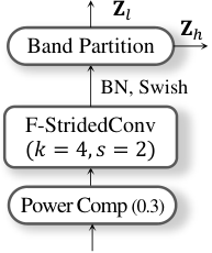
(a) Input Encoder

(b) Band Merge

(c) Filter Head

(a) T-GRU module

(b) F-self module

(c) F-cross-self module
2.2 Asymmetric encoder–decoder
The TF-Encoder applies blocks [2, 17], each an F-self module based on multi-head self-attention (MHSA) with rotary position encoding [26] and heads followed by a T-GRU module (Figure 4), to and yields . Band Merge prepares the complementary band as input-dependent queries through a residual convolution and normalization (Figure 3(b)), concatenates them with along frequency, and projects the channels from to to form . The TF-Decoder applies blocks, each an F-cross-self module followed by a T-GRU module. In the cross-self module only the complementary positions query through multi-head cross-attention (high-band MHCA) with heads; the low-band positions bypass it. A full-band MHSA with heads over all positions then relates the two bands. Both modules follow TF-Restormer [22] and use convolutional efficient feed-forward networks (ConvEFN) on a length-reduced sequence [23]: MHSA between two ConvEFNs in the F-self module, and high-band MHCA, full-band MHSA, and one ConvEFN in sequence in the F-cross-self module, with hidden widths and and two-group convolutions. The T-GRU module stacks two unidirectional GRU residual units.
2.3 Deep filtering
Let denote the noisy STFT coefficient at frame and bin , and let collect its neighboring coefficients in time and frequency. The Filter Head (Figure 3(c)) mixes the decoder channels with a pointwise convolution, restores the STFT frequency resolution with a transposed convolution along frequency, and estimates the complex filter tensor with a convolutional layer. Following the three-component estimation structure of SR-CorrNet [24], three real vectors per bin give . As in deep filtering [10, 21], the enhanced STFT is , and the SFI-iSTFT reconstructs the waveform. The compressed features determine the filter, but the samples being combined are the uncompressed observations.
| Rate (kHz) | MACs | Model | PESQ↑ | STOI↑ | SI-SDR↑ | LSD↓ | LSD |
|---|---|---|---|---|---|---|---|
| 16 | – | Noisy | 1.97 | 0.921 | 8.47 | 1.193 | – |
| 2.17G | Universal | 3.46 | 0.952 | 19.69 | 0.619 | – | |
| 16k only | 3.35 | 0.950 | 19.20 | 0.624 | – | ||
| 48k only∗ | 3.03 | 0.928 | 18.08 | 0.804 | – | ||
| 24* | – | Noisy | 1.97 | 0.921 | 8.44 | 1.297 | 1.349 |
| 2.63G | Universal | 3.44 | 0.952 | 19.62 | 0.651 | 0.560 | |
| 16k only | 3.34 | 0.949 | 19.13 | 0.660 | 0.549 | ||
| 48k only | 3.18 | 0.939 | 18.58 | 0.758 | 0.702 | ||
| 32* | – | Noisy | 1.97 | 0.921 | 8.43 | 1.288 | 1.269 |
| 3.14G | Universal | 3.47 | 0.953 | 19.47 | 0.660 | 0.595 | |
| 16k only | 3.31 | 0.949 | 19.07 | 0.691 | 0.628 | ||
| 48k only | 3.29 | 0.946 | 18.60 | 0.725 | 0.691 | ||
| 44.1* | – | Noisy | 1.97 | 0.921 | 8.42 | 1.314 | 1.290 |
| 4.03G | Universal | 3.47 | 0.952 | 18.27 | 0.721 | 0.705 | |
| 16k only | 3.23 | 0.949 | 18.96 | 0.748 | 0.722 | ||
| 48k only | 3.34 | 0.949 | 17.61 | 0.751 | 0.752 | ||
| 48 | – | Noisy | 1.97 | 0.921 | 8.41 | 1.314 | 1.285 |
| 4.35G | Universal | 3.47 | 0.951 | 18.27 | 0.729 | 0.720 | |
| 16k only∗ | 3.22 | 0.949 | 18.99 | 0.785 | 0.777 | ||
| 48k only | 3.35 | 0.949 | 17.74 | 0.735 | 0.730 |
3 Experimental setup
3.1 Datasets and evaluation metrics
We evaluate on the 824-utterance VoiceBank+DEMAND (VBD) test set at 16 and 48 kHz [28]; its fixed mixtures use SNRs of dB. The 16-kHz data are the official 28-speaker VBD training pairs at dB, divided into 10,413 training and 1,159 validation utterances. The 48-kHz training data mix clean VCTK speech [31] from 98 training and seven validation speakers, excluding both test speakers, with DNS full-band noise [3] at an integer SNR drawn uniformly from dB. VCTK utterances overlapping the VBD validation set are removed from the 48-kHz pool.
We report wideband PESQ [14], STOI [27], SI-SDR [9], and log-spectral distance (LSD) over the full input band and above 8 kHz (LSD>8k, up to the input Nyquist frequency and hence undefined at 16 kHz). Inference runs at the input rate; SI-SDR and LSD are computed at that rate against the original clean signal, whereas PESQ and STOI are computed after resampling to 16 kHz. For the multi-rate evaluation the same 48-kHz test pairs are resampled to 16, 24, 32, and 44.1 kHz. We measure multiply–accumulate operations (MACs) for one second of input using ptflops.
3.2 Training and model configuration
We train the universal model by alternating 16-kHz VBD and 48-kHz VCTK+DNS batches. We use 20 epochs of 20,000 minibatches each (400,000 in total), batch size 2, 2-s crops, and AdamP [8] (weight decay 1e-2, ). The learning rate is warmed up for 1,000 steps to 2e-3 and then cosine-decayed to 1e-6. Training draws cutoffs uniformly from kHz for 48-kHz batches and kHz for 16-kHz batches. One checkpoint per model is used for all reported input rates and inference cutoffs. We use the objective of FastEnhancer [1], , with power-compressed spectral terms. We use the TF-Refiner-B configuration in Table 3. The model applies deep filtering over a TF neighborhood (: one past and one future frame, bin), with convolutions in Band Merge and filter prediction. Each convolution adds one future frame, giving a 40-ms look-ahead and, with the 40-ms window, an 80-ms algorithmic latency. The default cutoff is kHz.
4 Results
4.1 Universal enhancement across sampling rates
Table 1 evaluates the universal model trained at 16 and 48 kHz. The two rate-specific counterparts are trained only on data at their respective rate. The universal model maintains comparable perceptual quality at the unseen rates and improves every metric over the noisy input. It obtains the best PESQ, STOI, and LSD at every rate and the best SI-SDR up to 32 kHz, whereas the 16-kHz model keeps the highest SI-SDR at 44.1 and 48 kHz, presumably because its training is confined to the power-dominant low band. The rate-specific models also transfer to unseen input rates without adaptation, although their PESQ decreases gradually. With the default cutoff of kHz, the computational cost grows by about 2.0 times from 16 to 48 kHz, whereas the number of bins triples, because the encoder analysis band remains fixed while only the shallow decoder processes the wider observed band.
Because the VBD speech is drawn from VCTK, the two training streams do not provide disjoint clean-speech corpora; they differ mainly in sampling bandwidth and corruption generation. Combining VBD pairs with VCTK+DNS mixtures may therefore contribute to the universal model’s advantage, but the 48-kHz-only model already uses the larger VCTK+DNS pool yet remains below the universal model at its native rate. We note that Table 1 does not isolate the contributions of data diversity and joint sampling-rate exposure.
| Method | Param | 16 kHz | 48 kHz | ||||
|---|---|---|---|---|---|---|---|
| MACs | PESQ | SI-SDR | MACs | PESQ | SI-SDR | ||
| Noisy | – | – | 1.97 | 8.47 | – | 1.97 | 8.41 |
| GTCRN [15] | 0.02M | 0.04G | 2.87 | 18.83 | – | – | – |
| UL-UNAS [16] | 0.17M | 0.03G | 3.09 | 18.48 | – | – | – |
| FastEnhancer-B [1] | 0.09M | 0.26G | 3.13 | 19.0 | – | – | – |
| FastEnhancer-S [1] | 0.20M | 0.66G | 3.19 | 19.2 | – | – | – |
| FastEnhancer-M [1] | 0.49M | 2.90G | 3.24 | 19.4 | – | – | – |
| TF-Refiner-B (16k) | 0.47M | 2.17G | 3.35 | 19.20 | 4.35G | 3.22* | 18.99* |
| PercepNet [29] | 8.00M | – | – | – | 0.80G | 2.73 | – |
| DeepFilterNet [20] | 1.78M | – | – | – | 0.35G | 2.81 | 16.63 |
| DMF-Net [33] | 7.84M | – | – | – | – | 2.97 | – |
| DeepFilterNet2 [19] | 2.31M | – | – | – | 0.36G | 3.08 | – |
| TF-Refiner-B (48k) | 0.47M | 2.17G | 3.03* | 18.08* | 4.35G | 3.35 | 17.74 |
| TF-Refiner-B | 0.47M | 2.17G | 3.46 | 19.69 | 4.35G | 3.47 | 18.27 |
| TF-Refiner-T† | 0.09M | 0.54G | 3.20 | 19.07 | 1.27G | 3.10 | 17.07 |
| TF-Refiner-S† | 0.19M | 0.97G | 3.37 | 19.42 | 2.03G | 3.36 | 18.36 |
| TF-Refiner-B† | 0.45M | 2.05G | 3.30 | 19.42 | 3.85G | 3.36 | 18.41 |
4.2 Configurable computation
Figure 5 compares the universal model with fixed-cutoff controls while changing at inference for every model. The controls use the same 16/48-kHz training with fixed at 1, 2, 3, 5, 8, 12, or 16 kHz. The total MACs increase with because more positions enter the deep encoder. Fixed-cutoff models degrade as the inference cutoff moves far from their training cutoff. Random-cutoff training keeps the universal model close to the best fixed-cutoff model in PESQ and LSD over 2–8 kHz (2–7 kHz for 16-kHz input), while the fixed-cutoff models retain an advantage at the extremes.
Lowering from the default 5 to 3 kHz reduces the cost by 29% at 16 kHz and 16% at 48 kHz with a small PESQ decrease. At lower cutoffs, the universal model also degrades more gradually than the model trained at a fixed 5-kHz cutoff. At 48 kHz, the model trained and evaluated at kHz costs about twice as much as the universal model at the default cutoff without a higher PESQ.
| Model | Encoder | Decoder | ||||||
|---|---|---|---|---|---|---|---|---|
| TF-Refiner-T | 4 | 24 | 42 | 4 | 2 | 12 | 24 | 2 |
| TF-Refiner-S | 4 | 32 | 88 | 4 | 2 | 16 | 48 | 4 |
| TF-Refiner-B | 4 | 48 | 144 | 4 | 2 | 24 | 72 | 4 |
4.3 Comparison with published systems
Table 2 compares published systems at their native rates with TF-Refiner variants, each using one parameter set at both rates. For single-rate comparisons, we include TF-Refiner-B (16k) and TF-Refiner-B (48k), the rate-specific models of Table 1. At the default kHz, TF-Refiner-B (16k) achieves a PESQ of 3.35 versus 3.24 for FastEnhancer-M at 16 kHz, while its SI-SDR is 0.2 dB lower. TF-Refiner-B (48k) achieves a PESQ of 3.35 versus 3.08 for DeepFilterNet2 [19] at 48 kHz. The universal TF-Refiner-B further increases PESQ to 3.46 and 3.47 at 16 and 48 kHz, respectively.
The no-look-ahead variants (†) use frequency-only convolutions with kernel size 3 in Band Merge and filter prediction, with same-frame frequency taps, giving a 40-ms algorithmic latency. TF-Refiner-B† also outperforms the published systems in PESQ at both rates. For scaling, we evaluate the tiny and small no-look-ahead variants using the configurations in Table 3. S† maintains comparable quality to B† at substantially lower cost, while T† trades some quality for further savings.
4.4 Ablation study
| Model | PESQ↑ | STOI↑ | SI-SDR↑ | LSD↓ | LSD |
|---|---|---|---|---|---|
| TF-Refiner-B (48k) | 3.35 | 0.949 | 17.74 | 0.735 | 0.730 |
| w/o high-band MHCA | 3.31 | 0.950 | 17.40 | 0.782 | 0.794 |
| w/o Band Merge conv. | 3.34 | 0.950 | 17.39 | 0.767 | 0.773 |
| w/ direct mapping | 3.11 | 0.944 | 15.95 | 0.801 | 0.812 |
Table 4 ablates the modules that connect the analysis band to the full-band output. Removing high-band MHCA, through which the high-band queries attend to the encoder output, or the Band Merge convolution that forms those queries changes PESQ and STOI, which assess only the band below 8 kHz, by at most 0.04 but costs about 0.3 dB of SI-SDR and raises LSD>8k from 0.730 to 0.794 and 0.773, respectively. Both modules thus mainly serve the observed high band. Replacing local filtering with direct complex mapping degrades every metric, lowering SI-SDR by 1.8 dB and raising LSD by 0.07, consistent with the filter preserving the fine structure of the observed STFT.
5 Conclusion
We presented TF-Refiner, a sampling-frequency-independent full-band speech enhancement model whose deep analysis is confined to a configurable band while a shallow decoder refines the observed remainder and filters the original noisy STFT. One universal model enhances 16- to 48-kHz inputs, including unseen rates, and the analysis cutoff selects a cost–quality operating point at inference without changing the architecture or retraining. Future work includes evaluation on unseen corpora and streaming latency measurement.
References
- [1] (2026) FastEnhancer: speed-optimized streaming neural speech enhancement. In Proc. IEEE ICASSP, pp. 16847–16851. External Links: Document Cited by: §1, §3.2, Table 2, Table 2, Table 2.
- [2] (2022) DPT-FSNet: dual-path transformer based full-band and sub-band fusion network for speech enhancement. In Proc. IEEE ICASSP, pp. 6857–6861. External Links: Document Cited by: §1, §2.2.
- [3] (2022) ICASSP 2022 deep noise suppression challenge. In Proc. IEEE ICASSP, pp. 9271–9275. External Links: Document Cited by: §1, §3.1.
- [4] (2026) One model, many latencies: universal speech enhancement for diverse real-time applications. Note: arXiv:2606.25621 External Links: 2606.25621 Cited by: §1.
- [5] (2023) Siamese masked autoencoders. In Proc. NeurIPS, pp. 40676–40693. External Links: Document Cited by: §1.
- [6] (2021) FullSubNet: a full-band and sub-band fusion model for real-time single-channel speech enhancement. In Proc. IEEE ICASSP, pp. 6633–6637. External Links: Document Cited by: §1.
- [7] (2022) Masked autoencoders are scalable vision learners. In Proc. IEEE/CVF CVPR, pp. 15979–15988. External Links: Document Cited by: §1.
- [8] (2021) AdamP: slowing down the slowdown for momentum optimizers on scale-invariant weights. In Proc. ICLR, External Links: Link Cited by: §3.2.
- [9] (2019) SDR – half-baked or well done?. In Proc. IEEE ICASSP, pp. 626–630. External Links: Document Cited by: §3.1.
- [10] (2020) Deep filtering: signal extraction and reconstruction using complex time-frequency filters. IEEE SPL 27, pp. 61–65. External Links: Document Cited by: §1, §2.3.
- [11] (2014) Detection of high-frequency energy level changes in speech and singing. J. Acoust. Soc. Am. 135 (1), pp. 400–406. External Links: Document Cited by: §1.
- [12] (2016) A review of the perceptual effects of hearing loss for frequencies above 3 kHz. Int. J. Audiol. 55 (12), pp. 707–714. External Links: Document Cited by: §1.
- [13] (2022) Sampling frequency independent dialogue separation. In Proc. EUSIPCO, pp. 160–164. External Links: Document Cited by: §1, §2.1.
- [14] (2001) Perceptual evaluation of speech quality (PESQ)—a new method for speech quality assessment of telephone networks and codecs. In Proc. IEEE ICASSP, pp. 749–752. External Links: Document Cited by: §3.1.
- [15] (2024) GTCRN: a speech enhancement model requiring ultralow computational resources. In Proc. IEEE ICASSP, pp. 971–975. External Links: Document Cited by: §1, Table 2.
- [16] (2026) UL-UNAS: ultra-lightweight U-Nets for real-time speech enhancement via network architecture search. IEEE TASLP 34, pp. 1085–1096. External Links: Document Cited by: §1, Table 2.
- [17] (2024) TF-Locoformer: transformer with local modeling by convolution for speech separation and enhancement. In Proc. IWAENC, pp. 205–209. External Links: Document Cited by: §1, §2.2.
- [18] (2022) Sampling-frequency-independent convolutional layer and its application to audio source separation. IEEE/ACM TASLP 30, pp. 2928–2943. External Links: Document Cited by: §1.
- [19] (2022) DeepFilterNet2: towards real-time speech enhancement on embedded devices for full-band audio. In Proc. IWAENC, pp. 1–5. External Links: Document Cited by: §1, §1, §4.3, Table 2, Table 2.
- [20] (2022) DeepFilterNet: a low complexity speech enhancement framework for full-band audio based on deep filtering. In Proc. IEEE ICASSP, pp. 7407–7411. External Links: Document Cited by: §1, Table 2, Table 2.
- [21] (2026) Deep filter estimation from inter-frame correlations for monaural speech dereverberation. Note: arXiv:2603.14986 External Links: 2603.14986 Cited by: §1, §2.3.
- [22] (2026) Query-based asymmetric modeling with decoupled input-output rates for speech restoration. In Proc. ICML, External Links: Link Cited by: §1, §1, §2.1, §2.2.
- [23] (2024) Separate and reconstruct: asymmetric encoder-decoder for speech separation. In Proc. NeurIPS, External Links: Link Cited by: §2.2.
- [24] (2026) Asymmetric encoder-decoder based on time-frequency correlation for speech separation. Note: arXiv:2603.29097 External Links: 2603.29097 Cited by: §2.3.
- [25] (2001) Effect of stimulus bandwidth on the perception of /s/ in normal- and hearing-impaired children and adults. J. Acoust. Soc. Am. 110 (4), pp. 2183–2190. External Links: Document Cited by: §1.
- [26] (2024) RoFormer: enhanced transformer with rotary position embedding. Neurocomputing 568. Note: Art. no. 127063 External Links: Document Cited by: §2.2.
- [27] (2011) An algorithm for intelligibility prediction of time–frequency weighted noisy speech. IEEE TASLP 19 (7), pp. 2125–2136. External Links: Document Cited by: §3.1.
- [28] (2017) Noisy speech database for training speech enhancement algorithms and TTS models. Note: University of Edinburgh, doi:10.7488/ds/2117 External Links: Document, Link Cited by: §3.1.
- [29] (2020) A perceptually-motivated approach for low-complexity, real-time enhancement of fullband speech. In Proc. Interspeech, pp. 2482–2486. External Links: Document Cited by: §1, §1, Table 2.
- [30] (2018) A hybrid DSP/deep learning approach to real-time full-band speech enhancement. In Proc. IEEE MMSP, pp. 1–5. External Links: Document Cited by: §1, §1.
- [31] (2017) CSTR VCTK corpus: english multi-speaker corpus for CSTR voice cloning toolkit. Note: University of Edinburgh, https://hdl.handle.net/10283/2950 External Links: Link Cited by: §3.1.
- [32] (2023) TF-GridNet: integrating full- and sub-band modeling for speech separation. IEEE/ACM TASLP 31, pp. 3221–3236. External Links: Document Cited by: §1.
- [33] (2022) DMF-Net: a decoupling-style multi-band fusion model for full-band speech enhancement. In Proc. APSIPA ASC, pp. 1382–1387. External Links: Document Cited by: §1, §1, Table 2.
- [34] (2024) Improving design of input condition invariant speech enhancement. In Proc. IEEE ICASSP, pp. 10696–10700. External Links: Document Cited by: §1.
- [35] (2023) Toward universal speech enhancement for diverse input conditions. In Proc. IEEE ASRU, pp. 1–6. External Links: Document Cited by: §1.