Adaptive State Estimation Under Topological Uncertainty in Unobservable Primary Distribution Systems Using Strategically Placed Sensors
Thanks: This work was supported by the U.S. Department of Energy (DOE) grant DE-OE0000983.
The views expressed herein do not necessarily represent the views of the U.S. Department of Energy or the United States Government.
Abstract
The rapid integration of distributed energy resources is fundamentally altering power flow patterns in primary distribution networks and intensifying operational uncertainty. These problems are further compounded by lack of real-time situational awareness and frequent topology changes. To address these problems, this paper proposes an integrated deep learning framework for simultaneous topology identification (TI) and distribution system state estimation (DSSE) in real-time unobservable primary distribution networks instrumented by a minimal set of synchronized measurement devices (SMDs). A correlation-driven SMD placement algorithm is introduced first that jointly satisfies TI accuracy and DSSE performance requirements by exploiting temporal and spatial correlations in nodal voltage measurements. A dual deep neural network (DNN)-based DSSE model is developed next to estimate three-phase voltage magnitudes and angles across diverse operating conditions. To extend the framework beyond the base topology, fine-tuning-based transfer learning is employed to adapt the DSSE model to reconfigured topologies using limited retraining data. The framework is validated under both Gaussian and non-Gaussian measurement noise and benchmarked against a conventional estimation approach and a single DNN model.
Index Terms:
Deep learning, State estimation, Synchronized measurement device, Topology identification, Transfer learningI Introduction
The rapid integration of distributed energy resources (DERs) is fundamentally reshaping power flow patterns in distribution networks. High DER penetration introduces voltage fluctuations, reverse power flows, and localized violations that can propagate deep into the feeder and remain entirely undetected without adequate real-time monitoring. Achieving real-time situational awareness is therefore a prerequisite for reliable and secure distribution grid operation and control [1, 2].
However, the primary circuit of the distribution system is critically under-instrumented in the context of real-time situational awareness. Smart meters, which offer spatially dense coverage and report at 15-minute to hourly intervals, have latencies of several hours; they are also placed on the secondary circuits. SCADA systems provide faster updates but their observability is effectively confined to the feeder head [3]. Synchronized measurement devices (SMDs), such as phasor measurement units (PMUs) and micro-PMUs (PMUs), provide millisecond-resolution time-synchronized measurements for distribution system state estimation (DSSE) [4]. However, the high deployment cost of SMDs keeps practical installations extremely sparse. Field measurements also confirm that SMD noise is better characterized by non-Gaussian models than the Gaussian assumption adopted in conventional estimators [5].
In this regard, deep neural network (DNN)-based state estimators have been developed to address both unobservability [6] as well as non-Gaussian noise [7]. Particularly, [7] went a step further to not only present a unified DNN framework for simultaneous three-phase unbalanced DSSE and topology identification (TI) using sparse SMD measurements, but also created an SMD placement scheme exclusively for DNNs, demonstrating that DNN-based estimators achieve accurate joint estimation with far fewer sensors than conventional estimators. However, the sensor placement in [7] was derived from spatial correlation analysis at a single hour, implying that it could not account for temporal variability of voltages occurring across different hours of the day. Moreover, the voltage magnitude and angle in [7] were estimated by a single unified DNN, which we demonstrate produces inferior performance compared to dedicated models for each quantity.
This paper proposes a comprehensive framework for deep learning-based time-synchronized TI and three-phase unbalanced DSSE to ensure reliable operation across all hours of the day in real-time unobservable primary distribution networks. The specific contributions are:
- 1.
A correlation-driven SMD placement algorithm that jointly optimizes sensor locations for both TI and DSSE by incorporating temporal variability and spatial correlation of all nodal voltage phasors.
- 2.
Dual DNN-based DSSE models that independently estimate three-phase voltage magnitude and angles, demonstrating superior accuracy over a single unified model across different hours of the day and under both Gaussian and non-Gaussian noise.
- 3.
A fine tuning (FT)-based transfer learning (TL) strategy that adapts the base-topology DSSE model to reconfigured network topologies using limited retraining data, triggered automatically by the DNN-based TI model upon topology change detection.
The overall framework is illustrated in Fig. 1. In the offline phase, historical smart meter data from advanced metering infrastructure (AMI) is used to learn distributions that characterize the aggregated loads at the primary network-level. In parallel, a correlation-driven SMD placement algorithm identifies the required sensor locations for joint TI and DSSE. In the online phase, real-time PMU/PMU measurements are fed into the DNN-based TI model, which continuously monitors switch statuses and detects topology changes. Simultaneously, the DNN-based DSSE models produce three-phase voltage phasor estimates for all the nodes. If the DNN-TI detects a topology change, then TL is used to update the DNN-DSSE to adapt it to the new network configuration.

II Temporally-Aware Correlation-Driven SMD Placement
Time-synchronized joint TI and DSSE in an incompletely observed distribution network requires SMD locations that simultaneously capture discriminative switching information and are spatially representative of the full network voltage profile. These objectives place competing demands on sensor placement considering TI favors locations sensitive to current redistribution under switching events, while DSSE favors locations that maximize spatial voltage coverage. A placement optimized for either objective alone will underperform on the other task. Furthermore, distribution networks with significant DER penetration operate under substantially different loading and generation conditions across different hours of the day. A sensor placement strategy derived from a single hour (as done in [7]) may fail to provide adequate coverage during other hours. The proposed algorithm addresses these concerns by integrating temporal correlation analysis with spatial correlation-driven SMD placement to satisfy TI accuracy and DSSE performance thresholds simultaneously for all primary circuit voltages across multiple hours.
II-A Temporal Correlation Analysis
The goal of this stage is to identify a set of representative time slots whose collective voltage statistics span the full diversity of diurnal operating conditions, ensuring that the subsequent sensor placement is valid for all hours of the day. The procedure is illustrated in Fig. 2, and elaborated below.
Historical smart meter data provides hourly net active and reactive power injections at each primary load node. Using these injections, large numbers of power flows are solved to produce time-series voltage phasor profiles across all network nodes (denoted by ). A kernel density estimator (KDE) is then fitted to the voltage magnitude at each node for each hour , capturing the non-Gaussian, multimodal character of residential load distributions without imposing a parametric form [8]. Next, the Jensen-Shannon divergence (JSD) is computed between the voltage magnitude distributions of every pair of hours at each node , yielding a pairwise dissimilarity matrix . Finally, the are averaged across all the nodes to obtain a system-wide dissimilarity matrix, :
| (1) |
Next, hierarchical clustering with average linkage is applied to . The resulting dendrogram is cut where the inter-cluster distance increases most sharply The threshold of 0.5 is selected at the largest dendrogram merge gap, yielding ; a lower threshold of 0.4 would produce a third cluster of only 2 hours, which is insufficient to capture the diversity of that regime.

II-B SMD Placement for TI and DSSE
The second stage performs SMD placement using the representative time slots as one of its inputs. The other inputs are the sensor budget, a TI accuracy threshold , a DSSE spatial correlation threshold , and the number of nodes , while the output is the required SMD location set . The complete procedure is summarized in Algorithm 1.
II-B1 Part A: Placement for TI
Part A identifies the minimum SMD set whose current phasor measurements enable the DNN-TI model to achieve accuracy across all time slots. This is formulated as a sequential forward selection (SFS) problem, where locations are added greedily to maximize classification accuracy. Current phasors are used as the discriminative feature because topology changes alter the network admittance matrix and redistribute power flows, producing dominant changes in branch current magnitudes and angles at locations electrically close to the switching event.
II-B2 Part B: Placement for DSSE
Part B augments with additional SMDs to ensure that every unmonitored node has a Spearman correlation coefficient (SCC) of at least with at least one node already in . The SCC, computed as shown in (2), is evaluated per feeder/voltage-regulated zone:
| (2) |
This iterative coupling ensures that both objectives are jointly satisfied across all slots once the TI and DSSE thresholds are met.
III Dual-Model Deep Inference for Topology and Voltage Phasor Estimation
In the proposed framework, TI and DSSE are handled by separate models rather than a single multi-task network. TI requires classification over a discrete topology space while DSSE requires regression over a continuous high-dimensional voltage phasor space. Jointly optimizing both under a shared objective constrains the expressivity available to each task; separate models allow each network to fully specialize its learned representations. The general DNN architecture shared across all models is illustrated in Fig. 3, where denotes the SMD measurement input vector and denotes the output, representing either topology class probabilities (for the TI model) or estimated voltage phasors (for the DSSE model).

III-A DNN-Based Topology Identification (TI)
The TI model takes as input the three-phase current phasor measurements (magnitude and angle) from all SMD locations in , and performs multi-class classification over all feasible network topologies, where each topology corresponds to a unique combination of switch statuses and is assigned a unique integer label. This formulation naturally handles multiple simultaneous switching operations and scales to large numbers of switches [7]. The model is a fully connected feedforward DNN with hidden layers regularized by batch normalization and dropout. Batch normalization stabilizes training by reducing internal covariate shift, while dropout mitigates overfitting by stochastically deactivating neurons during training. Hyperparameters are tuned using the Keras Tuner framework and reported in Section V.
III-B Dual DNN-Based State Estimation
The DSSE models take as input both voltage and current phasor measurements from the SMD locations in . Voltage measurements provide direct local observability at instrumented nodes and serve as anchor points from which the network-wide voltage profile is inferred, while current measurements carry the power flow information necessary to reconstruct unmonitored node voltages. Two regression models are trained independently in parallel, one for three-phase voltage magnitudes and the other for three-phase voltage angles, across all nodes. This dual-model design is motivated by the observation that voltage magnitudes and angles exhibit fundamentally different spatial correlation structures and dynamic ranges across the network. A single unified model must learn both mappings simultaneously under a shared loss, constraining the internal representations available to each task. Separate models allow full specialization and, as demonstrated in Section V, consistently produce lower estimation error than the unified approach, particularly when evaluated across multiple operating time slots where the statistical characteristics of magnitude and angle distributions diverge.
Each model is a fully connected feedforward DNN with hidden layers regularized by batch normalization and dropout. The number of hidden layers, neurons per layer, and dropout rate are determined independently for each model and each representative time slot using the Keras Tuner framework. The specific architectures for each slot are reported in Section V.
IV Topology-Triggered Model Adaptation Through Fine-Tuning (FT)
The dual DNN-DSSE models developed in Section III are trained on data generated from the base topology. When the network undergoes a switching operation, the marginal distribution of SMD measurements shifts because loads are now served through different paths and branch currents are redistributed accordingly. A model trained on the preceding topology will receive test inputs from a shifted distribution, degrading estimation accuracy in proportion to the structural difference between topologies. Full retraining from scratch for every new topology is theoretically sound but practically infeasible, requiring large amounts of new training data and significant computational time.
TL addresses this issue by reusing knowledge encoded in a previously trained model to accelerate learning in a new but related domain [9]. In the context of DNN-based DSSE, the source domain corresponds to the topology under which the model was most recently trained, and the target domain corresponds to the new topology after a switching event. The feature space does not change across domains since the same SMD measurements are used regardless of topology; however, the marginal distribution of those measurements does change, making adaptation necessary. Among available TL strategies, parameter-based transfer via FT is adopted. FT initializes the target-domain model with the weights of the most recently trained model and continues training on a limited amount of target-domain data, rather than from random initialization. The rationale for using FT is that distribution networks sharing the same physical infrastructure across topologies exhibit strongly overlapping voltage and current statistics. Hence, lower DNN layers learn general representations of the network’s electrical behavior, such as feeder impedance profiles and load correlation structures, that remain approximately valid after switching. Only the higher layers encoding topology-specific mappings require updating, making fine-tuning from existing weights more data-efficient than retraining from scratch.
The proposed TL framework adopts a strictly sequential adaptation strategy: whenever a topology change is detected by the DNN-TI model, the active DSSE model is fine-tuned directly from its current weights. This imposes minimal memory requirements while remaining adaptive to the evolving network configuration. Formally, let denote the DSSE model weights after the -th topology transition, trained on topology . When the network transitions to , a small dataset is used for the new topology, where (the original training set size), with chosen as the minimum number of scenarios at which post-adaptation DSSE accuracy stabilizes. The adapted model is obtained by minimizing the empirical mean-squared error (MSE) loss initialized from the current weights:
| (3) |
where is the DNN mapping. The updated model replaces the active model and is used for all subsequent inference until the next topology change is detected.
The complete sequential adaptation procedure is summarized in Algorithm 2. During real-time operation, the DNN-TI model continuously monitors incoming SMD measurements and classifies the current topology. Upon detecting a change, FT is triggered using pre-generated and stored scenarios for the detected topology, and the DSSE models resume inference post-update. The results obtained using the proposed topology-triggered model adaptation are provided in Section V for four consecutive topology transitions.
V Simulation Results
V-A Test System and Data Generation
Simulations are conducted on a 240-node US Midwest primary distribution test system that is described in [10]. The system has three feeders, and 9 sectionalizing switches yielding 84 feasible topologies. Of the 240 nodes of this system, 193 nodes have loads. One year of hourly smart meter data is publicly available for these loads. To generate training datasets of sufficient sizes for DNN training, a KDE is fitted independently to the active and reactive power injection at each load node per hour obtained from the smart meter data. Monte Carlo sampling is then done to draw new load scenarios from the learned distributions. Power flow is solved in OpenDSS [11] for each sampled scenario to obtain the corresponding voltage and current phasors. For the base-topology DNN-DSSE, 1,500 scenarios per hour are generated (36,000 total), and for DNN-TI, 100 scenarios per hour per topology are used. For FT, 150 scenarios per hour (3,600 total) are generated for each target topology. Three noise models are applied to SMD measurements to evaluate robustness, namely, Gaussian , Gaussian mixture model (GMM) as a two-component mixture , and Laplacian . The last two represent non-Gaussian characteristics consistent with field SMD measurements [5]. All simulations are conducted on a server equipped with dual Intel Xeon Platinum 8368 processors (76 cores, 152 logical processors at 2.40 GHz) and 384 GB of DDR4-3200 RAM.
V-B Proposed DNN-Based TI and DSSE
The JSD-based hierarchical clustering partitions the 24 hours of the day into representative time slots at a distance threshold of 0.5, as shown in the dendrogram of Fig. 4. Slot 1 captures daytime and evening hours (7–22) with higher voltage variability, while Slot 2 corresponds to overnight hours (22–7) with lower voltage variability. Applying Algorithm 1 with and , yields 7 SMD locations after Slot 1 and one additional location after incorporating Slot 2, resulting in a total of 8 locations for placing SMDs.
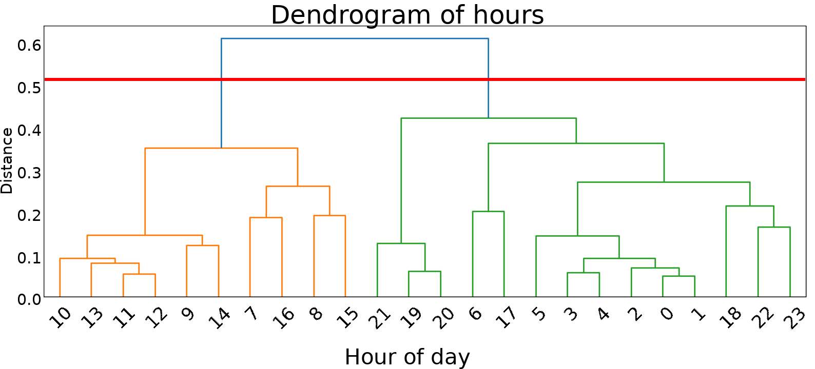
Fig. 5 compares the three SMD placement strategies, namely, TI-only, DSSE-only, and the proposed integrated placement, under all three noise conditions and for both time slots. The DSSE-only placement consistently degrades TI accuracy to the 88–91% range, falling below the 99% operational threshold regardless of noise type or time slot. The TI-only placement maintains high TI accuracy but fails to meet DSSE spatial coverage requirements. The integrated placement satisfies both objectives simultaneously across all noise types and time slots, achieving TI accuracy above 99.9%, magnitude MAPE within 0.04%, and angle MAE within 0.03∘. The SMD locations for the integrated placement and corresponding performance metrics are reported in the last row of Table I.

| Model | Slot | Phase MAE (∘) | Mag. MAPE (%) |
| Single Unified DNN | Slot 1 | 0.019 | 0.031 |
| Slot 2 | 0.044 | 0.062 | |
| Dual DNN (proposed) | Slot 1 | 0.010 | 0.015 |
| Slot 2 | 0.023 | 0.026 | |
| SMD locations: 1–1001, 1008–1009, 2011–2012, 2019–2021, 3003–3005, 3068–3075, 3081–2016 (inter-feeder B–C link), 3137–3138 | |||
Table I benchmarks the proposed dual-model design against a single unified DNN estimating both magnitude and angle simultaneously under GMM noise for both time slots. The proposed dual model reduces Mag. MAPE by 52% and Ang. MAE by 47% in Slot 1, and by 58% and 48%, respectively, in Slot 2, confirming that specialized models consistently outperform a single unified estimator across both operating regimes. The larger degradation of the single unified model in Slot 2 further confirms that when trained for one representative hour, the single model struggles to generalize across other operating envelopes.
The DNN architectures for the base topology under GMM noise are summarized in Table II. The TI model uses a deeper 6-layer network with 800 neurons per layer to resolve the 84-class topology space, while the DSSE magnitude and angle models use shallower architectures independently tuned by Keras Tuner. The fine-tuned model inherits the base architecture with a reduced learning rate of and only 50 epochs, enabling rapid adaptation upon topology change.
| Parameter | DNN-TI | DNN-DSSE | FT | |
| Mag | Ang | |||
| Inputs | 48 (I) | 92 (V&I of SMDs) | ||
| Outputs | 84 (topo) | 462 (states) | ||
| Hidden layers | 6 | 2 | ||
| Neurons/layer | 800 | 640 | 256 | |
| Dropout | 0.3 | 0.5 | ||
| Hidden activ. | ReLU | |||
| Output activ. | Softmax | Linear | ||
| Optimizer | Adam | |||
| Loss | Categorical cross-entropy | MSE | ||
| Epochs | 100 | 200 | 50 | |
| Batch size | 105 | 32 | 32 | |
| Learning rate | ||||
| Samples/hour | 8400 | 1500 | 150 | |
Table III compares the proposed DNN-based approach to linear state estimation (LSE) under Gaussian and non-Gaussian (GMM) noises for both time slots. LSE requires full observability and is implemented with 113 SMD locations (determined using the approach developed in [12]), while the proposed DNN operates with only 8 SMDs, about a 93% reduction in instrumentation needs. The DNN achieves slightly worse results than LSE (particularly in the magnitudes), while it has similar results under Gaussian and GMM noises, demonstrating its robustness to different noise models.
| Model | Slot 1 | Slot 2 | #SMDs | ||
| MAE | MAPE | MAE | MAPE | ||
| LSE (Gaussian) | 0.001∘ | 0.015% | 0.001∘ | 0.014% | 113 |
| DNN (Gaussian) | 0.017∘ | 0.018% | 0.024∘ | 0.026% | 8 |
| DNN (GMM) | 0.010∘ | 0.015% | 0.028∘ | 0.064% | 8 |
V-C TL for Topology Adaptation
Fig. 6 shows MAPE and MAE across the topology transition sequence under GMM noise for Slot 1. Table IV reports the exact metrics and training times for the sequence: , for three conditions, namely, no adaptation, FT, and complete retraining. differs from in five switch positions and in two switch positions, exercising both large and moderate topological shifts. Without adaptation, MAPE degrades to 0.072–0.090% and angle MAE reaches up to 0.098∘. FT helps maintain accuracies of 0.025–0.027% MAPE and 0.018–0.020∘ MAE, which approaches complete-retraining accuracy at a fraction of the computational cost/time. The return to demonstrates that sequential FT from an intermediate model state is sufficient for accurate recovery even when revisiting a previously encountered topology, without storing any model checkpoints. Exact metrics for all transitions are reported in Table IV.

| Metric | Tbase | TbaseT36 | T36T2 | T2Tbase |
| MAPE (%) | 0.015 | 0.026 | 0.027 | 0.025 |
| MAE (∘) | 0.010 | 0.020 | 0.018 | 0.018 |
| Mag. train time (s) | 1480 | 31 | 28 | 27 |
| Ang. train time (s) | 947 | 44 | 43 | 43 |
VI Conclusion
This paper proposed an integrated deep learning framework for simultaneous TI and three-phase unbalanced DSSE in real-time unobservable primary networks instrumented by a minimal set of SMDs. The framework is validated using a 240-node real-world test system under full operational variability. A correlation-driven placement algorithm was introduced first that jointly optimized sensor locations for both TI and DSSE by exploiting temporal variability across different hours via JSD-based hierarchical clustering and spatial correlation of nodal voltage phasors via SCC-based rank analysis. For the identified test system, the algorithm identified two representative time slots and converged to 8 SMD locations satisfying both a TI accuracy threshold and a SCC threshold simultaneously across all noise conditions, compared to 113 SMD locations required by conventional LSE.
Dedicated dual DNN-DSSE models for voltage magnitude and angle were developed next and it was shown that they outperformed a single unified estimator by up to in magnitude MAPE and in angle MAE under GMM noise, with consistent gains across both time slots. The framework demonstrated robustness under Gaussian, GMM, and Laplacian noises, maintaining TI accuracy above and DSSE errors within operational bounds in all cases. Finally, FT-based TL enabled rapid topology adaptation upon switching events, resulting in an improvement of - in MAPE and - in MAE over the no adaptation case across three consecutive topology transitions. The adaptation took place in under one minute without storing any model checkpoints, compared to - minutes for complete retraining.
References
- [1] International Energy Agency, “Solar PV Power Capacity in the Net Zero Scenario, 2015–2030,” IEA, 2023. [Online]. Available: https://www.iea.org/energy-system/renewables/solar-pv
- [2] D. Dalal, M. Sondharangalla, R. Ayyanar, and A. Pal, “Improving Photovoltaic Hosting Capacity of Distribution Networks with Coordinated Inverter Control: A Case Study of the EPRI J1 Feeder”. IET Renewable Power Generation, vol. 19, no. 1, p.e13181, Jan. 2025.
- [3] B. Azimian, R. S. Biswas, and A. Pal, “Application of AI and Machine Learning Algorithms in Power System State Estimation”. Smart Cyber‐Physical Power Systems: Solutions from Emerging Technologies, Vol. 2, pp. 93-130, 2025.
- [4] R. Arghandeh et al., “Synchronized Measurements and their Applications in Distribution Systems: An Update,” NASPI Distribution Task Team, Tech. Rep. NASPI-2020-TR-016, Jun. 2020.
- [5] B. Azimian, R. S. Biswas, A. Pal, and L. Tong, “Time Synchronized State Estimation for Incompletely Observed Distribution Systems Using Deep Learning Considering Realistic Measurement Noise,” Proc. IEEE Power & Energy Society General Meeting (PESGM), Washington, DC, USA, 2021, pp. 1-5.
- [6] K. Mestav, J. Luengo-Rozas, and L. Tong, “Bayesian State Estimation for Unobservable Distribution Systems via Deep Learning,” IEEE Trans. Power Syst., vol. 34, no. 6, pp. 4910–4920, Nov. 2019.
- [7] B. Azimian, R. Sen Biswas, A. Pal, L. Tong, and G. Dasarathy, “State and Topology Estimation for Unobservable Distribution Systems Using Deep Neural Networks,” IEEE Trans. Instrum. Meas., vol. 71, p. 9003514, 2022.
- [8] E. Parzen, “On Estimation of a Probability Density Function and Mode,” Ann. Math. Stat., vol. 33, no. 3, pp. 1065–1076, 1962.
- [9] S. J. Pan and Q. Yang, “A Survey on Transfer Learning,” IEEE Trans. Knowl. Data Eng., vol. 22, no. 10, pp. 1345–1359, Oct. 2010.
- [10] F. Bu, Y. Yuan, Z. Wang, K. Dehghanpour, and A. Kimber, “A Time-Series Distribution Test System Based on Real Utility Data,” Proc. North American Power Symp. (NAPS), Wichita, KS, 2019, pp. 1–6.
- [11] R. C. Dugan and T. E. McDermott, “An Open Source Platform for Collaborating on Smart Grid Research,” Proc. IEEE PES General Meeting, Detroit, MI, 2011, pp. 1–7.
- [12] R. S. Biswas, B. Azimian, and A. Pal, “A Micro-PMU Placement Scheme for Distribution Systems Considering Practical Constraints,” Proc. IEEE Power & Energy Society General Meeting (PESGM), Montreal, QC, Canada, 2020, pp. 1-5