Quantum computational advantage in random-circuit sampling on IBM superconducting quantum computers
Abstract
We report forward random-circuit sampling (RCS) on the 120-qubit Nighthawk r2 superconducting processor (ibm_phoenix) with square-lattice connectivity, using 61 qubits, native CZ gates, and the standard cloud execution stack with no benchmark-specific calibration. Two independent fidelity estimators—mirror benchmarking and three- and four-patch cross-entropy benchmarking (XEB)—agree with each other at every measured depth, the mirror from 4 to 40 cycles and the patched estimators from 20 to 40 cycles, across more than two orders of magnitude of fidelity decay, and exceed the first-generation Nighthawk r1 device by more than an order of magnitude at fixed depth. The 36-cycle circuits sit at the depth where tensor-network contraction cost saturates at system size: a contraction-cost estimator validated against the published Sycamore and Zuchongzhi networks places the single-amplitude cost at complex operations. At under favorable memory assumptions this implies machine operations within the bounded-fidelity rejection-sampling model — more than a century of runtime on the Frontier supercomputer — to collect a -sample ensemble, which takes only 19 s on Nighthawk r2. To our knowledge, this is the first demonstration of quantum advantage for a vanilla random-circuit sampling on a commercially and broadly accessible quantum processor that most non-expert quantum computer users can easily replicate.
I Introduction
The computational power of a quantum processor derives from the exponential growth of Hilbert-space dimension with qubit number; on near-term devices it is bounded instead by how much of that space noise leaves coherently accessible. Random-circuit sampling (RCS), scored by linear cross-entropy benchmarking (XEB), has become the standard probe of this boundary: quantum correlations spread as fast as the geometry allows, and hardness rests on anticoncentration and average-case conjectures for the output probabilities; what the experiment actually reports is one number, a fidelity proxy [37, 1, 9, 35, 11, 13, 33, 22]. Since the 53-qubit Sycamore experiment [4], the quantum side of this competition has advanced through Zuchongzhi 2.0 and 2.1 [44, 46], Sycamore at 67 qubits [32], and Zuchongzhi 3.0 at 83 active qubits and 32 cycles [16], while the classical side has cut the cost of Sycamore-class verification and sampling by orders of magnitude [8, 12, 41, 24, 27, 20, 26, 36, 28, 45]. The competition has also sharpened what such claims mean. XEB certifies no total-variation closeness: it can be spoofed in exploitable regimes, and it tracks fidelity only in a limited window of depth and noise [32, 2, 7, 17, 43]. Hardness hinges on three crossovers that are easy to conflate: the depth at which outputs anticoncentrate, the noise past which subsystem structure takes over the score, and the depth past which contraction cost saturates at system size [13, 32, 20, 43, 29], and under specified local-noise models, noisy anticoncentrated RCS can be sampled classically outright [10, 3, 14, 47]. A hardness claim therefore has to say where the experiment sits relative to each of these crossovers, and which classical task the quoted cost refers to; we do both explicitly below.
Here we report forward RCS on the Nighthawk r2 processor (ibm_phoenix) using 61 qubits of a square-lattice coupler graph, native CZ entangling gates, and a four-color brickwork schedule,11 1 One cycle applies one of the four coupler colors (A,B,C,D) together with a layer of random single-qubit rotations; four cycles constitute one full sweep of the 102 couplers. Cycle count therefore equals two-qubit depth. compiled and executed through the standard Qiskit cloud workflow [25] with no benchmark-specific calibration. Fidelity is estimated by mirror benchmarking [30, 39] and by three- and four-patch XEB circuits [4, 32, 16], which all agree with each other at every measured depth from 20 to 40 cycles once each patch is normalized by its ideal XEB (Sec. II), and together they cover more than two orders of magnitude of decay in fidelity. At 36 cycles, where the proxy estimators give , we collect samples of the full, unpatched circuit. Direct verification of this set is out of reach—each ideal amplitude costs operations, i.e. about two days of the full reference machine, for amplitudes (Sec. III)—so the fidelity of the advantage configuration is taken from the two proxy estimators measured at the same depth, with no depth extrapolation. Compared with our earlier run on the first-generation Nighthawk r1 device (ibm_miami, 62 qubits), shown for comparison in Fig. 2, the r2 processor raises the per-cycle fidelity from to , which compounds to more than an order of magnitude at 32–40 cycles.
For local two-dimensional circuits, light-cone and tensor-network arguments predict a schedule-dependent crossover at which contraction cost becomes system-size limited [32, 8, 20, 29]; for our schedule the heuristic estimate (the coefficient is schedule-specific, not universal) gives at . Our optimized contraction paths land on this knee: using a hyperoptimized contractor [20] validated against the published Sycamore-67 and Zuchongzhi-3.0 tensor networks [32, 16], the best-found single-amplitude cost rises by roughly per four cycles up to depth 36—reaching complex operations at contraction width 64—and then changes by less than a factor of two between depths 36 and 40. Within the bounded-fidelity rejection-sampling model [32, 26], the fitted (measured –) gives machine operations for the -sample ensemble—roughly 110 Frontier years at 20% of theoretical peak [5, 40]. We treat this as an optimistic baseline computed under assumptions that favor the classical side (Sec. III): unbounded memory, negligible communication, and nothing better than the contraction paths we found—slicing, approximate, multi-amplitude, and MPS methods all remain open [28, 15, 19, 6].
(a)
(b)
(c)
II Experimental setup and methods
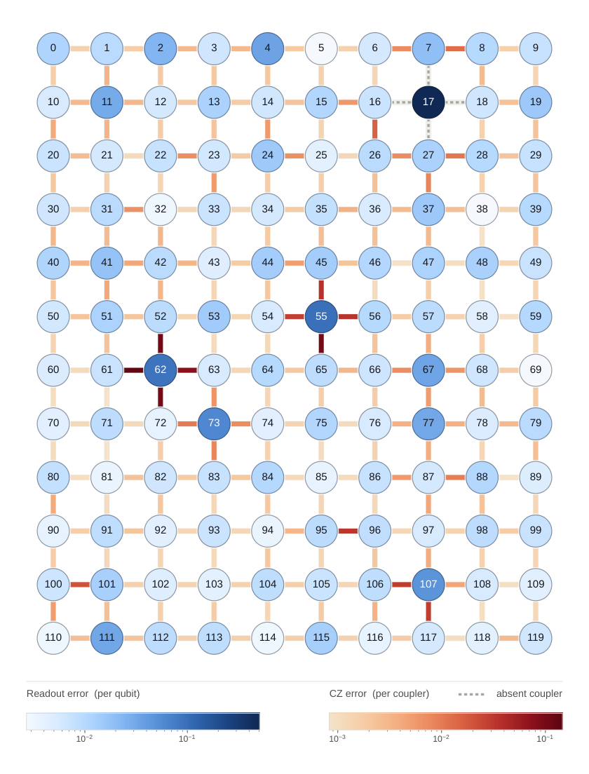
Hardware.—All experiments were performed on a 120-qubit superconducting QPU based on the Nighthawk architecture. We compare results for the first and the second iterations of this architecture (r1 vs r2). In contrast to the heavy-hexagon connectivity of the preceding IBM chips, Nighthawk arranges its qubits on a square lattice whose nearest-neighbor pairs are connected by tunable couplers, i.e. the full square-lattice connectivity is available with a total of 218 couplers. This connectivity makes it a natural fit for RCS experiments, which are traditionally performed on two-dimensional grids, allowing the circuit to be laid out on Nighthawk without any routing overhead. The native gate set consists of the two-qubit CZ gate together with one-qubit gates and . rotations are implemented virtually as frame updates and are therefore error-free and of zero duration [31]. The device also exposes gates, but we do not use them in our experiments, so every one-qubit gate compiles to two SX pulses and virtual RZs. At the time of our runs the device showed a median CZ error of , median SX error of around and a median readout assignment error of . An error map displaying the CZ and readout errors immediately before the experiment is shown in Fig. 1(a). Because single-qubit errors are one to two orders of magnitude below the CZ error and RZ is exact, the error budget of the circuits described below is dominated by the two-qubit layers and by readout, which motivates several of the methodological choices that follow.
Calibration-aware placement.—Rather than fixing the physical qubit subset by hand, we select it programmatically from the most recent calibration data immediately before each experiment. The target layout is a rectangular grid; every rigid offset of the logical grid inside the physical lattice is scored by a log-fidelity proxy built from the reported readout, SX, and CZ error rates, with missing couplers penalized like -error gates, and qubits or couplers failing per-element error thresholds dropped from the candidate (Appendix A). Among all candidates within a small slack of the optimal score, the one retaining the most qubits is selected. For the experiment described here, the search retained qubits (three qubits were dropped by the calibration filters) and 102 couplers between retained qubits, as shown in Fig. 1(b). All circuits below act on these qubits, and all gate layers are restricted to the 102 couplers that appear in the executed circuits.
Random circuit ensemble.—Our circuits follow the standard RCS construction of alternating one- and two-qubit layers [9, 4]. One cycle consists of (i) a layer of independent Haar-random SU(2) gates on every qubit, followed by (ii) a layer of CZ gates applied on a matching of the coupling graph. Haar-random one-qubit gates are sampled in the decomposition with and . The two-qubit layers cycle through the canonical four-coloring of the square-lattice edges, = (horizontal-even, horizontal-odd, vertical-even, vertical-odd), in the fixed repeating order . After the placement-driven pruning above the four matchings contain edges, i.e. CZ gates per cycle on average (1020 CZ gates at the deepest benchmarked point, cycles). A depth- circuit applies cycles and a terminal measurement of all qubits in the computational basis. Once built, the circuits are transpiled to the native gate set with a locked one-to-one layout onto the qubits selected above, without additional routing.
Patched circuits.—A direct verification through XEB is classically demanding at the scale we probe (Sec. III). Following the patch-verification methodology introduced previously [4, 32], we estimate the fidelity of circuits too large for full classical verification by running patched variants: the qubit set is partitioned into patches and all CZ gates crossing patch boundaries are removed, so the circuit factorizes into independent, classically simulable blocks. We benchmark patched families with .
A single fixed partition would tie the benchmark to one specific set of removed couplers and one specific set of subcircuit ensembles. To separate the fidelity estimate from any particular cut, we use randomized patching [Fig. 1(c)]: for every we take the five best partitions found by a cut-minimizing combinatorial optimizer (Appendix B) and allocate three random circuit instances to each, giving 15 independent circuits per data point. Instance-to-instance fluctuations then average over both the random gates and the choice of cut, and the quoted uncertainty includes the patching-induced spread.
For each patched circuit we compute the XEB patch-by-patch [9, 4]. Let , , be the measured bitstrings, their substrings corresponding to patch of qubits, and the ideal output distribution of patch (obtained by exact statevector simulation of the patch subcircuit). The per-patch estimator is then
| (1) |
where the denominator is the noiseless value of the numerator, evaluated from the same statevector [4]. For an anticoncentrated patch it equals and Eq. (1) reduces to the standard linear XEB; at shallower depth, where the patch output has not yet anticoncentrated, the normalization removes the corresponding upward bias (for our experiments patched circuits start to anticoncentrate around 24 cycles, see Appendix F). The total circuit fidelity is estimated as the product over patches
| (2) |
Ideal patch probabilities were computed with statevector simulation on the BlueQubit platform (CPU; patches of at most 21 qubits).
Mirror benchmark.—Patched XEB certifies the constituent patches but is, by construction, blind to errors on the removed boundary couplers, and any XEB-type estimate at these sizes relies on classical simulability of the reference distribution. As an independent, simulation-free consistency check we run a mirror benchmark [38], consisting of a state-preparation layer, a forward random circuit of cycles, its exact inverse , and a readout. The survival probability—the probability of recovering the prepared bitstring—is a direct fidelity estimate for the -cycle sequence and requires no simulation.
To make the mirror and patched curves comparable at fixed depth, we mirror a pseudo-patched circuit constructed to match the patched family gate-for-gate within while remaining connected: the forward circuit cycles through the five boundary-edge sets, omitting in each cycle only the currently active partition’s boundary gates, so that removed gates have patched-circuit multiplicity but every coupler is used again under a different partition (Appendix C). Coherent-error cancellation between the two mirror halves is suppressed by randomized compiling with 64 Pauli-frame randomizations per circuit [42, 23, 38], and readout-asymmetry bias is removed by preparing random Hamming-weight- input strings, 10 per circuit, matching the SPAM exposure of the anticoncentrated XEB outputs (Appendix C). For each mirror point we run 3 independent circuit instances, matching the per-partition instance count of the patched runs.
All fidelity curves and the -sample run were executed through Qiskit Runtime batch execution, interleaved at the level of individual depth points and measurement-twirled throughout, so that calibration drift affects all curves alike and cross-curve comparisons at fixed depth remain unbiased (Appendix D).
III Estimating the classical cost of sampling
Every number in this section traces to a stated convention and can be reproduced from the released circuits; the estimator itself is validated against the published advantage networks in Appendix E.
Task and conventions.—The task we cost is the one used in Refs. [32, 26, 16]: generate samples from a bounded-fidelity approximation to the ideal 61-qubit output distribution—one reproducing the experiment’s global fidelity —by frugal rejection sampling from tensor-network amplitude evaluations. In this strategy, drawing samples requires approximate output probabilities with [32], and the bounded-fidelity trick makes the work linear in [26]. Writing for the number of complex multiply–adds in a single amplitude contraction, the estimated work and runtime are
| (3) |
with the factor of converting one single-precision complex multiply–add to machine floating-point operations, and Frontier taken as the reference machine with theoretical peak FLOPS at sustained efficiency [5, 40], following the conventions of Refs. [32, 16].
This task is strictly stronger than producing bitstrings that merely match the experimental XEB score. Score-level spoofing algorithms attain the latter at far lower cost while carrying parametrically smaller fidelity: samples drawn from the product distribution of two severed halves that reach would have global fidelity of order [17, 2]. Equation (3) is therefore an algorithm-specific estimate for bounded-fidelity sampling of the full circuit, not a lower bound on the cost of matching the reported score; the three classical tasks—exact amplitude evaluation, bounded-fidelity sampling, and score spoofing—are separated quantitatively in Appendix E, and the margin against score spoofing is measured on our own circuit ensemble in Appendix F.
Two remarks on conventions, both consequential when comparing across papers. First, in Eq. (3) counts complex operations; published tables that fold the factor of into the displayed FLOP counts differ from arXiv-convention tables by exactly that factor.22 2 Both conventions appear in the literature for the same experiments; we verified by back-computing the stated runtimes that the arXiv version of Ref. [32] tabulates complex FLOPs while the published version tabulates machine FLOPs. All values quoted in this paper are complex FLOPs unless labeled “machine.” Second, Eq. (3) prices the probabilities as independent single amplitudes. This is the transparent baseline, but it is not what an optimized attack would do, and the corrections do not all point the same way: multi-amplitude and batched sparse-output contraction reuse intermediates across the evaluations and lower the cost [28, 16], while finite memory forces slicing and recomputation that raise it, by amounts that span many orders of magnitude on the published networks [32, 16]. We therefore quote Eq. (3) evaluated with unlimited-memory contraction paths and report the sensitivities separately below.
Estimator and search protocol.—Circuits are converted to tensor networks in quimb [21] and contraction orders are searched with the hyper-optimized protocol of cotengra [20]: graph-partitioning trials (KaHyPar) under Bayesian hyperparameter search, keeping the best contraction tree found. is the standard contraction cost of the best tree—the sum over pairwise contractions of the product of participating bond dimensions [29]—and the reported width is the base-2 logarithm of the largest intermediate tensor.
Path quality, not the cost formula, dominates the error of such estimates, so we state the search budgets explicitly. The validation networks of Appendix E were each searched for 5 hours on 128 cores per contraction mode. At small budgets the estimator is badly biased upward—minutes-scale single-core searches overestimate the converged values by two to five orders of magnitude on the same networks—and the bias shrinks with budget until the best-found cost plateaus. The experimental circuits of Table 1 were searched with the same protocol under depth-scaled time budgets, from two minutes at 8 cycles to 1.5 hours at 32–40 cycles on 20 parallel workers (– trials per circuit). Independent repeat searches at depths 32, 36, and 40 with 2.5-hour budgets agree with the first to , , and decades, which we take as the search scatter; since the depth-36 network contains the depth-32 network, the optimal is in fact bounded above by the depth-36 entry, and we quote each best-found value as is. All quoted costs remain upper bounds on the true optimal contraction cost.
Depth dependence for the experimental circuits.—Table 1 reports the converged single-amplitude cost for our 61-qubit circuit family at every measured depth.
| cycles | 2q gates | width | ||
|---|---|---|---|---|
| 4 | 102 | 1 | – | – |
| 8 | 204 | 11 | 5.09 | 3.2 s |
| 12 | 306 | 20 | 7.93 | 1.3 ms |
| 16 | 408 | 27 | 10.53 | 0.3 s |
| 20 | 510 | 34 | 12.95 | 44 s |
| 24 | 612 | 43 | 15.45 | 2.2 h |
| 28 | 714 | 49 | 17.58 | 7 d |
| 32 | 816 | 56 | 19.83 | 2 yr |
| 36 | 918 | 64 | 21.82 | 108 yr |
| 40 | 1020 | 65 | 22.03 | 99 yr |
Below the knee the cost grows by a nearly constant factor of per four cycles—exponential growth at roughly two width units per cycle—and at 36 cycles the width reaches and the growth stops: between depths 36 and 40 the cost changes by less than a factor of two. The measured knee position, between 32 and 36 cycles, matches the heuristic to within one four-cycle step. The coefficient is where the native gate set enters. CZ has operator Schmidt rank 2 and contributes one ebit per gate across a contraction cut, whereas the iSWAP-family gates of Refs. [4, 32, 16] have rank 4 and contribute two [4, 29]; correspondingly, the published networks saturate near while our CZ circuits require . A weaker entangler delays the crossover but does not lower the saturated cost, which is pinned at system size on either gate set.
At the anchor depth this cost is already far beyond direct verification: complex operations is 2 days of the full reference machine for a single amplitude, which is why the fidelity at 36 cycles is measured by mirror and patch estimators rather than by full-circuit XEB.
Sampling cost and sensitivity.— Combining Table 1 with the measured fidelities gives the headline estimates. At 36 cycles, (global-fit value, Table 1; measured –) and yield machine FLOPs, i.e. Frontier years at the stated efficiency. At 40 cycles the same formula with the fitted and gives years, and at 32 cycles (, ) only years: the contraction cost saturates between 32 and 36 cycles while the fidelity keeps decaying, so the fidelity-weighted work is maximized at the knee. This is the quantitative reason the 36-cycle point anchors our claim.
The sensitivities are as follows, and we state them rather than absorb them. (i) Fidelity: is linear in within this strategy; the linearity is a property of the bounded-fidelity algorithm, not of the task [26]. (ii) Memory model: we quote unlimited-memory paths; on the same published network, realistic-memory and unlimited-memory estimates differ by up to twelve orders of magnitude in Ref. [32], so the memory convention dominates every other choice, and quoting the floor is the conservative direction for an advantage claim. (iii) Path search: converged-budget searches are upper bounds on the optimal with residual scatter decades at saturation. (iv) Algorithm: Eq. (3) does not price multi-amplitude reuse [28], approximate contraction [19], finite-fidelity matrix-product simulation [6], or spoofing strategies that target the score rather than the distribution [17, 3]; any of these can reduce the effective cost, and the history of this benchmark says some will [27, 36, 45].
IV Discussion
We have run random-circuit sampling at the scale of the published advantage experiments on a publicly available QPU accessible through a cloud, using the code that we release with this paper. The full experiment—two fidelity estimators at every depth from 4 to 40 cycles plus the -sample run of the 61-qubit, 36-cycle circuit—consumed about 11 minutes of QPU execution time, of which the sampling run itself took 19 s (Appendix D). The two estimators, one simulation-free (the mirror benchmark) and one built on exact patch simulation, agree at every depth from 20 to 40 cycles. The second-generation IBM Nighthawk r2 is a large step beyond the r1, compounding to an order of magnitude fidelity difference at 32–40 cycles, while a reduced shot repetition delay allows runs that took several hours of QPU time on r1 to be executed within minutes on r2.
The directly supported point is the 61-qubit, 36-cycle experiment, at the knee of the contraction cost; the 40-cycle data show that both estimators keep following the same exponential past it, where, under the cost model of Sec. III, the classical task becomes slightly cheaper again. Score spoofing and noise-induced classical algorithms limit what any finite-fidelity RCS experiment can claim, and simulation methods keep getting faster [24, 27, 36, 45, 2, 7, 17, 3]; this is why we quote unlimited-memory cost floors rather than memory-constrained headline numbers. For the severing family specifically, Appendix F measures the attainable scores on our own ensemble: no branch reaches the 36-cycle score at all—the strongest falls a factor of ten short—so the family is excluded on score alone, without appeal to what it would cost to run. The analysis also leaves a concrete lesson for future placements: optimize graph expansion alongside gate fidelity.
Acknowledgments
We thank Petar Jurcevic for many fruitful discussions and acknowledge the use of IBM Quantum Credits via the IBM Quantum Startups Program for this work. The views expressed are those of the authors and do not reflect the official policy or position of IBM or the IBM Quantum Platform team.
Data and code availability
The data and code that support the findings of this work are openly available at https://github.com/BlueQubitDev/rcs-nighthawk. The repository contains all executed circuits—the mirror, patched, and full-circuit instances in QPY and OpenQASM 3 format, together with the qubit layout, the coupler four-coloring, the patch partitions, and the measured bitstrings, including the samples of the 36-cycle circuit. The code for circuit generation, calibration-aware placement, fidelity estimation, and contraction-cost estimation is also available.
Appendix A Placement details
For every possible offset of the logical grid inside the physical lattice ( candidate rectangles) we compute a log-fidelity proxy
| (4) |
where , and are the reported readout, SX and CZ error rates, the sums run over the qubits and grid edges of the candidate rectangle, and counts the missing edges, penalized at each (a missing edge is scored like a -error gate). Calibration data is absent for some edges, which we treat as missing and account for in the proxy. Within a candidate rectangle, qubits whose readout error exceeds are dropped, couplers whose CZ error exceeds are pruned, and any qubit left with no usable coupler is dropped as well. Among all candidates whose proxy fidelity is within a factor of the best one (a slack of in ), we select the one retaining the most qubits. This is a coarser, purpose-built variant of noise-aware layout selection in the spirit of mapomatic [34]: because the circuit family is translation-invariant on the grid, only a few rigid placements need to be scored.
Appendix B Patch generation
Patch partitions are produced by a randomized combinatorial optimizer operating on the 102-edge coupling graph, using boundary local search that moves single qubits between patches, subject to two constraints—every patch remains internally connected, and patch sizes stay balanced to within one qubit—while minimizing the number of cut edges. The optimizer returns the set of distinct optimal partitions found, ranked by cut size. For our experiment this yields for : qubits with 12–14 cut edges; for : qubits with 19–23 cut edges. Five partitions are retained at each .
These partitions are optimized for fidelity estimation (balanced, simulable patches), not for minimal boundary, and an adversary is not bound by the balance constraint. A randomized min-cut search over the same graph (Appendix F) gives, for cuts with both sides larger than 26 qubits, a minimum of 6 cut edges (a partition); relaxing the balance requirement further, an 11-qubit block detaches on 5 edges, a 4-qubit block on 3, and the graph carries eight degree-2 qubits that detach on 2. The gap between the balanced estimator partitions (12–23 cut edges) and these adversarial cuts (2–6) is what makes the score-spoofing analysis of Appendix F necessary: the estimator cuts are deliberately expensive to sever, while the cuts an attacker would actually choose are up to an order of magnitude cheaper.
Appendix C Mirror construction details
| experiment | cycles | 2q gate | published | ours | [Eq. (3)] | |||
|---|---|---|---|---|---|---|---|---|
| Sycamore-53 [4] | 53 | 20 | fSim | 17.78 | 18.40 | 14 d | ||
| Zuchongzhi-56 [44] | 56 | 20 | iSWAP-like | 19.78 | 19.44 | 45 d | ||
| Zuchongzhi-60 [46] | 60 | 24 | iSWAP-like | 21.00 | 20.85 | 1.6 yr | ||
| Sycamore-70 [32] | 70 | 24 | fSim | 23.70 | 23.00 | yr | ||
| Sycamore-67 [32] | 67 | 32 | fSim | 23.30 | 23.31 | yr | ||
| Zuchongzhi-3.0 [16] | 83 (of 105) | 32 | iSWAP-like | — | — | yr | ||
| this work (IBM Nighthawk r1) | 62 | 32 | CZ | — | 22.0 | — | 20 yr | |
| this work (IBM Nighthawk r2) | 61 | 36 | CZ | — | 21.8 | — | 110 yr | |
| cut | margin | ||
|---|---|---|---|
| balanced | 6 | – | |
| 11-qubit block | 5 | – | |
| pendant arms | 3 | ||
| adjacent pairs∗ | 4 | ||
| singletons∗ | 2 |
Pseudo-patched forward circuit.—A mirror of the full circuit would contain more two-qubit gates per cycle than the patched circuits it is compared against (the patched variants lack the boundary gates), so the two benchmarks would not be exactly comparable at fixed depth—their per-cycle error budgets would differ. The forward circuit therefore cycles through the same five boundary-edge sets used for randomized patching, advancing to the next partition every cycle; in each cycle, the CZ gates belonging to the currently active partition’s boundary are omitted from that cycle’s matching. Every removed gate is thus a genuine patch-boundary gate of one of the partitions and the number of omitted gates per four-cycle period matches a patched circuit. But because the active partition rotates, a coupler severed in one cycle is used again at its next appearance under a different partition, so the interaction graph of the forward circuit remains connected. The construction sits between the “patched” and “elided” verification circuits [4, 32]—gates are removed with patched-circuit multiplicity, but the circuit stays connected as in the elided variant—while additionally being mirrored. As a result the mirror curve and the patched curves can be plotted against either depth (cycles) or two-qubit gate count: the “cycle picture” and “gate-count picture” coincide on the -axis by construction.
Gate twirling.—Mirror circuits are vulnerable to coherent-error cancellation: systematic control errors in can partially undo those of , biasing survival probabilities optimistically relative to the error accumulated by a non-mirrored circuit. We suppress this with randomized compiling (gate twirling) [42, 23, 38]: each executed randomization dresses the two-qubit gate layers with independently sampled Pauli frames, with 64 randomizations per circuit, converting coherent errors into stochastic Pauli channels whose contributions add rather than cancel between the two mirror halves.
Input randomization.—Readout on superconducting devices is asymmetric: confusion-matrix calibrations on Nighthawk r2 QPU give a median misassignment of against . A mirror benchmark prepared on the all-zeros state would therefore see only the smaller error branch and would be biased high relative to the XEB curves, whose anticoncentrated output strings have a higher average Hamming weight and thus experience the symmetrized readout error per qubit. To make the comparison fair, we randomize the input to mirror circuits: the preparation layer applies on a uniformly random half of the qubits, giving random Hamming-weight- bitstrings. Each mirror circuit is executed on 10 random input strings with an equal share of the shot budget, and the survival probability is averaged over inputs. This makes the SPAM contribution of the mirror benchmark closer to that of the patched XEB curves.
Appendix D Execution schedule, drift mitigation, and measurement twirling
The full experiment—the mirror benchmark at 4–40 cycles, the and patched families at 20–40 cycles, and the -sample supremacy run of the unpatched 36-cycle circuit—was executed on ibm_phoenix through Qiskit Runtime batch execution, with shots in total and about 11 minutes of QPU execution time at the backend’s default shot repetition delay of s; the -sample supremacy run alone took 19 s.
Drift in gate and readout calibrations over minutes motivates the job order: if each curve were collected end-to-end before starting the next, slow drift would give every curve a different effective error rate and break the cross-curve comparisons at fixed depth that our analysis relies on. We therefore interleave the curves at the level of individual data points: the execution iterates over depths in ascending order and, at each depth, submits back-to-back one job per curve that includes that depth—first the mirror, then and . A patched job carries all 15 circuit instances of a data point (five partitions, three instances each) and a mirror job its instance–input combinations, so all curves sample any given calibration epoch at the same depths. Hardware drift then shows up as correlated fluctuations that make the individual curves somewhat bumpier, but relative comparisons between curves at fixed depth remain unbiased. Per-instance shot budgets grow with depth to track the shrinking fidelity signal, from to shots per patched circuit and from to per mirror instance. Fidelities are combined across instances using an inverse-variance weighted average.
For the same reason we enable measurement twirling on every job in the session. This symmetrizes the readout, so that slow drift in readout error cannot bias one curve relative to another depending on when it was collected, and it makes the readout-error contribution identical in kind across the mirror and XEB benchmarks. Gate twirling is applied to the mirror circuits only (Appendix C), since the XEB estimator is insensitive to the coherent-cancellation effect that motivates twirling in mirrored circuits.
Appendix E Validation of the contraction-cost estimator
The estimator was validated on the tensor-network graph files released with Google’s contraction-order optimizer [18], which specify the exact networks behind the single-amplitude column of Table 1 of Ref. [32]. Table 2 compares our best-found against the published values for all five circuits.
Agreement is within decades on all five networks and within decades on the deepest (Sycamore-67 at 32 cycles), which is the circuit most comparable in depth to our experiment. As an end-to-end check at larger scale, we also rebuilt a geometry-approximate Zuchongzhi-3.0 network (83 qubits, 32 cycles, iSWAP-type gates in the published ABCDCDBA schedule) and evaluated Eq. (3) at their reported : the resulting runtime is within a factor of four of the unlimited-memory estimate of Ref. [16] ( Frontier years), the appropriate comparison row for our memory convention. Because the exact qubit selection of that device is not public, we regard this as a consistency check rather than a reproduction.
Appendix F Severing attacks and placement on the weak-noise side
The linear XEB score can be attained by a dishonest classical spoofer without sampling from any bounded-fidelity approximation of the circuit. The relevant family is the severing attack [17, 7, 2]: partition the qubits into , delete the CZ gates crossing the cut, sample the severed parts independently, and submit the product samples. Whether such attacks succeed at a given operating point is a phase question—the measured score contains a global sector decaying with the full error budget and subsystem sectors decaying with a subsystem’s error budget plus a boundary penalty, and the competition between the two is the noise-induced transition of Refs. [32, 43]. Our ensemble, CZ entanglers with Haar-random SU(2) rotations, is the family for which severing is most effective: Ref. [17] reaches for a CZ ensemble on the Sycamore-53 geometry, versus of the experimental score for the actual fSim ensemble. We therefore quantify the margin on our own circuits rather than by transfer from published geometries. The attack scores below are properties of the ideal circuits and the coupler graph; device data enters only through the fidelity fit that sets the comparison target.
Setup.—For a cut severing couplers, each fired once per four-cycle color sweep, the attack score decays as , with the score fraction retained per severed CZ, while the global signal decays as , a factor per cycle [the fit of Fig. 2]. At the rate level a subsystem sector outruns the global signal iff its per-cycle attenuation is the weaker one, , with the per-qubit per-cycle error; at finite depth the prefactors compete with the accumulated decays, and for small the uniform- approximation itself fails (the effective decay of few-qubit marginals is governed by a size-dependent gap [17]). Rate margins alone therefore settle nothing for the small-subsystem modes; both and have to be measured, cut by cut.
Adversarial cuts of the realized coupler graph.—The partitions of Appendix B minimize cut size under a patch-balance constraint appropriate for fidelity estimation; an adversary is not so constrained. A randomized min-cut search over the realized 102-edge graph finds a balanced cut severing couplers, an 11-qubit block attached by , a 4-qubit block and a 3-qubit arm (qubits 5, 6, 14) each attached by , and eight degree-2 qubits ( singleton modes). All are low-expansion motifs, left because the placement optimizer sees only calibration data (Appendix A).
Exact attack scores on ensemble instances.—For targets restricted to -qubit regions of the coupler graph the attack score is an exact inner product of the target probability vector with the severed product distribution, free of sampling noise. Two practical points govern the measurement. First, the single-instance score of a small- mode fluctuates by from circuit to circuit, burying the deep-circuit mean; we therefore average 120 independently drawn instances of the ensemble (Haar SU(2) layers over the experiment’s color classes) in each of three regions centered on the weak motifs above, resolving means at the level. Second, the fitted decays are boundary-local: across region sizes and cut geometries the retained fraction is – per severed CZ with prefactors – and no systematic size trend, and at the per-instance speckle is , so the ensemble means measured here are the operative scores at full size.
The result is that no severing branch reaches the experimental score at the 36-cycle anchor (Table 3). At that depth every mode we can measure is consistent with zero: the singletons and adjacent pairs all fall within , and the strongest of them, a two-sided arm mode, reaches —itself from zero, and an order of magnitude below the target . Extrapolating the fitted rates to the wider cuts that an adversary would need for a balanced partition gives – for the 11-qubit block () and – for the balanced cut (); even the most attacker-favorable rate and prefactor in the measured band leave these six orders of magnitude below target.
Margin at the operating point.—Because every branch falls short on score, the severing family is excluded here without appeal to what it would cost to run—a stronger statement than was available for the first-generation device, where the two-sided pendant modes did reach the target score and had to be excluded by their sampling cost instead. The improvement is not a change in the graph, whose cut structure is comparable, but in the device: the r2 target score is an order of magnitude higher, while the attainable severed scores are set by the ideal circuits and are if anything smaller (measured – per severed CZ, against – on the r1 ensemble). Raising fidelity raises the bar a spoofer must clear without giving the spoofer anything. The same conclusion holds at the rate level and now with margin for every cut the graph admits, including the singleton modes that were marginal on r1: the boundary bill exceeds the noise saved by – for a degree-2 singleton and by – for the balanced cut. Known top- postprocessing improves severed scores by factors [17] and does not change the conclusion. These are attack-class-relative statements, on the same footing as the corresponding analyses of Refs. [32, 16].
Anticoncentration.—The same computation certifies the first crossover. The Porter–Thomas collision ratio reaches by 24 cycles, around by 32 cycles and remains there at 36 and 40 cycles, placing the anchor depth well inside the anticoncentrated regime and away from the shallow-circuit spoofing window of Refs. [7, 13].
Implication for placement.—The weak motifs above—an 11-qubit block on five edges, a 4-qubit block and a 3-qubit arm on three, eight degree-2 qubits—are all artifacts of a placement objective that optimizes calibration data alone (Appendix A). A placement that additionally penalizes low-conductance cuts, trading a small amount of median gate fidelity for graph expansion, would remove them and widen the margin further at essentially no cost in circuit fidelity; we regard this as a design rule for future experiments. The scaling caveat is set by geometry: at fixed per-gate error on a fixed-degree planar lattice the boundary bill of the best cut grows only as while the global error budget grows as , so at constant sufficiently large systems cross to the strong-noise side [43, 32, 3]; improved fidelity or connectivity moves the crossing outward, and the r1-to-r2 improvement is an instance of exactly that.
References
- [1] (2017) Complexity-theoretic foundations of quantum supremacy experiments. In Proceedings of the 32nd Computational Complexity Conference, LIPIcs, Vol. 79, pp. 22:1–22:67. External Links: Document Cited by: §I.
- [2] (2020) On the classical hardness of spoofing linear cross-entropy benchmarking. Theory of Computing 16 (11), pp. 1–8. External Links: Document Cited by: Appendix F, §I, §III, §IV.
- [3] (2023) A polynomial-time classical algorithm for noisy random circuit sampling. In Proceedings of the 55th Annual ACM Symposium on Theory of Computing, pp. 945–957. External Links: Document Cited by: Appendix F, §I, §III, §IV.
- [4] (2019) Quantum supremacy using a programmable superconducting processor. Nature 574, pp. 505–510. External Links: Document Cited by: Table 2, Appendix C, §I, §I, §II, §II, §II, §II, §III.
- [5] (2023) Frontier: exploring exascale. In Proceedings of the International Conference for High Performance Computing, Networking, Storage and Analysis (SC ’23), pp. 1–16. External Links: Document Cited by: §I, §III.
- [6] (2023) Density-matrix renormalization group algorithm for simulating quantum circuits with a finite fidelity. PRX Quantum 4, pp. 020304. External Links: Document Cited by: §I, §III.
- [7] (2021) Spoofing linear cross-entropy benchmarking in shallow quantum circuits. In 12th Innovations in Theoretical Computer Science Conference (ITCS 2021), LIPIcs, Vol. 185, pp. 30:1–30:20. External Links: Document Cited by: Appendix F, Appendix F, §I, §IV.
- [8] (2017) Simulation of low-depth quantum circuits as complex undirected graphical models. Note: arXiv:1712.05384 Cited by: §I, §I.
- [9] (2018) Characterizing quantum supremacy in near-term devices. Nature Physics 14, pp. 595–600. External Links: Document Cited by: §I, §II, §II.
- [10] (2022) Noise and the frontier of quantum supremacy. In 2021 IEEE 62nd Annual Symposium on Foundations of Computer Science (FOCS), pp. 1308–1317. External Links: Document Cited by: §I.
- [11] (2019) On the complexity and verification of quantum random circuit sampling. Nature Physics 15, pp. 159–163. External Links: Document Cited by: §I.
- [12] (2018) Classical simulation of intermediate-size quantum circuits. Note: arXiv:1805.01450 Cited by: §I.
- [13] (2022) Random quantum circuits anticoncentrate in log depth. PRX Quantum 3, pp. 010333. External Links: Document Cited by: Appendix F, §I.
- [14] (2024) Random quantum circuits transform local noise into global white noise. Communications in Mathematical Physics 405, pp. 78. External Links: Document Cited by: §I.
- [15] (2025) Computational power of random quantum circuits in arbitrary geometries. Physical Review X 15, pp. 021052. External Links: Document Cited by: §I.
- [16] (2025) Establishing a new benchmark in quantum computational advantage with 105-qubit Zuchongzhi 3.0 processor. Physical Review Letters 134, pp. 090601. External Links: Document Cited by: Table 2, Appendix E, Appendix F, §I, §I, §I, §III, §III, §III, §III.
- [17] (2024) Limitations of linear cross-entropy as a measure for quantum advantage. PRX Quantum 5, pp. 010334. External Links: Document Cited by: Appendix F, Appendix F, Appendix F, §I, §III, §III, §IV.
- [18] (2024) rcs_tnsa: simulated-annealing contraction-order optimization for random circuit sampling. Note: https://github.com/google-research/google-research/tree/master/rcs_tnsa Cited by: Table 2, Appendix E.
- [19] (2024) Hyper-optimized approximate contraction of tensor networks with arbitrary geometry. Physical Review X 14, pp. 011009. External Links: Document Cited by: §I, §III.
- [20] (2021) Hyper-optimized tensor network contraction. Quantum 5, pp. 410. External Links: Document Cited by: §I, §I, §III.
- [21] (2018) Quimb: a python package for quantum information and many-body calculations. Journal of Open Source Software 3 (29), pp. 819. External Links: Document Cited by: §III.
- [22] (2023) Computational advantage of quantum random sampling. Reviews of Modern Physics 95, pp. 035001. External Links: Document Cited by: §I.
- [23] (2021) Randomized compiling for scalable quantum computing on a noisy superconducting quantum processor. Phys. Rev. X 11 (4), pp. 041039. External Links: Document Cited by: Appendix C, §II.
- [24] (2020) Classical simulation of quantum supremacy circuits. Note: arXiv:2005.06787 Cited by: §I, §IV.
- [25] (2024) Quantum computing with Qiskit. Note: arXiv:2405.08810 Cited by: §I.
- [26] (2021) Classical sampling of random quantum circuits with bounded fidelity. Note: arXiv:2112.15083 Cited by: §I, §I, §III, §III.
- [27] (2021) Closing the “quantum supremacy” gap: achieving real-time simulation of a random quantum circuit using a new Sunway supercomputer. In Proceedings of the International Conference for High Performance Computing, Networking, Storage and Analysis (SC ’21), External Links: Document Cited by: §I, §III, §IV.
- [28] (2024) Verifying quantum advantage experiments with multiple-amplitude tensor-network contraction. Physical Review Letters 132, pp. 030601. External Links: Document Cited by: §I, §I, §III, §III.
- [29] (2008) Simulating quantum computation by contracting tensor networks. SIAM Journal on Computing 38 (3), pp. 963–981. External Links: Document Cited by: §I, §I, §III, §III.
- [30] (2021) Theory of mirror benchmarking and demonstration on a quantum computer. Note: arXiv:2108.10431 Cited by: §I.
- [31] (2017) Efficient Z gates for quantum computing. Phys. Rev. A 96 (2), pp. 022330. External Links: Document Cited by: §II.
- [32] (2024) Phase transitions in random circuit sampling. Nature 634, pp. 328–333. External Links: Document Cited by: Table 2, Table 2, Table 2, Appendix C, Appendix E, Appendix F, Appendix F, Appendix F, §I, §I, §I, §II, §III, §III, §III, §III, §III, footnote 2.
- [33] (2023) The hardness of random quantum circuits. Nature Physics 19, pp. 1719–1724. External Links: Document Cited by: §I.
- [34] (2023) Suppressing quantum circuit errors due to system variability. PRX Quantum 4 (1), pp. 010327. External Links: Document Cited by: Appendix A.
- [35] (2018) A blueprint for demonstrating quantum supremacy with superconducting qubits. Science 360, pp. 195–199. External Links: Document Cited by: §I.
- [36] (2022) Solving the sampling problem of the Sycamore quantum circuits. Physical Review Letters 129, pp. 090502. External Links: Document Cited by: §I, §III, §IV.
- [37] (2018) Quantum computing in the NISQ era and beyond. Quantum 2, pp. 79. External Links: Document Cited by: §I.
- [38] (2022) Measuring the capabilities of quantum computers. Nat. Phys. 18 (1), pp. 75–79. External Links: Document Cited by: Appendix C, §II, §II.
- [39] (2022) Scalable randomized benchmarking of quantum computers using mirror circuits. Physical Review Letters 129, pp. 150502. External Links: Document Cited by: §I.
- [40] (2026) Frontier — HPE Cray EX235a, AMD EPYC, AMD Instinct MI250X, Slingshot-11. Note: https://top500.org/system/180047/Accessed 22 July 2026 Cited by: §I, §III.
- [41] (2019) A flexible high-performance simulator for verifying and benchmarking quantum circuits implemented on real hardware. npj Quantum Information 5, pp. 86. External Links: Document Cited by: §I.
- [42] (2016) Noise tailoring for scalable quantum computation via randomized compiling. Phys. Rev. A 94 (5), pp. 052325. External Links: Document Cited by: Appendix C, §II.
- [43] (2023) A sharp phase transition in linear cross-entropy benchmarking. Note: arXiv:2305.04954 Cited by: Appendix F, Appendix F, §I.
- [44] (2021) Strong quantum computational advantage using a superconducting quantum processor. Physical Review Letters 127, pp. 180501. External Links: Document Cited by: Table 2, §I.
- [45] (2025) Leapfrogging Sycamore: harnessing 1432 GPUs for faster quantum random circuit sampling. National Science Review 12 (3), pp. nwae317. External Links: Document Cited by: §I, §III, §IV.
- [46] (2022) Quantum computational advantage via 60-qubit 24-cycle random circuit sampling. Science Bulletin 67 (3), pp. 240–245. External Links: Document Cited by: Table 2, §I.
- [47] (2023) Boundaries of quantum supremacy via random circuit sampling. npj Quantum Information 9, pp. 36. External Links: Document Cited by: §I.