Mapping the Milky Way in Six Dimensions: A contiguous, homogenised, phase-space catalogue of Gaia DR3 tracers up to 250 kpc.

Sutirtha Mukherjee ^, ^, ^†^†thanks: E-mail: sutirtham@tifrh.res.in Affiliation: Department of Theoretical Physics, Tata Institute of Fundamental Research, Mumbai Affiliation: Tata Institute of Fundamental Research, Hyderabad Amogh Srivastav ^, ^†^†thanks: E-mail: 23b1826@iitb.ac.in Affiliation: Department of Physics, Indian Institute of Technology Bombay Subhabrata Majumdar^, ^†^†thanks: E-mail: subha@tifr.res.in Affiliation: Department of Theoretical Physics, Tata Institute of Fundamental Research, Mumbai

Abstract

We present a comprehensive, quality-assured, homogenised catalogue of $32{,}552{,}876$ stellar sources with full 6D phase-space information, spanning a contiguous range of Galactocentric distances from the inner galaxy ( $\gtrsim 5$ kpc) to the outer halo ( $\sim\!250$ kpc). The catalogue cross-matches Gaia DR3 astrometry with spectrophotometric distances and line-of-sight velocities from 14 large-scale surveys (including desi, sdss-boss, apogee, lamost, galah, and ges). We achieve a median fractional distance uncertainty of $\approx 2.7\%$ for tracers with heliocentric distances, $d_{\rm helio}\leq 15$ kpc, increasing to $\approx 29\%$ for $15<d_{\rm helio}\leq 250$ kpc. The catalogue-wide median fractional radial velocity uncertainty is $\approx 8.31\%$ . Gaia-anchored, survey-specific zero-point corrections and statistical normalisation suppress both random and systematic errors before aggregation. We further derive spectrophotometric parallaxes by jointly exploiting multi-band photometry and spectroscopic observations. For sources with discrepant or missing measurements, superior data from overlapping surveys supersede unreliable values and supplement absent radial velocities, improving both completeness and internal consistency. This multi-survey synthesis yields precise parameters and kinematics for confirmed members of globular clusters, dwarf galaxies, and stellar streams when validated with external catalogues. Of the final sample, $517{,}123$ halo stars, predominantly faint ( $G>17$ ) and metal-poor ( $[\mathrm{Fe/H}]<-1$ ) tracers including RR Lyrae, blue horizontal-branch, and K giant stars, extend well beyond the Gaia parallax limit ( $\gtrsim\!10$ kpc), making this the largest, well-calibrated, statistical sample of halo tracers. This unique dataset is ideally suited for accurate multi-component mass modelling, cluster kinematics, chemical abundance mapping, galactic archaeology, dark matter searches, etc. over almost the entire Milky Way volume.

1 Introduction

Over the past two decades, there has been substantial advancement in stellar astrophysics, galactic kinematics and dynamics, and galactic archaeology, facilitated largely by the arrival of extensive large-scale digital surveys spanning photometric, astrometric, and spectroscopic domains. Early photometric surveys such as 2MASS (Skrutskie and others 2006), SDSS (York and others 2000), and Pan-STARRS (Chambers and others 2016) established the first wide-area maps of stellar density and colour across the Galaxy, while the Gaia space mission (Gaia Collaboration et al. 2016) has since delivered high-precision proper motions and parallaxes for $\sim$ 1.5 billion sources (Collaboration and others 2023; Gaia Collaboration et al. 2021), radial velocities for $\sim$ 33 million stars from its Radial Velocity Spectrometer (Katz and others 2019; Katz and others 2023), and BP/RP spectrophotometry for $\sim$ 220 million objects (Angeli and others 2023). Complementing Gaia’s astrometry, ground-based spectroscopic campaigns, including SEGUE (Yanny and others 2009; Rockosi and others 2022), LAMOST (Zhao et al. 2012; Luo and others 2016; Xiang and others 2019), GALAH (De Silva and others 2015), APOGEE (Majewski and others 2017), the Gaia-ESO Survey (Gilmore and others 2012), RAVE (Steinmetz and others 2006; Kordopatis and others 2013), and the Dark Energy Spectroscopic Instrument (DESI) Milky Way Survey (Cooper and others 2023; Collaboration 2023; Koposov and others 2024; Li and others 2025) now provide radial velocities, stellar atmospheric parameters, and chemical abundances for millions of stars across diverse Galactic environments.

The integration of radial velocities with astrometric proper motions and distances yields complete six-dimensional (6D) phase-space coordinates essential for identifying ancient accretion debris in integral-of-motion space (Myeong et al. 2018; Koppelman et al. 2019; Naidu and others 2020), determining the Milky Way’s mass distribution to its virial radius (Xue and others 2008; Deason and others 2021; Bird and others 2022; Koposov and et al. 2023), characterising the stellar halo density profile and shape (Deason et al. 2011; Deason et al. 2015; Sesar et al. 2010b; Pila-Díez and others 2015; Amarante et al. 2024), and mapping tidal streams and satellite kinematics (Vasiliev et al. 2021; Belokurov and Koposov 2016; Li and others 2019). The principal halo tracers employed for these studies, namely blue horizontal branch (BHB) stars (Xue and others 2008; Deason et al. 2011; Das and Binney 2016; Amarante et al. 2024), K giants (Xue and others 2014b; Xu and et al. 2018), near-main-sequence turnoff (nMSTO) stars (Sesar et al. 2010a; Jurić and others 2008; Željko Ivezić and others 2008), and RR Lyrae as well as other variable stars (Watkins and others 2009; Liu and others 2020; Cohen and others 2017; Feng and others 2024; Hernitschek and others 2017; Clementini and others 2019), each offer complementary advantages but also characteristic limitations: BHB stars are intrinsically rare and challenging to separate from blue stragglers; K giant luminosities span two orders of magnitude depending on age and metallicity, complicating distance inference; and nMSTO stars are too faint to probe $d\gtrsim 20$ kpc.

Table 1: Frequently used abbreviations and acronyms in this paper.

Abbrev.	Meaning	Abbrev.	Meaning	Abbrev.	Meaning
2MASS	Two Micron All Sky Survey	6D	Six-dim. phase space (3 pos. + 3 vel.)	AGB	Asymptotic Giant Branch
AGN	Active Galactic Nucleus	APOGEE	Apache Point Obs. Gal. Evol. Exp.	BHB	Blue Horizontal Branch
BOSS	Baryon Osc. Spectroscopic Survey	BP/RP	Blue/Red Photometer (Gaia)	CatWISE	WISE-based IR source catalogue
CMD	Colour–Magnitude Diagram	DESI	Dark Energy Spectroscopic Instrument	DR	Data Release
EM	Expectation–Maximisation	EMP	Extremely Metal-Poor	GALAH	Gal. Archaeology with HERMES
GCVS	Gen. Cat. of Variable Stars	GES	Gaia-ESO Survey	HB	Horizontal Branch
HEALPix	Hier. Equal Area isoLat. Pixelization	KG	K giant	LAMOST	Large Sky Area MOS Telescope
LEGUE	LAMOST Exp. for Gal. Und. & Expl.	LMC	Large Magellanic Cloud	LONEOS	Lowell Obs. Near-Earth-Object Search
MIST	MESA Isochrones & Stellar Tracks	MWS	Milky Way Survey	NGVS	Next Generation Virgo Survey
nMSTO	Near-Main-Sequence Turnoff	NSIDE	HEALPix resolution parameter	NSVS	Northern Sky Variability Survey
PARSEC	Padova–Trieste Stellar Evol. Code	PDR1	Pristine Data Release 1	PGS	Pristine-Gaia Survey
PL/PLZ	Period–Luminosity (–Metallicity)	PS1	Pan-STARRS1	PSF	Point Spread Function
PTR	Palomar Transient Factory RRL sample	QSO	Quasi-Stellar Object	RAVE	Radial Velocity Experiment
RC	Red Clump	RGB	Red Giant Branch	RRL	RR Lyrae
RRab/RRc	Fundamental/first-overtone RRL	RUWE	Renorm. Unit Weight Error	RVS	Radial Velocity Spectrometer
SDSS	Sloan Digital Sky Survey	SEGUE	Sloan Ext. for Gal. Und. & Expl.	Sgr	Sagittarius
SMC	Small Magellanic Cloud	SoS / SoS-I	Survey of Surveys (I)	SX Phe	SX Phoenicis stars
TOPCAT	Tool for Ops. on Cat. & Tables	UMP	Ultra Metal-Poor	VAC	Value-Added Catalogue
VMP	Very Metal-Poor	WISE	Wide-field IR Survey Explorer	XP	Gaia low-res. XP spectra
BIC	Bayesian Information Criterion	DUP	duplicate/repeated-measurement calibration route	TCH	three-cornered-hat method
GSR	Galactic Standard of Rest	LSR	Local Standard of Rest	KDE	kernel-density estimate

Table 2: Frequently used symbols and variables in this paper.

Symbol	Meaning	Symbol	Meaning	Symbol	Meaning
$\varpi$	Measured parallax	$\varpi_{c}$	Zero-point-corrected parallax	$Z_{\mathrm{EDR3}}$	Gaia EDR3 plx. zero-point corr.
$\sigma_{\varpi}$	Parallax uncertainty	$\sigma_{\mathrm{sys}}$	Systematic parallax floor	$\varpi_{\mathrm{est}}$	Model-predicted parallax
$\varpi_{\mathrm{phot}}$	Spectrophotometric parallax
$d$	Generic distance	$d_{\rm helio}$	Heliocentric distance	$d_{\rm plx}$	Parallax-based distance
$d_{\rm spec}$	Spectroscopic distance	$d_{\rm phot}$	Photometric distance	$d_{\rm phot}$	Spectrophotometric distance
$d_{\rm ref}$	Reference distance	$\sigma_{d_{\rm ref}}$	Uncertainty in $d_{\rm ref}$
$r_{\rm gc}$	Galactocentric radius	$R$	Galactocentric / cylindrical radius	$R_{xy}$	Cylindrical Galactocentric radius
$R_{\odot}$	Solar Galactocentric distance	$z$	Height above Galactic plane	$l,b$	Galactic longitude, latitude
$\mu_{\alpha^{*}}$	PM in RA ( $\times\cos\delta$ )	$\mu_{\delta}$	PM in declination	$\bm{\mu}$	Proper-motion vector
$\mathbf{C}_{\mu}$	PM covariance matrix
$G$	Gaia broad-band mag.	$G_{\rm BP},G_{\rm RP}$	Gaia BP/RP magnitudes	$C^{*}$	Corrected BP/RP excess
$A_{G}$	Extinction in Gaia $G$	$E(B\!-\!V)$	Reddening / colour excess	$E$	phot_bp_rp_excess_factor
$M_{G}$	Abs. mag. in Gaia $G$	$M_{V}$	Abs. mag. in Johnson $V$	$M_{R}$	Abs. mag. in $R$ band
$M_{W1}$	Abs. mag. in WISE $W1$	$M_{i^{\prime}}$	Abs. mag. in $i^{\prime}$ band	$M_{g}^{\rm BHB}$	BHB abs. mag. in SDSS $g$
$T_{\rm eff}$	Effective temperature	$T_{\rm eff}^{\rm Ref}$	Reference $T_{\rm eff}$ (RC cut)	$\log g$	Log surface gravity
$[\mathrm{Fe/H}]$	Iron metallicity (Solar ref.)	$[\alpha/\mathrm{Fe}]$	Alpha-element abundance	$Z$	Metal mass fraction
$P$	Pulsation period	$P_{F}$	Fundamentalised period	$\Phi$	Pulsation phase
$v_{r}$	Radial velocity	$\sigma_{v_{r}}$	RV uncertainty	$\Delta v_{r}$	Calibrated $-$ reference RV diff.
$V_{\rm helio}$	Heliocentric RV	$V_{\rm los}$	Line-of-sight velocity (GSR)	$V_{\rm LSR}$	LSR circular speed
$(U,V,W)$	Solar motion w.r.t. LSR
${\bf A}$	Design matrix (sp.phot. model)	${\bm{\theta}}$	Coefficient vector	$\lambda_{j}$	Regularisation hyperparameter
$y(\lambda)$	Sérsic-profile line model	$a,b,c$	Sérsic fit parameters	$\lambda_{0}$	Central wavelength
$N$	Total catalogue entries	$N_{\star}$	Unique stars after dedup.	$n$	Sigma-threshold parameter
$\eta$	Core / member fraction	$\langle P\rangle$	Mean purity	$x_{\rm cut}$	Generic quality threshold
$\Pi_{\rm RC}(x)$	Polynomial / purity function	$\mathcal{C}(x_{\rm cut})$	Completeness vs. threshold	$\mathcal{P}(x_{\rm cut})$	Purity vs. threshold
$\mathcal{Q}(x_{\rm cut})$	Simple quality function	$\mathcal{Q}_{\beta}(x_{\rm cut})$	Compl.–purity utility ( $\beta$ -weighted)	$\beta$	Compl./purity weight
$u$	Astrometric quality stat.	$\chi^{2}$	Chi-squared statistic	$\nu$	Degrees of freedom / $N_{\rm obs}$
$q_{d}$	Relative distance error	$q_{v}$	Relative RV error	$\mathrm{MAD}$	Median absolute deviation
$\tilde{d}$	Median recovered distance	$\tilde{d}_{\varpi}$	Median plx.-inferred distance	$\tilde{v}_{r}$	Median recovered RV
$P_{\mathrm{mem},i}^{(t)}$	Posterior membership prob.	$p_{\mathrm{mem}}^{(t)}$	Member spatial term	$p_{\mathrm{field}}^{(t)}$	Field spatial term
$\mathcal{L}_{\mathrm{mem},i}^{(t)}$	Member likelihood	$\mathcal{L}_{\mathrm{field},i}^{(t)}$	Field likelihood	$n_{\mathrm{ok}}$	Valid stars in EM update
$\mathcal{S}_{\mathrm{ok}}$	Valid-star set (EM)	$\bm{\mu}_{\mathrm{mem}}$	Member PM centroid	$w_{i}^{(t)}$	EM weight for star $i$
$v_{\mathrm{sys,EM}}$	Systemic velocity (EM)
$f_{\rm DUP}$	DUP RV scale factor	$f_{\rm tch}$	TCH RV scale factor	$f_{\star}$	Adopted RV norm. factor
$C$	Colour var. (Pristine dwarf–giant)	$grz$	Combined colour index (BHB sel.)

However, assembling a complete 6D sample from the solar neighbourhood to the outer halo ( $d\gtrsim 50$ kpc) remains a formidable challenge owing to two fundamental barriers. First, Gaia’s geometric parallaxes become unreliable beyond $\sim$ 5–10 kpc as fractional uncertainties exceed unity (Lindegren and others 2021; Bailer-Jones et al. 2021; Bailer-Jones 2023), a regime we term the “Gaia barrier,” where simple parallax inversion is dominated by noise and the Lutz–Kelker bias (Bailer-Jones et al. 2021). Second, the Gaia RVS is magnitude-limited to $G\lesssim 14$ (Katz and others 2023), leaving the vast majority of faint halo tracers without radial velocities. Existing outer-halo studies have consequently been forced to rely on small, heterogeneous samples of a few hundred to a few thousand tracers with full 6D information (Cohen and others 2017; Feng and others 2024; Xue and others 2011), or to work with incomplete phase-space coordinates.

Significant progress has been made on both fronts individually. For distances, spectrophotometric methods now achieve $\sim$ 10–25% precision through Bayesian isochrone fitting (Burnett and Binney 2010; Burnett and others 2011; Binney and others 2014; Xue and others 2014b; Carlin and others 2015; Das and Sanders 2019; Queiroz and others 2018; Queiroz and others 2020; Anders and others 2022; Yang and others 2025; Li and others 2025), data-driven models applied to Gaia XP spectra (Zhang et al. 2023b; Andrae et al. 2023; Ting et al. 2019; Xiang and others 2021; Xiang and others 2022), and the SpecDis neural-network catalogue for $>$ 4 million DESI stars (Li and others 2025), while the BOSS-HALO MINESweeper survey (Chandra and others 2025) extends Bayesian distances to $\sim$ 100 kpc for metal-poor halo giants. Period–luminosity–metallicity relations deliver $\sim$ 5% precision for RR Lyrae (Muraveva et al. 2015; Muraveva et al. 2018; Sollima et al. 2006; Braga et al. 2015) and Cepheids (Madore and Freedman 1991; Matsunaga et al. 2006), with Mira variables (Whitelock et al. 2008; Feast and Whitelock 2000; Soszyński and others 2007) and $\delta$ Scuti stars (McNamara 2011; McNamara 1997) extending the ladder to complementary populations. For radial velocities, the Survey of Surveys (Tsantaki and others 2022, SoS;) established the standard homogenisation framework by merging $\sim$ 11 million RV measurements from five surveys onto a common Gaia reference frame. More recently, Verberne et al. (2024) derived radial velocities from Gaia BP/RP spectra for $\sim$ 125 million sources ( $G<17.65$ ), and DESI provides $\sim$ 1 km s^-1 precision RVs for millions of stars through its MWS value-added catalogue (Koposov and others 2024). For each contributing survey, stars in common with Gaia define the radial-velocity calibration sample. Survey-dependent RV offsets and smooth trends with the available stellar/observational parameters are fitted on this overlap and then applied to place the survey velocities on the common Gaia RV scale.

Existing catalogues address complementary but distinct parts of this problem. SoS-I (Tsantaki and others 2022) homogenised radial velocities from Gaia, APOGEE, GALAH, Gaia-ESO, RAVE, and LAMOST onto a common scale for nearly 11 million stars, with reported zero-point accuracies of $\sim 0.16$ – $0.31\,\mathrm{km\,s^{-1}}$ . SoS-II (Turchi et al. 2025) extends the survey-combination philosophy to $T_{\rm eff}$ , $\log g$ , and $[\mathrm{Fe/H}]$ , using a PASTEL-calibrated spectroscopic reference and machine-learning estimates to provide atmospheric parameters for $\sim 23$ million stars. Our catalogue is complementary: its principal aim is a homogenised 6D phase-space sample that combines Gaia DR3 astrometry with DESI, other spectroscopic surveys, photometric information, and specialised halo tracers over $\sim 3$ – $250\,\mathrm{kpc}$ . Atmospheric parameters from SoS-II can be incorporated in future releases where available without changing the broader phase-space and outer-halo scope of the present catalogue. SpecDis delivers accurate spectrophotometric distances but only for DESI targets (Li and others 2025); Gaia XP catalogues offer large, parallax-calibrated distance samples yet lack homogenised radial velocities, since Gaia RVS covers only $\sim 33$ million bright stars (Zhang et al. 2023b; Andrae et al. 2023; Katz and others 2023); and dedicated outer-halo tracer studies remain limited to at most a few thousand stars with non-uniform error properties (Cohen and others 2017; Feng and others 2024; Liu and others 2020; Xue and others 2014b; Amarante et al. 2024; Xue and others 2011). The most complete existing combination, the DESI DR1 $\times$ Gaia DR3 cross-match (Koposov and others 2024)¹¹ 1 The official Gaia cross-match identifies the most probable Gaia counterpart of a source in an external catalogue through a local source-to-source procedure, in which nearby candidates are ranked using angular separation and the local source density. Our catalogue construction instead solves the distinct many-to-many survey problem of grouping repeated detections across heterogeneous survey products into one physical star. For catalogues already tied to dense reference catalogues such as Gaia, we adopt direct source_id matches, while specialised tracer catalogues and external systems are validated using the physical-parameter likelihood framework of Section 9., provides internally consistent radial velocities and spectrophotometric distances for $\sim 4$ million stars, but remains confined to the DESI footprint and target classes, does not extend beyond $\sim 100$ kpc, and offers no homogenisation framework for non-DESI surveys. Consequently, applications requiring large-scale, internally consistent 6D kinematics, including mass modelling, stream dynamics (Vasiliev et al. 2021), cluster kinematics, and substructure identification, still rely on ad hoc combinations of heterogeneous surveys that target distinct Galactic regions using different instrumentation and pipelines. Unifying these demands reconciling distance estimates that operate in fundamentally different precision regimes with distinct systematic sources: astrometric, spectrophotometric, photometric, and period-luminosity distances cannot be directly homogenised. It also requires propagating astrometric quantities to a common epoch, enforcing a consistent coordinate framework, carefully propagating uncertainties, rejecting outliers, and externally validating the catalogue before robust scientific inferences can be drawn.

In this paper, we address this gap by presenting a unified catalogue of $\sim$ 32.5 million unique Milky Way stars with complete 6D phase-space information, constructed by cross-matching, calibrating, deduplicating, and statistically aggregating 52 million input entries from 14 large-scale surveys spanning heliocentric distances from $\sim$ 3 kpc to $\sim$ 250 kpc, including $\sim$ 517,000 halo stars ( $R_{xy}>25$ kpc or $|z|>5\,\mathrm{kpc}$ ). Three principal methodological contributions distinguish this work. The first is a scalable cross-survey deduplication pipeline combining HEALPix spatial partitioning (NSIDE $\,=\,$ 32), $k$ -d tree pair-finding on unit-sphere Cartesian coordinates with parallax-consistency validation, and Union-Find connected-component extraction, achieving a 37.5% deduplication rate ( $N_{\star}=32{,}552{,}876$ unique stars) with inverse-variance weighted aggregation and outlier rejection. The second is an extended radial-velocity homogenisation framework that builds upon the SoS methodology of Tsantaki and others (2022) to encompass DESI and 15 additional catalogues not in the original SoS, deriving per-survey error normalisation and removing parameter-dependent zero-point offsets through weighted least-squares polynomial fitting against Gaia, reducing inter-survey systematics to $\lesssim$ 0.1–0.5 km s^-1. The third is a seven-term Bayesian expectation-maximisation membership framework applied to 1,722 discrete stellar systems: 189 globular clusters (Baumgardt and Vasiliev 2021), 1,481 open clusters (Cantat-Gaudin et al. 2018; Cantat-Gaudin et al. 2019; Cantat-Gaudin et al. 2020; Castro-Ginard et al. 2020; Soubiran et al. 2018), and 52 dwarf galaxies (Pace and others 2022; Koposov et al. 2011; Mateo et al. 2008; Geha et al. 2026), together with the Sagittarius stream (Vasiliev et al. 2021), jointly fitting spatial position, proper motion, radial velocity, spectrophotometric distance, CMD location, [Fe/H], and $\log g$ so that the most informative observable at each heliocentric distance automatically dominates the membership decision.

The construction is guided by a simple observational fact: no single distance or radial-velocity channel is uniformly reliable across the full Galactic volume. At small heliocentric distance, high-significance Gaia parallaxes provide the most direct distance information. As parallax precision deteriorates, we instead use spectrophotometric distances, inferred by combining spectroscopy with broad-band photometry and stellar models or data-driven calibrations, and specialised photometric distance relations for tracers such as BHB stars and RR Lyrae. Radial velocities are taken from Gaia and ground-based spectroscopic surveys, but their quoted uncertainties and zero points are first placed on a common scale. The catalogue therefore does not force one estimator to work everywhere; it selects and combines the most informative measurements available for each star while retaining provenance and uncertainty information.

The paper is organised as follows. Section 2 describes the input surveys, common quality cuts, and the parallax-based, spectrophotometric, photometric, and radial-velocity channels. The construction of the spectrophotometric distance estimator and its validation are described in the corresponding distance-method section. Section 3 then explains error normalisation, duplicate identification, RV zero-point calibration, and the final aggregation into one record per physical star. Section 9 tests the resulting catalogue against literature-based globular clusters, open clusters, dwarf galaxies, and the Sagittarius stream. Finally, Section C quantifies the retained-fraction–purity trade-off and Section 10 gives practical recommendations for science use.

Refer to caption — Figure 1: Sky coverage of the main components of the unified stellar catalogue in Galactic coordinates, shown in a Mollweide equal-area projection. Each panel shows a HEALPix density map with logarithmic colour scaling in stars per pixel. Shown are DESI DR1 SpecDist, Gaia 125M+33M (unique), LAMOST, Gaia SoS-I (unique), RAVE, SDSS/BOSS/SEGUE, and the final filtered catalogue. The Gaia-only unique panels isolate sources without external-survey counterparts. M31, the LMC, and the SMC are marked in every panel.

2 Data Selection Criteria

The unified catalogue is assembled from 14 large-scale surveys, comprising 20 parent catalogues in total (Table 3). Each derived catalogue is named using the convention [Survey/Tracer]_[Observable]_[Method]_[Cut], where [Survey/Tracer] identifies the parent survey or tracer sample, [Observable] specifies the measured or inferred quantity, [Method] denotes the procedure used to derive it, and [Cut] records the selection criteria applied, as described in Table 3. The allowed observables are PlxDist, SpecDist, PhotDist, and rv, corresponding respectively to parallax-based distances, spectroscopic distances, photometric distances, and radial velocities. Thus, each derived column name encodes both the source catalogue and the method by which the corresponding observable was obtained. The selection cuts are either adopted from the relevant literature, with the corresponding references provided wherever those cuts are introduced, or are defined in this work to ensure the reliability and quality of the final catalogue. The subsections below describe the common Gaia quality filters, distance catalogues, radial velocity catalogues, specialised tracer samples, and the assembly procedure.

2.1 Common Gaia Astrometric Quality Cuts

Following Lindegren and others (2021) and Maíz Apellániz (2022), Gaia parallaxes are corrected via

\varpi_{c}=\varpi-Z_{\mathrm{EDR3}},

(1)

where $Z_{\mathrm{EDR3}}$ is the instrument bias dependent on magnitude, colour, and ecliptic latitude. We impose a 20 per cent relative parallax-uncertainty cut to select reliable parallax-based distances and reduce the contribution of poorly constrained sources:

\varpi_{c}>0,\qquad\frac{\sqrt{\sigma^{2}_{\varpi}+\sigma^{2}_{\mathrm{sys}}}}{\varpi_{c}}\leq 0.2,

(2)

where $\sigma_{\varpi}$ is the reported parallax uncertainty and $\varpi_{c}$ is the corrected parallax. We adopt $\sigma_{\mathrm{sys}}=0.015$ mas as a conservative systematic uncertainty floor, motivated by residual Gaia EDR3/DR3 parallax systematics at the level of several to a few tens of $\mu$ as (Lindegren and others 2021), and by angular-covariance analyses indicating a minimum parallax uncertainty of order $10\,\mu$ as (Maíz Apellániz 2022). This floor prevents unrealistically small uncertainties from producing overconfident distance estimates.

To reduce contamination from nearby foreground stars, we remove sources whose Gaia astrometry is inconsistent with lying beyond 3 kpc. Since $3\,\mathrm{kpc}$ corresponds to $\varpi_{3\,\mathrm{kpc}}=1/3\,\mathrm{mas}\simeq 0.333\,\mathrm{mas}$ , we reject sources satisfying

\frac{\varpi_{c}-0.333\,\mathrm{mas}}{\sigma_{\varpi_{c}}}>3,

(3)

where $\sigma_{\varpi_{c}}$ is the uncertainty on the corrected parallax. This corresponds to a conservative $3\sigma$ foreground rejection, removing only sources whose parallaxes are significantly larger than the value expected at 3 kpc.

We also remove sources with highly significant proper motions using the two-dimensional Gaia proper-motion covariance matrix $\mathbf{C}_{\mu}\equiv\mathrm{Cov}(\mu_{\alpha^{*}},\mu_{\delta})$ , rejecting sources for which

\bm{\mu}^{T}\mathbf{C}_{\mu}^{-1}\bm{\mu}>9,

(4)

where $\bm{\mu}=(\mu_{\alpha^{*}},\mu_{\delta})^{T}$ . This Mahalanobis-distance cut removes objects lying outside a Mahalanobis radius of 3 from zero proper motion, using the full proper-motion covariance rather than treating the two components independently. Such parallax- and proper-motion-based foreground rejection is commonly applied to distant stellar samples constructed with Gaia astrometry (Pace and others 2022; Vasiliev et al. 2021, e.g.).

We further apply a common set of Gaia astrometric and photometric quality cuts, following the standard quality-control recommendations of Lindegren and others (2021); Gaia Collaboration et al. (2021); Collaboration and others (2023) and the corrected BP/RP flux-excess prescription of Riello and others (2021):

$\displaystyle\texttt{RUWE}$	$\displaystyle<1.4,$	(5)
$\displaystyle\texttt{visibility\_periods\_used}$	$\displaystyle>8,$
$\displaystyle\texttt{ipd\_frac\_multi\_peak}$	$\displaystyle\leq 2,$
$\displaystyle\texttt{ipd\_gof\_harmonic\_amplitude}$	$\displaystyle<0.1,$
$\displaystyle\texttt{duplicated\_source}$	$\displaystyle=\texttt{False},$
$\displaystyle\texttt{astrometric\_excess\_noise\_sig}$	$\displaystyle\leq 2,$
$\displaystyle\|C^{*}\|$	$\displaystyle\leq 3\sigma_{C^{*}},$
$\displaystyle\texttt{astrometric\_sigma5d\_max}$	$\displaystyle<1.5,$

where RUWE (Renormalised Unit Weight Error) is a normalised goodness-of-fit statistic for the astrometric solution ( $\texttt{RUWE}\gg 1$ indicates binaries or problematic fits), and $C^{*}$ is the corrected BP/RP flux-excess factor required to lie within the colour-dependent bounds of Riello and others (2021). The meaning of each diagnostic and the motivation for the adopted thresholds are summarised in Appendix B.

2.2 Distance Catalogues

Throughout Sections 2.2–2.5, each sub-catalogue entry is labelled with a number in parentheses, e.g. (No. 1a), which corresponds to the survey number assigned in Table 3 and may be used to cross-reference the quality cuts, initial counts, and final source numbers listed therein.

GAIA_PlxDist_cut (No. 1a): We use the Gaia XP-based spectrophotometric distance catalogue of Zhang et al. (2023a), derived from a feed-forward neural-network model trained on spectroscopic parameters and multi-band photometry from LAMOST, 2MASS, and WISE, applied to approximately $220$ million Gaia XP sources. We first retain sources satisfying the recommended model-quality cuts,

\chi^{2}_{\mathrm{opt}}/61<2,\qquad\ln(\mathrm{prior})>-7.43,

(6)

where $\chi^{2}_{\mathrm{opt}}$ is the neural-network optimisation chi-squared normalised by its 61 free parameters, and $\ln(\mathrm{prior})$ is the log prior probability under the model’s spatial density prior. These reduce the parent sample to $180{,}344{,}401$ sources. We then remove objects whose model-inferred parallax $\varpi_{\mathrm{est}}$ is strongly inconsistent with the zero-point-corrected Gaia parallax (Lindegren and others 2021) by requiring

\frac{|\varpi_{c,\mathrm{Gaia}}-\varpi_{\mathrm{est}}|}{\sigma_{\varpi_{c,\mathrm{Gaia}}}}<10,

(7)

where $\varpi_{c,\mathrm{Gaia}}$ and $\sigma_{\varpi_{c,\mathrm{Gaia}}}$ are the corrected parallax and its uncertainty. This removes severe astrometric–spectrophotometric outliers while accommodating genuine systematics between the two estimators, yielding $90{,}390{,}241$ sources. We further impose

12<G<17,\qquad-0.5<(G_{\rm BP}-G_{\rm RP})<3.0,

(8)

together with $\texttt{RUWE}<1.4$ , proper-motion uncertainties below $1.0\,\mathrm{mas\,yr^{-1}}$ , and $\varpi/\sigma_{\varpi}>3$ , where $G$ is the Gaia broad-band magnitude, $G_{\rm BP}$ and $G_{\rm RP}$ are the blue- and red-photometer magnitudes. The signal-to-noise cut $\varpi/\sigma_{\varpi}>3$ keeps the fractional parallax-inversion distance error below $\sim$ 33%. We supplement the catalogue with radial velocities from DESI_vac_rv_cut (Koposov and others 2024), SOS_I_rv_cut, GAIA_rv_RVS_cut, and GAIA_rv_BPRP_cut (Table 3).

GAIA_PlxDist_RGBSubset_cut (No. 1d): We include the 17 million quality-screened red giant branch (RGB) sample of Andrae et al. (2023) as a subset of GAIA_PlxDist_cut. It is derived via XGBoost, a gradient-boosted decision-tree algorithm mapping photometric features to stellar parameters from $\approx$ 175 million stars with complete Gaia, CatWISE2020, and synthesised photometry.

Giant selection. We retain sources with surface gravity $\log g<4.0$ and effective temperature $T_{\rm eff}<5500$ K, placing them in the cool giant region of the Hertzsprung–Russell diagram. We additionally impose two luminosity-floor cuts in the absolute $W1$ -band magnitude,

	$\displaystyle M_{W1}$	$\displaystyle>-0.3-0.006\,(5500-T_{\rm eff}),$		(9)
	$\displaystyle M_{W1}$	$\displaystyle>-0.01\,(5300-T_{\rm eff}),$		(10)

where $M_{W1}\equiv W1+5\log_{10}(\varpi/100)$ is the parallax-based absolute magnitude in the CatWISE2020 $W1$ band ( $3.4\,\mu$ m), with $\varpi$ in mas. These cuts remove reddened hot stars and early-type dwarfs whose dust-reddened colours mimic the giant locus but whose near-infrared luminosity falls well short of a genuine RGB star at the same $T_{\rm eff}$ .

We assign each source a deduplication priority tier based on $[\mathrm{Fe/H}]_{\rm XP}$ : tier 1 for $[\mathrm{Fe/H}]<-2.0$ , tier 2 for $<-1.5$ , and tier 3 for $<-1.0$ . When the same star appears in multiple sub-catalogues (Section 2.6), we retain the most metal-poor classification, preventing rare very-metal-poor halo stars from being displaced by more numerous metal-rich disc giants.

We remove blended, reddened, or astrometrically unreliable sources by requiring

phot_bp_rp_excess_factor	$\displaystyle<1.3+0.06\,(G_{\rm BP}-G_{\rm RP})^{2},$	(11)
$\displaystyle\varpi/\sigma_{\varpi}$	$\displaystyle>5,$	(12)
RUWE	$\displaystyle<1.4,$	(13)
$\displaystyle A_{G}$	$\displaystyle<0.5\,\text{mag},$	(14)
$\displaystyle\epsilon_{a}$	$\displaystyle<0.3\,\text{mas},$	(15)

where phot_bp_rp_excess_factor is the $BP{+}RP$ -to- $G$ flux ratio (elevated values indicate blending or background contamination), $A_{G}$ is the $G$ -band line-of-sight extinction, and $\epsilon_{a}\equiv\texttt{astrometric\_excess\_noise}$ is the residual scatter in the astrometric fit beyond the model (large values signal unresolved binaries or non-stellar morphology). We adopt the stricter threshold $\varpi/\sigma_{\varpi}>5$ compared to $>3$ in GAIA_PlxDist_cut because the RGB absolute-magnitude calibration is more sensitive to distance errors.

Table 3: Summary of 20 parent catalogues, grouped by survey.

Survey No. Parent Catalogue Initial Count Quality Cuts & Selection Criteria Derived catalogue²² 2 [Survey/Tracer]-[Observable]-[Method]-[Cut] Final Count Gaia 1a GAIA XP Spectra
(Zhang et al. 2023a) 220M $\chi^{2}_{\rm opt}/61<2$ ; $\ln(\text{prior})>-7.43$ ; $|\varpi_{\rm Gaia}-\varpi_{\rm est}|/\sigma_{\varpi,\rm Gaia}<10$ ; $12<G<17$ ; RUWE $<1.4$ ; proper-motion errors $<1.0$ mas yr^-1; $-0.5<(G_{\rm BP}-G_{\rm RP})<3.0$ ; parallax S/N $>3$ GAIA_PlxDist_cut 90,390,241 1b GAIA RV BP-RP
(Verberne et al. 2024) 125M $E(B-V)<0.5$ ; rv_err $<300$ km s^-1; CMD_outlier_fraction $<0.1$ ; bad_measurement $<0.1$ ; Random Forest classifier quality parameters; $G<17.65$ GAIA_rv_BPRP_cut 6,367,355 1c GAIA DR3 33M RVS
(Katz and others 2023) 33M Parallax S/N $>2.3$ ; RUWE $<1.4$ ; proper-motion errors $<1.0$ mas yr^-1 GAIA_rv_RVS_cut 2,314,443 1d GAIA 17M RGB
(Andrae et al. 2023) 17M See Section 2.2 GAIA_PlxDist_RGBSubset_cut 17M Pristine 2 Pristine-GAIA (PDR1 + PGS)
(Viswanathan and others 2025; Viswanathan and others 2024) 180,314 (PDR1); 2,420,898 (PGS) $-4.0<[\text{Fe/H}]<+0.1$ ; $\log g<4.2$ ; $0.5<(G_{\rm BP}-G_{\rm RP})_{0}<1.5$ ; parallax uncertainty $<10\%$ ; piecewise dwarf–giant separation; RV not null PDR1_PGS_PhotDist_cut 1,406 PTR 3 PTR RRLyrae ab
(Cohen and others 2017) 446 RRab at $d_{\rm helio}\geq 50$ kpc; classification probability $>0.70$ ; $|v_{r}|<200$ km s^-1 ( $d_{\rm helio}<85$ kpc) or $<170$ km s^-1 (beyond) RRL_PTR_SpecDist_rv_cut 116 DESI 4a DESI DR1 SpecDist
(Li and others 2025) $>4\times 10^{6}$ distance error $<25\%$ ; BINARY_FLAG $=1$ ; $\log g<3.8$ (giants); RUWE $<1.2$ ; PHOT_VARIABLE_FLAG $\neq$ VARIABLE DESI_SpecDist_cut $\sim$ 387,126 4b DESI DR1 MWS-VAC
(Koposov and others 2024) 625,688 $16<r<19$ ; $r_{\rm obs}<20$ ; $g-r>0.7$ ; type = PSF; $\epsilon_{a}<3$ ; duplicated_source = False; brick_primary = True; $\varpi<\max(3\sigma_{\varpi},1\,\text{mas})$ ; $|\mu|<7$ mas yr^-1; astrometric_params_solved $=31$ DESI_vac_rv_cut 25,994 (red giants); 961 (BHB) SDSS 5a BOSS-HALO MINESweeper
(Chandra and others 2025) 8,777 $|b|>15^{\circ}$ (plane exclusion); parallax cuts for nearby dwarfs; WISE infrared colours for giants; Gaia parallax quality cuts as Section 2.1 BOSS_HALO_PlxDist_rv_cut 1,333 5b SEGUE K-giants
(Xue and others 2014a) 6,036 relative distance error $<20\%$ ; RV not null SEGUE_KG_SpecDist_rv_cut 5,038 5c SDSS-BHB DR8
(Xue and others 2011) 12,530 $0.8<(u-g)<1.5$ ; $-0.5<(g-r)<0.0$ ; RV not null BHB_SDSS_SpecDist_rv_cut 4,981 LAMOST 6a LAMOST K-giants DR8
(Zhang and others 2023) 19,544 $4000<T_{\rm eff}\leq 5600$ K; $\log g<3.5$ ( $T_{\rm eff}<4600$ K) or $\log g<4.0$ ( $4600\leq T_{\rm eff}\leq 5600$ K); RC exclusion; HB cut: Eq. (29); $E(B-V)<0.25$ LAMOST_KG_SpecDist_rv_cut 19,543 6b LAMOST VMP DR9
(Hou et al. 2024) 111,000 $[\text{Fe/H}]<-2.0$ (VMP, 32,631 stars); $[\text{Fe/H}]<-3.0$ (EMP, 702 stars); $[\text{Fe/H}]<-4.0$ (UMP, 30 stars); $[\text{Fe/H}]<+0.39$ ; $0.5\leq(g-r)_{0}\leq 1.4$ LAMOST_VMP_SpecDist_rv_cut 9,207 LSDR9 7 Legacy Survey DR9 BHB
(Amarante et al. 2024) 95,446 $-0.14<grz<0.07$ ; $-0.30<(g-r)<-0.05$ ; Eq. (47); BHB probability $>70\%$ ; cross-matched by DESI source ID to obtain RV BHB_LSDR9_PhotDist_rv_cut 969 Catalina/
LINEAR 8a AGB Candidates
(Mauron et al. 2019) 417 $E(B-V)<0.3$ ; $|z|>5$ kpc (halo); $10.5<(V_{\rm CSS})_{0}<17$ ; $2.6<(V-K_{s})_{0}<5.6$ ; $0.75<(J-K_{s})<1.4$ AGB 330 (90 with RV) 8b Catalina Variables
(Drake and others 2014) 61,000 derived distances; cross-matched with SOS_I_rv_cut and GAIA_rv_BPRP_cut CAT_Variables_PhotDist_rv_cut 16,451 NGVS 9 NGVS RRLyrae
(Feng and others 2024) 180 QSO/AGN exclusion; RV not null NG_Virgo_SpecDist_rv_cut 154 SEGUE/
LEGUE 10 SEGUE+LEGUE RRL stars
(Liu and others 2020) 5,290 distances from Table 4 RRL_SpecDist_rv_cut 3,345 SoS-I SoS-I
(Tsantaki and others 2022) $\sim$ 11M $(\texttt{quality\_flags}\penalty\ \&\penalty\ 32)=0$ ; $1.0+0.015(G_{\rm BP}-G_{\rm RP})^{2}<E<1.3+0.06(G_{\rm BP}-G_{\rm RP})^{2}$ ; $u<1.2\max(1,e^{-0.2(G-19.5)})$ , where $u=\sqrt{\chi^{2}/\nu}$ and $\nu=\texttt{astrometric\_n\_good\_obs\_al}-5$ . SOS_I_rv_cut $\sim$ 1M; 1,595 with $R>30$ kpc

DESI_SpecDist_cut (No. 4a): We use the DESI Data Release 1 spectrophotometric distance catalogue of Li and others (2025), which employs a neural network trained on Gaia parallaxes. The original catalogue is pre-filtered by the authors for non-variable, astrometrically well-behaved stars via $\texttt{PHOT\_VARIABLE\_FLAG}\neq\texttt{VARIABLE}$ and $\texttt{RUWE}<1.2$ . We then apply the following additional quality cuts:

$\displaystyle\texttt{DISTERR}/\texttt{DIST}$	$\displaystyle<0.25,$	(16)
BINARY_FLAG	$\displaystyle=1,$	(17)
$\displaystyle\log g$	$\displaystyle<3.8,$	(18)

where DISTERR/DIST is the fractional distance uncertainty (retaining only sources with distances precise to better than 25%), BINARY_FLAG $=1$ flags sources identified as likely single stars by the catalogue pipeline, and $\log g<3.8$ selects giants. These cuts yield $\approx$ 387,126 giants extending to $\approx$ 100 kpc, which we cross-match with GAIA_PlxDist_cut.

BOSS_HALO_PlxDist_rv_cut (No. 5a): We use the MINESweeper catalogue (Chandra and others 2025), which simultaneously fits BOSS spectra (BOSS Collaboration 2013), broad-band photometry, and Gaia parallaxes to MIST stellar isochrones (Choi et al. 2016), naturally blending astrometric and spectroscopic distance information. Gaia parallaxes dominate within $\approx$ 10 kpc, while isochrone distances take over at larger distances. We select sources satisfying Galactic latitude $|b|>15^{\circ}$ (to reduce the impact of dust extinction and crowding near the plane), the Gaia astrometric quality cuts of Section 2.1 and Eqn. 7, WISE colour refinement to confirm giant status, and exclusion of confirmed quasars (Véron-Cetty and Véron 2010; Schneider and others 2010). Of 8,777 initial sources, 1,333 survive, including 379 Sagittarius stream members, 381 substructure candidates, and metal-poor populations.

PDR1_PGS_PhotDist_cut (No. 2): We use the Pristine survey photometric distance catalogue (Viswanathan and others 2025; Viswanathan and others 2024), which derives distances for red giant branch candidates by fitting three independent sets of stellar isochrones MIST (Choi et al. 2016), PARSEC (Bressan et al. 2012; Pietrinferni et al. 2004), and BaSTI (Hidalgo and others 2018)to provide a cross-check on systematic uncertainties in the stellar models. The typical distance uncertainty is 12%, reaching $\approx$ 100 kpc for PDR1 and $\approx$ 70 kpc for PGS. We retain sources satisfying

$\displaystyle-4.0<[\mathrm{Fe/H}]$	$\displaystyle<+0.1,$	(19)
$\displaystyle\log g$	$\displaystyle<4.2,$	(20)
$\displaystyle 0.5<(G_{\rm BP}-G_{\rm RP})_{0}$	$\displaystyle<1.5,$	(21)
$\displaystyle\sigma_{\varpi}/\|\varpi\|$	$\displaystyle<0.10,$	(22)

where $(G_{\rm BP}-G_{\rm RP})_{0}$ is the dereddened blue-to-red photometer colour and $\sigma_{\varpi}/|\varpi|$ is the fractional parallax uncertainty. We additionally apply a piecewise dwarf–giant luminosity separator: sources are classified as giants if their absolute $G$ -band magnitude satisfies $M_{G}<M_{G}^{\rm thresh}(C)$ , where $C\equiv(G_{\rm BP}-G_{\rm RP})_{0}$ is the dereddened colour and

M_{G}^{\rm thresh}(C)=\begin{cases}0.9,&C<0.8,\\ 6.25C-1.7,&0.8\leq C\leq 0.952,\\ 4.25,&C>0.952.\end{cases}

(23)

This colour-dependent threshold rises steeply through the subgiant–giant transition region ( $0.8<C<0.952$ ), cleanly separating the dwarf and giant sequences in the colour–magnitude diagram. We recover missing radial velocities by cross-matching with DESI_vac_rv_cut and SOS_I_rv_cut, yielding 1,406 sources in total.

Red Clump Separation: Across all red giant samples, we identify and exclude red clump (RC) stars core helium-burning giants that are overluminous relative to the RGB and would bias spectrophotometric distance estimates using the criteria of Huang and others (2015). A source is flagged as RC if it simultaneously satisfies

		$\displaystyle 1.8\leq\log g\leq 0.0009\,\mathrm{dex\,K^{-1}}(T_{\rm eff}-T_{\rm eff}^{\rm Ref})+2.5,$		(24)
		$\displaystyle T_{\rm eff}^{\rm Ref}=-876.8\,\mathrm{K\,dex^{-1}}\,[\mathrm{Fe/H}]+4431\,\mathrm{K},$		(25)
		$\displaystyle 1.21\,(J\!-\!K_{s})_{0}^{9}-0.0859<Z_{\rm met}<2.58\,(J\!-\!K_{s})_{0}^{3}-0.4003,$		(26)

where $T_{\rm eff}^{\rm Ref}$ is a metallicity-dependent reference temperature defining the centre of the RC locus in the $(\log g,T_{\rm eff})$ plane, $(J-K_{s})_{0}$ is the dereddened near-infrared colour, and $Z_{\rm met}$ is the stellar metal mass fraction (dimensionless ratio of metal mass to total mass) obtained via $\log Z_{\rm met}=0.977\,[\mathrm{Fe/H}]-1.699$ (Bertelli et al. 1994). Note that $Z_{\rm met}$ is distinct from the Galactic height coordinate $z$ (in kpc) used elsewhere in this work. For Gaia-only sources lacking spectroscopic parameters, we instead follow Cantat-Gaudin (2024) and flag RC stars via

|M_{G}-\mathcal{P}(G-G_{\rm RP})|<0.4,

(27)

where $\mathcal{P}$ is a polynomial fit to the RC locus in the $(G-G_{\rm RP},M_{G})$ colour–magnitude diagram,

\mathcal{P}(x)=0.2274x^{4}+0.2983x^{3}+1.1574x^{2}+1.0753x-0.8317.

(28)

We additionally exclude horizontal branch (HB) contamination by removing sources near the locus

(g\!-\!r)_{0}^{\rm HB}=0.087\,[\mathrm{Fe/H}]^{2}+0.39\,[\mathrm{Fe/H}]+0.96,

(29)

which defines the HB ridge line in the dereddened $(g-r)_{0}$ vs. $[\mathrm{Fe/H}]$ plane.

SEGUE_KG_SpecDist_rv_cut (No. 5b): We use the Bayesian spectrophotometric distance catalogue of 6,036 SEGUE K giants (Xue and others 2014a), calibrated on globular-cluster fiducials (absolute magnitude vs. colour). The distances achieve 16% median precision and reach 125 kpc, with 283 sources beyond 50 kpc. We retain the 5,038 sources with relative distance error below 20%.

LAMOST_KG_SpecDist_rv_cut (No. 6a): We use LAMOST Data Release 8 K giants (Zhang and others 2023), supplemented with Pan-STARRS1 photometry. We select giants via

4000<T_{\rm eff}\leq 5600\,\mathrm{K},\ \log g<\begin{cases}3.5,&T_{\rm eff}<4600\,\mathrm{K},\\ 4.0,&4600\leq T_{\rm eff}\leq 5600\,\mathrm{K},\end{cases}

(30)

following Liu and others (2014), with $E(B\!-\!V)<0.25$ (colour excess due to interstellar dust reddening) to limit extinction systematics. Bayesian distances (Xue and others 2014b) achieve 11% precision, and the 19,543 K giants span 4 to 126 kpc. We exclude red clump stars using Eqns. 24–29.

LAMOST_VMP_SpecDist_rv_cut (No. 6b): We use LAMOST Data Release 9 (Hou et al. 2024), which provides 111,000 metal-poor stars: 32,631 very metal-poor ( $[\mathrm{Fe/H}]<-2.0$ ), 702 extremely metal-poor ( $[\mathrm{Fe/H}]<-3.0$ ), and 30 ultra metal-poor ( $[\mathrm{Fe/H}]<-4.0$ ). We retain sources satisfying $[\mathrm{Fe/H}]<+0.39$ and $0.5\leq(g\!-\!r)_{0}\leq 1.4$ (Zhang and others 2023), yielding 9,207 sources.

2.3 Radial Velocity Catalogues

GAIA_rv_BPRP_cut (No. 1b): We use radial velocities derived from Gaia BP/RP spectra (Verberne et al. 2024). Of the $\approx 219$ million XP spectra analysed, radial-velocity estimates were obtained for $\approx 125$ million sources. We reject sources with

\left|\frac{\Delta v_{r}}{\sigma_{v_{r}}}\right|>3,

(31)

where $\Delta v_{r}$ is the difference between the BP/RP-derived velocity and an independent reference measurement, and $\sigma_{v_{r}}$ is the combined uncertainty; this standard $3\sigma$ outlier cut removes sources with unreliable velocities due to template mismatches or contaminated spectra, while retaining $>$ 99.7% of well-measured sources assuming Gaussian residuals. We additionally require

$\displaystyle E(B\!-\!V)$	$\displaystyle<0.5,$	(32)
rv_err	$\displaystyle<300\,\mathrm{km\,s^{-1}},$	(33)
CMD_outlier_fraction	$\displaystyle<0.1,$	(34)
bad_measurement	$\displaystyle<0.1,$	(35)

where CMD_outlier_fraction is the fraction of Monte Carlo realisations placing the source outside the expected colour–magnitude locus, and bad_measurement is the fraction of individual epoch measurements flagged as unreliable. These cuts yield 6,367,355 sources, providing $\approx$ 1.5 million new velocities in the faint regime ( $G>16$ ) lacking Radial Velocity Spectrometer (RVS) coverage.

GAIA_rv_RVS_cut (No. 1c): We use the Gaia RVS catalogue (Katz and others 2023) of $\approx$ 33 million sources, which provides the most precise Gaia radial velocities ( $\sigma_{v_{r}}\approx 1$ – $10\,\mathrm{km\,s^{-1}}$ ) for bright stars ( $G\lesssim 16$ ). We filter to

$\displaystyle\varpi/\sigma_{\varpi}$	$\displaystyle>2.3,$	(36)
RUWE	$\displaystyle<1.4,$	(37)
$\displaystyle\sigma_{\mu}$	$\displaystyle<1.0\,\mathrm{mas\,yr^{-1}},$	(38)

where $\sigma_{\mu}$ denotes the proper-motion uncertainty, retaining 2,314,443 sources for validation and supplementary radial velocities.

SOS_I_rv_cut (SoS-I): We use the Survey of Surveys (Tsantaki and others 2022, SoS-I;), which homogenises radial velocities from APOGEE, GALAH, Gaia-ESO, RAVE, and LAMOST onto the Gaia reference frame ( $\approx$ 11 million sources). We apply the photometric and astrometric quality filters of Evans and others (2018); Arenou and others (2018):

	$\displaystyle 1.0+0.015(G_{\rm BP}-G_{\rm RP})^{2}$	$\displaystyle<E<1.3+0.06(G_{\rm BP}-G_{\rm RP})^{2},$		(39)
	$\displaystyle u$	$\displaystyle<1.2\max\!\bigl(1,\,e^{-0.2(G-19.5)}\bigr),$		(40)

where $E\equiv\texttt{phot\_bp\_rp\_excess\_factor}$ is the $BP{+}RP$ -to- $G$ flux ratio (defined in GAIA_PlxDist_RGBSubset_cut above), and $u\equiv\sqrt{\chi^{2}/\nu}$ is the astrometric unit-weight error, with $\chi^{2}=\texttt{astrometric\_chi2\_al}$ and $\nu=\texttt{astrometric\_n\_good\_obs\_al}-5$ the corresponding degrees of freedom. The lower bound on $E$ rejects unphysical negative-excess artefacts; the upper bound removes blended sources. Large $u$ signals binarity or non-stellar morphology; the exponential factor relaxes the threshold smoothly for faint stars where $\chi^{2}/\nu$ is noisier. We additionally require $(\texttt{quality\_flags}\penalty\ \&\penalty\ 32)=0$ , which rejects sources for which bit 5 of the SoS-I bitmask is set, indicating a failed RV cross-calibration. Approximately 1 million sources are retained, of which 1,595 lie at $R>30$ kpc.

DESI_vac_rv_cut (No. 4b): We use the DESI Milky Way Survey Value-Added Catalogue (Koposov and others 2024), which provides radial velocities ( $\sigma_{v_{r}}\sim 1\,\mathrm{km\,s^{-1}}$ ), $T_{\rm eff}$ (200 K), $\log g$ (0.3 dex), $[\mathrm{Fe/H}]$ (0.15 dex), and $[\alpha/\mathrm{Fe}]$ (0.1 dex) from DESI spectra without photometric or Gaia priors. From 625,688 sources, we apply general quality requirements:

		$\displaystyle 16<r_{\rm mag}<19,\quad r_{\rm obs}<20,\quad\texttt{type}=\texttt{PSF},$		(41)
		$\displaystyle\epsilon_{a}<3,\quad\texttt{duplicated\_source}=\texttt{False},$		(42)
		$\displaystyle\texttt{brick\_primary}=\texttt{True},\quad\texttt{nobs}_{g,r}>0,$		(43)
		$\displaystyle\texttt{flux}_{g,r}>0,\quad\texttt{fracmasked}_{g,r}<0.5,$		(44)

where $r_{\rm mag}$ is the Legacy Survey $r$ -band magnitude (we use $r_{\rm mag}$ here to distinguish it from the Galactocentric radius $r_{\rm gc}$ used in Section 2.4), $r_{\rm obs}$ is the observed depth, $\texttt{type}=\texttt{PSF}$ selects unresolved point sources (rejecting galaxies), $\epsilon_{a}$ is the astrometric excess noise (defined in GAIA_PlxDist_RGBSubset_cut above), duplicated_source and brick_primary together ensure a unique primary detection per sky position, $\texttt{nobs}_{g,r}>0$ ensures at least one observation in each band, and $\texttt{fracmasked}_{g,r}<0.5$ ensures fewer than half the pixels are masked. For the MWS_MAIN_RED giant subsample, we additionally require $g-r\geq 0.7$ (selecting cool red giants), $\texttt{astrometric\_params\_solved}=31$ (all five astrometric parameters solved: two position, two proper motion, and parallax), and

	$\displaystyle\varpi$	$\displaystyle<\max(3\sigma_{\varpi},\,1\,\mathrm{mas}),$		(45)
	$\displaystyle\|\mu\|$	$\displaystyle<7\,\mathrm{mas\,yr^{-1}},$		(46)

where $|\mu|\equiv\sqrt{\mu_{\alpha^{*}}^{2}+\mu_{\delta}^{2}}$ is the total proper motion, the parallax constraint selects distant halo giants (parallax consistent with zero at $3\sigma$ , or $d>1$ kpc), and the proper-motion cut removes nearby fast-moving disc stars.

2.4 Blue Horizontal Branch Catalogues

BHB_LSDR9_PhotDist_rv_cut (No. 7): We select BHB stars, which occupy $-0.3<(g\!-\!r)<0$ (Deason et al. 2011; Belokurov and Koposov 2016), from the Legacy Survey DR9. Following Li and others (2019), we use the combined colour index

	$\displaystyle grz=$	$\displaystyle 1.07163(g\!-\!r)^{5}-1.42272(g\!-\!r)^{4}+0.69476(g\!-\!r)^{3}$		(47)
		$\displaystyle-0.12911(g\!-\!r)^{2}+0.66993(g\!-\!r)-0.11368-(r\!-\!z),$		(47)

where $grz$ combines $g$ , $r$ , and $z$ photometry to separate BHB stars from the overlapping blue straggler sequence; its density is modelled as a two-component Gaussian mixture. We retain sources with $-0.14<grz<0.07$ , $-0.30<(g\!-\!r)<-0.05$ , and BHB classification probability above 70% (Amarante et al. 2024). We assign distances using the colour-dependent absolute magnitude relation of Belokurov and Koposov (2016),

	$\displaystyle M_{g}^{\rm BHB}=0.398$	$\displaystyle-0.392(g\!-\!r)_{0}+2.729(g\!-\!r)_{0}^{2}$		(48)
		$\displaystyle+29.113(g\!-\!r)_{0}^{3}+113.57(g\!-\!r)_{0}^{4},$		(48)

which exploits the narrow intrinsic luminosity range of BHB stars and its residual colour dependence. Cross-matching with DESI by source identifier yields 969 sources with radial velocities.

BHB_SDSS_SpecDist_rv_cut (No. 5c): We use 12,530 BHB candidates from SDSS Data Release 8 (Xue and others 2011), selected via $0.8<(u\!-\!g)<1.5$ and $-0.5<(g\!-\!r)<0.0$ , which isolates the BHB locus in the $(u-g,g-r)$ two-colour diagram. Xue and others (2011) fit a Sérsic profile to the Balmer lines H $\delta$ and H $\gamma$ in each spectrum,

y(\lambda)=1-a\exp\!\left[-\!\left(\frac{|\lambda-\lambda_{0}|}{b}\right)^{\!c}\right],

(49)

where $\lambda_{0}$ is the line centre, $a$ is the line depth, $b$ is the line width, and $c$ controls the line shape; the Balmer line widths provide a luminosity diagnostic separating BHB stars from blue-straggler and main-sequence contaminants. We retain sources with fractional fit variance $\leq 0.10$ , yielding 4,981 high-probability BHB stars (4,625 at $|z|>4\,\mathrm{kpc}$ , where $z$ is the Galactic height). We compute heliocentric distances from the theoretical absolute magnitude range $M_{g}\sim 0.60$ –0.80 as

d_{\rm helio}=10^{0.2(g-M_{g}+5)}\,\mathrm{pc}.

(50)

Distance precision is $\approx$ 10% (0.2 mag scatter in $M_{g}$ ) and velocity errors are 5–20 km s^-1 (Xue and others 2008), with BHB contamination below 10% (Xue and others 2008; Xue and others 2011).

2.5 Variable Star Catalogues

Table 4: Large-scale photometric surveys of RR Lyrae used in this work.

Survey	$V$ range	Sources	Reference
Catalina	12–20	23,306	Drake et al. (2013), Drake and others (2014)
QUEST	13.5–19.7	1,857	Vivas et al. (2004), Mateu et al. (2012); Zinn et al. (2014)
NSVS	$<$ 14	1,304	Kinemuchi et al. (2006), Hoffman et al. (2009)
LINEAR	14–17	5,684	Sesar et al. (2013)
LONEOS	$<$ 18	838	Miceli et al. (2008)
SDSS Str82	15–21	601	Watkins and others (2009), Sesar et al. (2010a); Süveges et al. (2012)
GCVS	…	7,954	Samus et al. (2009)

RRL_SpecDist_rv_cut (No. 10): We use 5,290 RR Lyrae from Liu and others (2020), of which 3,642 have systemic radial velocities from LAMOST LEGUE and SDSS SEGUE. We obtain distances using period–luminosity–metallicity (PLZ) standard-candle relations of the form

M_{V}=a\,[\mathrm{Fe/H}]+b,\qquad M_{K_{s}/W1}=c\log P+d\,[\mathrm{Fe/H}]+e,

(51)

where $M_{V}$ , $M_{K_{s}}$ , and $M_{W1}$ are the absolute magnitudes in the $V$ , $K_{s}$ (2MASS near-infrared), and WISE $W1$ ( $3.4\,\mu$ m) bands respectively, $P$ is the pulsation period, and $a$ – $e$ are empirically calibrated coefficients; the near-infrared relations exploit the tighter period–luminosity correlation at longer wavelengths. We adopt the mid-infrared calibration of Klein et al. (2014),

M_{W1}=-1.64\log(P/0.32)-0.231.

(52)

where $M_{W1}$ is the absolute $W1$ magnitude derived from the period–luminosity relation. We derive systemic velocities from phased single-epoch spectra via the radial velocity template

\mathrm{RV}_{\rm obs}(\Phi)=A_{\rm rv}\,T(\Phi)+\mathrm{RV}_{\rm sys},

(53)

where $\Phi$ is the pulsation phase, $T(\Phi)$ is a standardised velocity-curve template, $\mathrm{RV}_{\rm sys}$ is the systemic radial velocity to be recovered, and $A_{\rm rv}$ is the velocity amplitude ( $A_{\rm rv}=111.9,\,90.9,\,82.1$ km s^-1 for H $\alpha$ , H $\beta$ , H $\gamma$ respectively; Sesar 2012). This yields 3,345 sources with infrared distances showing 1% mean relative difference and 5% dispersion.

RRL_PTR_SpecDist_rv_cut (No. 3): We use 446 RRab stars from Cohen and others (2017) at $d_{\rm helio}\geq 50$ kpc with classification probability above 0.70, excluding quasars and sources within $|b_{\rm Sgr}|<9^{\circ}$ , where $b_{\rm Sgr}$ is the latitude measured from the Sagittarius orbital plane. We derive distances from extinction-corrected mean $R$ -band magnitudes ( $M_{R}\approx+0.6$ mag, where $M_{R}$ is the absolute $R$ -band magnitude, with a period-dependent correction $\Delta M\simeq-1.39\log P$ ; $\approx$ 5% precision) and systemic velocities via the H $\alpha$ template of Sesar (2012), with velocity errors of 17–20 km s^-1. We remove outliers by requiring

|v_{r}|<\begin{cases}200\,\mathrm{km\,s^{-1}},&d_{\rm helio}<85\,\mathrm{kpc},\\ 170\,\mathrm{km\,s^{-1}},&d_{\rm helio}\geq 85\,\mathrm{kpc},\end{cases}

(54)

retaining 116 RRab stars.

NG_Virgo_SpecDist_rv_cut (No. 9): We use 180 high-confidence RR Lyrae (139 RRab, 41 RRc) from NGVS, identified via template light-curve fitting, calibrated on 483 SDSS Stripe 82 sources Feng and others (2024). We obtain distances using the PS1-calibrated $i^{\prime}$ -band period–luminosity relation,

M_{i^{\prime}}=-1.77\log_{10}(P/0.6)+0.46,

(55)

where $M_{i^{\prime}}$ is the absolute magnitude in the PS1 $i^{\prime}$ band and $P$ is the pulsation period in days. with RRc periods fundamentalised as $\log_{10}P_{F}=\log_{10}P_{\rm RRc}+0.128$ to place them on the RRab sequence. The distance precision is found to be 5%, and after excluding AGN and requiring valid radial velocities, we retain 154 sources.

LAMOST variable stars: We cross-match the 80,702 radial velocity variables of Tian and others (2020) (probability above 60%) with the 631,769 candidates of Xu et al. (2022) (probability above 95%, distances from PLZ relations), yielding 3,138 sources with both distance and velocity measurements.

CAT_Variables_PhotDist_rv_cut (No. 8b): We obtain distances using $\sim$ 61,000 periodic variables from Drake and others (2014) using class-specific period–luminosity relations for Classical Cepheids, Type II Cepheids, RR Lyrae, Miras, $\delta$ Scuti, and SX Phe stars (calibrations summarised in Appendix Table 9); overtone pulsators are fundamentalised to the fundamental mode period where required. We draw radial velocities from cross-matches with SOS_I_rv_cut and GAIA_rv_BPRP_cut, yielding 16,451 sources.

AGB (No. 8a): We use 417 non-carbon Mira and SRa variables from Catalina and LINEAR surveys (Mauron et al. 2019). We retain sources satisfying

$\displaystyle E(B\!-\!V)$	$\displaystyle<0.3,$	(56)
$\displaystyle 10.5$	$\displaystyle<(V_{\rm CSS})_{0}<17,$	(57)
$\displaystyle 2.6$	$\displaystyle<(V\!-\!K_{s})_{0}<5.6,$	(58)
$\displaystyle 0.75$	$\displaystyle<(J\!-\!K_{s})<1.4,$	(59)

where $(V_{\rm CSS})_{0}$ is the extinction-corrected Catalina Sky Survey $V$ -band magnitude, and the near-infrared colour cuts $(V-K_{s})_{0}$ and $(J-K_{s})$ select oxygen-rich AGB stars while excluding carbon stars and foreground dwarfs. Of 330 sources passing these cuts, 90 have radial velocities (Feast and Whitelock 2000; Smak 1965; Luo and others 2016; West and others 2011) with errors of 5–15 km s^-1.

2.6 Catalogue Assembly and Distance Validation

Combining all distance and radial velocity sub-catalogues described in Sections 2.2 and 2.3, the raw assembled catalogue contains $N=52{,}112{,}379$ entries across 213 columns. These columns include the full 6D phase-space information for each Galactic tracer (comprising three position coordinates: right ascension $\alpha$ , declination $\delta$ , and heliocentric distance $d_{\rm helio}$ , and three velocity coordinates: proper motions in right ascension and declination, $\mu_{\alpha^{*}}\equiv\dot{\alpha}\cos\delta$ and $\mu_{\delta}$ , and line-of-sight radial velocity $v_{r}$ , along with their associated uncertainties). These six quantities jointly determine the full phase-space position of each star. Detailed descriptions of all 213 columns are provided in Fig. 23 in the appendix.

The catalogue assembly retains sources with distance and radial velocity, cross-matched by ( $\alpha$ , $\delta$ , $\mu_{\alpha^{*}}$ , $\mu_{\delta}$ , $\varpi$ ) to flag duplicates, and applies the selections described in the previous sections. Bright disc tracers ( $G<17$ , $d_{\rm helio}<10$ kpc) are dominated by the GAIA_PlxDist_cut ( $\sim 90M$ ). The G broad-band magnitude in range $\sim(13,16)$ provides the lever arm for inter-survey calibration (Section 3). The deduplication pipeline consolidates these into $N_{\star}=32{,}552{,}876$ unique stars as described in Section 3.

Figure 3 shows how fractional distance uncertainty changes with heliocentric distance. At small distances, high-significance Gaia parallaxes remain competitive, but their fractional uncertainty grows rapidly beyond roughly $d_{\rm helio}\sim 5$ – $7$ kpc. The spectrophotometric distances and specialised photometric channels therefore become increasingly important at larger distances. For kinematic work, we recommend $\texttt{DISTERR}/\texttt{DIST}<0.3$ . Figure 5 compares these estimates with the simple parallax inversion $1/\varpi$ for 3.7 million overlap sources. This comparison is informative only where the parallax has adequate signal-to-noise; for the better-constrained spectrophotometric samples the scatter around the one-to-one relation is typically $15$ – $35\%$ at $d<20$ kpc, while the LAMOST and variable-star samples are broader. Beyond $\sim 30$ kpc many Gaia parallaxes are noise dominated, hence $1/\varpi$ is no longer a usable external distance reference, and large offsets should not be interpreted as failures of the spectrophotometric scale. Horizontal structures in some photometric samples arise from the discrete or fixed absolute-magnitude relations used for these tracers.

2.7 Spectrophotometric Distance Estimation

2.7.1 The need for spectrophotometric distances

Gaia provides direct parallaxes for a large fraction of the stars in our catalogue, but its astrometric precision degrades rapidly at faint magnitudes and large distances. For stars in the outer disc and halo, the fractional parallax uncertainty $\sigma_{\varpi}/\varpi$ is often comparable to unity or larger, which means that simply inverting the parallax to obtain a distance produces an extremely uncertain and biased estimate. To probe distances in this faint regime, we use an ansatz that predicts a star’s would be parallax from its observed atmospheric parameters and broad-band magnitudes. The resulting prediction, the spectrophotometric parallax $\varpi_{\rm phot}$ , is then inverted to give a heliocentric distance spectrophotometric distance, $d_{\rm phot}$ .

The underlying physical assumption is that a star’s intrinsic luminosity is encoded in its atmospheric parameters (effective temperature, surface gravity, metallicity) and its colours. If we know the intrinsic luminosity and we measure the apparent brightness, we know the distance. The ansatz we fit below is, in effect, a high-dimensional generalisation of the classical bolometric or absolute-magnitude relation, learned directly from data rather than imposed from stellar models. The methodology is the multi-band extension of the data-driven approach introduced by Eilers et al. (2019), applied here to a substantially higher-dimensional feature set.

The key idea here is to use Gaia stars with precise parallaxes (( $\sigma_{\varpi}/\varpi<0.1$ )) as the calibration anchor; these are used to learn the relation between the observables and the parallax, and we then apply the knowledge gained to every remaining star including those whose own Gaia parallax is too noisy to be used directly in constructing the tracer phase-space.

2.7.2 The empirical model

For each star $i$ , we collect a vector of observables $\mathbf{A}_{i}\in\mathbb{R}^{19}$ (described in detail below). We model the spectrophotometric parallax as

\varpi_{\mathrm{phot},i}\;=\;\exp\!\bigl(\mathbf{A}_{i}\cdot\bm{\theta}\bigr),

(60)

where $\bm{\theta}\in\mathbb{R}^{19}$ is the vector of model coefficients to be determined from the calibration data, and the dot product $\mathbf{A}_{i}\cdot\bm{\theta}=\sum_{k}A_{ik}\theta_{k}$ is the ordinary scalar product of the two vectors.

The exponential function on the right-hand side plays two roles: (i) it guarantees $\varpi_{\rm phot}>0$ by construction³³ 3 Parallax is a strictly positive quantity, and we want our model to respect that without needing to impose constraints during the fit., and (ii) taking the logarithm of equation (60) gives a linear relation between $\ln\varpi_{\rm phot}$ and the observables, which is the natural form when one uses observables including apparent magnitudes (themselves logarithmic in flux).

2.7.3 The 19-dimensional feature vector

The feature vector $\mathbf{A}_{i}$ for star $i$ is built from three groups of observables, plus an intercept:

(i)

Atmospheric parameters (3 features): the effective temperature $T_{\mathrm{eff}}$ , the surface gravity $\log g$ , and the metallicity $[\mathrm{Fe}/\mathrm{H}]$ . Each of these is standardised across the training sample, i.e. the sample mean is subtracted and the result is divided by the sample standard deviation, so that each parameter contributes on a comparable numerical scale during the fit.
(ii)

Apparent magnitudes (8 features): these are the optical Gaia bands $G$ , $BP$ , and $RP$ , the near-infrared 2MASS bands $J$ , $H$ , and $K_{s}$ , and the mid-infrared WISE bands $W1$ and $W2$ . Apparent magnitudes carry the distance information, since for a given intrinsic luminosity a more distant star will be fainter.
(iii)

Colour indices (7 features): the differences $BP-RP$ , $G-RP$ , $J-K_{s}$ , $H-K_{s}$ , $J-H$ , $G-J$ , and $G-K_{s}$ . Colours are distance-independent quantities, so they primarily encode the star’s intrinsic spectral energy distribution and therefore its luminosity class.
(iv)

An intercept term, which absorbs any overall normalisation.

Counting these gives $3+8+7+1=19$ features per star, hence the dimensionality of $\mathbf{A}_{i}$ and of the coefficient vector $\bm{\theta}$ . The full design matrix $\mathbf{A}$ is built by stacking the row vectors $\mathbf{A}_{i}$ for all usable stars, so that its $(i,k)$ th element $A_{ik}$ is the value of the $k$ th feature for the $i$ th star.

2.7.4 Required versus optional inputs

We treat the input data carefully so as to keep as many stars as possible. A star is excluded entirely from the pipeline only when one, or more, of its strictly required quantities are missing or unreliable, namely:

•

the Gaia parallax $\varpi$ and its uncertainty $\sigma_{\varpi}$ ;
•

the Gaia optical magnitudes $G$ , $BP$ , $RP$ ;
•

the spectroscopic atmospheric parameters $T_{\rm eff}$ , $\log g$ , and $[\mathrm{Fe}/\mathrm{H}]$ .

The infrared bands ( $J$ , $H$ , $K_{s}$ , $W1$ , $W2$ ) are treated as optional. If one or more of these is missing or flagged as unreliable, the star is still kept in the catalogue. The missing magnitude is set to zero, and any colour index whose computation depends on the missing band is also set to zero. Setting the corresponding feature to zero makes that feature contribute nothing to $\mathbf{A}_{i}\cdot\bm{\theta}$ for that particular star, so the prediction is effectively driven by the features that are available for it. This way, faint or partially observed stars still receive a prediction, even if it relies on a smaller subset of the features.

2.7.5 Training: objective function

The model coefficients $\bm{\theta}$ are obtained by minimising the penalised objective

H(\bm{\theta})\;=\;\underbrace{\frac{1}{2}\sum_{i\in\mathcal{T}}\frac{\bigl(\varpi_{i}-\varpi_{\mathrm{phot},i}\bigr)^{2}}{\sigma_{\varpi,i}^{2}}}_{\text{data term}}\;+\;\underbrace{\sum_{j=1}^{18}\lambda_{j}\,|\theta_{j}|}_{\text{penalty term}},

(61)

where $\mathcal{T}$ is the training set (defined in Section 2.7.7 below), $\varpi_{i}$ is the observed Gaia parallax, and $\sigma_{\varpi,i}$ is its uncertainty.

The two terms in Equation 61 play distinct roles. The first term is a chi-squared residual and quantifies the fit of the model-predicted parallax to the observed Gaia parallax for each training star. Minimising this term alone is akin to standard weighted nonlinear least squares. The second term adds the sum of the absolute values of the coefficients, each multiplied by a strength $\lambda_{j}\geq 0$ . This is the so-called $L_{1}$ penalty, used in the well-known LASSO method (Tibshirani 1996). The role of this term is to discourage a model from fitting large coefficients to features that do not help the fit⁴⁴ 4 The absolute-value penalty has a sharp “corner” at zero, the optimum will tend to set weakly informative coefficients exactly to zero.. This produces a sparse solution, a small number of features carry real predictive power, while the rest are switched off. Sparsity reduces the risk of overfitting and the intercept $\theta_{0}$ is exempted from the penalty (we set $\lambda_{0}=0$ ), since penalising the intercept would distort the overall normalisation without serving any regularisation purpose.

2.7.6 Training: gradient and minimisation

To minimise $H$ efficiently, we provide the optimiser with the analytically computed gradient of the smooth term and an $L_{1}$ subgradient for the penalty. For $k=1,\dots,18$ ,

\frac{\partial H}{\partial\theta_{k}}\;=\;-\sum_{i\in\mathcal{T}}\frac{\varpi_{i}-\varpi_{\mathrm{phot},i}}{\sigma_{\varpi,i}^{2}}\,\varpi_{\mathrm{phot},i}\,A_{ik}\;+\;\lambda_{k}\,\operatorname{sgn}(\theta_{k}),

(62)

where the factor of $\varpi_{\rm phot,i}$ in the first sum comes from differentiating the exponential link in equation (60), and $\operatorname{sgn}(\theta_{k})$ denotes the usual $L_{1}$ subgradient away from zero; at $\theta_{k}=0$ , where the absolute-value penalty is not differentiable, we use the admissible subgradient value 0. For the intercept $\theta_{0}$ , which is unpenalised, only the data term, i.e. the first weighted-residual term in Eq. (62)⁵⁵ 5 Note, the second term is the regularisation penalty. is present.

Supplying the analytic gradient/subgradient, rather than relying on finite-difference approximations, is important here for two reasons: it is numerically more stable in the high-dimensional regime, and it is much faster to evaluate on the large training samples used in this work.

2.7.7 Quality cuts on the training set

The model is only as good as the parallaxes it is calibrated against, so we restrict the training set $\mathcal{T}$ to stars whose Gaia parallaxes are demonstrably trustworthy. A star is admitted to $\mathcal{T}$ only if all four of the following criteria are satisfied:

(i)

Small absolute parallax uncertainty: $\sigma_{\varpi}<0.1\,\mathrm{mas}$ .
(ii)

High parallax signal-to-noise ratio: $\varpi/\sigma_{\varpi}>20$ . Together with criterion (i), this selects stars whose Gaia parallax is determined to better than $5\%$ .
(iii)

Sufficient Gaia visibility periods: $N_{\rm per}\geq 8$ . The number of visibility periods is the number of distinct epochs at which Gaia observed the star; a higher number means the astrometric solution is constrained by more independent observations and is therefore more reliable.
(iv)

A clean astrometric solution: either the empirical astrometric fit-quality statistic $\chi^{2}_{\mathrm{AL}}/\sqrt{N_{\mathrm{AL}}-5}\leq 35$ , or, when that quantity is unavailable, the renormalised unit-weight error $\mathrm{RUWE}<1.4$ . This criterion is adopted from the spectrophotometric-parallax training selection of Hogg and others (2019). The subtraction of five reflects the five fitted astrometric parameters in the Gaia solution used by that selection, while 35 is the empirical screening threshold used in that work rather than a universal chi-square critical value. RUWE is a single-number summary of how well the Gaia single-star astrometric model fits the data; values much above $1.4$ flag binarity, blending, or other model misfits, and are routinely excluded in Gaia science analyses.

It is essential that these cuts apply only to the training set $\mathcal{T}$ , and not to the catalogue at large. The pipeline still predicts $\varpi_{\rm phot}$ for stars that fail the cuts; it only refuses to use them as training anchors. This is exactly the regime in which spectrophotometric distances are most valuable: stars with poor Gaia parallaxes are the ones for which we aim for an independent, photometry-driven distance estimate.

If, in a given cross-validation fold (one of the $K$ disjoint subsets), the strict training cuts yield too few stars for a numerically stable fit, the parallax signal-to-noise threshold (criterion (ii)) is relaxed in a second optimisation step. This means that the new relaxed fit is initialised with the coefficient vector obtained from the strict-cut optimisation so the second step changes only the training-set acceptance threshold rather than restarting the optimisation from an unrelated point. This ensures that the calibration always converges, while preferring the stricter solution whenever the data allows.

2.7.8 $K$ -fold cross-validation

A naive approach would be to fit the coefficients on the full training set and then use the same coefficients to predict $\varpi_{\rm phot}$ for every star. This would, however, give optimistically biased predictions for stars that were used during training, because the model has effectively seen them. The standard remedy is $K$ -fold cross-validation, described below.

The usable stars are partitioned at random into $K$ disjoint subsets, called folds, of approximately equal size. For each of the $K$ folds in turn, the model is trained using only the other $K-1$ folds, and is then applied to predict $\varpi_{\rm phot}$ for the stars in the held-out fold. Crucially, every star is held out exactly once, so every star ultimately receives a prediction made by a model that was not trained on that particular star. The bias from learning and predicting on the same data is therefore eliminated by construction.

In our pipeline, the within-fold quality cuts of Section 2.7.7 are applied independently inside each of the $K-1$ training folds at every iteration, so that the calibration sample is always composed of high-quality astrometric standards while predictions are produced for the entire usable catalogue.

2.7.9 From parallax to distance

Once $\varpi_{\rm phot,i}$ has been obtained for each star, the heliocentric distance follows from the standard inversion

d_{\mathrm{phot}}\,[\mathrm{kpc}]\;=\;\frac{1}{\varpi_{\mathrm{phot}}\,[\mathrm{mas}]},

(63)

equivalent to $d_{\mathrm{phot}}\,[\mathrm{pc}]=1000/\varpi_{\mathrm{phot}}\,[\mathrm{mas}]$ . Since the model parametrisation in equation (60) guarantees $\varpi_{\rm phot}>0$ , the inversion in equation (63) is always well-defined and produces a finite, positive distance for every star. This is a significant practical advantage over directly inverting noisy Gaia parallaxes, where small or negative values, for large $\sigma_{\varpi}/\varpi$ , make the inversion ill-defined. Note, that a measured astrometric parallax can be negative because the Gaia solution is a noisy estimator whose errors are approximately symmetric about the true value; the physical parallax itself is, of course, non-negative.

2.7.10 Validation

The fidelity of the resulting distances is assessed through a suite of diagnostic comparisons. We compare the predicted spectrophotometric parallaxes $\varpi_{\rm phot}$ against the observed Gaia parallaxes $\varpi$ for the full usable sample, focusing in particular on the high-S/N regime where the Gaia value is most trustworthy. Where available, we also compare the derived distances $d_{\rm phot}$ against catalogue-based geometric distances (e.g. Bayesian distance posteriors using Gaia parallaxes as input).

3 From Heterogeneous Surveys to a Unified Catalogue

The final unified catalogue described in this paper is built by combining $20$ parent catalogues (see Table 3) into a single, internally consistent table of stars. We start with an initial assembled catalogue containing $N=52{,}112{,}379$ rows, on which the procedures listed below are applied, resulting in a final catalogue containing $N_{\star}=32{,}552{,}876$ unique stars. The reduction from $\sim 52$ M rows to $\sim 32.5$ M stars is the result of four logical distinct operations, each having its own purpose:

1.

Error normalisation (Section 4). The $\sigma_{\rm RV}$ reported by each survey pipeline typically omits calibration systematics and pipeline-level correlations, so that the quoted uncertainty underestimates or overestimates the true measurement scatter by a survey-dependent factor. Since the final catalogue uncertainty assumes $\sigma_{\rm RV}$ is the true $1\sigma$ scatter, we must first rescale each survey’s uncertainties to match the empirical scatter measured from repeated observations.
2.

Deduplication (Section 6). The same physical star may appear many times in our raw input table, either observed repeatedly within a single survey or observed independently by several surveys. These repeated observations need to be identified and grouped so that the final catalogue contains only distinct, unique stars.
3.

Zero-point calibration (Section 7). Even when two surveys have similarly small random uncertainties, their measured velocity scales may nevertheless be systematically offset; one survey’s velocity scale can be offset from another’s by a survey-dependent constant (and sometimes by smooth trends in stellar parameters). We remove these offsets by tying every survey to a common reference frame defined by Gaia.
4.

Combination (Section 8). Once the RV uncertainties have been normalised, and duplicate rows assigned to physical stars and survey-dependent RV zero points calibrated, we combine the multiple measurements of each star into a single weighted record in the final unified catalogue.

A natural question is why a simple weighted average of all measurements would not, by itself, be sufficient in producing the final catalogue? The reason lies in the fact that the uncertainties quoted by survey pipelines are not directly comparable, and the values themselves carry survey-dependent systematic offsets. A naive weighted average would therefore (i) over-trust surveys with optimistic error bars and (ii) inherit any zero-point bias as a hidden shift in the combined value. Steps 1 and 3 fix these two problems separately. Step 1 recalibrates the errors, and step 3 recalibrates the values. Only then is the final combination in step 4 statistically well-founded.

For the radial-velocity (RV) analysis, we regroup the $20$ parent catalogues into $14$ surveys. Four surveys are large and play a central role: GAIA (the Gaia RV channels), DESI (the DESI spectroscopic-distance and stellar value-added catalogue channels), LAMOST (the K-giant and very metal-poor channels), and SDSS (the BOSS-HALO, SEGUE K-giant, and SDSS-BHB channels). Four further auxiliary families APOGEE, GALAH, GES, and RAVE are smaller but contribute to high-precision spectroscopy.

Figure 6: Database-merging procedure used to construct the final catalogue. The Gaia parallax-distance samples are first merged into a common PlxDist table and then cross-matched with the Gaia and SoS-I radial-velocity catalogues to form Table

Y_{2}

(PlxDist+RV). Separately, the DESI spectroscopic-distance and auxiliary photometric/spectroscopic-distance catalogues are combined into Table

Y_{1}

(SpecDist+PhotDist+RV). The final catalogue, Table

Z

, is produced from the overlap

Y_{1}\cap Y_{2}

together with the unique component

Y_{1}\setminus Y_{2}

. Here,

\oplus

denotes the concatenation of the matched

Y_{1}\cap Y_{2}

records with the unmatched

Y_{1}\setminus Y_{2}

records.

3.1 Reading the catalogue-merging flowchart

The workflow in building the final homogeneous catalog is pictorially shown in Figure 6. Below, we briefly describe the different parts of this process:

1.

We start by compressing the catalogue assembly into two parallel data branches. The first branch (top-left block) begins with the Gaia-based parallax-distance samples.
2.

These are brought together in the intermediate PlxDist table and then cross-matched with the Gaia and SoS-I radial-velocity catalogues (top-right block).
3.

The resulting table, denoted by $Y_{2}$ , therefore collects the parallax-distance and RV information available for the same source.
4.

The second branch (bottom-left block)collects the DESI spectroscopic-distance catalogue and the auxiliary spectroscopic- and photometric-distance catalogues, together with their available RV measurements. These entries form the intermediate table $Y_{1}$ . This second branch is especially important for stars for which a useful distance is supplied by a spectroscopic or photometric estimator rather than by direct parallax inversion.
5.

The two intermediate tables are then compared at the level of source identity. The intersection $Y_{1}\cap Y_{2}$ denotes stars represented in both branches, so that complementary measurements from the parallax-based and spectroscopic/photometric channels can be associated with the same physical star. The component $Y_{1}\setminus Y_{2}$ denotes stars present in $Y_{1}$ but with no corresponding entry in $Y_{2}$ ; retaining this component prevents the merge from discarding tracers that are supplied only by the spectroscopic or photometric-distance branch ⁶⁶ 6 The set notation in the flowchart therefore refers to matching and bookkeeping of stellar identities, rather than to any arithmetic operation on the measured quantities themselves..

It is also important to distinguish this database-level schematic from the statistical calibration described in the following sections. A source appearing in more than one input catalogue is not simply averaged at the point where the flowchart branches meet. Its quoted RV uncertainty is first placed on the common empirical scale of Section 4, repeated detections are grouped by the deduplication procedure of Section 6, and survey-dependent RV zero points are tied to the Gaia reference frame in Section 7. Only after performing these steps, are the available measurements combined as described in Section 8. Thus, Figure 6 should be read as a map of how the input data streams are brought together, while the subsequent sections specify how those matched measurements are calibrated and reduced to the single record per physical star in the final catalogue. The RV error-normalisation schematic shown in Figure 7, is introduced at the start of Section 4 where the calibration steps are described in detail.

Notation: In the following sections, we use $\mathcal{S}$ for a survey family. For star $i$ observed by survey $\mathcal{S}$ , $v_{{\rm RV},\mathcal{S},i}$ denotes the reported radial velocity and $\sigma_{{\rm RV},\mathcal{S},i}$ its reported uncertainty. A primed symbol, such as $\sigma^{\prime}$ , denotes a normalised uncertainty (after Section 4). A pairwise difference between two measurements of the same star is denoted by $\Delta v_{{\rm RV,pw}}$ , and the additive zero-point correction by $\Delta v_{{\rm RV,ZP}}$ .

4 Putting Radial-Velocity Uncertainties on a Common Scale

This section addresses radial-velocity error normalisation so that quoted RV uncertainties from different survey pipelines can be interpreted on a common empirical scale.

Each survey’s pipeline turns a spectrum into an RV measurement using a particular set of templates, continuum models, and noise assumptions. As a result, the uncertainty $\sigma_{{\rm RV},\mathcal{S}}$ produced by the pipeline only captures some of the true error budget. Calibration systematics, template mismatches, and pipeline-level correlations are usually not accounted. The relevant question in this section is therefore whether each survey’s quoted $\sigma_{{\rm RV}}$ correctly represents its random measurement scatter; additive shifts in the RV values are handled separately by the zero-point calibration. To calibrate the uncertainty scale, we multiply each survey’s quoted uncertainty by an rescaling factor $f_{\mathcal{S}}^{\rm RV}$ , so that the rescaled uncertainty

\sigma^{\prime}_{{\rm RV},\mathcal{S}}\;=\;f_{\mathcal{S}}^{\rm RV}\,\times\,\sigma_{{\rm RV},\mathcal{S}}

(64)

matches the empirical scatter actually observed when the same star is measured more than once. Note, in Eq. (64), $\sigma_{{\rm RV},\mathcal{S}}$ and $\sigma^{\prime}_{{\rm RV},\mathcal{S}}$ are per-measurement $1\sigma$ uncertainties which are given in the input catalogue. The “empirical scatter” is a property of the ensemble of repeat-measurement residuals; it is used only to determine the multiplicative factor $f_{\mathcal{S}}^{\rm RV}$ that calibrates those individual uncertainties. Thus, if a survey pipeline’s quoted errors are already correct, we would obtain $f_{\mathcal{S}}^{\rm RV}=1$ . Departures from unity indicate miscalibrated uncertainties.

We compute $f_{\mathcal{S}}^{\rm RV}$ in two complementary ways: from repeated measurements (‘duplication’) within a survey and from the three-cornered-hat (TCH) comparison across surveys. The two methods probe different aspects of the error budget. Repeated measurements test internal repeatability; TCH tests external consistency between independent surveys. The flowchart in Figure 7 shows the overall flow.

Figure 7: Schematic of the radial-velocity normalisation procedure. Each source is cross-matched with Gaia and routed through either the within-survey duplicate branch (left) or the cross-survey TCH branch (right). The resulting factors

f_{\rm DUP}

and

f_{\rm TCH}

are compared to define the adopted normalisation factor

f_{\star}\equiv f_{\mathcal{S}}^{\rm RV}

, which rescales the RV uncertainty and is then used in the construction of the zero-point correction relative to Gaia.

4.1 Method 1: repeated measurements within a survey ( $f_{\rm DUP}$ )

Consider the same star being observed twice by the same survey, yielding velocities $v_{{\rm RV},1}$ and $v_{{\rm RV},2}$ with reported uncertainties $\epsilon_{1}$ and $\epsilon_{2}$ . The pairwise difference is

\Delta v_{{\rm RV,pw}}\;=\;v_{{\rm RV},1}-v_{{\rm RV},2},

(65)

and, if the two measurements are independent, the standard deviation of this difference is

\sigma_{{\rm RV,pw}}\;=\;\sqrt{\epsilon_{1}^{2}+\epsilon_{2}^{2}}.

(66)

The normalised pairwise difference is therefore

\frac{\Delta v_{{\rm RV,pw}}}{\sigma_{{\rm RV,pw}}}.

(67)

If the reported per-measurement uncertainties correctly describe the repeat-measurement scatter, then this quantity should be drawn from a unit Gaussian, $\mathcal{N}(0,1)$ . Its width is therefore a direct diagnostic of whether the quoted uncertainty scale is calibrated, and we use its robust width below to determine the rescaling factor.

Real difference distributions are rarely perfectly Gaussian, and commonly show non-Gaussian wings. To estimate a width that is not dominated by these outliers, we use the normalised median absolute deviation (normMAD) instead of the standard deviation. We first compute the median absolute deviation (MAD), and then convert it to normMAD, which is the quantity used as the Gaussian-equivalent width henceforth. The MAD is defined as the median of $|x_{i}-\mathrm{median}(x_{i})|$ . We multiply it by $1.4826$ so that, for a Gaussian distribution, the resulting normMAD equals the standard deviation. The repeated-measurement scaling factor for survey $\mathcal{S}$ is then

f_{{\rm DUP},\mathcal{S}}\;=\;\mathrm{normMAD}\!\left(\frac{\Delta v_{{\rm RV,pw}}}{\sigma_{{\rm RV,pw}}}\right),

(68)

where the MAD is taken over all duplicate pairs available within survey $\mathcal{S}$ .

If a single star has $N$ repeated observations within the same survey, the number of distinct two-measurement pairs (duplicate pairs) that can be formed from those observations is $N_{\rm DUP}\;=\;\binom{N}{2}$ . We use $N_{\rm DUP}$ to count how many internal pairs each survey contributes; the per-survey totals are listed in Table 5.

Figure 8 shows the resulting normalised difference distributions. A perfectly calibrated survey would track the dashed $\mathcal{N}(0,1)$ reference curve. In practice, the histograms are narrower than the reference for some surveys (over-estimated quoted errors, $f<1$ ) and broader for others (under-estimated quoted errors, $f>1$ ).

4.2 Method 2: three-cornered hat across surveys ( $f_{\rm TCH}$ )

The repeated-measurement test probes internal repeatability within one survey. It can miss additional variance that appears only when that survey is compared with independent external data. To estimate this externally inferred variance, we also use the three-cornered-hat (TCH) method, which combines pairwise differences among independent surveys. Additive RV zero-point offsets are not what $f_{\rm TCH}$ is designed to measure; those are fitted separately in Section 7.⁷⁷ 7 It is widely used in metrology to calibrate atomic clocks against one another (Sjoberg et al. 2021). The central idea is as follows:

Suppose three independent surveys measure the same physical quantity (for example, the radial velocity of a common star). Let their true measurement variances be $\sigma_{1}^{2}$ , $\sigma_{2}^{2}$ , and $\sigma_{3}^{2}$ . The observed pairwise difference variances are then

\sigma_{12}^{2}=\sigma_{1}^{2}+\sigma_{2}^{2},\quad\sigma_{13}^{2}=\sigma_{1}^{2}+\sigma_{3}^{2},\quad\sigma_{23}^{2}=\sigma_{2}^{2}+\sigma_{3}^{2}.

(69)

Solving the above gives

\sigma_{i}^{2}\;=\;\tfrac{1}{2}\!\left(\sigma_{ij}^{2}+\sigma_{ik}^{2}-\sigma_{jk}^{2}\right),\qquad i=1,2,3,

(70)

which isolates the per-survey variance from the pairwise differences alone, without ever needing to know the true RV of any individual star.

For a target survey $\mathcal{S}$ , we use every valid pair $(j,k)_{\mathcal{S}}$ for which the required pairwise RV-difference variances can be estimated from duplicate measurements for that survey. With $N$ available surveys, fixing the target survey leaves $N-1$ others, from which another survey is chosen. The maximum possible number of survey-pairs is therefore $\binom{N-1}{2}$ , but only such survey-pairs that have sufficient number of common stars are chosen. We denote the number of retained pairs by $N_{\rm TCH}$ . For each valid pair, $(j,k)_{\mathcal{S}}$ , we compute $\sigma_{\mathcal{S}}^{2}$ from equation (70) and average the valid estimates to obtain the survey-level TCH variance. Comparing this to the median of the RV uncertainties quoted for the same survey, we define the TCH scale factor

f_{{\rm TCH},\mathcal{S}}\;=\;\sqrt{\frac{\langle\sigma_{\mathcal{S}}^{2}\rangle_{\rm TCH}}{\mathrm{median}\!\left(\sigma_{{\rm RV},\mathcal{S}}^{2}\right)}}.

(71)

As before, $f_{{\rm TCH},\mathcal{S}}=1$ would mean the quoted errors already match the externally measured precision. For the cross-matched stars from survey $\mathcal{S}$ that enter the TCH comparison, we square each pipeline-reported RV uncertainty and take the median of those squared values. The numerator is the TCH-inferred variance for the same survey; their ratio therefore compares externally inferred scatter with the typical quoted variance.

4.3 The normalisation factors for different surveys

After $f_{{\rm DUP},\mathcal{S}}$ and $f_{{\rm TCH},\mathcal{S}}$ are estimated, a survey may have one or both factors available, depending on its repeat observations and cross-survey overlap. We choose the factor that comes with a larger sample size⁸⁸ 8 This choice is guided primarily by sample size, rather than by selecting whichever of $f_{{\rm DUP},\mathcal{S}}$ or $f_{{\rm TCH},\mathcal{S}}$ lies closer to unity, since an estimate based on a larger number of independent comparisons is generally expected to be more stable. This is a pragmatic selection rule rather than a formally optimal statistical estimator. In particular, duplicate pairs and TCH triplets may share individual measurements, so $N_{\rm DUP}$ and $N_{\rm TCH}$ cannot be interpreted as strictly independent information counts. A fully data-driven optimal estimator would therefore require an explicit treatment of these correlations and of the effective number of independent comparisons. In the absence of such a covariance model, we use the available sample size as a practical indicator of statistical stability. When both factors are available, their mutual agreement is used as an additional consistency diagnostic. Thus, the adopted rule does not claim statistical optimality; rather, it favours the correction factor supported by the larger observational sample, while retaining the comparison between the two methods as a check on possible systematic differences. , i.e.

f_{\mathcal{S}}^{\rm RV}=\begin{cases}f_{{\rm DUP},\mathcal{S}},&N_{\rm DUP}>N_{\rm TCH},\\[3.0pt] f_{{\rm TCH},\mathcal{S}},&N_{\rm TCH}\geq N_{\rm DUP},\end{cases}

(72)

The final normalised uncertainties are then computed using equation (64). The resulting $\sigma^{\prime}=f\sigma$ distributions for all surveys are shown in Figure 9, and summarized in Table 5.

Among the $14$ families analysed, internal duplicates or triplets are available for $8$ . We highlight a few cases that illustrate the importance of doing the previous steps:

•

APOGEE has the smallest median quoted RV uncertainty in our catalogue ( $0.093\,\mathrm{km\,s^{-1}}$ ), yet its duplicate-based factor is $f_{\rm DUP}=2.92$ . A small quoted error does not by itself guarantee a well-calibrated error. APOGEE has very many duplicate pairs and only a handful of TCH triplets, so we adopt the duplicate factor.
•

LAMOST sits closest to unity, with $f_{\rm DUP}=0.94$ . Its quoted errors require only a minor rescaling.
•

RAVE has the largest factor of all, $f=11.1$ , again from duplicates rather than TCH since the duplicate sample is much larger.
•

DESI illustrates the complementarity of the two methods. Its duplicate factor is $0.96$ (very close to unity, suggesting excellent internal repeatability), but its TCH factor is $4.18$ . The discrepancy means that DESI is internally repeatable, while the cross-survey differences imply substantially larger external scatter than is predicted by the quoted DESI errors alone. A constant RV zero-point offset is diagnosed and corrected separately in Section 7.
•

SDSS returns similar duplicate and TCH factors ( $1.33$ and $1.22$ ), and we adopt the TCH factor, which rests on more triplets than there are duplicate pairs.
•

GAIA has no usable internal duplicates in the relevant subsample, so we use the TCH factor only. Its TCH value is $1.155$ , indicating that Gaia’s RV errors are already a reasonably faithful description of the external scatter; our finding agrees with Tsantaki and others (2022).

The DESI comparison, in particular, shows why both methods are needed. A factor close to unity from internal duplicates does not guarantee that a survey has the survey-specific uncertainty scale which is consistent with the rest of the surveys.

Table 5: Radial-velocity error normalisation summary, per survey family. Columns: total number of stars with reported stellar parameters; total unique stars; number of duplicate stars (i.e., stars observed more than once within the survey); number of within-survey duplicate pairs

N_{\rm DUP}

; the duplicate-based and TCH-based scaling factors; the adopted factor; the median quoted RV uncertainty in km/s; and the method by which the adopted factor was chosen.

Survey	With Stellar Parameters	Unique Stars	Duplicate Stars	DUP Pairs	$f_{{\rm DUP},\mathcal{S}}$	$f_{{\rm TCH},\mathcal{S}}$	Adopted factor	Median Error	Method
GAIA	24,767,966	31,554,531	0	0	–	1.155	1.155	1.526	TCH only
DESI	3,356,610	3,897,147	101,063	114,240	0.959	4.179	4.179	2.123	TCH preferred
APOGEE	274,660	395,607	259,376	267,658	2.922	17.816	2.922	0.093	DUP only
GALAH	133,439	180,316	0	0	–	4.735	4.735	1.184	TCH only
GES	2,515	3,169	0	0	–	3.158	3.158	1.431	TCH only
LAMOST	1,749,032	2,106,595	23,243	23,795	0.943	2.347	0.943	1.678	DUP only
RAVE	216,556	368,718	114,615	131,116	11.117	3.346	11.117	0.763	DUP only
SDSS	13,334	18,504	124	105	1.332	1.217	1.217	2.360	TCH preferred

5 Counting the Distinct Stars

Before describing how we identify duplicates, we first set up the bookkeeping that tells us, in principle, how many distinct stars our combined input contains. This is essentially a set-theoretic problem.

First, consider a single survey family $i$ (out of $K$ families in total). Now, let $S_{i}$ be the set of distinct stars in that survey family, and let $R_{i}$ be the set of rows that family contributes to the input. These are not the same: a single star can appear in $R_{i}$ multiple times if it was observed more than once. We split $S_{i}$ into two pieces:

•

$n_{i}$ , the number of stars in family $i$ that were observed exactly once within that family;
•

$m_{i}$ , the number of stars in family $i$ that were observed two or more times within that family.

The number of distinct stars contributed by family $i$ is therefore

N_{i}\;\equiv\;|S_{i}|\;=\;n_{i}+m_{i}\;.

(73)

Next, consider multiple survey families where the same star may appear in more than one family. We define the cardinality of the various overlaps as:

$\displaystyle P_{ij}$	$\displaystyle=\|S_{i}\cap S_{j}\|$	$\displaystyle\text{(pair overlap)},$	(74)
$\displaystyle T_{ijk}$	$\displaystyle=\|S_{i}\cap S_{j}\cap S_{k}\|$	$\displaystyle\text{(triple overlap)},$	(75)
$\displaystyle Q_{ijkl}$	$\displaystyle=\|S_{i}\cap S_{j}\cap S_{k}\cap S_{l}\|$	$\displaystyle\text{(quadruple overlap)},$	(76)

and so on. Here $|\cdot|$ denotes the number of elements in the set.

The exact number of distinct stars in the union of all $K$ families is given by the inclusion–exclusion formula,

\begin{split}N_{\rm unique}&=\sum_{i=1}^{K}N_{i}\;-\;\sum_{1\leq i<j\leq K}P_{ij}\;+\;\sum_{1\leq i<j<k\leq K}T_{ijk}\\ &\quad-\sum_{1\leq i<j<k<l\leq K}Q_{ijkl}\;+\;\cdots,\end{split}

(77)

which, after substituting $N_{i}=n_{i}+m_{i}$ , becomes

\begin{split}N_{\rm unique}&=\sum_{i=1}^{K}(n_{i}+m_{i})\;-\;\sum_{i<j}P_{ij}\;+\;\sum_{i<j<k}T_{ijk}\\ &\quad-\sum_{i<j<k<l}Q_{ijkl}\;+\;\cdots.\end{split}

(78)

If no star were ever shared by more than two families, equation (78) would reduce to the much simpler form $N_{\rm unique}=\sum_{i}(n_{i}+m_{i})-\sum_{i<j}P_{ij}$ . However, this is not the case for our catalogue. Higher-order overlaps are common: for example, $178{,}776$ stars are shared by GAIA, DESI, and LAMOST; $103{,}885$ are shared by GAIA, APOGEE, and LAMOST; and $13{,}588$ are shared by GAIA, APOGEE, and RAVE. Ignoring these triple (and higher) overlaps would over-count the number of unique stars.

Note that although Eq. 78 is exact, when applied across $20$ parent catalogues, it requires evaluating an exponentially large number of intersection terms. In Section 6, we therefore implement a graph-based algorithm that produces an identical result without explicitly enumerating every higher-order overlap. The schematic in Figure 10 summarises the relationship between the inclusion–exclusion view and the graph-based implementation.

6 Identifying Repeated Observations of the Same Star

After the radial velocity uncertainty-normalisation stage, we identify the rows in the input that refer to the same physical star. We use the term duplicate for any pair of input rows that correspond to the same star, regardless of whether the two rows come from the same survey or from different surveys. A duplicate group is the set of all rows that, by our matching criteria (as discussed below), refer to one star.

In principle, finding all duplicate groups across $20$ surveys could be done by directly applying the inclusion–exclusion formula in equation (78). In practice, this requires explicitly evaluating $2^{20}-1$ intersection terms, which is computationally prohibitive. The same logical content can be obtained much more efficiently with a graph-based approach.

We build an undirected graph in which each node represents one row (one measurement of one star in one parent catalogue), and we draw an edge between two nodes if the two rows pass our matching criteria described below. Once all edges have been added, every connected component of this graph (i.e. every set of nodes that can be reached from each other by following edges) corresponds to one physical star.

The reason behind the graph-based method is transitivity by extension: if measurement $A$ matches measurement $B$ , and $B$ matches $C$ , then $A$ , $B$ , and $C$ are all treated as the same star, even if $A$ and $C$ would not have been linked directly by themselves. This handles two-survey, three-survey, and higher-order overlaps automatically, with no explicit inclusion–exclusion expansion.

6.1 Matching criteria

In our algorithm, two rows are joined by an edge if and only if they pass two tests: a sky-position test and (when both rows have $\varpi$ and its reported uncertainty are finite and that $\sigma_{\varpi}>0$ parallax) a parallax test.

To avoid comparing every row against every other row in the input, we partition the sky into healpix pixels (Górski et al. 2005). For each row, we restrict the search for matching candidates to the row’s own HEALPix pixel plus the neighbouring pixels returned by the HEALPix adjacency query (up to eight). The neighbour-pixel padding prevents us from missing genuine matches that straddle a pixel boundary.

Within each local search region, we represent each row’s sky position by its right ascension $\alpha$ and declination $\delta$ , and convert these to a three-dimensional unit vector,

\hat{\bm{r}}=(\cos\delta\cos\alpha,\;\cos\delta\sin\alpha,\;\sin\delta).

(79)

where the unit vectors are indexed with a $k$ -dimensional tree (the SciPy implementation cKDTree)⁹⁹ 9 The $k$ -d tree algorithm is a standard data structure that organises points in space such that all points within a given distance from a query point can be found rapidly. We use scipy.spatial.cKDTree; the SciPy implementation is referenced by Virtanen et al. (2020).. The tree operates on ordinary three-dimensional Euclidean distances, so the on-sky angular threshold $\theta_{\rm match}$ must be converted to the corresponding straight-line (chord) distance,

d_{\rm chord}=2\sin\!\left(\tfrac{1}{2}\theta_{\rm match}\right).

(80)

All pairs separated by less than $d_{\rm chord}$ are selected as candidate matches. Each candidate is then required to satisfy the final on-sky tolerance: $\Delta\theta<1^{\prime\prime}$ .

Next, if and only if, both candidate rows have a finite parallax with a finite, positive reported uncertainty, we apply a second filter. Let $\varpi_{1},\varpi_{2}$ be the two parallaxes and $\sigma_{\varpi,1},\sigma_{\varpi,2}$ their uncertainties. We accept the pair if it satisfies either of two conditions:

\frac{|\varpi_{1}-\varpi_{2}|}{\sqrt{\sigma_{\varpi,1}^{2}+\sigma_{\varpi,2}^{2}}}\;\leq\;3\quad\text{(statistical agreement of $3\sigma$)},

(81)

\frac{|\varpi_{1}-\varpi_{2}|}{\max(|\varpi_{1}|,|\varpi_{2}|)}\;<\;0.2\quad\text{(fractional agreement of $20\%$)},

(82)

where the first condition selects the parallaxes that agree within $3\sigma$ of their combined uncertainty. The second condition is a safety net for cases where the first becomes needlessly strict; for example, when parallaxes are very precise (i.e., very small $\sigma_{\varpi}$ ), even small genuine differences such as numerical rounding between catalogues can blow up $|\varpi_{1}-\varpi_{2}|/\sqrt{\sigma_{\varpi,1}^{2}+\sigma_{\varpi,2}^{2}}$ beyond $3$ , leading to spurious rejections. The fractional condition provides a sensible tolerance based on the size of the parallax difference itself, accepting pairs whose parallaxes agree to better than $20\%$ .

Note that if either or both candidate rows lack finite parallax with a finite, positive reported uncertainty, we do not enforce the parallax criteria, and such pairs are accepted as matches as long as they satisfy the on-sky tolerance $\Delta\theta<1^{\prime\prime}$ . This helps minimise candidate loss in faint or low-S/N regimes.

6.2 Graph construction, deduplications and final tally

Applying the above matching criteria to all candidate pairs yields $P_{\rm total}\;=\;27{,}540{,}273$ matched pairs (i.e. edges in the graph). The set of nodes is the set of input rows, and the set of edges is this collection of validated matches.

To extract the connected components from the graph, we use a union–find (also called disjoint-set union) data structure with path compression and union-by-rank (see Cormen et al. (2009)). Union–find is a standard data structure that tracks the elements belonging to the same set as more edges are added one-by-one. It begins from each node in its own singleton group, and every new edge merges two groups. Queries regarding which node contains which group can then be answered in nearly constant amortised time. In our implementation, the cost of resolving the graph is essentially linear in the number of validated pairs.

Applied to the $52{,}112{,}379$ input rows, the connected-component analysis yields $N_{\star}=32{,}552{,}876$ unique stars. The deduplication efficiency (fraction of input rows removed as duplicates) is $37.53\%$ , with a corresponding compression factor of $1.60$ . Of these unique stars,

•

$19{,}459{,}422$ ( $59.8\%$ ) are singletons stars that appear in our input from only a single observation in a single survey;
•

$13{,}093{,}454$ ( $40.2\%$ ) are observed two or more times, either by repeated visits within one survey or by independent detections across different surveys.

The largest pairwise overlap is GAIA–LAMOST, with $2{,}050{,}645$ shared stars. Other significant pairwise overlaps include APOGEE–GAIA ( $359{,}005$ ), GAIA–RAVE ( $320{,}919$ ), GAIA–GALAH ( $169{,}847$ ), and DESI–LAMOST ( $175{,}049$ ). The most populated triple overlaps are GAIA–DESI–LAMOST ( $178{,}776$ ), GAIA–APOGEE–LAMOST ( $103{,}885$ ), and GAIA–APOGEE–RAVE ( $13{,}588$ ). Higher-order overlaps also exist among GAIA–GALAH–RAVE, GAIA–LAMOST–RAVE, GAIA–GALAH–LAMOST, DESI–APOGEE–LAMOST, GAIA–APOGEE–GALAH, and APOGEE–LAMOST–RAVE. These higher-order overlaps are precisely the terms that the graph algorithm absorbs automatically without our having to write each intersection term down. Interestingly, the maximum multiplicity for a single star in our catalogue is $18$ detections.

Figure 10: Schematic of the inclusion–exclusion bookkeeping underlying the deduplication step. After internal deduplication within each survey (

N_{i}=n_{i}+m_{i}

), inter-survey overlaps are incorporated via pairwise terms

P_{ij}

and, where present, higher-order terms

T_{ijk}

Q_{ijkl}

, etc. The figure also shows the simpler pairwise-only formula that would apply if higher-order overlaps were absent, which is not the case for the present catalogue.

7 Calibrating Radial Velocities to a Common Zero Point

After error normalisation (Section 4) and deduplication (Section 6), every measurement carries a normalised (error-rescaled) uncertainty, and every duplicate group is identified. We can now examine the values of the survey RV measurement.

When the same star is measured by two surveys, the two RV values rarely agree exactly. Some of the disagreement is genuine random scatter, captured by the renormalised uncertainties. However, part of it is systematic: the two surveys may report values shifted by a survey-dependent offset, and these offsets can themselves drift with stellar parameters, such as magnitude or temperature. This section removes such offsets by tying every survey to a single reference frame, which is the Gaia radial-velocity scale.

7.1 Setup

We choose Gaia as the common reference for two reasons: (i) it has by far the largest sky coverage of any RV surveys in our input-catalogue provenance, and (ii) its companion stellar parameters $(G_{\rm mag},T_{\rm eff},\log g,[\mathrm{Fe/H}],v_{\rm RV},{\rm S/N}_{\rm RV})$ are available for every matched star, which allows us to look for parameter-dependent calibration trends. For each survey family $\mathcal{S}$ that we wish to calibrate, we work with the subset of stars that have RV measurements from both Gaia and $\mathcal{S}$ .

For a given matched star $i$ :

•

$v_{{\rm RV},{\rm G},i}$ and $\sigma_{{\rm RV},{\rm G},i}$ are the Gaia RV and its uncertainty;
•

$v_{{\rm RV},\mathcal{S},i}$ and $\sigma_{{\rm RV},\mathcal{S},i}$ are the radial velocity and its uncertainty from survey $\mathcal{S}$ ;
•

the renormalised uncertainties (from Section 4) are $\sigma^{\prime}_{{\rm RV},{\rm G},i}=f_{\rm G}^{\rm RV}\,\sigma_{{\rm RV},{\rm G},i}$ and $\sigma^{\prime}_{{\rm RV},\mathcal{S},i}=f_{\mathcal{S}}^{\rm RV}\,\sigma_{{\rm RV},\mathcal{S},i}$ .

7.2 The pairwise residual

The quantity of interest in the calibration is the pairwise residual between Gaia and survey $\mathcal{S}$ for star $i$ :

\Delta v_{{\rm RV,pw},i}\;=\;v_{{\rm RV},{\rm G},i}-v_{{\rm RV},\mathcal{S},i}.

(83)

If the two surveys required no fitted systematic correction and had only random scatter, this quantity would be a random-measurement sample from a zero-mean Gaussian. Any systematic offset between the two surveys appears as a non-zero mean (or as a non-zero trend in $\Delta v_{{\rm RV,pw}}$ versus a stellar parameter).

The renormalised uncertainty on $\Delta v_{{\rm RV,pw},i}$ is

\left(\sigma^{\prime}_{{\rm RV,pw},i}\right)^{2}=\left(\sigma^{\prime}_{{\rm RV},{\rm G},i}\right)^{2}+\left(\sigma^{\prime}_{{\rm RV},\mathcal{S},i}\right)^{2},

(84)

which we will use as the inverse weight in the fits below.

7.3 The polynomial calibration model

For each survey $\mathcal{S}$ and each Gaia stellar parameter we model the pairwise residual as a smooth, second-order polynomial in $x$ :

\Delta v_{{\rm RV,ZP}}(x)\;=\;\alpha+\beta\,x+\gamma\,x^{2}.

(85)

where

x_{i}\in\bigl\{\,G_{\rm mag},\,T_{\rm eff},\,\log g,\,[\mathrm{Fe/H}],\,v_{\rm RV},\,{\rm S/N}_{\rm RV}\,\bigr\}_{i},

(86)

Note, that a second-order polynomial allows for both a bulk offset (the constant $\alpha$ ) and a slow drift with $x$ (captured by $\beta$ and $\gamma$ ); higher-order terms are not statistically required by the data. We use this fitted curve as the survey’s zero-point correction: the value of $\Delta v_{{\rm RV,ZP}}$ at a star’s parameters is what must be added back to the survey RV to bring it onto the Gaia RV reference scale frame (see Section 8.1).

7.4 Weighted least-squares solution

We fit equation (85) to the matched data using weighted least squares (Bevington 1969). Each star contributes with weight

w_{i}\;=\;\frac{1}{\left(\sigma^{\prime}_{{\rm RV,pw},i}\right)^{2}},

(87)

i.e. inverse pairwise variance. Stars with smaller renormalised pairwise uncertainties carry more weight, as expected. We define the basis vector

\bm{\phi}(x_{i})=\begin{bmatrix}1\\ x_{i}\\ x_{i}^{2}\end{bmatrix},\qquad\mathbf{c}=\begin{bmatrix}\alpha\\ \beta\\ \gamma\end{bmatrix}.

(88)

where the normal equations are $\mathbf{M}\,\mathbf{c}=\mathbf{b}$ , with

	$\displaystyle M_{lk}$	$\displaystyle=\sum_{i=1}^{N}w_{i}\,\phi_{l}(x_{i})\,\phi_{k}(x_{i}),$		(89)
	$\displaystyle b_{k}$	$\displaystyle=\sum_{i=1}^{N}w_{i}\,\Delta v_{{\rm RV,pw},i}\,\phi_{k}(x_{i}).$		(90)

Inverting $\mathbf{M}$ gives the best-fit coefficients,

\mathbf{c}\;=\;\mathbf{M}^{-1}\,\mathbf{b},

(91)

which in turn defines the fitted zero-point correction $\Delta v_{{\rm RV,ZP}}(x)$ .

7.5 Uncertainty on the fitted correction

The covariance matrix of the fitted coefficients $\mathbf{c}$ is given by $\mathbf{C}\;=\;\mathbf{M}^{-1}$ . However, this expression is correct only if our renormalised pairwise uncertainties describe the data perfectly. They seldom do since the residuals retain real astrophysical scatter that no simple polynomial can absorb. We therefore rescale $\mathbf{C}$ by the reduced chi-squared of the fit,

\chi^{2}_{\nu}\;=\;\frac{1}{N-3}\sum_{i=1}^{N}\frac{\bigl[\Delta v_{{\rm RV,pw},i}-\Delta v_{{\rm RV,ZP}}(x_{i})\bigr]^{2}}{\left(\sigma^{\prime}_{{\rm RV,pw},i}\right)^{2}},

(92)

which adjusts the coefficient errors so that the fit’s per-degree-of-freedom $\chi^{2}$ equals unity. The rescaled covariance matrix is

\mathbf{C}^{\prime}\;=\;\chi^{2}_{\nu}\,\mathbf{C}\;=\;\chi^{2}_{\nu}\,\mathbf{M}^{-1}.

(93)

Standard error propagation then gives the uncertainty of the fitted zero-point correction evaluated at $x_{i}$ . For any value of $x$ ,

$\displaystyle\bigl(\sigma^{\prime}_{{\rm RV,ZP},i}\bigr)^{2}$	$\displaystyle=$	$\displaystyle\bm{\phi}(x_{i})^{\rm T}\,\mathbf{C}^{\prime}\,\bm{\phi}(x_{i})$	(94)
	$\displaystyle=$	$\displaystyle C^{\prime}_{11}+x_{i}^{2}\,C^{\prime}_{22}+x_{i}^{4}\,C^{\prime}_{33}$	(95)
		$\displaystyle\quad+2\bigl(x_{i}\,C^{\prime}_{12}+x_{i}^{2}\,C^{\prime}_{13}+x_{i}^{3}\,C^{\prime}_{23}\bigr).$	(95)

Thus $\sigma^{\prime}_{{\rm RV,ZP},i}$ is the propagated uncertainty of the fitted zero-point correction and is combined with the normalised measurement uncertainty when constructing the final RV uncertainty.

7.6 Stellar parameter dependence of calibration results

Figure 11 shows the median residual $\Delta\mathrm{RV}$ versus each of the six control parameters, separately for each survey. For each stellar or observational parameter, the top panel shows the raw residual $\Delta\mathrm{RV}=v_{{\rm RV},G}-v_{{\rm RV},\mathcal{S}}$ , the middle panel shows the residual after the fitted zero-point correction, and the bottom panel gives the number of stars in each bin. The bin counts are important because excursions are influenced by the weighted average of the number of stars in each bin. The black dashed curve in the middle panel is the global polynomial fit; the grey shaded band is the $68\%$ confidence interval propagated from $\mathbf{C}^{\prime}$ .

The dominant calibration term is generally a bulk RV offset, with weaker parameter-dependent structure superposed. The main features supported by the populated bins are as follows.

•

$G$ magnitude: LAMOST shows the strongest magnitude dependence, including an excursion near $G\simeq 15$ – $16$ and a change toward the faint end; RAVE shows a weaker dependence.
•

$T_{\rm eff}$ : LAMOST shows structure at both the cool and hot ends of its populated range, while RAVE shows weaker low-temperature fluctuations.
•

S/N: LAMOST shows the clearest low-S/N dependence, with a rapid change in $\Delta\mathrm{RV}$ below S/N $\sim 10$ – $15$ ; RAVE shows a milder feature.
•

$\log g$ : a weak population-level dependence is visible, with DESI contributing most coherently at high surface gravity. The SDSS sample is too sparse in this panel for a strong conclusion.
•

$[\mathrm{Fe/H}]$ : the large GES excursion at $[\mathrm{Fe/H}]\lesssim-2$ coincides with very small bin counts and is therefore treated as a small- $N$ effect. LAMOST shows a more modest sub-solar metallicity dependence.
•

$v_{\rm RV}$ : LAMOST shows an approximately monotonic residual trend across the well-populated RV range, with negative residuals at negative RV and positive residuals at positive RV. DESI is instead dominated by an approximately constant offset of $\simeq-0.4\,\mathrm{km\,s^{-1}}$ across the populated range; SDSS also shows a largely constant offset. RAVE has a smaller local feature around $v_{\rm RV}\sim 0$ , where its sample density is highest.

After applying the corrections, the residual centroids move closer to zero over the well-populated parameter ranges. The overall before–to–after change is summarised in Table 6 and Fig. 12. The calibration removes coherent additive structure; it is not expected to eliminate the full residual width, which also contains measurement noise, non-Gaussian wings, and possible higher-dimensional correlations not represented by the one-parameter-at-a-time fits.

Table 6: Per-survey

\Delta\mathrm{RV}

diagnostics before and after the zero-point correction. Negative reductions indicate that the scatter estimator increased after the correction; this happens when the correction shifts the bulk of the distribution but redistributes the wings.Here,

\mathrm{Med}(|\Delta\mathrm{RV}|)

denotes the median absolute residual.

		Before				After				Reduction (%)
Survey	$N$	Med	MAD	Std	$\mathrm{Med}(\|\Delta\mathrm{RV}\|)$	Med	MAD	Std	$\mathrm{Med}(\|\Delta\mathrm{RV}\|)$	MAD	Std
APOGEE	395 603	$-$ 0.114	0.710	17.63	0.721	0.135	0.814	17.54	0.826	$-$ 14.6	0.56
DESI	3 897 147	$-$ 1.096	0.266	0.639	1.097	$-$ 0.256	0.189	0.678	0.274	29.1	$-$ 6.16
GALAH	180 316	$-$ 0.263	0.808	11.13	0.846	0.026	0.855	11.12	0.854	$-$ 5.90	0.03
GES	3 169	$-$ 0.411	2.052	23.43	2.080	0.597	2.249	23.45	2.343	$-$ 9.60	$-$ 0.09
LAMOST	2 106 589	$-$ 0.047	3.349	23.21	3.350	0.141	3.339	23.19	3.336	0.31	0.10
RAVE	368 718	0.130	1.787	21.50	1.778	$-$ 0.181	2.636	21.41	2.658	$-$ 47.5	0.42
SDSS	18 453	$-$ 0.652	0.307	3.380	0.779	0.035	0.513	3.366	0.518	$-$ 67.3	0.42

8 Combining Measurements into the Final Catalogue

For any star $\star$ observed in survey $\mathcal{S}$ , the preceding steps provide:

•

the renormalised uncertainty $\sigma^{\prime}_{{\rm RV},\mathcal{S}}=f_{\mathcal{S}}^{\rm RV}\,\sigma_{{\rm RV},\mathcal{S}}$ is on a common error scale (Section 4);
•

the duplicate group containing $\star$ has been identified (Section 6);
•

the survey RV has been brought onto the Gaia reference frame by adding the polynomial zero-point correction (Section 7).

We now have everything we need to collapse all rows belonging to the same duplicate group into a single stellar record while retaining their survey provenance. The combination then proceeds in two weighted-average stages: first within each survey family, and then across families.

8.1 Calibrated survey measurements

We first write down the calibrated survey RVs explicitly. Equation (83) defines $\Delta v_{\rm RV}=v_{{\rm RV},G}-v_{{\rm RV},\mathcal{S}}$ , so the zero-point correction must be added to the raw survey value to bring it onto the Gaia frame:

\tilde{v}_{{\rm RV},\mathcal{S},i}\;=\;v_{{\rm RV},\mathcal{S},i}+\Delta v_{{\rm RV,ZP}}(x_{i}).

(96)

The calibrated pairwise residual is then

\widetilde{\Delta v}_{{\rm RV,pw},i}\;\equiv\;v_{{\rm RV},{\rm G},i}-\tilde{v}_{{\rm RV},\mathcal{S},i}\;=\;\Delta v_{{\rm RV,pw},i}-\Delta v_{{\rm RV,ZP}}(x_{i}),

(97)

This would vanish identically if the zero-point model captured the systematic offset perfectly.

The uncertainty on the calibrated survey value combines two ingredients: the renormalised per-star measurement uncertainty and the propagated zero-point uncertainty $\sigma^{\prime}_{{\rm RV,ZP},i}$ . For the Gaia–survey residual used to diagnose the calibration, the calibrated pairwise variance is

\bigl(\tilde{\sigma}^{\prime}_{{\rm RV,pw},i}\bigr)^{2}\;=\;\bigl(\sigma^{\prime}_{{\rm RV,pw},i}\bigr)^{2}+\bigl(\sigma^{\prime}_{{\rm RV,ZP},i}\bigr)^{2},

(98)

whereas the uncertainty assigned to the calibrated survey measurement itself is

\bigl(\sigma^{\prime}_{{\rm RV},\mathcal{S},i,{\rm cal}}\bigr)^{2}\;=\;\bigl(\sigma^{\prime}_{{\rm RV},\mathcal{S},i}\bigr)^{2}+\bigl(\sigma^{\prime}_{{\rm RV,ZP},i}\bigr)^{2}.

(99)

The Gaia measurement uncertainty enters the pairwise residual but is not added to the uncertainty of the survey measurement itself. Equations 96–99 therefore fully define the calibrated radial velocity and its uncertainty for every star observed by the survey $\mathcal{S}$ .

8.2 Within-family combination

If the same star has $n_{\mathcal{S},\star}$ calibrated measurements of $v^{\prime}_{{\rm RV},\mathcal{S},j}$ (with $j=1,\dots,n_{\mathcal{S},\star}$ ) within a single survey family $\mathcal{S}$ , we combine them by inverse-variance weighting, with the weight of each measurement being simply

w_{\mathcal{S},j}\;=\;\frac{1}{\bigl(\sigma^{\prime}_{{\rm RV},\mathcal{S},j,{\rm cal}}\bigr)^{2}},

(100)

where $\sigma^{\prime}_{{\rm RV},\mathcal{S},j,{\rm cal}}$ is the calibrated uncertainty from equation (99). The within-family weighted mean is

\bar{v}_{{\rm RV},\mathcal{S},\star}\;=\;\frac{\sum_{j=1}^{n_{\mathcal{S},\star}}w_{\mathcal{S},j}\,v^{\prime}_{{\rm RV},\mathcal{S},j}}{\sum_{j=1}^{n_{\mathcal{S},\star}}w_{\mathcal{S},j}},

(101)

with associated uncertainty

\sigma^{\prime}_{{\rm RV},\mathcal{S},\star}\;=\;\biggl(\sum_{j=1}^{n_{\mathcal{S},\star}}w_{\mathcal{S},j}\biggr)^{-1/2}.

(102)

If a star has only one calibrated measurement within a given family, these expressions reduce trivially to the single calibrated value and its uncertainty.

To suppress catastrophic outliers (e.g. a single bad spectrum among many good ones), we additionally perform a $3\sigma$ rejection step before the inverse-variance combination, where $\sigma$ here refers to the renormalised, calibrated uncertainty of each individual measurement.

8.3 Cross-family combination

After within-family combination, we now have one calibrated, weighted-average RV per star for each survey. If this star is measured in $m_{\star}$ distinct survey families, the remaining survey-level estimates are themselves combined by inverse-variance weighting. With per-survey weight

W_{\mathcal{S},\star}\;=\;\frac{1}{\bigl(\sigma^{\prime}_{{\rm RV},\mathcal{S},\star}\bigr)^{2}},

(103)

the final catalogue RV for the star is

v_{{\rm RV},\star}\;=\;\frac{\sum_{\mathcal{S}=1}^{m_{\star}}W_{\mathcal{S},\star}\,\bar{v}_{{\rm RV},\mathcal{S},\star}}{\sum_{\mathcal{S}=1}^{m_{\star}}W_{\mathcal{S},\star}},

(104)

with the associated uncertainty

\sigma^{\prime}_{{\rm RV},\star}\;=\;\biggl(\sum_{\mathcal{S}=1}^{m_{\star}}W_{\mathcal{S},\star}\biggr)^{-1/2}.

(105)

8.4 Aggregation of non-RV columns

The combination procedure above is appropriate only for measurements that carry trustworthy uncertainties; in our case, these are the radial velocities and other kinematic quantities for which we have constructed calibrated $\sigma^{\prime}$ values. However, for a given survey, there can be non-RV quantities that do not have an error reported for a given observed value; for a survey with duplicates, this means that a star can have multiple entries for a given non-RV quantity without associated errors. In such cases, the mean and median for each star, for that particular non-RV quantity, are kept in the final entry column. Let $x_{1},\dots,x_{n}$ be the values contributed to each duplicate group of stars, i.e. all input rows identified as measurements of the same physical star. We can compute the associated median absolute deviation given by

\mathcal{M}\;=\;\mathrm{median}\!\left(|x_{i}-\tilde{x}|\right),

(106)

where the median is $\tilde{x}\;=\;\mathrm{median}(x_{i})$ . Next, we estimate the Gaussian-equivalent scale via the standard factor

\hat{\sigma}\;=\;1.4826\,\mathcal{M}.

(107)

Values lying further than $3\hat{\sigma}$ from $\tilde{x}$ are rejected, and the final aggregated value is the robust mean of the survivors ¹⁰¹⁰ 10 The factor $1.4826$ is the inverse of the $75$ th-percentile of the standard normal distribution; it makes $\hat{\sigma}$ equal to the standard deviation of the data when those data are Gaussian.. This protects the aggregated column against catastrophic outliers. This is how non-RV/non-distance numerical columns are collapsed during deduplication, thereby protecting the final aggregate against isolated bad values.

For a few ‘special’ quantities, we deviate from this default. Astrometric positions are aggregated by a circular mean on the unit sphere rather than by direct arithmetic averaging of $\alpha$ and $\delta$ . The spherical mean is defined here explicitly: map each $(\alpha,\delta)$ to the three-dimensional unit vector $(\cos\delta\cos\alpha,\cos\delta\sin\alpha,\sin\delta)$ , average these vectors, renormalise the result, and convert it back to $(\alpha,\delta)$ . This avoids the $0/360^{\circ}$ wrap discontinuity in right ascension while treating both sky coordinates consistently. For text metadata, we keep the distinct non-empty labels found among the rows of the same physical star. For list/array fields that cannot be meaningfully averaged, we keep the first valid non-empty value.

8.5 Improved precision from merging of radial velocities

Figure 13 compares the distribution of $\sigma_{\rm RV}$ before and after the merging that combines duplicate measurements of the same physical star within and across survey families as described above. The post-merged distribution is more strongly concentrated at low $\sigma_{\rm RV}$ , reflecting the fact that combining several independent calibrated measurements of the same star yields a smaller uncertainty than any single one of them. The high-error tail is dominated by stars represented by only one usable RV measurement.

Figure 14 shows how the median catalogue-level RV uncertainty depends on heliocentric distance. The weighted-average and raw RV uncertainties track each other across most of the distance range, while the zero-point uncertainty term (the contribution from $\sigma^{\prime}_{{\rm RV,ZP},i}$ ) remains comparatively smooth and nearly constant at $\sim 2.5$ – $2.8\,\mathrm{km\,s^{-1}}$ . Beyond a few tens of kpc, the median RV uncertainty rises and becomes increasingly noisy because the sample size in each distance bin drops sharply, and the catalogue is dominated by intrinsically bright distant tracers whose individual quoted errors are large.

Below, we summarize the calibration–combination data flow that we performed. The overall chain of logic, in Sections 4–8, is as follows:

1.

The per-survey factors $f_{{\rm DUP},\mathcal{S}}$ and $f_{{\rm TCH},\mathcal{S}}$ define the renormalised uncertainties $\sigma^{\prime}_{{\rm RV},\mathcal{S},i}$ .
2.

Duplicates are identified by the graph-based connected-component algorithm.
3.

The pairwise residuals $\Delta v_{{\rm RV,pw},i}=v_{{\rm RV},{\rm G},i}-v_{{\rm RV},\mathcal{S},i}$ are fitted to obtain the additive zero-point correction $\Delta v_{{\rm RV,ZP}}(x_{i})$ , with propagated uncertainty $\sigma^{\prime}_{{\rm RV,ZP},i}$ .
4.

Each duplicate group is collapsed by inverse-variance weighting, first within each survey family and then across families.

The end product is a survey-agnostic final catalogue in which each star appears exactly once, with a single combined RV $v_{{\rm RV},\star}$ , a single combined uncertainty $\sigma^{\prime}_{{\rm RV},\star}$ , and an aggregated set of all other catalogue columns derived from every survey that observed the star.

9 External Validation: Cross-Match and Adaptive Membership Analysis

Throughout this section, the master catalogue means the $32.55$ million-star unified catalogue constructed in the preceding sections, whereas a reference catalogue is an external literature compilation that supplies known system centres, published members, or system-level parameters. The validation follows a fixed sequence: (1) select an external benchmark system and its literature information; (2) propagate the reference coordinates from their native epoch to J2016.0 when required; (3) cross-match those positions to stars in the master catalogue; (4) evaluate member and field likelihoods using measurements stored in the master catalogue, while externally compiled system parameters supply the benchmark/prior information; (5) iterate an expectation–maximisation (EM) model to obtain posterior membership probabilities and fitted system parameters; and (6) compare the recovered member distributions with the external benchmark values. Open-cluster distances are a special Gaia-anchored benchmark and are identified explicitly below.

Validating a catalogue assembled from heterogeneous surveys requires checking whether it can recover known stellar systems without first selecting stars on the basis of the same final catalogue quantities. We therefore use four benchmark classes - globular clusters, open clusters, dwarf galaxies, and the Sagittarius stream and assign posterior membership probabilities to the master-catalogue cross-matches with an EM mixture model. The reference compilations provide the system definition and external benchmark parameters; the star-by-star astrometry, radial velocities, distances, photometry, and atmospheric parameters entering the likelihood are taken from the master catalogue. The discriminating power of the available likelihood terms changes naturally with distance: proper motion is particularly informative nearby, distance information becomes increasingly important at intermediate distances, and radial velocity/chemistry/gravity become essential in the distant halo as geometric parallaxes lose precision.

For each source in a reference catalogue at coordinates $(\alpha_{s},\delta_{s})$ and epoch $J2000.0$ ,¹¹¹¹ 11 Since the master catalogue stores Gaia-epoch positions at $J2016.0$ , reference-catalogue coordinates listed at $J2000.0$ are propagated to the Gaia reference epoch. J2000.0 is used only for reference catalogues whose tabulated coordinates are explicitly given at that epoch. More generally the propagation interval is $\Delta t=2016.0-t_{\rm ref}$ for the native reference epoch $t_{\rm ref}$ ; catalogues already at J2016.0 require no propagation. are propagated to $J2016.0$ with Astropy SkyCoord.apply_space_motion when full proper-motion information is present, and otherwise with the linear approximation $\alpha_{J16}\simeq\alpha_{J2000}+\mu_{\alpha*}\Delta t/\cos\delta_{J2000}$ and $\delta_{J16}\simeq\delta_{J2000}+\mu_{\delta}\Delta t$ , with $\Delta t=16.0$ yr. We query the master catalogue using a $k$ -d tree constructed on the three-dimensional unit-sphere Cartesian embedding of the sky positions.¹²¹² 12 The adopted matching tolerance is $\theta_{\mathrm{match}}=1^{\prime\prime}$ , corresponding to the chord distance $d_{\mathrm{chord}}=2\sin\!\left(\frac{\theta_{\mathrm{match}}}{2}\right)\approx 4.848\times 10^{-6},$ (108) on the unit sphere. At high-latitude stellar surface densities of $\leq 500$ deg^-2, this implies a false-match probability $p_{\mathrm{false}}\approx\pi\theta_{\mathrm{match}}^{2}\rho\lesssim 0.1\%$ per query star.

Note that no additional hard cuts are imposed at the validation stage. Instead, all cross-matched stars are retained, and the influence of problematic measurements is down-weighted through conservative error inflation. This preserves potentially useful photometric or spectroscopic information while preventing low-quality astrometric or radial-velocity measurements from dominating the likelihood.

For stars with $\mathrm{RUWE}>1.4$ , the proper-motion uncertainties are inflated by an empirically chosen factor $f_{\mathrm{RUWE}}=3.0$ :

$\displaystyle\sigma_{\mu_{\alpha}}^{\mathrm{adj}}$	$\displaystyle=f_{\mathrm{RUWE}}\,\sigma_{\mu_{\alpha}},$	(109)
$\displaystyle\sigma_{\mu_{\delta}}^{\mathrm{adj}}$	$\displaystyle=f_{\mathrm{RUWE}}\,\sigma_{\mu_{\delta}},$
$\displaystyle f_{\mathrm{RUWE}}$	$\displaystyle=\begin{cases}3.0&\mathrm{RUWE}>1.4\\ 1.0&\text{otherwise.}\end{cases}$

where the threshold $\mathrm{RUWE}>1.4$ identifies stars whose astrometric residuals exceed the expectations of the Gaia single-star model. In this way, proper-motion errors that may underestimate the true external scatter are conservatively down-weighted rather than discarded, allowing genuine members to be retained while avoiding a hard RUWE cut that could remove them, especially in crowded regions. An analogous treatment is applied to low-significance radial velocities. Stars with $\mathrm{RV\;S/N}<3$ receive an empirically chosen fivefold error inflation:

\sigma_{v}^{\mathrm{adj}}=f_{\mathrm{RV}}\,\sigma_{v},\qquad f_{\mathrm{RV}}=\begin{cases}5.0&\mathrm{RV\;S/N}<3\\ 1.0&\text{otherwise,}\end{cases}

(110)

where $\sigma_{v}$ is the calibrated weighted-average radial-velocity uncertainty in the master catalogue. This renders such measurements effectively non-informative in the EM updates while preserving the remaining astrometric and photometric constraints. In practice, this approach retains more matched stars than equivalent hard cuts.

9.1 The Seven-Term Bayesian EM Likelihood

Each matched star $i$ is modelled as a draw from a two-component mixture consisting of a member population and a foreground/background field population from the master catalogue. The member likelihood can be estimated as the product of seven terms,

\mathcal{L}_{i}^{\mathrm{mem}}=\mathcal{L}_{i}^{\mathrm{sp}}\times\mathcal{L}_{i}^{\mathrm{pm}}\times\mathcal{L}_{i}^{\mathrm{rv}}\times\mathcal{L}_{i}^{\mathrm{dist}}\times\mathcal{L}_{i}^{\mathrm{cmd}}\times\mathcal{L}_{i}^{[\mathrm{Fe/H}]}\times\mathcal{L}_{i}^{\log g}.

(111)

An analogous product $\mathcal{L}_{i}^{\mathrm{field}}$ is evaluated for the field component. The mixture coefficient $\eta\in[0.01,0.99]$ gives the member fraction within the matched sample (details in Appendix A).

For globular clusters and dwarf galaxies, the projected member distribution is modelled by an elliptical Plummer profile. For a star, the angular offset $(\xi,\eta_{\mathrm{sky}})$ from the system centre, obtained through the gnomonic projection ¹³¹³ 13 $\displaystyle\xi$ $\displaystyle=\frac{\cos\delta\,\sin(\alpha-\alpha_{0})}{\sin\delta_{0}\,\sin\delta+\cos\delta_{0}\,\cos\delta\,\cos(\alpha-\alpha_{0})},$ (112) $\displaystyle\eta_{\mathrm{sky}}$ $\displaystyle=\frac{\cos\delta_{0}\,\sin\delta-\sin\delta_{0}\,\cos\delta\,\cos(\alpha-\alpha_{0})}{\sin\delta_{0}\,\sin\delta+\cos\delta_{0}\,\cos\delta\,\cos(\alpha-\alpha_{0})},$ (113) . The elliptical radius is $r_{\mathrm{ell}}=\sqrt{(u/q)^{2}+v^{2}}$ , where $(u,v)$ are the coordinates rotated by the position angle $\theta_{\mathrm{PA}}$ and $q=1-\epsilon$ is the axis ratio. The member spatial likelihood is

\mathcal{L}_{i}^{\mathrm{sp,mem}}=\frac{a^{2}+R_{\mathrm{max}}^{2}}{\pi a^{2}R_{\mathrm{max}}^{2}q}\cdot\frac{1}{[1+(r_{\mathrm{ell},i}/a)^{2}]^{2}},\qquad a=r_{h},

(114)

where $r_{h}$ is the projected half-light radius; for the projected Plummer profile written above, its scale radius is therefore $a=r_{h}$ . $R_{\mathrm{max}}$ is the maximum angular offset within the matched sample. The field spatial term is uniform, given by $\mathcal{L}_{i}^{\mathrm{sp,field}}=(\pi R_{\mathrm{max}}^{2}q)^{-1}.$ For open clusters and Sagittarius stream bins, a single Plummer profile is not an appropriate spatial model: open clusters span a wide range of angular morphologies and the Sagittarius stream is intrinsically elongated. Setting both spatial terms to unity deliberately makes position non-discriminating, so membership for these classes is determined by the remaining kinematic, distance, CMD, and chemical information rather than by a mis-specified spatial prior.

The intrinsic proper-motion distribution of each component is described by a bivariate Gaussian with mean $\bm{\mu}_{k}=(\mu_{\alpha*,k},\mu_{\delta,k})$ and covariance $\bm{\Sigma}_{k}$ , where $k\in\{\mathrm{mem},\mathrm{field}\}$ . The cross-match aperture contains both genuine system members and unrelated foreground/background stars. The field component models those contaminants, allowing the EM algorithm to compare a member hypothesis with an explicit non-member hypothesis rather than forcing every matched source to be a member. For star $i$ , the effective covariance is

\bm{\Sigma}_{k}^{\mathrm{eff},i}=\bm{\Sigma}_{k}+\mathbf{C}_{i}+\epsilon_{\mathrm{reg}}\,\mathbf{I},\mathbf{C}_{i}=\begin{pmatrix}(\sigma_{\mu_{\alpha}}^{\mathrm{adj}})^{2}&\rho_{i}\,\sigma_{\mu_{\alpha}}^{\mathrm{adj}}\,\sigma_{\mu_{\delta}}^{\mathrm{adj}}\\ \rho_{i}\,\sigma_{\mu_{\alpha}}^{\mathrm{adj}}\,\sigma_{\mu_{\delta}}^{\mathrm{adj}}&(\sigma_{\mu_{\delta}}^{\mathrm{adj}})^{2}\end{pmatrix},

(115)

where $\rho_{i}$ is the Gaia proper-motion correlation coefficient and $\epsilon_{\mathrm{reg}}=10^{-6}$ $(\mathrm{mas\,yr}^{-1})^{2}$ is a regularisation term. The corresponding likelihood is

\mathcal{L}_{i}^{\mathrm{pm},k}=\frac{1}{2\pi\sqrt{|\bm{\Sigma}_{k}^{\mathrm{eff},i}|}}\exp\!\left(-\tfrac{1}{2}\,\Delta\bm{\mu}_{i}^{T}\bigl(\bm{\Sigma}_{k}^{\mathrm{eff},i}\bigr)^{-1}\Delta\bm{\mu}_{i}\right),

(116)

where $\Delta\bm{\mu}_{i}=\bm{\mu}_{i}-\bm{\mu}_{k},$ which is evaluated in Mahalanobis form for numerical stability.

The member radial-velocity distribution is represented by a Gaussian centred on the systemic velocity $v_{\mathrm{sys}}$ with total variance equal to the quadrature sum of the intrinsic dispersion $\sigma_{\mathrm{int}}$ and the adjusted measurement uncertainty $\sigma_{v,i}^{\mathrm{adj}}$ :

\mathcal{L}_{i}^{\mathrm{rv,mem}}=\frac{1}{\sqrt{2\pi\bigl(\sigma_{\mathrm{int}}^{2}+(\sigma_{v,i}^{\mathrm{adj}})^{2}\bigr)}}\exp\!\left(-\frac{(v_{r,i}-v_{\mathrm{sys}})^{2}}{2[\sigma_{\mathrm{int}}^{2}+(\sigma_{v,i}^{\mathrm{adj}})^{2}]}\right).

(117)

The intrinsic member dispersion is updated by maximising

\begin{split}\mathcal{L}_{\sigma}&=-\frac{1}{2}\sum_{i:\,v_{r,i}\,\mathrm{finite}}w_{i}\left[\log(2\pi s_{i}^{2})+\frac{(v_{r,i}-v_{\mathrm{sys}})^{2}}{s_{i}^{2}}\right],\\ s_{i}^{2}&=\sigma_{\mathrm{int}}^{2}+(\sigma_{v,i}^{\mathrm{adj}})^{2},\end{split}

(118)

over the bounded interval $[\sigma_{\mathrm{int,floor}},200]$ km s^-1 with $\sigma_{\mathrm{int,floor}}=0.5$ km s^-1. When too few stars have finite radial velocities, the dispersion defaults to $\sigma_{\mathrm{int,init}}=10$ km s^-1. The field radial-velocity distribution is also Gaussian, with mean $v_{\mathrm{field}}$ and dispersion $\sigma_{\mathrm{field}}$ estimated iteratively from the non-member component.

Whenever an external reference distance $d_{\mathrm{ref}}$ is available, the member distance likelihood is

\begin{split}\mathcal{L}_{i}^{\mathrm{dist,mem}}&=\mathcal{N}\!\left(d_{i};\,d_{\mathrm{ref}},\,\sqrt{\sigma_{d_{\mathrm{ref}}}^{2}+\sigma_{d,i}^{2}}\right),\\ \sigma_{d,i}&=\max\!\left(\sigma_{d,i}^{\mathrm{cat}},\,0.5\penalty\ \mathrm{kpc}\right).\end{split}

(119)

where the $0.5$ kpc floor prevents unrealistically narrow distance posteriors at very small heliocentric distances. The field distance term is taken to be a broad Gaussian centred on $10$ kpc with $\sigma_{\mathrm{field,dist}}=\max(0.5\,d_{\mathrm{ref}},20\penalty\ \mathrm{kpc})$ . If no reliable reference distance is available, the distance term is set to unity for both components.

A kernel-density estimate of the reference member sequence is constructed in the de-reddened colour–magnitude plane $(M_{G},\,G_{\mathrm{BP}}-G_{\mathrm{RP}})$ using a fixed bandwidth of $h=0.15$ mag, provided that at least 15 reference members have valid photometry. Absolute magnitudes are computed using $M_{G,i}=G_{i}-A_{G,i}-5\log_{10}(d_{\mathrm{ref}}/10\,\mathrm{pc})$ . The member CMD likelihood, $\mathcal{L}_{i}^{\mathrm{cmd,mem}}$ , is the KDE value at the de-reddened position of each matched star. We use the standard term “de-reddened” consistently here, meaning that the photometry has been corrected for interstellar extinction/reddening before evaluating the CMD likelihood. The field CMD likelihood is derived from an annular KDE built from stars at projected radii $r>5\,r_{h}$ . If fewer than 15 reference stars are available, both CMD terms are set to unity.

When a reference metallicity prior is available, the member metallicity likelihood is

\begin{split}\mathcal{L}_{i}^{[\mathrm{Fe/H}],\mathrm{mem}}&=\mathcal{N}\!\left([\mathrm{Fe/H}]_{i};\,[\mathrm{Fe/H}]_{\mathrm{sys}},\,\sigma_{\mathrm{[Fe/H],eff}}\right),\\ \sigma_{\mathrm{[Fe/H],eff}}&=\max\!\left(\sigma_{\mathrm{[Fe/H]}},\,0.05\penalty\ \mathrm{dex}\right).\end{split}

(120)

where $[\mathrm{Fe/H}]_{\mathrm{sys}}$ and $\sigma_{\mathrm{[Fe/H]}}$ are taken from the external reference catalogue. The field metallicity likelihood is modelled as

\mathcal{L}_{i}^{[\mathrm{Fe/H}],\mathrm{field}}=\mathcal{N}([\mathrm{Fe/H}]_{i};\,-1.0,\,0.8),

which approximates the broad halo-field metallicity distribution.

For globular clusters and dwarf galaxies (but not for open clusters or Sagittarius stream bins), a soft giant-branch requirement is imposed through

\begin{split}\mathcal{L}_{i}^{\log g,\mathrm{mem}}&=\exp\!\left[-\frac{\max(\log g_{i}-\log g_{\mathrm{thr}},\,0)^{2}}{2\,\sigma_{\log g}^{2}}\right],\\ \log g_{\mathrm{thr}}&=3.5,\\ \sigma_{\log g}&=0.5\penalty\ \mathrm{dex}.\end{split}

(121)

so that stars below the giant threshold receive unit weight while probable dwarf contaminants are progressively suppressed. The field term is represented by a broad mixture centred on the main sequence,

\mathcal{L}_{i}^{\log g,\mathrm{field}}=0.3+0.7\,\mathcal{N}(\log g_{i};\,4.2,\,0.8).

Both terms are set to unity when no $\log g$ measurement is available.

(i) Globular Clusters - The 189 globular clusters, used for cross-validation, are processed with the full seven-term likelihood of Eq. (111), including the elliptical Plummer spatial model defined by the literature half-light radius, ellipticity, and position angle. Reference distances are taken from a compilation of 162 unique literature distance priors (Baumgardt and Vasiliev (2021)). The selection criterion is defined uniformly throughout this section as $N_{P>0.5}\geq 10$ , where $N_{P>0.5}$ denotes the number of stars with posterior membership probability $P_{\rm mem}>0.5$ ; this yields 49 globular clusters. The five top member-rich systems after quality adjustment are NGC 5139 ( $\omega$ Cen; 1,822 members in the $J2016$ implementation), NGC 104 (47 Tuc; 1,347), NGC 5904 (M 5; 1,059), NGC 3201 (985), and NGC 6205 (M 13; 886).¹⁴¹⁴ 14 Unless stated otherwise, all member counts quoted in this section refer to the post-quality-adjustment matched sample used by the EM algorithm. This avoids ambiguity with larger raw cross-match counts quoted elsewhere in the paper. The down-weighting rules applied before the EM fit are those defined above, including the RUWE-based proper-motion uncertainty inflation and the low-significance RV uncertainty inflation.

(ii) Open Clusters - The 1,481 open clusters are analysed with a five-term likelihood using the spatial, proper-motion, radial-velocity, distance, and CMD terms. The metallicity and $\log g$ terms are omitted because the wide age range and chemical diversity of the open-cluster population make a single-valued prior inappropriate in the present framework. For the open-cluster benchmark only, reference distances are estimated from the Gaia parallax-averaged distances of stars in the external literature member lists,

$d_{\mathrm{ref}}=\langle 1/\varpi\rangle$ over stars with $\varpi>0$ . With the same selection criterion, $N_{P>0.5}\geq 10$ , the open-cluster selected set contains 785 systems.

(iii) Sagittarius stream - The Sagittarius stream is divided into heliocentric-distance bins spanning $15$ – $80$ kpc in steps of $5$ kpc. Of the 13 bins, 9 contain at least 5 reference members and are processed without the Plummer spatial term but with the radial-velocity, distance, metallicity, and $\log g$ terms active. For each bin, the reference distance is the bin centre, $d_{\mathrm{ref}}=(d_{\mathrm{lo}}+d_{\mathrm{hi}})/2$ , with uncertainty $\sigma_{d_{\mathrm{ref}}}=2.5$ kpc. All 9 populated bins converge within at most 4 EM iterations and typically return $\eta\approx 0.99$ , consistent with the high purity of the input Sagittarius sample. The richest bin is the $25$ – $30$ kpc interval, which contains 893 high-probability members. The $55$ – $60$ kpc bin yields zero cross-matches, so the Sagittarius contribution is reduced to 8 bins with a combined total of 2,669 high-probability members. The membership counts are reproduced exactly between the $J2016$ and $J2000$ implementations, indicating that epoch propagation introduces no measurable bias for the Sagittarius validation set.

(iv) Dwarf Galaxies - At larger heliocentric distances, the 52 dwarf galaxies constitute the most demanding validation class because their true parallaxes, $\varpi\approx d_{\mathrm{ref}}^{-1}$ , are far smaller than the Gaia parallax uncertainty floor, $\sigma_{\varpi}\sim 0.1$ – $0.5$ mas. To suppress any Milky Way foreground contamination before the EM stage, we reject stars satisfying $\varpi-3\sigma_{\varpi}>0.10\penalty\ \mathrm{mas}$ , which corresponds to a maximum heliocentric distance of approximately $10$ kpc. This removes nearby disc and inner-halo stars that would otherwise bias the mixture model toward a spurious foreground solution. The systemic velocity, intrinsic dispersion, and metallicity priors are taken from the reference dwarf-galaxy compilation. The numerical priors are applied to the member component of the EM likelihood for master-catalogue stars; their parameter values are taken from the external reference system. They are not re-estimated from the same master-catalogue measurements before the validation fit.

Of the 52 dwarf galaxies, 25 produce no cross-matches; these are mostly ultra-faint systems with $M_{V}\gtrsim-5$ whose stellar populations fall below the effective magnitude limits of the contributing surveys. Only 3 systems satisfy this $N_{P>0.5}\geq 10$ minimum-member selection criterion: Draco ( $N_{P>0.5}=139$ , $\eta=0.176$ , 172 foreground stars removed), Sextans ( $N_{P>0.5}=133$ , $\eta=0.150$ , 132 foreground stars removed), and Ursa Major II ( $N_{P>0.5}=11$ , $\eta=0.063$ , 65 foreground stars removed). Sculptor ( $N_{\mathrm{match}}=28$ ) survives the parallax foreground cut but converges to the lower bound $\eta=0.010$ with $N_{P>0.5}=0$ , indicating that the available matched sample is too small for a stable decomposition. Ursa Minor and Willman 1 fail the post-cut minimum-sample requirement. Five additional systems, Bootes III, Canes Venatici I, Coma Berenices, Canes Venatici II, and Hercules complete the EM procedure but return $N_{P>0.5}\leq 8$ and therefore fall below this threshold. These, however, are retained in our final released membership catalogue with quality flags.

Table 7: Best-agreement spectrophotometric distance validation subset. For each object, the epoch with the smaller relative distance offset

|d_{\rm match}-d_{\rm ref}|/d_{\rm ref}

is retained.

N_{\rm match}

is the number of master-catalogue stars cross-matched to the benchmark system, and

d_{\rm match}

is the median spectrophotometric distance of the

P_{\rm mem}>0.5

subsample with stored finite distances. The rows shown here are the systems selected by the explicit numerical support cuts stated below and then ranked by relative distance offset within each benchmark class, using minimum-support cuts of

N_{\rm hi}\geq 20

for open clusters,

N_{\rm hi}\geq 15

for globular clusters,

N_{\rm hi}\geq 5

for dwarf galaxies, and

N_{\rm hi}\geq 20

for Sagittarius bins.

Open Clusters
$d_{\rm ref}$ source: mean inverse-parallax distances from Gaia parallaxes of stars in the external open-cluster member lists.
Name	$N_{\rm match}$	$d_{\rm ref}$ (kpc)	$d_{\rm match}$ (kpc)	Name	$N_{\rm match}$	$d_{\rm ref}$ (kpc)	$d_{\rm match}$ (kpc)
Trumpler 29	76	$1.549^{+0.500}_{-0.500}$	$1.547^{+0.252}_{-0.321}$	Alessi 9	65	$0.208^{+0.500}_{-0.500}$	$0.207^{+0.013}_{-0.013}$
IC 1434	90	$3.540^{+0.664}_{-0.664}$	$3.535^{+1.624}_{-0.435}$	Platais 9	25	$0.185^{+0.500}_{-0.500}$	$0.184^{+0.012}_{-0.019}$
ASCC 6	48	$1.644^{+0.500}_{-0.500}$	$1.639^{+0.150}_{-0.269}$	Tombaugh 1	80	$2.631^{+0.500}_{-0.500}$	$2.616^{+0.976}_{-0.444}$
NGC 7245	65	$3.636^{+0.970}_{-0.970}$	$3.648^{+2.670}_{-0.937}$	Trumpler 22	48	$2.657^{+0.500}_{-0.500}$	$2.679^{+2.294}_{-0.649}$
Globular Clusters
$d_{\rm ref}$ source: literature/mean cluster distances from the adopted globular-cluster compilation.
Name	$N_{\rm match}$	$d_{\rm ref}$ (kpc)	$d_{\rm match}$ (kpc)	Name	$N_{\rm match}$	$d_{\rm ref}$ (kpc)	$d_{\rm match}$ (kpc)
NGC 6205 (M 13)	1258	$7.427^{+0.079}_{-0.078}$	$7.734^{+4.755}_{-6.265}$	NGC 5634	67	$25.990^{+0.630}_{-0.615}$	$20.714^{+18.629}_{-16.111}$
NGC 5904 (M 5)	1320	$7.471^{+0.066}_{-0.065}$	$7.853^{+2.438}_{-4.676}$	NGC 104 (47 Tuc)	1739	$4.512^{+0.040}_{-0.039}$	$3.371^{+2.349}_{-2.374}$
NGC 5053	172	$17.515^{+0.235}_{-0.232}$	$14.706^{+4.592}_{-13.808}$	NGC 5272 (M 3)	523	$10.167^{+0.085}_{-0.084}$	$7.333^{+7.912}_{-6.602}$
Dwarf Galaxies				Sagittarius Stream Bins
$d_{\rm ref}$ : external dwarf-galaxy reference distances.				$d_{\rm ref}$ : adopted 5-kpc bin centres.
Name	$N_{\rm match}$	$d_{\rm ref}$ (kpc)	$d_{\rm match}$ (kpc)	Bin	$N_{\rm match}$	$d_{\rm ref}$ (kpc)	$d_{\rm match}$ (kpc)
Draco	944	$75.800^{+5.400}_{-5.400}$	$76.396^{+40.189}_{-21.659}$	SGR 35–40 kpc	126	$37.500^{+2.500}_{-2.500}$	$35.134^{+8.312}_{-8.838}$
Bootes III	73	$46.500^{+2.000}_{-2.000}$	$44.900^{+9.096}_{-4.563}$	SGR 45–50 kpc	372	$47.500^{+2.500}_{-2.500}$	$44.487^{+16.193}_{-12.224}$
Sextans	981	$92.500^{+2.500}_{-2.500}$	$84.084^{+47.433}_{-21.978}$	SGR 40–45 kpc	179	$42.500^{+2.500}_{-2.500}$	$39.798^{+10.017}_{-9.318}$
Canes Venatici I	24	$210.000^{+6.000}_{-6.000}$	$179.308^{+244.595}_{-38.016}$	SGR 50–55 kpc	255	$52.500^{+2.500}_{-2.500}$	$47.085^{+16.024}_{-10.156}$

9.2 Results and Validation

The full validation pipeline is applied to 1,722 discrete stellar systems in two independent epoch realisations, $J2000$ and $J2016$ , for a total of 3,444 EM runs. The Sagittarius stream is analysed separately. Only 16 runs, corresponding to $0.46\%$ of the total, fail to converge within the 60-iteration limit. All such failures occur in the open-cluster class and are associated with small matched samples in high-background-density fields, an intrinsically degenerate regime for mixture modelling. The overwhelming majority of converged solutions require only 4–7 iterations. Agreement between the two epoch implementations is excellent: for example the recovered member counts differ by only $1$ – $2\%$ for representative rich systems such as $\omega$ Cen (1,822 in the $J2016$ implementation versus 1,806 in the $J2000$ implementation) and 47 Tuc (1,347 versus 1,335).

With the uniform criterion $N_{P>0.5}\geq 10$ , the validation set contains 845 systems in total, comprising 49 globular clusters, 785 open clusters, 3 dwarf galaxies, and 8 Sagittarius stream bins. Stable seven-term decompositions are obtained most robustly once the matched sample contains of order $200$ – $500$ stars; below this range, the solutions increasingly tend toward the lower mixture boundary $\eta\rightarrow 0.01$ .

The adaptive distance dependence of the framework is illustrated by Fig. 15 and quantified in Table 7, which compares the median spectrophotometric distance $d_{\mathrm{match}}$ of the $P_{\mathrm{mem}}>0.5$ subsample with the adopted reference distance $d_{\mathrm{ref}}$ for all four member classes. The broader system-by-system behaviour is summarised in Figs. 16 and 17, which show that the framework performs as intended across the nearby, intermediate-distance, and distant-halo regimes.

At $d\lesssim 5$ kpc, the spectrophotometric scale remains accurate for nearby systems. For the Pleiades ( $0.136$ kpc), $\alpha$ Per ( $0.175$ kpc), and IC 2602 ( $0.152$ kpc), the recovered $d_{\mathrm{match}}$ agrees with $d_{\mathrm{ref}}$ to better than $3\%$ . This nearby regime is not one in which spectrophotometric distances are expected to outperform high-S/N parallaxes in every system. For example, $\omega$ Cen in Fig. 15 illustrates a case where the parallax-based member distance is closer to the adopted reference value, where both member-distance estimates lie below the adopted reference distance and the parallax-based member distribution remains the closer of the two. This behaviour is physically reasonable and should be stated explicitly to avoid over-claiming a universal gain from spectrophotometric distances at small $d$ . For a few nearby systems, both the median spectrophotometric distance and the median parallax-inversion distance of the selected members lie below the adopted system distance, and the parallax-based median can be closer. This is expected when the Gaia parallax has high signal-to-noise. We therefore do not claim that spectrophotometric distances universally improve nearby systems; their main advantage appears when the parallax precision degrades with distance.

At intermediate distances, the transition from parallax to spectrophotometric dominated inference becomes clear. For M 13 (NGC 6205; $d_{\mathrm{ref}}=7.4$ kpc), the parallax-distance distribution peaks at $\tilde{d}_{\varpi}=6.94$ kpc with $\mathrm{MAD}=2.40$ kpc, whereas the spectrophotometric distribution yields $\tilde{d}=7.734$ kpc with $\mathrm{MAD}=1.93$ kpc, corresponding to a reduction in scatter of approximately $25\%$ . The recovered radial-velocity distribution peaks at $\tilde{v}_{r}=-245.0$ km s^-1 with $\mathrm{MAD}=4.21$ km s^-1, in excellent agreement with the independently derived member-catalogue median of $-245.8$ km s^-1. For M 5 (NGC 5904; $d_{\mathrm{ref}}=7.5$ kpc), the improvement is stronger: the median parallax-inferred distance deviates from the adopted reference scale by approximately $2$ kpc, whereas the spectrophotometric median, $7.853$ kpc, has a median absolute deviation narrower by a factor of approximately 2.5 ( $1.09$ versus $2.74$ kpc). These intermediate-distance systems mark the regime in which spectrophotometric distances begin to carry cleaner astrophysical information than direct parallax inversion.

For globular clusters beyond approximately $15$ kpc, the spectrophotometric-distance posteriors broaden substantially, as seen in Table 7 and Fig. 17. This broadening reflects the intrinsic growth of photometric distance uncertainty with heliocentric distance rather than a systematic failure of the method. Even in this regime, the median distance remains informative because the metallicity and CMD terms stabilise the member selection. The Sagittarius stream bins likewise show $d_{\mathrm{match}}$ values systematically $5$ – $15\%$ below the adopted bin centres, consistent with the spectrophotometric distance floor at large heliocentric distance. The RV montages in Fig. 16 further show that, for most systems, the high- $P_{\rm mem}$ distributions are sharply peaked and centred close to the literature systemic velocities, whereas broader or offset cases flag either residual contamination or genuine internal kinematic complexity.

The RUWE-based proper-motion error inflation of Eq. (109) is important in crowded systems. In $\omega$ Cen, $6.7\%$ of the matched stars require proper-motion error inflation owing to $\mathrm{RUWE}>1.4$ . Without this adjustment, the proper-motion likelihood would artificially suppress genuine members in the crowded inner region.

The most striking validation occurs in the dwarf-galaxy regime. For Draco, with $d_{\mathrm{ref}}=75.8$ kpc, the true parallax ( $\varpi\approx 0.013$ mas) is overwhelmed by the Gaia uncertainty floor, and the raw parallax-distance distribution peaks at $\tilde{d}_{\varpi}=6.11$ kpc with $\mathrm{MAD}=2.87$ kpc, which is physically uninformative. After removing 172 foreground stars and applying the seven-term EM model, the spectrophotometric distance distribution converges to $\tilde{d}=76.5$ kpc with $\mathrm{MAD}=18.27$ kpc, more than $70$ kpc away from the naive parallax estimate and centred on the adopted reference distance. The recovery is driven jointly by the metallicity term, which isolates the $[\mathrm{Fe/H}]\approx-2$ population, the surface-gravity term, which favours evolved giants over dwarf contaminants, and the radial-velocity term, which anchors the solution at $v_{\mathrm{sys,EM}}=-290.8$ km s^-1, consistent with the literature value of $-291$ km s^-1 to within $1$ km s^-1. For Sextans ( $d_{\mathrm{ref}}=92.5$ kpc), the pipeline recovers $v_{\mathrm{sys,EM}}=+224.5$ km s^-1 with $\sigma_{\mathrm{int}}=8.7$ km s^-1, while for Ursa Major II ( $d_{\mathrm{ref}}=34.7$ kpc) it yields $v_{\mathrm{sys,EM}}=-115.8$ km s^-1 with $\sigma_{\mathrm{int}}=3.5$ km s^-1. In this distant regime, the validation is driven not by geometric parallax but by the combined leverage of radial velocity, chemistry, gravity, and CMD consistency.

10 Science Usage of the Master Catalogue

A central requirement of the Milky Way tracer catalogue presented here is high internal reliability without discarding the rare, faint, and distant tracers needed for outer-halo science. Any quality cut therefore creates a trade-off: a permissive threshold retains more stars but also more poorly constrained measurements, whereas a restrictive threshold increases reliability at the cost of sample size. Because the catalogue combines several distance and RV channels whose precision varies with distance, we quantify this trade-off explicitly rather than imposing a single uniform hard cut across all tracer populations.

We lay out some representative purity and completeness diagnostics in Appendix C. However, it is up to the users to choose their own selection criterion, depending on the scientific objectives, when working with the final catalogue. For all applications, the RUWE $<1.4$ criterion is recommended to be applied as a first step. Below, we provide a few explicit recommendations for fruitful use of the data:

1.

Studies employing the Jeans equations, action-based modelling, or distribution-function fitting to constrain the Milky Way potential require precise line-of-sight velocities and accurate distances for large samples of halo tracers. We recommend the purity-prioritised regime ( $q_{d}<0.25$ , $q_{v}<0.15$ ) together with a heliocentric distance lower bound of $d_{\rm helio}>5$ kpc to exclude disc contaminants. At $d\gtrsim 20$ kpc, where $q_{d}$ broadens substantially, we further recommend restricting the analysis to the spectrophotometric-distance channels (DESI_SpecDist_cut, BOSS_HALO_PlxDist_rv_cut, SEGUE_KG_SpecDist_rv_cut, BHB_SDSS_SpecDist_rv_cut) and applying $\texttt{DISTERR}/\texttt{DIST}<0.20$ in lieu of the global $q_{d}$ threshold.
2.

Searches for kinematic substructure via clustering in velocity or integral-of-motion space benefit from large sample sizes and broad sky coverage at the expense of individual measurement precision. We recommend the completeness-prioritised regime ( $q_{d}<0.75$ , $q_{v}<0.5$ ). The membership probabilities $P_{\rm mem}$ released for the 845 validated systems in Section 9 provide an independent fidelity indicator. Additionally, restricting to $P_{\rm mem}>0.5$ for confirmed streams raises the sample purity for the same diagnostic thresholds.
3.

Determinations of cluster systemic velocities, internal velocity dispersions and, where the spatially resolved member sampling is sufficient, rotation signatures require both high radial-velocity precision and reliable membership assignment. We recommend the purity-prioritised regime ( $q_{v}<0.15$ ), supplemented by the seven-term expectation-maximisation membership probabilities of Section 9 with $P_{\rm mem}>0.7$ . The RUWE-based proper-motion error inflation described in Eq. (109) automatically down-weights crowding-affected sources in cluster cores without requiring a supplementary hard cut on those stars.
4.

Studies using $[\mathrm{Fe/H}]$ or $[\alpha/\mathrm{Fe}]$ as tracers of Galactic chemical evolution are typically less sensitive to distance or velocity precision than to metallicity completeness. In this regime neither $q_{d}$ nor $q_{v}$ is the primary selection criterion. We recommend applying only $\texttt{RUWE}<1.4$ and retaining all entries with valid atmospheric parameters from the contributing surveys, supplemented by the photometric metallicity columns from the Gaia XP and Pristine-Gaia channels.
5.

In the solar neighbourhood and inner halo, Gaia geometric parallaxes dominate and spectrophotometric distances are not the primary distance estimator. Users should apply the astrometric quality criteria of Section 2.1 and restrict to sources with parallax signal-to-noise above five, rather than relying on $q_{d}$ , which is calibrated to the spectrophotometric regime and is not meaningful for parallax-supported samples.
6.

At large heliocentric distances the parallax-based distance column is entirely noise-dominated and the $q_{d}$ diagnostic should not be applied. Instead, users should restrict to the specialised outer-halo channels (RRL_PTR_SpecDist_rv_cut, NG_Virgo_SpecDist_rv_cut, BHB_SDSS_SpecDist_rv_cut, DESI_SpecDist_cut Gold Sample, BOSS_HALO_PlxDist_rv_cut) and apply the completeness-prioritised $q_{v}$ threshold ( $q_{v}<0.5$ ). The Sagittarius stream membership probabilities released with Section 9 provide spatial coherence filtering that effectively compensates for the relaxed kinematic threshold at these distances.

11 Conclusions

In this work, we have constructed a homogenised catalogue of $32{,}552{,}876$ unique Milky Way stars with full 6D phase-space information. The catalogue combines Gaia DR3 astrometry with distance and radial-velocity measurements from 14 large surveys and several specialised halo-tracer samples.

The main steps in the construction can be summarised as follows:

•

The radial-velocity uncertainties of the contributing surveys were placed on a common statistical scale using repeated measurements within and across surveys.
•

Repeated observations of the same physical star were identified and grouped using a graph-based deduplication procedure.
•

Survey-dependent radial-velocity zero points and their trends with stellar parameters were calibrated relative to Gaia.
•

The calibrated measurements were combined into a single record for each star while retaining the corresponding uncertainties and survey provenance.

The final catalogue has a median fractional radial-velocity uncertainty of $\simeq 8.31\%$ (i.e, $50\%$ of the stellar population has relative radial velocity uncertainty less than 0.0831). The median fractional distance uncertainty is $\simeq 2.7\%$ for $d_{\rm helio}\leq 15$ kpc and $\simeq 29\%$ at larger distances (see fig 18). It contains $517{,}123$ halo stars, including K giants, BHB stars, RR Lyrae, and other distant tracers for which Gaia parallaxes alone provides little useful distance information.

We have tested the catalogue using globular clusters, open clusters, dwarf galaxies, and the Sagittarius stream. These comparisons show that the combined distance, radial-velocity, proper-motion, and stellar parameter information can recover coherent stellar populations over a wide range of heliocentric distances. The catalogue therefore, provides a common and internally calibrated 6D data set for studies of the Milky Way disc and halo, including Galactic dynamics, substructure, stellar populations, and mass modelling.

12 Data Availability

The catalogues and data products generated in this work will be shared upon reasonable request to the corresponding author upon acceptance. The observational data underlying this article are publicly available from the respective survey archives cited in the text.

13 Acknowledgements

The authors would like to thank Sergey Koposov and Shadab Alam for multiple constructive discussions that helped improve the methodology and rigor of the work, as well as the manuscript. The authors further thank Manush Manju for helpful discussions during the initial stages of this project. S. Majumdar would like to take this opportunity to thank Pijushpani Bhattacharjee for many discussions on the Milky Way dark matter halo and support over the last three decades. Both S. Mukherjee and A. Srivastav would like to thank TIFR for academic support. S. Mukherjee further wishes to thank TIFR for financial support, in particular, the Department of Theoretical Physics (DTP) for the opportunity to visit TIFR over multiple extended periods, during which much of this work was done. The authors also gratefully acknowledge access to the Pawna computing cluster of the Department of Theoretical Physics, TIFR, made available through the kind support of Shadab Alam. Computations were carried out on the computing clusters at the Department of Theoretical Physics, TIFR, Mumbai. This work has strongly benefited from the computational support provided by Ajay Salve and, especially, Kapil Ghadiali. This work is supported by the Department of Atomic Energy, Government of India, under Project Identification Number RTI-4012 and RTI-4013.

References

Amarante et al. (2024) J. A. S. Amarante, S. E. Koposov, and C. F. P. Laporte Mapping the anisotropic galactic stellar halo with blue horizontal branch stars. Astronomy & Astrophysics 690, pp. A166. External Links: Document Cited by: §1, §1, §2.4, Table 3.
Anders et al. (2022) F. Anders et al. StarHorse results for spectroscopic surveys. Astronomy & Astrophysics. Cited by: §1.
Andrae et al. (2023) R. Andrae, H.-W. Rix, and V. Chandra Robust data-driven metallicities for 175 million stars from gaia xp spectra. Astronomy & Astrophysics 673, pp. A160. External Links: Document Cited by: §1, §1, §2.2, Table 3.
Angeli et al. (2023) F. D. Angeli et al. Gaia data release 3: processing and validation of bp/rp low-resolution spectroscopy. Astronomy & Astrophysics 674, pp. A2. External Links: Document Cited by: §1.
Arenou et al. (2018) F. Arenou et al. Gaia Data Release 2. Catalogue validation. Astronomy & Astrophysics 616, pp. A17. External Links: Document Cited by: §2.3.
Bailer-Jones et al. (2021) C. A. L. Bailer-Jones, J. Rybizki, M. Fouesneau, M. Demleitner, and R. Andrae Estimating distances from parallaxes. v. geometric and photogeometric distances to 1.47 billion stars in gaia early data release 3. The Astronomical Journal 161 (3), pp. 147. External Links: Document Cited by: §1.
Bailer-Jones (2023) C. A. L. Bailer-Jones Gaia data release 3: parallax bias versus magnitude, colour, and position. Astronomy & Astrophysics 674, pp. A41. External Links: Document Cited by: §1.
Baumgardt and Vasiliev (2021) H. Baumgardt and E. Vasiliev Accurate distances to galactic globular clusters through combination of gaia edr3, hst, and literature data. Monthly Notices of the Royal Astronomical Society 505 (4), pp. 5957–5977. External Links: Document Cited by: §1, §9.1.
Belokurov and Koposov (2016) V. Belokurov and S. E. Koposov Stellar streams around the magellanic clouds. Monthly Notices of the Royal Astronomical Society 456 (1), pp. 602–616. External Links: Document Cited by: §1, §2.4, §2.4.
Bertelli et al. (1994) G. Bertelli, A. Bressan, C. Chiosi, F. Fagotto, and E. Nasi Theoretical isochrones from models with new radiative opacities. A&AS 106, pp. 275–302. Cited by: §2.2.
Bevington (1969) P. R. Bevington Data reduction and error analysis for the physical sciences. McGraw-Hill, New York. Cited by: §7.4.
Binney et al. (2014) J. Binney et al. New distances to rave stars. Monthly Notices of the Royal Astronomical Society 437 (1), pp. 351–370. External Links: Document Cited by: §1.
Bird et al. (2022) S. A. Bird et al. Milky way mass with k giants and bhb stars using lamost, sdss/segue, and gaia: 3d spherical jeans equation and tracer mass estimator. Monthly Notices of the Royal Astronomical Society 516 (1), pp. 731–748. External Links: Document Cited by: §1.
BOSS Collaboration (2013) BOSS Collaboration The baryon oscillation spectroscopic survey of sdss-iii. Astronomical Journal 145, pp. 10. External Links: Document Cited by: §2.2.
Braga et al. (2015) V. F. Braga, M. Dall’Ora, G. Bono, et al. On the period-luminosity-metallicity-age relation of period-doubled rr lyrae stars. The Astrophysical Journal 799 (2), pp. 165. External Links: Document Cited by: Table 9, §1.
Bressan et al. (2012) A. Bressan, P. Marigo, L. Girardi, et al. PARSEC: stellar tracks and isochrones with the PAdova and TRieste Stellar Evolution Code. Monthly Notices of the Royal Astronomical Society 427 (1), pp. 127–145. External Links: Document Cited by: §2.2.
Burnett et al. (2011) B. Burnett et al. Distance determination for rave stars using stellar models. iii. the nature of the rave survey and milky way chemistry. Astronomy & Astrophysics 532, pp. A113. External Links: Document Cited by: §1.
Burnett and Binney (2010) B. Burnett and J. Binney Distances and metallicities for 17,000 red giant branch stars in the southern sky from the radial velocity experiment. Monthly Notices of the Royal Astronomical Society 407 (1), pp. 339–354. External Links: Document Cited by: §1.
Cantat-Gaudin et al. (2020) T. Cantat-Gaudin, F. Anders, A. Castro-Ginard, et al. Painting a portrait of the galactic disc with its stellar clusters. Astronomy & Astrophysics 640, pp. A1. External Links: Document Cited by: §1.
Cantat-Gaudin et al. (2018) T. Cantat-Gaudin, C. Jordi, A. Vallenari, et al. A gaia dr2 view of the open cluster population in the milky way. Astronomy & Astrophysics 618, pp. A93. External Links: Document Cited by: §1.
Cantat-Gaudin et al. (2019) T. Cantat-Gaudin, A. Krone-Martins, N. Sedaghat, et al. Gaia dr2 unravels incompleteness of nearby cluster population: new open clusters in the direction of perseus. Astronomy & Astrophysics 624, pp. A126. External Links: Document Cited by: §1.
Cantat-Gaudin (2024) T. Cantat-Gaudin Uniting Gaia and APOGEE to unveil the cosmic chemistry of the Milky Way disc. Zenodo. External Links: Document Cited by: §2.2.
Carlin et al. (2015) J. L. Carlin et al. Estimation of distances to stars with stellar parameters from lamost. The Astronomical Journal 150 (1), pp. 4. External Links: Document Cited by: §1.
Castro-Ginard et al. (2020) A. Castro-Ginard, C. Jordi, X. Luri, et al. Hunting for open clusters in gaia dr2: 582 new open clusters in the galactic disc. Astronomy & Astrophysics 635, pp. A45. External Links: Document Cited by: §1.
Chambers et al. (2016) K. C. Chambers et al. The Pan-STARRS1 Surveys. arXiv e-prints, pp. arXiv:1612.05560. Cited by: §1.
Chandra et al. (2025) V. Chandra et al. Mapping the distant and metal-poor milky way with sdss-v. arXiv e-prints, pp. pp. 1–31. Cited by: §1, §2.2, Table 3.
Choi et al. (2016) J. Choi, A. Dotter, C. Conroy, M. Cantiello, B. Paxton, and B. D. Johnson Mesa isochrones and stellar tracks (mist). i. solar-scaled models. The Astrophysical Journal 823 (2), pp. 102. External Links: Document Cited by: §2.2, §2.2.
Clementini et al. (2019) G. Clementini et al. Gaia data release 2. variable stars in the colour-absolute magnitude diagram. Astronomy & Astrophysics 622, pp. A60. External Links: Document Cited by: §1.
Cohen et al. (2017) J. G. Cohen et al. The outer halo of the milky way as probed by rr lyr variables from the palomar transient facility. The Astrophysical Journal 849 (2), pp. 150. External Links: Document Cited by: §1, §1, §1, §2.5, Table 3.
Collaboration (2023) D. Collaboration Overview of the desi instrumentation and survey. Astronomical Journal 165 (2), pp. 50. External Links: Document Cited by: §1.
Collaboration et al. (2023) G. Collaboration et al. Gaia data release 3. summary of the content and survey properties. Astronomy & Astrophysics 674, pp. A1. External Links: Document Cited by: Appendix B, §1, §2.1.
Cooper et al. (2023) A. P. Cooper et al. The desi milky way survey. Monthly Notices of the Royal Astronomical Society. External Links: Document Cited by: §1.
Cormen et al. (2009) T. H. Cormen, C. E. Leiserson, R. L. Rivest, and C. Stein Introduction to algorithms. 3rd edition, The MIT Press, Cambridge, Massachusetts. Cited by: §6.2.
Das and Binney (2016) P. Das and J. Binney An extended distribution function for halo k giants. Monthly Notices of the Royal Astronomical Society 460 (2), pp. 1725–1736. Cited by: §1.
Das and Sanders (2019) P. Das and J. L. Sanders A maximum entropy approach to the identification of stellar populations in the stellar halo using photometric surveys. Monthly Notices of the Royal Astronomical Society 484 (1), pp. 294–309. External Links: Document Cited by: §1.
De Silva et al. (2015) G. M. De Silva et al. The GALAH survey: scientific motivation. MNRAS 449 (3), pp. 2604–2627. External Links: Document Cited by: §1.
Deason et al. (2011) A. J. Deason, V. Belokurov, and N. W. Evans The milky way stellar halo out to 40 kpc: squashed, broken but smooth. Monthly Notices of the Royal Astronomical Society 416 (4), pp. 2903–2915. Cited by: §1, §2.4.
Deason et al. (2015) A. J. Deason, V. Belokurov, and N. W. Evans Progenitors of the milky way stellar halo: big bricks favoured. Monthly Notices of the Royal Astronomical Society: Letters 448 (1), pp. L77–L81. Cited by: §1.
Deason et al. (2021) A. J. Deason et al. The mass of the milky way out to 100 kpc using halo stars. Monthly Notices of the Royal Astronomical Society 501 (4), pp. 5964–5972. External Links: Document Cited by: §1.
Drake et al. (2013) A. J. Drake, M. Catelan, S. G. Djorgovski, G. Torrealba, M. J. Graham, A. A. Mahabal, C. Donalek, and R. Williams The catalina surveys periodic variable star catalog. i. Astrophys. J. 765 (2), pp. 154. External Links: Document Cited by: Table 4.
Drake et al. (2014) A. J. Drake et al. The catalina surveys periodic variable star catalog. The Astrophysical Journal Supplement Series 213 (1), pp. 9. External Links: Document Cited by: §2.5, Table 3, Table 4.
Eilers et al. (2019) A. Eilers, D. W. Hogg, H. Rix, and M. K. Ness The circular velocity curve of the Milky Way from 5 to 25 kpc. The Astrophysical Journal 871 (1), pp. 120. External Links: Document, 1810.09466 Cited by: §2.7.1.
Evans et al. (2018) D. W. Evans et al. Gaia Data Release 2. Photometric content and validation. Astronomy & Astrophysics 616, pp. A4. External Links: Document Cited by: §2.3.
Feast and Whitelock (2000) M. W. Feast and P. A. Whitelock Mira kinematics from hipparcos data: a galactic bar to beyond the solar circle. Monthly Notices of the Royal Astronomical Society 317 (2), pp. 460–487. External Links: Document Cited by: §1, §2.5.
Feng et al. (2024) Y. Feng et al. The next generation virgo cluster survey. xxxvii. distant rr lyrae stars and the milky way stellar halo out to 300 kpc. The Astrophysical Journal. External Links: Document Cited by: §1, §1, §1, §2.5, Table 3.
Gaia Collaboration et al. (2021) Gaia Collaboration A. G. A. Brown et al. Gaia Early Data Release 3. Summary of the contents and survey properties. A&A 649, pp. A1. External Links: Document Cited by: Appendix B, §1, §2.1.
Gaia Collaboration et al. (2016) Gaia Collaboration T. Prusti et al. The gaia mission. Astronomy & Astrophysics 595, pp. A1. External Links: Document Cited by: §1.
Geha et al. (2026) M. Geha, D. Pelliccia, J. X. Prochaska, W. Cerny, F. B. Davies, J. Hennawi, B. Holden, D. Reichwein, and K. B. Westfall The keck/deimos stellar archive. i. uniform velocities and metallicities for 78 milky way dwarf galaxies and globular clusters. The Astrophysical Journal 999 (1), pp. 140. External Links: Document Cited by: §1.
Gilmore et al. (2012) G. Gilmore et al. The Gaia-ESO Public Spectroscopic Survey. The Messenger 147, pp. 25–31. Cited by: §1.
Górski et al. (2005) K. M. Górski, E. Hivon, A. J. Banday, B. D. Wandelt, F. K. Hansen, M. Reinecke, and M. Bartelmann HEALPix: a framework for high-resolution discretization and fast analysis of data distributed on the sphere. The Astrophysical Journal 622, pp. 759–771. External Links: Document Cited by: §6.1.
Hernitschek et al. (2017) N. Hernitschek et al. Finding, characterizing, and classifying variable sources in multi-epoch sky surveys: qsos and rr lyrae in ps1 3 $\pi$ data. The Astrophysical Journal 837 (2), pp. L29. External Links: Document Cited by: §1.
Hidalgo et al. (2018) S. L. Hidalgo et al. The Updated BaSTI Stellar Evolution Models and Isochrones. I. Solar-scaled Calculations. The Astrophysical Journal 856 (2), pp. 125. External Links: Document Cited by: §2.2.
Hoffman et al. (2009) D. I. Hoffman, T. E. Harrison, and B. J. McNamara Time-series photometry of variable stars in globular clusters. Astron. J. 138 (2), pp. 466. External Links: Document Cited by: Table 4.
Hogg et al. (2019) D. W. Hogg et al. Stellar distances from spectroscopic measurements: problems and solutions. The Astronomical Journal 158 (4), pp. 147. External Links: Document Cited by: item (iv).
Hou et al. (2024) X. Hou, G. Zhao, and H. Li Very metal-poor stars i: a catalogue derived from lamost dr9. Monthly Notices of the Royal Astronomical Society 532 (1), pp. 1099–1111. External Links: Document Cited by: §2.2, Table 3.
Huang et al. (2015) Y. Huang et al. On the metallicity gradients of the Galactic disk as revealed by LSS-GAC red clump stars. RAA 15 (8), pp. 1240. External Links: Document Cited by: §2.2.
Jurić et al. (2008) M. Jurić et al. The milky way tomography with sdss. i. stellar number density distribution. The Astrophysical Journal 673 (2), pp. 864–914. External Links: Document Cited by: §1.
Katz et al. (2019) D. Katz et al. Gaia Data Release 2. Properties and validation of the radial velocities. A&A 622, pp. A205. External Links: Document Cited by: §1.
Katz et al. (2023) D. Katz et al. Gaia Data Release 3. Properties and validation of the radial velocities. A&A 674, pp. A5. External Links: Document Cited by: §1, §1, §1, §2.3, Table 3.
Kinemuchi et al. (2006) K. Kinemuchi, H. A. Smith, P. R. Woźniak, and T. A. McKay RR Lyrae stars in the Northern Sky Variability Survey. Astron. J. 132 (3), pp. 1202. External Links: Document Cited by: Table 4.
Klein et al. (2014) C. R. Klein, J. W. Richards, N. R. Butler, and J. S. Bloom Mid-infrared period-luminosity relations of rr lyrae stars derived from the allwise data release. Monthly Notices of the Royal Astronomical Society: Letters 440 (1), pp. L96–L100. External Links: Document Cited by: §2.5.
Koposov and et al. (2023) S. E. Koposov and et al. S5: probing the milky way and magellanic clouds potentials. Monthly Notices of the Royal Astronomical Society 521 (4), pp. 4936–4950. Cited by: §1.
Koposov et al. (2011) S. E. Koposov, G. Gilmore, M. G. Walker, V. Belokurov, N. W. Evans, M. Fellhauer, W. Gieren, D. Geisler, L. Monaco, J. E. Norris, S. Okamoto, J. Peñarrubia, M. Wilkinson, R. F. G. Wyse, and D. B. Zucker Accurate stellar kinematics at faint magnitudes: application to the boötes i dwarf spheroidal galaxy. The Astrophysical Journal 736 (2), pp. 146. External Links: Document Cited by: §1.
Koposov et al. (2024) S. E. Koposov et al. DESI early data release milky way survey value-added catalogue. Monthly Notices of the Royal Astronomical Society 533 (1), pp. 1012–1035. External Links: Document Cited by: §1, §1, §1, §2.2, §2.3, Table 3.
Koppelman et al. (2019) H. H. Koppelman, A. Helmi, D. Massari, A. M. Price-Whelan, and T. K. Starkenburg Multiple retrograde substructures in the Galactic halo: A shattered view of Galactic history. A&A 631, pp. L9. External Links: Document Cited by: §1.
Kordopatis et al. (2013) G. Kordopatis et al. The radial velocity experiment (rave): fourth data release. The Astronomical Journal 146 (5), pp. 134. External Links: Document Cited by: §1.
Li et al. (2025) S. Li et al. SpecDis: value added distance catalogue for 4 million stars from desi year-1 data. arXiv e-prints. Cited by: §1, §1, §1, §2.2, Table 3.
Li et al. (2019) T. S. Li et al. The southern stellar stream spectroscopic survey (s ${}^{5}$ ): overview, target selection, data reduction, validation, and early science. Mon. Not. R. Astron. Soc. 490, pp. 3508–3531. External Links: Document Cited by: §1, §2.4.
Lindegren et al. (2021) L. Lindegren et al. Gaia early data release 3: parallax bias versus magnitude, colour, and position. Astronomy & Astrophysics 649, pp. A4. External Links: Document Cited by: Appendix B, §1, §2.1, §2.1, §2.1, §2.2.
Liu et al. (2014) C. Liu et al. The k giant stars from the lamost survey data. i. identification, metallicity, and distance. Astrophysical Journal 790 (2), pp. 110. External Links: Document Cited by: §2.2.
Liu et al. (2020) G.-C. Liu et al. Probing the galactic halo with rr lyrae stars. i. the catalog. The Astrophysical Journal Supplement Series 247 (2), pp. 68. External Links: Document Cited by: §1, §1, §2.5, Table 3.
Luo et al. (2016) A.-L. Luo et al. The first data release (dr1) of the lamost regular survey. Research in Astronomy and Astrophysics 16 (3), pp. 12. External Links: Document Cited by: §1, §2.5.
Madore and Freedman (1991) B. F. Madore and W. L. Freedman The cepheid distance scale. Publications of the Astronomical Society of the Pacific 103, pp. 933–957. External Links: Document Cited by: Table 9, §1.
Maíz Apellániz (2022) J. Maíz Apellániz The Gaia EDR3 parallax zero point for bright stars. Astronomy & Astrophysics 657. External Links: Document Cited by: §2.1, §2.1.
Majewski et al. (2017) S. R. Majewski et al. The Apache Point Observatory Galactic Evolution Experiment (APOGEE). AJ 154 (3), pp. 94. External Links: Document Cited by: §1.
Mateo et al. (2008) M. Mateo, E. W. Olszewski, and M. G. Walker The velocity dispersion profile of the remote dwarf spheroidal galaxy leo i: a tidal hit and run?. The Astrophysical Journal 675 (1), pp. 201. External Links: Document Cited by: §1.
Mateu et al. (2012) C. Mateu, A. K. Vivas, J. J. Downes, C. Briceño, R. Zinn, and G. Cruz-Diaz The QUEST RR Lyrae survey. III. The low galactic latitude catalogue. Mon. Not. R. Astron. Soc. 427 (4), pp. 3374. External Links: Document Cited by: Table 4.
Matsunaga et al. (2006) N. Matsunaga, T. Fukue, Y. Nakada, et al. The period-luminosity relation of type ii cepheids in globular clusters. Monthly Notices of the Royal Astronomical Society 370 (4), pp. 1979–1990. External Links: Document Cited by: Table 9, §1.
Mauron et al. (2019) N. Mauron, L. P. A. Maurin, and T. R. Kendall A catalogue of oxygen-rich pulsating giants in the galactic halo and the sagittarius stream. Astronomy & Astrophysics 626, pp. A112. External Links: Document Cited by: §2.5, Table 3.
McNamara (1997) D. H. McNamara Luminosities of sx phoenicis, large-amplitude delta scuti, and rr lyrae stars. Publications of the Astronomical Society of the Pacific 109, pp. 1221–1232. External Links: Document Cited by: Table 9, §1.
McNamara (2011) D. H. McNamara The delta scuti distance scale. The Astronomical Journal 142 (4), pp. 110. External Links: Document Cited by: Table 9, §1.
Miceli et al. (2008) A. Miceli, A. Rest, C. W. Stubbs, A. C. Becker, and A. H. Szentgyorgyi The LONEOS - RR Lyrae survey. Astrophys. J. 678 (2), pp. 865. External Links: Document Cited by: Table 4.
Muraveva et al. (2018) T. Muraveva, H. E. Delgado, G. Clementini, et al. Gaia data release 2: rr lyrae stars as standard candles. Monthly Notices of the Royal Astronomical Society 481 (1), pp. 1195–1216. External Links: Document Cited by: Table 9, §1.
Muraveva et al. (2015) T. Muraveva, M. Palmer, G. Clementini, et al. New near-infrared period–luminosity–metallicity relations for rr lyrae stars and the distances to the galactic centre and the lmc. The Astrophysical Journal 807 (2), pp. 127. External Links: Document Cited by: Table 9, §1.
Myeong et al. (2018) G. C. Myeong, N. W. Evans, V. Belokurov, J. L. Sanders, and S. E. Koposov Discovery of new retrograde substructures: the shards of $\omega$ Centauri?. MNRAS 478 (4), pp. 5449–5467. External Links: Document Cited by: §1.
Naidu et al. (2020) R. P. Naidu et al. Evidence from the H3 Survey That the Stellar Halo Is Entirely Comprised of Substructure. ApJ 901 (1), pp. 48. External Links: Document Cited by: §1.
Pace et al. (2022) A. B. Pace et al. Measuring the motions of milky way dwarf galaxies with gaia edr3. Monthly Notices of the Royal Astronomical Society 510 (4), pp. 5346–5364. External Links: Document Cited by: §1, §2.1.
Pietrinferni et al. (2004) A. Pietrinferni, S. Cassisi, M. Salaris, and F. Castelli A Large Stellar Evolution Database for Population Synthesis Studies. I. Scaled Solar Models and Isochrones. The Astrophysical Journal 612 (1), pp. 168–190. External Links: Document Cited by: §2.2.
Pila-Díez et al. (2015) B. Pila-Díez et al. A skewer survey of the Galactic halo from deep CFHT and INT images. A&A 579, pp. A38. External Links: Document Cited by: §1.
Queiroz et al. (2018) A. B. A. Queiroz et al. Stellar parameters and distances from spectroscopic observations. Monthly Notices of the Royal Astronomical Society. Cited by: §1.
Queiroz et al. (2020) A. B. A. Queiroz et al. StarHorse stellar parameters and distances for gaia dr2. Astronomy & Astrophysics. Cited by: §1.
Riello et al. (2021) M. Riello et al. Gaia early data release 3: photometric content and validation. Astronomy & Astrophysics 649, pp. A3. External Links: Document Cited by: Appendix B, Appendix B, §2.1, §2.1.
Rockosi et al. (2022) C. M. Rockosi et al. The SEGUE-2 Stellar Spectroscopic Survey. ApJS 259 (2), pp. 60. External Links: Document Cited by: §1.
Samus et al. (2009) N. N. Samus, E. V. Kazarovets, E. N. Pastukhova, M. K. Tsvetkov, and O. V. Durlevich General catalogue of variable stars: version GCVS 2009C. Publ. Astron. Soc. Pac. 121 (882), pp. 1378. External Links: Document Cited by: Table 4.
Schneider et al. (2010) D. P. Schneider et al. The sloan digital sky survey quasar catalog. vii.. The Astronomical Journal 139 (6), pp. 2360–2373. External Links: Document Cited by: §2.2.
Sesar et al. (2010a) B. Sesar, Ž. Ivezić, S. H. Grammer, and J. S. Stuart Exploring RR Lyrae stars with SDSS Stripe 82. Astrophys. J. 708 (2), pp. 717. External Links: Document Cited by: §1, Table 4.
Sesar et al. (2013) B. Sesar, Ž. Ivezić, J. S. Stuart, D. M. Morgan, A. C. Becker, S. Sharma, L. Palaversa, M. Jurić, P. Woźniak, and H. M. Oluseyi LINEAR. II. Catalog of RR Lyrae stars. Astron. J. 146 (2), pp. 21. External Links: Document Cited by: Table 4.
Sesar et al. (2010b) B. Sesar, M. Jurić, and Ž. Ivezić The shape and profile of the milky way halo as seen by the cfht legacy survey. The Astrophysical Journal 708 (1), pp. 717–761. Cited by: §1.
Sesar (2012) B. Sesar Template rr lyrae h $\alpha$ , h $\beta$ , and h $\gamma$ velocity curves. Astronomical Journal 144 (4), pp. 114. External Links: Document Cited by: §2.5, §2.5.
Sjoberg et al. (2021) J. P. Sjoberg, R. A. Anthes, and T. Rieckh The three-cornered hat method for estimating error variances of three or more atmospheric datasets. Part I: overview and evaluation. Journal of Atmospheric and Oceanic Technology 38 (3), pp. 555–572. External Links: Document Cited by: footnote 7.
Skrutskie et al. (2006) M. F. Skrutskie et al. The Two Micron All Sky Survey (2MASS). AJ 131 (2), pp. 1163–1183. External Links: Document Cited by: §1.
Smak (1965) J. Smak Eruptive variables. viii. magnitudes and colors of t tauri variables. Astrophysical Journal 141, pp. 1071. External Links: Document Cited by: §2.5.
Sollima et al. (2006) A. Sollima, C. Cacciari, and E. Valenti The period-luminosity-metallicity relation of rr lyrae stars. Monthly Notices of the Royal Astronomical Society 372 (4), pp. 1675–1684. External Links: Document Cited by: §1.
Soszyński et al. (2007) I. Soszyński et al. The optical gravitational lensing experiment. period-luminosity relations of variable red giant stars. Acta Astronomica 57, pp. 201–225. Cited by: §1.
Soubiran et al. (2018) C. Soubiran, T. Cantat-Gaudin, M. Romero-Gómez, et al. Open cluster kinematics with gaia dr2. Astronomy & Astrophysics 619, pp. A155. External Links: Document Cited by: §1.
Steinmetz et al. (2006) M. Steinmetz et al. The radial velocity experiment (rave): first data release. The Astronomical Journal 132 (4), pp. 1645–1668. External Links: Document Cited by: §1.
Süveges et al. (2012) M. Süveges, B. Sesar, and M. Váradi Variability of RR Lyrae stars in SDSS Stripe 82. Mon. Not. R. Astron. Soc. 424 (4), pp. 2528. External Links: Document Cited by: Table 4.
Tian et al. (2020) Z. Tian et al. A Catalog of Radial Velocity Variable Star Candidates from the LAMOST Spectroscopic Survey. The Astrophysical Journal Supplement Series 249 (2), pp. 22. External Links: Document Cited by: §2.5.
Tibshirani (1996) R. Tibshirani Regression shrinkage and selection via the lasso. Journal of the Royal Statistical Society: Series B (Methodological) 58 (1), pp. 267–288. External Links: Link Cited by: §2.7.5.
Ting et al. (2019) Y. Ting, C. Conroy, H. Rix, and A. Bonaca The payne: self-consistent ab initio fitting of stellar spectra. The Astrophysical Journal 879 (1), pp. 69. External Links: Document Cited by: §1.
Tsantaki et al. (2022) M. Tsantaki et al. Survey of surveys. i. the largest compilation of radial velocities for the galaxy. Astronomy & Astrophysics 659, pp. A95. External Links: Document Cited by: §1, §1, §1, §2.3, Table 3, 6th item.
Turchi et al. (2025) A. Turchi, E. Pancino, A. Avdeeva, F. Rossi, M. Tsantaki, P. M. Marrese, S. Marinoni, N. Sanna, G. Fanari, D. Alvarez Garay, M. Echeveste, S. Nedhath, S. Rani, E. Reggiani, S. Saracino, L. Steinbauer, G. Thomas, F. Gran, and G. Guiglion Survey of Surveys. II. Stellar parameters for 23 million stars. Astronomy & Astrophysics 700, pp. A195. External Links: Document, 2507.05901 Cited by: §1.
Vasiliev et al. (2021) E. Vasiliev, V. Belokurov, and D. Erkal Tango for three: sagittarius, lmc, and the milky way. Monthly Notices of the Royal Astronomical Society 501 (2), pp. 2279–2304. External Links: Document Cited by: §1, §1, §1, §2.1.
Verberne et al. (2024) S. Verberne, S. E. Koposov, E. M. Rossi, T. Marchetti, K. Kuijken, and Z. Penoyre Radial velocities from gaia bp/rp spectra. Astronomy & Astrophysics 684, pp. A29. Note: Published online 3 April 2024 External Links: Document Cited by: §1, §2.3, Table 3.
Véron-Cetty and Véron (2010) M.-P. Véron-Cetty and P. Véron A catalogue of quasars and active nuclei: 13th edition. Cited by: §2.2.
Virtanen et al. (2020) P. Virtanen, R. Gommers, T. E. Oliphant, et al. SciPy 1.0: fundamental algorithms for scientific computing in python. Nature Methods 17, pp. 261–272. External Links: Document Cited by: footnote 9.
Viswanathan et al. (2024) A. Viswanathan et al. The pristine survey – xxvii. journey to the galactic outskirts – mapping the outer halo red giant stars down to the very metal-poor end. arXiv e-prints. Cited by: §2.2, Table 3.
Viswanathan et al. (2025) A. Viswanathan et al. The pristine survey: xxv. the very metal-poor galaxy: chemodynamics through the follow-up of the pristine-gaia synthetic catalogue. Astronomy & Astrophysics 695, pp. A112. External Links: Document Cited by: §2.2, Table 3.
Vivas et al. (2004) A. K. Vivas, R. Zinn, C. Abad, P. Andrews, C. Briceño, C. Baltay, A. Bongiovanni, et al. The QUEST RR Lyrae survey. I. The first catalog. Astron. J. 127 (3), pp. 1158. External Links: Document Cited by: Table 4.
Watkins et al. (2009) L. L. Watkins et al. Substructure revealed by RR Lyraes in SDSS Stripe 82. MNRAS 398, pp. 1757–1770. External Links: Document Cited by: §1, Table 4.
West et al. (2011) A. A. West et al. The sloan digital sky survey data release 7 spectroscopic m dwarf catalog. i. data. The Astronomical Journal 141 (3), pp. 97. External Links: Document Cited by: §2.5.
Whitelock et al. (2008) P. A. Whitelock, M. W. Feast, and F. van Leeuwen AGB variables and the mira period-luminosity relation. Monthly Notices of the Royal Astronomical Society 386 (1), pp. 313–323. External Links: Document Cited by: Table 9, §1.
Xiang et al. (2019) M. Xiang et al. The lamost galactic spectroscopic surveys and data releases. Research in Astronomy and Astrophysics 19 (5), pp. 068. External Links: Document Cited by: §1.
Xiang et al. (2021) M. Xiang et al. Stellar mass and age determinations. i. bolometric corrections and initial mass functions. The Astrophysical Journal Supplement Series 253 (2), pp. 22. External Links: Document Cited by: §1.
Xiang et al. (2022) M. Xiang et al. The stellar mass function and initial mass function of the galactic disk. The Astrophysical Journal 925 (2), pp. 167. External Links: Document Cited by: §1.
Xu et al. (2022) T. Xu, C. Liu, F. Wang, W. Huang, H. Deng, Y. Mei, and Z. Cao A Catalog of LAMOST Variable Sources Based on Time-domain Photometry of ZTF. The Astrophysical Journal Supplement Series 259 (1), pp. 11. External Links: Document Cited by: §2.5.
Xu and et al. (2018) Y. Xu and et al. Mapping the milky way with lamost – ii. the stellar halo. Monthly Notices of the Royal Astronomical Society 473 (1), pp. 1244–1261. Cited by: §1.
Xue et al. (2008) X. X. Xue et al. The Milky Way’s Circular Velocity Curve to 60 kpc and an Estimate of the Dark Matter Halo Mass from Kinematics of $\sim$ 2400 SDSS Blue Horizontal-Branch Stars. ApJ 684 (2), pp. 1143–1158. External Links: Document Cited by: §1, §2.4.
Xue et al. (2011) X. Xue et al. Quantifying kinematic substructure in the milky way’s stellar halo. The Astrophysical Journal 738 (1), pp. 79. External Links: Document Cited by: §1, §1, §2.4, §2.4, Table 3.
Xue et al. (2014a) X. Xue et al. A catalog of distance determinations for the segue k giants in the galactic halo. Astrophys. J. 784, pp. 170. External Links: 1211.0549 Cited by: §2.2, Table 3.
Xue et al. (2014b) X. Xue et al. The segue k giant survey. ii. a catalog of distance determinations for the segue k giants in the galactic halo. The Astrophysical Journal 784 (2), pp. 170. External Links: Document Cited by: §1, §1, §1, §2.2.
Yang et al. (2025) M. Yang et al. Recent advances in stellar distance determination. The Astrophysical Journal. Cited by: §1.
Yanny et al. (2009) B. Yanny et al. SEGUE: A Spectroscopic Survey of 240,000 Stars with g = 14-20. AJ 137 (5), pp. 4377–4399. External Links: Document Cited by: §1.
York et al. (2000) D. G. York et al. The Sloan Digital Sky Survey: Technical Summary. AJ 120 (3), pp. 1579–1587. External Links: Document Cited by: §1.
Željko Ivezić et al. (2008) Željko Ivezić et al. The milky way tomography with sdss. ii. stellar metallicity. The Astrophysical Journal 684 (1), pp. 287–325. External Links: Document Cited by: §1.
Zhang et al. (2023) R. Zhang et al. Stellar atmospheric parameters and chemical abundances from lamost dr8 low-resolution spectra. The Astrophysical Journal Supplement Series 264 (1), pp. 14. External Links: Document Cited by: §2.2, §2.2, Table 3.
Zhang et al. (2023a) X. Zhang, G. M. Green, and H. Rix Parameters of 220 million stars from gaia bp/rp spectra. Monthly Notices of the Royal Astronomical Society 524 (2), pp. 1855–1884. External Links: Document Cited by: §2.2, Table 3.
Zhang et al. (2023b) X. Zhang, G. M. Green, and H. Rix Parameters of 220 million stars from gaia bp/rp spectra. arXiv e-prints, pp. arXiv:2303.03420. External Links: 2303.03420 Cited by: §1, §1.
Zhao et al. (2012) G. Zhao, Y.-H. Zhao, Y.-Q. Chu, Y.-P. Jing, and L.-C. Deng LAMOST spectral survey — An overview. RAA 12 (7), pp. 723–734. External Links: Document Cited by: §1.
Zinn et al. (2014) R. Zinn, B. Horowitz, and A. K. Vivas RR Lyrae variables in the RR Lab catalog. Astrophys. J. 781 (1), pp. 22. External Links: Document Cited by: Table 4.

Appendix A The Expectation–Maximisation (EM) Optimisation

The EM optimisation alternates between two steps. In the E-step, a posterior membership probability is computed for each star. In the M-step, the model parameters are updated using these probabilities as weights. Thus, instead of assigning each star strictly as either a member or a non-member, each star contributes according to its current probability of membership. At iteration $t$ , the member probability is

P_{\mathrm{mem},i}^{(t)}=\frac{\eta^{(t)}\,p_{\mathrm{mem}}^{(t)}\,\mathcal{L}_{\mathrm{mem},i}^{(t)}}{\eta^{(t)}\,p_{\mathrm{mem}}^{(t)}\,\mathcal{L}_{\mathrm{mem},i}^{(t)}+(1-\eta^{(t)})\,p_{\mathrm{field}}^{(t)}\,\mathcal{L}_{\mathrm{field},i}^{(t)}},

(122)

where $p_{\mathrm{mem}}^{(t)}$ and $p_{\mathrm{field}}^{(t)}$ denote the spatial terms and $\mathcal{L}_{\mathrm{mem},i}^{(t)}$ and $\mathcal{L}_{\mathrm{field},i}^{(t)}$ denote the products of the remaining active terms. To avoid numerical degeneracy, the posterior probabilities are clipped to stay in the interval $[10^{-6},\,1-10^{-6}]$ .

In the M-step, the mixture coefficient, member proper-motion centroid, and member covariance are updated according to

$\displaystyle\eta^{(t+1)}$	$\displaystyle=\mathrm{clip}\!\left(\frac{1}{n_{\mathrm{ok}}}\sum_{i\in\mathcal{S}_{\mathrm{ok}}}P_{\mathrm{mem},i}^{(t)},\;0.01,\;0.99\right),$	(123)
$\displaystyle\bm{\mu}_{\mathrm{mem}}^{(t+1)}$	$\displaystyle=\frac{\sum_{i}w_{i}^{(t)}\,\bm{\mu}_{i}}{\sum_{i}w_{i}^{(t)}},\qquad w_{i}^{(t)}=P_{\mathrm{mem},i}^{(t)},$	(124)
$\displaystyle\bm{\Sigma}_{\mathrm{mem}}^{(t+1)}$	$\displaystyle=\frac{\sum_{i}w_{i}^{(t)}\,(\bm{\mu}_{i}-\bm{\mu}_{\mathrm{mem}}^{(t+1)})(\bm{\mu}_{i}-\bm{\mu}_{\mathrm{mem}}^{(t+1)})^{T}}{\sum_{i}w_{i}^{(t)}}+\epsilon_{\mathrm{reg}}\,\mathbf{I},$	(125)

where $\mathcal{S}_{\mathrm{ok}}$ is the subset of stars with finite proper motions and $n_{\mathrm{ok}}=|\mathcal{S}_{\mathrm{ok}}|$ . To prevent the member centroid from drifting into a field-dominated local solution, the following algorithm is imposed: if the updated $\bm{\mu}_{\mathrm{mem}}^{(t+1)}$ lies more than $3$ mas yr^-1 from the catalogue prior, it is replaced by

\bm{\mu}_{\mathrm{mem}}^{(t+1)}\leftarrow 0.5\,\bm{\mu}_{\mathrm{mem}}^{(t+1)}+0.5\,\bm{\mu}_{\mathrm{prior}}.

The systemic radial velocity is updated through the inverse-variance weighted estimator

v_{\mathrm{sys}}^{(t+1)}=\frac{\sum_{i\in\mathcal{S}_{\mathrm{rv}}}w_{i}^{(t)}\,\iota_{i}\,v_{r,i}}{\sum_{i\in\mathcal{S}_{\mathrm{rv}}}w_{i}^{(t)}\,\iota_{i}},\qquad\iota_{i}=\frac{1}{(\sigma_{\mathrm{int}}^{(t)})^{2}+(\sigma_{v,i}^{\mathrm{adj}})^{2}},

(126)

after which $\sigma_{\mathrm{int}}$ is re-estimated using Eq. (118).

Convergence is declared when the fractional change in the marginal log-likelihood satisfies

$\displaystyle\frac{\|\mathcal{L}^{(t+1)}-\mathcal{L}^{(t)}\|}{\|\mathcal{L}^{(t)}\|+10^{-10}}$	$\displaystyle<10^{-5},$	(127)
$\displaystyle\mathcal{L}^{(t)}$	$\displaystyle=\sum_{i\in\mathcal{S}_{\mathrm{ok}}}\log\!\Biggl[\eta^{(t)}\,p_{\mathrm{mem}}^{(t)}\,\mathcal{L}_{\mathrm{mem},i}^{(t)}$
	$\displaystyle+\bigl(1-\eta^{(t)}\bigr)\,p_{\mathrm{field}}^{(t)}\,\mathcal{L}_{\mathrm{field},i}^{(t)}\Biggr].$

or when the iteration count reaches 60. The initial conditions are $\eta=0.3$ , $\bm{\mu}_{\mathrm{mem}}$ equal to the catalogue prior, $\bm{\Sigma}_{\mathrm{mem}}=0.5\,\mathbf{I}$ $(\mathrm{mas\,yr}^{-1})^{2}$ , and $\bm{\mu}_{\mathrm{field}}$ estimated from the outer annulus $r>3\,r_{h}$ . The final model quality is summarised using the Bayesian information criterion,

\mathrm{BIC}=-2\,\mathcal{L}_{\mathrm{final}}+11\,\ln(n_{\mathrm{ok}}),

(128)

where the 11 free parameters are $\eta$ ; the two components of $\bm{\mu}_{\mathrm{mem}}$ ; the three independent elements of $\bm{\Sigma}_{\mathrm{mem}}$ ; $v_{\mathrm{sys}}$ ; $\sigma_{\mathrm{int}}$ ; the two components of $\bm{\mu}_{\mathrm{field}}$ ; and one independent diagonal element of $\bm{\Sigma}_{\mathrm{field}}$ .

Appendix B Gaia astrometric and photometric quality diagnostics

The common Gaia quality filters used in this work are designed to retain sources with reliable single-source astrometric solutions and internally consistent broad-band photometry. The quantity RUWE is the renormalised unit-weight error of the astrometric fit; values substantially larger than unity indicate that the single-source astrometric model provides a poor description of the observations, often because of blending, binarity, crowding, or other unmodelled effects. We adopt the commonly used requirement RUWE $<1.4$ to remove sources with poor astrometric fits.

The quantity visibility_periods_used gives the number of distinct groups of observations entering the astrometric solution. Requiring visibility_periods_used $>8$ ensures that the solution is constrained by a sufficiently broad time sampling of the Gaia scanning law, reducing the probability of spurious or poorly determined parallaxes and proper motions.

The image-parameter-determination (IPD) diagnostics flag sources whose Gaia image windows may be affected by crowding, blending, nearby neighbours, or scan-angle-dependent structure. We use ipd_frac_multi_peak to identify cases with multiple peaks in the image window, and ipd_gof_harmonic_amplitude to identify scan-angle-dependent astrometric residuals. We require:

	$\displaystyle\texttt{ipd\_frac\_multi\_peak}$	$\displaystyle\leq 2,$		(129)
	$\displaystyle\texttt{ipd\_gof\_harmonic\_amplitude}$	$\displaystyle<0.1,$		(129)

and remove sources with duplicated_source set to True, since these entries may correspond to ambiguous or duplicated detections in the Gaia source processing.

The quantities astrometric_excess_noise_sig and astrometric_sigma5d_max provide additional checks on the quality of the astrometric solution. The former measures the significance of excess noise required to explain the residuals of the astrometric fit, while the latter summarises the largest semi-major axis of the five-dimensional astrometric uncertainty ellipsoid. We require astrometric_excess_noise_sig $\leq 2$ and astrometric_sigma5d_max $<1.5$ to remove sources with statistically significant excess astrometric residuals or poorly constrained five-parameter solutions.

Finally, we filter the BP/RP photometry using the corrected flux-excess diagnostic of Riello and others (2021). The raw phot_bp_rp_excess_factor is sensitive to colour and crowding, so we use the corrected quantity $C^{*}$ and require

|C^{*}|\leq 3\sigma_{C^{*}},

(130)

where $\sigma_{C^{*}}$ is the colour-dependent scatter expected for well-behaved sources. This removes objects with inconsistent $G$ , $G_{\rm BP}$ , and $G_{\rm RP}$ photometry while retaining sources whose BP/RP excess is consistent with the empirical Gaia photometric locus. These cuts follow the quality-control approach recommended for Gaia astrometry and photometry (Lindegren and others 2021; Gaia Collaboration et al. 2021; Collaboration and others 2023; Riello and others 2021).

Appendix C Completeness and Purity of Some Sub-catalogues Constructed from the Final Master Catalogue

C.1 Definitions and Mixture Model

The completeness–purity analysis is applied separately to three quality diagnostics:

q_{d}\equiv\left|\frac{\sigma_{d}}{d}\right|,\qquad q_{v}\equiv\left|\frac{\sigma_{v_{r}}}{v_{r}}\right|=\frac{\sigma_{v_{r}}}{|v_{r}|},\qquad\texttt{RUWE}.

For a diagnostic $x$ , let

\mathcal{V}_{x}=\{i:x_{i}\ {\rm is\ finite}\}

be the set of catalogue entries for which that diagnostic is available, and, for an upper threshold $x_{\rm cut}$ , let

\mathcal{R}_{x}(x_{\rm cut})=\{i\in\mathcal{V}_{x}:x_{i}<x_{\rm cut}\}

be the entries retained by the cut. The quantity called retention in the analysis code is

\mathcal{C}_{\rm ret}(x_{\rm cut})=\frac{|\mathcal{R}_{x}(x_{\rm cut})|}{|\mathcal{V}_{x}|}.

(131)

Thus, the denominator is the number of stars with a finite value of the diagnostic being swept, not necessarily all $N_{\star}=32{,}552{,}876$ entries in the final master catalogue. This is an internal retained fraction and should not be interpreted as the astrophysical completeness of the Milky Way stellar population.

For each diagnostic, the observed distribution is represented as a two-component mixture,

p(x)=\eta\,p_{\rm core}(x)+(1-\eta)\,p_{\rm tail}(x),

(132)

where the fitted core is the component associated with the lower-error, statistically well-behaved part of the diagnostic distribution, and the tail represents the higher-error or broader component. In the implementation supplied with this paper, RUWE is fitted with a regularised two-Gaussian mixture. The distance and RV diagnostics are each fitted with both log-normal and gamma mixtures; the gamma-mixture posterior is the primary purity estimate stored as purity_dist and purity_rv, while the log-normal fits are retained for comparison.

For an entry with diagnostic value $x_{i}$ , the posterior probability of membership in the fitted core is

P_{{\rm core},i}=\frac{\eta\,p_{\rm core}(x_{i})}{\eta\,p_{\rm core}(x_{i})+(1-\eta)\,p_{\rm tail}(x_{i})}.

(133)

Here, “good” means membership in this fitted statistical core; it is not an externally known truth label. The mean posterior purity of the sample retained by a cut is therefore

\mathcal{P}(x_{\rm cut})=\frac{1}{|\mathcal{R}_{x}(x_{\rm cut})|}\sum_{i\in\mathcal{R}_{x}(x_{\rm cut})}P_{{\rm core},i}.

(134)

The analysis also records a model-based core completeness,

\mathcal{C}_{\rm model}(x_{\rm cut})=\frac{\sum_{i\in\mathcal{R}_{x}(x_{\rm cut})}P_{{\rm core},i}}{\sum_{i\in\mathcal{V}_{x}}P_{{\rm core},i}},

(135)

which measures the fraction of the total fitted core probability retained by the threshold.

Finally, for an external reference sample $s$ (GC, OC, or SGR), the code defines an external recovery completeness

\mathcal{C}_{{\rm ext},s}(x_{\rm cut})=\frac{N_{{\rm ref},s}^{\rm matched,\ finite,\ pass}(x_{\rm cut})}{N_{{\rm ref},s}^{\rm total}}.

(136)

The denominator is the full external reference list, so unmatched reference stars remain in the denominator. Before any $q_{d}$ , $q_{v}$ , or RUWE cut, the one-arcsec positional cross-match recovers $16{,}715/1{,}168{,}746=1.43\%$ of the GC reference entries, $49{,}399/435{,}833=11.33\%$ of the OC entries, and $2{,}687/55{,}192=4.87\%$ of the SGR entries. Consequently, the external-completeness curves in Fig. 27 should not be compared numerically with $\mathcal{C}_{\rm ret}$ as though they used the same denominator.

C.2 Diagnostic Metrics

The threshold grids evaluated by the supplied analysis are

$\displaystyle q_{d},\ q_{v}\in\{$	$\displaystyle 0.005,0.01,0.015,0.02,0.03,0.04,0.05,$
	$\displaystyle 0.07,0.10,0.12,0.15,0.20,0.25,0.30,$
	$\displaystyle 0.40,0.50,0.60,0.75,1.0,1.5,2.0\},$	(137)
$\displaystyle\texttt{RUWE}\in\{$	$\displaystyle 0.7,0.8,0.9,0.95,1.0,1.05,1.1,1.15,$
	$\displaystyle 1.2,1.3,1.4,1.5,1.6,1.8,2.0,2.5,$
	$\displaystyle 3.0,4.0,5.0\}.$	(138)

All threshold tests use the strict inequality $x<x_{\rm cut}$ .

Figure 19 shows the fitted core–tail decomposition for each diagnostic. RUWE is represented by the regularised-Gaussian mixture in both rows because only one RUWE model is fitted. For $q_{d}$ and $q_{v}$ , the upper row shows the log-normal alternative and the lower row shows the gamma alternative. The orange reference lines mark RUWE $=1.4$ and $q_{d}=0.20$ , and the purple dash-dotted markers, when present, denote the first numerical crossing of the fitted core and tail contributions. Figure 20 shows the corresponding posterior core probabilities and their catalogue-wide distributions; the solid distance and RV curves are the primary gamma results and the dashed curves are the log-normal comparison fits.

The RUWE fit gives a core fraction $\eta=0.893$ and a catalogue-wide mean posterior core probability $\langle P\rangle=0.893$ . At the commonly used threshold

\texttt{RUWE}<1.4,

(139)

we get $30{,}227{,}662$ stars with finite RUWE that pass the cut, corresponding to $\mathcal{C}_{\rm ret}=92.86\%$ , a mean retained-sample purity $\mathcal{P}=0.962$ , and $\mathcal{C}_{\rm model}=99.99999\%$ .

For $q_{d}$ , the log-normal fit gives $\eta=0.900$ and $\langle P\rangle=0.549$ , while the primary gamma decomposition gives $\eta=0.603$ and $\langle P\rangle=0.512$ . The primary gamma component means are $0.099$ for the core and $0.253$ for the tail. The distance diagnostic is therefore intrinsically broader and more radius-dependent than RUWE.

For $q_{v}$ , the log-normal and gamma fits give core fractions of $0.900$ and $0.768$ , respectively. Their catalogue-wide mean posterior purities are $0.903$ and $0.763$ , and the primary gamma component means are $0.091$ for the core and $0.948$ for the tail. The log-normal number $0.903$ is retained as a model-comparison result; all threshold purities quoted below use the primary gamma posterior, in accordance with the supplied code.

The analysis also forms the scalar product $P_{\rm comb}=P_{\rm RUWE}P_{q_{d}}P_{q_{v}}$ . Its catalogue-wide mean is $0.353$ and its median is $0.442$ . Because this product combines three different error mechanisms and is not itself fitted as a calibrated probability model, we do not recommend it as a stand-alone quality selector.

These fitted fractions and mean probabilities are summarised in Figs. 21 and 22.

C.3 Reference Operating Points

Since, we sweep each diagnostic independently, it does not provide a single measured retention fraction for a simultaneous three-way cut. We therefore report the one-dimensional operating points actually evaluated by the code rather than inferring a joint completeness by multiplying marginal fractions. Table 8 gives representative thresholds used elsewhere in this paper together with the exact one-dimensional statistics from the sweep.

Table 8: Representative one-dimensional quality cuts.

N_{\rm pass}

is the number of stars that both have a finite value of the indicated diagnostic and satisfy the threshold.

\mathcal{C}_{\rm ret}

is defined by Eq. (131),

\langle P\rangle_{\rm pass}

by Eq. (134), and

\mathcal{C}_{\rm model}

by Eq. (135). The distance and RV purities use the primary gamma-mixture posteriors. These rows are marginal, one-diagnostic-at-a-time results and should not be read as the retention of a simultaneous multi-cut sample.

Cut	$N_{\rm pass}$	$\mathcal{C}_{\rm ret}$	$\langle P\rangle_{\rm pass}$	$\mathcal{C}_{\rm model}$
RUWE $<1.40$	$30{,}227{,}662$	$92.86\%$	$0.962$	$100.00\%$
$q_{d}<0.15$	$2{,}487{,}519$	$63.28\%$	$0.806$	$84.59\%$
$q_{d}<0.25$	$3{,}268{,}004$	$83.14\%$	$0.717$	$98.83\%$
$q_{d}<0.50$	$3{,}798{,}759$	$96.64\%$	$0.624$	$100.00\%$
$q_{v}<0.15$	$21{,}799{,}915$	$66.99\%$	$0.913$	$80.24\%$
$q_{v}<0.30$	$26{,}182{,}881$	$80.46\%$	$0.894$	$94.35\%$
$q_{v}<0.50$	$28{,}387{,}570$	$87.24\%$	$0.866$	$99.02\%$

For reference, the broad default thresholds used in the catalogue discussion are

\texttt{RUWE}<1.4,\qquad q_{d}<0.5,\qquad q_{v}<0.3,

(140)

while the more permissive distance/RV example used for high-completeness exploratory work is

q_{d}<0.75,\qquad q_{v}<0.5,

(141)

and the more restrictive example used for precision work is

q_{d}<0.25,\qquad q_{v}<0.15.

(142)

The value $q_{d}=0.75$ is used here, because $0.75$ is the corresponding threshold explicitly evaluated in the cut grid. Their joint retention must be measured by applying the cuts simultaneously to the released catalogue; it cannot be reconstructed exactly from the separate one-dimensional sweep arrays.

The $q_{d}$ and $q_{v}$ thresholds should therefore be adapted to the science case. In particular, the radial diagnostic plots show that $q_{d}$ broadens strongly toward the outer halo, so the provenance and uncertainty of the adopted spectrophotometric distance channel become increasingly important there.

Three principal conclusions follow from the completeness–purity analysis and are summarised in Fig. 27.

First, RUWE $<1.4$ is an efficient astrometric-quality cut in the fitted model: it retains $92.86\%$ of finite-RUWE entries while retaining essentially all of the fitted core probability and gives a mean posterior purity of $0.962$ among the passing entries.

Second, $q_{v}$ provides a high-purity kinematic selection. With the primary gamma posterior, $q_{v}<0.30$ retains $80.46\%$ of entries with finite $q_{v}$ , has mean posterior purity $0.894$ , and retains $94.35\%$ of the fitted RV-core probability. The catalogue-wide RV log-normal mean purity of $0.903$ is a separate model-comparison number and is not the purity at a particular threshold.

Third, $q_{d}$ is the most radius-dependent of the three diagnostics. For example, $q_{d}<0.25$ retains $83.14\%$ of entries with finite $q_{d}$ and $98.83\%$ of the fitted distance-core probability, but its mean retained-sample gamma purity is $0.717$ . It should therefore not be used in isolation as a universal outer-halo cleaning criterion.

Figure 23: Column descriptions for the final homogenised 6D Milky Way stellar catalogue.

]

Table 9: Period–luminosity and related calibrations adopted for the distance estimation of variable stars in CAT_Variables_PhotDist_rv_cut. Here

P

is the pulsation period in days and

[\mathrm{Fe/H}]

is in dex.

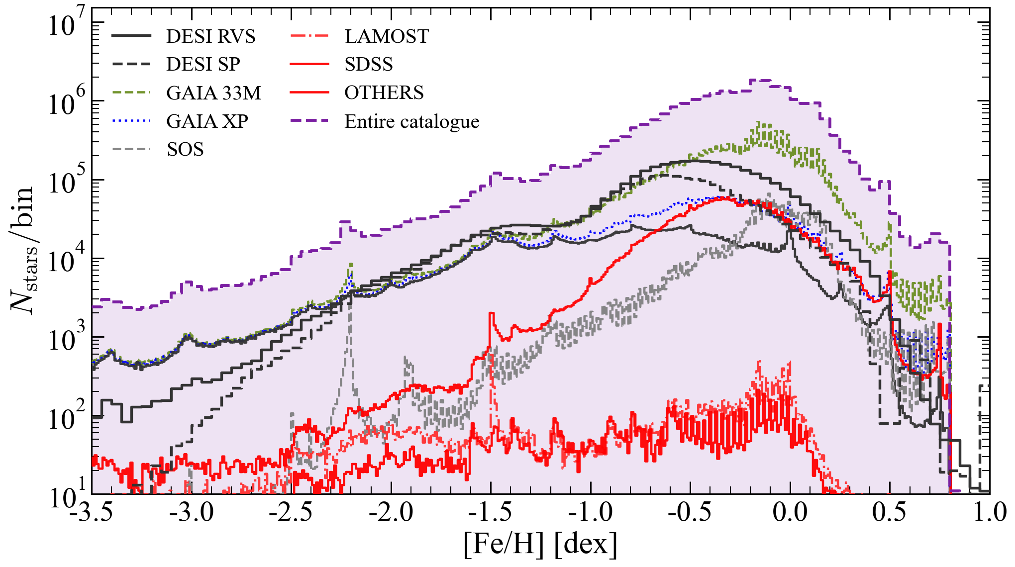
Class

Relation

Reference

Classical Cepheids

M_{V}=-2.76\log_{10}P-1.40

M_{I}=-2.96\log_{10}P-1.81

Madore and Freedman (1991)

Type II Cepheids

M_{K_{s}}=-2.41\log_{10}P-1.02

Matsunaga et al. (2006)

RR Lyrae

M_{K_{s}}=-2.53\log_{10}P+0.07\,[\mathrm{Fe/H}]-0.95

M_{G}=0.32\,[\mathrm{Fe/H}]+1.11

Muraveva et al. (2015); Muraveva et al. (2018)

Miras

M_{K}=-3.51(\log_{10}P-2.38)-7.15

(LMC)

M_{K}=-3.50(\log_{10}P-2.38)-7.25

(Galactic)

Whitelock et al. (2008)

\delta

Scuti

M_{V}=-3.725\log_{10}P-1.969

McNamara (2011)

SX Phe

M_{V}=-3.389\log_{10}P-1.640

McNamara (1997)

Overtone correction

\log_{10}P_{F}=\log_{10}P+0.128

Braga et al. (2015)

Table 10: Comparison of the iterative-clipped raw-row weighted 1D polynomial fits (Ind.) and survey-wise weighted additive multivariate polynomial fits using the same per-parameter orders (Multi.).

Param	$c_{k}$	APOGEE		DESI		GALAH		GES		LAMOST		RAVE		SDSS		Global
		Ind.	Multi.	Ind.	Multi.	Ind.	Multi.	Ind.	Multi.	Ind.	Multi.	Ind.	Multi.	Ind.	Multi.	Ind.
FeH (2)	$N$	194 741	201 726	3 356 610	193 183	113 307	118 550	1 830	2 043	1 210 148	1 167 827	94 085	68 092	13 299	1 835	4 984 020
	$\chi^{2}_{\rm red}$	0.974	–	0.488	–	0.993	–	0.929	–	1	–	0.863	–	0.675	–	0.65
	$c2$	0.17	0.099	-0.068	$5.163\!\times\!10^{-3}$	-0.055	-0.028	0.187	0.407	0.012	-0.151	0.023	-0.432	0.056	0.615	$1.027\!\times\!10^{-14}$
	$c1$	0.248	0.207	0.34	0.106	-0.112	$-4.091\!\times\!10^{-3}$	1.821	0.67	-0.101	-0.266	0.175	-0.047	0.486	1.087	$-4.283\!\times\!10^{-14}$
	$c0$	-0.33	–	-0.238	–	-0.405	–	-0.61	–	-0.161	–	0.603	–	-0.411	–	$-3.982\!\times\!10^{-14}$
Gmag (3)	$N$	280 434	201 726	3 896 979	193 183	150 696	118 550	2 399	2 043	1 441 145	1 167 827	142 381	68 092	18 453	1 835	5 932 487
	$\chi^{2}_{\rm red}$	0.993	–	0.273	–	0.985	–	0.961	–	0.999	–	0.828	–	0.698	–	0.516
	$c3$	$3.506\!\times\!10^{-3}$	$5.031\!\times\!10^{-3}$	$3.226\!\times\!10^{-4}$	$-2.362\!\times\!10^{-3}$	$-2.971\!\times\!10^{-3}$	$-8.618\!\times\!10^{-3}$	-0.048	0.041	-0.013	0.054	0.041	0.154	0.03	0.075	$2.454\!\times\!10^{-11}$
	$c2$	-0.113	-0.151	-0.027	0.079	0.098	0.301	1.659	-1.425	0.563	-1.898	-1.3	-5.001	-1.403	-3.232	$-1.024\!\times\!10^{-9}$
	$c1$	1.21	1.532	0.38	-0.964	-1.026	-3.461	-18.743	15.681	-7.863	21.953	13.512	54.185	21.119	46.062	$1.395\!\times\!10^{-8}$
	$c0$	-4.534	–	-1.123	–	2.907	–	69.007	–	34.627	–	-45.344	–	$-1.036\!\times\!10^{2}$	–	$-6.212\!\times\!10^{-8}$
RV (3)	$N$	303 656	201 726	3 897 147	193 183	160 124	118 550	2 536	2 043	1 510 407	1 167 827	103 563	68 092	18 453	1 835	5 995 886
	$\chi^{2}_{\rm red}$	0.951	–	0.607	–	0.977	–	0.913	–	0.998	–	0.907	–	0.724	–	0.739
	$c3$	$-9.869\!\times\!10^{-8}$	$-1.373\!\times\!10^{-7}$	$-1.693\!\times\!10^{-10}$	$7.621\!\times\!10^{-10}$	$1.192\!\times\!10^{-8}$	$1.847\!\times\!10^{-8}$	$9.369\!\times\!10^{-8}$	$3.583\!\times\!10^{-8}$	$2.211\!\times\!10^{-7}$	$2.523\!\times\!10^{-7}$	$-6.49\!\times\!10^{-7}$	$-4.227\!\times\!10^{-7}$	$3.2\!\times\!10^{-9}$	$-6.396\!\times\!10^{-10}$	0
	$c2$	$3.446\!\times\!10^{-7}$	$2.595\!\times\!10^{-6}$	$-5.423\!\times\!10^{-6}$	$1.87\!\times\!10^{-8}$	$3.092\!\times\!10^{-6}$	$1.438\!\times\!10^{-6}$	$-6.857\!\times\!10^{-6}$	$-3.894\!\times\!10^{-6}$	$6.414\!\times\!10^{-6}$	$1.402\!\times\!10^{-5}$	$2.209\!\times\!10^{-5}$	$-2.814\!\times\!10^{-5}$	$7.478\!\times\!10^{-8}$	$-1.339\!\times\!10^{-7}$	0
	$c1$	$-5.281\!\times\!10^{-4}$	$-3.081\!\times\!10^{-4}$	$3.076\!\times\!10^{-5}$	$-9.291\!\times\!10^{-5}$	$-6.608\!\times\!10^{-4}$	$-9.9\!\times\!10^{-4}$	$-5.67\!\times\!10^{-3}$	$-9.927\!\times\!10^{-4}$	-0.021	-0.022	0.088	0.08	$-1.379\!\times\!10^{-3}$	$-3.278\!\times\!10^{-4}$	0
	$c0$	-0.146	–	-0.315	–	-0.269	–	-0.767	–	-0.291	–	0.276	–	-0.756	–	$-4.056\!\times\!10^{-14}$
SNR (3)	$N$	302 039	201 726	226 831	193 183	160 125	118 550	2 614	2 043	1 383 252	1 167 827	150 255	68 092	2 785	1 835	2 227 901
	$\chi^{2}_{\rm red}$	0.928	–	0.997	–	0.978	–	0.983	–	0.999	–	0.855	–	0.904	–	0.978
	$c3$	$6.252\!\times\!10^{-8}$	$1.092\!\times\!10^{-7}$	$2.921\!\times\!10^{-6}$	$6.152\!\times\!10^{-7}$	$3.232\!\times\!10^{-8}$	$7.062\!\times\!10^{-8}$	$1.828\!\times\!10^{-7}$	$1.637\!\times\!10^{-6}$	$-2.544\!\times\!10^{-7}$	$1.491\!\times\!10^{-7}$	$1.805\!\times\!10^{-8}$	$2.047\!\times\!10^{-9}$	$-8.125\!\times\!10^{-5}$	$-1.032\!\times\!10^{-4}$	0
	$c2$	$-6.177\!\times\!10^{-5}$	$-1.112\!\times\!10^{-4}$	$-5.18\!\times\!10^{-4}$	$-7.667\!\times\!10^{-5}$	$-2.357\!\times\!10^{-5}$	$-4.569\!\times\!10^{-5}$	$-8.695\!\times\!10^{-5}$	$-3.572\!\times\!10^{-4}$	$1.185\!\times\!10^{-4}$	$-6.23\!\times\!10^{-5}$	$-3.329\!\times\!10^{-5}$	$3.735\!\times\!10^{-6}$	$6.396\!\times\!10^{-3}$	0.011	0
	$c1$	0.013	0.022	0.029	$5.189\!\times\!10^{-3}$	$4.977\!\times\!10^{-3}$	$7.924\!\times\!10^{-3}$	$8.206\!\times\!10^{-3}$	$2.092\!\times\!10^{-4}$	-0.011	0.012	0.016	$7.278\!\times\!10^{-3}$	-0.131	-0.249	0
	$c0$	-0.627	–	-0.395	–	-0.439	–	-0.594	–	-0.032	–	-0.146	–	0.535	–	$-4.156\!\times\!10^{-14}$
Teff (3)	$N$	193 380	201 726	3 356 610	193 183	113 099	118 550	1 816	2 043	1 210 548	1 167 827	94 714	68 092	13 299	1 835	4 983 466
	$\chi^{2}_{\rm red}$	0.965	–	0.45	–	0.988	–	0.868	–	1	–	0.871	–	0.667	–	0.625
	$c3$	$-3.793\!\times\!10^{-13}$	$-2.08\!\times\!10^{-14}$	$3.606\!\times\!10^{-12}$	$3.638\!\times\!10^{-14}$	$-7.681\!\times\!10^{-11}$	$-3.918\!\times\!10^{-12}$	$-1.754\!\times\!10^{-12}$	$3.033\!\times\!10^{-11}$	$5.648\!\times\!10^{-12}$	$1.142\!\times\!10^{-12}$	$-3.308\!\times\!10^{-13}$	$1.983\!\times\!10^{-12}$	$1.862\!\times\!10^{-12}$	$4.326\!\times\!10^{-12}$	0
	$c2$	$2.49\!\times\!10^{-8}$	$8.193\!\times\!10^{-8}$	$-7.448\!\times\!10^{-8}$	$7.672\!\times\!10^{-8}$	$1.152\!\times\!10^{-6}$	$-5.025\!\times\!10^{-9}$	$1.098\!\times\!10^{-7}$	$-7.616\!\times\!10^{-7}$	$-1.449\!\times\!10^{-7}$	$2.491\!\times\!10^{-8}$	$2.118\!\times\!10^{-8}$	$-2.757\!\times\!10^{-8}$	$-2.258\!\times\!10^{-9}$	$-4.687\!\times\!10^{-8}$	0
	$c1$	$-4.54\!\times\!10^{-4}$	$-9.132\!\times\!10^{-4}$	$7.045\!\times\!10^{-4}$	$-7.787\!\times\!10^{-4}$	$-5.689\!\times\!10^{-3}$	$4.652\!\times\!10^{-4}$	$-1.711\!\times\!10^{-3}$	$5.717\!\times\!10^{-3}$	$8.17\!\times\!10^{-4}$	$-4.274\!\times\!10^{-4}$	$-3.812\!\times\!10^{-4}$	$6.606\!\times\!10^{-4}$	$8.219\!\times\!10^{-6}$	$1.79\!\times\!10^{-4}$	$-1.031\!\times\!10^{-13}$
	$c0$	1.358	–	-2.511	–	8.873	–	5.237	–	-1.188	–	2.011	–	-1.014	–	$2.448\!\times\!10^{-10}$
logg (2)	$N$	212 563	201 726	3 356 610	193 183	120 380	118 550	1 911	2 043	1 272 904	1 167 827	98 350	68 092	13 299	1 835	5 076 017
	$\chi^{2}_{\rm red}$	0.93	–	0.476	–	0.981	–	0.863	–	1	–	0.875	–	0.664	–	0.647
	$c2$	-0.042	-0.031	-0.26	$-2.546\!\times\!10^{-3}$	0.035	0.062	-0.422	$4.3\!\times\!10^{-3}$	0.112	0.024	0.082	0.068	-0.171	0.239	$2.486\!\times\!10^{-11}$
	$c1$	0.16	0.173	1.618	0.023	-0.235	-0.412	1.943	-0.337	-0.65	-0.013	-0.696	-0.704	0.624	-1.76	$-1.74\!\times\!10^{-10}$
	$c0$	-0.235	–	-2.482	–	0.089	–	-2.467	–	0.608	–	2.052	–	-0.645	–	$2.823\!\times\!10^{-10}$
Shared $\chi^{2}$	$\chi^{2}_{\rm red}$	–	0.87	–	0.995	–	0.935	–	0.948	–	0.997	–	0.905	–	0.875	–
Shared Int.	$b_{0}$	–	-4.031	–	6.22	–	11.551	–	-66.508	–	-83.966	–	$-1.975\!\times\!10^{2}$	–	$-2.142\!\times\!10^{2}$	–

Figure 28: Absolute radial-velocity uncertainty (

\sigma_{v_{r}}

) as a function of heliocentric distance (

d_{\rm helio}

). The solid blue curve illustrates the median uncertainty for the final merged catalogue, while the solid orange curve represents the estimates from the GAIA DR3 33M RVS sample. The shaded regions and dashed lines correspond to the

16^{\rm th}

–

84^{\rm th}

percentile bands for each respective dataset