Optical and Dynamical Signatures of Padé Approximated Wormholes in Gravity
Abstract
We construct traversable wormhole solutions in the linear teleparallel model , adopting Padé approximants of order [1/0] and [0/1] as shape functions together with the redshift function , and derive the corresponding source terms from the modified field equations. We assess the physical viability of both configurations through the energy conditions, Tolman–Oppenheimer–Volkoff equilibrium, the volume integral quantifier, thin-shell junction matching to an exterior Schwarzschild vacuum, embedding diagrams, proper radial distance, the gravitational energy and the active mass. We then examine the observational signatures of each geometry by analysing equatorial null geodesics and the photon-sphere structure, computing shadow maps and radial intensity profiles, ray-tracing relativistic images of a geometrically thin accretion disc, and integrating timelike rosette orbits. Finally, we study the dynamical stability of both wormholes through a third-order WKB quasinormal-mode analysis across scalar, electromagnetic, and axial gravitational perturbations, cross-checked against time-domain evolution and the eikonal photon-sphere correspondence, and examine the parameter dependence of the mode spectrum together with the possibility of trapped-mode echoes.
I Introduction
The quest to extend Einstein’s general theory of relativity beyond its classical domain has driven substantial progress in gravitational physics over the past several decades. Among the most well-studied extensions is teleparallel gravity and its generalizations, wherein the gravitational field is described not through spacetime curvature but through torsion arising from the Weitzenböck connection [83, 110, 30, 22]. The gravity framework, which replaces the torsion scalar in the teleparallel equivalent of general relativity with an arbitrary function , has attracted considerable attention as a geometrically distinct, yet physically rich alternative to both general relativity and curvature-based modified theories such as gravity [18, 11, 56]. The modified field equations in gravity yield richer phenomenology in strong-field regimes, including corrections to black hole thermodynamics, modified gravitational wave propagation, and new classes of compact object solutions. These features make gravity a compelling arena for investigating exotic spacetime geometries, particularly traversable wormholes, whose construction in general relativity typically requires violations of the null energy condition attributed to exotic matter. However, in gravity, such configurations can be supported more naturally by torsion-induced geometric corrections [79, 80, 107, 113, 94].
Traversable wormholes, first placed on rigorous footing by Morris and Thorne [71], represent topological bridges connecting distinct regions of spacetime and have evolved from purely theoretical constructs [44, 38] into objects of active observational interest. In modified gravity frameworks, including , , and teleparallel formulations, the effective stress-energy contributions arising from geometric modifications can partially or fully replace the exotic matter otherwise required to sustain the wormhole throat [93, 72, 90, 95, 46, 96, 47, 124, 39, 105, 5, 70, 2, 78, 122]. The astrophysical significance of traversable wormholes has grown in parallel with the maturation of gravitational-wave astronomy and high-resolution very-long-baseline interferometry, both of which open windows onto compact object signatures that may distinguish wormholes from black holes [33, 58, 106, 52, 85]. In particular, the formation of photon spheres, the divergence of the deflection angle in the strong-field limit, and the structure of shadow images cast by compact objects under strong gravitational lensing provide powerful observational probes of the underlying spacetime geometry [97, 45, 120, 15, 17, 12, 16, 119]. Gravitational lensing in wormhole spacetimes has been extensively studied, including deflection angle calculations [77, 89, 37, 13, 1, 73, 104, 116, 115, 74, 75], analyses of negative-mass wormholes [31, 92], convergent lens behavior [114], and the characterization of photon and antiphoton sphere structures [101, 19, 99, 35, 36, 4, 60, 100]. The Event Horizon Telescope’s imaging of compact object shadows has further sharpened the need for detailed theoretical predictions of shadow morphology in alternative spacetime backgrounds, including those generated by wormhole geometries in modified gravity [61].
A central technical challenge in modeling wormhole observables is the construction of physically admissible shape functions that simultaneously satisfy throat regularity, the flare-out condition, and asymptotic flatness across the full radial domain [121, 70, 2, 78]. Shape functions derived from truncated Taylor series often fail to reproduce physically consistent behavior at large radial distances or in the strong-field region near the throat. Padé approximants, rational functions constructed as ratios of polynomials matched to a given power series [6], provide a systematic and analytically tractable improvement over Taylor truncations by encoding pole structure and extending the convergence domain [23, 51]. Their application to wormhole modeling has been demonstrated to transform inadequate or analytically intractable shape functions into viable candidates that satisfy all required geometric constraints, while remaining amenable to closed-form analysis and numerical integration of geodesic equations [24, 112, 27]. The stability and convergence behavior of Padé approximants, including the role of spurious poles and the limitations of higher-order approximations, have been analyzed in the mathematical literature and carry direct implications for their use in wormhole modeling [109, 9, 111]. The utility of Padé approximants in cosmography [23, 51] and in and wormhole frameworks [24, 112] further motivates their systematic deployment in torsion-based gravitational theories.
Previous investigations have examined wormhole solutions in various modified gravity settings and have separately studied Padé approximants as tools for shape function construction or cosmographic modeling. Shadow formation and photon sphere structure in wormhole spacetimes have been studied within general relativity and selected curvature-based modified gravity frameworks [101, 52, 36, 19]. Padé-based shape functions have been applied in and gravity to improve analytical control of wormhole geometries [24, 112]. Charged wormhole geometries with photon sphere analysis and energy condition investigations have been conducted within the framework [46, 96], and wormhole solutions in teleparallel-inspired models have been reported in the literature [80, 94]. Nevertheless, no prior study has integrated the gravity framework with Padé-approximated metric functions to perform a combined analysis that encompasses null geodesic structure, determination of the photon sphere by ray tracing, shadow imaging, and emission of accretion disks with intensity mapping. This gap in the literature leaves the observational signatures of wormholes quantitatively unexplored and the utility of Padé approximation within torsion-based gravity unaddressed.
The present work addresses these open questions by constructing traversable wormhole solutions within gravity and applying Padé approximants to the relevant metric functions to obtain physically consistent and analytically tractable forms. The null geodesic equations are derived and analyzed to determine the structure of the photon sphere, with the effective potential examined as a function of the Padé approximant parameters and the coupling. Ray tracing techniques are employed to map null trajectories in the wormhole spacetime and compute the resulting shadow images, and the bound photon trajectories are further investigated through the rosette orbit structure. The study further incorporates a relativistic accretion disk model around the wormhole throat, from which specific intensity maps are produced to characterize the luminosity profile as seen by a distant observer. We additionally examine the dynamical stability of the constructed wormhole configurations through a quasinormal mode (QNM) analysis, computing the characteristic ringdown frequencies under scalar perturbations using the WKB approximation [98, 57, 65] and studying their dependence on the Padé parameters and the coupling. Quasinormal modes encode the response of the wormhole to external perturbations and serve as a robust probe of dynamical stability and a potential observational discriminator between wormholes and black holes [63, 10, 64, 25, 29, 20]. Together, these analyses provide a comprehensive theoretical framework for the observational phenomenology of wormholes and establish Padé approximation as a practical and powerful tool within torsion-based modified gravity.
The outline of the present paper is as follows: Sec. II sets up the wormhole construction in teleparallel gravity, and Sec. III derives the and Padé shape functions and their source terms. Sec. IV assesses the physical viability of both configurations, while Sec. V examines their observational signatures. The quasinormal modes and linear stability are studied in Sec. VI, and we conclude in Sec. VII.
II Wormhole Construction in Teleparallel Gravity
In teleparallel gravity the dynamical variable is the tetrad field , related to the metric by , with , inverse obeying , and . Capital Latin indices label the tangent frame, Greek indices the spacetime coordinates. The curvature-free Weitzenböck connection () defines the torsion tensor,
| (1) |
from which the torsion scalar is constructed as
| (2) |
where and is the contorsion tensor given by
| (3) |
The Einstein-Hilbert action for gravity is
| (4) |
where . The variation with respect to the tetrad yields the field equations [3]
| (5) |
where , , and is the matter energy-momentum tensor, can be expressed as
| (6) |
The static, spherically symmetric Morris–Thorne metric is [71]
| (7) |
where is the redshift function and is the shape function. The radial coordinate satisfies , with the throat radius. For a traversable wormhole, must satisfy:
- •
(throat condition),
- •
(flare-out condition),
- •
(derivative bound at throat),
- •
for all ,
- •
as (asymptotic flatness).
In addition, must remain finite for all to prevent event horizon formation.
The diagonal tetrad compatible with Eq. (7) is
| (8) |
for the above choice of tetrad, the non-vanishing torsion components (1) are
| (9) |
where, . Therefore, inserting Eq. (8) into Eq. (1)–(2) gives
| (10) |
In this work, we adopt the linear model,
| (11) |
where and are the model parameters. With the derivative-coupling term in (5) vanishes and, for the diagonal tetrad (8), the off-diagonal field equation is satisfied identically. The diagonal components reduce to the effective relations
| (12) |
where is the anisotropic source and is the mixed Einstein tensor of the Levi-Civita connection. The sign of the geometric term follows the teleparallel convention fixed by (10). The nonzero components of are
| (13) | ||||
| (14) | ||||
| (15) |
Substituting (13)–(15) into (12) yields the field equation for gravity,
| (16) | ||||
| (17) | ||||
| (18) |
The explicit forms follow once is fixed in (Sec. III). Throughout this study, we adopt the asymptotically flat redshift function , a horizon-free inverse- ansatz that has been employed in wormhole studies of photon trajectories, photon spheres, and shadow observables [118, 40]. This choice ensures that remains finite throughout the spacetime and vanishes asymptotically as , thereby preserving traversability and asymptotic flatness. For this form, and , both of which decay at large distances.
III Padé Approximation and Source
The Padé approximation is a technique for representing a function as the ratio of two polynomials. For a function whose Taylor (Maclaurin) series expansion about is known, the corresponding Padé approximant reproduces that series up to the highest possible order while expressing the function in rational form. A Padé approximant of order is written as [6]
| (19) |
where and are the degrees of the numerator and denominator polynomials, respectively, and the coefficients and are real constants. Without loss of generality, one conventionally normalizes the leading denominator coefficient as , which fixes the overall scale of the rational function and leaves independent coefficients to be determined.
These coefficients are obtained by demanding that the Taylor expansion of agree with the Taylor series of the function to as many orders as possible, i.e.
| (20) |
so that the first terms of the two expansions coincide.
In the present work, we employ the Padé approximation to model the shape function of the wormhole geometry. By expressing in rational form, we obtain a flexible yet analytically tractable ansatz whose free coefficients can be fixed by imposing the standard physical requirements on the shape function—namely the throat condition, the flaring-out condition, and asymptotic flatness. In this paper, we specifically consider the two lowest-order approximants, the and orders, which represent the simplest non-trivial rational forms of and are analyzed in detail in the following subsections.
III.1 The -Order Padé Approximant
For the order, the numerator is linear and the denominator reduces to a constant (with ), so that Eq. (19) takes the simple polynomial form
| (21) |
This represents the lowest-order non-trivial approximant, i.e. a linear function of the radial coordinate.
To construct the shape function in this order, we begin from the seed function [49]
| (22) |
where is a free parameter and we have defined,
| (23) |
Since the approximant is linear in , we expand the seed function to the first order about the throat . The Taylor expansion of around reads
| (24) |
Next, we expand the power about , retaining only the linear term consistent with the order,
| (25) |
Truncating Eq. (24) at first order gives , so that
| (26) |
Substituting Eq. (26) into the seed function (22) produces the shape function at the order,
| (27) | |||
| (28) |
By construction this form satisfies the throat condition , as is evident by setting in Eq. (28).
We now verify the geometric requirements with the parameters , , , and . The flaring-out condition, expressed through the combination , ensures that the wormhole opens outward in the vicinity of the throat. As shown in Fig. 1, this quantity remains strictly positive over the entire radial domain, decreasing monotonically from its maximal value at the throat and tending to zero at large , so that the flaring-out condition is satisfied. At the throat itself the derivative of the shape function obeys the bound ; for the present case we find , which lies safely below unity and is consistent with the throat being a minimum of the embedded geometry.
The final constraint, as , warrants more careful analysis. As shown in Fig. 2, the ratio starts from unity at the throat and decreases monotonically thereafter, staying strictly below for all . However, since the shape function grows linearly in , the ratio does not vanish but instead approaches a small but finite constant at large , so that strict asymptotic flatness is not recovered. This residual value does not signal a pathology: the linear growth of endows the geometry with a solid-angle deficit at large scales, indicating that the wormhole behaves as a topological defect of the global-monopole type rather than as an exactly asymptotically flat spacetime. The constraint can therefore be relaxed in the same spirit, with asymptotic flatness holding only approximately while the global structure remains physically admissible.


For this above and the redshift function mentioned in section-II, the field Eqs. (16-18) reduces to,
| (29) | |||||
| (30) | |||||
| (31) |
Where,
III.2 The -Order Padé Approximant
For the order, the situation is reversed with respect to the previous case: the numerator reduces to a constant while the denominator is linear in the radial coordinate. After normalizing the leading denominator coefficient, Eq. (19) takes the rational form
| (32) |
where collects the single independent coefficient that survives after normalization.
We proceed from the same seed function and Taylor expansion employed in the previous subsection. Truncating Eq. (24) at first order about the throat gives
| (33) |
In contrast to the case, where the power was represented as a linear polynomial, here we recast it in rational form so as to match the structure of Eq. (32). To this end we write
| (34) |
The equivalence of this representation with the linear one, to the order considered, follows from the geometric-series expansion
| (35) |
so that, identifying ,
| (36) |
Both the and approximants thus share the same first-order Taylor expansion, as required, but differ in their behavior away from the throat.
Substituting Eq. (34) into the seed function (22), , gives the closed form of order shape function as,
| (37) |
We now examine the same geometric conditions with the parameters , , , and . The flaring-out quantity is shown in Fig. 3, where it remains strictly positive across the radial domain and grows steadily with , confirming that the flaring-out condition holds for this approximant. The derivative of the shape function at the throat satisfies the bound ; here we obtain , which is negative and therefore comfortably below unity, reflecting the monotonic decay of the shape function away from the throat. Lastly, the ratio is plotted in Fig. 4, where it begins at unity at the throat and decreases monotonically, remaining strictly below for all and approaching zero at large .


IV Physical Analysis
IV.1 Energy Condition
The classical point wise energy conditions for such a anisotropic matter source are expressed through the combinations [121, 68]
| NEC: | (41) | |||
| WEC: | (42) | |||
| SEC: | (43) | |||
| DEC: | (44) |
The null energy condition (41) is the weakest of the four and controls the existence of the throat. For an anisotropic source the NEC splits into two independent channels, the radial combination and the tangential combination , and the NEC is violated whenever either channel turns negative [108, 55, 68]. For the Morris–Thorne geometry the flaring-out condition of Sec. II forces at least one of these null combinations negative in a neighbourhood of , so a violation of the NEC at the throat is the defining signature of the exotic matter required for traversability. The energy conditions corresponding to the and order approximants are illustrated in Fig. 5 and Fig. 6, respectively.

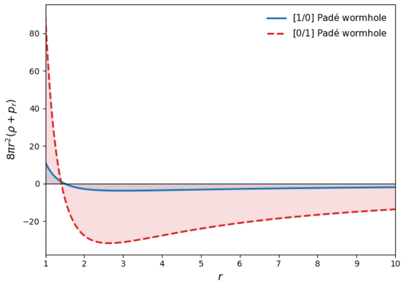
From Fig. 5, the energy density at the throat is negative, , and the tangential null combination is also negative, , while the radial null combination is positive, . Since one of the two null channels is negative, the NEC (41) is violated at the throat through the tangential channel, which suffices to identify the matter as exotic. The energy density increases monotonically away from the throat, changes sign in the near-throat region, and approaches its asymptotic value as . The tangential combination remains negative across the entire exterior and approaches zero from below, so the tangential NEC stays violated everywhere and is only marginally restored at spatial infinity, whereas the radial combination stays positive throughout. With at the throat the WEC (42) fails as well, and the negative values and show that the DEC (44) also fails. The strong-energy combination at the throat and remains negative for all , so the SEC (43) is violated throughout.

For the order approximant, the energy density at the throat is large and positive, , the radial null combination is positive, , while the tangential null combination is negative, . The negative tangential channel again drives a violation of the NEC (41) at the throat. Although here, the negative means the WEC (42) still fails through its tangential condition, and the values and show that the DEC (44) fails in the tangential channel. The strong-energy combination is strongly negative at the throat, , and remains negative across the exterior, so the SEC (43) is violated as well.
In both Padé orders the tangential null combination is negative at the throat, so the NEC is violated there and the matter source is exotic, in agreement with the flaring-out requirement of Sec. II. In both cases the WEC, SEC, and DEC are also violated, which establishes that the linear model with the Padé shape functions supports a traversable wormhole sustained by NEC-violating matter. The radial null combination remains positive in both branches, so the violation is carried entirely by the tangential channel, a feature shared with other anisotropic wormhole constructions in modified gravity [68].
IV.2 Tolman–Oppenheimer–Volkoff Equilibrium
The Tolman–Oppenheimer–Volkoff (TOV) equation [86] governs the gravitational equilibrium of a static, spherically symmetric matter distribution and provides a standard diagnostic of the stability of wormhole solutions [48]. For an anisotropic source, the generalized TOV equation reads [66]
| (45) |
where is fixed by the redshift function. The three terms represent the gravitational, hydrostatic, and anisotropic forces,
| (46) |
and equilibrium requires their sum to vanish,
| (47) |
Unlike wormhole studies adopting a constant redshift function, where removes entirely, the present work employs the asymptotically flat redshift of Sec. II, for which . The gravitational force is therefore active throughout, and all three contributions in Eq. (47) must be retained.
For the linear model adopted here, and the theory is dynamically equivalent to the teleparallel equivalent of general relativity supplemented by a constant. The effective source is then identically conserved , by virtue of the contracted Bianchi identity, so no additional modified-gravity force arises and the standard anisotropic balance (47) holds exactly. Moreover, the constant enters , , and only as an additive shift that cancels in every combination in Eq. (46); the equilibrium forces are thus independent of and are controlled by , , , and the Padé parameter alone.
The behaviour of the three forces is shown in Fig. 7 and Fig. 8 for the and orders, with , , , , and the Padé parameter fixed at and respectively. In both cases the hydrostatic force is positive and directed outward, while the gravitational and anisotropic forces and are negative and directed inward; their sum vanishes identically throughout the spacetime, confirming that condition (47) is satisfied. The forces are largest near the throat and decay rapidly at large , where the geometry approaches flat space. The two Padé orders produce qualitatively identical equilibrium structures, differing only quantitatively in the near-throat region: the branch develops substantially larger force magnitudes at the throat than the branch, consistent with its steeper shape function. This exact cancellation demonstrates that the wormhole configurations obtained in both Padé orders are in stable hydrostatic equilibrium under the combined action of the hydrostatic, gravitational, and anisotropic forces.


IV.3 Volume Integral Quantifier
The Volume Integral Quantifier (VIQ) serves as a crucial tool to measure the total exotic matter required to maintain a traversable wormhole. For spherically symmetric wormholes, it is defined as
| (48) |
where is the energy density, the radial pressure, the throat radius, and a finite cutoff radius introduced to regularize the integral. This quantity effectively captures the average violation of the NEC necessary for wormhole stability [7]. While powerful, the VIQ may diverge unless properly regularized, typically through junction conditions that impose a cutoff radius; notably, wormholes with conformal symmetry or supported by phantom energy can achieve arbitrarily small VIQ values, potentially connecting wormhole physics to cosmic acceleration scenarios [68].
We fix the throat radius at and plot the integrand as a function of for both wormhole solutions in Fig. 9.
The integration domain runs from the throat to the cutoff radius , chosen according to the junction-condition formalism, where the interior geometry is matched to an exterior Schwarzschild vacuum at the boundary where the influence of the exotic core has become negligible [113]. For both solutions, the integrand approaches a slowly varying, non-divergent profile well before , so that encloses the region in which the dominant NEC-violating contribution is generated. The numerical integration of Eq. (48) yields
| (49) |
Both results are finite and negative, confirming that NEC-violating (exotic) matter is required to support each geometry within the linear model. As seen in Fig. 9, both integrands are positive in a narrow region just outside the throat () before turning negative; the integrand then saturates at a small, slowly decaying negative tail, so that is dominated by this broad, shallow negative contribution. By contrast, the integrand develops a deep negative minimum just outside the throat () before relaxing slowly toward zero; the much larger magnitude reflects this pronounced near-throat concentration of exotic matter, consistent with the steeper fall-off of the shape function. In both cases the finiteness of over the matched interior region demonstrates that a bounded amount of NEC-violating matter suffices to sustain the wormhole throat for the chosen parameters.
IV.4 Embedding Surface and Diagrams
Following Morris and Thorne [71], the spatial geometry of the wormhole is visualized by embedding the equatorial slice , of the metric (7) into a three-dimensional Euclidean space with cylindrical coordinates , whose line element is . Matching this to the induced two-geometry of the slice yields the embedding function , satisfying
| (50) |
whose slope diverges at the throat, as , so that the embedded surface is vertical there—the defining geometric signature of a wormhole throat. Integrating outward from the throat,
| (51) |
gives the two symmetric sheets and that join smoothly at and connect the two asymptotically flat regions. The integral for both Padé order and is evaluated numerically.
The resulting profiles for the and shape functions, computed for several throat radii with and , are shown in Fig. 10 (with both the and sheets plotted) and tabulated in Table 1. Each profile is vertical at its own throat and flares outward monotonically, in agreement with the flaring-out condition imposed in Sec. III. The full embedded surfaces, obtained by revolving these profiles about the -axis through , are displayed in Fig. 11. They exhibit the characteristic wormhole morphology: a narrow circular throat of radius that widens smoothly into two flared mouths. Both Padé orders produce qualitatively the same throat geometry, differing in the rate of flaring away from the throat: the linear shape function yields a more steeply rising profile reaching at , whereas the pole-free shape function flares more gradually, reaching only over the same range, consistent with the slower growth of its shape function.


IV.5 Proper Radial Distance
The proper radial distance measures the physical distance from the throat to a point as measured by a static observer, and must remain finite and positive everywhere outside the throat for the wormhole to be traversable. It is given by
| (52) |
with the plus (minus) sign corresponding to the upper (lower) universe connected by the wormhole. As with , the integral cannot be solved analytically for the Padé shape functions of Sec. III and is evaluated numerically. Since holds throughout for and , the integrand remains real and finite for all , with an integrable inverse square-root singularity at the throat itself. The resulting profiles of are shown in Fig. 12 and tabulated alongside and in Table 1. The profiles rise more steeply than the profiles at fixed , reaching against near for , reflecting the slower growth of the pole-free shape function.

IV.6 Gravitational Energy and Active Mass
Two integral diagnostics built from the energy density characterize the mass-energy content of the wormhole. The first is the total gravitational energy , defined via the Lynden-Bell–Katz–Nandi prescription [82, 62, 76] as the difference between the total energy and the total mechanical energy , , which reduces to
| (53) |
The second is the active gravitational mass enclosed between the throat and a radius [67, 27],
| (54) |
While Eq. (53) is evaluated numerically owing to the complexity of the integrand, the active mass admits a closed form. For the linear model , so that
| (55) |
using the throat condition . This yields , so the active mass vanishes at the throat, and , so increases where and decreases where .
The profiles of and are shown in Fig. 13 and Fig. 14 respectively, for several throat radii , and the numerical values of , , and are collected in Table 1 for three representative radii . The two diagnostics behave very differently between the branches. For the order the gravitational energy starts positive at the throat, , rises to a maximum in the near-throat region, and then decreases, turning negative at larger as the negative-energy-density region begins to dominate the integral; the active mass likewise dips negative just outside the throat before recovering and increasing. For the order the gravitational energy decreases monotonically from and is negative across most of the displayed range, whereas the active mass is large and positive and grows steeply with , since the energy density for this branch is positive and rises rapidly away from the throat. We emphasize that these sign changes are not pathological but are the expected quasilocal-energy signature of the null-energy-condition-violating matter established in Sec. IV: a region of negative energy density generically drives the gravitational energy and active mass negative in its vicinity, a feature documented for exotic wormhole sources in general relativity [67, 76] and in modified gravity [27]. The contrasting behaviour of the branch, where even though , arises from the geometric weighting factor in Eq. (53), which renders the gravitational energy negative for a positive energy density and is therefore a property of the strong-field geometry rather than of the sign of the source. The sign and slope of both quantities are thus controlled by the sign of together with the geometric factor in each branch, in accordance with . This behaviour is consistent with the energy-condition analysis of Sec. IV, where the branch has negative throat energy density and the branch positive, and it confirms a physically sensible distribution of gravitating mass-energy in both Padé orders.


| 1.41 | 0.584207 | 0.584662 | 0.353857 | 0.257554 | 0.258587 | |
| 1.43 | 0.827519 | 0.828803 | 0.204034 | 0.363888 | 0.366803 | |
| 1.45 | 1.015119 | 1.017469 | 0.081529 | 0.445245 | 0.450590 | |
| 1.49 | 1.314675 | 1.319697 | 0.573719 | 0.585177 | ||
| 1.51 | 1.442425 | 1.449004 | 0.627885 | 0.642920 | ||
| 1.30 | 0.927419 | 0.929206 | 0.457521 | 0.381691 | 0.386023 | |
| 1.35 | 1.317641 | 1.322647 | 0.341257 | 0.538331 | 0.550521 | |
| 1.40 | 1.621152 | 1.630261 | 0.218863 | 0.657554 | 0.679834 | |
| 1.45 | 1.880397 | 1.894290 | 0.087068 | 0.757270 | 0.791400 | |
| 1.50 | 2.117723 | 2.130962 | 0.844440 | 0.891903 | ||
| 1.25 | 0.929645 | 0.931428 | 0.564282 | 0.372518 | 0.376954 | |
| 1.30 | 1.321168 | 1.326158 | 0.501252 | 0.525319 | 0.537801 | |
| 1.35 | 1.625926 | 1.635003 | 0.419881 | 0.641573 | 0.664382 | |
| 1.40 | 1.886427 | 1.900265 | 0.323012 | 0.738766 | 0.773699 | |
| 1.45 | 2.119034 | 2.138189 | 0.212068 | 0.823699 | 0.872268 | |
V Observational Analysis
V.1 Null Geodesics and Photon Trajectories
Light propagation is the most direct observational probe of the wormhole geometry, since the location of the photon sphere and the associated critical impact parameter fix the angular size of the shadow and govern strong-field lensing [120, 17, 116, 101]. We analyse equatorial null geodesics of the metric (7) for the two Padé shape functions.
By spherical symmetry, a null geodesic with initial data in the equatorial plane remains in . The Lagrangian is independent of and , so the energy and angular momentum
| (56) |
are conserved, with the overdot denoting . Imposing the null condition and rescaling the affine parameter so that yields
| (57) |
| (58) |
where is the impact parameter. Equation (57) has the form with photon potential , so the radial motion is controlled by the function
| (59) |
through the turning-point condition .
A circular null orbit requires together with its radial derivative, which away from the throat reduces to , i.e. . This condition involves only the redshift function, so the photon-sphere radius is independent of the shape function and of the Padé order. For ,
| (60) |
which has a single extremum, a minimum, at
| (61) |
The minimum of corresponds to an unstable circular photon orbit [116, 74]: rays with reach an outer turning point and are deflected, rays with have no turning point and plunge to the throat, and is the critical curve that bounds the shadow. When the photon sphere lies in the accessible exterior; when the extremum is hidden behind the throat, is monotonic on , and the throat itself acts as the capture boundary with limiting impact parameter . The shape function does not move the photon sphere; it controls the bending away from through the factor in (57), and hence the winding structure and the asymptotic behaviour of the deflected rays.
The two branches are integrated with the coupling parameters fixed at the values that keep each shape function well behaved on . For the form we take , for which stays positive; for the form, we take , which moves the pole below the throat, leaving pole-free and asymptotically flat, with . The redshift mass is fixed in each panel so that the photon sphere lies outside the throat: with for the branch, and for the branch. In every panel , so a photon sphere of radius and a shadow of radius are present; the choice of rescales the figure without altering these qualitative features.
Equations (57)–(58) are integrated with an adaptive Runge–Kutta scheme (relative tolerance ) for six throat radii . Rays are launched from with a range of impact parameters densely sampled around , integration terminating at the radial turning point (deflected rays) or at the throat (captured rays). The deflected branch is completed by the reflection symmetry of the orbit about its turning point. Results are shown in Fig. 15(a) for the branch and Fig. 15(b) for the branch.


Both branches share the same photon-sphere radius and critical impact parameter , because these depend on alone (61). The difference between Figs. 15(a) and 15(b) is therefore entirely due to the shape function entering . In the case the linear shape function approaches a constant fraction , so the exterior carries a residual deficit and even distant rays are curved, giving the broad winding seen in Fig. 15(a); here is a coordinate quantity rather than the true geometric impact parameter at infinity. In the case with the shape function decays as , so , the exterior is asymptotically flat, coincides with the asymptotic impact parameter, and the lensing is confined to a compact region around , as in Fig. 15(b). The asymptotically flat geometry is the most suitable of the two for shadow and lensing observables, while both reproduce the same shadow radius set by the redshift [101, 99, 61].
V.2 Intensity Profiles and Shadow Maps
The optical appearance of a compact object illuminated by an optically thin emission region encodes the geometry of its photon region and serves as a direct observational probe of the underlying spacetime [118, 101]. The Event Horizon Telescope images of M87∗ and Sgr A∗ have established horizon-scale imaging as a quantitative test of gravity theories and exotic alternatives to black holes, including wormholes [118]. Wormhole shadows and their gravitational-lensing signatures have consequently been studied across a wide range of geometries and matter models [102, 81, 101, 99, 8], with strong-deflection lensing providing a complementary diagnostic of the throat region [116, 115, 17, 77].
For the static spherically symmetric metric of Eq. (7) with redshift function , null geodesics are governed by the conserved energy and the angular momentum, whose ratio defines the impact parameter . Photon trajectories follow from the radial equation derived from the null condition, and the effective potential governing the radial motion is set by the combination , whose extremum fixes the photon sphere and the associated critical impact parameter [120, 17]. For the redshift profile adopted here, the critical impact parameter takes the compact form , in agreement with the value obtained for exponential-metric wormholes in the literature [14, 117]. This critical curve separates photons that are captured or transmitted through the throat from those that are deflected back to a distant observer, and its angular size on the observer’s sky determines the boundary of the shadow [102, 101].
We modeled the observed specific intensity by integrating the emissivity of an optically thin accretion flow along each null geodesic, accounting for the gravitational redshift of the radiation through the factor [8, 118]. The radiative-transfer integral assigns to each impact parameter a total intensity built from the redshift-weighted emissivity and the path-length element along the trajectory, with photons possessing a radial turning point that contributes an additional passage through the emitting region. The numerical integration of null geodesics is carried out with an adaptive scheme, terminating each ray either at its radial turning point or upon reaching the throat, which acts as the effective capture surface for the present geometry [102].
We evaluated the intensity for both Padé-approximant wormhole geometries constructed in Sec. III: the -order branch, Eq. (28), and the pole-free -order branch, Eq. (37). For each branch we consider a sequence of throat radii , with for the branch and for the branch. To enable a faithful comparison across throat radii and between the two branches, all intensity profiles are normalized by a single global maximum, and all impact-parameter scans share a common range, so that both the relative brightness and the relative angular size of the features are preserved rather than rescaled panel by panel.
The radial intensity profiles are shown in Fig. 16(a) for the -order wormhole and in Fig. 16(b) for the -order wormhole. In every panel the intensity rises from a finite value near the optical axis, attains a sharp maximum at the critical impact parameter (marked by the dashed line), and decays monotonically toward larger . The peak at is the photon-ring enhancement: rays with close to wind multiple times near the photon sphere and accumulate a large path length through the emitting medium, producing the characteristic bright ring familiar from black-hole and wormhole imaging [101, 8, 118]. As increases, the associated mass and hence shift to larger values, so the peak migrates outward while its normalized height decreases, reflecting the reduced redshift enhancement for the more extended, lower-compactness configurations.
The corresponding two-dimensional shadow maps, rendered as an axially symmetric radial colour gradient with the critical curve overlaid, are displayed in Fig. 17(a) for the -order wormhole and in Fig. 17(b) for the -order wormhole. In each panel the dashed white circle marks the critical curve at the radius , which sets the boundary of the shadow on the observer’s sky. Because all panels are rendered on a common radial scale, the systematic growth of the critical curve with increasing is directly visible: larger throat radii yield larger and therefore larger shadows on the observer’s sky. A comparison of the two branches at fixed reveals that the -order geometry, for which exceeds the value by a factor of a few, produces a substantially larger critical curve, while the pole-free geometry yields a more compact, centrally concentrated critical curve. This contrast underscores the sensitivity of the shadow size to the specific shape-function ansatz, in line with the broader finding that wormhole observables discriminate effectively between competing geometries and gravity models [102, 101, 118].


Taken together, the intensity profiles and shadow maps demonstrate that both Padé-approximant wormholes in the linear model produce the photon-ring and shadow morphology characteristic of horizon-scale compact objects, with the shadow size scaling monotonically with the throat radius and depending sensitively on the shape-function branch [102, 101, 118]. These features place the present geometries within the class of wormhole spacetimes whose optical signatures could, in principle, be confronted with high-resolution very-long-baseline interferometric observations [118, 101].
V.3 Accretion Disc Images
The intensity profiles and shadow maps of Sec. V.2 describe the lensing of an idealized, axisymmetric emission ring. A complementary and more directly observable proxy is the relativistically imaged accretion disc, whose brightness distribution on the sky carries the combined imprint of gravitational lensing, frame-dependent Doppler boosting, and gravitational redshift in the strong-field region [69, 32, 118]. The horizon-scale images of M87∗ and Sgr A∗ recorded by the Event Horizon Telescope have made such disc images a quantitative test of the near-horizon geometry [41, 42, 43], and horizonless compact objects, including wormholes, are now routinely examined as black-hole mimickers whose disc morphology can be confronted with very-long-baseline interferometry [100, 74, 75, 8, 101]. Accretion onto wormhole geometries and the associated optical signatures have been studied for a range of matter models and gravity theories [35, 36, 54].
We construct the images by backward ray tracing. For each pixel of the observer’s image plane, parametrized by the celestial coordinates at inclination , a null geodesic is launched toward the source and integrated with a fixed-step fourth-order Runge–Kutta scheme. The trajectory is governed by the geodesic equations of the metric in Eq. (7) with redshift function and the Padé-approximant shape functions of Sec. III, the -order branch of Eq. (28) and the pole-free -order branch of Eq. (37). The conserved energy and axial angular momentum fix the initial momenta on the image plane, with the radial momentum set by the null condition [17, 120]. Each ray is terminated either upon escaping to large radius or upon reaching the throat at , which acts as the effective capture surface for the present horizonless geometry [102, 116, 115].
The emitting matter is modeled as a geometrically thin optically thin disc lying in the equatorial plane, extending from an inner edge to an outer edge , with a Gaussian vertical profile of half-thickness and a phenomenological radial emissivity with [84, 87, 103]. The disc material follows circular geodesics with orbital angular velocity
| (62) |
and the radiation is transported along the null geodesics with the frequency ratio of observed to emitted photons,
| (63) |
which combines the gravitational redshift with the Doppler shift of the orbiting source [32, 69, 8]. By Liouville’s theorem the observed specific intensity accumulated along each ray scales as
| (64) |
with the height above the equatorial plane, so that the steep dependence produces the strong brightness asymmetry between the approaching and receding sides of the disc characteristic of near-edge-on viewing [69, 59, 118].
Figure 18(a) shows the resulting images for the -order wormhole with , for throat radii . Each panel displays the bright, Doppler-boosted crescent on the approaching side of the disc, a central brightness depression bounded by the photon ring, and a lensed secondary image of the far side of the disc arching above and below the shadow, the hallmark morphology of strongly lensed accretion flows around compact objects [69, 43, 50]. Because the field of view and the observer distance are held fixed in physical units across the sequence, the steady growth of the shadow and photon ring with directly reflects the increase of the associated mass with throat radius [14, 117].


Figure 18(b) shows the corresponding images for the pole-free -order wormhole with . Here, the field of view and the observer distance are scaled in proportion to , so the rendered images are approximately self-similar across and isolate the morphology intrinsic to the shape-function branch. The geometry yields a more compact, centrally concentrated crescent with a rounder shadow and a thinner lensed ring than the case at fixed , consistent with its smaller mass and smaller critical impact parameter [14, 117, 101]. The asymmetric ring with a bright approaching side and a faint receding side closely resembles the observed structure of relativistically imaged accretion flows [41, 42, 118].
Taken with the intensity profiles and shadow maps of Sec. V.2, the disc images show that both Padé-approximant wormholes in the linear model reproduce the Doppler-boosted, lensed-crescent morphology expected of accretion flows around horizonless compact objects, with the size of the shadow and photon ring scaling monotonically with the throat radius and the detailed brightness distribution depending sensitively on the shape-function branch [102, 101, 75]. These optical signatures place the present geometries within the class of wormhole spacetimes whose appearance could, in principle, be tested with current and next-generation horizon-scale imaging [118, 43, 59].
V.4 Rosette Orbits
The null geodesics of Sec. V.1 probe the photon region; the motion of massive test particles provides a complementary diagnostic of the strong-field geometry, since bound timelike orbits and their periastron precession are sensitive to both the redshift and the shape function [74, 8, 27]. We integrate timelike geodesics of the metric (7) with for the two Padé shape functions of Sec. III.
A timelike geodesic obeys
| (65) |
where is proper time and the overdot denotes . As in the null case, stationarity and axial symmetry give the conserved energy and angular momentum
| (66) |
the orbit remains planar by spherical symmetry. Substituting Eq. (66) into the normalization condition yields the radial equation
| (67) |
so that the radial motion is governed by the effective potential
| (68) |
with for the adopted redshift function. The shape function enters both Eqs. (67) and (68) through the factor , which controls the turning-point structure and hence the radial range of the bound orbits [8, 27].
We integrate the full system (65) with an explicit eighth-order Runge–Kutta scheme (relative tolerance ), with the energy and angular momentum fixed by the initial four-velocity at the launch radius and . The Christoffel symbols are evaluated numerically from the diagonal metric. Each trajectory is terminated either after five azimuthal windings or upon reaching the capture radius at the throat, which acts as the effective absorbing surface for the present horizonless geometry [102, 116]. The coupling parameters are fixed at for the branch and for the pole-free branch, so that stays positive and well behaved on , in line with Sec. V.1. Results are shown in Fig. 19(a) for the branch and Fig. 19(b) for the branch, for the six throat radii .


In both branches the orbits are non-closed rosettes whose periastra advance from one radial cycle to the next, the strong-field analogue of relativistic perihelion precession [74, 8]. As increases, the throat disk grows and the inner turning point migrates outward, so the accessible region of the orbit is progressively truncated and the innermost windings are absorbed at the throat. The two Padé orders share the same redshift function and therefore the same near-throat precession, but differ in the radial extent of the bound region through the factor in Eq. (68): the linear shape function retains a residual deficit at large , broadening the outer loops, whereas the asymptotically flat shape function confines the precessing orbit to a more compact region around the throat, consistent with the null-geodesic behaviour of Sec. V.1 [27, 101].
VI Stability and Quasinormal Mode Analysis
The response of a compact object to small perturbations is encoded in its quasinormal modes (QNMs), the complex frequencies at which the system rings down under purely outgoing boundary conditions [91, 123]. The real part of a QNM frequency fixes the oscillation frequency of the emitted radiation and the imaginary part fixes its damping rate, so that the mode spectrum constitutes a characteristic fingerprint of the underlying geometry that is in principle accessible to gravitational-wave observation [63, 10, 64]. For horizonless objects such as wormholes the QNM problem differs qualitatively from the black-hole case: in the absence of an event horizon the effective potential is typically symmetric about the throat, the boundary conditions are outgoing on both sides, and the late-time signal can develop features, including echoes, that distinguish the wormhole from a black hole of comparable mass [25, 21, 20]. In this section we carry out a detailed stability and QNM analysis of the two Padé-approximant wormholes constructed in Sec. III, using the global parameter set , , , for the branch, and for the pole-free branch unless stated otherwise.
VI.1 Master Equation and Effective Potential
A massless test field propagating on the static, spherically symmetric background of Eq. (7) separates, after a multipole and frequency decomposition, into a one-dimensional wave equation of Regge–Wheeler form [91, 123, 64],
| (69) |
where the tortoise coordinate is defined through
| (70) |
so that on the two asymptotically flat sheets connected by the throat. For a field of spin the effective potential takes the form
| (71) |
with corresponding to test scalar, electromagnetic, and axial gravitational perturbations respectively. is the angular momentum quantum number (also called the multipole number or Legendre index) associated with the spherical harmonic decomposition of the perturbing field. corresponds to the monopole mode (spherically symmetric), corresponds to the dipole mode, and corresponds to the quadrupole mode (this is typically the dominant mode for gravitational wave ringdown). The first term is the centrifugal barrier weighted by the redshift factor, while the second, spin-dependent term encodes the curvature coupling and vanishes identically for . We adopt throughout, so that and the potential is controlled by the shape function through the factor .
The scalar effective potentials of the two branches are shown in Fig. 20 as functions of the tortoise coordinate, obtained by integrating Eq. (70) outward from the throat on each sheet and reflecting the result to the second sheet. Both potentials are positive definite and vanish at spatial infinity on either side, which already indicates that neither configuration supports an unstable bound state: a nodeless negative-energy mode cannot exist for a strictly positive potential, so both wormholes are dynamically stable against linear perturbations [64, 26]. The two branches differ markedly in the near-throat region. The potential is broad and develops a shallow local minimum at the throat flanked by two maxima, the signature of a wide effective cavity, whereas the potential is more sharply peaked and spatially compact, with a narrower central well. This difference in barrier width is the origin of the contrasting damping behaviour found below, since a broader, more slowly varying barrier supports longer-lived, less-damped oscillations [98, 57].

VI.2 WKB Determination of the Fundamental Mode
The QNM frequencies of Eq. (69) are computed using the semianalytic Wentzel–Kramers–Brillouin (WKB) method, which matches asymptotic outgoing solutions across the potential barrier through a Taylor expansion about its peak [98, 57]. In the third-order Iyer–Will formulation the frequency satisfies
| (72) |
where and are the value and second tortoise derivative of the potential at its peak, is the overtone number, and are the second- and third-order correction terms built from the higher derivatives of the potential at the peak [57, 65]. For the symmetric wormhole barrier the peak is determined separately on each sheet and the corresponding derivatives are evaluated with respect to .
Figure 21 shows the convergence of the fundamental (, , ) frequency with increasing WKB order for both branches. The real and imaginary parts stabilize already at second order and change negligibly between second and third order, confirming that the third-order truncation is well converged for the fundamental mode [57, 64]. The resulting fundamental scalar frequencies are
| (73) | ||||
| (74) |
collected together with the higher multipoles and spin channels in Table 2. The branch has both a higher oscillation frequency and a substantially larger damping rate than the branch, consistent with its narrower, more sharply peaked potential.

| channel | |||
|---|---|---|---|
| 2 | |||
| 2 | |||
| 2 | |||
| 3 | |||
| 3 | |||
| 3 | |||
| 4 | |||
| 4 | |||
| 4 |
VI.3 Parameter Dependence of the Spectrum
To map the dependence of the fundamental mode on the model parameters we vary each of , , and the Padé coefficient in turn, holding the others fixed, and recompute the scalar frequency at third WKB order. The results are shown in Fig. 22, Fig. 23, and Fig. 24.
The dependence on the mass parameter, Fig. 22, is the strongest of the three. Both the real part and the damping rate decrease monotonically with increasing , with the real part falling from roughly at to about at for the branch, and the two branches tracking one another closely over the entire range. This inverse scaling reflects the fact that increasing deepens the redshift factor and broadens the potential, lowering both the oscillation frequency and the decay rate, in the manner familiar from black-hole and exponential-metric geometries [14, 117, 64].
The dependence on the throat radius, Fig. 23, is comparatively weak. The frequencies are almost independent of , while the frequencies vary only mildly, with the real part nearly flat and the damping rate increasing slowly with . The two branches converge as grows, which is expected since both shape functions approach the same throat behaviour as the Padé parameter contribution becomes subdominant [6, 109].
The dependence on the Padé coefficient, Fig. 24, displays the clearest distinction between the branches. For the branch, accessible for , both the real part and the damping rate are essentially constant across . For the branch, accessible for , the real part dips and then recovers as increases toward unity, while the damping rate decreases steadily and approaches very small values near , signalling the onset of long-lived, weakly damped modes as the barrier flattens. The discontinuity at in the figure simply reflects the fact that the two branches occupy opposite signs of by construction, the form requiring and the pole-free form requiring , as established in Sec. III.


VI.4 Eikonal Limit and the Photon-Sphere Correspondence
In the eikonal limit of large multipole number the QNM frequencies are governed by the properties of the unstable circular null geodesic at the photon sphere: the real part approaches the orbital angular frequency and the damping rate approaches the Lyapunov exponent of the orbit [26, 64],
| (75) |
Since the photon sphere of the present geometry lies at with critical impact parameter independent of the shape function, as shown in Sec. V.1, this correspondence provides a stringent internal consistency check on the WKB frequencies.
Figure 25 shows the scaled real part as a function of for both branches, together with the orbital frequency computed directly from the null geodesics. The WKB ratio converges smoothly to from below for the branch and from above for the branch as increases, with both branches approaching the common limiting value to better than one percent by . The corresponding limiting orbital frequencies are
| (76) |
which agree to four significant figures, as expected from the shape-function-independence of the photon sphere.
Figure 26 shows the analogous comparison for the scaled damping rate against the Lyapunov exponent. Here, the two branches differ substantially, with limiting values
| (77) |
The much larger Lyapunov exponent of the branch reflects the steeper curvature of its more sharply peaked potential at the photon sphere, and is the eikonal counterpart of the larger fundamental damping rate found in Sec. VI.2. The orbital frequencies and Lyapunov exponents are collected in Table 3, and the convergence of the scaled real part toward with increasing is tabulated in Table 4.


| Branch | ||
|---|---|---|
| 2 | ||
|---|---|---|
| 3 | ||
| 4 | ||
| 5 | ||
| 6 | ||
| 8 | ||
| 10 | ||
VI.5 Overtone Spectrum
The distribution of QNM frequencies in the complex plane characterizes the full ringdown response. Figure 27 shows the scalar QNM spectrum for both branches, with multipoles through and overtones up to . The modes organize into the characteristic pattern of increasing the real part with and increasing the damping with the overtone number , with the modes systematically deeper in the lower half-plane than the modes, in agreement with the higher damping rates found above [10, 64].
The overtone structure of the fundamental multipole sequence is detailed in Table 5. For most multipoles, the damping rate increases monotonically with overtone number, as expected. We note that for the branch the deep overtones near , specifically and , show a non-monotonic damping rate. This is a known limitation of the WKB method, whose accuracy degrades for overtones with where the expansion about the potential peak is no longer well controlled [57, 65, 64]. These entries should therefore be regarded as indicative rather than quantitatively reliable, and we retain them only for completeness.

| 2 | 0 | ||
|---|---|---|---|
| 2 | 1 | ||
| 3 | 0 | ||
| 3 | 1 | ||
| 3 | 2 | ||
| 4 | 0 | ||
| 4 | 1 | ||
| 4 | 2 | ||
| 4 | 3 | ||
| 5 | 0 | ||
| 5 | 1 | ||
| 5 | 2 | ||
| 5 | 3 | ||
| 5 | 4 |
VI.6 Time-Domain Evolution and Late-Time Behaviour
To corroborate the frequency-domain results and to probe the full signal beyond the dominant mode, we evolve Eq. (69) directly in the time domain. Recasting the wave equation in null coordinates and integrating with a characteristic finite-difference scheme [53, 88], we launch a Gaussian wave packet on one sheet and record the field at a fixed observation point. The resulting waveforms are shown in Fig. 28.
Both branches exhibit the expected three-stage evolution: an initial transient that depends on the precise form of the initial data, an intermediate quasinormal ringing stage, and a late-time tail [88, 28, 53]. During the early part of the ringing stage the signal decays steeply, since the pulse excites a superposition of overtones that decay faster than the fundamental. As the overtones die out the slowest-damped fundamental mode emerges and dominates the signal just before the onset of the tail. Fitting the envelope of the waveform over this late-ringdown window, where the fundamental dominates, yields a damping rate
| (78) |
in agreement with the WKB value of Table 2 to better than three percent. This independent time-domain confirmation validates the WKB determination of the fundamental mode for the branch.

VI.7 Effective Cavity and Long-Time Signal
A distinctive feature of horizonless compact objects is the possibility of gravitational-wave echoes, repeated pulses produced when radiation is trapped between the photon-sphere barrier and an inner reflecting feature [25, 21, 20, 34]. To assess this possibility we examine the structure of the effective potential and evolve the field over a long time window. Inspecting the potential on each branch we find
| (79) | ||||
| (80) |
so that in both cases the throat value lies below the peak, , and the potential takes the form of a double barrier enclosing a shallow central well. This is the geometric prerequisite for an effective cavity that can in principle support trapped, repeatedly reflected modes [25, 21].
The long-time signals are shown in Fig. 29. Both branches show the ringdown followed by a slowly decaying tail, but the well in the present geometries is shallow, with for both branches, so the cavity is leaky and no sharp, well-separated echo train develops within the integration window. Instead, the trapped component manifests itself as a modulation of the decaying signal rather than as discrete echo pulses, consistent with the expectation that pronounced echoes require a deep, high-contrast cavity [21, 20]. The absence of strong echoes is therefore itself a diagnostic feature of these Padé wormholes, distinguishing them from ultra compact configurations with near-total inner reflection.

VI.8 Spin Dependence of the Spectrum
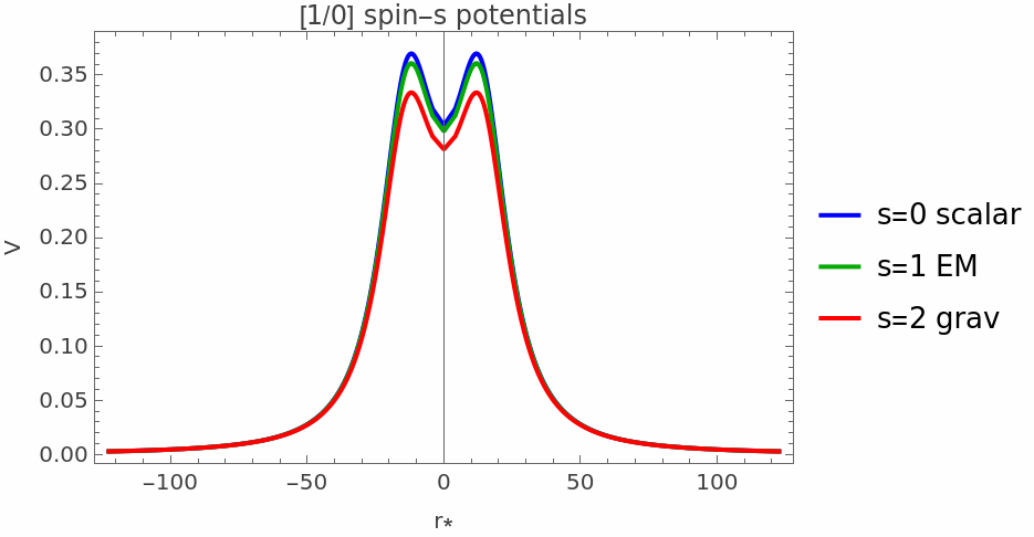
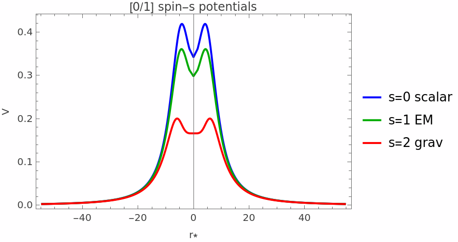
Finally, we examine how the QNM spectrum depends on the spin of the perturbing field, comparing test scalar (), electromagnetic (), and axial gravitational () perturbations through the potential of Eq. (71). The spin- potentials are shown in Fig. 30 for both branches. For the branch the three potentials are nearly degenerate, since the spin-dependent term is small relative to the centrifugal barrier for this broad, slowly varying potential. For the branch the spin dependence is much more pronounced: the scalar barrier is highest and the gravitational barrier is significantly lower and flatter, reflecting the stronger curvature coupling of the more compact geometry.
The corresponding fundamental (, ) frequencies are listed by channel in Table 6. For the branch the frequency decreases only slightly from the scalar to the gravitational channel, by about five percent in the real part. For the branch the variation is far larger: the gravitational real part drops to , roughly thirty percent below the scalar value of , while the damping rates remain comparable across channels. This strong spin dependence of the branch is a direct consequence of the sharper, more spin-sensitive potential, and provides a further observable that distinguishes the two Padé orders.
| Channel | ||
|---|---|---|
| scalar | ||
| EM | ||
| grav |
VII Concluding Remarks
In this work, we constructed traversable wormhole solutions in the linear teleparallel model , with the asymptotically flat, horizon-free redshift function and two Padé-approximated shape functions for the and order. Both reproduce the same first-order Taylor expansion about the throat, satisfy , and meet the flaring-out and admissibility constraints of Sec. III. Because , the field equations reduce to the teleparallel equivalent of general relativity shifted by the constant , and the effective source is identically conserved. Throughout the analysis we adopted the unified parameter set , , , , with for the branch and for the branch.
The energy-condition analysis shows that the tangential null combination is negative at the throat for both orders, so the NEC is violated and the matter is exotic, as required by the flaring-out condition. For the order the throat values are , , and , with the strong-energy combination , so that the radial null channel is satisfied while the tangential channel drives the violation; the NEC, WEC, SEC, and DEC all fail. For the order the energy density at the throat is large and positive, , with and , and the strong-energy combination . Although the energy density is positive here, the negative tangential null combination leaves the NEC violated through the tangential channel, and the WEC, SEC, and DEC fail as well. In both orders the violation is therefore carried entirely by the tangential channel while the radial channel remains satisfied, a feature shared with other anisotropic wormhole constructions in modified gravity. The two orders differ in the radial spread of the violation, with the combinations exhibiting a more pronounced near-throat concentration of exotic matter.
The physical diagnostics confirm viability for both orders. The volume integral quantifier, evaluated over the matched interior region from the throat to the cutoff , is finite and negative, and , so a bounded amount of NEC-violating matter sustains each throat, with the much larger reflecting the deep near-throat concentration of exotic matter in that branch. The TOV analysis gives an exact cancellation , with the hydrostatic force directed outward and the gravitational and anisotropic forces and directed inward, the equilibrium forces being independent of and the branch developing the larger near-throat force magnitudes. The embedding surface and proper radial distance are finite and monotonic in both orders. The gravitational energy and active mass reflect the underlying exotic-matter distribution rather than ordinary positive mass: for the branch the gravitational energy starts at , rises, and then turns negative as the negative-energy-density region dominates, while the active mass dips negative just outside the throat before recovering; for the branch the gravitational energy is negative across most of the range through the geometric factor , even though the energy density is positive, while the active mass grows large and positive. These sign changes are the expected quasilocal-energy signature of NEC-violating matter and are fully consistent with the energy-condition results.
The optical analysis fixes the photon sphere at and the critical impact parameter at . Both quantities depend on the redshift function alone and are therefore identical for the two Padé orders. The shape function controls the bending away from the photon sphere through the factor . The geometry retains a constant deficit , producing broad winding and a non-flat exterior in which is a coordinate quantity. The geometry decays as , giving asymptotic flatness, lensing confined to a compact region, and equal to the true asymptotic impact parameter. The intensity profiles peak at through the photon-ring enhancement, and both the shadow maps and the accretion-disc images show shadow and photon-ring sizes growing monotonically with , with the branch giving a more compact, centrally concentrated crescent at fixed . The embedding diagrams are vertical at the throat in both orders, with the profile flaring more steeply than the pole-free profile, and the timelike rosette orbits precess with the same near-throat rate set by , the branch spreading over larger radii.
The quasinormal-mode analysis gives a positive-definite, symmetric double-barrier potential about the throat for both orders, the barrier taller and sharper and the barrier lower and wider, with peak values and respectively. The peak height decreases with spin following the weighting, the effect being small for the broad barrier and pronounced for the compact barrier. The third-order WKB fundamental scalar frequencies (, ) are for and for respectively. The strictly negative imaginary parts establish linear stability, which is confirmed by the direct time-domain evolution: the ringdown yields a damping rate of from the late-ringdown envelope, in agreement with the WKB value to better than three percent, while the more strongly damped mode rings down within a few cycles so that its fundamental is best quoted from WKB. Both signals cross over at late times to a universal inverse power-law tail. The characteristic frequencies scale approximately as , depend only weakly on , and approach the photon-sphere values in the eikonal limit, with , , , and . The damping rate drops toward zero near , signaling the onset of long-lived, weakly damped oscillations, and the shallow central well, with for both branches, produces a modulated decaying signal rather than a train of discrete echoes.
These results establish the Padé approximation as a practical tool for constructing analytically tractable wormhole geometries in torsion-based gravity. Both Padé-order wormholes in the linear model are stable, traversable configurations sustained by a bounded amount of NEC-violating matter, whose optical and dynamical signatures are testable by horizon-scale very-long-baseline interferometry and gravitational-wave ringdown observations. The asymptotically flat geometry is the more suitable of the two for shadow and lensing observables, since its coordinate impact parameter coincides with the asymptotic one, while the two branches remain clearly distinguishable through their shadow compactness, ringdown damping, Lyapunov exponents, and spin-dependent spectra. Natural extensions include rotating generalizations through a Lense–Thirring or Newman–Janis construction, as well as higher-order Padé approximants. A direct confrontation of the predicted shadow radii and ringdown frequencies with current Event Horizon Telescope and future gravitational-wave detector data remains a compelling observational avenue.
Data availability
No new data are associated with this article.
Acknowledgments
SP acknowledges the support by Chennai Mathematical Institute (CMI). PKS thanks IUCAA, Pune, India, for its assistance through the visiting associateship program.
References
- [1] (2010) Astrophys. J. 725, pp. 787. Cited by: §I.
- [2] (2022) Int. J. Geom. Methods Mod. Phys. 19, pp. 2250170. Cited by: §I, §I.
- [3] (2013) Teleparallel gravity: an introduction. Springer, Dordrecht. Cited by: §II.
- [4] (2016) Int. J. Mod. Phys. D 25, pp. 1650020. Cited by: §I.
- [5] (2013) Int. J. Theor. Phys. 52, pp. 3486. Cited by: §I.
- [6] (1961) J. Math. Anal. Appl. 2, pp. 21. Cited by: §I, §III, §VI.3.
- [7] (2026) Annalen Phys. 538, pp. e00408. Cited by: §IV.3.
- [8] (2021) Eur. Phys. J. C 81, pp. 205. Cited by: §V.2, §V.2, §V.2, §V.3, §V.3, §V.4, §V.4, §V.4.
- [9] (1968) J. Math. Anal. Appl. 21, pp. 469. Cited by: §I.
- [10] (2009) Class. Quantum Grav. 26, pp. 163001. Cited by: §I, §VI.5, §VI.
- [11] (2007) Phys. Rev. D 75, pp. 104016. Cited by: §I.
- [12] (2003) Phys. Rev. D 67, pp. 103009. Cited by: §I.
- [13] (2010) Mod. Phys. Lett. A 25, pp. 2399. Cited by: §I.
- [14] (2018) arXiv:1805.03781 [gr-qc]. Cited by: §V.2, §V.3, §V.3, §VI.3.
- [15] (2001) Gen. Relativ. Gravit. 33, pp. 1535. Cited by: §I.
- [16] (2005) Phys. Rev. D 72, pp. 083003. Cited by: §I.
- [17] (2002) Phys. Rev. D 66, pp. 103001. Cited by: §I, §V.1, §V.2, §V.2, §V.3.
- [18] (1961) Phys. Rev. 124, pp. 925. Cited by: §I.
- [19] (2019) Gravit. Cosmol. 25, pp. 44. Cited by: §I, §I.
- [20] (2020) Echoes in brane worlds: ringing at a black hole–wormhole transition. Phys. Rev. D 101 (6), pp. 064004. Cited by: §I, §VI.7, §VI.7, §VI.
- [21] (2018) Phys. Rev. D 97, pp. 024040. Cited by: §VI.7, §VI.7, §VI.7, §VI.
- [22] (2011) Phys. Rep. 509, pp. 167. Cited by: §I.
- [23] (2020) Mon. Not. R. Astron. Soc. 494, pp. 2576. Cited by: §I.
- [24] (2021) Eur. Phys. J. Plus 136, pp. 167. Cited by: §I, §I.
- [25] (2016) Phys. Rev. Lett. 116, pp. 171101. Cited by: §I, §VI.7, §VI.7, §VI.
- [26] (2009) Phys. Rev. D 79, pp. 064016. Cited by: §VI.1, §VI.4.
- [27] (2017) Eur. Phys. J. C 77, pp. 748. Cited by: §I, §IV.6, §IV.6, §V.4, §V.4, §V.4.
- [28] (1995) Phys. Rev. D 52, pp. 2118. Cited by: §VI.6.
- [29] (2020) Ringing of the regular black hole with asymptotically minkowski core. Class. Quantum Grav. 37 (7), pp. 075014. Cited by: §I.
- [30] (2006) Int. J. Mod. Phys. D 15, pp. 1753. Cited by: §I.
- [31] (1995) Phys. Rev. D 51, pp. 3117. Cited by: §I.
- [32] (1975) Astrophys. J. 202, pp. 788. Cited by: §V.3, §V.3.
- [33] (2019) Phys. Rev. D 100, pp. 083513. Cited by: §I.
- [34] (2007) Phys. Rev. D 76, pp. 024016. Cited by: §VI.7.
- [35] (2020) Phys. Rev. D 101, pp. 104037. Cited by: §I, §V.3.
- [36] (2021) Phys. Rev. D 103, pp. 044007. Cited by: §I, §I, §V.3.
- [37] (2008) Mod. Phys. Lett. A 23, pp. 953. Cited by: §I.
- [38] (1935) Ann. Phys. 2, pp. 242. Cited by: §I.
- [39] (2019) Phys. Rev. D 99, pp. 024051. Cited by: §I.
- [40] (2025) Null geodesics and shadows of slowly rotating wormholes immersed in dark matter halos. arXiv:2509.16739 [gr-qc]. Cited by: §II.
- [41] (2019) Astrophys. J. Lett. 875, pp. L1. Cited by: §V.3, §V.3.
- [42] (2022) Astrophys. J. Lett. 930, pp. L12. Cited by: §V.3, §V.3.
- [43] (2000) Astrophys. J. 528, pp. L13. Cited by: §V.3, §V.3, §V.3.
- [44] (1916) Phys. Z. 17, pp. 448. Cited by: §I.
- [45] (2000) Phys. Rev. D 61, pp. 064021. Cited by: §I.
- [46] (2019) Mod. Phys. Lett. A 34, pp. 1950226. Cited by: §I, §I.
- [47] (2019) Chin. J. Phys. 62, pp. 161. Cited by: §I.
- [48] (2008) Phys. Rev. D 78, pp. 064064. Cited by: §IV.2.
- [49] (2024) East Eur. J. Phys. 1, pp. 112. Cited by: §III.1.
- [50] (2019) Phys. Rev. D 100, pp. 024018. Cited by: §V.3.
- [51] (2014) Phys. Rev. D 89, pp. 103506. Cited by: §I.
- [52] (2022) Phys. Rev. D 105, pp. 084057. Cited by: §I, §I.
- [53] (1994) Phys. Rev. D 49, pp. 883. Cited by: §VI.6, §VI.6.
- [54] (2011) Phys. Rev. D 84, pp. 024020. Cited by: §V.3.
- [55] (2022) Eur. Phys. J. C 82, pp. 1116. Cited by: §IV.1.
- [56] (2012) Int. J. Mod. Phys. D 21, pp. 1250003. Cited by: §I.
- [57] (1987) Phys. Rev. D 35, pp. 3621. Cited by: §I, §VI.1, §VI.2, §VI.2, §VI.2, §VI.5.
- [58] (2022) Nature 612, pp. 51. Cited by: §I.
- [59] (2010) Astrophys. J. 718, pp. 446. Cited by: §V.3, §V.3.
- [60] (2017) Phys. Rev. D 96, pp. 084036. Cited by: §I.
- [61] (2018) Phys. Rev. D 97, pp. 024042. Cited by: §I, §V.1.
- [62] (2006) Class. Quantum Grav. 23, pp. 7111. Cited by: §IV.6.
- [63] (1999) Living Rev. Relativ. 2, pp. 2. Cited by: §I, §VI.
- [64] (2011) Rev. Mod. Phys. 83, pp. 793. Cited by: §I, §VI.1, §VI.1, §VI.2, §VI.3, §VI.4, §VI.5, §VI.5, §VI.
- [65] (2003) Phys. Rev. D 68, pp. 024018. Cited by: §I, §VI.2, §VI.5.
- [66] (2020) Sci. Rep. Phys. Sci. 1, pp. 1. Cited by: §IV.2.
- [67] (2009) Phys. Rev. D 80, pp. 104012. Cited by: §IV.6, §IV.6.
- [68] (2005) Phys. Rev. D 71, pp. 084011. Cited by: §IV.1, §IV.1, §IV.1, §IV.3.
- [69] (1979) Astron. Astrophys. 75, pp. 228. Cited by: §V.3, §V.3, §V.3, §V.3.
- [70] (2020) Int. J. Mod. Phys. A 35, pp. 2050238. Cited by: §I, §I.
- [71] (1988) Am. J. Phys. 56, pp. 395. Cited by: §I, §II, §IV.4.
- [72] (2015) Ann. Phys. 354, pp. 288. Cited by: §I.
- [73] (2012) Phys. Rev. D 85, pp. 107501. Cited by: §I.
- [74] (2017) Phys. Rev. D 95, pp. 104011. Cited by: §I, §V.1, §V.3, §V.4, §V.4.
- [75] (2018) J. Cosmol. Astropart. Phys. 07, pp. 027. Cited by: §I, §V.3, §V.3.
- [76] (2009) Phys. Rev. D 79, pp. 024011. Cited by: §IV.6, §IV.6.
- [77] (2006) Phys. Rev. D 74, pp. 024020. Cited by: §I, §V.2.
- [78] (2023) Chin. J. Phys. 86, pp. 350. Cited by: §I, §I.
- [79] (2023) Phys. Dark Universe 42, pp. 101301. Cited by: §I.
- [80] (2023) Gen. Relativ. Gravit. 55, pp. 45. Cited by: §I, §I.
- [81] (2013) Phys. Rev. D 88, pp. 124019. Cited by: §V.2.
- [82] (2009) Bull. Chelyabinsk State Univ. 8, pp. 54. Cited by: §IV.6.
- [83] (2006) eConf C0602061, pp. 06. Note: [arXiv:hep-th/0601213] Cited by: §I.
- [84] (1973) . In Black Holes (Les Astres Occlus), C. DeWitt and B. S. DeWitt (Eds.), pp. 343. Cited by: §V.3.
- [85] (2015) Phys. Rev. D 92, pp. 044047. Cited by: §I.
- [86] (1939) Phys. Rev. 55, pp. 374. Cited by: §IV.2.
- [87] (1974) Astrophys. J. 191, pp. 499. Cited by: §V.3.
- [88] (1972) Phys. Rev. D 5, pp. 2419. Cited by: §VI.6, §VI.6.
- [89] (2007) Chin. J. Phys. (Taipei) 45, pp. 518. Cited by: §I.
- [90] (2016) Eur. Phys. J. C 76, pp. 246. Cited by: §I.
- [91] (1957) Phys. Rev. 108, pp. 1063. Cited by: §VI.1, §VI.
- [92] (2002) Phys. Rev. D 65, pp. 023001. Cited by: §I.
- [93] (2011) Mod. Phys. Lett. A 26, pp. 1211. Cited by: §I.
- [94] (2023) Chin. J. Phys. 82, pp. 1. Cited by: §I, §I.
- [95] (2019) Mod. Phys. Lett. A 34, pp. 1950224. Cited by: §I.
- [96] (2019) Eur. Phys. J. C 79, pp. 623. Cited by: §I, §I.
- [97] (1992) Gravitational lenses. Springer-Verlag, Berlin. Cited by: §I.
- [98] (1985) Astrophys. J. 291, pp. L33. Cited by: §I, §VI.1, §VI.2.
- [99] (2019) Phys. Lett. B 789, pp. 270. Cited by: §I, §V.1, §V.2.
- [100] (2017) Phys. Rev. D 96, pp. 044037. Cited by: §I, §V.3.
- [101] (2019) J. Cosmol. Astropart. Phys. 07, pp. 028. Cited by: §I, §I, §V.1, §V.1, §V.2, §V.2, §V.2, §V.2, §V.2, §V.3, §V.3, §V.3, §V.4.
- [102] (2018) Phys. Rev. D 98, pp. 024044. Cited by: §V.2, §V.2, §V.2, §V.2, §V.2, §V.3, §V.3, §V.4.
- [103] (1973) Astron. Astrophys. 24, pp. 337. Cited by: §V.3.
- [104] (2015) Astrophys. Space Sci. 357, pp. 85. Cited by: §I.
- [105] (2019) Ann. Phys. 400, pp. 37. Cited by: §I.
- [106] (2021) Phys. Rev. D 104, pp. L081502. Cited by: §I.
- [107] (2023) Chin. J. Phys. 85, pp. 74. Cited by: §I.
- [108] (2026) Int. J. Mod. Phys. A 41, pp. 2650091. Cited by: §IV.1.
- [109] (1998) J. Comput. Appl. Math. 99, pp. 511. Cited by: §I, §VI.3.
- [110] (1980) Phys. Lett. B 91, pp. 99. Cited by: §I.
- [111] (2002) Russ. Math. Surv. 57, pp. 43. Cited by: §I.
- [112] (2025) Nucl. Phys. B 1013, pp. 116838. Cited by: §I, §I.
- [113] (2023) Eur. Phys. J. Plus 138, pp. 539. Cited by: §I, §IV.3.
- [114] (2005) arXiv:gr-qc/0505054. Cited by: §I.
- [115] (2017) Phys. Rev. D 95, pp. 024030. Cited by: §I, §V.2, §V.3.
- [116] (2016) Phys. Rev. D 94, pp. 124001. Cited by: §I, §V.1, §V.1, §V.2, §V.3, §V.4.
- [117] (2019) arXiv:1905.06932 [gr-qc]. Cited by: §V.2, §V.3, §V.3, §VI.3.
- [118] (2023) Class. Quantum Grav. 40, pp. 165007. Cited by: §II, §V.2, §V.2, §V.2, §V.2, §V.2, §V.3, §V.3, §V.3, §V.3.
- [119] (2004) Nuovo Cim. B 119, pp. 489. Cited by: §I.
- [120] (2000) Phys. Rev. D 62, pp. 084003. Cited by: §I, §V.1, §V.2, §V.3.
- [121] (1995) Lorentzian wormholes: from einstein to hawking. AIP Press, Woodbury, NY. Cited by: §I, §IV.1.
- [122] (2017) Eur. Phys. J. Plus 132, pp. 268. Cited by: §I.
- [123] (1970) Phys. Rev. Lett. 24, pp. 737. Cited by: §VI.1, §VI.
- [124] (2016) Eur. Phys. J. C 76, pp. 444. Cited by: §I.