High-Probability Sampled-Data Stabilization of General Nonlinear Stochastic Systems

Kele Sun ^†^†thanks: Research Institute of Intelligent Complex Systems, Fudan University, Shanghai, 200433, China. Yudong Wang ^†^†thanks: Research Institute of Intelligent Complex Systems, Fudan University, Shanghai, 200433, China. Shijie Zhou ^†^†thanks: Corresponding author, Research Institute of Intelligent Complex Systems, Fudan University, Shanghai, 200433, China(). Email: sjzhou14@fudan.edu.cn Wei Lin ^†^†thanks: School of Mathematics Sciences, Fudan University, Shanghai, 200433, China. Xuerong Mao ^†^†thanks: Department of Mathematics and Statistics, University of Strathclyde, G11XH Glasgow, U.K.

Abstract

In this paper, we study sampled-data stabilization of general nonlinear stochastic systems under a local exponential-type Lyapunov condition for the continuous-time closed-loop system. The coefficients are assumed only locally Lipschitz, with neither linear-growth nor Khasminskii-type conditions. Two counterexamples show that almost-sure stabilization is generally unattainable. Instead, given an initial state, we establish exponential stability with arbitrarily high probability under sufficiently fast sampling. Separate methods are developed for $p\geq 2$ and $0<p<2$ , where $p$ is the growth order in the Lyapunov condition. Numerical examples illustrate the results.

1 Introduction

Consider a controlled stochastic differential equation(SDE)

\mathrm{d}\bm{x}_{t}=\bm{f}(\bm{x}_{t},\bm{\alpha}(\bm{x}_{t}))\,\mathrm{d}t+\bm{g}(\bm{x}_{t},\bm{\alpha}(\bm{x}_{t}))\,\mathrm{d}B_{t},

(1)

with feedback $\bm{\alpha}(\cdot)$ to be designed. We seek $\bm{\alpha}(\cdot)$ that stabilizes the closed-loop system. In practice, control signals are held constant over sampling intervals, yielding the sampled-data system

\mathrm{d}\bm{y}_{t}=\bm{f}(\bm{y}_{t},\bm{\alpha}(\bm{y}_{\delta_{t}}))\,\mathrm{d}t+\bm{g}(\bm{y}_{t},\bm{\alpha}(\bm{y}_{\delta_{t}}))\,\mathrm{d}B_{t},\hskip 9.24994pt\delta_{t}=\left\lfloor\frac{t}{\tau}\right\rfloor\tau,

(2)

where $\tau>0$ is the sampling period. Does (2) preserve the stability of (1)?

This is the problem of sampled-data control, which has attracted much attention for reducing computational burden. Mao [21, 22] initiated this direction, followed by numerous studies [5, 9, 16, 17, 24, 30]. Event-triggered stabilization for stochastic systems was studied in [7, 8, 15, 29, 34]. Most of these works assume linear growth conditions on the drift and diffusion coefficients. Several works have addressed highly nonlinear SDEs under Khasminskii-type conditions [3, 4, 10, 23, 28, 27]. Sampled-data homogeneous feedback was used in [31, 32, 33] for stochastic systems with homogeneity degree zero. Recently, [13, 14] established a general framework covering both sampled-data and event-triggered control, with stochastic transmission times and protocols.

Although these works cover a broad class of stochastic systems, they require restrictive conditions that are often hard to verify or too conservative. A natural question arises, can we obtain stability under a weaker local Lipschitz condition? Some progress has been made for ordinary differential equations(ODEs). For ODEs ( $\bm{g}\equiv 0$ in (1), (2)), Lin [12, Theorem 3.1] proved that if (1) is exponentially stable under $\bm{\alpha}$ , then, for each fixed $r>0$ , there exists $\tau^{*}(r)>0$ such that (2) is exponentially stable for all $\|\bm{y}_{0}\|\leq r$ whenever $0<\tau<\tau^{*}(r)$ . The proof only requires $\bm{f}$ and $\bm{\alpha}$ to be locally Lipschitz, without global growth conditions.

In the proof of [12, Theorem 3.1], the authors used a “level set” argument: for any initial value in a compact set, the trajectory stays in a larger bounded set when $\tau$ is enough, where the Lipschitz constant is bounded. This yields a Halanay-type inequality [12, Eq. (82)] and hence the exponential stability.

This raises several questions.

Question 1. Can the result of [12] be extended to SDEs in the almost sure sense?

Answer. No. Even if the initial value lies in a compact set and $\tau$ is arbitrarily small, there is always a nonzero probability that a large Brownian increment $\Delta B_{t}$ drives the state outside the bounded region. To illustrate this more clearly, we provide two counterexamples below; the first is inspired by [31, Example 2.2].

Example 1 (First counterexample: non-explosive continuous case but explosive under sampling).

Consider the one-dimensional stochastic control system

\mathrm{d}x_{t}=\left(x_{t}^{2}+x_{t}^{3}+u_{t}\right)\,\mathrm{d}t+x_{t}^{2}\,\mathrm{d}B_{t},\hskip 9.24994ptx_{0}>0.

(3)

The model combines a superlinear drift $x^{2}+x^{3}$ , which can cause finite-time blow-up (as in fluid collapse and population aggregation), with multiplicative noise $x^{2}\,\mathrm{d}B_{t}$ , whose quadratic intensity produces large fluctuations at high states; $u_{t}$ is an external stabilizing control [6]. With control $u_{t}=\alpha(x_{t})\triangleq-ax_{t}-(k+1)x_{t}^{3}-x_{t}^{2}$ ( $a>0,k>1/2$ ), the closed-loop system becomes $\mathrm{d}x_{t}=(-ax_{t}-kx_{t}^{3})\,\mathrm{d}t+x_{t}^{2}\,\mathrm{d}B_{t}$ , and hence $\mathbb{E}|x_{t}|^{2}\leq|x_{0}|^{2}{\rm e}^{-2at}.$ Thus $\alpha(x)$ stabilizes the system in mean square.

However, under sampled-data control, the same feedback causes explosion in arbitrarily short time with positive probability (proved in Appendix B, Lemma 27), ruling out almost sure stabilization.

Example 2 (Second counterexample: non-explosive, but with some oscillatory divergent paths).

Consider the one-dimensional stochastic control system

\mathrm{d}x_{t}=\left(x_{t}+u_{t}\right)\,\mathrm{d}t+x_{t}^{2}\,\mathrm{d}B_{t},\hskip 9.24994ptx_{0}>0.

This is a controlled CEV-type model whose diffusion term $x^{2}\,\mathrm{d}B_{t}$ makes the volatility grow quadratically with the state, capturing the sharp rise in uncertainty at high state levels. Such models are widely used in asset pricing, risk management, and stochastic optimal control [2]. With feedback $u_{t}=\alpha(x_{t})\triangleq-\kappa x_{t}-x_{t}^{3}$ ( $\kappa>1$ ), the closed-loop system becomes $\mathrm{d}x_{t}=[-(\kappa-1)x_{t}-x_{t}^{3}]\,\mathrm{d}t+x_{t}^{2}\,\mathrm{d}B_{t},$ and hence $\mathbb{E}|x_{t}|^{2}\leq|x_{0}|^{2}{\rm e}^{-2(\kappa-1)t}.$ Thus $\alpha(x)$ stabilizes the system in mean square.

For every $\tau>0$ , the solution exists globally but, with positive probability, diverges at the sampling times while the trajectory crosses zero infinitely often (see Appendix B, Lemma 28), ruling out almost-sure stability.

The above examples show that almost sure stability is generally unattainable for sampled-data systems. Relaxing this to stability with probability $1-\varepsilon$ , we adopt the level-set idea of [12] combined with stopping times; the key is to bound the exit probability from a level set by $\varepsilon$ .

A second question concerns the proof of [12, Theorem 3.1].

Question 2. The proof of [12, Theorem 3.1] employs a Halanay-type inequality [12, Eq. (82)] to derive exponential stability. Can this method be generalized to SDEs?

Answer. Not necessarily. The ODE proof requires a $C^{1}$ Lyapunov function, while Itô’s formula for SDEs requires $C^{2}$ due to the diffusion term. This smoothness may fail even for almost surely exponentially stable systems. Consider the scalar SDE $\mathrm{d}x_{t}=0.2x_{t}\,\mathrm{d}t+x_{t}\,\mathrm{d}B_{t},$ with solution $x_{t}=x_{0}\exp(-0.3t+B_{t})$ . Then $\lim_{t\to\infty}\frac{1}{t}\log|x_{t}|=-0.3\quad\text{a.s.},$ so the system is almost surely exponentially stable. For $V_{p}(x)=|x|^{p}$ , we have $\mathcal{L}V_{p}(x)=\frac{p(p-0.6)}{2}|x|^{p},$ so $\mathbb{E}|x_{t}|^{p}\to 0$ for $p<0.6$ , but $\mathbb{E}|x_{t}|^{p}\to\infty$ for $p>0.6$ . Yet for any $p<0.6$ , $V_{p}$ is not $C^{2}$ at $x=0$ . Thus the Halanay method is inapplicable despite almost sure stability.

Our approach is divided into two cases depending on the regularity of the Lyapunov function.

When a $C^{2}$ Lyapunov function is available, we employ a Halanay-type inequality. However, the stopped process may render the Lyapunov function $U(t)$ (see (7)) discontinuous. We therefore extend the classical Halanay inequality to a generalized version that permits discontinuous functions (Lemma 10).

When no $C^{2}$ Lyapunov function exists, we adopt the comparison method of [21, 22]. On each interval, we construct an auxiliary process, estimate the exit probability from a level set via stopping times, and show that these probabilities form a geometric series whose sum is less than any prescribed $\varepsilon>0$ .

The main contributions are as follows.

•

Unlike other works that focus on SDEs with linear-growth or Khasminskii-type conditions [3, 4, 10, 21, 22, 23, 28], we study sampled-data SDEs with merely locally Lipschitz coefficients and local exponential-type Lyapunov conditions. We prove exponential stabilization with arbitrarily high probability provided the sampling period is sufficiently small for the given initial state (see Theorems 14 and 24).
•

We establish a Halanay-type inequality for possibly discontinuous functions under two one-sided semicontinuity conditions (see Lemma 10), extending the right-continuous result in [27] and applying to the Lyapunov quantity arising from the stopping-time argument for $p\geq 2$ ,where $p$ is the exponent in Assumption 5.
•

For the non- $C^{2}$ case ( $0<p<2$ ), we adopt the comparison method of [21, 22] with stopping times.
•

Two counterexamples demonstrate the sharpness of our results, showing that almost sure stability cannot generally be expected (see Appendix B).

The remainder of this paper is organized as follows. Section 2 presents the necessary preliminaries and assumptions on the SDEs. Sections 3 and 4 contain our main results and their proofs. Section 5 presents two numerical examples to illustrate the high-probability stabilization results. Finally, Section 6 concludes the paper and discusses several directions for future research.

Notations. Throughout this paper, $\mathbb{N}\triangleq\{1,2,\ldots\}$ . For $x\in\mathbb{R}$ , $|x|$ is its absolute value. $\operatorname{sgn}(x)\triangleq 1,0,-1$ for $x>0$ , $x=0$ , and $x<0$ , respectively. For vectors $\bm{x}\in\mathbb{R}^{n}$ or matrices $\bm{A}\in\mathbb{R}^{n\times r}$ , $\|\cdot\|$ denotes the Euclidean or Frobenius norm, and $\bm{A}^{\top}$ is the transpose. For $a,b\in\mathbb{R}\cup\{\pm\infty\}$ , $a\wedge b\triangleq\min\{a,b\}$ , $a\vee b\triangleq\max\{a,b\}$ . For a set $A$ , $A^{c}$ is its complement and $\mathbf{1}_{A}$ its indicator. For integrable $\xi$ and sub- $\sigma$ -algebra $\mathscr{G}\subset\mathscr{F}$ , $\mathbb{E}[\xi\mid\mathscr{G}]$ is the conditional expectation; for $A\in\mathscr{F}$ , $\mathbb{P}(A\mid\mathscr{G})\triangleq\mathbb{E}[\mathbf{1}_{A}\mid\mathscr{G}]$ . The abbreviation $\mathrm{a.s.}$ means almost surely. For differentiable $V:\mathbb{R}^{n}\to\mathbb{R}$ , $V_{\bm{x}}$ and $V_{\bm{x}\bm{x}}$ denote its gradient and Hessian w.r.t. $\bm{x}$ .

2 Problem formulation and preliminaries

Consider Eqs. (1)–(2) with state vectors $\bm{x}_{t},\bm{y}_{t}\in\mathbb{R}^{n}$ . Let $B_{t}$ be a $1$ -dimensional Brownian motion on $\left(\Omega,\mathscr{F},\{\mathscr{F}_{t}\}_{t\geq 0},\mathbb{P}\right)$ with filtration satisfying the usual conditions. The functions $\bm{f}:\mathbb{R}^{n}\times\mathbb{R}^{n}\to\mathbb{R}^{n},\quad\bm{g}:\mathbb{R}^{n}\times\mathbb{R}^{n}\to\mathbb{R}^{n},\quad\bm{\alpha}:\mathbb{R}^{n}\to\mathbb{R}^{n}$ are continuous. We impose the following assumptions.

Assumption 3.

For each $R>0$ , there is $L_{R}>0$ such that for all $\bm{x},\bm{x}^{\prime},\bm{y},\bm{y}^{\prime}\in\mathbb{R}^{n}$ with $\max\{\|\bm{x}\|,\|\bm{x}^{\prime}\|,\|\bm{y}\|,\|\bm{y}^{\prime}\|\}\leq R$ ,

$\displaystyle\\|\bm{f}(\bm{x},\bm{y})-\bm{f}(\bm{x}^{\prime},\bm{y}^{\prime})\\|\vee\\|\bm{g}(\bm{x},\bm{y})-\bm{g}(\bm{x}^{\prime},\bm{y}^{\prime})\\|$	$\displaystyle\leq L_{R}(\\|\bm{x}-\bm{x}^{\prime}\\|+\\|\bm{y}-\bm{y}^{\prime}\\|),$	(4)
$\displaystyle\\|\bm{\alpha}(\bm{x})-\bm{\alpha}(\bm{x}^{\prime})\\|$	$\displaystyle\leq L_{R}\\|\bm{x}-\bm{x}^{\prime}\\|,$	(5)
$\displaystyle\bm{f}(\bm{0},\bm{0})=\bm{0},\hskip 9.24994pt\bm{g}(\bm{0},\bm{0})=\bm{0},\hskip 9.24994pt\bm{\alpha}(\bm{0})=\bm{0}.$		(6)

Remark 4.

By Assumption 3, for every $R>0$ and $p>0$ , there exist constants $M_{f,R}^{(p)},M_{g,R}^{(p)},D_{f,R},D_{g,R},\Lambda_{f,R},\Lambda_{g,R}$ , and $\Gamma_{R}$ such that, whenever $\|\bm{x}\|\vee\|\bm{z}\|\leq R$ ,

		$\displaystyle\\|\bm{f}(\bm{x},\bm{\alpha}(\bm{z}))\\|^{p}\leq M_{f,R}^{(p)}\left(\\|\bm{x}\\|^{p}+\\|\bm{z}\\|^{p}\right),\\|\bm{g}(\bm{x},\bm{\alpha}(\bm{z}))\\|^{p}\leq M_{g,R}^{(p)}\left(\\|\bm{x}\\|^{p}+\\|\bm{z}\\|^{p}\right),$
		$\displaystyle\\|\bm{f}(\bm{x},\bm{\alpha}(\bm{z}))-\bm{f}(\bm{x},\bm{\alpha}(\bm{x}))\\|\leq D_{f,R}\\|\bm{x}-\bm{z}\\|,\\|\bm{g}(\bm{x},\bm{\alpha}(\bm{z}))-\bm{g}(\bm{x},\bm{\alpha}(\bm{x}))\\|\leq D_{g,R}\\|\bm{x}-\bm{z}\\|,$
		$\displaystyle\\|\bm{f}(\bm{x},\bm{\alpha}(\bm{x}))\\|\leq\Gamma_{R}\\|\bm{x}\\|,\\|\bm{g}(\bm{x},\bm{\alpha}(\bm{x}))\\|\leq\Gamma_{R}\\|\bm{x}\\|.$
		$\displaystyle\\|\bm{f}(\bm{x},\bm{\alpha}(\bm{x}))-\bm{f}(\bm{z},\bm{\alpha}(\bm{z}))\\|\leq\Lambda_{f,R}\\|\bm{x}-\bm{z}\\|,\\|\bm{g}(\bm{x},\bm{\alpha}(\bm{x}))-\bm{g}(\bm{z},\bm{\alpha}(\bm{z}))\\|\leq\Lambda_{g,R}\\|\bm{x}-\bm{z}\\|$

We impose a local exponential-type Lyapunov condition on system (1).

Assumption 5.

There exist constants $p>0$ , $c_{1}>0$ , and a function $V:\mathbb{R}^{n}\to[0,\infty)$ such that:

(i)

$V(\bm{0})=0$ , $V$ is continuous on $\mathbb{R}^{n}$ , and $V\in C^{2}(\mathbb{R}^{n}\setminus\{\bm{0}\};[0,\infty))$ . Moreover, if $p\geq 2$ , then $V\in C^{2}(\mathbb{R}^{n})$ ;
(ii)

for all $\bm{x}\in\mathbb{R}^{n}\setminus\{\bm{0}\}$ , $V(\bm{x})\geq c_{1}\|\bm{x}\|^{p},\mathcal{L}V(\bm{x})<0;$
(iii)

for every $R>0$ , there exists $\lambda_{R}>0$ such that for all $0<\|\bm{x}\|\leq R$ , $\mathcal{L}V(\bm{x})\leq-\lambda_{R}V(\bm{x});$
(iv)

for every $R>0$ , there exist constants $c_{2,R},c_{3,R}>0$ such that for all $0<\|\bm{x}\|\leq R$ , $\|V_{\bm{x}}(\bm{x})\|\leq c_{2,R}\|\bm{x}\|^{p-1},\|V_{\bm{x}\bm{x}}(\bm{x})\|\leq c_{3,R}\|\bm{x}\|^{p-2}.$

Here, for $\bm{x}\neq\bm{0}$ , the infinitesimal generator $\mathcal{L}V$ is defined by

\mathcal{L}V(\bm{x})\triangleq V_{\bm{x}}(\bm{x})^{\top}\bm{f}(\bm{x},\bm{\alpha}(\bm{x}))+\frac{1}{2}\bm{g}(\bm{x},\bm{\alpha}(\bm{x}))^{\top}V_{\bm{x}\bm{x}}(\bm{x})\,\bm{g}(\bm{x},\bm{\alpha}(\bm{x})).

Remark 6.

By the stochastic LaSalle invariance principle [18, 19], (ii) implies $\bm{x}_{t}\to\bm{0}$ a.s. for (1), while (iii) yields exponential convergence [20, Chapter 4, Theorem 3.3], essential for the stability of (2). For ODEs ( $\bm{g}\equiv 0$ ), exponential stability of (1) yields semiglobal stability of (2), whereas asymptotic stability yields only practical stability; see [12, 25].

Remark 7.

The canonical choice $V(\bm{x})=\|\bm{x}\|^{p}$ satisfies the regularity and derivative-growth requirements in Assumption 5(i) and (iv). Condition (iii) requires only local exponential decay, not a uniform global rate, thus extending [20, Chapter 4, Theorem 4.4]. Indeed, for $\dot{x}=f(x)$ , where $f(x)=-x$ for $|x|\leq 1$ and $f(x)=-\operatorname{sgn}(x)$ otherwise, $V(x)=x^{2}$ satisfies (iii) and (iv), but $\dot{V}(x)\leq-\lambda V(x)$ fails globally for every $\lambda>0$ .

For each $R>\|\bm{y}_{0}\|$ , define $\rho_{R}\triangleq\inf\{t\geq 0:\|\bm{y}_{t}\|\geq R\}$ , with $\inf\emptyset=+\infty$ . The limit $\rho_{\infty}\triangleq\lim_{R\to+\infty}\rho_{R}$ is well defined, and by standard arguments the solution $\bm{y}_{t}$ to Eq. (2) exists on $[0,\rho_{\infty})$ .

In the following, we discuss the stability of (2) separately for the two cases $p\geq 2$ and $p\in(0,2)$ .

3 The case $p\geq 2$ : a Halanay-type approach

In this section, we show that for the case $p\geq 2$ , the stability can be proved by a direct application of the Halanay-type inequality.

Fix an arbitrary $R>\|\bm{y}_{0}\|$ . For $t\geq 0$ , define

U(t)\triangleq\mathbb{E}\left[V(\bm{y}_{t})\cdot\mathbf{1}_{\{t<\rho_{R}\}}\right].

(7)

We extend it to $[-\tau,0]$ by $U(t)=U(0)$ for $t\in[-\tau,0]$ .

3.1 Preliminary estimates and lemmas

We first collect several preliminary estimates and lemmas that will be used in the subsequent Halanay-type analysis.

Lemma 8.

Suppose that Assumptions 3 and 5 hold. Then,

\mathbb{E}\left[\|\bm{y}_{t}-\bm{y}_{\delta_{t}}\|^{p}\cdot\mathbf{1}_{\{t<\rho_{R}\}}\right]\leq K(R,p,\tau)\sup_{\delta_{t}\leq r\leq t}U(r),\forall t\geq 0,

(8)

where

K(R,p,\tau)\triangleq\frac{2^{p}}{c_{1}}\left[M_{f,R}^{(p)}\tau^{p}+\left(\frac{p(p-1)}{2}\right)^{p/2}M_{g,R}^{(p)}\tau^{p/2}\right].

(9)

Proof.

Integrating (2) over $[\delta_{t}\wedge\rho_{R},t\wedge\rho_{R}]$ yields

\bm{y}_{t\wedge\rho_{R}}-\bm{y}_{\delta_{t}\wedge\rho_{R}}=\int_{\delta_{t}}^{t}\bm{f}(\bm{y}_{s},\bm{\alpha}(\bm{y}_{\delta_{s}}))\cdot\mathbf{1}_{\{s<\rho_{R}\}}\,\mathrm{d}s+\int_{\delta_{t}}^{t}\bm{g}(\bm{y}_{s},\bm{\alpha}(\bm{y}_{\delta_{s}}))\cdot\mathbf{1}_{\{s<\rho_{R}\}}\,\mathrm{d}B_{s}.

Multiplying both sides by $\mathbf{1}_{\{t<\rho_{R}\}}$ and noting that $\left(\bm{y}_{t\wedge\rho_{R}}-\bm{y}_{\delta_{t}\wedge\rho_{R}}\right)\cdot\mathbf{1}_{\{t<\rho_{R}\}}=\left(\bm{y}_{t}-\bm{y}_{\delta_{t}}\right)\cdot\mathbf{1}_{\{t<\rho_{R}\}},$ we obtain, by Hölder’s inequality and [20, Chapter 1, Theorem 7.1],

		$\displaystyle\mathbb{E}\left[\\|\bm{y}_{t}-\bm{y}_{\delta_{t}}\\|^{p}\cdot\mathbf{1}_{\{t<\rho_{R}\}}\right]\leq 2^{p-1}(t-\delta_{t})^{p-1}\int_{\delta_{t}}^{t}\mathbb{E}\left[\\|\bm{f}(\bm{y}_{s},\bm{\alpha}(\bm{y}_{\delta_{s}}))\\|^{p}\cdot\mathbf{1}_{\{s<\rho_{R}\}}\right]\mathrm{d}s$
		$\displaystyle+2^{p-1}\left(\frac{p(p-1)}{2}\right)^{p/2}(t-\delta_{t})^{p/2-1}\int_{\delta_{t}}^{t}\mathbb{E}\left[\\|\bm{g}(\bm{y}_{s},\bm{\alpha}(\bm{y}_{\delta_{s}}))\\|^{p}\cdot\mathbf{1}_{\{s<\rho_{R}\}}\right]\mathrm{d}s.$

On $\{s<\rho_{R}\}$ , one has $\|\bm{y}_{s}\|\vee\|\bm{y}_{\delta_{s}}\|\leq R$ . Moreover, $\delta_{s}=\delta_{t}$ for almost every $s\in[\delta_{t},t]$ . Therefore, by Assumption 5(ii) and Remark 4,

	$\displaystyle\mathbb{E}\left[\\|\bm{f}(\bm{y}_{s},\bm{\alpha}(\bm{y}_{\delta_{s}}))\\|^{p}\cdot\mathbf{1}_{\{s<\rho_{R}\}}\right]$	$\displaystyle\leq\frac{M_{f,R}^{(p)}}{c_{1}}\left[U(s)+U(\delta_{s})\right],$
	$\displaystyle\mathbb{E}\left[\\|\bm{g}(\bm{y}_{s},\alpha(\bm{y}_{\delta_{s}}))\\|^{p}\cdot\mathbf{1}_{\{s<\rho_{R}\}}\right]$	$\displaystyle\leq\frac{M_{g,R}^{(p)}}{c_{1}}\left[U(s)+U(\delta_{s})\right].$

Substitution of these estimates gives

		$\displaystyle\mathbb{E}\left[\\|\bm{y}_{t}-\bm{y}_{\delta_{t}}\\|^{p}\cdot\mathbf{1}_{\{t<\rho_{R}\}}\right]$
	$\displaystyle\leq$	$\displaystyle\frac{2^{p}}{c_{1}}\left[M_{f,R}^{(p)}(t-\delta_{t})^{p}+\left(\frac{p(p-1)}{2}\right)^{p/2}M_{g,R}^{(p)}(t-\delta_{t})^{p/2}\right]\sup_{\delta_{t}\leq r\leq t}U(r).$

And by $t-\delta_{t}\leq\tau$ , we prove (8).

Lemma 9.

Suppose that Assumptions 3 and 5 hold. Then, for every $R>0$ and all $\bm{x},\bm{z}\in\mathbb{R}^{n}$ satisfying $\|\bm{x}\|\vee\|\bm{z}\|\leq R$ , one has

V_{\bm{x}}(\bm{x})\bm{f}(\bm{x},\bm{\alpha}(\bm{z}))+\frac{1}{2}\bm{g}^{\top}(\bm{x},\bm{\alpha}(\bm{z}))V_{\bm{x}\bm{x}}(\bm{x})\bm{g}(\bm{x},\bm{\alpha}(\bm{z}))\leq-\frac{\lambda_{R}}{2}V(\bm{x})+H(R,p)\|\bm{x}-\bm{z}\|^{p},

(10)

where $H(R,p)\triangleq A_{R}\left(\frac{4A_{R}}{c_{1}\lambda_{R}}\right)^{p-1}+B_{R}\left(\frac{4B_{R}}{c_{1}\lambda_{R}}\right)^{\frac{p-2}{2}},A_{R}\triangleq c_{2,R}D_{f,R}+c_{3,R}\Gamma_{R}D_{g,R},B_{R}\triangleq\frac{1}{2}c_{3,R}D_{g,R}^{2}.$

Proof.

Denote the left-hand side of (10) by $\mathcal{L}_{\bm{z}}V(\bm{x})$ and set $d=\|\bm{x}-\bm{z}\|$ . Adding and subtracting the corresponding closed-loop terms and using Assumptions 5, we obtain

	$\displaystyle\mathcal{L}_{\bm{z}}V(\bm{x})$	$\displaystyle\leq-\lambda_{R}V(\bm{x})+c_{2,R}D_{f,R}\\|\bm{x}\\|^{p-1}d+\frac{1}{2}c_{3,R}\\|\bm{x}\\|^{p-2}\left(2\Gamma_{R}D_{g,R}\\|\bm{x}\\|d+D_{g,R}^{2}d^{2}\right)$
		$\displaystyle=-\lambda_{R}V(\bm{x})+A_{R}\\|\bm{x}\\|^{p-1}d+B_{R}\\|\bm{x}\\|^{p-2}d^{2}.$

By Young’s inequality, $A_{R}\|\bm{x}\|^{p-1}d\leq\frac{c_{1}\lambda_{R}}{4}\|\bm{x}\|^{p}+A_{R}\left(\frac{4A_{R}}{c_{1}\lambda_{R}}\right)^{p-1}d^{p},B_{R}\|\bm{x}\|^{p-2}d^{2}\leq\frac{c_{1}\lambda_{R}}{4}\|\bm{x}\|^{p}+B_{R}\left(\frac{4B_{R}}{c_{1}\lambda_{R}}\right)^{\frac{p-2}{2}}d^{p}.$ The conclusion follows from $V(\bm{x})\geq c_{1}\|\bm{x}\|^{p}$ .

We next establish a Halanay inequality for our analysis. Baker and Buckwar [1] used such an argument for SDEs with delays. Xu, Mao, and Yin [27] extended it to right-continuous functions for hybrid systems. However, since our $U(t)$ has specific jumps, we impose assumption (11) to rule out upward jumps and ensure the estimates hold across discontinuities. Lemma 10 is then established; its proof is deferred to Appendix A.

Lemma 10.

Let $\tau>0$ and $a>b\geq 0$ . Let $\Phi:[-\tau,\infty)\longrightarrow[0,\infty)$ be locally bounded. Assume that, for every $t\geq 0$ ,

\limsup_{s\to t^{+}}\Phi(s)\leq\Phi(t)\leq\liminf_{s\to t^{-}}\Phi(s),

(11)

and that the upper right Dini derivative satisfies

D^{+}\Phi(t)\leq-a\Phi(t)+b\sup_{-\tau\leq\theta\leq 0}\Phi(t+\theta),\quad t\geq 0,

(12)

where $D^{+}\Phi(t)\triangleq\limsup_{h\to 0^{+}}\frac{\Phi(t+h)-\Phi(t)}{h}$ . Then there exists a unique $\mu>0$ satisfying $\mu=a-b{\mathrm{e}}^{\mu\tau}$ , and for $t\geq 0$ , $\Phi(t)\leq{\mathrm{e}}^{-\mu t}\sup_{-\tau\leq s\leq 0}\Phi(s)$ .

3.2 A Halanay-type inequality and related estimates

Lemma 11.

Let Assumptions 3 and 5 hold. Suppose that $H(R,p)K(R,p,\tau)$ $<\frac{\lambda_{R}}{2}$ . Let $\mu_{R}(\tau)>0$ be the unique solution of

\mu_{R}(\tau)+H(R,p)K(R,p,\tau){\mathrm{e}}^{\mu_{R}(\tau)\tau}=\frac{\lambda_{R}}{2}.

(13)

Then, for every $t\geq 0$ , $U(t)\leq V(\bm{y}_{0}){\mathrm{e}}^{-\mu_{R}(\tau)t}$ .

Proof.

Since $V$ is continuous and hence bounded on $\|\bm{y}_{t}\|\leq R$ , the dominated convergence theorem and the continuity of $\bm{y}_{t}$ yield $\lim_{s\to t+}U(s)=U(t)$ and $\lim_{s\to t-}U(s)=\lim_{s\to t-}\mathbb{E}\left[V(\bm{y}_{s})\cdot\mathbf{1}_{\{s<\rho_{R}\}}\right]=\mathbb{E}\left[V(\bm{y}_{t})\cdot\mathbf{1}_{\{t\leq\rho_{R}\}}\right].$ Consequently, $\lim_{s\to t-}U(s)-U(t)=\mathbb{E}\left[V(\bm{y}_{t})\cdot\mathbf{1}_{\{\rho_{R}=t\}}\right]\geq 0.$ Thus, $U$ is right-continuous and can only have downward jumps on the left. Next we establish a Halanay-type inequality for $U(t)$ . For every $h>0$ ,

	$\displaystyle\frac{U(t+h)-U(t)}{h}={}$	$\displaystyle\frac{1}{h}\mathbb{E}\left[V(\bm{y}_{(t+h)\wedge\rho_{R}})-V(\bm{y}_{t\wedge\rho_{R}})\right]-\frac{1}{h}\mathbb{E}\left[V(\bm{y}_{\rho_{R}})\cdot\mathbf{1}_{\{t<\rho_{R}\leq t+h\}}\right]$
	$\displaystyle\leq{}$	$\displaystyle\frac{1}{h}\mathbb{E}\left[V(\bm{y}_{(t+h)\wedge\rho_{R}})-V(\bm{y}_{t\wedge\rho_{R}})\right].$		(14)

Applying Itô’s formula to the stopped process gives

V(\bm{y}_{(t+h)\wedge\rho_{R}})-V(\bm{y}_{t\wedge\rho_{R}})=\int_{t}^{t+h}\mathbf{1}_{\{s<\rho_{R}\}}\mathcal{L}_{\bm{y}_{\delta_{s}}}V(\bm{y}_{s})\,{\mathrm{d}}s+\int_{t}^{t+h}\mathbf{1}_{\{s<\rho_{R}\}}\cdots\,{\mathrm{d}}B_{s},

Taking expectations and using Lemma 9, we obtain from (14) that

\displaystyle\frac{U(t+h)-U(t)}{h}\leq\frac{1}{h}\int_{t}^{t+h}\left[-\frac{\lambda_{R}}{2}U(s)+H(R,p)\mathbb{E}\left(\|\bm{y}_{s}-\bm{y}_{\delta_{s}}\|^{p}\cdot\mathbf{1}_{\{s<\rho_{R}\}}\right)\right]\,ds.

(15)

By (8) and $\delta_{s}\geq(s-\tau)\vee 0$ and $U$ has been extended to $[-\tau,0]$ , (15) yields

\frac{U(t+h)-U(t)}{h}\leq\frac{1}{h}\int_{t}^{t+h}\left[-\frac{\lambda_{R}}{2}U(s)+H(R,p)K(R,p,\tau)\sup_{s-\tau\leq r\leq s}U(r)\right]\,{\mathrm{d}}s.

Letting $h\to 0+$ and using the right-continuity of $U$ , we obtain

D^{+}U(t)\leq-\frac{\lambda_{R}}{2}U(t)+H(R,p)K(R,p,\tau)\sup_{t-\tau\leq r\leq t}U(r).

By Lemma 10, we obtain the desired result.

Lemma 12.

Let $R>\|\bm{y}_{0}\|$ , and suppose that the assumptions of Lemma 11 hold. Then

\mathbb{P}(\rho_{R}<+\infty)\leq\left[1+H(R,p)K(R,p,\tau)\frac{\tau}{1-e^{-\mu_{R}(\tau)\tau}}\right]\frac{V(\bm{y}_{0})}{c_{1}R^{p}}.

Proof.

Applying Itô’s formula to $V(\bm{y}_{t\wedge\rho_{R}})$ and using Lemma 9, we obtain

	$\displaystyle\mathbb{E}V(\bm{y}_{t\wedge\rho_{R}})\leq{}$	$\displaystyle V(\bm{y}_{0})+\int_{0}^{t}\left[-\frac{\lambda_{R}}{2}U(s)+H(R,p)\mathbb{E}\left(\\|\bm{y}_{s}-\bm{y}_{\delta_{s}}\\|^{p}\cdot\mathbf{1}_{\{s<\rho_{R}\}}\right)\right]{\rm d}s$
	$\displaystyle\leq{}$	$\displaystyle V(\bm{y}_{0})+H(R,p)K(R,p,\tau)\int_{0}^{t}\sup_{\delta_{s}\leq r\leq s}U(r)\,{\rm d}s.$

By Lemma 11, for $\delta_{s}\leq r\leq s$ , $U(r)\leq V(\bm{y}_{0})e^{-\mu_{R}(\tau)r}\leq V(\bm{y}_{0})e^{-\mu_{R}(\tau)\delta_{s}}.$ Hence,

	$\displaystyle\mathbb{E}V(\bm{y}_{t\wedge\rho_{R}})$	$\displaystyle\leq V(\bm{y}_{0})+H(R,p)K(R,p,\tau)V(\bm{y}_{0})\int_{0}^{t}e^{-\mu_{R}(\tau)\delta_{s}}\,{\mathrm{d}}s$
		$\displaystyle\leq V(\bm{y}_{0})+H(R,p)K(R,p,\tau)V(\bm{y}_{0})\sum_{n=0}^{\infty}\int_{n\tau}^{(n+1)\tau}e^{-\mu_{R}(\tau)n\tau}\,{\mathrm{d}}s$
		$\displaystyle=\left[1+H(R,p)K(R,p,\tau)\frac{\tau}{1-e^{-\mu_{R}(\tau)\tau}}\right]V(\bm{y}_{0}).$

On the other hand, $c_{1}R^{p}\mathbb{P}(\rho_{R}\leq t)\leq\mathbb{E}\left[V(\bm{y}_{\rho_{R}})\cdot\mathbf{1}_{\{\rho_{R}\leq t\}}\right]\leq\mathbb{E}V(\bm{y}_{t\wedge\rho_{R}})$ . Substituting this into the last inequality and letting $t\to+\infty$ yields the desired assertion.

3.3 Almost sure exponential stability on a non-exit event

In this subsection, we establish almost sure exponential stability on the non-exit event $\{\rho_{R}=+\infty\}.$

Lemma 13.

Suppose that the assumptions of Lemma 11 hold. Then

\limsup_{t\to+\infty}\frac{1}{t}\log\|\bm{y}_{t}\|\leq-\frac{\mu_{R}(\tau)}{p}\hskip 9.24994pt\text{{\rm a.s.} on }\{\rho_{R}=+\infty\}.

(16)

Proof.

By Lemma 11 and $V(\bm{x})\geq c_{1}\|\bm{x}\|^{p}$ ,

\mathbb{E}\left[\|\bm{y}_{t}\|^{p}\cdot\mathbf{1}_{\{t<\rho_{R}\}}\right]\leq\frac{V(\bm{y}_{0})}{c_{1}}e^{-\mu_{R}(\tau)t}.

(17)

For $a\in(0,1]$ , define $\zeta_{a}\triangleq\inf\{t\geq 0:\|\bm{y}_{t}\|\geq a\}$ . Applying Itô’s formula to $\|\bm{y}_{t\wedge\zeta_{a}}\|^{p}$ on $[0,\tau]$ , taking expectation and using $\|\bm{y}_{0}\|\vee\|\bm{y}_{s}\|<a\leq 1$ on $\{s<\zeta_{a}\}$ , the local Lipschitz conditions imply that there exists a constant $C>0$ such that

		$\displaystyle\mathbb{E}\\|\bm{y}_{t\wedge\zeta_{a}}\\|^{p}=\\|\bm{y}_{0}\\|^{p}+\int_{0}^{t}\mathbb{E}\bigl[\bigl(p\\|\bm{y}_{s}\\|^{p-2}\bm{y}_{s}^{\top}\bm{f}(\bm{y}_{s},\bm{\alpha}(\bm{y}_{0}))+\frac{p}{2}\\|\bm{y}_{s}\\|^{p-2}\\|\bm{g}(\bm{y}_{s},\bm{\alpha}(\bm{y}_{0}))\\|^{2}$
		$\displaystyle+\frac{p(p-2)}{2}\\|\bm{y}_{s}\\|^{p-4}\left(\bm{y}_{s}^{\top}\bm{g}(\bm{y}_{s},\bm{\alpha}(\bm{y}_{0}))\right)^{2}\bigr)\cdot\mathbf{1}_{\{s<\zeta_{a}\}}\bigr]\mathrm{d}s$
		$\displaystyle\leq\\|\bm{y}_{0}\\|^{p}+C\int_{0}^{t}\mathbb{E}\left[\left(\\|\bm{y}_{s}\\|^{p}+\\|\bm{y}_{0}\\|^{p}\right)\cdot\mathbf{1}_{\{s<\zeta_{a}\}}\right]\mathrm{d}s\leq(1+Ct)\\|\bm{y}_{0}\\|^{p}+C\int_{0}^{t}\mathbb{E}\\|\bm{y}_{s\wedge\zeta_{a}}\\|^{p}\,\mathrm{d}s.$

The Gronwall’s inequality gives $\mathbb{E}\|\bm{y}_{\tau\wedge\zeta_{a}}\|^{p}\leq(1+C\tau)e^{C\tau}\|\bm{y}_{0}\|^{p}.$ Consequently,

\mathbb{P}\left(\sup_{0\leq t\leq\tau}\|\bm{y}_{t}\|\geq a\right)=\mathbb{P}(\zeta_{a}\leq\tau)\leq\frac{1}{a^{p}}\mathbb{E}\|\bm{y}_{\tau\wedge\zeta_{a}}\|^{p}\leq\frac{(1+C\tau)e^{C\tau}}{a^{p}}\|\bm{y}_{0}\|^{p}.

(18)

Shifting (18) to $[k\tau,(k+1)\tau]$ , multiplying $\bm{1}_{k\tau<\rho_{R}}$ , choosing $a_{\epsilon}=\exp\left\{-\frac{\mu_{R}(\tau)-\varepsilon}{p}\tau\right\}$ for $\epsilon>0$ sufficiently small, taking expectation and using (17) gives

		$\displaystyle\sum_{k=1}^{+\infty}\mathbb{P}\left(\sup_{t\in[k\tau,(k+1)\tau]}\\|\bm{y}_{t}\\|\geq a_{\epsilon}^{k};k\tau<\rho_{R}\right)\leq(1+C\tau)e^{C\tau}\sum_{k=1}^{+\infty}\displaystyle\frac{\mathbb{E}\left[\\|\bm{y}_{k\tau}\\|^{p};k\tau<\rho_{R}\right]}{a_{\epsilon}^{kp}}$
		$\displaystyle\leq\frac{(1+C\tau){\rm e}^{c\tau}V(\bm{y_{0}})}{c_{1}}\sum_{k=1}^{+\infty}{\rm e}^{-\epsilon k\tau}<+\infty.$

By the Borel–Cantelli lemma, $\limsup_{t\to\infty}\displaystyle\frac{\log\|\bm{y}_{t}\|}{t}\leq-\frac{\mu_{R}(\tau)-\varepsilon}{p}\hskip 9.24994pt\text{a.s. on }\{\rho_{R}=\infty\}.$ Letting $\epsilon\to 0+$ yields (16).

3.4 Parameter selection and main result

By suitably choosing the parameters, we establish the main result of this section.

Theorem 14.

Suppose that the assumptions of Lemma 11 hold. Given $\varepsilon\in(0,1)$ and $\bm{y}_{0}\in\mathbb{R}^{n}\backslash\{\bm{0}\}$ , there exists $\tau^{*}=\tau^{*}(V(\bm{y}_{0}),\varepsilon)>0$ such that for $\tau\in(0,\tau^{*})$ ,

\mathbb{P}\left(\{\rho_{\infty}=+\infty\}\cap\left\{\limsup_{t\to+\infty}\frac{1}{t}\log\|\bm{y}_{t}\|<0\right\}\right)\geq 1-\varepsilon.

(19)

Proof.

Fix $\varepsilon\in(0,1)$ and $\bm{y}_{0}\in\mathbb{R}^{n}\setminus\{\bm{0}\}$ . We first choose $R$ such that

R>\max\left\{\|\bm{y}_{0}\|,\left(\frac{2V(\bm{y}_{0})}{c_{1}\varepsilon}\right)^{1/p}\right\}.

(20)

We then choose $\tau^{*}>0$ sufficiently small such that, for every $\tau\in(0,\tau^{*})$ ,

H(R,p)K(R,p,\tau)<\frac{\lambda_{R}}{2},\hskip 9.24994pt1+H(R,p)K(R,p,\tau)\frac{\tau}{1-\mathrm{e}^{-\mu_{R}(\tau)\tau}}<2.

(21)

We verify that such a $\tau^{*}$ exists. Since $H(R,p)K(R,p,\tau)=O(\tau^{p/2})\to 0$ as $\tau\to 0+$ . Thus, the first inequality holds for all sufficiently small $\tau>0$ . Moreover, it follows from (13) that $\mu_{R}(\tau)\longrightarrow\frac{\lambda_{R}}{2}\text{as }\tau\to 0^{+}.$ Consequently, $\frac{\tau}{1-\mathrm{e}^{-\mu_{R}(\tau)\tau}}\to\frac{2}{\lambda_{R}},$ and hence $H(R,p)K(R,p,\tau)\frac{\tau}{1-\mathrm{e}^{-\mu_{R}(\tau)\tau}}=O(\tau^{p/2})\to 0.$ Therefore, the second inequality also holds for all sufficiently small $\tau>0$ . By Lemma 12, (20) and (21) give

\mathbb{P}(\rho_{R}<+\infty)\leq\left[1+H(R,p)K(R,p,\tau)\frac{\tau}{1-\mathrm{e}^{-\mu_{R}(\tau)\tau}}\right]\frac{V(\bm{y}_{0})}{c_{1}R^{p}}<\frac{2V(\bm{y}_{0})}{c_{1}R^{p}}<\varepsilon.

Therefore, $\mathbb{P}(\rho_{R}=+\infty)\geq 1-\varepsilon$ . By Lemma 13, almost surely on $\{\rho_{R}=+\infty\}$ , $\limsup_{t\to+\infty}\frac{1}{t}\log\|\bm{y}_{t}\|\leq-\frac{\mu_{R}(\tau)}{p}<0.$ Since $\{\rho_{R}=+\infty\}\subset\{\rho_{\infty}=+\infty\},$ we have

\mathbb{P}\left(\{\rho_{\infty}=+\infty\}\cap\left\{\limsup_{t\to+\infty}\frac{1}{t}\log\|\bm{y}_{t}\|<0\right\}\right)\geq\mathbb{P}(\rho_{R}=+\infty)\geq 1-\varepsilon,

which proves (19).

4 The case $0<p<2$ : a comparison approach via an auxiliary system

In this section, for the case $p\in(0,2)$ , we use the comparison method developed in [21, 22].

4.1 Preliminary estimates

Lemma 15.

Suppose that Assumption 3 and 5 hold. For every $R>0$ and $\bm{x},\bm{y}\in\mathbb{R}^{n}$ satisfying $\|\bm{x}\|\vee\|\bm{y}\|\leq R,$ the following estimates hold.

If $0<p\leq 1$ , then

|V(\bm{x})-V(\bm{y})|\leq\frac{2^{1-p}c_{2,R}}{p}\|\bm{x}-\bm{y}\|^{p}.

(22)

If $1<p<2$ , then

|V(\bm{x})-V(\bm{y})|\leq c_{2,R}\left(\|\bm{x}\|^{p-1}+\|\bm{y}\|^{p-1}\right)\|\bm{x}-\bm{y}\|.

(23)

In this case, for every $\varkappa\in(0,1)$ ,

V(\bm{x})\leq\frac{1+\varkappa}{1-\varkappa}V(\bm{y})+\frac{2(p-1)^{p-1}c_{2,R}^{p}}{p^{p}\varkappa^{p-1}(1-\varkappa)c_{1}^{p-1}}\|\bm{x}-\bm{y}\|^{p}.

(24)

Proof.

If $\bm{x}=\bm{y}$ , the assertion is trivial. Suppose that $\bm{x}\neq\bm{y}$ . By the integral form of the mean value theorem and Assumption 5(iv),

|V(\bm{x})-V(\bm{y})|\leq c_{2,R}\|\bm{x}-\bm{y}\|\int_{0}^{1}\|\bm{y}+\theta(\bm{x}-\bm{y})\|^{p-1}\,\mathrm{d}\theta.

If the line segment joining $\bm{x}$ and $\bm{y}$ passes through the origin, the above inequality follows by splitting the segment at the origin and using a limiting argument. We first consider $0<p<1$ . Since $p-1<0$ ,

		$\displaystyle\int_{0}^{1}\\|\bm{y}+\theta(\bm{x}-\bm{y})\\|^{p-1}\,\mathrm{d}\theta\leq\int_{0}^{1}\left\|\left(\bm{y}+\theta(\bm{x}-\bm{y})\right)^{\top}\frac{\bm{x}-\bm{y}}{\\|\bm{x}-\bm{y}\\|}\right\|^{p-1}\,\mathrm{d}\theta=\\|\bm{x}-\bm{y}\\|^{p-1}\cdot$
		$\displaystyle\int_{0}^{1}\left\|\frac{\bm{y}^{\top}(\bm{x}-\bm{y})}{\\|\bm{x}-\bm{y}\\|^{2}}+\theta\right\|^{p-1}\,\mathrm{d}\theta\leq\\|\bm{x}-\bm{y}\\|^{p-1}\sup_{a\in\mathbb{R}}\int_{a}^{a+1}\|u\|^{p-1}\,\mathrm{d}u=\frac{2^{1-p}}{p}\\|\bm{x}-\bm{y}\\|^{p-1}.$

Here the last equality follows because $|u|^{p-1}$ is even and decreasing with respect to $|u|$ . Combining this estimate with the preceding inequality proves (22) for $0<p<1$ .

If $p=1$ , Assumption 5 directly gives (22).

Now we consider $1<p<2$ . Since $p-1\in(0,1)$ , for $\theta\in[0,1]$ , $\|\bm{y}+\theta(\bm{x}-\bm{y})\|^{p-1}\leq\|\bm{x}\|^{p-1}+\|\bm{y}\|^{p-1}$ . Together with the integral mean-value estimate, this proves (23). Finally, Young’s inequality and $V(\bm{z})\geq c_{1}\|\bm{z}\|^{p}$ from Assumption 5 give, for $\bm{z}=\bm{x},\bm{y}$ ,

	$\displaystyle c_{2,R}\\|\bm{z}\\|^{p-1}\\|\bm{x}-\bm{y}\\|$	$\displaystyle\leq\varkappa c_{1}\\|\bm{z}\\|^{p}+\frac{(p-1)^{p-1}c_{2,R}^{p}}{p^{p}\varkappa^{p-1}c_{1}^{p-1}}\\|\bm{x}-\bm{y}\\|^{p}$
		$\displaystyle\leq\varkappa V(\bm{z})+\frac{(p-1)^{p-1}c_{2,R}^{p}}{p^{p}\varkappa^{p-1}c_{1}^{p-1}}\\|\bm{x}-\bm{y}\\|^{p}.$

Applying this estimate to the right-hand side of (23) and rearranging proves (24).

4.2 Finite-time comparison estimates via an auxiliary system

We next establish finite-time estimates for the sampled-feedback systems by comparing them with suitable auxiliary systems. Let $T>0$ be such that $T/\tau\in\mathbb{N}$ . We consider system (1) and (2) on $[0,T]$ with the same deterministic initial value $\bm{x}_{0}=\bm{y}_{0}$ .

Let $R>0$ be a radius to be specified later, and define

\xi_{1}\triangleq\inf\{t\geq 0:\|\bm{x}_{t}\|\geq R\},\hskip 9.24994pt\xi_{2}\triangleq\inf\{t\geq 0:\|\bm{y}_{t}\|\geq R\}.

(25)

The following lemmas provide several estimates for the auxiliary systems.

Lemma 16.

Suppose that Assumptions 3 and 5 hold with $0<p<2$ , and let $\bm{x}_{t}$ be the solution of (1). Let $T>0$ and $\|\bm{x}_{0}\|<R$ . Then, for every $t\in[0,T]$ ,

\mathbb{E}\left[V(\bm{x}_{t})\cdot\mathbf{1}_{\{t\leq\xi_{1}\}}\right]\leq\mathrm{e}^{-\lambda_{R}t}V(\bm{x}_{0}).

(26)

Proof.

Clearly, (26) holds if $\bm{x}_{0}=\bm{0}$ . Suppose that $\bm{x}_{0}\neq\bm{0}$ , applying [20, Chapter 4, Lemma 3.2], we know that the trajectory $\bm{x}_{t}$ will not approach zero in finite time. By Itô’s formula we obtain

\displaystyle\mathrm{e}^{\lambda_{R}(t\wedge\xi_{1})}V(\bm{x}_{t\wedge\xi_{1}})={}

\displaystyle V(\bm{x}_{0})+\int_{0}^{t}\mathrm{e}^{\lambda_{R}s}\left[\lambda_{R}V(\bm{x}_{s})+\mathcal{L}V(\bm{x}_{s})\right]\cdot\mathbf{1}_{\{s\leq\xi_{1}\}}\,\mathrm{d}s+\int_{0}^{t}\cdots\mathrm{d}B_{s}.

By Assumption 5, $\lambda_{R}V(\bm{x}_{s})+\mathcal{L}V(\bm{x}_{s})\leq 0$ on the set $\{s\leq\xi_{1}\}$ . Taking expectations yields $\mathbb{E}\left[\mathrm{e}^{\lambda_{R}(t\wedge\xi_{1})}V(\bm{x}_{t\wedge\xi_{1}})\right]\leq V(\bm{x}_{0})$ . Using $\mathbb{E}\left[\mathrm{e}^{\lambda_{R}(t\wedge\xi_{1})}V(\bm{x}_{t\wedge\xi_{1}})\right]\geq\mathbb{E}\left[{\rm e}^{\lambda_{R}t}V(\bm{x}_{t})\cdot\mathbf{1}_{\{t\leq\xi_{1}\}}\right]$ completes the proof.

Lemma 17.

Suppose that Assumption 3 holds, and let $\bm{y}_{t}$ be the solution of (2). Let $T>0$ and suppose that $\|\bm{y}_{0}\|<R$ . Then, for every $t\in[0,T]$ ,

\mathbb{E}\|\bm{y}_{t\wedge\xi_{2}}\|^{2}\leq\|\bm{y}_{0}\|^{2}\mathrm{e}^{\Theta_{R}t},

(27)

where $\Theta_{R}\triangleq 3\sqrt{M_{f,R}^{(2)}}+2M_{g,R}^{(2)}.$

Proof.

Applying Itô’s formula to $\|\bm{y}_{t\wedge\xi_{2}}\|^{2}$ and taking expectations gives

\displaystyle\mathbb{E}\|\bm{y}_{t\wedge\xi_{2}}\|^{2}={}

\displaystyle\mathbb{E}\|\bm{y}_{\delta_{t}\wedge\xi_{2}}\|^{2}+\int_{\delta_{t}}^{t}\mathbb{E}\left[\left(2\bm{y}_{s}^{\top}\bm{f}(\bm{y}_{s},\bm{\alpha}(\bm{y}_{\delta_{s}}))+\|\bm{g}(\bm{y}_{s},\bm{\alpha}(\bm{y}_{\delta_{s}}))\|^{2}\right)\cdot\mathbf{1}_{\{s\leq\xi_{2}\}}\right]\mathrm{d}s.

(28)

On $\{s\leq\xi_{2}\}$ , one has $\|\bm{y}_{s}\|\vee\|\bm{y}_{\delta_{s}}\|\leq R$ . Hence, Remark 4 and Young’s inequality give

\displaystyle 2\bm{y}_{s}^{\top}\bm{f}(\bm{y}_{s},\bm{\alpha}(\bm{y}_{\delta_{s}}))\leq\sqrt{M_{f,R}^{(2)}}\left(2\|\bm{y}_{s}\|^{2}+\|\bm{y}_{\delta_{s}}\|^{2}\right),\|\bm{g}(\bm{y}_{s},\bm{\alpha}(\bm{y}_{\delta_{s}}))\|^{2}\leq M_{g,R}^{(2)}\left(\|\bm{y}_{s}\|^{2}+\|\bm{y}_{\delta_{s}}\|^{2}\right).

Since $\delta_{s}=\delta_{t}$ for almost every $s\in[\delta_{t},t]$ , it follows from (28) that

\mathbb{E}\|\bm{y}_{t\wedge\xi_{2}}\|^{2}\leq[1+(\sqrt{M_{f,R}^{(2)}}+M_{g,R}^{(2)})(t-\delta_{t})]\mathbb{E}\|\bm{y}_{\delta_{t}\wedge\xi_{2}}\|^{2}+(2\sqrt{M_{f,R}^{(2)}}+M_{g,R}^{(2)})\int_{\delta_{t}}^{t}\mathbb{E}\|\bm{y}_{s\wedge\xi_{2}}\|^{2}\,\mathrm{d}s.

Therefore, Gronwall’s inequality and $1+\beta\leq\mathrm{e}^{\beta}$ give

\mathbb{E}\|\bm{y}_{t\wedge\xi_{2}}\|^{2}\leq\mathbb{E}\|\bm{y}_{\delta_{t}\wedge\xi_{2}}\|^{2}\mathrm{e}^{\Theta_{R}(t-\delta_{t})}.

Iterating this estimate over the successive sampling intervals from $0$ to $t$ proves (27).

Lemma 18.

Suppose that Assumption 3 holds, and let $\bm{y}_{t}$ be the solution of (2). Let $T>0$ and suppose that $\|\bm{y}_{0}\|<R$ . Then, for every $t\in[0,T]$ ,

\mathbb{E}\left\|\bm{y}_{t\wedge\xi_{2}}-\bm{y}_{\delta_{t}\wedge\xi_{2}}\right\|^{2}\leq 4\tau\left(\tau M_{f,R}^{(2)}+M_{g,R}^{(2)}\right)\|\bm{y}_{0}\|^{2}\mathrm{e}^{\Theta_{R}t}.

(29)

Proof.

By the Cauchy–Schwarz inequality and Itô’s isometry,

		$\displaystyle\mathbb{E}\left\\|\bm{y}_{t\wedge\xi_{2}}-\bm{y}_{\delta_{t}\wedge\xi_{2}}\right\\|^{2}$
	$\displaystyle\leq$	$\displaystyle 2(t-\delta_{t})\int_{\delta_{t}}^{t}\mathbb{E}\left[\\|\bm{f}(\bm{y}_{s},\bm{\alpha}(\bm{y}_{\delta_{s}}))\\|^{2}\cdot\mathbf{1}_{\{s\leq\xi_{2}\}}\right]\mathrm{d}s+2\int_{\delta_{t}}^{t}\mathbb{E}\left[\\|\bm{g}(\bm{y}_{s},\bm{\alpha}(\bm{y}_{\delta_{s}}))\\|^{2}\cdot\mathbf{1}_{\{s\leq\xi_{2}\}}\right]\mathrm{d}s$
	$\displaystyle\leq$	$\displaystyle 2\left[(t-\delta_{t})M_{f,R}^{(2)}+M_{g,R}^{(2)}\right]\int_{\delta_{t}}^{t}\left[\mathbb{E}\\|\bm{y}_{s\wedge\xi_{2}}\\|^{2}+\mathbb{E}\\|\bm{y}_{\delta_{s}\wedge\xi_{2}}\\|^{2}\right]\mathrm{d}s.$

Since $\delta_{s}=\delta_{t}$ for almost every $s\in[\delta_{t},t]$ , Lemma 17 yields $\mathbb{E}\|\bm{y}_{s\wedge\xi_{2}}\|^{2}\vee\mathbb{E}\|\bm{y}_{\delta_{s}\wedge\xi_{2}}\|^{2}\leq\|\bm{y}_{0}\|^{2}\mathrm{e}^{\Theta_{R}t}.$ Using $t-\delta_{t}\leq\tau$ proves (29).

We next compare the two processes up to the stopping time $\xi_{1}\wedge\xi_{2}$ .

Lemma 19.

Suppose that Assumption 3 holds. Let $\bm{x}_{t}$ and $\bm{y}_{t}$ be the solutions of (1) and (2), respectively, with $\bm{x}_{0}=\bm{y}_{0}$ and $\|\bm{y}_{0}\|<R$ . Then, for every $t\in[0,T]$ ,

\mathbb{E}\left\|\bm{x}_{t\wedge\xi_{1}\wedge\xi_{2}}-\bm{y}_{t\wedge\xi_{1}\wedge\xi_{2}}\right\|^{2}\leq K(R,\tau,t)\|\bm{y}_{0}\|^{2},

(30)

where

K(R,\tau,t)\triangleq 4\tau\left(\tau M_{f,R}^{(2)}+M_{g,R}^{(2)}\right)\left(D_{f,R}+2D_{g,R}^{2}\right)\frac{\mathrm{e}^{\Theta_{R}t}-1}{\Theta_{R}}\mathrm{e}^{\left(2\Lambda_{f,R}+D_{f,R}+2\Lambda_{g,R}^{2}\right)t}.

(31)

Proof.

Set $\bm{e}_{s}\triangleq\bm{x}_{s}-\bm{y}_{s},\bm{h}_{s}\triangleq\bm{y}_{s}-\bm{y}_{\delta_{s}}.$ Applying Itô’s formula and using $\bm{x}_{0}=\bm{y}_{0}$ , we obtain

	$\displaystyle\mathbb{E}\\|\bm{e}_{t\wedge\xi_{1}\wedge\xi_{2}}\\|^{2}={}$	$\displaystyle\int_{0}^{t}\mathbb{E}\left[2\bm{e}_{s}^{\top}\left(\bm{f}(\bm{x}_{s},\bm{\alpha}(\bm{x}_{s}))-\bm{f}(\bm{y}_{s},\bm{\alpha}(\bm{y}_{\delta_{s}}))\right)\cdot\mathbf{1}_{\{s\leq\xi_{1}\wedge\xi_{2}\}}\right]\mathrm{d}s$
		$\displaystyle+\int_{0}^{t}\mathbb{E}\left[\left\\|\bm{g}(\bm{x}_{s},\bm{\alpha}(\bm{x}_{s}))-\bm{g}(\bm{y}_{s},\bm{\alpha}(\bm{y}_{\delta_{s}}))\right\\|^{2}\cdot\mathbf{1}_{\{s\leq\xi_{1}\wedge\xi_{2}\}}\right]\mathrm{d}s.$

On $\{s\leq\xi_{1}\wedge\xi_{2}\}$ , by Remark 4, we obtain

	$\displaystyle 2\bm{e}_{s}^{\top}\left(\bm{f}(\bm{x}_{s},\bm{\alpha}(\bm{x}_{s}))-\bm{f}(\bm{y}_{s},\bm{\alpha}(\bm{y}_{\delta_{s}}))\right)$	$\displaystyle\leq(2\Lambda_{f,R}+D_{f,R})\\|\bm{e}_{s}\\|^{2}+D_{f,R}\\|\bm{h}_{s}\\|^{2},$
	$\displaystyle\left\\|\bm{g}(\bm{x}_{s},\bm{\alpha}(\bm{x}_{s}))-\bm{g}(\bm{y}_{s},\bm{\alpha}(\bm{y}_{\delta_{s}}))\right\\|^{2}$	$\displaystyle\leq 2\Lambda_{g,R}^{2}\\|\bm{e}_{s}\\|^{2}+2D_{g,R}^{2}\\|\bm{h}_{s}\\|^{2}.$

By Lemma 18, it follows that

		$\displaystyle\mathbb{E}\\|\bm{e}_{t\wedge\xi_{1}\wedge\xi_{2}}\\|^{2}$
	$\displaystyle\leq$	$\displaystyle\left(2\Lambda_{f,R}+D_{f,R}+2\Lambda_{g,R}^{2}\right)\int_{0}^{t}\mathbb{E}\\|\bm{e}_{s\wedge\xi_{1}\wedge\xi_{2}}\\|^{2}\,\mathrm{d}s+\left(D_{f,R}+2D_{g,R}^{2}\right)\int_{0}^{t}\mathbb{E}\left\\|\bm{y}_{s\wedge\xi_{2}}-\bm{y}_{\delta_{s}\wedge\xi_{2}}\right\\|^{2}\,\mathrm{d}s$
	$\displaystyle\leq$	$\displaystyle\left(2\Lambda_{f,R}+D_{f,R}+2\Lambda_{g,R}^{2}\right)\int_{0}^{t}\cdots\mathrm{d}s+4\tau\left(\tau M_{f,R}^{(2)}+M_{g,R}^{(2)}\right)\left(D_{f,R}+2D_{g,R}^{2}\right)\frac{\mathrm{e}^{\Theta_{R}t}-1}{\Theta_{R}}\\|\bm{y}_{0}\\|^{2}.$

Gronwall’s inequality yields $\mathbb{E}\|\bm{e}_{t\wedge\xi_{1}\wedge\xi_{2}}\|^{2}\leq K(R,\tau,t)\|\bm{y}_{0}\|^{2},$ which proves (30).

As a consequence of Lemmas 16 and 19, we obtain the following estimates for the Lyapunov function.

Lemma 20.

Suppose that Assumptions 3 and 5 hold with $p\in(0,2)$ . Let $\bm{x}_{t}$ and $\bm{y}_{t}$ be the solutions of (1) and (2), respectively, with $\bm{x}_{0}=\bm{y}_{0}$ and $\|\bm{y}_{0}\|<R$ .

If $0<p\leq 1$ , then, for every $t\in[0,T]$ ,

\mathbb{E}\left[V(\bm{y}_{t})\cdot\mathbf{1}_{\{t\leq\xi_{1}\wedge\xi_{2}\}}\right]\leq\left[\mathrm{e}^{-\lambda_{R}t}+\frac{2^{1-p}c_{2,R}}{pc_{1}}K(R,\tau,t)^{p/2}\right]V(\bm{y}_{0}),

(32)

\mathbb{E}\left[V(\bm{y}_{t\wedge\xi_{1}\wedge\xi_{2}})\right]\leq\left[1+\frac{2^{1-p}c_{2,R}}{pc_{1}}K(R,\tau,t)^{p/2}\right]V(\bm{y}_{0}).

(33)

If $1<p<2$ , then, for every $\varkappa\in(0,1)$ and $t\in[0,T]$ ,

\mathbb{E}\left[V(\bm{y}_{t})\cdot\mathbf{1}_{\{t\leq\xi_{1}\wedge\xi_{2}\}}\right]\leq\bigg[\frac{1+\varkappa}{1-\varkappa}\mathrm{e}^{-\lambda_{R}t}+\frac{2(p-1)^{p-1}c_{2,R}^{p}}{p^{p}\varkappa^{p-1}(1-\varkappa)c_{1}^{p}}K(R,\tau,t)^{p/2}\bigg]V(\bm{y}_{0}),

(34)

\mathbb{E}\left[V(\bm{y}_{t\wedge\xi_{1}\wedge\xi_{2}})\right]\leq\left[\frac{1+\varkappa}{1-\varkappa}+\frac{2(p-1)^{p-1}c_{2,R}^{p}}{p^{p}\varkappa^{p-1}(1-\varkappa)c_{1}^{p}}K(R,\tau,t)^{p/2}\right]V(\bm{y}_{0}).

(35)

Proof.

Set $\sigma\triangleq\xi_{1}\wedge\xi_{2}$ . Suppose first that $0<p\leq 1$ . On $\{t\leq\sigma\}$ , Lemma 15 gives

\mathbb{E}\left[V(\bm{y}_{t})\cdot\mathbf{1}_{\{t\leq\sigma\}}\right]\leq\mathbb{E}\left[V(\bm{x}_{t})\cdot\mathbf{1}_{\{t\leq\sigma\}}\right]+\frac{2^{1-p}c_{2,R}}{p}\mathbb{E}\left[\|\bm{y}_{t}-\bm{x}_{t}\|^{p}\cdot\mathbf{1}_{\{t\leq\sigma\}}\right].

Since $\{t\leq\sigma\}\subset\{t\leq\xi_{1}\}$ , Lemma 16 implies $\mathbb{E}\left[V(\bm{x}_{t})\cdot\mathbf{1}_{\{t\leq\sigma\}}\right]\leq\mathrm{e}^{-\lambda_{R}t}V(\bm{x}_{0}).$ Moreover, Hölder’s inequality and Lemma 19 yield

\displaystyle\mathbb{E}\left[\|\bm{y}_{t}-\bm{x}_{t}\|^{p}\mathbf{1}_{\{t\leq\sigma\}}\right]\leq\left(\mathbb{E}\left\|\bm{y}_{t\wedge\sigma}-\bm{x}_{t\wedge\sigma}\right\|^{2}\right)^{p/2}\leq K(R,\tau,t)^{p/2}\|\bm{y}_{0}\|^{p}\leq\frac{K(R,\tau,t)^{p/2}V(\bm{y}_{0})}{c_{1}}.

Since $\bm{x}_{0}=\bm{y}_{0}$ , these estimates prove (32). Moreover, Lemma 15, the stopped Itô estimate in the proof of Lemma 16, and Lemma 19 give

\displaystyle\mathbb{E}V(\bm{y}_{t\wedge\sigma})

\displaystyle\leq\mathbb{E}V(\bm{x}_{t\wedge\sigma})+\frac{2^{1-p}c_{2,R}}{p}\mathbb{E}\|\bm{y}_{t\wedge\sigma}-\bm{x}_{t\wedge\sigma}\|^{p}\leq V(\bm{x}_{0})+\frac{2^{1-p}c_{2,R}}{pc_{1}}K(R,\tau,t)^{p/2}V(\bm{y}_{0}),

which proves (33).

For $1<p<2$ , applying (24) in place of (22), together with the same stopped-process and difference estimates, proves (34) and (35).

We finally estimate the probability that at least one of the two processes leaves the ball of radius $R$ before time $T$ .

Lemma 21.

Under the same assumptions of Lemma 20. Let $\bm{x}_{t}$ and $\bm{y}_{t}$ be the solutions of (1) and (2), respectively, with $\bm{x}_{0}=\bm{y}_{0}$ and $\|\bm{y}_{0}\|<R$ . Then

\mathbb{P}(\xi_{1}\leq T)\leq\frac{1}{c_{1}R^{p}}V(\bm{y}_{0}).

(36)

If $0<p\leq 1$ , then

\mathbb{P}(\xi_{1}\wedge\xi_{2}\leq T)\leq\left[\frac{2}{c_{1}R^{p}}+\frac{2^{1-p}c_{2,R}}{pc_{1}^{2}R^{p}}K(R,\tau,T)^{p/2}\right]V(\bm{y}_{0}).

(37)

If $1<p<2$ , then, for every $\varkappa\in(0,1)$ ,

\displaystyle\mathbb{P}(\xi_{1}\wedge\xi_{2}\leq T)\leq\bigg[

\displaystyle\frac{2}{(1-\varkappa)c_{1}R^{p}}+\frac{2(p-1)^{p-1}c_{2,R}^{p}}{p^{p}\varkappa^{p-1}(1-\varkappa)c_{1}^{p+1}R^{p}}K(R,\tau,T)^{p/2}\bigg]V(\bm{y}_{0}).

(38)

Proof.

On $\{\xi_{1}\leq T\}$ , the continuity of the sample paths and the definition of $\xi_{1}$ imply that $\|\bm{x}_{\xi_{1}}\|=R$ . Hence, by Assumption 5(ii), $c_{1}R^{p}\cdot\mathbf{1}_{\{\xi_{1}\leq T\}}\leq V(\bm{x}_{\xi_{1}})\cdot\mathbf{1}_{\{\xi_{1}\leq T\}}\leq V(\bm{x}_{T\wedge\xi_{1}}).$ Taking expectations and using the stopped Lyapunov estimate in Lemma 16, we obtain $c_{1}R^{p}\mathbb{P}(\xi_{1}\leq T)\leq\mathbb{E}V(\bm{x}_{T\wedge\xi_{1}})\leq V(\bm{x}_{0})=V(\bm{y}_{0})$ , which proves (36).

Next, $\{\xi_{1}\wedge\xi_{2}\leq T\}\subset\{\xi_{1}\leq T\}\cup\{\xi_{2}\leq T,\ \xi_{2}<\xi_{1}\}.$ On $\{\xi_{2}\leq T,\ \xi_{2}<\xi_{1}\}$ , one has $\|\bm{y}_{\xi_{2}}\|=R$ and $\xi_{1}\wedge\xi_{2}=\xi_{2}$ . Therefore,

c_{1}R^{p}\cdot\mathbf{1}_{\{\xi_{2}\leq T,\ \xi_{2}<\xi_{1}\}}\leq V(\bm{y}_{\xi_{2}})\cdot\mathbf{1}_{\{\xi_{2}\leq T,\ \xi_{2}<\xi_{1}\}}\leq V(\bm{y}_{T\wedge\xi_{1}\wedge\xi_{2}}).

If $0<p\leq 1$ , taking expectations and using (33) with $t=T$ , we obtain

	$\displaystyle\mathbb{P}(\xi_{2}\leq T,\ \xi_{2}<\xi_{1})$	$\displaystyle\leq\frac{1}{c_{1}R^{p}}\mathbb{E}V(\bm{y}_{T\wedge\xi_{1}\wedge\xi_{2}})$
		$\displaystyle\leq\frac{1}{c_{1}R^{p}}\left[1+\frac{2^{1-p}c_{2,R}}{pc_{1}}K(R,\tau,T)^{p/2}\right]V(\bm{y}_{0}).$

Using $\mathbb{P}(\xi_{1}\wedge\xi_{2}\leq T)\leq\mathbb{P}(\xi_{1}\leq T)+\mathbb{P}(\xi_{2}\leq T,\ \xi_{2}<\xi_{1})$ and (36) proves (37).

If $1<p<2$ , (35) similarly gives

\displaystyle\mathbb{P}(\xi_{2}\leq T,\ \xi_{2}<\xi_{1})\leq\frac{1}{c_{1}R^{p}}\left[\frac{1+\varkappa}{1-\varkappa}+\frac{2(p-1)^{p-1}c_{2,R}^{p}}{p^{p}\varkappa^{p-1}(1-\varkappa)c_{1}^{p}}K(R,\tau,T)^{p/2}\right]V(\bm{y}_{0}).

Combining this estimate with (36) proves (38).

4.3 Iterative extension and almost sure exponential stability on the non-exit event

To extend the preceding finite-time estimates to the infinite time horizon, we apply them successively on intervals of length $T$ and introduce the associated block events for the sampled-data system. Fix $R>\|\bm{y}_{0}\|,T>0,\tau>0,\frac{T}{\tau}\in\mathbb{N}.$

4.3.1 Iterative Contraction via Conditional Expectations and Exit Probability Estimates

For each integer $n\geq 0$ , let $\bm{y}_{t}$ be the solution of (2). On the interval $[nT,(n+1)T]$ , introduce an auxiliary process $\bm{x}_{t}^{(n)}$ as the solution of (1), driven by the same Brownian motion and initialized at $\bm{x}_{nT}^{(n)}=\bm{y}_{nT}$ . Define the stopping times

\displaystyle\xi_{1}^{(n)}

\displaystyle\triangleq\inf\left\{t\geq nT:\|\bm{x}_{t}^{(n)}\|\geq R\right\},\xi_{2}^{(n)}\triangleq\inf\left\{t\geq nT:\|\bm{y}_{t}\|\geq R\right\},

(39)

where $\inf\varnothing\triangleq+\infty$ . For each $n\geq 0$ , define the block event $G_{n}\triangleq\Big\{(n+1)T$ $<\xi_{1}^{(n)}\wedge\xi_{2}^{(n)}\Big\}.$ We then define recursively for $n\geq 0$ , $A_{0}\triangleq\Omega,A_{n+1}\triangleq A_{n}\cap G_{n}.$ Finally, set $A_{\infty}\triangleq\bigcap_{n=0}^{\infty}A_{n}=\bigcap_{n=0}^{\infty}G_{n}.$

For $0<p\leq 1$ , let

c(R,\tau,T)\triangleq\mathrm{\mathrm{e}}^{-\lambda_{R}T}+\frac{2^{1-p}c_{2,R}}{pc_{1}}K(R,\tau,T)^{p/2},\beta(R,\tau,T)\triangleq\frac{2}{c_{1}R^{p}}+\frac{2^{1-p}c_{2,R}}{pc_{1}^{2}R^{p}}K(R,\tau,T)^{p/2}.

(40)

For $1<p<2$ , let

	$\displaystyle c(R,\tau,T,\varkappa)$	$\displaystyle\triangleq\frac{1+\varkappa}{1-\varkappa}\mathrm{\mathrm{e}}^{-\lambda_{R}T}+\frac{2(p-1)^{p-1}c_{2,R}^{p}}{p^{p}\varkappa^{p-1}(1-\varkappa)c_{1}^{p}}K(R,\tau,T)^{p/2},$		(41)
	$\displaystyle\beta(R,\tau,T,\varkappa)$	$\displaystyle\triangleq\frac{2}{(1-\varkappa)c_{1}R^{p}}+\frac{2(p-1)^{p-1}c_{2,R}^{p}}{p^{p}\varkappa^{p-1}(1-\varkappa)c_{1}^{p+1}R^{p}}K(R,\tau,T)^{p/2}.$		(41)

We next establish the iterative contraction estimate and the associated exit probability bound.

Lemma 22.

Suppose that Assumptions 3 and 5 hold with $0<p<2$ . For brevity, write $c$ and $\beta$ for the corresponding quantities in (40) and (41) and assume that $c<1$ . Then, for every integer $n\geq 0$ ,

\mathbb{E}\left[V(\bm{y}_{nT})\cdot\mathbf{1}_{A_{n}}\right]\leq c^{n}V(\bm{y}_{0}).

(42)

Moreover,

\mathbb{P}(A_{\infty}^{c})\leq\frac{\beta}{1-c}V(\bm{y}_{0}).

(43)

Proof.

Shifting Lemma 20 to $[nT,(n+1)T]$ yields that

\mathbb{E}\left[V(\bm{y}_{(n+1)T})\cdot\mathbf{1}_{G_{n}}\mathbf{\cdot}\mathbf{1}_{\|\bm{y}_{nT}\|<R}\,\middle|\,\mathcal{F}_{nT}\right]\leq cV(\bm{y}_{nT})\cdot\mathbf{1}_{\|\bm{y}_{nT}\|<R},

(44)

whereas Lemma 21 gives

\mathbb{E}\left[\mathbf{1}_{G_{n}^{c}}\mathbf{1}_{\|\bm{y}_{nT}\|<R}\,\middle|\,\mathcal{F}_{nT}\right]\leq\beta V(\bm{y}_{nT})\cdot\mathbf{1}_{\|\bm{y}_{nT}\|<R}.

(45)

By construction, $A_{n}\in\mathcal{F}_{nT}$ , $G_{n}\in\mathcal{F}_{(n+1)T}$ , and $A_{n}\subset\{\|\bm{y}_{nT}\|<R\}$ . Moreover, $\mathbf{1}_{A_{n+1}}=\mathbf{1}_{A_{n}}\mathbf{1}_{G_{n}},\hskip 9.24994pt\mathbf{1}_{A_{n}}\mathbf{1}_{\|\bm{y}_{nT}\|<R}=\mathbf{1}_{A_{n}}.$ Multiplying $\mathbf{1}_{A_{n}}$ on both sides of (44) and using the tower property yields

		$\displaystyle\mathbb{E}\left[V(\bm{y}_{(n+1)T})\cdot\mathbf{1}_{A_{n+1}}\,\middle\|\,\mathcal{F}_{nT}\right]=\mathbb{E}\left[V(\bm{y}_{(n+1)T})\cdot\mathbf{1}_{A_{n}}\cdot\mathbf{1}_{G_{n}}\cdot\mathbf{1}_{\\|\bm{y}_{nT}\\|<R}\,\middle\|\,\mathcal{F}_{nT}\right]$
		$\displaystyle\leq cV(\bm{y}_{nT})\cdot\mathbf{1}_{A_{n}}\cdot\mathbf{1}_{\\|\bm{y}_{nT}\\|<R}=cV(\bm{y}_{nT})\cdot\mathbf{1}_{A_{n}},$

Taking expectations on both sides yields that

\mathbb{E}\left[V(\bm{y}_{(n+1)T})\cdot\mathbf{1}_{A_{n+1}}\right]\leq c\mathbb{E}\left[V(\bm{y}_{nT})\cdot\mathbf{1}_{A_{n}}\right]\leq\cdots\leq c^{n+1}V(\bm{y}_{0}).

This proves (42). Multiplying $\mathbf{1}_{A_{n}}$ on both sides of (45) and taking expectations yields that $\mathbb{E}\left[\mathbf{1}_{A_{n}}\mathbf{1}_{G_{n}^{c}}\right]\leq\beta\mathbb{E}\left[V(\bm{y}_{nT})\cdot\mathbf{1}_{A_{n}}\right]\leq\beta c^{n}V(\bm{y}_{0})$ . Consequently,

\mathbb{P}(A_{\infty}^{c})=\sum_{n=0}^{\infty}\mathbb{P}(A_{n}\cap G_{n}^{c})=\sum_{n=0}^{\infty}\mathbb{E}\left[\mathbf{1}_{A_{n}}\mathbf{1}_{G_{n}^{c}}\right]\leq\sum_{n=0}^{\infty}\beta c^{n}V(\bm{y}_{0})=\displaystyle\frac{\beta}{1-c}V(\bm{y}_{0}).

This proves (43).

4.3.2 Almost sure exponential stability on the non-exit event

We now establish the exponential convergence of the sampled-data system on the set $A_{\infty}$ .

Lemma 23.

Under the same assumptions as in Lemma 22, we have

\limsup_{t\to+\infty}\frac{1}{t}\log\|\bm{y}_{t}\|\leq\frac{\log c}{pT}<0\hskip 9.24994pt\text{{\rm a.s.} on }A_{\infty}.

Proof.

By Assumption 5(ii)(iv) and (42), $\mathbb{E}\left[\|\bm{y}_{nT}\|^{p}\cdot\mathbf{1}_{A_{n}}\right]\leq\frac{c_{2,R}}{pc_{1}}\|\bm{y}_{0}\|^{p}c^{n}.$ For $a\in(0,1]$ , define $\zeta_{a}\triangleq\inf\{t\geq 0:\|\bm{y}_{t}\|\geq a\}$ . Following the method of Lemma 17, we obtain $\mathbb{E}\|\bm{y}_{T\wedge\zeta_{a}}\|^{2}\leq C\|\bm{y}_{0}\|^{2},$ where $C$ is a constant independent of $a\in(0,1]$ . Hölder’s inequality yields that $\mathbb{E}\|\bm{y}_{T\wedge\zeta_{a}}\|^{p}\leq C\|\bm{y}_{0}\|^{p}.$ Thus, $\mathbb{P}\left(\sup_{t\in[0,T]}\|\bm{y}_{t}\|\geq a\right)=\mathbb{P}(\zeta_{a}\leq T)\leq\frac{C\|\bm{y}_{0}\|^{p}}{a^{p}}.$ We then follow the argument in the proof of Lemma 13 and apply the Borel–Cantelli lemma. The remaining details are omitted.

4.4 Parameter selection and main result

By suitably choosing the parameters, we establish the main result of this section.

Theorem 24.

Suppose that Assumptions 3 and 5 hold with $0<p<2$ . For every $\varepsilon\in(0,1)$ and every $\bm{y}_{0}\in\mathbb{R}^{n}\backslash\{\bm{0}\}$ , there exists $\tau^{*}=\tau^{*}(V(\bm{y}_{0}),\varepsilon)>0$ such that for $\tau\in(0,\tau^{*})$ ,

\mathbb{P}\left(\{\rho_{\infty}=+\infty\}\cap\left\{\limsup_{t\to+\infty}\frac{1}{t}\log\|\bm{y}_{t}\|<0\right\}\right)\geq 1-\varepsilon.

(46)

Proof.

We only discuss the case $p\in(0,1]$ . The case $p\in(1,2)$ is similar. Fix $\varepsilon\in(0,1)$ and $\bm{y}_{0}\in\mathbb{R}^{n}\setminus\{\bm{0}\}$ . We first choose $R$ sufficiently large such that

R>\max\left\{\|\bm{y}_{0}\|,\left(\displaystyle\frac{6V(\bm{y}_{0})}{c_{1}\varepsilon}\right)^{1/p}\right\}.

(47)

Then we choose $T^{*}$ such that ${\rm e}^{-\lambda_{R}T^{*}}=\frac{1}{4}$ . Define $T(\tau)\triangleq\inf\{T\geq T^{*}\mid{T}/{\tau}\in\mathbb{N}\}.$ Thus $T^{*}\leq T(\tau)\leq T^{*}+\tau$ . As $\tau\to 0+$ , $c(R,\tau,T(\tau))\leq\frac{1}{4}+O(\tau^{p/2}),\beta(R,\tau,T(\tau))\leq\frac{2+O(\tau^{p/2})}{c_{1}R^{p}}.$ Therefore, we choose $\tau^{*}>0$ such that, for every $\tau\in(0,\tau^{*})$ ,

c(R,\tau,T(\tau))<\displaystyle\frac{1}{2},\hskip 18.49988pt\beta(R,\tau,T(\tau))<\displaystyle\frac{3}{c_{1}R^{p}}.

(48)

By Lemma 22,

\mathbb{P}(A_{\infty}^{c})\leq\frac{\beta(R,\tau,T(\tau))}{1-c(R,\tau,T(\tau))}V(\bm{y}_{0})\leq\frac{3/c_{1}R^{p}}{1-1/2}V(\bm{y}_{0})<\varepsilon.

Combining this with Lemma 23 yields (46).

5 Numerical simulations

In this section, we present two scalar numerical examples. The purpose is threefold: to illustrate the high-probability stabilization result in Theorem 14, to exhibit exceptional sample paths that rule out almost-sure stability, and to compare the sufficient sampling bounds from our proof with Monte Carlo observations. The two examples share the same continuous-time closed-loop system but differ in their sampled-data implementations, representing two distinct failure mechanisms under sampling: in the first example, the sampled-data solution may explode in finite time, whereas the second example exhibits oscillatory divergent behavior without finite-time explosion.

5.1 Common Lyapunov setting and numerical protocol

In both examples, the feedback is chosen such that the continuous-time closed loop is

\mathrm{d}x_{t}=\left(-x_{t}-x_{t}^{3}\right)\mathrm{d}t+x_{t}^{2}\,\mathrm{d}B_{t}.

(49)

Let $V(x)=x^{2}.$ Then $\mathcal{L}V(x)=-2x^{2}-x^{4}\leq-2V(x).$ Hence Assumption 5 is satisfied with $p=2,c_{1}=1,c_{2,R}=c_{3,R}=2,\lambda_{R}=2,$ for every $R>0$ .

For the finite-horizon Monte Carlo experiments, we take $x_{0}\in\{0.25,0.5,1\}$ , $\tau\in\{0.02,0.04,\ldots,0.20\}$ , and $T=8$ , and numerically simulate $N=5000$ independent trajectories for each pair $(x_{0},\tau)$ . A trajectory is classified as successful if it satisfies the following three conditions: (i) it remains numerically finite on $[0,T]$ ; (ii) $|y_{T}|<0.05$ ; and (iii) the least-squares slope of $\log(|y_{t}|\vee 10^{-12})$ over the final $30\%$ of the observation interval is negative. The empirical stability success probability is then defined as the fraction of the $N$ simulated paths satisfying these conditions.

5.2 Two illustrative examples

5.2.1 Example 1: non-explosive continuous case but explosive under sampling

We first return to the explosive, physically motivated Example 1 and take $a=k=1.$ Thus the continuous closed loop is exactly (49). Under sampled feedback, $\alpha(y_{\delta_{t}})$ , the system becomes

\mathrm{d}y_{t}=\left(y_{t}^{2}+y_{t}^{3}-y_{\delta_{t}}-y_{\delta_{t}}^{2}-2y_{\delta_{t}}^{3}\right)\mathrm{d}t+y_{t}^{2}\,\mathrm{d}B_{t},\quad\delta_{t}=\left\lfloor\frac{t}{\tau}\right\rfloor\tau.

(50)

Figure 1(a) shows representative successful paths with exponential decay after a short transient. Panel (b) illustrates the explosion mechanism through the reciprocal process $z_{t}=1/y_{t}$ , for which explosion corresponds to the hitting event $z_{t}=0$ , which precisely verifies the conclusion of Lemma 27.

Panel (c) shows the theoretical sufficient threshold $\tau_{1}^{*}(x_{0},\varepsilon)$ , which decreases with $x_{0}$ for fixed $1-\varepsilon$ , as computed from (20) and (21) in Theorem 14. Panel (d) gives finite-horizon Monte Carlo probabilities, which remain near one over the tested range but decrease for larger $x_{0}$ or $\tau$ . The gap between (c) and (d) reveals the conservatism of the theoretical bounds.

Refer to caption — Figure 1: Numerical illustration of Eq. (50). (a) Representative convergent sampled-data paths and the continuous-time counterpart with $y_{0}=1$ . (b) Reciprocal path $z_{t}=1/y_{t}$ , where $z_{t}=0$ corresponds to explosion with $z_{0}=1$ . (c) Theoretical sufficient thresholds $\tau_{1}^{*}(x_{0},\varepsilon)$ computed from Theorem 14 for different initial values. (d) Empirical stability success probabilities estimated from $5000$ independent Monte Carlo simulations for each $(x_{0},\tau)$ .

5.2.2 Example 2: non-explosive, but with some oscillatory divergent paths

We return to the controlled CEV-type model (Example 2) with feedback $\alpha(x)=-2x-x^{3}$ , whose continuous-time closed loop is again (49). In contrast, the sampled-data implementation is

\mathrm{d}y_{t}=\left(y_{t}-2y_{\delta_{t}}-y_{\delta_{t}}^{3}\right)\mathrm{d}t+y_{t}^{2}\,\mathrm{d}B_{t}.

(51)

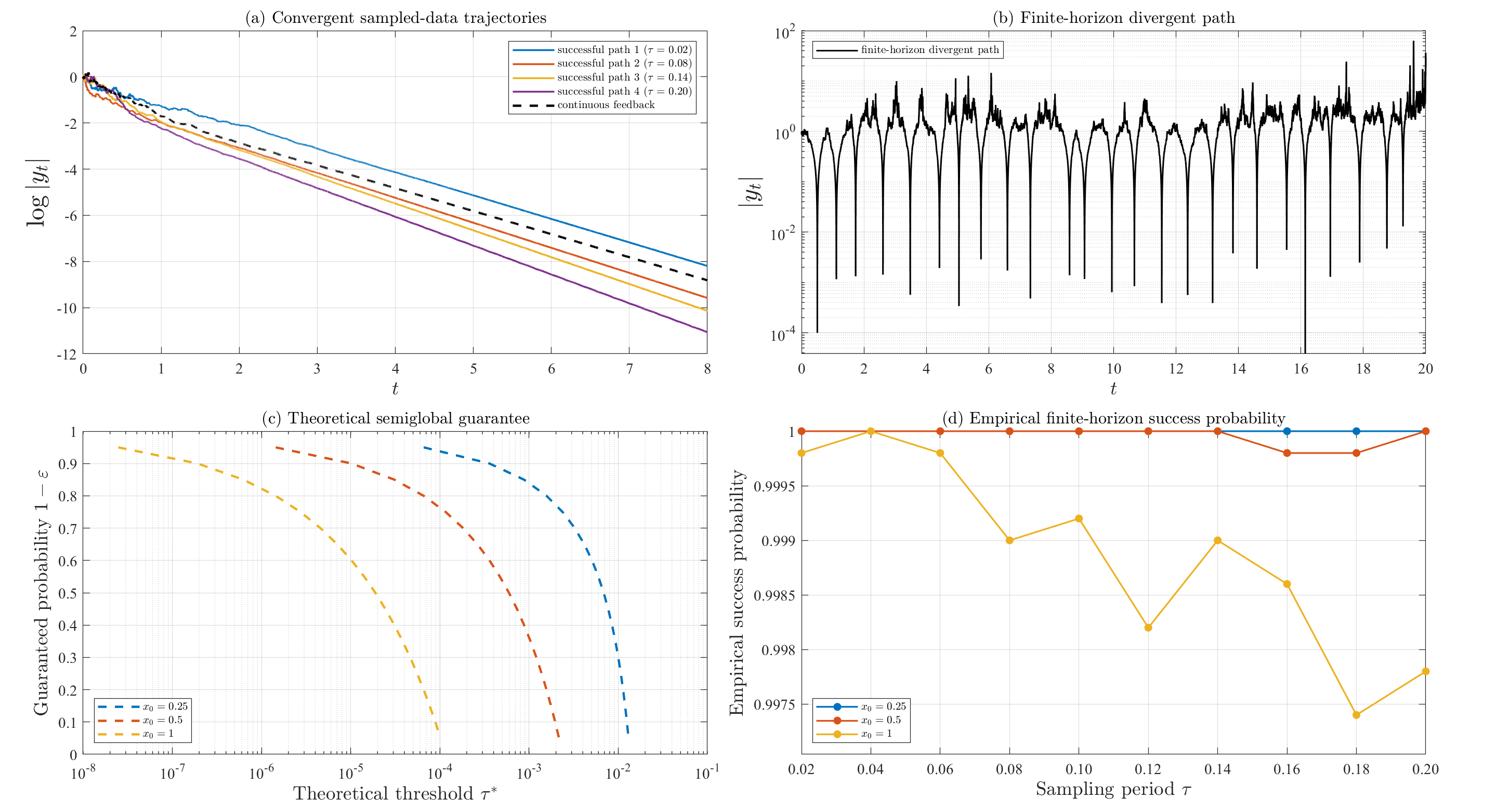
Eq. (51) does not explode in finite time, but numerical evidence shows that some sample paths are oscillatory and unbounded above, with $\limsup_{t\to\infty}|y_{t}|=\infty$ and $\liminf_{t\to\infty}|y_{t}|=0$ , which precisely verifies the conclusion of Lemma 28.

Figure 2(a) shows representative convergent paths with exponential decay after a short transient. Panel (b) displays a divergent sample path that remains finite over the simulated time horizon but oscillates between near-zero values and arbitrarily large amplitudes, and hence does not converge to the origin. Panel (c) plots the theoretical sufficient threshold $\tau_{2}^{*}(x_{0},\varepsilon)$ , computed from Theorem 14. Panel (d) shows the finite-horizon empirical success probabilities from $5000$ Monte Carlo simulations, which remain close to one over the tested range. As in Example 1, the gap between panels (c) and (d) illustrates the conservativeness of the sufficient theoretical bounds.

6 Concluding Remarks

This paper studies sampled-data stabilization of nonlinear stochastic systems under a local exponential-type Lyapunov condition on the continuous-time closed-loop system, with only locally Lipschitz coefficients and without imposing linear growth or Khasminskii-type conditions. Two counterexamples show that almost sure stability is generally not attainable. Instead, for any initial state, we prove exponential stability with arbitrarily high probability under sufficiently fast sampling. The cases $p\geq 2$ and $0<p<2$ are treated using a generalized Halanay inequality and a comparison method, respectively. Future work includes deriving sharper sampling bounds and extending the results to broader control frameworks.

7 Appendix

7.1 Appendix A

In this subsection, we give a proof of Lemma 10.

Proof of Lemma 10.

Define $F(\mu)\triangleq\mu-a+b{\mathrm{e}}^{\mu\tau}$ . Since $a>b$ , $F(0)=b-a<0$ . Moreover, $F^{\prime}(\mu)=1+b\tau{\mathrm{e}}^{\mu\tau}>0,$ and $F(\mu)\to\infty$ as $\mu\to\infty$ . Hence there is a unique $\mu>0$ such that $F(\mu)=0$ , which is exactly $\mu=a-b{\mathrm{e}}^{\mu\tau}$ .

Set $C\triangleq\sup_{-\tau\leq s\leq 0}\Phi(s)$ and define the comparison function $W(t)\triangleq C{\mathrm{e}}^{-\mu t},\ \ t\geq-\tau.$ Since $W$ is nonincreasing, $\sup_{-\tau\leq\theta\leq 0}W(t+\theta)=W(t-\tau)={\mathrm{e}}^{\mu\tau}W(t).$ Using $\mu=a-b{\mathrm{e}}^{\mu\tau}$ , we obtain

W^{\prime}(t)=-aW(t)+b\sup_{-\tau\leq\theta\leq 0}W(t+\theta),\hskip 9.24994ptt\geq 0.

(52)

We now prove that $\Phi(t)\leq W(t)$ for all $t\geq 0$ . Fix $\epsilon>0$ and set $A_{\epsilon}\triangleq\{t\geq 0:\ \Phi(t)>W(t)+\epsilon\}.$ Suppose, for contradiction, that $A_{\epsilon}\neq\varnothing$ , and let $t_{*}\triangleq\inf A_{\epsilon}.$ For every $t\in[-\tau,0]$ , the definition of $C$ gives $\Phi(t)\leq C\leq C{\mathrm{e}}^{-\mu t}=W(t)<W(t)+\epsilon.$ By the definition of $t_{*}$ , we also have $\Phi(t)\leq W(t)+\epsilon$ for $0\leq t<t_{*}$ . By the continuity of $W$ , $\liminf_{t\to t_{*}^{-}}\Phi(t)\leq W(t_{*})+\epsilon.$ By the second inequality in (11), $\Phi(t_{*})\leq\liminf_{t\to t_{*}^{-}}\Phi(t),$ and hence

\Phi(t_{*})\leq W(t_{*})+\epsilon.

(53)

Thus $t_{*}\notin A_{\epsilon}$ . Since $t_{*}=\inf A_{\epsilon}$ , there exists a sequence $t_{n}\in A_{\epsilon}$ such that $t_{n}\downarrow t_{*}$ . Hence $\Phi(t_{n})>W(t_{n})+\epsilon.$ It follows that $\limsup_{t\to t_{*}^{+}}\Phi(t)\geq\limsup_{n\to\infty}\Phi(t_{n})\geq W(t_{*})+\epsilon.$ By the first inequality in (11), $\limsup_{t\to t_{*}^{+}}\Phi(t)\leq\Phi(t_{*}),$ so

\Phi(t_{*})\geq W(t_{*})+\epsilon.

(54)

Combining (53) and (54), we obtain

\Phi(t_{*})=W(t_{*})+\epsilon.

(55)

By the definition of the upper right Dini derivative and by (55),

		$\displaystyle D^{+}\Phi(t_{})\geq\limsup_{n\to\infty}\frac{\Phi(t_{n})-\Phi(t_{})}{t_{n}-t_{}}\geq\limsup_{n\to\infty}\frac{W(t_{n})-W(t_{})}{t_{n}-t_{}}=W^{\prime}(t_{})$		(56)
		$\displaystyle=-aW(t_{})+b\sup_{-\tau\leq\theta\leq 0}W(t_{}+\theta)\geq-a\bigl(\Phi(t_{})-\epsilon\bigr)+b\left(\sup_{-\tau\leq\theta\leq 0}\Phi(t_{}+\theta)-\epsilon\right)$
		$\displaystyle=-a\Phi(t_{})+b\sup_{-\tau\leq\theta\leq 0}\Phi(t_{}+\theta)+(a-b)\epsilon,$

which contradicts (12). Therefore $A_{\epsilon}=\varnothing$ . Letting $\epsilon\to 0$ yields the result.

Remark 25.

Condition (11) allows discontinuities but rules out upward jumps: every right-hand cluster value is no larger than $\Phi(t)$ , while every left-hand cluster value is no smaller than $\Phi(t)$ . These are precisely the one-sided regularity properties used in the first-crossing argument.

7.2 Appendix B

We prove the claims of the two examples in the Introduction. Given any nonzero initial value and any $\tau>0$ , almost sure stability fails. The proof relies on the support theorem (Theorem 26; see also [26, (5.1)–(5.2)]), which states that for an SDE in Stratonovich form, its solutions approximate those of the associated deterministic ODE with positive probability (cf. [11, Theorem 3.3]).

Theorem 26 (Support theorem).

Let $X_{0}(t,x)$ be a bounded measurable function, uniformly Lipschitz continuous in $x$ , and let $X_{k}(t,x)$ , $k=1,\ldots,n$ , be continuously differentiable in $t$ and twice continuously differentiable in $x$ , with bounded derivatives. Consider the Stratonovich equation

\mathrm{d}x_{t}=X_{0}(t,x_{t})\,\mathrm{d}t+\sum_{k=1}^{n}X_{k}(t,x_{t})\circ\mathrm{d}W_{t}^{k},\hskip 9.24994ptx_{0}=x.

Let $\mathbb{P}_{x}$ be the probability law of the solution $x_{t}$ starting at $x$ . Consider, in addition, the associated deterministic control system

\frac{\mathrm{d}}{\mathrm{d}t}x_{v}(t)=X_{0}(t,x_{v}(t))+\sum_{k=1}^{n}X_{k}(t,x_{v}(t))v^{k}(t),\hskip 9.24994ptx_{v}(0)=x,

with $v^{k}\in\mathcal{V}$ , where $\mathcal{V}$ is the set of all piecewise constant functions from $\mathbb{R}_{+}$ to $\mathbb{R}$ .

Let $\mathcal{W}_{x}$ be the set of all continuous paths from $\mathbb{R}_{+}$ to $\mathbb{R}$ starting at $x$ , equipped with the topology of uniform convergence on compact sets, and let $\mathcal{I}_{x}$ be the smallest closed subset of $\mathcal{W}_{x}$ such that $\mathbb{P}_{x}(x_{\cdot}\in\mathcal{I}_{x})=1$ . Then

\mathcal{I}_{x}=\overline{\{x_{v}(\cdot)\in\mathcal{W}_{x}:\ v\in\mathcal{V}^{n}\}}\subset\mathcal{W}_{x}.

The preceding theorem immediately implies the following fact. If $x_{v}(\cdot)$ is a controlled trajectory generated by some $v\in\mathcal{V}^{n}$ , then $x_{v}(\cdot)\in\mathcal{I}_{x}$ . Hence, for every $T>0$ and every $\eta>0$ , $\mathbb{P}_{x}\left(\sup_{0\leq t\leq T}|x_{t}-x_{v}(t)|<\eta\right)>0$ .

Lemma 27.

Consider the $1$ -dimensional stochastic system

\mathrm{d}x_{t}=\left(x_{t}^{2}+x_{t}^{3}-C\right)\,\mathrm{d}t+x_{t}^{2}\,\mathrm{d}B_{t},\hskip 9.24994ptx_{0}>0.

(57)

Here, $C$ is a constant. Let the stopping time $\sigma_{N}\triangleq\inf\{t\geq 0:\ |x_{t}|\geq N\},$ and let $\sigma_{\infty}\triangleq\lim_{N\rightarrow+\infty}\sigma_{N}$ denote the explosion time of the maximal local solution. Then for any $\tau>0$ , $\mathbb{P}(\sigma_{\infty}<\tau)>0.$ This implies that system (3) with a sampled-data control will explode in any arbitrarily short time with positive probability.

Proof.

Let $y_{t}=\displaystyle\frac{1}{x_{t}}$ . Then $y_{t}$ satisfies the following SDE on the interval $[0,\sigma_{\infty}\wedge\theta_{0})$ :

{\mathrm{d}}y_{t}=(-1+Cy_{t}^{2})\,{\mathrm{d}}t-{\mathrm{d}}B_{t},\hskip 9.24994pty_{0}=\displaystyle\frac{1}{x_{0}},

(58)

where $\theta_{0}\triangleq\inf\{t\geq 0:|x_{t}|=0\}$ . Choose $f\in C_{b}^{\infty}(\mathbb{R})$ such that $f(r)=-1+Cr^{2}$ for $r\in[-2,\displaystyle\frac{1}{x_{0}}+1]$ . We consider the auxiliary process

\mathrm{d}z_{t}=f(z_{t})\,\mathrm{d}t-\mathrm{d}B_{t},\hskip 9.24994ptz_{0}=\frac{1}{x_{0}}>0.

(59)

In the following, we use Theorem 26 to prove that the solution $z_{t}$ of Eq. (59) satisfies $\mathbb{P}(\kappa_{0}<\tau\wedge\kappa_{1})>0$ , where $\kappa_{0}\triangleq\inf\{t>0:z_{t}=0\},\kappa_{1}\triangleq\inf\{t>0:z_{t}=\frac{1}{x_{0}}+\frac{1}{2}\}$ . This suffices to show that $\mathbb{P}(\sigma_{\infty}<\tau)>0$ since $y_{t}=z_{t}$ on the interval $[0,\kappa_{0}\wedge\kappa_{1})$ .

By Theorem 26, we consider the associated deterministic control system

\dot{r}(t)=f(r(t))-v(t),\hskip 9.24994ptr(0)=\displaystyle\frac{1}{x_{0}}.

(60)

Choose a constant control function $v(t)\equiv M$ , where $M>\sup_{r\in\mathbb{R}}|f(r)|+\frac{2(z_{0}+1)}{\tau}.$ Then the corresponding controlled trajectory of Eq. (60) satisfies $\dot{r}(t)\leq\sup_{r\in\mathbb{R}}|f(r)|-M<-\frac{2(z_{0}+1)}{\tau}.$ Set $t_{1}\triangleq\inf\{t\geq 0:\ r(t)=-1\}$ . It is easy to verify that $t_{1}<\frac{\tau}{2}$ , and $r(t)$ is monotonically decreasing on $[0,t_{1}]$ while $r(t_{1})=-1$ . By Theorem 26, we have $\mathbb{P}\left(\sup_{0\leq t\leq t_{1}}|z_{t}-r(t)|<\frac{1}{2}\right)>0.$ Since $r(t)\in[-1,z_{0}]$ for $t\in[0,t_{1}]$ and $r(t_{1})=-1$ . Then on the event $A\triangleq\left\{\sup_{0\leq t\leq t_{1}}|z_{t}-r(t)|<\frac{1}{2}\right\}$ , we have $z_{t}\in(-\frac{3}{2},z_{0}+\frac{1}{2})$ and $z_{t_{1}}<-\frac{1}{2}$ . Thus, we know $A\subseteq\{\kappa_{0}<\tau\wedge\kappa_{1}\}$ and consequently $\mathbb{P}(\{\kappa_{0}<\tau\wedge\kappa_{1}\})\geq\mathbb{P}(A)>0$ .

Lemma 28.

Consider the stochastic hybrid system $(\kappa>1)$

\mathrm{d}x_{t}=\left[x_{t}-\kappa x_{t_{n}}-x_{t_{n}}^{3}\right]\mathrm{d}t+x_{t}^{2}\,\mathrm{d}B_{t},\hskip 9.24994ptt\in[t_{n},t_{n+1}],

(61)

with initial value $x_{0}\neq 0$ and sampling instants $t_{n}=n\tau$ . Then, for every $\tau>0$ , the solution exists for all $t\geq 0$ , and moreover

{\color[rgb]{0,0,0}\mathbb{P}\left(\lim_{n\to+\infty}|x_{t_{n}}|=+\infty,\ \liminf_{t\to+\infty}|x_{t}|=0\right)>0.}

Proof.

On each sampling interval, Eq. (61) can be written as ${\rm d}x_{t}=(x_{t}+C){\rm d}t+x_{t}^{2}{\rm d}B_{t}$ . Thus, for $\Phi(x)=\log(1+x^{2})$ , $\mathcal{L}\Phi(x)\to-\infty$ as $|x|\to+\infty$ . Therefore, $\mathcal{L}\Phi(x)$ is bounded above, and hence the solution exists on each interval. By induction, the solution exists globally. The proof of the remaining part is divided into three steps.

Step 1: On the first sampling interval $[0,\tau]$ , we prove $\mathbb{P}(|x_{\tau}|>R)>0$ for large $R>0$ . To this end, we rewrite (61) in the Stratonovich form on $[0,\tau]$ :

{\mathrm{d}}x_{t}=(x_{t}-{x_{t}^{3}}-C){\mathrm{d}}t+x_{t}^{2}\circ\mathrm{d}B_{t},

where $C\triangleq\kappa x_{0}+x_{0}^{3}\neq 0$ . Consider the associated deterministic control system

\dot{r}(t)=r(t)-r(t)^{3}-C+r(t)^{2}v(t),\hskip 9.24994ptr(0)=x_{0}.

By choosing a constant control $v(t)\equiv M$ (or $-M$ ) sufficiently large, we have $|r(\tau)|>R$ . Following a similar argument to the proof of Lemma 27, the Support Theorem 26 guarantees that $\mathbb{P}(|x_{\tau}|>R)>0$ .

Step 2: We prove that there exist $R>0$ and $\theta,q\in(0,1)$ such that on $[0,\tau]$ ,

|x_{0}|\geq R\hskip 9.24994pt\Longrightarrow\hskip 9.24994pt\mathbb{E}(1+|x_{\tau}|)^{-\theta}\leq q(1+|x_{0}|)^{-\theta}.

(62)

Set $r=|x_{0}|,x_{t}=x_{0}Z_{s},s=r^{2}t,\widetilde{B}_{s}=x_{0}B_{s/r^{2}}.$ Then (61) on $[0,\tau]$ becomes

\mathrm{d}Z_{s}=f_{r}(Z_{s})\,\mathrm{d}s+Z_{s}^{2}\,\mathrm{d}\widetilde{B}_{s},

(63)

with initial value $Z_{0}=1$ , where $f_{r}(z)\triangleq-1+\frac{z-\kappa}{r^{2}}$ , $\widetilde{B}_{s}$ is a standard Brownian motion. The interval $(-\infty,0)$ is invariant under (63). Moreover, (63) admits an invariant probability measure $\mu_{r}$ on $(-\infty,0)$ , whose density $\pi_{r}$ satisfies the stationary Fokker–Planck equation $-\frac{\mathrm{d}}{\mathrm{d}z}\bigl(f_{r}(z)\pi_{r}(z)\bigr)+\frac{1}{2}\frac{\mathrm{d}^{2}}{\mathrm{d}z^{2}}\bigl(z^{4}\pi_{r}(z)\bigr)=0$ for $z<0$ . Its normalized zero-flux solution is $\pi_{r}(z)\triangleq C_{r}|z|^{-4}\exp\left\{-\frac{1}{r^{2}z^{2}}+\frac{2}{3z^{3}}\left(1+\frac{\kappa}{r^{2}}\right)\right\}\mathbf{1}_{z<0}$ where $C_{r}>0$ is the normalizing constant. In what follows, we show that the solution of (63) rapidly enters $(-\infty,0)$ and then use synchronous coupling to establish its rapid convergence to the invariant distribution. This will yield (62). Indeed, (62) is equivalent to

\left(1+\frac{1}{r}\right)^{\theta}\mathbb{E}\left[\left(|Z_{r^{2}\tau}|+\frac{1}{r}\right)^{-\theta}\right]\leq q.

(64)

Define the stopping times $\zeta\triangleq\inf\{s\geq 0:Z_{s}=-1\}$ . Then

		$\displaystyle\mathbb{E}\left[\left(\|Z_{r^{2}\tau}\|+\frac{1}{r}\right)^{-\theta}\right]=\mathbb{E}\left[\left(\|Z_{r^{2}\tau}\|+\frac{1}{r}\right)^{-\theta};\zeta>\frac{r^{2}\tau}{2}\right]+\mathbb{E}\left[\left(\|Z_{r^{2}\tau}\|+\frac{1}{r}\right)^{-\theta};\zeta\leq\frac{r^{2}\tau}{2}\right]$
	$\displaystyle\leq{}$	$\displaystyle\underbrace{r^{\theta}\mathbb{P}\left(\zeta>\frac{r^{2}\tau}{2}\right)}_{I_{1}}+\underbrace{\mathbb{E}\left[\mathbf{1}_{\{\zeta\leq r^{2}\tau/2\}}\mathbb{E}\left[\left.\left(\|Z_{r^{2}\tau}\|+\frac{1}{r}\right)^{-\theta}\,\right\|\,\mathscr{F}_{\zeta}\right]\right]}_{I_{2}}.$

As to estimate $I_{1}$ , denote by $H(x)=2-\frac{1}{(x+2)^{2}}$ , then $1\leq H(x)<2$ for $x\geq-1$ . We compute that $\mathcal{L}_{r}H(x)=-\frac{2(x+2)+3x^{4}}{(x+2)^{4}}+\frac{2(x-\kappa)}{r^{2}(x+2)^{3}}\leq-A+B/r^{2}$ , where $A\triangleq\inf_{x\geq-1}\frac{2(x+2)+3x^{4}}{(x+2)^{4}}>0$ , $B\triangleq\sup_{x\geq-1}\frac{2(x-\kappa)}{(x+2)^{3}}<+\infty$ . When $r\geq\sqrt{\frac{2B}{A}}$ , we have $\mathcal{L}_{r}H(x)\leq-\frac{A}{2}\leq-\lambda_{1}H(x)$ , where $\lambda_{1}\triangleq\frac{A}{4}$ . Consequently, we have $2>H(Z_{0})\geq\mathbb{E}[{\rm e}^{\lambda_{1}(t\wedge\zeta)}H(Z_{t\wedge\zeta})]\geq{\rm e}^{\lambda_{1}t}\mathbb{P}(\zeta>t).$ This yields that $I_{1}\leq 2r^{\theta}{\rm e}^{-\lambda_{1}r^{2}\tau/2}$ .

To estimate $I_{2}$ , consider (63) with $Z_{0}=-1$ and set $Y_{s}=-1/Z_{s}$ . Itô’s formula gives $\mathrm{d}Y_{s}=b_{r}(Y_{s})\,\mathrm{d}s+\mathrm{d}\widetilde{B}_{s},Y_{0}=1,$ where $b_{r}(y)\triangleq\frac{1}{y}-\left(1+\frac{\kappa}{r^{2}}\right)y^{2}-\frac{y}{r^{2}}$ . A direct calculation gives $b_{r}^{\prime}(y)=-\frac{1}{y^{2}}-2\left(1+\frac{\kappa}{r^{2}}\right)y-\frac{1}{r^{2}}\leq-\frac{1}{y^{2}}-2y\leq-3$ . Let $\overline{Z}_{0}$ be independent of $\widetilde{B}$ and have density $\pi_{r}$ , and set $\overline{Y}_{0}=-1/\overline{Z}_{0}$ . Consider the auxiliary process $\mathrm{d}\overline{Y}_{s}=b_{r}(\overline{Y}_{s})\,\mathrm{d}s+\mathrm{d}\widetilde{B}_{s},$ driven by the same Brownian motion as $Y_{s}$ . Since $b_{r}^{\prime}(y)\leq-3$ , $\mathbb{E}|Y_{s}-\overline{Y}_{s}|^{2}\leq\mathrm{e}^{-6s}\mathbb{E}|Y_{0}-\overline{Y}_{0}|^{2}=\mathrm{e}^{-6s}\mathbb{E}|1-\overline{Y}_{0}|^{2}.$ Using $|Z_{s}|=1/Y_{s}$ , $\theta\in(0,1)$ , $\overline{Y}_{s}$ has the same distribution as $\overline{Y}_{0}$ , we have

		$\displaystyle\mathbb{E}\left[\left(\|Z_{s}\|+\frac{1}{r}\right)^{-\theta}\right]=\mathbb{E}\left[\left(\frac{1}{Y_{s}}+\frac{1}{r}\right)^{-\theta}\right]\leq\mathbb{E}\left\|\left(\frac{rY_{s}}{r+Y_{s}}\right)^{\theta}-\left(\frac{r\overline{Y}_{s}}{r+\overline{Y}_{s}}\right)^{\theta}\right\|+\mathbb{E}\left(\frac{r\overline{Y}_{s}}{r+\overline{Y}_{s}}\right)^{\theta}$
		$\displaystyle\leq\mathbb{E}\left\|\frac{rY_{s}}{r+Y_{s}}-\frac{r\overline{Y}_{s}}{r+\overline{Y}_{s}}\right\|^{\theta}+\mathbb{E}\left(\frac{r\overline{Y}_{s}}{r+\overline{Y}_{s}}\right)^{\theta}\leq\mathbb{E}\|Y_{s}-\overline{Y}_{s}\|^{\theta}+\mathbb{E}\left(\frac{r\overline{Y}_{s}}{r+\overline{Y}_{s}}\right)^{\theta}$
		$\displaystyle\leq\mathrm{e}^{-3\theta s}\left(\mathbb{E}\|1-\overline{Y}_{0}\|^{2}\right)^{\theta/2}+\mathbb{E}\left(\frac{r\overline{Y}_{0}}{r+\overline{Y}_{0}}\right)^{\theta}\leq C_{1}{\rm e}^{-3\theta s}+\mathbb{E}\left(\frac{r\overline{Y}_{0}}{r+\overline{Y}_{0}}\right)^{\theta}$
		$\displaystyle=C_{1}{\rm e}^{-3\theta s}+\mathbb{E}\left(\|\overline{Z}_{0}\|+\frac{1}{r}\right)^{-\theta}=C_{1}{\rm e}^{-3\theta s}+\int_{-\infty}^{0}\left(\|z\|+\frac{1}{r}\right)^{-\theta}\pi_{r}(z)\mathrm{d}z.$

Choosing $\theta=1/2$ , letting $r\to+\infty$ , the second term is approximated as

\displaystyle\lim_{r\to\infty}\mathbb{E}\left(\frac{r\overline{Y}_{0}}{r+\overline{Y}_{0}}\right)^{\theta}

\displaystyle=2\int_{-\infty}^{0}|z|^{-\theta-4}\exp\left(\frac{2}{3z^{3}}\right)\mathrm{d}z=\left(\frac{3}{2}\right)^{\theta/3}\Gamma\left(1+\frac{\theta}{3}\right)\approx 0.9926<1.

Therefore, there exist $q_{0}\in(0.9926,1)$ and $R_{0}$ such that for $r\geq R_{0}$ , $\mathbb{E}\left(\frac{r\overline{Y}_{0}}{r+\overline{Y}_{0}}\right)^{1/2}\leq q_{0}.$ By strong Markov property, $I_{2}\leq C_{1}\mathrm{e}^{-3\theta r^{2}\tau/2}+q_{0}$ . Combining this with the estimate of $I_{1}$ , we obtain $I_{1}+I_{2}\leq 2r^{\theta}\mathrm{e}^{-\lambda_{1}r^{2}\tau/2}+C_{1}\mathrm{e}^{-3\theta r^{2}\tau/2}+q_{0}.$ Choosing $q\in(q_{0},1)$ and then $R\geq R_{0}$ sufficiently large ensures that (64) holds for every $r\geq R$ .

Step 3: Denote by $X_{n}\triangleq x_{n\tau}$ , $\mathscr{G}_{n}\triangleq\mathscr{F}_{n\tau}$ . Shifting (62) to $[n\tau,(n+1)\tau]$ yields

\mathbb{E}[W(X_{n+1})\cdot\mathbf{1}_{|X_{n}|\geq R}\mid\mathscr{G}_{n}]\leq qW(X_{n})\cdot\mathbf{1}_{|X_{n}|\geq R},

(65)

where $W(x)\triangleq(1+|x|)^{-\theta}$ . We first suppose $|X_{1}|\geq 2R$ as a deterministic value, denote by $\eta\triangleq\inf\{n\in\mathbb{N}\mid|X_{n}|<R\}$ . By $\{\eta\geq n+1\}\subseteq\{|X_{n}|\geq R\}$ ,

\mathbb{E}[W(X_{(n+1)\wedge\eta})-W(X_{n\wedge\eta})\mid\mathscr{G}_{n}]=\mathbb{E}[W(X_{n+1})-W(X_{n})\mid\mathscr{G}_{n}]\cdot\mathbf{1}_{\eta\geq n+1}\leq 0.

Taking expectation yields that

\mathbb{E}W(X_{(n+1)\wedge\eta})\leq\mathbb{E}W(X_{n\wedge\eta})\leq\cdots\leq W(X_{1})\leq W(2R).

Consequently, we obtain $W(2R)\geq\mathbb{E}W(X_{(n+1)\wedge\eta})\geq\mathbb{E}[W(X_{\eta});\eta\leq n+1]\geq W(R)\mathbb{P}(\eta\leq n+1).$ Letting $n\to+\infty$ yields that $\mathbb{P}(\eta<+\infty)\leq W(2R)/W(R)$ . Thus we have $\mathbb{P}(\eta=+\infty)\geq 1-W(2R)/W(R)>0.$ Multiplying $\mathbf{1}_{\eta\geq n+1}$ on both sides of (65) and taking expectations yields that

\mathbb{E}[W(X_{n+1})\mathbf{1}_{\eta\geq n+2}]\leq\mathbb{E}[W(X_{n+1})\mathbf{1}_{\eta\geq n+1}]\leq q\mathbb{E}[W(X_{n})\mathbf{1}_{\eta\geq n+1}]\leq\cdots\leq q^{n}W(X_{1}).

Thus,

\sum_{n=1}^{+\infty}\mathbb{P}(W(X_{n+1})\geq q^{(1-\epsilon)n};\eta\geq n+2)\leq\sum_{n=1}^{+\infty}q^{\epsilon n}W(X_{1})<+\infty.

By the Borel Cantelli Lemma, $\liminf_{n\to+\infty}\frac{\log|X_{n}|}{n}\geq-\frac{1-\epsilon}{\theta}\log q>0\hskip 9.24994pt\text{a.s. on }\{\eta=\infty\}.$

On the other hand, the preceding estimate gives $\mathbb{P}\left(\inf_{t\in[0,\tau]}|x_{t}|>0\right)\leq\mathbb{P}(\zeta>r^{2}\tau)\leq 2\mathrm{e}^{-\lambda_{1}|x_{0}|^{2}\tau}.$ Shifting this estimate to each sampling interval $[t_{n},t_{n+1}]$ and using the preceding exponential-growth result, we obtain

\sum_{n=1}^{\infty}\mathbb{P}\left(\left.\inf_{t\in[t_{n},t_{n+1}]}|x_{t}|>0,\,\eta\geq n+1\,\right|\,\mathscr{G}_{n}\right)\leq\sum_{n=1}^{\infty}2\mathrm{e}^{-\lambda_{1}|X_{n}|^{2}\tau}\mathbf{1}_{\{\eta\geq n+1\}}<\infty\hskip 9.24994pt\text{a.s.}.

Hence, by the conditional Borel–Cantelli lemma, $\liminf_{t\to\infty}|x_{t}|=0\hskip 9.24994pt\text{a.s. on }\{\eta=\infty\}.$

Finally, we return to the proof of Lemma 28. By Step 1, $\mathbb{P}(\mathcal{A})>0(\mathcal{A}\triangleq\{|X_{1}|>2R\}).$ Thus

\mathbb{P}(\limsup_{n\to+\infty}|x_{t_{n}}|=+\infty,\liminf_{t\to\infty}|x_{t}|=0)\geq\mathbb{P}(\eta=+\infty;\mathcal{A})=\mathbb{P}(\eta=+\infty\mid\mathcal{A})\mathbb{P}(\mathcal{A})>0.

This completes the proof.

References

[1] C. T.H. Baker and E. Buckwar (2005) Exponential stability in p-th mean of solutions, and of convergent euler-type solutions, of stochastic delay differential equations. J. Comput. Appl. Math. 184 (2), pp. 404–427. External Links: ISSN 0377-0427 Cited by: §3.1.
[2] J. C. Dias, J. P. V. Nunes, and A. Cruz (2020) A note on options and bubbles under the cev model: implications for pricing and hedging: jc dias et al.. Review of Derivatives Research 23 (3), pp. 249–272. Cited by: Example 2.
[3] H. Dong, J. Tang, and X. Mao (2022) Stabilization of highly nonlinear hybrid stochastic differential delay equations with lévy noise by delay feedback control. SIAM J. Control Optim. 60 (6), pp. 3302–3325. Cited by: 1st item, §1.
[4] C. Fei, W. Fei, X. Mao, D. Xia, and L. Yan (2020) Stabilization of highly nonlinear hybrid systems by feedback control based on discrete-time state observations. IEEE Trans. Automat. Control 65 (7), pp. 2899–2912. Cited by: 1st item, §1.
[5] J. Hu, W. Liu, F. Deng, and X. Mao (2020) Advances in stabilization of hybrid stochastic differential equations by delay feedback control. SIAM J. Control Optim. 58 (2), pp. 735–754. Cited by: §1.
[6] K. Ide and D. Sornette (2002) Oscillatory finite-time singularities in finance, population and rupture. Physica A: Statistical Mechanics and its Applications 307 (1-2), pp. 63–106. Cited by: Example 1.
[7] F. Li and Y. Liu (2020) Event-triggered stabilization for continuous-time stochastic systems. IEEE Trans. Automat. Control 65 (10), pp. 4031–4046. Cited by: §1.
[8] F. Li and Y. Liu (2021) An enlarged framework of event-triggered control for stochastic systems. IEEE Trans. Automat. Control 66 (9), pp. 4132–4147. Cited by: §1.
[9] X. Li, X. Mao, D. S. Mukama, and C. Yuan (2020) Delay feedback control for switching diffusion systems based on discrete-time observations. SIAM J. Control Optim. 58 (5), pp. 2900–2926. Cited by: §1.
[10] X. Li and X. Mao (2020) Stabilisation of highly nonlinear hybrid stochastic differential delay equations by delay feedback control. Automatica 112, pp. 108657. External Links: ISSN 0005-1098 Cited by: 1st item, §1.
[11] W. Liang, N. H. Amini, and P. Mason (2019) On exponential stabilization of $n$-level quantum angular momentum systems. SIAM J. Control Optim. 57 (6), pp. 3939–3960. Cited by: §7.2.
[12] W. Lin (2020) When is a nonlinear system semiglobally asymptotically stabilizable by digital feedback?. IEEE Trans. Automat. Control 65 (11), pp. 4584–4599. Cited by: §1, §1, §1, §1, §1, §1, Remark 6.
[13] K. Liu, A. R. Teel, and X. Sun (2022) Event-triggered nonlinear systems with stochastic dynamics, transmission times, and protocols. IEEE Trans. Automat. Control 67 (4), pp. 1973–1979. Cited by: §1.
[14] K. Liu, A. R. Teel, and X. Sun (2024) A stochastic hybrid framework for event-triggered nonlinear control systems with stochastic denial of service attacks. IEEE Trans. Automat. Control 69 (2), pp. 904–919. Cited by: §1.
[15] W. Liu, W. Mao, X. Mao, and J. Zhou (2025) Stabilization of hybrid systems by event-triggered control based on discrete-time state observations. SIAM J. Control Optim. 63 (5), pp. 3501–3525. Cited by: §1.
[16] X. Mao, J. Lam, and L. Huang (2008) Stabilisation of hybrid stochastic differential equations by delay feedback control. Systems Control Lett. 57 (11), pp. 927–935. External Links: ISSN 0167-6911 Cited by: §1.
[17] X. Mao, W. Liu, L. Hu, Q. Luo, and J. Lu (2014) Stabilization of hybrid stochastic differential equations by feedback control based on discrete-time state observations. Systems Control Lett. 73, pp. 88–95. External Links: ISSN 0167-6911 Cited by: §1.
[18] X. Mao (1999) LaSalle-type theorems for stochastic differential delay equations. J. Math. Anal. Appl. 236 (2), pp. 350–369. Cited by: Remark 6.
[19] X. Mao (1999) Stochastic versions of the lasalle theorem. J. Differential Equations 153 (1), pp. 175–195. Cited by: Remark 6.
[20] X. Mao (2007) Stochastic differential equations and applications. Elsevier. Cited by: §3.1, §4.2, Remark 6, Remark 7.
[21] X. Mao (2013) Stabilization of continuous-time hybrid stochastic differential equations by discrete-time feedback control. Automatica 49 (12), pp. 3677–3681. External Links: ISSN 0005-1098 Cited by: 1st item, 3rd item, §1, §1, §4.
[22] X. Mao (2015) Almost sure exponential stabilization by discrete-time stochastic feedback control. IEEE Trans. Automat. Control 61 (6), pp. 1619–1624. Cited by: 1st item, 3rd item, §1, §1, §4.
[23] C. Mei, C. Fei, W. Fei, and X. Mao (2020) Stabilisation of highly non-linear continuous-time hybrid stochastic differential delay equations by discrete-time feedback control. IET Control Theory Appl. 14 (2), pp. 313–323. Cited by: 1st item, §1.
[24] Q. Qiu, W. Liu, L. Hu, X. Mao, and S. You (2016) Stabilization of stochastic differential equations with markovian switching by feedback control based on discrete-time state observation with a time delay. Statist. Probab. Lett. 115, pp. 16–26. External Links: ISSN 0167-7152 Cited by: §1.
[25] H. Shim and A. R. Teel (2003) Asymptotic controllability and observability imply semiglobal practical asymptotic stabilizability by sampled-data output feedback. Automatica 39 (3), pp. 441–454. Cited by: Remark 6.
[26] D. W. Stroock and S. R. S. Varadhan (1972) On the support of diffusion processes with applications to the strong maximum principle. In Proceedings of the Sixth Berkeley Symposium on Mathematical Statistics and Probability, Vol. 3, Berkeley, California, pp. 333–359. Note: University of California, Berkeley, California, 1970/1971 Cited by: §7.2.
[27] H. Xu, X. Mao, and G. Yin (2026) Stability and stabilization using discrete-time feedback control for hybrid stochastic delay systems with general delay. SIAM J. Control Optim. 64 (4), pp. 2844–2869. Cited by: 2nd item, §1, §3.1.
[28] H. Xu and X. Mao (2023) Advances in discrete-state-feedback stabilization of highly nonlinear hybrid systems by razumikhin technique. IEEE Trans. Automat. Control 68 (10), pp. 6098–6113. Cited by: 1st item, §1.
[29] X. Yang, Q. Zhu, and H. Wang (2024) Exponential stabilization of stochastic systems via novel event-triggered switching controls. IEEE Trans. Automat. Control 69 (11), pp. 7948–7955. Cited by: §1.
[30] S. You, W. Liu, J. Lu, X. Mao, and Q. Qiu (2015) Stabilization of hybrid systems by feedback control based on discrete-time state observations. SIAM J. Control Optim. 53 (2), pp. 905–925. Cited by: §1.
[31] X. Yu and W. Lin (2024) On input delay tolerance of stochastic nonlinear systems with dominant homogeneity of degree zero. IEEE Trans. Automat. Control 69 (10), pp. 6935–6950. Cited by: §1, §1.
[32] X. Yu and W. Lin (2024) Sampled-data feedback stabilization in mean square for stochastic homogeneous systems. IEEE Trans. Automat. Control 69 (10), pp. 6805–6820. Cited by: §1.
[33] X. Yu and W. Lin (2025) Almost sure asymptotic stabilization of stochastic nonlinear systems by sampled-data state and output feedback. IEEE Trans. Automat. Control 70 (2), pp. 1131–1146. Cited by: §1.
[34] Q. Zhu (2024) Event-triggered sampling problem for exponential stability of stochastic nonlinear delay systems driven by lévy processes. IEEE Trans. Automat. Control 70 (2), pp. 1176–1183. Cited by: §1.

		$\displaystyle\\|\bm{f}(\bm{x},\bm{\alpha}(\bm{z}))\\|^{p}\leq M_{f,R}^{(p)}\left(\\|\bm{x}\\|^{p}+\\|\bm{z}\\|^{p}\right),\\|\bm{g}(\bm{x},\bm{\alpha}(\bm{z}))\\|^{p}\leq M_{g,R}^{(p)}\left(\\|\bm{x}\\|^{p}+\\|\bm{z}\\|^{p}\right),$
		$\displaystyle\\|\bm{f}(\bm{x},\bm{\alpha}(\bm{z}))-\bm{f}(\bm{x},\bm{\alpha}(\bm{x}))\\|\leq D_{f,R}\\|\bm{x}-\bm{z}\\|,\\|\bm{g}(\bm{x},\bm{\alpha}(\bm{z}))-\bm{g}(\bm{x},\bm{\alpha}(\bm{x}))\\|\leq D_{g,R}\\|\bm{x}-\bm{z}\\|,$
		$\displaystyle\\|\bm{f}(\bm{x},\bm{\alpha}(\bm{x}))\\|\leq\Gamma_{R}\\|\bm{x}\\|,\\|\bm{g}(\bm{x},\bm{\alpha}(\bm{x}))\\|\leq\Gamma_{R}\\|\bm{x}\\|.$
		$\displaystyle\\|\bm{f}(\bm{x},\bm{\alpha}(\bm{x}))-\bm{f}(\bm{z},\bm{\alpha}(\bm{z}))\\|\leq\Lambda_{f,R}\\|\bm{x}-\bm{z}\\|,\\|\bm{g}(\bm{x},\bm{\alpha}(\bm{x}))-\bm{g}(\bm{z},\bm{\alpha}(\bm{z}))\\|\leq\Lambda_{g,R}\\|\bm{x}-\bm{z}\\|$

		$\displaystyle\mathbb{E}\left\\|\bm{y}_{t\wedge\xi_{2}}-\bm{y}_{\delta_{t}\wedge\xi_{2}}\right\\|^{2}$
	$\displaystyle\leq$	$\displaystyle 2(t-\delta_{t})\int_{\delta_{t}}^{t}\mathbb{E}\left[\\|\bm{f}(\bm{y}_{s},\bm{\alpha}(\bm{y}_{\delta_{s}}))\\|^{2}\cdot\mathbf{1}_{\{s\leq\xi_{2}\}}\right]\mathrm{d}s+2\int_{\delta_{t}}^{t}\mathbb{E}\left[\\|\bm{g}(\bm{y}_{s},\bm{\alpha}(\bm{y}_{\delta_{s}}))\\|^{2}\cdot\mathbf{1}_{\{s\leq\xi_{2}\}}\right]\mathrm{d}s$
	$\displaystyle\leq$	$\displaystyle 2\left[(t-\delta_{t})M_{f,R}^{(2)}+M_{g,R}^{(2)}\right]\int_{\delta_{t}}^{t}\left[\mathbb{E}\\|\bm{y}_{s\wedge\xi_{2}}\\|^{2}+\mathbb{E}\\|\bm{y}_{\delta_{s}\wedge\xi_{2}}\\|^{2}\right]\mathrm{d}s.$

	$\displaystyle 2\bm{e}_{s}^{\top}\left(\bm{f}(\bm{x}_{s},\bm{\alpha}(\bm{x}_{s}))-\bm{f}(\bm{y}_{s},\bm{\alpha}(\bm{y}_{\delta_{s}}))\right)$	$\displaystyle\leq(2\Lambda_{f,R}+D_{f,R})\\|\bm{e}_{s}\\|^{2}+D_{f,R}\\|\bm{h}_{s}\\|^{2},$
	$\displaystyle\left\\|\bm{g}(\bm{x}_{s},\bm{\alpha}(\bm{x}_{s}))-\bm{g}(\bm{y}_{s},\bm{\alpha}(\bm{y}_{\delta_{s}}))\right\\|^{2}$	$\displaystyle\leq 2\Lambda_{g,R}^{2}\\|\bm{e}_{s}\\|^{2}+2D_{g,R}^{2}\\|\bm{h}_{s}\\|^{2}.$

		$\displaystyle\mathbb{E}\\|\bm{e}_{t\wedge\xi_{1}\wedge\xi_{2}}\\|^{2}$
	$\displaystyle\leq$	$\displaystyle\left(2\Lambda_{f,R}+D_{f,R}+2\Lambda_{g,R}^{2}\right)\int_{0}^{t}\mathbb{E}\\|\bm{e}_{s\wedge\xi_{1}\wedge\xi_{2}}\\|^{2}\,\mathrm{d}s+\left(D_{f,R}+2D_{g,R}^{2}\right)\int_{0}^{t}\mathbb{E}\left\\|\bm{y}_{s\wedge\xi_{2}}-\bm{y}_{\delta_{s}\wedge\xi_{2}}\right\\|^{2}\,\mathrm{d}s$
	$\displaystyle\leq$	$\displaystyle\left(2\Lambda_{f,R}+D_{f,R}+2\Lambda_{g,R}^{2}\right)\int_{0}^{t}\cdots\mathrm{d}s+4\tau\left(\tau M_{f,R}^{(2)}+M_{g,R}^{(2)}\right)\left(D_{f,R}+2D_{g,R}^{2}\right)\frac{\mathrm{e}^{\Theta_{R}t}-1}{\Theta_{R}}\\|\bm{y}_{0}\\|^{2}.$

		$\displaystyle D^{+}\Phi(t_{})\geq\limsup_{n\to\infty}\frac{\Phi(t_{n})-\Phi(t_{})}{t_{n}-t_{}}\geq\limsup_{n\to\infty}\frac{W(t_{n})-W(t_{})}{t_{n}-t_{}}=W^{\prime}(t_{})$		(56)
		$\displaystyle=-aW(t_{})+b\sup_{-\tau\leq\theta\leq 0}W(t_{}+\theta)\geq-a\bigl(\Phi(t_{})-\epsilon\bigr)+b\left(\sup_{-\tau\leq\theta\leq 0}\Phi(t_{}+\theta)-\epsilon\right)$
		$\displaystyle=-a\Phi(t_{})+b\sup_{-\tau\leq\theta\leq 0}\Phi(t_{}+\theta)+(a-b)\epsilon,$

High-Probability Sampled-Data Stabilization of General Nonlinear Stochastic Systems

Abstract

1 Introduction

Example 1 (First counterexample: non-explosive continuous case but explosive under sampling).

Example 2 (Second counterexample: non-explosive, but with some oscillatory divergent paths).

2 Problem formulation and preliminaries

Assumption 3.

Remark 4.

Assumption 5.

Remark 6.

Remark 7.

3 The case p≥2p\geq 2: a Halanay-type approach

3.1 Preliminary estimates and lemmas

Lemma 8.

Proof.

Lemma 9.

Proof.

Lemma 10.

3.2 A Halanay-type inequality and related estimates

Lemma 11.

Proof.

Lemma 12.

Proof.

3.3 Almost sure exponential stability on a non-exit event

Lemma 13.

Proof.

3.4 Parameter selection and main result

Theorem 14.

Proof.

4 The case 0<p<20<p<2: a comparison approach via an auxiliary system

4.1 Preliminary estimates

Lemma 15.

Proof.

4.2 Finite-time comparison estimates via an auxiliary system

Lemma 16.

Proof.

Lemma 17.

Proof.

Lemma 18.

Proof.

Lemma 19.

Proof.

Lemma 20.

Proof.

Lemma 21.

Proof.

4.3 Iterative extension and almost sure exponential stability on the non-exit event

4.3.1 Iterative Contraction via Conditional Expectations and Exit Probability Estimates

Lemma 22.

Proof.

4.3.2 Almost sure exponential stability on the non-exit event

Lemma 23.

Proof.

4.4 Parameter selection and main result

Theorem 24.

Proof.

5 Numerical simulations

5.1 Common Lyapunov setting and numerical protocol

5.2 Two illustrative examples

5.2.1 Example 1: non-explosive continuous case but explosive under sampling

5.2.2 Example 2: non-explosive, but with some oscillatory divergent paths

6 Concluding Remarks

7 Appendix

7.1 Appendix A

Proof of Lemma 10.

Remark 25.

7.2 Appendix B

Theorem 26 (Support theorem).

Lemma 27.

Proof.

Lemma 28.

Proof.

References

3 The case $p\geq 2$ : a Halanay-type approach

4 The case $0<p<2$ : a comparison approach via an auxiliary system