Information-Theoretic Decoupled Prompt Tuning for Continual Learning
Abstract
Continual learning (CL) aims to incrementally acquire knowledge from sequential data while avoiding catastrophic forgetting. Recently, prompt tuning has attracted increasing attention as an efficient approach for adapting pre-trained models to CL tasks. However, existing prompt design paradigms commonly suffer from retrieval dependence and classifier bias, which make model adaptation sensitive to prompt selection and bias predictions toward newly arrived classes. To address these challenges, we propose Decoupled Prompt Tuning for Continual Learning (DPT4CL), which decouples the CLIP textual prompt into a task-shared prompt distribution and class-specific prompts. The task-shared prompt distribution is derived by optimizing an Information Bottleneck objective to facilitate cross-task knowledge transfer and alleviate classifier bias, while class-specific prompts enhance inter-class separability without relying on explicit prompt retrieval. Furthermore, we establish a unified excess risk bound from an information-theoretic perspective, providing theoretical support for the robust generalization and forgetting mitigation of the proposed framework. Extensive experiments on standard CL benchmarks demonstrate that DPT4CL achieves state-of-the-art performance. The source code is available at https://github.com/Cloudfly-Z/DPT4CL.
Index Terms:
Continual learning, information theory, prompt tuning.I Introduction
Continual learning (CL) aims to incrementally acquire knowledge from non-stationary task streams without degrading performance on previously learned tasks [31]. Among diverse CL scenarios, class-incremental learning poses the most significant challenge, as it requires the learner to distinguish among all encountered classes without access to task identities as new classes arrive sequentially [48]. Given the constraints on resources and privacy in the real world, retaining or accessing all previously observed data is often infeasible [3]. This inevitably leads to catastrophic forgetting [15], where the learner adapts to new tasks at the expense of overwriting the essential knowledge preserved for previous ones.
Recently, large-scale pre-trained models such as ViT [8] and CLIP [27] have demonstrated strong generalization ability across diverse applications [17, 13]. To adapt these foundation models efficiently, prompt tuning has emerged as a lightweight parameter-efficient fine-tuning paradigm, introducing far fewer trainable parameters than other parameter-efficient methods, such as Adapters [6] and LoRA [12]. This property makes it well suited to continual learning, where models need to incrementally acquire new task knowledge with minimal parameter growth. For instance, recent prompt pool methods, including L2P [42], DualPrompt [41], CODA-Prompt [32], and AttriCLIP [40], freeze the pre-trained parameters and optimize a prompt pool composed of key–prompt pairs. During inference, they retrieve the top- prompts for each test instance via key–query matching. However, their performance is sensitive to the pool capacity and the choice of , which may lead to retrieving sub-optimal prompts. Moreover, their focus on task-specific knowledge may overlook correlations among sequential task distributions.

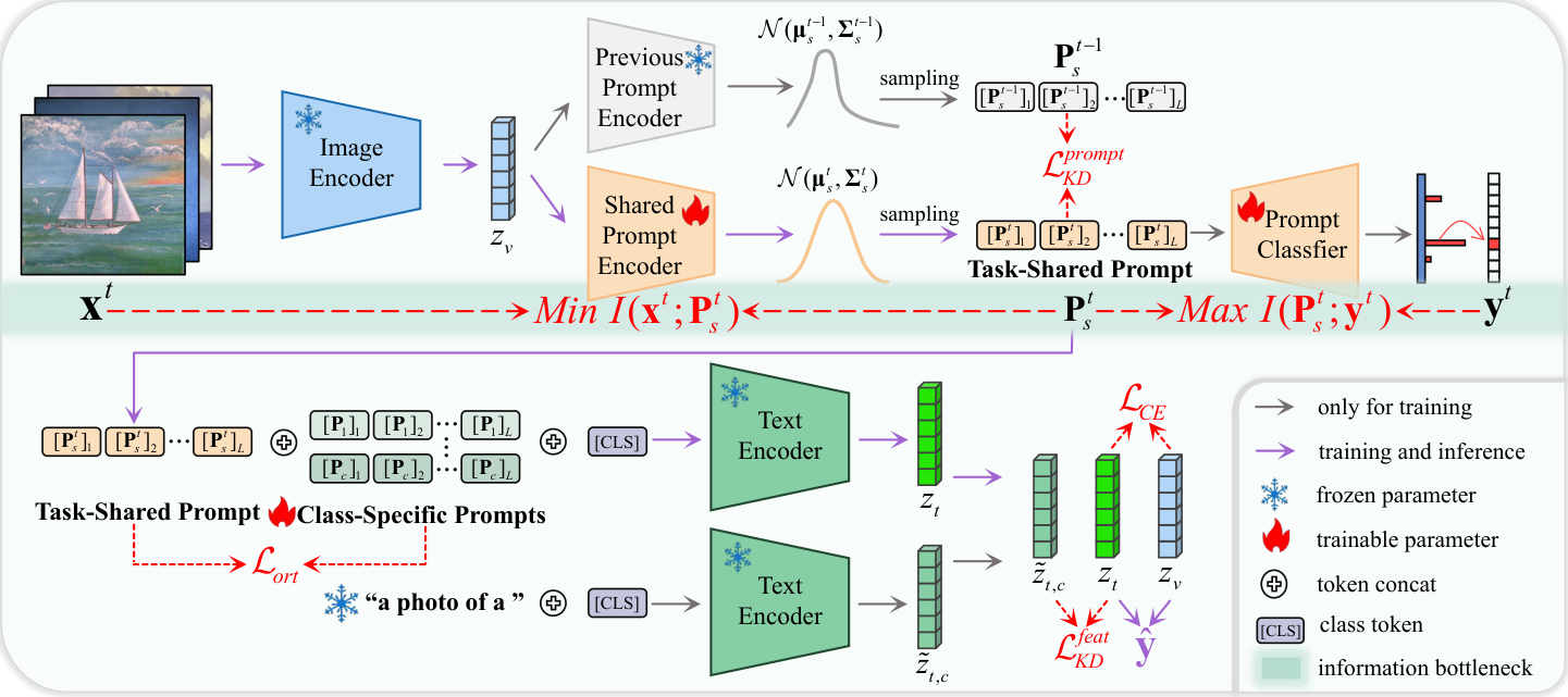
An alternative is to learn task-shared knowledge. For example, CoOp [50] continuously optimizes shared learnable prompts in the textual branch of CLIP, avoiding explicit prompt retrieval during inference. Nevertheless, without past task data, this strategy is prone to severe classifier bias [4, 44]: the shared prompts tend to overfit newly arrived tasks and misclassify past task samples into novel classes. Overall, existing prompt-based methods still suffer from retrieval dependence or classifier bias, limiting their potential to mitigate catastrophic forgetting in real-world CL settings. To address these challenges, we propose Decoupled Prompt Tuning for Continual Learning (DPT4CL), which decouples the prompt distribution into task-shared and class-specific components from an information-theoretic perspective, as shown in Fig. 1. This prompt design facilitates knowledge transfer across tasks while avoiding explicit prompt retrieval and alleviating classifier bias. The proposed DPT4CL consistently outperforms the zero-shot recognition baseline, Continual-CLIP [36], and existing prompt-based CL methods such as CoOp and AttriCLIP across the four datasets.
Specifically, DPT4CL decomposes the CLIP textual prompt space into two complementary components: a task-shared prompt distribution and class-specific prompts. The task-shared prompt distribution captures shared knowledge across sequential tasks. To this end, we leverage the Information Bottleneck (IB) principle to learn a compact yet sufficient unified prompt distribution by maximizing the mutual information (MI) between the prompt and class labels while minimizing the MI between input images and the prompt. This suppresses task-irrelevant visual redundancy while preserving discriminative task-shared semantics. We further introduce a distillation objective consisting of prompt-level distributional distillation and feature-level language-aware distillation to alleviate the classifier bias observed in CoOp-like prompt optimization. In parallel, class-specific prompts are introduced to encode category-specific semantics and enhance inter-class separability. Owing to the distinctive textual architecture of CLIP, each class-specific prompt can be directly associated with the [CLS] token of its corresponding category, avoiding task-specific prompt retrieval during inference. An orthogonalization objective is then employed to maximally disentangle class-specific prompts from the task-shared prompt. In this way, the task-shared prompt promotes stable cross-task knowledge transfer, while class-specific prompts strengthen local category discrimination, enabling DPT4CL to achieve state-of-the-art performance. Our main contributions are summarized as follows:
- •
We propose DPT4CL, a textual prompt tuning framework that decouples the CLIP textual prompt into a task-shared prompt distribution and class-specific prompts. The task-shared prompt distribution facilitates cross-task knowledge transfer, while distillation preserves semantic consistency to alleviate classifier bias. Meanwhile, class-specific prompts enhance inter-class separability through orthogonal decoupling from the task-shared prompt.
- •
We establish a unified excess risk bound through the lens of information theory, decomposing the overall risk into the Empirical Suboptimality Gap, Generalization Gap, and Forgetting. Our theoretical results formally demonstrate that the proposed decoupled prompt framework serves as a computationally tractable surrogate for controlling these critical quantities, thereby synergistically mitigating catastrophic forgetting and improving robust generalization.
- •
Extensive experiments on standard CL benchmarks demonstrate the effectiveness of DPT4CL. The proposed framework consistently outperforms strong zero-shot CLIP baselines and existing state-of-the-art CL methods.
II Related Work
II-A Continual learning
Existing continual learning scenarios can be broadly categorized into three settings [31]: task-incremental learning, where task identities are available during both training and inference [24, 11]; domain-incremental learning, where data distribution shifts while the task structure remains constant [30, 23]; and class-incremental learning, where new classes sequentially arrive and require the model to distinguish between all encountered classes without access to task identifiers [2]. Among these, class-incremental learning is the most challenging as it necessitates establishing a global decision boundary across all encountered classes, leading to inter-task interference and catastrophic forgetting. This has led to a proliferation of work aimed at designing classifiers to alleviate forgetting through functional regularization that penalizes critical changes to previous tasks [35, 19], modularized architectures that isolate task parameters [9, 22], and rehearsal strategies that retain data from previous tasks for joint training with the current task [29, 33]. Despite substantial progress, the performance of these methods often relies heavily on parameter-intensive modular expansion or the capacity of rehearsal buffers. In this paper, we address class-incremental learning with lightweight soft prompt tuning in a rehearsal-free setting, enabling effective use of pre-trained models while avoiding excessive parameter growth and memory dependence.
II-B Prompt-based continual learning
Recent extensive work has harnessed the powerful generalizability of pre-trained models by integrating them as backbones into CL frameworks [36, 21], thereby enhancing the model’s discriminative capability. However, in practice, their zero-shot performance often degrades on downstream out-of-domain data [43, 26]. Prompt tuning has emerged as a prevalent paradigm for efficient adaptation, which leverages learnable continuous tokens as inputs to the frozen visual and/or textual encoders to capture task-specific knowledge [50, 49]. For example, inspired by VPT [14], a series of vision-only prompt tuning CL approaches have been proposed. Among them, L2P [42] maintains a learnable visual prompt pool and utilizes a key-query matching strategy to dynamically retrieve instance-specific prompts, thereby effectively adapting to sequential tasks. DualPrompt [41] and CODA-Prompt [32] further advance this approach by incorporating complementary visual prompts into the pre-trained ViT backbone to capture rich task-specific information, thereby boosting performance. Meanwhile, benefiting from the rich semantic guidance provided by CLIP, an alternative line of textual soft prompt tuning approaches has emerged. For instance, methods such as CoOp [50] and AttriCLIP [40] adapt to CL scenarios by encapsulating task-relevant knowledge within textual prompts. Specifically, they employ learnable prompt vectors or prompt pool to extract linguistic semantics complementary to visual representations, thereby achieving favorable generalization across sequential tasks. Nevertheless, both vision-only prompt tuning and textual soft prompt tuning methods still suffer from the challenges of retrieval dependence or classifier bias, as discussed in the Introduction. In contrast to these approaches, we decouple the prompt distribution into task-shared and class-specific components from an information-theoretic perspective. This design facilitates effective transfer of task-shared knowledge while eliminating the dependence on explicit prompt retrieval during inference.
III Methodology
III-A Preliminaries
Continual learning (CL). Class-incremental CL aims to continuously learn knowledge of new classes from sequential tasks without forgetting knowledge of old classes. For each task , the dataset comprises pairs of input samples and their corresponding labels , drawn i.i.d. from the underlying data distribution over the joint space , where denotes the feature space and denotes the class space for task . For different tasks, the class spaces are typically disjoint, i.e., and , . When the -th task arrives, the learner accesses together with limited samples (if any) from previous tasks , with the objective of classifying samples over all observed classes .
CLIP-based prompt tuning. CLIP [27] contains an image encoder and a text encoder , which are jointly pre-trained on large-scale image-text pairs via a contrastive learning objective. Specifically, an image and a text are processed by encoders and to obtain the corresponding feature representations and . Here, is the sequence of text tokens derived from a prompt template such as the hand-crafted prompt “A photo of a [CLS]”, where [CLS] denotes a specific class label. By replacing [CLS] with each class name, we can obtain the set of text inputs , where denotes the total number of all observed classes. These inputs are then processed by the encoder to generate the corresponding representations . Consequently, the prediction probability for image belonging to the -th class can be computed by:
| (1) |
where is the cosine similarity, and is the temperature parameter.
To further enhance CLIP’s performance on the downstream tasks, CoOp [50] replaces hand-crafted prompts with a set of learnable textual soft prompts , where each denotes a learnable prompt vector. The resulting text prompt is then expressed by
| (2) |
Accordingly, the probability of classifying image as class is computed as:
| (3) |
where denotes the learnable prompt corresponding to class . Given the predicted probability distribution in Eq. (3), the cross-entropy (CE) loss is formulated as:
| (4) |
where is the binary ground-truth label (equal to 1 if belongs to class , and 0 otherwise).
Risk definition. To analyze our framework from the perspective of statistical learning theory, let denote the probabilistic mapping, parameterized by , from the input to the latent prompt , where is the continuous prompt space and is the parameter space of the encoder. Correspondingly, let denote the decoder, parameterized by , that projects the learned prompt to the class label, which mathematically abstracts the computation of Eq. (3). Here, denotes the parameter space of the decoder. After training on tasks , we denote the encoder parameters by and the decoder parameters by . The overall predictive distribution of classifying as class is defined as . Given a loss , the population and empirical risks on task are defined as
The forgetting on a previous task after training task is then formulated by
| (5) |
This measures the degree of performance degradation on task after sequentially training on tasks. Further, let denote the set of all measurable functions mapping the input space to the space of probability distributions over . We define the Bayes risk on task as , which quantifies the minimum expected risk achievable by an arbitrary predictive function over the true data distribution . Throughout our theoretical analysis, we focus on the overall excess risk across tasks, defined as:
| (6) |
which quantifies the discrepancy between the population risk of the learned model and that of the optimal functions in the hypothesis space . Here, the excess risk can be decomposed into three terms, where the Empirical Suboptimality Gap term measures how closely the empirical performance over tasks aligns with the theoretical best performance, the Generalization Gap characterizes the model’s ability to transfer knowledge learned on training data to unseen data, and the Forgetting reflects the magnitude of catastrophic forgetting incurred during incremental training.
III-B Framework of DPT4CL
Following the motivation discussed above, we present the concrete decoupling implementation of DPT4CL. Specifically, let and denote the task-shared prompt and class-specific prompts, respectively, where . These prompts are constrained to satisfy the following conditional independence with orthogonal constraints:
Proposition III.1.
A prompt is said to be maximally disentangled if the class-specific components , for are conditionally independent given the task-shared consensus . This implies a joint distribution , which is geometrically enforced by the constraint that the consensus subspace and all class-specific subspaces are mutually orthogonal.
To effectively capture the consensus component across different tasks, we employ the IB principle [37] to distill task-invariant consensus into the task-shared prompt distribution by maximizing the MI with the class label while minimizing the MI with the input image . This objective ensures that the learned distribution extracts the minimal sufficient statistics necessary for robust cross-task knowledge transfer, which is defined as:
| (7) |
where is the Lagrange multiplier and denotes MI. It is noteworthy that directly estimating the MI terms in Eq. (7) is computationally intractable in high-dimensional spaces. To this end, we adopt the variational formulation introduced in VIB [1] to derive a lower bound for the objective in Eq. (7). For brevity, we place the derivation in the Supplementary Material and only show the result of derivation:
| (8) |
where denotes the joint distribution of and , and is a variational approximation to the conditional distribution , which is parameterized by the prompt classifier illustrated in Fig. 2, and denotes the entropy of the class label. Since is independent of the parameter optimization and can thus be ignored, we can instead maximize the lower bound in Eq. (8) as a surrogate for directly optimizing . For the second term in Eq. (7), we also place the detailed derivation in the Supplementary Material and only present the result of derivation:
| (9) |
where denotes the KL divergence, while and are variational approximations to the conditional distribution and the marginal distribution , respectively. Here, we utilize a standard normal Gaussian distribution for the approximation, namely, , and assume that , where the mean and covariance are parameterized and learned via a task-shared prompt encoder [1, 39] as shown in Fig. 2.
Combining the above estimations, we can obtain a lower bound of the objective function in Eq. (7):
| (10) |
which serves as a tractable surrogate objective for learning the prompt distribution. Notably, the first term in Eq. (10) corresponds to the prompt classification loss, while the second term acts as a regularizer, encouraging the learned distribution to approximate the prior.
To mitigate classifier bias induced by independently optimizing the distribution parameters across tasks in a CoOp-like manner, we utilize a distribution distillation term that leverages the task-shared prompt to minimize the KL divergence between the current variational posterior and that from the previous task, thereby enforcing a unified task-shared prompt distribution. Furthermore, we introduce a language-aware distillation loss to align the text features derived from the learned prompts with the original feature space. This effectively mitigates cross-modal deviation [13] between the learned text representations and the frozen visual features, thereby preserving CLIP’s inherent representation power and preventing feature-level forgetting.
Specifically, consider the current learned distribution and the reparameterized task-shared prompt , along with their corresponding distribution and the reparameterized prompt from the end of the previous task , , where . The distillation loss can be formulated as:
| (11) |
where is the projected text representation of the -th class and denotes the corresponding hand-crafted prompt-based representation. Here, prompt-level distribution distillation penalizes the divergence of the prompt distribution, and feature-level language-aware distillation anchors the encoded text features to the original semantic space. Together, these two terms maintain semantic consistency across tasks and between modalities, thereby alleviating the classifier bias caused by CoOp-like prompt optimization.
Regarding the class-specific prompts for , we employ an orthogonalization objective to ensure that each prompt captures distinct, class-exclusive information while remaining strictly decoupled from the consensus knowledge preserved in the task-shared prompt . Specifically, we concatenate all prompt vectors into a matrix , and the objective is formulated as
| (12) |
serves as the structural constraint to ensure that the consensus knowledge and class-specific information encoded within the prompts are mutually orthogonal, as required by Proposition III.1, thereby promoting the learning of prompts that are both sufficient and maximally disentangled.
Consequently, by substituting the learnable prompt in Eq. (3) with the concatenation of the task-shared prompt and the class-specific prompt , the overall training objective for DPT4CL is formulated as:
| (13) |
where , , and are regularization coefficients.
During inference, a test image is first fed into the frozen image encoder to obtain its visual representation . Meanwhile, the shared prompt encoder samples the task-shared prompt conditioned on . For each observed class , the sampled task-shared prompt , the corresponding class-specific prompt , and the class token are concatenated and then fed into the text encoder to obtain the textual representation , where denotes the textual prompt constructed for class . The probability that belongs to the -th class is computed as
| (14) |
The final prediction is then given by
| (15) |
III-C Excess Risk Analysis
In this section, we establish a unified excess risk bound by separately controlling the Empirical Suboptimality Gap, Generalization Gap, and Forgetting terms in Eq. (6), thereby providing a rigorous theoretical guarantee for the proposed framework.
For each task , let denote the task-specific optimal population risk over the parameterized hypothesis spaces and , where the optimal parameters are defined as . Similarly, let denote the minimal sufficient statistic encoder obtained at the stationary point of the IB Lagrangian (7). Its corresponding Bayes risk under optimal decoding is denoted as . Based on the above definition, we have the following upper bound on the Empirical Suboptimality Gap:
Theorem III.2 (Empirical Suboptimality Gap).
Assume that the loss function is -Lipschitz continuous. For any , with probability at least over the datasets , we have
| (16) |
where , , and .
Remark III.3.
Theorem III.2 establishes the upper bound on the Empirical Suboptimality Gap, which is governed by the empirical optimization error , the IB representation error , and the irreducible architectural bias . These components provide a theoretical justification for the effectiveness of the proposed objectives (13) in improving performance. Specifically, quantifies the discrepancy between the learned model and the ideal hypothesis on the training set, capturing the optimization error inherent in the empirical training process. Given that the risk w.r.t the global population minimizer typically approaches zero, one can directly control by minimizing the empirical risk , which is exactly achieved by the cross-entropy objective in our framework.
Furthermore, characterizes representational discrepancy between the learned compressed latent representations and the ideal IB sufficient statistic . A large indicates the retention of task-irrelevant redundancy or the loss of task-discriminative information. This discrepancy is effectively mitigated by minimizing a variational upper bound of the IB Lagrangian, defined as in Eq. (10), which enforces a trade-off between compression and predictive precision.
The other factor measures the inherent structural bias between the IB-optimal trade-off and the non-parametric Bayes risk. This gap fundamentally arises from the inherent limitations of the parameterized prompt space in capturing the maximal sufficient statistic of the underlying data distribution. Specifically, by Fano’s inequality [7, 25], the classification error is lower-bounded by the conditional entropy , that is, the risk lower bound tightens as decreases. Given , maximizing the mutual information can effectively reduce , thereby tightening the risk lower bound. Hence, it is necessary to apply orthogonal constraints in (12) to capture sufficient, effective discriminative information while eliminating inter-prompt redundancy, mitigating the architectural approximation error relative to the non-parametric Bayes limit.
In the following theorem, we establish an upper bound on the Generalization Gap defined in Eq. (6) by leveraging the PAC-Bayesian framework.
Theorem III.4 (Generalization Gap).
Assume that the loss function is -Lipschitz continuous with respect to the model parameters. Let be the parameters learned at task . Let denote a data-dependent distribution over the parameter space centered at with an expected perturbation radius , such that . Let denote the corresponding prior distribution inherited from task , where is a data-independent initial prior. For any , with probability at least over the joint generation of datasets , we have
| (17) |
where is the Kullback-Leibler divergence.
Remark III.5.
Theorem III.4 suggests that the Generalization Gap is controlled by the PAC-Bayes complexity term, represented by the Kullback-Leibler divergence between the consecutive parameter distributions. Since direct optimization in the high-dimensional space is computationally intractable, we introduce distribution distillation as a tractable surrogate, which projects the parameter distributions onto the functional prompt-encoder space. This strategy effectively reduces the intractable parameter-level divergence into a computable divergence within the latent prompt space. In particular, for a given input , the divergence is evaluated between the reparameterized prompt distributions and , having which is formulated as the prompt-level regularization in the distillation loss in Eq. (11). Consequently, minimizing this regularizer can tighten the generalization bound, intrinsically mitigating catastrophic forgetting while facilitating task-shared knowledge transfer.
The following theorem provides the information-theoretic upper bound for the Forgetting term formulated in Eq. (6).
Theorem III.6 (Average Forgetting Bound).
Assume that the loss function is -Lipschitz continuous. Let and denote the encoder parameters learned at the task and a previous task . Under a task-specific decoder architecture where the decoder parameters assigned to task remain fixed during the training of subsequent tasks, the average catastrophic forgetting across all tasks is upper-bounded by:
| (18) |
Remark III.7.
Notably, Theorem III.6 reveals that the average forgetting is governed by the exact same KL divergence between the latent prompt distributions, i.e., , as the PAC-Bayesian complexity in Theorem III.4. Since directly optimizing the parameter drift in the high-dimensional space is computationally intractable, the prompt-level distillation term defined in Eq. (11) serves as a sufficient and tractable surrogate to effectively alleviate catastrophic forgetting. Additionally, to prevent these stable prompts from exhibiting cross-modal deviations, we empirically introduce the feature-level distillation term to constrain the learned prompts within the pre-trained semantic space. Consequently, minimizing the unified distillation loss in Eq. (11) both theoretically and empirically guarantees the ability to mitigate catastrophic forgetting while preserving the zero-shot recognition ability of pre-trained models.
IV Experiments
IV-A Implementation Details
IV-A1 Datasets
We evaluate our methods on four widely used CL benchmarks including CIFAR-100 [16], ImageNet-R [10], CUB-200 [38], and UCF-101 [34]. Following [47], we select classes from UCF-101 for evaluation. Detailed information and statistics of the datasets are provided in the Supplementary Material. For all datasets, we adopt a class-incremental setup with 10 tasks and report the average results over three random seeds. To ensure a fair comparison with prior work [5, 47], we additionally report the performance of all methods under the random seed 1993 in the Supplementary Material.
IV-A2 Evaluation metric
Overall average accuracy (Avg.), final accuracy (Last), and average forgetting measure (FM) are utilized to evaluate our model. Specifically, we adopt the Avg. and Last to quantify the generalization performance across all tasks, defined as and , respectively, where is the average accuracy over observed classes of tasks. Furthermore, we utilize the FM to quantify the extent of catastrophic forgetting on previously learned tasks, defined as , where denotes the maximum accuracy on task , and denotes the test accuracy of task after training on the final task . A lower FM indicates better retention of knowledge.
IV-A3 Baselines and compared methods
As summarized in Table I, we compare our proposed DPT4CL with a wide range of CL methods, which can be grouped into three categories: (1) Traditional CL methods. We adopt LwF [20], iCaRL [28], DER [45], and TagFex [46] as representative traditional CL competitors. (2) Prompt-based methods. Continual-CLIP [36] serves as the zero-shot recognition lower bound for CLIP-based methods. CoOp [50] learns only task-shared prompts in the textual branch of CLIP. AttriCLIP [40], L2P [42], DualPrompt [41], and CODA-Prompt [32] are included as representative methods that learn task-specific prompt pools. (3) CLIP-based SOTA methods. We compare with state-of-the-art CLIP-based methods, including CLAP4CLIP [13], ENGINE [47], and BOFA [18]. Additionally, to estimate the performance upper bound of our method, we evaluate DPT4CL under a joint-training setting, where all tasks are trained simultaneously and catastrophic forgetting is avoided.
IV-A4 Training details
We implement our method using PyTorch and conduct all experiments on an NVIDIA A800 GPU. To ensure a fair comparison, all compared methods are re-implemented with the same OpenAI-pre-trained CLIP ViT-B/16 backbone. For rehearsal-based methods, we use a fixed memory buffer of 2,000 samples, which are equally partitioned among all encountered classes. Optimization is performed using SGD, with momentum and weight decay set to 0.9 and 0.05, respectively. The learning rate is initialized to 0.05 and decayed by cosine annealing. For each incremental stage, the model is trained for 10 epochs with a batch size of 32. The reparameterization [1, 39] in Eq. (10) is implemented by a task-shared prompt encoder parameterized by a two-layer MLP, followed by a prompt classifier implemented by another two-layer MLP decoder, which is reinitialized at each new stage. The length of both the task-shared prompt and the class-specific prompt is fixed to 2. The dimension of each prompt vector is set to match the feature dimension of the pre-trained CLIP encoders for seamless multimodal interaction. Through grid search, the hyperparameters , , , and in Eqs. (10) and (13) are set to 0.5, , 1, and 10, respectively.
| Method | Memory | CIFAR-100 | ImageNet-R | CUB-200 | UCF-101 | ||||||||
|---|---|---|---|---|---|---|---|---|---|---|---|---|---|
| Avg. | Last | FM | Avg. | Last | FM | Avg. | Last | FM | Avg. | Last | FM | ||
| LwF [20] | 2000 | 40.90±3.69 | 28.75±4.27 | 32.93±0.96 | 26.92±2.87 | 19.02±2.13 | 20.50±1.18 | 20.15±6.48 | 14.72±3.30 | 21.22±4.20 | 42.50±6.19 | 24.55±2.58 | 45.99±2.01 |
| iCaRL [28] | 2000 | 45.51±7.82 | 27.67±9.71 | 54.43±3.49 | 23.93±13.26 | 11.17±6.80 | 21.96±8.80 | 44.84±12.67 | 35.74±11.28 | 18.79±2.34 | 79.19±8.79 | 69.16±10.66 | 19.77±6.56 |
| DER [45] | 2000 | 40.07±4.80 | 19.18±3.33 | 69.63±1.23 | 15.70±8.58 | 3.54±1.39 | 21.76±9.82 | 20.55±3.17 | 9.41±1.36 | 27.04±2.60 | 66.83±5.61 | 37.11±3.93 | 61.40±1.42 |
| TagFex [46] | 2000 | 57.74±8.24 | 49.11±4.32 | 45.88±0.80 | 13.03±2.34 | 3.52±0.59 | 19.73±3.54 | 14.00±4.37 | 5.20±0.55 | 22.20±4.10 | 63.95±4.08 | 35.82±3.04 | 62.14±2.17 |
| Continual-CLIP [36] | — | 78.79±0.32 | 68.37±0.03 | 8.67±1.01 | 79.74±0.45 | 72.98±0.00 | 9.02±0.96 | 64.70±1.32 | 53.29±0.07 | 12.95±2.96 | 74.92±1.80 | 66.33±0.04 | 9.59±0.57 |
| CoOp [50] | — | 77.22±0.39 | 64.89±2.23 | 18.98±2.30 | 81.83±0.43 | 74.32±1.73 | 9.98±1.01 | 64.08±1.02 | 47.57±2.87 | 23.16±2.96 | 76.07±0.79 | 64.04±0.34 | 27.48±1.88 |
| AttriCLIP [40] | — | 78.76±0.13 | 66.34±1.37 | 17.93±1.16 | 82.90±0.33 | 76.55±0.68 | 8.31±0.68 | 65.57±1.13 | 50.33±1.57 | 18.70±0.37 | 79.99±0.86 | 68.48±2.14 | 20.62±2.62 |
| L2P [42] | — | 80.73±1.13 | 68.07±1.24 | 8.60±2.06 | 76.83±1.33 | 66.95±2.23 | 13.38±1.93 | 65.84±1.57 | 52.52±1.06 | 16.43±3.58 | 84.52±0.69 | 75.47±0.16 | 14.71±2.35 |
| DualPrompt [41] | — | 83.07±1.01 | 73.04±0.53 | 6.02±0.94 | 82.53±0.73 | 75.68±0.74 | 9.40±0.54 | 70.88±1.84 | 58.59±1.51 | 15.77±1.50 | 91.32±1.17 | 84.82±0.91 | 7.28±1.37 |
| CODA-Prompt [32] | — | 83.48±0.76 | 72.04±1.43 | 16.81±1.48 | 82.54±0.21 | 74.47±0.44 | 9.83±0.94 | 72.04±1.55 | 58.23±1.00 | 19.86±1.75 | 88.90±1.19 | 80.69±0.83 | 15.72±0.94 |
| CLAP4CLIP [13] | 2000 | 83.85±0.29 | 75.04±0.43 | 9.04±0.68 | 84.19±0.38 | 78.57±0.30 | 6.86±0.96 | 74.66±0.70 | 64.79±0.99 | 12.45±2.97 | 91.88±0.32 | 84.91±0.38 | 6.12±0.50 |
| ENGINE [47] | — | 83.65±0.27 | 74.75±0.52 | 11.06±0.29 | 84.39±0.44 | 78.12±0.10 | 7.32±1.35 | 76.84±0.40 | 65.85±0.21 | 11.03±0.78 | 92.16±0.46 | 85.65±0.10 | 6.18±0.22 |
| BOFA [18] | — | 83.82±0.32 | 75.68±0.07 | 8.41±0.68 | 84.47±0.43 | 78.97±0.16 | 6.99±1.11 | 76.98±0.91 | 66.11±0.22 | 10.21±0.93 | 92.14±0.49 | 86.46±0.10 | 5.10±0.44 |
| Upper-bound | — | - | 80.91±0.06 | - | - | 81.46±0.12 | - | - | 73.46±0.38 | - | - | 94.97±0.21 | - |
| DPT4CL (ours) | — | 84.93±0.20 | 76.08±0.70 | 6.70±0.80 | 85.08±0.57 | 79.14±0.25 | 6.65±0.67 | 78.86±0.06 | 66.61±0.14 | 9.40±1.89 | 92.82±0.61 | 86.83±0.51 | 3.46±0.30 |
IV-B Benchmark Comparison
In this section, we evaluate DPT4CL against various representative and state-of-the-art methods on four widely used benchmarks under a 10-task class-incremental setting. The mean and standard deviation of Avg., Last, and FM over three random seeds are reported in Table I. Overall, DPT4CL achieves the best performance on 11 out of 12 evaluation metrics and the second-best performance on the remaining one, demonstrating its strong generalization and anti-forgetting capability across diverse CL scenarios.
IV-B1 Comparison with traditional CL methods
We first compare DPT4CL with traditional CL methods, including LwF, iCaRL, DER, and TagFex. Although all compared methods adopt the same pre-trained CLIP ViT-B/16 backbone for a fair comparison, DPT4CL substantially outperforms these traditional methods across all datasets and metrics. These results indicate that directly transferring conventional CL strategies to a CLIP-based backbone is still insufficient for class-incremental learning. In contrast, DPT4CL effectively exploits the semantic guidance of CLIP through textual prompt tuning, highlighting the importance of language-driven semantic adaptation in CL scenarios.
IV-B2 Comparison with prompt-based methods
We then compare DPT4CL with representative prompt-based CL methods. As shown in Table I, CoOp even underperforms Continual-CLIP on several datasets, especially in terms of Last accuracy. For instance, compared with Continual-CLIP, CoOp yields Last accuracy changes of , , and on CIFAR-100, CUB-200, and UCF-101, respectively, indicating that simply optimizing shared prompts can introduce severe classifier bias and degrade the model’s performance on previously learned tasks. In contrast, DPT4CL consistently improves over Continual-CLIP across all datasets, with average changes of in Avg. accuracy, in Last accuracy, and in FM over the four datasets. DPT4CL also consistently surpasses prompt pool methods, including AttriCLIP, L2P, DualPrompt, and CODA-Prompt. Unlike these methods, which rely on query–key matching to retrieve task-specific prompts during inference, DPT4CL decouples the learnable textual prompt into task-shared and class-specific components. This design avoids explicit prompt retrieval while preserving cross-task transferable knowledge and category-level discrimination, demonstrating the effectiveness of DPT4CL as a new prompt-based CL paradigm.
IV-B3 Comparison with CLIP-based SOTA methods
We further compare DPT4CL with recent CLIP-based SOTA methods, including adapter-based methods such as CLAP4CLIP and ENGINE, and the LoRA-based method BOFA. As shown in Table I, DPT4CL achieves superior performance over these methods, particularly in terms of FM. For example, DPT4CL obtains the lowest FM of 3.46% on UCF-101, demonstrating its strong ability to mitigate catastrophic forgetting. This further validates the effectiveness of the IB-based decoupling strategy in preserving task-shared consensus knowledge while learning class-specific semantics. Since DPT4CL performs adaptation only in the input-space, it is potentially complementary to feature-space adaptation strategies such as adapter-based and LoRA-based fine-tuning. For example, CLAP4CLIP could further benefit from replacing its textual prompt tuning component with more advanced designs. This leaves room for future work on jointly optimizing DPT4CL with feature-space adaptation for CLIP-based continual learning.
IV-B4 Comparison with rehearsal-based methods
Finally, compared with rehearsal-based methods, such as LwF, iCaRL, DER, TagFex, and CLAP4CLIP, DPT4CL is rehearsal-free. Despite using no stored exemplars from previous tasks, it achieves markedly better performance on most benchmarks. This highlights the efficiency of DPT4CL in resource-constrained scenarios, where storing or revisiting previous data may be infeasible due to memory, privacy, or deployment constraints.
| Variants | Avg. () | Last () | FM () |
|---|---|---|---|
| Baseline (CoOp) | 77.22±0.39 | 64.89±2.23 | 18.98±2.30 |
| Only task-shared prompt | 81.10±0.69 | 70.78±0.36 | 9.29±0.89 |
| Only class-specific prompts | 82.77±0.39 | 73.73±0.28 | 7.64±0.68 |
| DPT4CL w/o | 83.30±0.63 | 73.26±0.79 | 8.41±0.57 |
| DPT4CL w/o | 84.55±0.24 | 75.56±0.26 | 7.46±1.03 |
| DPT4CL | 84.93±0.20 | 76.08±0.70 | 6.70±0.80 |
IV-C Further Analysis
IV-C1 Ablation Study
To evaluate the contribution of each component in Eq. (13), we conduct an ablation study on CIFAR-100. As shown in Table II, when only applying , the framework degenerates to the baseline CoOp, yielding suboptimal average accuracy and severe forgetting. The variant Only task-shared prompt learns only the task-shared prompt distribution through the IB objective on top of , while Only class-specific prompts introduces only class-specific prompts and the corresponding orthogonalization loss based on . Moreover, DPT4CL w/o and DPT4CL w/o are used to investigate the effects of removing and from the complete framework, respectively. With all components jointly optimized, DPT4CL achieves the best Avg. accuracy of 84.93%, Last accuracy of 76.08%, and FM of 6.70%, validating the complementary contributions of these components.
| Length of prompt | CIFAR-100 | UCF-101 | ||||
|---|---|---|---|---|---|---|
| Avg. | Last | FM | Avg. | Last | FM | |
| 1 | 84.39±0.41 | 75.50±0.23 | 6.79±0.60 | 92.58±0.52 | 86.49±0.33 | 4.12±0.16 |
| 2 | 84.93±0.17 | 76.08±0.57 | 6.70±0.66 | 92.82±0.50 | 86.83±0.42 | 3.46±0.24 |
| 3 | 84.85±0.20 | 76.06±0.25 | 7.83±0.75 | 93.07±0.18 | 87.31±0.67 | 3.55±0.21 |
| 4 | 84.86±0.21 | 75.94±0.24 | 6.94±0.39 | 92.79±0.35 | 86.79±0.98 | 3.57±0.30 |
IV-C2 Hyperparameter analysis
We conduct a sensitivity analysis on the prompt length , which denotes the length of both the task-shared prompt and the class-specific prompts. As shown in Table III, DPT4CL achieves stable performance across different values of on CIFAR-100 and UCF-101. In particular, yields the best overall trade-off, achieving the best results on CIFAR-100 and the lowest FM on UCF-101, while larger prompt lengths bring no consistent performance gains. Therefore, we set as the default configuration for all benchmarks. Detailed analyses for the remaining loss coefficient hyperparameters (, , , and ) are provided in the Supplementary Material.
IV-C3 Parameter count analysis
Fig. 3 compares the learnable parameter growth of DPT4CL with CLIP-based SOTA methods on CIFAR-100. With a ViT-B/16 backbone and prompt dimension , DPT4CL introduces about 3.68M task-shared parameters from the prompt encoder and classifier. Its incremental parameters only come from class-specific prompts for newly arrived classes. Since each task contains 10 new classes, DPT4CL adds only parameters per task, i.e., about 0.01M when . In contrast, CLAP4CLIP and ENGINE introduce adapter-style modules with parameters per task. Thus, DPT4CL requires only about of their incremental parameters, demonstrating better parameter efficiency and scalability while achieving superior performance in Table I.
| (a) DPT4CL task-shared prompt | (b) DPT4CL concatenated prompts |
IV-C4 Visualization analysis
We visualize the learned prompts of DPT4CL on CIFAR-100 using t-SNE. As shown in Fig. 4(a), the task-shared prompts form a continuous manifold in the prompt space, indicating that they capture shared knowledge transferred across different tasks. Fig. 4(b) shows that the complete prompts obtained by concatenating the task-shared prompt with class-specific prompts exhibit a more discrete distribution with enlarged inter-class margins in the prompt space, suggesting that the class-specific prompts introduce additional category-discriminative information.
To further analyze the classifier bias caused by CoOp-like prompt optimization, we compare the final task-wise accuracy of CoOp and DPT4CL on CIFAR-100 after training all 10 tasks. As shown in Fig. 5, CoOp exhibits clear performance degradation on old tasks, while DPT4CL achieves consistently higher accuracy on most previously learned tasks. These results demonstrate that the proposed decoupled prompt design effectively alleviates classifier bias and better preserves knowledge from previous tasks.
V Conclusion
In this paper, we propose DPT4CL, a rehearsal-free prompt tuning framework for CLIP-based continual learning. Different from existing prompt-based methods, DPT4CL provides a new prompt tuning paradigm for CL by decoupling the prompt design into task-shared and class-specific components, thereby avoiding explicit prompt retrieval while maintaining effective knowledge transfer and discriminative prompt representations across sequential tasks. Extensive experiments on four standard CL benchmarks demonstrate the effectiveness of DPT4CL, which achieves the best performance on 11 out of 12 evaluation metrics and the second-best performance on the remaining one. Moreover, the proposed framework is supported by a unified excess risk analysis from an information-theoretic perspective, providing theoretical insight into its ability to control generalization and forgetting. In addition, its rehearsal-free nature and small incremental parameter cost make it suitable for resource-constrained scenarios. In future work, we will explore the joint optimization of input-space prompt tuning and feature-space adaptation strategies for CL.
References
- [1] (2017) Deep variational information bottleneck. International Conference on Learning Representations. External Links: Document Cited by: §III-B, §III-B, §IV-A4.
- [2] (2021) A comprehensive study of class incremental learning algorithms for visual tasks. Neural Networks 135, pp. 38–54. External Links: Document Cited by: §II-A.
- [3] (2019) On tiny episodic memories in continual learning. arXiv preprint arXiv:1902.10486. External Links: Document Cited by: §I.
- [4] (2025) Adaptive retention & correction: test-time training for continual learning. In International Conference on Learning Representations, External Links: Document Cited by: §I.
- [5] (2025) Preserving cross-modal consistency for clip-based class-incremental learning. arXiv preprint arXiv:2511.10974. External Links: Document Cited by: §IV-A1.
- [6] (2022) AdaptFormer: adapting vision transformers for scalable visual recognition. In Advances in Neural Information Processing Systems, Vol. 35, pp. 16664–16678. Cited by: §I.
- [7] (1999) Elements of information theory. John Wiley & Sons. Cited by: Remark III.3.
- [8] (2021) An image is worth 16x16 words: transformers for image recognition at scale. In International Conference on Learning Representations, External Links: Document Cited by: §I.
- [9] (2022) Dytox: transformers for continual learning with dynamic token expansion. In Proceedings of the IEEE/CVF Conference on Computer Vision and Pattern Recognition, pp. 9285–9295. External Links: Document Cited by: §II-A.
- [10] (2021) The many faces of robustness: a critical analysis of out-of-distribution generalization. In Proceedings of the IEEE/CVF International Conference on Computer Vision, pp. 8340–8349. External Links: Document Cited by: §IV-A1.
- [11] (2022) Rethinking task-incremental learning baselines. In 2022 26th International Conference on Pattern Recognition (ICPR), pp. 2771–2777. External Links: Document Cited by: §II-A.
- [12] (2022) LoRA: low-rank adaptation of large language models. In International Conference on Learning Representations, Cited by: §I.
- [13] (2024) Clap4clip: continual learning with probabilistic finetuning for vision-language models. Advances in Neural Information Processing Systems 37, pp. 129146–129186. External Links: Document Cited by: §I, §III-B, §IV-A3, TABLE I.
- [14] (2022) Visual prompt tuning. In European Conference on Computer Vision, pp. 709–727. External Links: Document Cited by: §II-B.
- [15] (2017) Overcoming catastrophic forgetting in neural networks. Proceedings of the National Academy of Sciences 114 (13), pp. 3521–3526. External Links: Document Cited by: §I.
- [16] (2009) Learning multiple layers of features from tiny images. Technical report Cited by: §IV-A1.
- [17] (2023) LiFT: transfer learning in vision-language models for downstream adaptation and generalization. In Proceedings of the 31st ACM International Conference on Multimedia, pp. 4678–4687. External Links: Document Cited by: §I.
- [18] (2026) Bofa: bridge-layer orthogonal low-rank fusion for clip-based class-incremental learning. In Proceedings of the AAAI Conference on Artificial Intelligence, Vol. 40, pp. 22967–22975. Cited by: §IV-A3, TABLE I.
- [19] (2024) Continual learning with knowledge distillation: a survey. IEEE Transactions on Neural Networks and Learning Systems 36 (6), pp. 9798–9818. External Links: Document Cited by: §II-A.
- [20] (2018) Learning without forgetting. IEEE Transactions on Pattern Analysis and Machine Intelligence 40 (12), pp. 2935–2947. External Links: Document Cited by: §IV-A3, TABLE I.
- [21] (2025) C-clip: multimodal continual learning for vision-language model. In The Thirteenth International Conference on Learning Representations, Cited by: §II-B.
- [22] (2025) LoRA subtraction for drift-resistant space in exemplar-free continual learning. In Proceedings of the Computer Vision and Pattern Recognition Conference, pp. 15308–15318. External Links: Document Cited by: §II-A.
- [23] (2026) Domain incremental learning for object detection. Pattern Recognition 170, pp. 111882. External Links: Document Cited by: §II-A.
- [24] (2021) Ternary feature masks: zero-forgetting for task-incremental learning. In Proceedings of the IEEE/CVF Conference on Computer Vision and Pattern Recognition, pp. 3570–3579. External Links: Document Cited by: §II-A.
- [25] (2025) Minimum-error state discrimination and fano’s inequality. American Journal of Physics 93 (7), pp. 566–573. Cited by: Remark III.3.
- [26] (2023) Combined scaling for zero-shot transfer learning. Neurocomputing 555, pp. 126658. External Links: Document Cited by: §II-B.
- [27] (2021) Learning transferable visual models from natural language supervision. In International Conference on Machine Learning, pp. 8748–8763. External Links: Document Cited by: §I, §III-A.
- [28] (2017) ICaRL: incremental classifier and representation learning. In IEEE Conference on Computer Vision and Pattern Recognition, pp. 5533–5542. External Links: Document Cited by: §IV-A3, TABLE I.
- [29] (2019) Experience replay for continual learning. Advances in Neural Information Processing Systems 32. External Links: Document Cited by: §II-A.
- [30] (2023) A unified approach to domain incremental learning with memory: theory and algorithm. Advances in Neural Information Processing Systems 36, pp. 15027–15059. External Links: Document Cited by: §II-A.
- [31] (2025) Continual learning of large language models: a comprehensive survey. ACM Computing Surveys 58 (5), pp. 1–42. External Links: Document Cited by: §I, §II-A.
- [32] (2023) Coda-prompt: continual decomposed attention-based prompting for rehearsal-free continual learning. In Proceedings of the IEEE/CVF Conference on Computer Vision and Pattern Recognition, pp. 11909–11919. External Links: Document Cited by: §I, §II-B, §IV-A3, TABLE I.
- [33] (2024) Adaptive memory replay for continual learning. In Proceedings of the IEEE/CVF Conference on Computer Vision and Pattern Recognition, pp. 3605–3615. External Links: Document Cited by: §II-A.
- [34] (2012) UCF101: a dataset of 101 human actions classes from videos in the wild. arXiv preprint arXiv:1212.0402. External Links: Document Cited by: §IV-A1.
- [35] (2023) Regularizing second-order influences for continual learning. In Proceedings of the IEEE/CVF Conference on Computer Vision and Pattern Recognition, pp. 20166–20175. External Links: Document Cited by: §II-A.
- [36] (2022) Clip model is an efficient continual learner. arXiv preprint arXiv:2210.03114. External Links: Document Cited by: §I, §II-B, §IV-A3, TABLE I.
- [37] (2000) The information bottleneck method. arXiv preprint physics/0004057. External Links: Document Cited by: §III-B.
- [38] (2011) The caltech-ucsd birds-200-2011 dataset. Technical report Technical Report CNS-TR-2011-001. Cited by: §IV-A1.
- [39] (2019) Deep multi-view information bottleneck. In Proceedings of the 2019 SIAM International Conference on Data Mining, pp. 37–45. External Links: Document Cited by: §III-B, §IV-A4.
- [40] (2023) Attriclip: a non-incremental learner for incremental knowledge learning. In Proceedings of the IEEE/CVF Conference on Computer Vision and Pattern Recognition, pp. 3654–3663. External Links: Document Cited by: §I, §II-B, §IV-A3, TABLE I.
- [41] (2022) Dualprompt: complementary prompting for rehearsal-free continual learning. In European Conference on Computer Vision, pp. 631–648. External Links: Document Cited by: §I, §II-B, §IV-A3, TABLE I.
- [42] (2022) Learning to prompt for continual learning. In Proceedings of the IEEE/CVF Conference on Computer Vision and Pattern Recognition, pp. 139–149. External Links: Document Cited by: §I, §II-B, §IV-A3, TABLE I.
- [43] (2022) Robust fine-tuning of zero-shot models. In Proceedings of the IEEE/CVF Conference on Computer Vision and Pattern Recognition, pp. 7959–7971. External Links: Document Cited by: §II-B.
- [44] (2019) Large scale incremental learning. In Proceedings of the IEEE/CVF Conference on Computer Vision and Pattern Recognition, External Links: Document Cited by: §I.
- [45] (2021) DER: dynamically expandable representation for class incremental learning. In IEEE/CVF Conference on Computer Vision and Pattern Recognition, pp. 3013–3022. External Links: Document Cited by: §IV-A3, TABLE I.
- [46] (2025) Task-agnostic guided feature expansion for class-incremental learning. In IEEE/CVF Conference on Computer Vision and Pattern Recognition, pp. 10099–10109. External Links: Document Cited by: §IV-A3, TABLE I.
- [47] (2025) External knowledge injection for clip-based class-incremental learning. In Proceedings of the IEEE/CVF International Conference on Computer Vision, pp. 3314–3325. External Links: Document Cited by: §IV-A1, §IV-A3, TABLE I.
- [48] (2024) Class-incremental learning: a survey. IEEE Transactions on Pattern Analysis and Machine Intelligence. External Links: Document Cited by: §I.
- [49] (2022) Conditional prompt learning for vision-language models. In Proceedings of the IEEE/CVF Conference on Computer Vision and Pattern Recognition, pp. 16816–16825. External Links: Document Cited by: §II-B.
- [50] (2022) Learning to prompt for vision-language models. International Journal of Computer Vision 130 (9), pp. 2337–2348. External Links: Document Cited by: §I, §II-B, §III-A, §IV-A3, TABLE I.