Knots and the Sierpinski tetrahedron

Journal: ArXiv

Malors Espinosa Email: espino41@mail.tsinghua.edu.cn, Yau Mathematical Science Center, Tsinghua University

Abstract

In this paper we prove that there are infinitely many knots that cannot be embedded in the $1$ -skeletons of the finite iterations of the Sierpinski tetrahedron fractal. We do this by proving that such an embedding induces a sphere decomposition of weight at most $6$ . There are infinitely many knots with spherewidth greater than this.

Mathematics Subject Classification: 57K10, 28A80

1 Introduction

1.1 Motivation and main results

The Sierpinski tetrahedron is a fractal constructed out of an iterative process. Concretely, a regular solid tetrahedron gets substituted by its homothetic copies, with proportion of 1/2, at each one of its vertices. At each step, this substitution is carried out on each remaining solid tetrahedrons. The intersection of this sequence of nested closed sets is the fractal.

Refer to caption — Figure 1: The different iteration stages of the construction

The 1-skeletons of the finite stages is a particular sequence of graphs, all of which are subsets of the Sierpinski tetrahedron. We see from this that this fractal has embedded many polygonal curves.

In [1] we looked for some of these polygonal curves that were knotted. In other words, we wondered whether all (tame) knots can be found as subsets of the Sierpinski tetrahedron. Our strategy was to find the knots as subpaths of some big enough 1-skeleton. This then implies it is also in the fractal itself.

We were able to prove that all Pretzel knots can be found in the 1-skeletons. We conjectured that, in fact, all knots should be there in the final fractal. The purpose of this paper is to prove the following result.

Theorem A.

Let $T(p,q)$ be a torus knot with $\min\{p,q\}>9$ , then $T(p,q)$ cannot be embedded in the $1$ -skeleton of a finite iteration of the Sierpinski tetrahedron. In particular, there are infinitely many knots that cannot be embedded in the $1$ -skeletons of the finite iterations of the Sierpinski tetrahedron.

This theorem does not answer completely whether all knots are in the Sierpinski tetrahedron, but it certainly casts doubts on the veracity of the claim. When we looked for Pretzel knots, for the results of [1], we did it by a combinatorial search. There didn’t seem to be any major reason why a more patient and methodical search would not be able to lead to any given knot. Now we know that, if some version of the conjecture is true, there will need to be tame knots that indeed use the fractal structure of the Sierpinski tetrahedron to avoid the restrictions the finite iterations pose.

However, in the quest of understanding tame knots that we find with wild presentations, the fractal is very misleading and at the moment I don’t know if the results of this work generalize in some way or if there are genuinely new knots to be found in the Sierpinski tetrahedron but not a moment before.

The main constructions that serves our proof are sphere decompositions and the spherewidth of a knot. Following [5], we have the following two definitions.

Definition A.

A thickened embedding of a graph $G$ is an embedding of $G$ in $\mathbb{S}^{3}$ where each vertex is thickened to a small ball. Two balls are connected by a polygonal edge if an only if they are adjacent in the graph $G$ , and pairs of edges are disjoint.

Definition B.

Let $G$ be a graph thickly embedded in $\mathbb{S}^{3}$ . A sphere decomposition of $G$ is a continuous map $f\mathrel{\mathop{\mathchar 58\relax}}\mathbb{S}^{3}\longrightarrow\mathcal{T}$ where $\mathcal{T}$ is a trivalent tree with at least one edge. It satisfies

(SD 1): For all $x\in L(\mathcal{T})$ , $f^{-1}(x)$ is a point disjoint from $G$ .
(SD 2): For all $x\in V(\mathcal{T})-L(\mathcal{T})$ , $f^{-1}(x)$ is a double bubble transverse to $G$ .
(SD 3): For all $x\in\mathcal{T}$ interior to an edge, $f^{-1}(x)$ is a sphere transverse or finitely tangent to $G$ .

You can see examples of double bubbles in figures 4 and 5. We then have

Definition C.

Let $G$ be a graph and $f\mathrel{\mathop{\mathchar 58\relax}}\mathbb{S}^{3}\longrightarrow\mathcal{T}$ be a sphere decomposition of $G$ . We define the width of $f$ as the supremum of the weights of the spheres $f^{-1}(x)$ for all $x$ interior to the edges. That is,

w(f)\mathrel{\mathop{\mathchar 58\relax}}=\displaystyle\sup_{x\in G-V(G)}w(f^{-1}(x)).

Furthermore, the spherewidth of $G$ is the infimum of the widths of its sphere decompositions. That is,

sw(G)\mathrel{\mathop{\mathchar 58\relax}}=\displaystyle\inf_{f\mathrel{\mathop{\mathchar 58\relax}}\mathbb{S}^{3}\longrightarrow\mathcal{T}}w(f).

In the above definition, the weight of a sphere $S$ with respect to $G$ is the number of connected components of $G\cap S$ .

In vague terms, a sphere decomposition is a “movie” that shows the growth of several spheres. They start as points, they grow and merge, and eventually they become a single sphere that grows towards infinity. This movie is not parametrized by time, but by the trivalent tree $\mathcal{T}$ . If you were to stop at any point of the interior of the edges, you would see a snapshot of how a sphere is growing. In the process of growth, these spheres hold in their interior part of the given knot until they hold it entirely.

The knot is a single component, however, as the spheres grow they might collect different parts of the knot that are disconnected and will only merge at a later point. The spherewidth $sw(K)$ of a knot $K$ , then, is an unavoidable quality of the sphere growth: no matter how you run this process, somewhere along the way, at least one of the spheres intersected the knot at least a certain fixed amount of times.

Consequently, if one is able to produce a sphere decomposition where at every point, interior to the edges of $\mathcal{T}$ , the number of components, in the intersections with the knot, is bounded above by an absolute constant, then the spherewidth is bounded above by this same constant.

We prove the following result.

Theorem B.

Let $K$ be a knot that can be embedded in a finite iteration of the Sierpinski tetrahedron. Then $K$ admits a sphere decomposition of weight at most $6$ .

Theorem A follows from theorem B because it is known (see [5]) that

sw(T(p,q))\geq\dfrac{2}{3}\min\{p,q\}.

Theorem B follows by constructing an specific sphere decomposition from a finite iteration and the way the knot embeds in its $1$ -skeleton. Intuitively, this sphere decomposition is very clear. We see “snapshots” of this growth when we pick an iteration, from the zeroth one up to the one that includes the knot, and take as bubbles the tetrahedrons themselves. The challenge lies on proving that these snapshots are indeed part of a larger picture (i.e. one can build the sphere decomposition out of this data). Finally, the reason why the absolute bound is achieved is that every tetrahedron can contain at most two connected components of the knot (because there are only four vertices!). Thus, no matter how one tetrahedron grows into a bigger one, the components must glue together into at most two components. This constrain limits severely how the number of components can grow within a single sphere.

1.2 Organization of this paper

In our paper we will work with polyhedrons. In section 2 we will review some properties and definitions we need from them. This section is complemented in the A where one of our main construction results is proven. We put this in an appendix to do not break the flow of the argument, having in mind that what is required there is not used, beyond the result itself, for the rest of the paper.

The choice of working on polyhedrons was taken by the author after trying to do all this somewhat explicitly within the smooth category. Nothing was really problematic except to guarantee that, at every stage that is needed, one can satisfy the conditions of transversality or finite tangency. I could not find a result that properly stated that all the constructions I was making did not, at some unfortunate point, created problems due to how it altered the knot. I am sure most of this constitutes nothing else than my own limitations on the knowledge of the area. On top of this, A.I. was screaming at me that this was absolutely true and known to everyone, except obviously me. This gave me pause and I decided to simply work with polyhedrons. I apologize if I overcomplicated the task without need.

In section 3 we review the concepts of sphere decompositions and of spherewidth. We follow the work of [5] for this. In section 4 we prove theorem A and theorem B. This is a long section. We begin by modifying the construction of the finite iterations with tetrahedrons with a different one which, eventually, will let us to work with cubes. Then we will explain how to obtain the combinatorial information necessary to construct the sphere decomposition. We do this carefully to be able to control the growth of components within intermediate stages of the growth process. In here, we put special attention to the particular thickening of the vertices. We do this to make sure they do not make our bounds grow because we chose a bad construction.

In section 5 we make a concrete example with the trefoil. Our objective is to show that from the data of the embedding into a finite iteration one can indeed very easily read all the information needed to compute the sphere decompositon.

Finally, in 6 we pose two questions that follow from this work and that the author finds interesting.

1.3 Discussion on some previous literature and some comments

During this work we will be assuming that the reader is familiar with the required contents of [1]. The authors of the aforementioned paper, at the time of writing it, could not find a lot of material relating knots and fractals in the way we were interested in. Since then, some related results have appeared and some new information has been made available to the author.

To begin with, the work of Shtan’ko, [7], settles the existence of knots already embedded in the Menger Sponge. However, it does it in a nonconstructive way and does not deal with the skeletons of the finite iterations, as we did in [1]. The author was lead to this bibliography by none other than ChatGPT as we will discuss in our A.I. disclosure. Besides tame knots, the work of Shtan’ko also deals with wild knots, but once more does not do the embedding constructively. The recent work of Hinojosa, Morales-Fuentes, Valdez and Verjovsky, [2], deals with some of them in a constructive way.

As far as my understanding goes, the results of Shtan’ko do not extend to the Sierpinski tetrahedron and thus do not complete our quest to know what happens in the fractal itself. Furthermore, I could not find (even with help of A.I.) literature that would immediately imply this result was already established for some unknown reason to me.

Related to our main tool, sphere decompositions, the main work we use is Lunel’s and De Mesmay’s, [5]. The idea, as we have mentioned before, is to understand how a knot can be “isolated” in growing spheres. However, similar ideas can be applied to knot diagrams. In particular, the concept of tree decompositions, as developed in the work of De Mesmay, Purcell, Schleimer and Sedgwick, [6], is an approach the author tried but could not make work. The difference is that, when dealing with the knot diagrams that come from the combinatorial representations (see figure 12), there are intersections that are really not there. They are simply the price to pay for flattening a highly non planar object. Thus, when trying to build bags, as in [6, Definition 2.1], with controlled size, these crossings made my bounds to not be uniform. This problem is what motivated me to try directly with the 3D version of the problem, which at first I tried to avoid.

For some nice examples of what happens when one deals with wild knots versus tame knots, I found Kobayashi’s, [4], very illuminating.

1.4 A.I. use disclosure

In the process of writing this paper I have used ChatGPT and Deepseek. I am writing this introduction on the same week that the Navier-Stokes controversy is developing and I find it’s best to be explicit with what we did and know with A.I.

ChatGPT Pro, the 20 dollar version, is what I used. I used it twice. The first time was to discuss the original result I wanted to prove. I discussed my main ideas on how one can possibly prove all knots were in the finite iterations. Nothing of depth ocurred. We discussed also the result of the Menger Sponge proven in [1] with the hopes of adapting it to the Sierpinski. It is here where ChatGPT showed me Shtan’ko’s work [7]. I wonder if it told me this because it was mentioned in the introduction of [2]. I became aware of this latter paper by other means.

I eventually confessed to ChatGPT that recently I have doubted the conjecture to be true. I quote myself: “I do not know enough of knot theory to say this precisely, but I can imagine that there are knots that are REALLY knotted and thus any knot representative cramps no matter what you do. Hence, the connectivity of the Sierpinski simply does not give enough.” (Yes, I used cramps and I meant piles up. I cannot explain.) At this comment, ChatGPT thought for a bit and referred to me to the concepts of spherewidth, sphere decompositions and tree decompositions, as well as the papers [5], [6]. Never before I have heard any of this.

It mentioned that my “cramped” knots would be torus knots and showed me the known lower bounds. We discussed for a long while because I could not grasp in its entirety all that it was explaining to me, but ultimately it turned into a plan of attack that became the backbone of what I present in this paper. I decided not to use more of ChatGPT for this project because I wanted to solidify the rest myself.

The second time I used ChatGPT was to know suggestions of programs I could use to make many of the several pictures you will see in this paper. It suggested many, among them Asymptote, which became extremely valuable. I did this because Deepseek did not suggest any option that seemed a good idea.

For the rest of the process, I worked with the free version of Deepseek. I used it to generate the codes to create the images in Asymptote. It helped me to do the tikz diagrams. It helped me to verify certain computational details in the propositions of the A. It also told me several results related to transversality in sphere decompositions are well known and provided me several sources. However, I did check this bibliography and I could not see in an straightforward way what I wanted.

I have found working and learning with A.I. fascinating. It is deeply discouraging and somewhat painful to see what it is becoming.

1.5 Ackwonledgements

I take the opportunity to thank the mathematical community, whether researchers, educators or students, for their unexpected support in our work on knots and fractals.

2 Some geometric observations on polyhedra

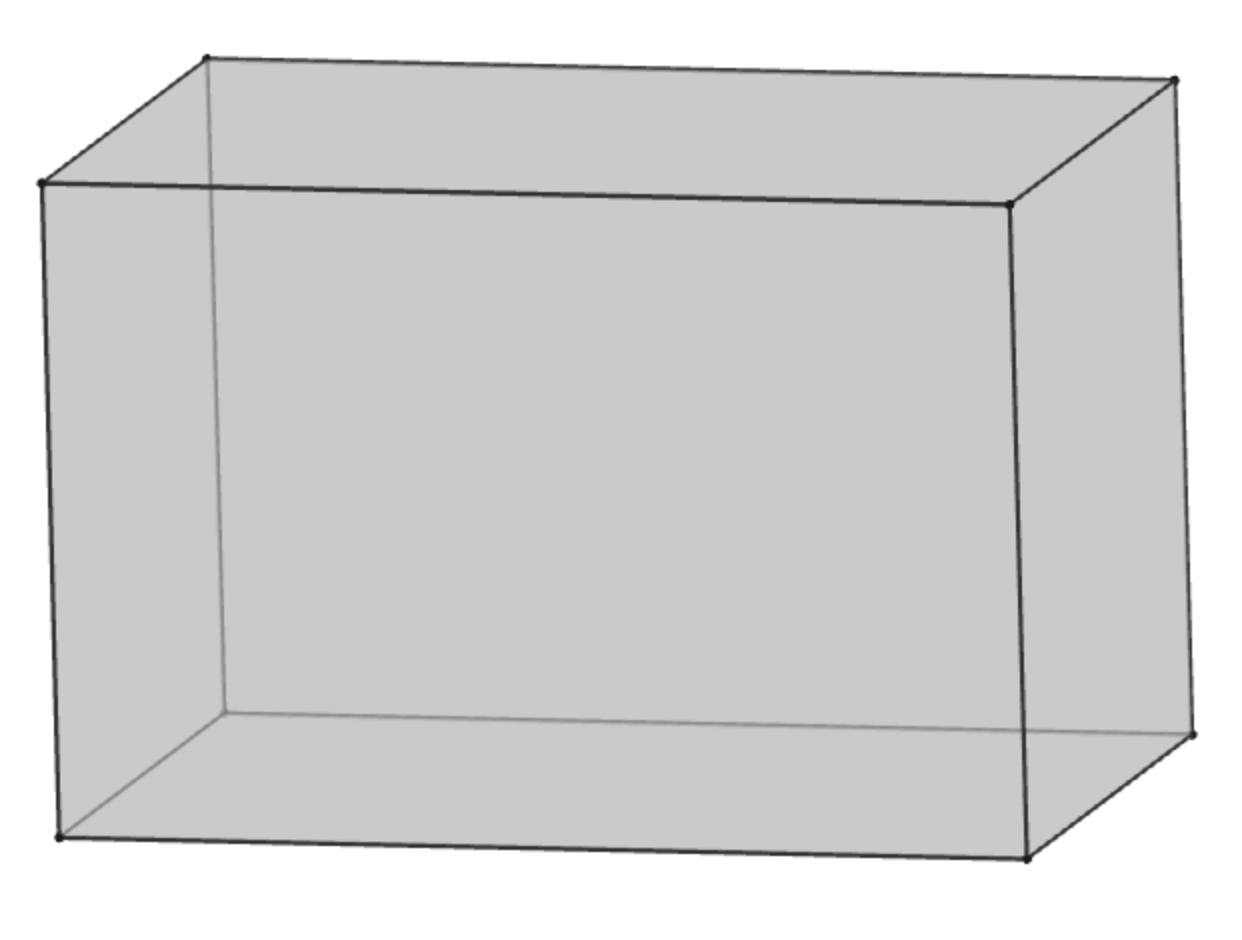
Throughout the paper, including A, we will prominently refer to two families of polyhedra. We will agree that their definition is understood by the following drawings together with some brief explanations about them. All of these figures are well known.

A rectangular prism:: A rectangular prism is a solid with six rectangular faces and any two faces that share an edge are orthogonal.
A prismoid or loft:: A prismoid or loft is a convex polyhedron with two rectangular faces $ABCD$ and $abcd$ and corresponding vertices ( $A$ with $a$ , $B$ with $b$ , etc) joined by an edge.

We can see an example of each of the above polyhedra in figure 2.

2.1 A discussion on polyhedrons

In this section we state a proposition on maps from certain polyhedral configurations onto segments. These segments will become the edges of the tree of our sphere decomposition. The result is proven in the appendix to do not be distracted from the flow of the argument.

Definition 1.

We say two polyhedrons are in a prism inside a prism configuration if both polyhedrons are rectangular prisms, with parallel faces, and one is strictly inside the other. We denote this by $PP$ -configuration.

In the above configuration there is exactly one polyhedron that wraps around the other. We call this the surrounding or exterior polyhedron of the configuration. We call the other polyhedron the interior ones.

The main result of this section follows.

Proposition 1.

Let $X\subset Y$ be in a $PP$ -configuration. Define

\mathcal{S}_{XY}\mathrel{\mathop{\mathchar 58\relax}}=\overline{Y-X},

that is, the closed set wrapped between the two polyhedrons with the surfaces involved. There exists a continuous map $\Phi\mathrel{\mathop{\mathchar 58\relax}}\mathcal{S}_{XY}\longrightarrow[0,1]$ such that

1.

For each $0\leq u\leq 1$ , $\Phi^{-1}(u)$ is a rectangular prism with faces parallel to those of $Y$ . In particular, it is a polyhedral sphere $\mathbb{S}^{2}$ .
2.

$\Phi^{-1}(0)=X$ and $\Phi^{-1}(1)=Y$ .

This results holds if $X$ is a point. The only change is the inequality in property $1$ should be $0<u\leq 1$ .

Proof.

This is proven in the appendix. ∎

Remark 1.

We can change the interval $[0,1]$ by any other closed, nondegenerate, interval $[a,b]$ . We will often do this without further comment.

The role of $\Phi$ is to parametrize the level sets as $X$ grows and becomes $Y$ . In figure 3 we see a particular example. Notice how each of the level sets is a rectangular prism.

Remark 2.

The reason why proposition 1 is not immediately obvious is because the rectangular prisms may not be homothetic or similar. Hence, one must take care of how to build the map.

3 Sphere decomposition and spherewidth

In here we review the main tool for our purposes. We are following [5].

3.1 Review of the main concepts: double bubbles

We begin with a definition.

Definition 2.

A double bubble is a triple $(D_{1},D_{2},D_{3})$ of closed disks in $\mathbb{S}^{3}$ . They are disjoint except on their boundaries, where

D_{1}\cap D_{2}=D_{1}\cap D_{3}=D_{2}\cap D_{3}=D_{1}\cap D_{2}\cap D_{3}=\partial D_{1}=\partial D_{2}=\partial D_{3}

In figure 4 we can see a generic example of a double bubble.

For our purposes, the way the double bubbles will be constructed is by two prisms that “merge” into a bigger prism. We can see the two situations in figure 5.

3.2 Review of the main concepts: thickening and transversality

The following definitions are taken from [5, section 2].

Definition 3.

Remark 3.

We emphasize that the edges themselves are not thickened.

The main object for our work, which we will shortly see, requires that we work with the above type of graphs. For us the graph will be one of the $1$ -skeletons of the finite iterations or the path the knot follows on it. In particular, the need for thickening will require from us to be careful on how the vertices are thickened to spheres.

Definition 4.

1.

Two surfaces embedded in $\mathbb{S}^{3}$ are transverse if they intersect in a finite number of connected components, where the intersection is locally homeomorphic to the intersection of two orthogonal planes.
2.

A knot and a surface are transverse if they intersect in a finite number of connected components, where the intersection is locally homeomorphic to the intersection of a plane and an orthogonal line.
3.

A surface and a ball are transverse if the surface and the boundary of the ball are transverse.
4.

A surface and a graph are transverse if the surface is transverse to all the thickened vertices and edges it intersects.
5.

A double bubble and a graph or surface are transverse if each of the three spheres it defines is and if the vertices of the graph do not intersect the spheres on their shared boundaries.

The concept of transversality, as defined above, is an adaptation of the usual notion of transversal intersections, to cover also the case of thickened embeddings. The opposite concept to it is that of tangency, which we also define to be precise in the context we need it.

Definition 5.

1.

Intersections between pairs of objects as the ones discussed in definition 4 are said to be tangent when they are not transversal.
2.

A sphere $S$ and a graph $G$ are said to be finitely tangent when they do not intersect transversely but the number of intersections is finite.

Through our work, where we will deal with the above concepts repeatedly, we will have to be careful of checking that our intersections are either transversal or finitely tangent.

3.3 Review of the main concepts: sphere decompositions

The following is [5, Definition 2.1]. We recall that for a graph $G$ we denote its set of leaves and vertices by $L(G)$ and $V(G)$ , respectively.

Definition 6.

(SD 1): For all $x\in L(\mathcal{T})$ , $f^{-1}(x)$ is a point disjoint from $G$ .
(SD 2): For all $x\in V(\mathcal{T})-L(\mathcal{T})$ , $f^{-1}(x)$ is a double bubble transverse to $G$ .
(SD 3): For all $x\in\mathcal{T}$ interior to an edge, $f^{-1}(x)$ is a sphere transverse or finitely tangent to $G$ .

Remark 4.

We emphasize that in the above, the graph $G$ is thickened, so the vertices are balls and the concept of transversality is related to intersections with its surface.

Associated to a given sphere decomposition, we have its weight, which is a way to measure how much the knot spreads through the different spheres in the decomposition. First, we have the following general concept.

Definition 7.

Let $G$ be a thickly embedded graph and $S\subset\mathbb{S}^{3}$ a sphere. The weight of $S$ with respect to $G$ is the number of connected components of $S\cap G$ . We denote if by $w(S,G)$ or $w(S)$ when there is no possibility of confusion.

As promised, we now have the following

Definition 8.

Let $G$ be a graph. Let $f\mathrel{\mathop{\mathchar 58\relax}}\mathbb{S}^{3}\longrightarrow\mathcal{T}$ be a sphere decomposition of a thick embedding of $G$ . We define the width of $f$ as the supremum of the widths of the spheres $f^{-1}(x)$ for all $x$ interior to the edges. That is,

w(f)\mathrel{\mathop{\mathchar 58\relax}}=\displaystyle\sup_{x\in G-V(G)}w(f^{-1}(x)).

Furthermore, the spherewidth of $G$ is the infimum of the widths of its sphere decompositions. That is,

sw(G)\mathrel{\mathop{\mathchar 58\relax}}=\displaystyle\inf_{f\mathrel{\mathop{\mathchar 58\relax}}\mathbb{S}^{3}\longrightarrow\mathcal{T}}w(f),

where $f$ runs over all sphere decompositions of $G$ .

Remark 5.

For any explicit sphere decomposition $f_{0}\mathrel{\mathop{\mathchar 58\relax}}\mathbb{S}^{3}\longrightarrow\mathcal{T}$ of $G$ , we have

sw(G)\leq w(f_{0}).

Remark 6.

The spherewidth depends on $G$ but not in any particular thick embedding. Rather, the infimum takes all of those into account. This is similar to how knot invariants defined over knot diagrams depend on the knot, but not on the diagram itself.

4 Sphere Decomposition induced by the Sierpinski tetrahedron

4.1 The change of $1$ -skeleton

Throughout this section we will suppose we have given a knot $K$ embedded on the one skeleton of the $n$ -th iteration of the Sierpinski tetrahedron.

For purposes of our result, it will be useful to modify slightly the construction of the $1$ -skeletons. The finite iterations are obtained by subsequently removing part of regular tetrahedrons. We can modify the iteration process by not substituting the pyramid with four copies of itself with ratio $1/2$ but with any other smaller ratio $\varepsilon>0$ .

If, while repeating this iteration, we leave the edges of previous iterations we get a one skeleton with extra edges. Indeed, each vertex of the finite iteration, where two of the smallest pyramids meet, corresponds to an edge whose endpoints are the vertices. We can compare how the second iterations of both processes look in figure 6. A factor of $1/4$ was used for the modified pyramid construction.

The important thing to notice is that, even though the graphs are different, the knots embedded in them are the same because those extra edges can be contracted back to a point. In figure 6(b) we see the red edges correspond to the red vertices of 6(a). Only the original vertices do not change to an edge because they do not touch another pyramid there.

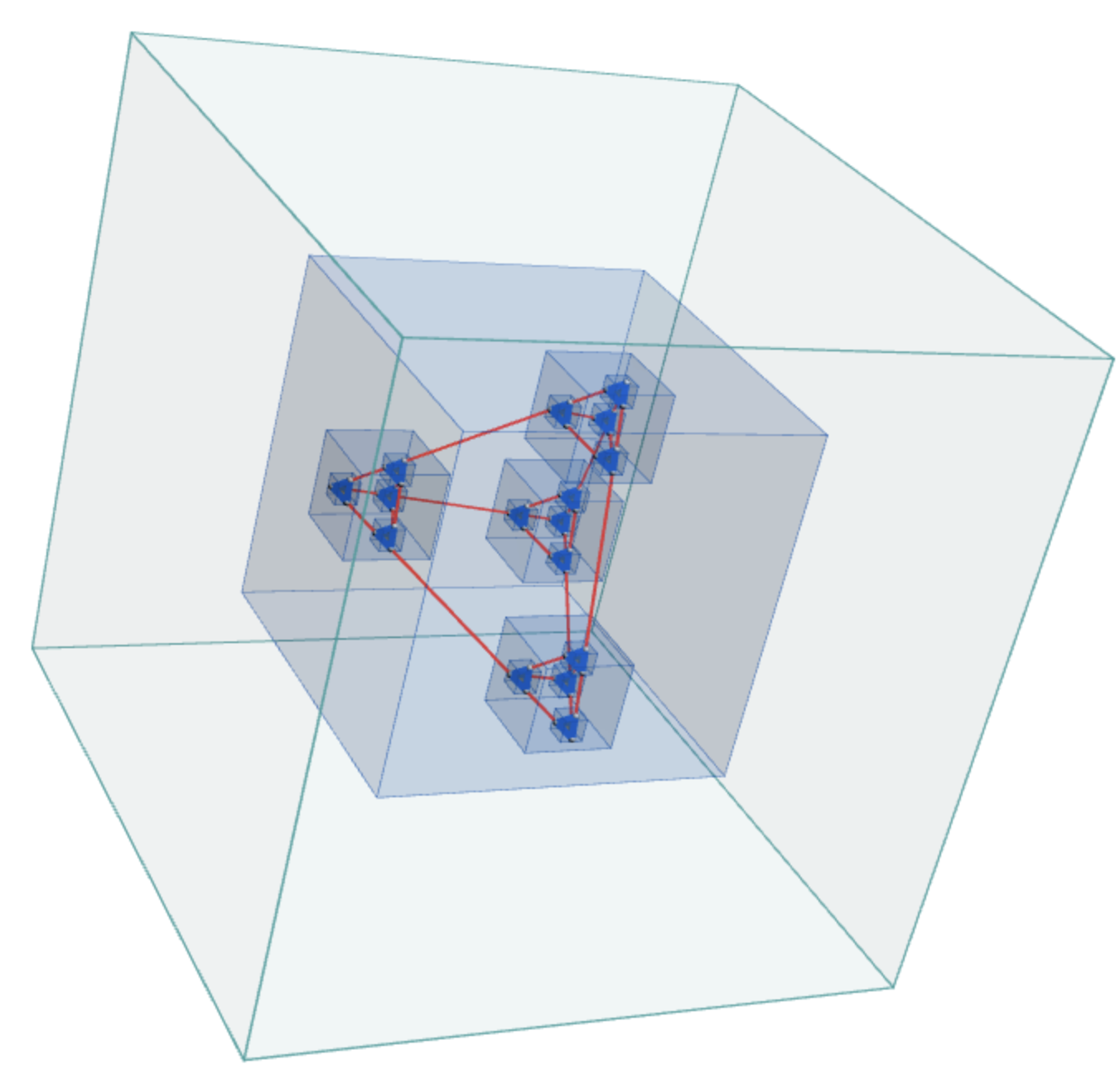
Finally, we can enclose each of the tetrahedrons in a cube whose faces are transversal to the edges of the $1$ -skeletons. Indeed, the edges of the $1$ -skeleton comprise six different directions. Consequently, this requirement is the complement of a finite number of linear conditions and thus achievable. By enlarging the cubes slightly we can suppose the edges intersect the faces of the cube in the interior of the faces and not on edges or vertices.

By iterating this $n$ times we can assume we are working with a knot embedded on the $1$ - skeleton of a graph constructed as above.

We now introduce a definition that will make our description easier to follow.

Definition 9.

We say a tetrahedron $\Delta$ , of any iteration, is a smallest tetrahedron if

\emptyset\neq K\cap\Delta\subseteq(1-\text{skeleton of }\Delta).

In other words, of $\Delta$ , $K$ only uses its edges but never goes into the faces or interior.

We say a cube is a smallest cube if the biggest tetrahedron in its interior is a smallest tetrahedron.

Our last enhancement of our construction is to surround each vertex of the smallest tetrahedrons with a cube, parallel to all the cubes in our construction, disjoint among themselves and within the interior of the corresponding smallest cube.

Definition 10.

The cubes just constructed will be called vertex cubes.

4.2 The thickening of the vertices

Definition 6 of sphere decomposition involves a thickened embedding of $K$ . So far, we have only modified the $1$ -skeleton so that we are able to surround individual tetrahedrons in their own cubes as shown in figure 7. In this subsection we briefly discuss the vertices. As we shall see, we can thicken them with a small polyhedron as long as we have control of a particular subtlety that arises.

In the definition of sphere weight, we intersect the sphere $S$ with the thickened graph and count the connected components of the intersection. In the sphere decomposition we will build, all our spheres will be rectangular prisms whose faces are parallel to three orthogonal fixed planes. Consequently, we must understand how these families of planes intersect the thickened vertex

As we sweep with planes that pass through the vertex, as if they were scanning the zone the vertex lies in, what we desire is to obtain a count of how the edges grow and merge into a corner. However, we must also count the intersection of this sweeping plane with the sphere.

As we can see in figure 8, as we approach the vertex we intersect the sphere in a component that is artificial. It will eventually merge with the other points on the edges but, nevertheless, made the weight of the sphere (i.e. the sweeping plane) to grow. We cannot disappear this problem by choosing a small enough sphere or similar. These intersections are features of the round shape of the sphere (or the polyhedron). Consequently, to prove an upper bound on the spherewidth, we must guarantee our thickening does not make the weight grow artificially beyond our desired bound. We will prove in due time our sphere decomposition satisfies this.

Remark 7.

There is another possibility to handle this. We can design an appropriate piece so that, if we are careful with our construction of the tree decomposition, these artificial intersections do not happen. This leads to the theory of separating polygons, Dirichlet - Voronoi cells, etc.

Thus, there is a dichotomy: we can let them happen but with bounded contribution or we can eliminate them. Once we make this choice, we design the tree decomposition.

With this in mind, we put around each vertex of each smallest pyramid a thickening polyhedron contained in the vertex cube. At the last step of our calculation, we will reduce the size of each of these polyhedrons. We will see this doesn’t create conflict with any construction as we can put the correct ones from the very start once we know what extra property we require from them.

4.3 The subdivision

Once the above has been carried out we have the following data:

1.

A finite number of cubes arranged in the way described above. Each cube, except for the vertex cubes, has inside exactly 4 smaller cubes arranged as in figure 7(a).
2.

A cycle through some of the edges described above that knots as $K$ .

All the above information induces a subdivision into closed sets of $\mathbb{S}^{3}$ as follows:

The exterior

The closure of the exterior of the largest cube. This includes the point at infinity and is homeomorphic to a ball $\mathbb{B}^{3}$ .

The intermediate regions

Each cube $C$ , except for the vertex cubes, has up four disjoint cubes inside of it.

However, we shall only consider the cubes if the knot $K$ intersects it. Otherwise we do not collocate a cube there as we can remove that part of the skeleton without altering the knot embedding. If $C_{1},...,C_{k}$ are the remaining cubes, the closed set is

\overline{C-(C_{1}\cup\cdots\cup C_{k})}.

The vertex cubes

A finite number of vertex cubes that inside hold a thickened vertex that belongs to the path traced by $K$ . The other vertex cubes, that were not visited, and the edges connecting to them are erased, without modifying the path $K$ traces.

Example 1.

A generic intermediate region can be seen in figure 9.

Notice that, except for cubes that surround one of the corners of the original pyramids, every cube has a way to go out of $C$ because it must connect to some other pyramid in another intermediate region. This possible way outs are marked by the purple vertices and dashed lines.

From each interior cube there is only one connecting line outside. The three dashed lines presented for each interior cube show the possibilities for this connecting line. Which one it is depends on the location of the cube within the pyramid. Furthermore, the cubes that contain the corners of the initial tetrahedron do not have any connecting lines to the exterior of the surrounding cube.

On the other hand, in figure 9, we see that the yellow points on a cube are potential intersections of the knot with the surface of these interior cubes. It is possible a knot intersects in all of them, some of them, or that it uses none in case that cube is not visited. In the latter case, we have agreed to not put any cube and remove all the part of the $1$ -skeleton that would be there.

We emphasize that figure 9 continues to hold for the smallest regions, where these cubes are the vertex cubes (i.e. the interior cubes we have thickened vertices as opposed to another tetrahedron)

The strategy we will follow is the next one: for each one of these closed sets $\mathcal{C}$ we will construct a continuous map $f_{\mathcal{C}}\mathrel{\mathop{\mathchar 58\relax}}\mathcal{C}\longrightarrow\mathcal{T}_{\mathcal{C}}$ , where $\mathcal{T}_{\mathcal{C}}$ is a trivalent tree. We will then glue the trees $\mathcal{T}_{\mathcal{C}}$ to form a trivalent tree $\mathcal{T}$ . Finally, the gluing lemma will imply the corresponding map $f\mathrel{\mathop{\mathchar 58\relax}}\mathbb{S}^{3}\longrightarrow\mathcal{T}$ is continuous. Once we have done this, we shall verify $f$ is a sphere decomposition.

The following is the fact which makes the whole computation work.

Proposition 2.

Let $C$ be any of the cubes of the above described subdivision.

1.

The intersection $\partial C\cap K$ has at most four connected components of $K$ (all them points).
2.

The intersection $C\cap K$ has at most two connected components.

Proof.

By construction, to cross $\partial C$ , the knot must go through one of the dashed lines towards the outside. However, per interior cube there is at most one way out, as each pyramid connects to at most one other pyramid at each of its vertices. As there are four vertices, this number is at most four. This proves $1$ .

If $C$ is the outer surrounding cube this is obvious as the knot is connected. For other cubes, if the knot visits the given cube then, it must go out of it. As we have establish to go in or out one must visit one of the four points on $\partial C$ . Hence, there can be at most two pairings, of these four vertices, as entry-exit pairs. This proves $2$ . ∎

4.4 The tree for an intermediate region

In this subsection we construct a trivalent tree associated to each intermediate region $\mathcal{C}$ .

Lemma 1.

Let $\mathcal{C}$ be an intermediate region. There exists a trivalent tree $\mathcal{T}_{\mathcal{C}}$ and a continuous map $f_{\mathcal{C}}\mathrel{\mathop{\mathchar 58\relax}}\mathcal{C}\longrightarrow\mathcal{T}_{\mathcal{C}}$ that satisfies the following properties:

1.

For each vertex $x$ that is not a leaf, the preimage $f^{-1}(x)$ is a double bubble transversal to $K\cap\mathcal{C}$ .
2.

For each point $x$ that is not a vertex, the preimage $f^{-1}(x)$ is a sphere transversal to $K$ .
3.

The tree $\mathcal{T}_{\mathcal{C}}$ has a single root corresponding to its surrounding cube and one leaf for each one of its interior cubes.
4.

Let $x_{1},x_{2}\in\mathcal{T}$ two points that are not trivalent vertices. If they are in the same edge, then

$w(f^{-1}(x_{1}),K)=w(f^{-1}(x_{2}),K).$

Proof.

For concreteness, let us call the interior cubes $A,B,C$ and $D$ and the surrounding cube $E$ . The technique is extremely simple: we will merge the cubes progressively. The process to do it will be to collocate the two chosen prisms to be merged into a third one and then invoke proposition 1.

We begin with an observation. We can assume that our initial configuration, that then gets repeated at each iteration, has all of its interior cubes small enough so that no plane parallel to the faces of the cubes intersects two of the interior cubes simultaneously. In particular, in between any two cubes there is a separating plane in every direction parallel to the faces of the cube

This is because we can pick the scalar factor of the Sierpinski tetrahedron to be as small as needed. Hence, the cube around it becomes as small as required to give the above separations. We only need this to work for one iteration. For all subsequent iterations we use the same configuration, under the appropriate scaling.

This allow us to guarantee that all prisms we will construct do not intersect more cubes than those they surround. This also implies that all edges they intersect have one of their endpoints in one of the prisms they surround. Indeed, if both endpoints were on the other side of the separating plane, by convexity of half-spaces, all the edge is.

We will “merge” $A$ and $C$ . To do this, we put them inside a common prism $R$ , whose faces are parallel to the faces of the cubes.Then we choose the membrane between them in such a way that it only intersects the edge between $A$ and $C$ (this intersection is unavoidable). Then we repeat this construction with $R$ and $D$ , and call the surrounding prism $Q$ . We conclude by repeating this with $Q$ and $B$ , and call the surrounding prism $U$ . We can see this in figure 10.

Once more, we emphasize this construction is possible because we can guarantee the edges of the merging prisms are far away from the faces of the other cubes that are not being merged. We can see this entire decomposition in figure 11.

Let us now discuss the construction of the map $f_{\mathcal{C}}$ . For concreteness, let us give the list of mergings we have done.

1.

$A$ and $C$ merge to $R$ ,
2.

$R$ and $D$ merge to $Q$ ,
3.

$Q$ and $B$ merge to $U$ ,

Notice that $U$ is a prism parallel to the surrounding cube $E$ and with all the cubes $A,B,C,D$ in its interior.

Pick any of the above steps, where two prisms are being merged. Let us call them $X$ and $Y$ . Let us call $Z$ the rectangular prism that is being used to merge them (for example, if $X=R$ and $Y=D$ , then $Z=Q$ ). Its faces are parallel to those of $X$ and $Y$ and that strictly contains them in its interior. Then divide $Z$ by a parallel subface (i.e. the “membrane”), disjoint from $X$ and $Y$ , into two smaller rectangles $Z_{X}$ and $Z_{Y}$ such that $X\subset Z_{X}$ and $Y\subset Z_{Y}$ . Notice that we can always pick the membrane so that it only intersects the edges between $X$ and $Y$ but no others.

Define

	$\displaystyle\mathcal{S}_{X,Z_{X}}$	$\displaystyle\mathrel{\mathop{\mathchar 58\relax}}=\overline{Z_{X}-X},$
	$\displaystyle\mathcal{S}_{Y,Z_{Y}}$	$\displaystyle\mathrel{\mathop{\mathchar 58\relax}}=\overline{Z_{Y}-Y}.$

By proposition 1 there exist maps

	$\displaystyle\Phi_{X}\mathrel{\mathop{\mathchar 58\relax}}\mathcal{S}_{X,Z_{X}}\longrightarrow[a,b],$
	$\displaystyle\Phi_{Y}\mathrel{\mathop{\mathchar 58\relax}}\mathcal{S}_{Y,Z_{Y}}\longrightarrow[c,d],$

such that the level sets are rectangular prisms with faces parallels to those of $X$ and $Y$ . We now identify $b$ and $d$ to create a path $P$ whose vertices are $a,b=d,c$ . We define

\Phi_{XY}\mathrel{\mathop{\mathchar 58\relax}}\mathcal{S}_{X,Z_{X}}\cup\mathcal{S}_{Y,Z_{Y}}\longrightarrow P,

as $\Phi_{X}$ on $\mathcal{S}_{X,Z_{X}}$ and as $\Phi_{Y}$ on $\mathcal{S}_{Y,Z_{Y}}$ . The gluing lemma implies this is a well-defined continuous map as $\Phi_{X}$ and $\Phi_{Y}$ coincide on the membrane (whose image is $b=d$ ). Notice that

\mathcal{S}_{X,Y}\mathrel{\mathop{\mathchar 58\relax}}=\overline{Z-X-Y}=\mathcal{S}_{X,Z_{X}}\cup\mathcal{S}_{Y,Z_{Y}}.

Consequently, we have built a map

\Phi_{XY}\mathrel{\mathop{\mathchar 58\relax}}\mathcal{S}_{X,Y}\longrightarrow P,

By construction, the following holds

	$\displaystyle\Phi^{-1}_{XY}(a)$	$\displaystyle=X,$
	$\displaystyle\Phi^{-1}_{XY}(c)$	$\displaystyle=Y,$
	$\displaystyle\Phi^{-1}_{XY}(b=d)$	$\displaystyle=Z_{X}\cup Z_{Y}.$

Notice that this last preimage is a double bubble, as it is $Z$ together with the membrane.

Let us construct a map corresponding to $U$ and $E$ . By proposition 1, there exists

\Phi_{U,E}\mathrel{\mathop{\mathchar 58\relax}}\mathcal{S}_{U,E}\longrightarrow[e,f],

such that its level sets are prisms with faces parallel to those of $U$ and $E$ . In here we have defined

\mathcal{S}_{U,E}=\overline{E-U}.

We now have four maps $\Phi_{A,C}$ , $\Phi_{R,D}$ , $\Phi_{Q,B}$ and $\Phi_{U,E}$ . Each goes to a different path. Notice that we can normalize notation as follows:

	$\displaystyle\Phi_{A,C}\mathrel{\mathop{\mathchar 58\relax}}$	$\displaystyle\mathcal{S}_{A,C}\longrightarrow[v_{A},v_{C}],$
	$\displaystyle\Phi_{R,D}\mathrel{\mathop{\mathchar 58\relax}}$	$\displaystyle\mathcal{S}_{R,D}\longrightarrow[v_{R},v_{D}],$
	$\displaystyle\Phi_{Q,B}\mathrel{\mathop{\mathchar 58\relax}}$	$\displaystyle\mathcal{S}_{Q,B}\longrightarrow[v_{Q},v_{B}],$
	$\displaystyle\Phi_{U,E}\mathrel{\mathop{\mathchar 58\relax}}$	$\displaystyle\mathcal{S}_{U,E}\longrightarrow[v_{U},v_{E}].$

For the first three maps, the edge on the codomain has an interior vertex whose preimage is a double bubble. Respectively, we call this interior vertex $w_{R},w_{Q},w_{U}$ . The corresponding double bubble is the one whose exterior prism is $R,Q$ and $U$ , respectively.

We intend to use the gluing map to construct out of these four maps a map on the intermediate region $\mathcal{C}$ . We have

\mathcal{C}=\overline{E-(A\cup B\cup C\cup D)}=\mathcal{S}_{A,C}\cup\mathcal{S}_{R,D}\cup\mathcal{S}_{Q,B}\cup\mathcal{S}_{U,E}.

(1)

Consequently, if we define appropriate maps that coincide in the intersections, the gluing lemma concludes the task. The target codomain will be a trivalent tree $\mathcal{T}_{\mathcal{C}}$ . We construct it as an identification space, constructed from the edges $[v_{A},v_{C}]$ , $[v_{R},v_{D}]$ , $[v_{Q},v_{B}]$ and $[v_{U},v_{E}]$ , by the identifications

w_{R}\sim v_{R},\;w_{Q}\sim v_{Q},\;w_{U}\sim v_{U}.

Notice that this is indeed a trivalent tree. Its leaves are $v_{A},v_{B},v_{C}$ , $v_{D}$ and $v_{E}$ and its trivalent vertices are $w_{R}=v_{R}$ , $w_{Q}=v_{Q}$ and $w_{U}=v_{U}$ . This verifies property $3$ about $\mathcal{T}_{\mathcal{C}}$ .

The nonempty double intersections among the closed sets of equation (1) are

	$\displaystyle\mathcal{S}_{A,C}\cap\mathcal{S}_{R,D}$	$\displaystyle=R,$
	$\displaystyle\mathcal{S}_{R,D}\cap\mathcal{S}_{Q,B}$	$\displaystyle=Q,$
	$\displaystyle\mathcal{S}_{Q,B}\cap\mathcal{S}_{U,E}$	$\displaystyle=U.$

Notice that the membranes, other than their edges, are not part of the intersections. The corresponding maps coincide in these intersections because their images are the identified vertices. Hence, by the gluing lemma, there is a continuous map

f_{\mathcal{C}}\mathrel{\mathop{\mathchar 58\relax}}\mathcal{C}\longrightarrow\mathcal{T}_{\mathcal{C}}

We claim that this map satisfies all the desired properties $1,2$ and $4$ . The trivalent vertices $v_{R},v_{Q},v_{U}$ satisfy

	$\displaystyle f_{\mathcal{C}}^{-1}(v_{R})$	$\displaystyle=\Phi_{A,C}^{-1}(v_{R})=R_{A}\cup R_{C},$
	$\displaystyle f_{\mathcal{C}}^{-1}(v_{Q})$	$\displaystyle=\Phi_{R,D}^{-1}(v_{Q})=Q_{R}\cup Q_{D},$
	$\displaystyle f_{\mathcal{C}}^{-1}(v_{U})$	$\displaystyle=\Phi_{Q,B}^{-1}(v_{U})=U_{Q}\cup U_{B},$

each of which is a double bubble. Notice this double bubble never intersects vertices, as there are none in $\mathcal{C}$ . Furthermore, by construction the intersections with the edges is transversal. This proves property $1$ . (Notice that $R_{A}$ , $R_{C}$ , etc. are what we called $Z_{X}$ and $Z_{Y}$ when we constructed these maps above.)

Property $2$ follows from proposition 1, because these preimages are precisely the preimages of interpolations. These preimages are prisms whose faces are parallel to those of the cubes. As we know, by construction, the edges of the $1$ -skeleton are never parallel to these faces. Furthermore, also by construction, if one of these spheres intersects an edge, then it has a point of the edge inside of it. Therefore, all intersections are transversal (as opposed to tangent).

Finally, to prove property $4$ we recall proposition 2. We already proved that for each interior points $x$ , $f^{-1}_{\mathcal{C}}(x)$ is a rectangular prism with faces parallel to those of the cubes. This also holds for the leaves themselves, where we recover $\partial A,\partial B,\partial C$ and $\partial D$ as preimages. However, we know more: this prism is a level set of one of the four glued maps. Hence, in order to prove this property, we will trace these maps in order.

Recall that $\mathcal{C}\cap K$ are the edges between the cubes and those segments from $A,B,C$ and $D$ that go out of $E$ . Because the intersection is transversal, each of these segments intersects $f^{-1}_{\mathcal{C}}(x)$ in a finite number of points. Suppose that $f^{-1}_{\mathcal{C}}(x)$ interpolates between $X$ and $Z_{X}$ . We agree to take $Z_{X}=E$ if $X=U$ . Notice that for every $x$ , interior to the edges, we can find an $X$ that satisfies this.

Let $p\in f^{-1}_{\mathcal{C}}(x)\cap K$ . Consequently,

p\in K\cap\mathcal{S}_{X,Z_{X}}.

This intersection consists of closed intervals. By construction, all of these intervals have at least one of their endpoints on $\partial X$ . Thus $p$ is connected to $\partial X$ through one of these edges. Hence, we have a correspondence

f^{-1}_{\mathcal{C}}(x)\cap K\longrightarrow\partial X\cap K.

We claim this correspondence is bijective. If $p_{1}$ and $p_{2}$ correspond to the same point, then $p_{1}p_{2}$ would be part of the given segment. However, $f^{-1}_{\mathcal{C}}(x)$ is a rectangular prism with one of the endpoints of this segment inside. As this segment is transversal to the faces of the prism, they can only intersect it in at most one point. Hence $p_{1}=p_{2}$ . It is surjective for a similar reason. Given a point $p\in K\cap\partial X$ , it must be part of a unique edge of $K$ . The other endpoint of this edge lies on a vertex within another cube. By construction $Z_{X}$ only contains the cubes inside of $X$ (possibly $X$ itself). Hence, this edge has a point inside $f^{-1}_{\mathcal{C}}(x)$ and one outside. It must therefore intersect it at some point.

The count of these points is, by definition, the weight of the spheres. Hence, we have proven is

w(f^{-1}(x),K)=w(\partial X,K).

(2)

If $x_{1}$ and $x_{2}$ belong to the same edge, but are not trivalent vertices, they were not identified in the process of creating $\mathcal{T}$ with another point. Hence, ther exists $X,Y$ such that

x_{1},x_{2}\in[v_{X},v_{Y}]

In the case where there is an identification point between $v_{X}$ and $v_{Y}$ , we must have $x_{1}$ and $x_{2}$ are on the same side of it. Otherwise they would be in different edge. This implies, by construction, that, $f^{-1}(x_{1})$ and $f^{-1}(x_{2})$ are interpolations between $X$ and $Z_{X}$ for the same $X$ . Equation (2) implies

w(f^{-1}(x_{1}),K)=w(\partial X,K)=w(f^{-1}(x_{2}),K),

as desired. This concludes the proof. ∎

Proposition 3.

Let $\mathcal{C}$ be an intermediate region and $f_{\mathcal{C}}\mathrel{\mathop{\mathchar 58\relax}}\mathcal{C}\longrightarrow\mathcal{T}$ the map constructed in lemma 1. Then for all $x\in\mathcal{T}$ that is not a trivalent vertex,

w(f^{-1}(x),K)\leq 6.

Proof.

For an interior cube $V$ (i.e. $V$ is one of $A,B,C$ or $D$ ) define

\delta_{V}=\begin{cases}1,&\text{if }K\text{ enters or exits through }V,\\ 0,&\text{otherwise }.\end{cases}

Similarly, for two interior cubes $V$ and $W$ define

\delta_{VW}=\begin{cases}1,&\text{if }K\text{ uses }VW,\\ 0,&\text{otherwise }.\end{cases}

Then we have

w(A,K)=\delta_{A}+\delta_{AB}+\delta_{AC}+\delta_{AD}.

Similar for the other vertices. When we merge two cubes, say $A$ and $B$ , in a third prism $R$ the weight calculation is

w(R,K)=w(A,K)+w(B,K)-2\delta_{AB}=\delta_{A}+\delta_{B}+\delta_{AC}+\delta_{AD}+\delta_{BC}+\delta_{BD}.

Similarly, merging now $R$ and $C$ into a prism $Q$ , we get

w(Q,K)=\delta_{A}+\delta_{B}++\delta_{C}+\delta_{AD}+\delta_{BD}+\delta_{CD}.

And finally, of course, for the surrounding region

\delta(E,K)=\delta_{A}+\delta_{B}+\delta_{C}+\delta_{D}.

As all of these calculations at most sum six terms, each of which is a $0$ or a $1$ , the bound of $6$ follows. ∎

Corollary 1.

Let $\mathcal{C}$ be an intermediate region and $f_{\mathcal{C}}\mathrel{\mathop{\mathchar 58\relax}}\mathcal{C}\longrightarrow\mathcal{T}$ the map constructed in lemma 1.

1.

Suppose there is one interior cube with one of its adjacent edges in $\mathcal{C}$ not used by the knot, then for all $x\in\mathcal{T}_{\mathcal{C}}$ that are not trivalent vertices we have

$w(f^{-1}_{\mathcal{C}}(x),K)\leq 4.$
2.

On the other hand, if all edges are used in $\mathcal{C}$ , then for some $x\in\mathcal{T}_{\mathcal{C}}$ that is not a trivalent vertex, we have

$w(f^{-1}_{\mathcal{C}}(x),K)=6.$

Proof.

By proposition 2, interior cubes must have either $0$ , $2$ or $4$ points on their surfaces. Therefore, the initial weights are even.

The calculation of the successive weights implies they are also even, as you subtract twice the number of shared edges. In particular, if one can guarantee the sum is not six, then it is at most four.

Only the two intermediate calculations, in the proof of proposition 3, can be six. Concretely, with the notation of that proposition,

	$\displaystyle w(R,K)$	$\displaystyle=\delta_{A}+\delta_{B}+\delta_{AC}+\delta_{AD}+\delta_{BC}+\delta_{BD}$
	$\displaystyle w(Q,K)$	$\displaystyle=\delta_{A}+\delta_{B}++\delta_{C}+\delta_{AD}+\delta_{BD}+\delta_{CD}$

Bot of this sums share $\delta_{A}$ and $\delta_{AD}$ . Thus, declaring the cube in the hypothesis to be $A$ we see $\delta_{A}$ or $\delta_{AD}=0$ (where, in the latter case, $D$ is the vertex on the other end of the missing edge.)

We conclude these sums cannot be six, hence they are at most four. By property $4$ of lemma 1, all the weights reduce the this count. This proves $1$ .

On the other hand, if such an intermediate region exists, then the count for $w(R,K)=6$ , because

\delta_{A}=\delta_{B}=\delta_{AC}=\delta_{AD}=\delta_{BC}=\delta_{BD}=1.

The result follows. ∎

4.5 The vertex cubes

The results of the previous subsection have taken care of almost all the regions where we need to construct the sphere decomposition. We are missing the exterior of the largest surrounding cube and the vertex cubes. We will return to the former in the proof of the main theorem.

Lemma 2.

Let $C$ be a vertex cube around the vertex $V$ . There exists a thickening of $V$ to a polyhedron $\mathcal{P}$ and a map $f_{C}\mathrel{\mathop{\mathchar 58\relax}}C\longrightarrow[0,1]$ such that

1.

For each $0<u\leq 1$ , the level set $f^{-1}(u)$ is a rectangular prism transversal or finitely tangent to $K$ thickened with $\mathcal{P}$ .
2.

For each $0<u\leq 1$ , we have

$w(f^{-1}_{C}(u),K)\leq 3,$

where this weight is computed with respect to the thickened graph $K\cap C$ using $\mathcal{P}$ .
3.

$f^{-1}_{C}(0)$ is a point disjoint from $K$ .

Proof.

The vertex cubes have, by definition, the vertices of the $1$ -skeleton that have been visited by the knot. Consequently, these vertices have degree $2$ .

For any interior point $p$ of $C$ , we can create the linear homotopy from $C$ to $p$ :

H(x,u)=(1-u)p+ux,\;\;0\leq u\leq 1.

(3)

This generic homotopy divides the cube into six different pyramids whose bases are parallel to a face of the cube. As long as $p$ is not collinear with $V$ and a point on the edges of the cube, the vertex $V$ will be in the interior of one of these pyramids. This is an open condition and can always be achieved. We will assume we have fixed such a point $p$ and we will call it $p_{V}$ . We can further assume that $p_{V}$ is not on $K$ . We will denote the pyramid it lies by $\Delta$ .

For each $0<u\leq 1$ , the level set

C_{u}\mathrel{\mathop{\mathchar 58\relax}}=\{H(x,u)\mid x\in C\},

is also a cube homothetic to $C$ , from $p_{V}$ . In particular, because it has $V$ in its interior, and the two edges incident at $V$ intersect $C$ , they must also intersect $C_{t}$ at two points.

Finally, because $V$ lies in the interior of $\Delta$ , we can put a small convex polyhedron $\mathcal{P}$ around $P$ that lies in the interior of $\Delta$ . We further assume all the faces of $\mathcal{P}$ are transversal to the edges of the knot, which is to say, to the sides of the $1$ -skeleton. We also assume its faces are transversal to the faces of the cubes. Together these are a finite number of linear conditions, so such convex polyhedron exists. We claim that if we thicken $V$ with this $\mathcal{P}$ , the result will follow.

Proposition 1 applied to $p_{V}$ and $C$ implies the existence of a map

f_{C}\mathrel{\mathop{\mathchar 58\relax}}C\longrightarrow[0,1].

The level sets of these maps are the $C_{u}$ defined above (this is part of the proof of proposition 1. We refer the reader to it.)

For the intersection with the edges, Property 1 follows from the corresponding property of proposition 1. For the intersection with the thickened vertex, we do as follows. The thickened vertex $\mathcal{P}$ lies strictly inside $\Delta$ . Hence, for a fixed level set, $\mathcal{P}$ can only intersect its face parallel to the base of $\Delta$ . This face lies on a plane parallel to the faces of the cube. Consequently, the intersection will be a single component. Indeed, a plane and a convex polyhedron intersect in a single component, which is the boundary of the convex polygon that the plane cuts of the solid polyhedron. If this intersection is a single point, then the intersection is finitely tangent. On the other hand, if the intersection is a proper polygon, then on each face of $\mathcal{P}$ , the intersection is between two non-parallel planes. Hence, it is transversal. This concludes the proof of property $1$ .

To see the validity of property $2$ , notice that the thickened graph $K\cap\mathcal{C}$ has three pieces: $\mathcal{P}$ and the two edges adjacent to $V$ without their segment interior to $\mathcal{P}$ .

The weight is, by definition, the number of connected components of the intersection. These intersections can be of two kinds: $f_{C}^{-1}(u)$ intersects only the edges or it intersects $\mathcal{P}$ and the edges. Each edge, being a straight segment transversal to all the faces of the level set, can only intersect it at one point. Thus, the edges contribute to the weight at most $2$ . We justified above that the only face of the cube that intersects $\mathcal{P}$ does it in at most one component (which might be an artifical intersection). We conclude that, in any case, the number of connected components in the intersection are at most $3$ .

Finally, property $3$ is true because $f_{C}^{-1}(0)=p_{V}$ which by construction is the center of the homotopy and is disjoint from $K$ thickened by $\mathcal{P}$

This concludes the proof. ∎

Remark 8.

If we were uncareful and we just make an homotopy (or something similar) but we do not control where are the intersections with $\mathcal{P}$ we could land in the situation that all the faces intersect $\mathcal{P}$ and, on top, they intersect the edges outside. This would give a count of $8$ , which would make our bound grow unnecessarily.

4.6 The main theorem

We have now done all the required work. We can finally prove

Theorem 1.

Let $K$ be a knot that can be embedded in a finite iteration of the Sierpinski tetrahedron. Then $K$ admits a sphere decomposition of weight at most $6$ .

Proof.

Let $\mathcal{C}_{1},...,\mathcal{C}_{m}$ be all the intermediate regions. Let $E$ be the exterior cube. Let $P_{1},...,P_{k}$ be the vertex cubes used in the construction. In other words, inside of them are the vertices of the smallest tetrahedrons visited by the knot. Without loss of generality assume that $\mathcal{C}_{1}$ is the intermediate region whose surrounding cube is $E$ itself.

We can define an homotopy $H\mathrel{\mathop{\mathchar 58\relax}}E\times[0,\infty)\longrightarrow\overline{\mathbb{S}^{3}-E-\{\infty\}}$ by

H(e,u)=ue

At a fixed time $u_{0}$ , the image of $e\longrightarrow H(e,u_{0})$ is a cube $E_{u_{0}}$ with sides parallel to $E$ . Consequently, we have a map

f_{E}\mathrel{\mathop{\mathchar 58\relax}}\overline{\mathbb{S}^{3}-E}\longrightarrow[1,\infty],

given by

f_{E}(x)=t

if $x\in E_{t}$ and $f_{E}(\infty)=\infty$ . We shall call $\infty$ the root of this tree (which is an edge) and call it $\mathcal{T}_{\infty}$ . This map is continuous and the proof is the same as that of proposition 1.

In this way, we have a family of continuous maps $f_{E},f_{C_{1}},...,f_{C_{m}}$ , $f_{P_{1}},...,f_{P_{k}}$ . For the intermediate regions, the maps $f_{C_{j}}$ are the ones constructed in lemma 1. For the vertex cubes the maps are constructed in lemma 2.

Suppose $\mathcal{C}$ is an intermediate region and $X_{1},...,X_{k}$ are the contiguous regions it surrounds. We know $1\leq k\leq 4$ . Each $X_{i}$ is a cube, possibly a vertex cube.

By construction, the tree $\mathcal{T}_{\mathcal{C}}$ has a vertex labeled after each $X_{i}$ . In the same way, the trees $\mathcal{T}_{X_{i}}$ has its root labeled after $X_{i}$ . Thus, if we identify the leaf associated to $X_{i}$ in $\mathcal{T}_{\mathcal{C}}$ with the root of $\mathcal{T}_{X_{i}}$ , for each $1\leq i\leq k$ , we obtain a new tree $\mathcal{T}_{0}$ . The vertices where the gluing happened have degree two because each glued tree contributed one edge. In $\mathcal{T}_{0}$ we now consider this gluing point as part of the edge and not a vertex.

Notice that

\mathcal{C}\cup X_{1}\cup\cdots\cup X_{k}

is a finite union of closed sets and the nonempty intersections among them are the exterior boundaries of $X_{1},...,X_{k}$ . Consequently, we can define

f_{0}\mathrel{\mathop{\mathchar 58\relax}}\mathcal{C}\cup X_{1}\cup\cdots\cup X_{k}\longrightarrow\mathcal{T}_{0},

as $f_{\mathcal{C}}$ in ${\mathcal{C}}$ and $f_{X_{i}}$ in $X_{i}$ . The gluing lemma implies this map is continuous. Notice that under this map the preimage of the gluing points are precisely the boundaries of $X_{i}$ , which are topological spheres.

Let us summarize what have we done. For each intermediate region, we have created a new map that extends $f_{\mathcal{C}}$ into the interiors of the regions it surrounds. We have done this in such a way that the codomain is a tree built out of the trees we already had. We can now proceed inductively from the first intermediate region towards the vertex cubes. Indeed, our previous construction guarantees we can extend the map up to $C_{1}\cup X_{1}\cdots\cup X_{k}$ . If all of these $X_{1},...,X_{k}$ are vertex cubes then we have

E=\mathcal{C}_{1}\cup X_{1}\cup\cdots\cup X_{k},

(4)

and we have built a map in all of $E$ . If not then we repeat this argument in each of the $X_{i}$ that is an intermediate region. Once more the gluing lemma guarantees that the function we already have will glue continuously onto the tree formed by identifying the leaf associated to $X_{i}$ with the corresponding root. This process must finish because there is a finite number of regions.

Hence, we have a map $f_{1}\mathrel{\mathop{\mathchar 58\relax}}E\longrightarrow\mathcal{T}_{1}$ that is built by successively using the gluing lemma to attach together all the $f_{C_{1}},...,f_{C_{m}}$ , $f_{P_{1}},...,f_{P_{k}}$ . Finally, we apply the gluing lemma one last time to glue $f_{1}$ and $f_{E}$ along the boundary of $E$ , which is a cube, to produce a map $f\mathrel{\mathop{\mathchar 58\relax}}\mathbb{S}^{3}\longrightarrow\mathcal{T}$ . The tree $\mathcal{T}$ is obtained by gluing the trees of $f_{1}$ and $f_{E}$ at their corresponding vertex associated to $E$ , but this new point is not considered a vertex of the new tree. Our new tree has as root $\infty$ .

What now prove that $f\mathrel{\mathop{\mathchar 58\relax}}\mathbb{S}^{3}\longrightarrow\mathcal{T}$ is a sphere decomposition. We verify the properties one by one.

(SD 1) For all $x\in L(\mathcal{T})$ , $f^{-1}(x)$ is a point disjoint of $K$ : The trivalent tree $\mathcal{T}$ is formed by gluing the trees

\mathcal{T}_{\infty},\mathcal{T}_{\mathcal{C}_{1}},\mathcal{T}_{\mathcal{C}_{2}},...,\mathcal{T}_{\mathcal{C}_{m}},\mathcal{T}_{P_{1}},...,\mathcal{T}_{P_{k}}.

The leaves of $\mathcal{T}$ are those leaves of the above trees that were not glued. To do not be glued, the leave must be associated to a region that has no further region inside of them. This only occurs for $P_{1},...,P_{k}$ and $\overline{E^{c}}$ (whose inside is the region containing $\infty$ ). By construction, these trees are edges representing an homotopy from the region to a point. Neither of these touch $K$ . Indeed, the former do not by lemma 2. The latter, being $\infty$ , is not on $K$ . This proves the first property.

(SD 2)For all $x\in V(\mathcal{T})-L(\mathcal{T})$ , $f^{-1}(x)$ is a double bubble transverse to $K$ : The vertices in $V(\mathcal{T})-L(\mathcal{T})$ are the trivalent vertices. These vertices are not being identified to any other points, thus its preimage coincides with that of the corresponding map being glued. Furthermore, the only trees with trivalent vertices are those corresponding to $\mathcal{C}_{1},...,\mathcal{C}_{m}$ . The result now follows by lemma 1.

(SD 3) For all $x\in\mathcal{T}$ interior to an edge, $f^{-1}(x)$ is a sphere transverse or finitely tangent to $K$ : The vertices interior to an edge are of two sorts: those that are points of identification but not considered vertices and those that are interior to an edge and were not identified. The former ones correspond to the regions where two closed sets intersected. By construction, these are all surfaces of cubes transversal to $K$ . The latter points satisfy what we want by lemma 1 in the case of intermediate regions. For the case of $f_{\infty}$ , all these regions are surfaces of cubes. Finally, for the case of $f_{P_{k}}$ , this follows by lemma 2.

The three properties hold. Hence, $f$ is a sphere decomposition. To verify its width, we realize that each interior point has as a preimage the surface of a sphere of which we have already computed its weight.

We begin by interior points of the glued trees. For $f_{\infty}$ the weight is zero because they never intersect the knot. For every intermediate region, proposition 3, guarantees the intersection is at most $6$ . For the vertex cubes, lemma 2 implies the weight is bounded by $3$ .

For the interior points of $\mathcal{T}$ that were formed by identifying leaves of two other trees, notice that their preimage is precisely a boundary between an intermediate region and a contiguous one. For all of them, the intersection is at most $4$ , by proposition 2. Consequently, the spherewidth of $f_{\mathcal{C}}$ is bounded by $6$ .

This concludes the proof of the theorem. ∎

Remark 9.

In the course of the proof we have seen that the number of leaves of $\mathcal{T}$ is equal to the number of vertex cubes plus one, the root, associated to $\infty$ . The edges associated to the homotopies for the vertex cubes or the outer cube have weight at most $3$ . Their other vertex is one associated to the vertex cubes or, in the case of $\infty$ , to the surrounding cube $E$ . Consequently, the structure of the tree can be read from the rest of the information. In particular, in our further discussions we will ignore these edges as their information do not change our conclusions.

We finally have our desired result.

Theorem 2.

Proof.

In [5, Corollary 1.3] it is proven that

sw(T(p,q))\geq\dfrac{2}{3}\min\{p,q\}.

If $T(p,q)$ is in a finite iteration of the Sierpinski tetrahedron, theorem 1 implies

\dfrac{2}{3}\min\{p,q\}\leq 6.

In other words,

\min\{p,q\}\leq 9.

There are infinitely many torus knots not satisfying the above. This concludes the proof. ∎

5 An example with the Trefoil

In this section we will give an example for the trefoil $3_{1}$ . Part of our goal is to convince ourselves that the sphere decomposition, and hence the tree, can be read in an straightforward way from the diagram in the combinatorial representation.

5.1 Intermediate regions and the combinatorial representation

We recall that a combinatorial representation is a “map” of a finite iteration that allows us to see a finite iteration in two dimensions. It is constructed by flattening each iteration. This sequence can be seen in figure 12.

In particular, we can read the intermediate regions we used to construct our sphere decompositions, via the flattening of a single iteration. We see this in figure 13.

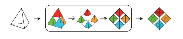
To construct the tree and count the weights of the spheres, what matter is to know how to connect different regions and the number of components on each intermediate sphere. By localizing in the corresponding zone of the combinatorial representation, this can be readily counted.

5.2 The example for the trefoil

In [1] we have found the trefoil in a finite iteration of the tetrahedron. This corresponds to the combinatorial representation show in figure 14.

In order to locate ourselves as we read, we will denote the different squares according to their position with respect to the north (N), south(S), east (E) and west (W) direction. For example, the first iteration has four pyramids corresponding to $N,S,E$ and $W$ . For another example, take the smallest tetrahedron, in figure 14, where the letter B is located. Its location is $NSS$ . We are in the third iteration so we need at most three coordinates. Finally, we shall call $F$ the exterior cube surrounding the whole tetrahedron.

Following our convention, the different intermediate regions, besides those in the smallest cubes, are:

1.

$F$ with interior cubes $N$ , $S$ and $W$ ,
2.

$N$ with interior cubes $NN$ , $NS$ , $NW$ , $NE$ .,
3.

$NW$ with interior cubes $NWN$ , $NW$ , $NWW$ and $NWE$ ,
4.

$NS$ with interior cubes $NSN$ , $NSW$ , $NSS$ and $NSE$ .

The smallest cubes of our configuration are: $W,S,NN,NE$ , $NWN$ , $NWS$ , $NWW$ , $NWE$ , $NSN$ , $NSW$ , $NSS$ and $NSE$ . Thus our final tree $\mathcal{T}$ will have $12$ leaves besides the root corresponding to $\infty$ . It will be constructed by gluing four trees, one per intermediate region. As per remark 9, we do not put the edges connecting to the leaves.

In order to see this more clearly, and be able to read our diagram easily, we have filled in the smallest cubes and highlighted the connections in figure 15. Each intermediate region is filled in with a different color. The connection edges within regions that are used by the knot appear in blue. Those that do not appear in red. Notice that $E$ does not appear because the knot does not visit that pyramid.

The way we will merge each of the intermediate regions, given in our above list, is as follows:

1.

We merge $N$ and $W$ . Then we merge with $S$ .
2.

We merge $NN$ with $NW$ . Then, we merge the result with $NS$ . Finally, we merge with $NE$ .
3.

We merge $NWW$ with $NWS$ . We then merge the result with $NWE$ . Finally, we merge with $NWN$ .
4.

We merge $NSW$ with $NSS$ . We then merge the result with $NSE$ . Finally, we merge with $NSN$ .

Finally we must count the number of components. We have repeatedly seen this is equivalent to counting how many points are on the surface, although the former count is half the latter one. This is done by inspection. We look at each smallest regions and count. For example $W$ has a single component. $S$ has a single component. On the other hand, $NSE$ has two components.

By 1, the weight of the spheres, does not change along edges. Thus, we only need to understand the components in tetrahedrons and not at intermediate stages.

We can now see the tree. We have them highlighted by intermediate region. Finally, the number registered is the number of components, thus the weight is double that number. We emphasize this is because, as we have seen in the course of the proof of theorem 1, all the involved intersections in the intermediate regions are transversal. Hence every connected component goes in and goes out at different points.

We conclude this is a sphere decomposition with width $6$ . Consequently $sw(3_{1})\leq 6$ .

Remark 10.

We did not need to construct the whole tree to deduce the spherewidth of $f$ . The intermediate regions at $NW$ and $NS$ use all edges among the interior cubes and exits. Hence, corollary 1 implies $sw(f)=6$ .

This doesn’t imply that $sw(3_{1})=6$ . As we will see, there are other sphere decompositions that bring the spherewidth lower.

6 Further Questions and Concluding Remarks

6.1 Pretzel Knots

In [1] we have proven that all Pretzel knots can be found in the finite iterations of the Sierpinski tetrahedron. Theorem 1 then implies its spherewidth is bounded by $6$ . This bound can be improved if one forgets about the tetrahedron.

Proposition 4.

Let $P(a_{1},...,a_{n})$ be a Pretzel knot, then

sw(P(a_{1},...,a_{n}))\leq 4.

(5)

Proof.

We will just describe the main steps as the details are exactly the same as those of our previous results. We will do it for pretzels of three strands for ease of explanation.

The proof consists of three main steps:

1.

Get the appropriate thickened embedding.
2.

Find the regions to be isolated so that the combinatorics outside of them are doable.
3.

Fill in with what happens in the isolated regions with their own computations.

For pretzel knots step $1$ can be done. We can assume all edges used are not parallel to any of the coordinate planes. We can thicken each vertex such that the weight in there, as we sweep, does not exceed $4$ . We will leave the details of this to the interested reader.

The regions that we will isolate are the individual tangles as well as the upper and lower strand joining the first and last tangles. To isolate them, we put around them solid prisms that are disjoint and that can be separated by planes in the $X$ and $Y$ directions. In this case we do not need the third direction because the membranes will only be parallel to two of the coordinate planes.

This step is analogous to our intermediate regions. We knew something happened on beyond the boundary, whether toward the exterior cube or toward the vertex cubes. However, that was unnecessary for the construction of the sphere decomposition in this region and for the calculations of the weights in there.

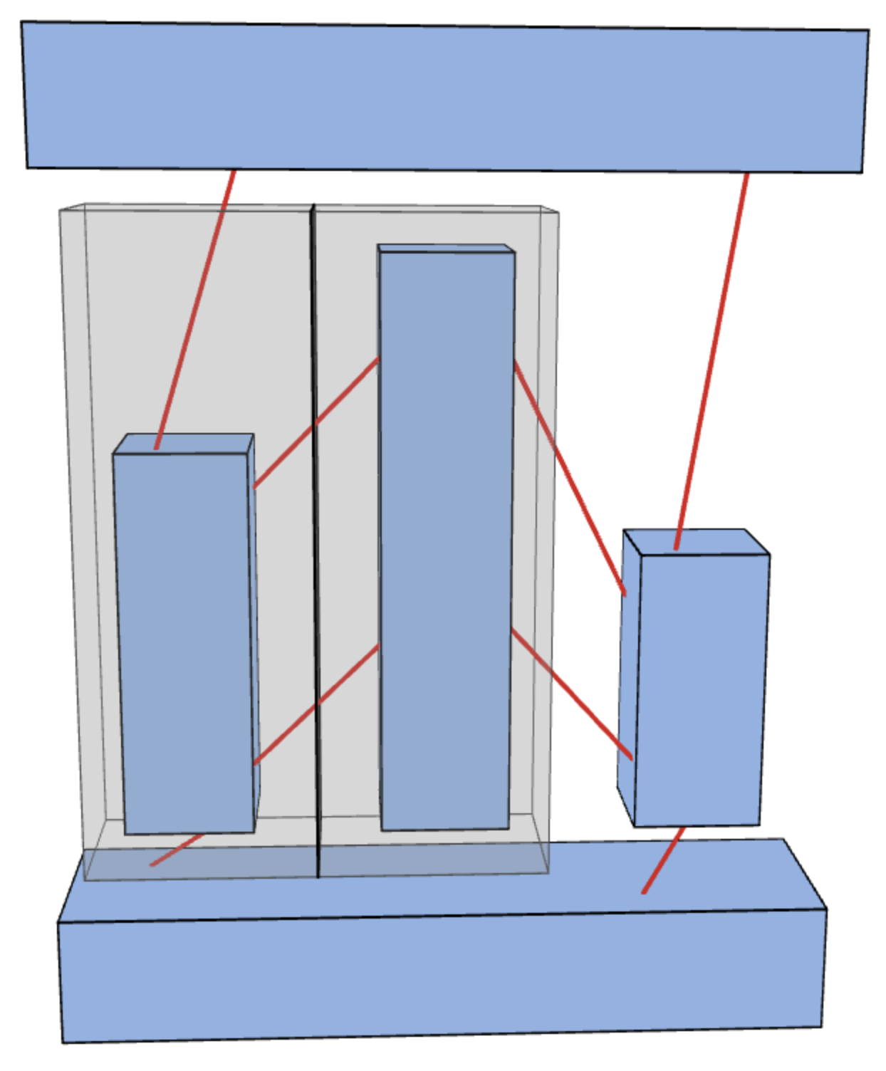
We progressively “merge” the different isolated regions. This can be seen in figure 17. Notice that figure 17(c) is the corresponding figure to figure 11.

Just as in lemma 1, a map can be created that glues all the interpolations on each merging process. Furthermore, the same analysis proves the weights depend only on the boundaries of these interpolations and does not change through them. Hence, in the above, we only need to verify what happens on them. An easy calculation shows that all of them have weight $4$ or $2$ . This can be visually confirmed bt seing the intersections of the edges with the boundaries in figure 17(c).

This doesn’t conclude our task. We must see that inside each isolated region the bounds are also preserved. For each one of the tangles, we can pick a point very close to the bottom face and make the homotopy to the surrounding prisms. One can assume, that except for the strands that go out of the prism, the tangle is entirely contained in the pyramid parallel to the upper face. This guarantees that the tangle is not cut into many different parts by different sides of the cube. This would bring the weight up. In this way, every level set cuts the tangle in three parts: the upper face cuts it when it enters, then it cuts it again when it goes out. However, it goes out through the paths going out of the surrounding prism. Hence, there are four cuts. We can see an example of this in figure 18.

In here, it is important to take good care of the thickening of the vertices. If we do not isolate them, then as we sweep we might intersect many at the same time. If several of them have artificial intersections they will make the count go up. This can be done, for example, with separating polyhedrons. A similar analysis works for the other two prisms (the horizontal ones) where the count is bonded by $2$ .

This concludes our sketch of proof. ∎

Remark 11.

That Pretzel knots have spherewidth bounded above by $4$ is probably well known. However, I searched online and with A.I. and it did not find explicit sources. It just repeatedly send me to [5, Figure 3].

Proposition 4 improves our bound $sw(3_{1})\leq 6$ . Indeed, $3_{1}=P(1,1,1)$ , and thus $sw(3_{1})\leq 4$ . This motivates the following:

Question 1.

Is there an embedding of the Pretzel knots in the finite iterations of the Sierpinski tetrahedron and a corresponding sphere decomposition that recovers the bound $4$ ?

This question seems dual to the upper bound of $6$ that we have found. Concretely, the finite connectivity between different tetrahedrons force the spherewidth to do not grow too much. However, it seems that at the same time, this same scarcity of options to change of tetrahedron forces the knot to visit pyramids for “superficial” purposes, creating intersections with the level set spheres that otherwise could have been avoided.

6.2 What other knots are there in the finite iterations?

In [3, Theorem II] it is proven that the only torus knots that are Pretzel knots are

	$\displaystyle T(2,n)$	$\displaystyle=P(1,...,1),$
	$\displaystyle T(3,4)$	$\displaystyle=P(3,3,-2)=8_{19},$
	$\displaystyle T(3,5)$	$\displaystyle=P(5,3,-2)=10_{124}.$

Notice all these torus knots indeed satisfy the conditions of theorem 2. There are many torus knots not in the above list, with $\min{p,q}\leq 9$ , and that are not Pretzel.

Ultimately, this leads to the following.

Question 2.

Can one describe in some sensible way what are the knots that appear in the finite iterations of the Sierpinski tetrahedron? This could entail a (hopefully?) finite list of families of knots with some understood exceptions.

Simpler versions of this question deal with finite concrete families. For example, is the family $T(3,n)$ for $n$ not a multiple of $3$ , in there? The first two members are because they are Pretzel knots.

Similarly, there are also knots that are neither Pretzel nor torus knots. The smallest prime example is $8_{21}$ . One of its knot diagram, taken from The Knot Atlas, is see in figure 19.

The diagram of figure 19 is very reminiscent of the combinatorial representations. At the moment of writing, I do not know if one can find it in some iteration.

In any case, more than torus knot families and Pretzel knots might be needed. What other family could be there lurking in the finite iterations?

Appendix A Geometric Lemmas on Polyhedrons

A.1 Interpolations

We will review several facts about interpolations of quadrilaterals in $\mathbb{R}^{3}$ . This results, or similar, are probably well known. However, we review them to highlight the aspects that we will require in our constructions.

Definition 11.

Given two points $A$ and $a$ in $\mathbb{R}^{3}$ , the interpolation between them is the continuous map $\alpha\mathrel{\mathop{\mathchar 58\relax}}[0,1]\longrightarrow\mathbb{R}^{3}$ given by

\alpha(t)=(1-t)A+ta.

The interpolation is a parametrization of the segment $Aa$ from $A$ to $a$ . The parameter $t$ represents the proportion $A\alpha(t)/Aa$ . Consequently, as long as $A$ and $a$ are different, this map is injective.

Given two segments $AB$ and $ab$ we can interpolate between them by “gluing” the interpolations at proportional corresponding sides. In other words, if $\alpha$ and $\beta$ interpolate $A$ to $a$ and, respectively, $B$ to $b$ , then

(1-s)\alpha(t)+s\beta(t),0\leq s\leq 1,

interpolates the segment from $\alpha(t)$ to $\beta(t)$ . This leads to

Definition 12.

Given two segments $AB$ and $ab$ the interpolation between them is the map

H(s,t)=(1-s)(1-t)A+(1-s)ta+s(1-t)B+stb,0\leq t,s\leq 1.

Remark 12.

To define the interpolation we must beforehand chose which endpoint of $AB$ goes to $a$ and which one to $b$ . We shall always tacitly assume they go in the corresponding order as they are written.

By construction, at fixed level $0\leq t_{0}\leq 1$ , the set given by

H(s,t_{0}),0\leq s\leq 1

is a line segment. At fixed level $s_{0}$ we get the parametrization

(1-t)((1-s)A+sB)+t((1-s)a+sb)

This is the interpolation $Aa$ to $Bb$ . However, the surface spanned by these interpolations itself is not necessarily contained in a plane. It is simply a doubly ruled surface (e.g. a saddle). We are speaking here in generic terms. Depending on the choice of points $A,a,B,b$ there can be self intersections and degenerations.

We are now ready to discuss the situation that we are interested in. We will have two flat quadrilaterals $ABCD$ and $abcd$ . In all the cases we will encounter later these polygons will be rectangles and, in a degenerate case, one shall be a point. However, let us keep the discussion somewhat general to handle all cases together.

Let $H(s,t)$ and $G(s,t)$ be the interpolations $AB$ to $DC$ and $ab$ to $dc$ . Then we can, once more, interpolate and get

F(s,t,u)=(1-u)H(s,t)+uG(s,t),0\leq u\leq 1.

Then $F$ is interpolating $ABCD$ towards $abcd$ .

Proposition 5.

Let $0\leq u_{0}\leq 1$ and define $A_{u_{0}},B_{u_{0}},C_{u_{0}}$ and $D_{u_{0}}$ be the points in the segments $Aa,Bb,Cc$ and $Dd$ dividing it in proportion $u_{0}$ . Then the map $(s,t)\mapsto F(s,t,u_{0})$ is the interpolation from $A_{u_{0}}B_{u_{0}}$ to $D_{u_{0}}C_{u_{0}}$ .

Proof.

By definition

	$\displaystyle H(s,t)$	$\displaystyle=(1-s)(1-t)A+(1-s)tD+s(1-t)B+stC,$
	$\displaystyle G(s,t)$	$\displaystyle=(1-s)(1-t)a+(1-s)td+s(1-t)b+stc.$

Substituting and rearranging we get $F(s,t,u_{0})$ equals

(1-s)(1-t)((1-u_{0})A+u_{0}a)+(1-s)t((1-u_{0})D+u_{0}d)+s(1-t)((1-u_{0})B+u_{0}b)+st((1-u_{0})C+u_{0}c).

The involved points

	$\displaystyle A_{u_{0}}\mathrel{\mathop{\mathchar 58\relax}}=$	$\displaystyle(1-u_{0})A+u_{0}a,$
	$\displaystyle D_{u_{0}}\mathrel{\mathop{\mathchar 58\relax}}=$	$\displaystyle(1-u_{0})D+u_{0}d,$
	$\displaystyle B_{u_{0}}\mathrel{\mathop{\mathchar 58\relax}}=$	$\displaystyle(1-u_{0})B+u_{0}b,$
	$\displaystyle C_{u_{0}}\mathrel{\mathop{\mathchar 58\relax}}=$	$\displaystyle(1-u_{0})C+u_{0}c,$

are those at which the segments $Aa,Dd,Bb$ and $Cc$ get divided into proportion $u_{0}$ . Furthermore, we recognize $F(s,t,u_{0})$ as the interpolation from, $A_{u_{0}}B_{u_{0}}$ to $C_{u_{0}}D_{u_{0}}$ . ∎

Definition 13.

In the context of the above discussion, let us call the interpolation $(t,s)\mapsto F(s,t,u_{0})$ the $u_{0}$ -th level interpolation and its image the $u_{0}$ -th level set of $F$ .

Proposition 6.

In the context of the above discussion, the following are hold:

1.

If $ABCD$ and $abcd$ are contained in parallel planes, then for all $0\leq u\leq 1$ the $u-th$ level sets is contained in a plane parallel to the planes of $ABCD$ and $abcd$ .
2.

If $ABCD$ and $abcd$ are parallelograms, maybe not parallel among themselves, then for all $0\leq u\leq 1$ the $u-th$ level sets is a parallelogram.

Proof.

We do them separately.

Proof of 1: There exists a vector $v$ perpendicular to $B-A,C-A,D-A$ and $b-a$ , $c-a$ and $d-a$ . This is because their corresponding planes are parallel.

We have seen before that

A_{u}=(1-u)A+ua,B_{u}=(1-u)B+ub

and thus

B_{u}-A_{u}=(1-u)(B-A)+u(b-a).

Hence, by linearity, $B_{u}-A_{u}$ is perpendicular to $v$ . In the same, fashion $C_{u}-A_{u}$ and $D_{u}-A_{u}$ are perpendicular to $v$ . Hence, we find that the four points are included in a plane through $A_{u}$ perpendicular to $v$ . The result follows as we have seen the interpolation $A_{u}B_{u}$ to $D_{u}C_{u}$ is a ruled surface and the sides are in this plane.

Proof of 2: We recall the reader that $XYWZ$ is a parallelogram if and only if

X+W=Y+Z.

By assumption then

A+C=B+D,a+c=b+d.

The result follows from the above equations by adding their appropriate linear combinations. Indeed,

A_{u}+C_{u}=(1-u)(A+C)+u(a+c)=(1-u)(B+D)+u(b+d)=B_{u}+D_{u}.

∎

Definition 14.

The image of $[0,1]^{3}$ under the map $F$ will be called the prismoid induced by $F$ . If no possibility of confusion can arise we will also call it the prismoid induced by the quadrilaterals $ABCD$ and $abcd$ .

Remark 13.

We are slightly abusing of notation. A prismoid usually refers to a particular type of solid of which the above examples sometimes might not belong.

Now, we must bring our attention to an important matter. When we have two segments $AB$ and $ab$ it is not true in general that the interpolation $H$ between them is injective or that the image of $H$ coincides with the interior of $ABba$ (if this is non intersecting).

Proposition 7.

Let $AB$ and $ab$ be two coplanar segments such that $ABba$ is a convex quadrilateral. Then the interpolation $H$ between them is injective.

Proof.

Suppose $H(s_{1},t_{1})=H(s_{2},t_{2})=p$ . Suppose that $s_{1}>s_{2}$ . We have said before that, at fixed level $s_{1}$ , $H(s_{1},\cdot)$ parametrizes a segment. This segments joins the corresponding points, at proportion $s_{1}$ , of opposite sides. By convexity, the whole segment is included in $ABba$ . In exactly the same way, there is a segment joining the corresponding points at proportion $s_{2}$ of the same opposite sides. The situation is thus as shown in the figure 20.

This configuration is impossible because on $Aa$ and $Bb$ , the interpolations are injective. Consequently, as the proportion grows the points should be closer to the endpoints. However, what we see is that in one $s_{1}$ is closer while in the other it is $s_{2}$ . This is a contradiction, thus $s_{1}=s_{2}$ .

A similar argument shows $t_{1}=t_{2}$ . ∎

Corollary 2.

Let $AB$ and $ab$ be two coplanar segments such that $ABba$ is a convex quadrilateral. Then the interpolation $H$ between them is an homeomorphism onto $ABba$ .

Proof.

The boundary of $[0,1]^{2}$ goes to the sides of $ABba$ . This is a simply connected curve and its interior is the quadrilateral (minus the edges). As $H$ is continuous, as it can be written as polynomials, we get its image is simply connected. Hence the map is surjective. We already know it is injective. We conclude $H$ is bijective. The closed map lemma implies $H$ is an homeomorphism onto its image. ∎

Proposition 8.

Let $ABCD$ and $abcd$ be two planar quadrilaterals. Let $F\mathrel{\mathop{\mathchar 58\relax}}[0,1]^{3}\longrightarrow\mathbb{R}^{3}$ be the interpolation thus constructed from $ABCD$ and $abcd$ . Let $\mathcal{S}=\text{Im}(F)$ . Suppose that $F$ is injective. Then there exists a surjective continuous map

\Phi\mathrel{\mathop{\mathchar 58\relax}}\mathcal{S}\longrightarrow[0,1],

such that for each $0\leq u\leq 1$ , the preimage $\Phi^{-1}(u)$ is the $u$ -th level set of $F$ .

Proof.

We emphasize that the content of this proposition is the existence and continuity of this map. For a point $p\in\mathcal{S}$ we define

\Phi(p)=u,

if $p=F(s,t,u)$ for some point $(s,t,u)$ . This is well-defined by the injectivity of $F$ . It is clearly surjective. By construction, the preimage of $u$ is the $u-$ th level map of $F$ as this is defined as

F(s,t,u),0\leq s,t,\leq 1.

Notice that we have the following diagram

The closed map lemma applied to $F$ implies that it is an homeomorphism onto its image (i.e. onto $\mathcal{S}$ ). Furthermore,

\Phi(F(s,t,u))=u,

by definition. Hence, $\Phi=(\Phi\circ F)\circ F^{-1}$ is continuous. ∎

Corollary 3.

Under the same conditions as those of proposition 8, the $u$ -th level sets of $F$ are topological disks.

Proof.

$F$ is an homeomorphism and the $u$ -th level set is the image of $[0,1]\times[0,1]\times\{u\}$ . ∎

Remark 14.

There are configurations of $ABCD$ and $abcd$ where the injectivity of $F$ fails spectacularly. In the cases we will work with, the situation is so concrete that the injectivity is easily verified from all the arguments we have discussed above.

A.2 A case where injectivity holds.

Now we describe a configurations we will find in our work and where injectivity holds.

Proposition 9.

Let $ABCD$ and $abcd$ be parallelograms in parallel planes and with their corresponding vertices named in consistent cyclic order. Suppose they satisfy the following conditions:

1.

$B-A$ and $b-a$ are positive scalar multiples of each other.
2.

$D-A$ and $d-a$ are positive scalar mulitples of each other.

Then the interpolation $F$ is injective.

Proof.

Let $0\leq u\leq 1$ be a fixed parameter. Define

	$\displaystyle A_{u}\mathrel{\mathop{\mathchar 58\relax}}=$	$\displaystyle(1-u)A+ua,$
	$\displaystyle B_{u}\mathrel{\mathop{\mathchar 58\relax}}=$	$\displaystyle(1-u)B+ub,$
	$\displaystyle C_{u}\mathrel{\mathop{\mathchar 58\relax}}=$	$\displaystyle(1-u)C+uc,$
	$\displaystyle D_{d}\mathrel{\mathop{\mathchar 58\relax}}=$	$\displaystyle(1-u)D+ud,$

the points which cut the segments $Aa,Bb,Cc$ and $Dd$ at proportion $u$ , respectively.

By assumption, we have the existence of two positive constants $\lambda,\mu>0$ such that

	$\displaystyle B-A$	$\displaystyle=\lambda(b-a)$
	$\displaystyle D-A$	$\displaystyle=\mu(d-a).$

A simple computation then shows

	$\displaystyle B_{u}-A_{u}$	$\displaystyle=(\lambda+u(1-\lambda))(b-a)=\left(1-u+\dfrac{u}{\lambda}\right)(B-A),$		(6)
	$\displaystyle D_{u}-A_{u}$	$\displaystyle=(\mu+u(1-\mu))(d-a)=\left(1-u+\dfrac{u}{\mu}\right)(D-A).$

Notice that

	$\displaystyle\lambda+u(1-\lambda)$	$\displaystyle=\lambda\left(1-u+\dfrac{u}{\lambda}\right)>0,$
	$\displaystyle\mu+u(1-\mu)$	$\displaystyle=\mu\left(1-u+\dfrac{u}{\mu}\right)>0.$

This implies that the triangle $A_{u}B_{u}D_{u}$ has positive volume, as its sides are positive multiples of those of $ABD$ . It also implies $A_{u},B_{u}$ and $D_{u}$ has the same orientation as $A,B$ and $D$ (and $a,b$ and $d$ ).

We have seen that, because the extreme faces are parallelograms, the intermediate $A_{u}B_{u}C_{u}D_{u}$ are also parallelograms. Nevertheless, we did not rule out they could be degenerate. However, the fact that $A_{u}B_{u}D_{u}$ has positive volume implies that it is nondegenerate because, being a parallelogram, its reflection $B_{u}D_{u}C_{u}$ must also have positive volume. We conclude that $A_{u}B_{u}C_{u}D_{u}$ is indeed a nondegenerate parallelogram. Hence, it is convex.

Now, suppose for a contradiction, that

F(s_{1},t_{1},u_{1})=F(s_{2},t_{2},u_{2}).

(7)

We have seen before that the $u$ -th level sets are planar and parallel to the quadrilaterals $ABCD$ and $abcd$ . Their corresponding vertices cut the segments $Aa,Bb,Cc$ and $Dd$ in proportion $u$ . Hence, if $u_{1}\neq u_{2}$ , these faces lie in different planes and the equality (7) cannot hold. On the other hand, if $u_{1}=u_{2}=u_{0}$ , then we have that

F(s_{1},t_{1},u_{0})=F(s_{2},t_{2},u_{0}).

However, proposition 7 implies that

(s,t)\mapsto F(s,t,u_{0}),

is injective. It is here where we needed convexity and nondegeneracy. Thus,

s_{1}=s_{2},t_{1}=t_{2}.

Hence, the map $F$ is injective. ∎

Remark 15.

The case where the opposite faces are parallel rectangles is covered in this proposition. The two conditions are to guarantee that the labels of the rectangles are consistent.

Furthermore, for rectangles we can say more. If $B-A$ and $D-A$ are orthogonal, then equations (6) imply that

(B_{u}-A_{u})\cdot(D_{u}-C_{u})=0.

Hence, all the level sets are also rectangles, as the only parallelograms with $90$ degree angles are rectangles.

A.3 Our main construction result

We are ready to prove our main result in this appendix. Let us first state the result.

Proposition 10.

Let $X\subset Y$ be in a $PP$ -configuration. Define

\mathcal{S}_{XY}\mathrel{\mathop{\mathchar 58\relax}}=\overline{Y-X},

1.

For each $0\leq u\leq 1$ , $\Phi^{-1}(u)$ is a rectangular prisms with faces parallel to those of $Y$ . In particular, it is a polyhedral sphere $\mathbb{S}^{2}$ .
2.

$\Phi^{-1}(0)=X$ and $\Phi^{-1}(1)=Y$ .

This results holds if $X$ is a point. The only change is the inequality in property $1$ should be $0<u\leq 1$ .

We will do the nondegenarte case, that is, when $X$ is not a point. We leave the adaptation of the results to the degenerate case to the reader.

We will have some preparation before we show the proof. Let us suppose we have two rectangular prisms $P_{1}$ and $P_{2}$ in a $PP$ -configuration. We can divide $\mathcal{S}_{P_{1},P_{2}}$ in different regions, each of which is covered by one of our previous constructions. We see this division in figure 21. We realize there are six prismoids in which we divide $\mathcal{S}_{P_{1},P_{2}}$ .

For each of these prismoids $\mathcal{R}$ , propositions 9 implies that the corresponding $F$ is injective. Consequently, proposition 8 implies the existence of a continuous surjective map

\Phi_{\mathcal{R}}\mathrel{\mathop{\mathchar 58\relax}}\mathcal{R}\longrightarrow[0,1]

with $\Phi^{-1}(u)$ equal to its $u$ -th level set. Our goal is to use the gluing lemma to build out of them a map

\Phi_{P_{1},P_{2}}\mathrel{\mathop{\mathchar 58\relax}}\mathcal{S}_{P_{1},P_{2}}\longrightarrow[0,1].

We will then verify that this map satisfies the requirements we want.

Our first order of business is to prove the hypothesis of the gluing lemma. That is, we must understand the intersections of the prismoids and prove that on them their corresponding maps coincide.

Proposition 11.

Suppose $ABCD,abcd,BCEH$ and $bceh$ are four planar convex quadrilaterals satisfying the following assumptions:

1.

$BCcb$ is a planar convex quadrilateral contained in the plane $L$ .
2.

The points $A,D,a,d$ lie on different open half space of $L$ than the points $E,H,e,h$ .

Let $F$ be the interpolation from $ABCD$ to $abcd$ and $G$ the one from $BCEH$ to $bceh$ . Then, the prismoids associated to $F$ and $G$ intersect exactly in their common face $BCcb$ .

Proof.

Suppose that $F(s_{1},t_{1},u_{1})=G(s_{2},t_{2},u_{2})$ . We have seen that the maps

	$\displaystyle u$	$\displaystyle\longmapsto F(s_{1},t_{1},u),\;0\leq u\leq 1,$
	$\displaystyle u$	$\displaystyle\longmapsto G(s_{2},t_{2},u),\;0\leq u\leq 1,$

are parametrization of segments. In other words, they are the interpolation from $F(s_{1},t_{1},0)$ to $F(s_{1},t_{1},1)$ and, respectively, $G(s_{2},t_{2},0)$ to $G(s_{2},t_{2},1)$ .

The first interpolation $F(s_{1},t_{1},u)$ has its endpoints on the quadrilaterals $ABCD$ and $abcd$ . Because $ABCD$ and $abcd$ are convex quadrilaterals, and halfplane are convex themselves, these points are on the closed halplane that contains $ABCD$ and $abcd$ . Consequently, the whole interpolation lies in this closed half plane. Analogously, the whole interpolation $G(s_{2},t_{2},u)$ lies on the other closed halfplane.

The given situation is only possible if both segments lie on $L$ themselves. In particular, the intersection point lies on $L$ . Furthermore, because $A,D,a,d$ are on the open half space (i.e. not on $L$ ), the only points of their corresponding prismoid on $L$ are the points of $BCcb$ . Analogously for the other prismoid. We conclude, the intersection point lands on the face $BCcb$ .

On the other hand, because both prismoids share the vertices $B,C,c,b$ , and this quadrilateral is convex, we know by construction the interpolation $BC$ to $bc$ spans the whole quadrilateral.

Thus, by double inclusion, the intersection of these prismoids is exactly their common face. ∎

Remark 16.

Notice that the injectivity of the prismoids is not necessary for this proof.

All the cases we have to consider are covered by proposition 11. The opposite faces are two rectangles with parallel faces. The face their share is formed from an interpolation between two segments that are parallel.

Proposition 12.

The set of six maps $\Phi_{\mathcal{R}}\mathrel{\mathop{\mathchar 58\relax}}\mathcal{R}\longrightarrow[0,1]$ glue to a map $\Phi\mathrel{\mathop{\mathchar 58\relax}}\mathcal{S}_{P_{1},P_{2}}\longrightarrow[0,1]$ .

Proof.

By propositions 11, we know that the six prismoids that comprise $\mathcal{S}_{P_{1},P_{2}}$ intersect at their corresponding face. Each of this intersections is itself an interpolation from one segment to another. In particular, the definition of the map in these faces depends on the segments interpolated and not on the quadrilaterals to which they belong.

We have already explained why each of the maps $\Phi_{\mathcal{R}}$ exists. Ultimately, it is because in the situations we are, we know the interpolation $F_{\mathcal{R}}$ is injective. Consequently, by construction, if a point $p$ in such prismoid is in the $u$ -th level face, we have

\Phi_{\mathcal{R}}(p)=u.

Suppose two of these prismoids $\mathcal{R}_{1}$ and $\mathcal{R}_{2}$ intersect at the face $XYyx$ , where $XY$ is one edge and $xy$ is the corresponding opposite edge. Then the intersection of the $u$ -th level face, of either prismoid, with the shared face is the segment $X_{u}Y_{u}$ , where $X_{u}$ and $Y_{u}$ have their usual meaning (i.e. the points that divide $Xx$ and $Yy$ in proportion $u$ ). We know that every point on the shared face lies in a unique segment $X_{u}Y_{u}$ and that the value of $u$ depends only $XYyx$ , and not on the prismoid. We conclude,

\Phi_{\mathcal{R}_{1}}(X_{u}Y_{u})=u=\Phi_{\mathcal{R}_{2}}(X_{u}Y_{u}).

That is, $\mathcal{R}_{1}$ and $\mathcal{R}_{2}$ coincide on the shared face. This concludes our proof. ∎

We are finally ready to prove othe main result of this appendix.

Proof of proposition 10.

By proposition 12 we have the existence of a continuous map

\Phi\mathrel{\mathop{\mathchar 58\relax}}\mathcal{S}_{P_{1},P_{2}}\longrightarrow[0,1].

In each one of the prismoids $\mathcal{R}$ it coincides with $\Phi_{\mathcal{R}}$ . To conclude, we must prove the properties hold. We do them separately.

Property 1: For each $0\leq u\leq 1$ , $\Phi^{-1}(u)$ is a rectangular prism with faces parallel to those of $Y$ . In particular, it is a polyhedral sphere $\mathbb{S}^{2}$ .

For each $0\leq u\leq 1$ , the level set $\Phi^{-1}(u)$ consists of the union of the six level set faces $\Phi_{\mathcal{R}}^{-1}(u)$ as $\mathcal{R}$ varies on the ten prismoids. We know that for each case the level sets are rectangles, each of which glues on each of its edges to another one on the common face of the prismoids that contain them. We know by propositions 11, that the pairwise intersections, at the fixed level $t$ , consists only on these edges. Consequently, we have a polyhedron with six faces, each of which is a rectangle.

The only thing that we have to do is to compute its Euler Characteristic. There are six faces. The number of vertices is $8$ , as there is one per edge joining corresponding vertices on $P_{1}$ and $P_{2}$ . Finally, the number of edges are $12$ . Indeed, there are four per face but each is counted twice. We have

\text{Vertices}-\text{Edges}+\text{Faces}=8-12+6=2.

We conclude this is a sphere.

(What we are verifying is that there is no boundary. Since each face is moving at different pace, because the prisms are not homothetic, one might imagine there is a weird case where some faces fail to close.)

Property 2: $\Phi^{-1}(0)=P_{1}$ and $\Phi^{-1}(1)=P_{2}$ .

This follows from the fact that this holds for each interpolation. The beginning face, which is the $0$ -th level face is a face of the $P_{1}$ . The $1$ -th level face is on $P_{2}$ . ∎

References

[1] J. Broden, M. Espinosa, N. Nazareth, and N. Voth (2026) Knots inside fractals. Experimental Mathematics 0 (0), pp. 1–19. External Links: Document Cited by: §1.1, §1.1, §1.3, §1.3, §1.4, §5.2, §6.1.
[2] G. Hinojosa, U. Morales-Fuentes, R. Valdez, and A. Verjovsky (2026) Wild knots embedded in the menger sponge. External Links: 2602.20384 Cited by: §1.3, §1.4.
[3] A. Kawauchi (1985) Classfication of pretzel knots. Kobe journal of mathematics 2, pp. 11–22. External Links: Link Cited by: §6.2.
[4] F. Kobayashi (2021) Uniform convergence and knot equivalence. External Links: 2101.04106 Cited by: §1.3.
[5] C. Lunel and A. de Mesmay (2026) A structural approach to tree decompositions of knots and spatial graphs. Algebraic & Geometric Topology 26 (6), pp. 2015–2047. External Links: ISSN 1472-2747, Document Cited by: §1.1, §1.1, §1.2, §1.3, §1.4, §3.2, §3.3, §3, §4.6, Remark 11.
[6] S. Schleimer, A. de Mesmay, J. Purcell, and E. Sedgwick (2019) On the tree-width of knot diagrams. Journal of Computational Geometry 10 (1), pp. 164–180. External Links: Document Cited by: §1.3, §1.4.
[7] M. A. Shtan’ko (1971) Solution of menger’s problem in the class of compacta. Doklady Akademii Nauk SSSR 201 (6), pp. 1299–1302 (Russian). Note: English translation: Soviet Mathematics. Doklady, 12 (1971), 1846–1849 External Links: MathReview Entry Cited by: §1.3, §1.4.

Knots and the Sierpinski tetrahedron

Abstract

1 Introduction

1.1 Motivation and main results

Theorem A.

Definition A.

Definition B.

Definition C.

Theorem B.

1.2 Organization of this paper

1.3 Discussion on some previous literature and some comments

1.4 A.I. use disclosure

1.5 Ackwonledgements

2 Some geometric observations on polyhedra

2.1 A discussion on polyhedrons

Definition 1.

Proposition 1.

Proof.

Remark 1.

Remark 2.

3 Sphere decomposition and spherewidth

3.1 Review of the main concepts: double bubbles

Definition 2.

3.2 Review of the main concepts: thickening and transversality

Definition 3.

Remark 3.

Definition 4.

Definition 5.

3.3 Review of the main concepts: sphere decompositions

Definition 6.

Remark 4.

Definition 7.

Definition 8.

Remark 5.

Remark 6.

4 Sphere Decomposition induced by the Sierpinski tetrahedron

4.1 The change of 11-skeleton

Definition 9.

Definition 10.

4.2 The thickening of the vertices

Remark 7.

4.3 The subdivision

Example 1.

Proposition 2.

Proof.

4.4 The tree for an intermediate region

Lemma 1.

Proof.

Proposition 3.

Proof.

Corollary 1.

Proof.

4.5 The vertex cubes

Lemma 2.

Proof.

Remark 8.

4.6 The main theorem

Theorem 1.

Proof.

Remark 9.

Theorem 2.

Proof.

5 An example with the Trefoil

5.1 Intermediate regions and the combinatorial representation

5.2 The example for the trefoil

Remark 10.

6 Further Questions and Concluding Remarks

6.1 Pretzel Knots

Proposition 4.

Proof.

Remark 11.

Question 1.

6.2 What other knots are there in the finite iterations?

Question 2.

Appendix A Geometric Lemmas on Polyhedrons

A.1 Interpolations

Definition 11.

Definition 12.

Remark 12.

Proposition 5.

4.1 The change of $1$ -skeleton