Phase diagram morphology shapes droplet propulsion in chemical gradients
Abstract
Droplets in complex environments often encounter compositional gradients that drive their propulsion. For example, surfactant gradients induce surface-tension-driven propulsion via the Marangoni effect. Here, we show that such propulsion emerges generically, even in the absence of surfactants. Employing a thin-interface approximation, we derive a compact expression for the droplet velocity in terms of droplet size, viscosity, the sensitivity of surface tension to a regulating component, and the chemical potential gradient of that component. Our theory reveals that droplets move toward regions of lower stability, as encoded in the morphology of the phase diagram, particularly near critical points. Numerical simulations confirm these results, which establish a general route to predicting and designing droplet motility from the phase behavior of complex fluids.
I Introduction
Phase-separated droplets are subject to complex environments in biological [1, 2, 3, 4, 5] and synthetic systems [6, 7, 8, 9, 10], where they are exposed to gradients of temperature, material properties, and various chemical species. Droplets respond to these gradients, either through diffusive mechanisms that translate droplets without momentum transport [11, 2, 12], or through advective mass flows. Such mass transport can be driven externally, e.g., via gravity or other body forces, or internally, e.g., by motile active matter [13] and other forms of activity [14]. One interesting case involves surface tension gradients [15, 9, 16], which transform energy stored in chemical gradients into droplet propulsion. Understanding this type of propulsion is important for applications in microfluidics, such as lab-on-a-chip devices [17, 18], and for elucidating momentum transport in biomolecular condensates [1].
Droplet propulsion driven by surface tension, also known as Marangoni propulsion, has been studied extensively in the context of surfactants [9, 19, 6, 20, 8, 21, 22], where surface tension gradients arise from heterogeneous distributions of surfactants that adsorb onto the droplet interface. Propulsion is also possible without surfactants, e.g., in temperature gradients [23, 24] or gradients of regulating species [25, 26, 27]. Such phenomena have been modeled by assuming that the regulating field either directly controls surface tension [23, 28, 20, 16, 22], or only affects the capillary stress [24, 27, 19]. In these cases, the concentration fields of the regulator and droplet components are not treated on equal footing, and surface tension is prescribed, rather than emerging from interactions between components. However, recent experiments [25, 26, 27] have shown that the phase behavior, encoded by interactions between components, strongly informs the motion of droplets in compositional gradients, a feature not captured by current theories.
To understand how interactions between molecular components give rise to gradients in surface tension, and thus droplet propulsion, we develop a framework that connects thermodynamic phase behavior to the interfacial stresses driving advective flows. We find that a semi-grand-canonical picture is advantageous for obtaining accurate predictions of droplet velocity. This approach reveals that droplets tend to move toward regions where they would dissolve, a phenomenon known as dialytaxis [25]. We show that the equilibrium phase diagram shapes the direction of droplet motion.
II Results
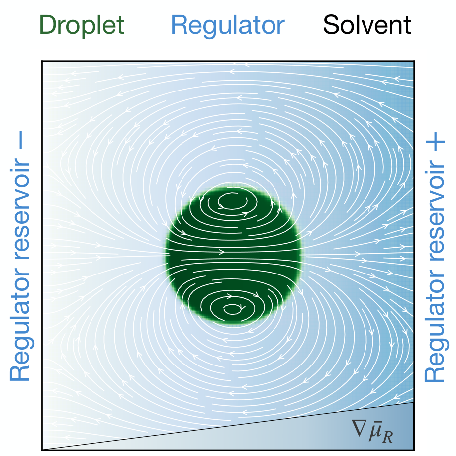
To study the motion of droplets in compositional gradients, we first introduce numerical simulations of a diffuse-interface model, which we then compare to analytical predictions from a thin-interface model to predict the propulsion velocity.
II.1 Externally imposed gradients propel droplets
II.1.1 Thermodynamics
Before considering external gradients, we first introduce key concepts in a simple equilibrium system. We consider an isothermal, incompressible system comprising different components and a solvent species. The system’s state is described by the volume fractions of all components, whereas the solvent fraction follows from the no-void condition, . The equilibrium state minimizes the free energy , where
| (1) |
is the free energy density. Here, is the thermal energy, is a reference molecular volume, denotes the local part of the energy density, and the constant, symmetric matrix penalizes gradients.
Minimizing can lead to multiple coexisting phases [5, 29]. In thermodynamically large systems, these phases must exhibit chemical equilibrium, which demands equal exchange chemical potentials , where are the molecular volumes of the components. Moreover, the phases must obey mechanical equilibrium, which implies equal osmotic pressures . In finite systems, we additionally need to account for interfaces, across which the pressure can vary. Mechanical equilibrium then implies , with the associated stress [5]
| (2) |
where the first term accounts for osmotic pressure , whereas the second term captures interfacial contributions. In particular, interfaces between phases exhibit a surface tension , which follows from the excess stress [30]
| (3) |
where the integral is along the normal direction across the interface, while denotes a tangential direction. Since creating an interface costs an energy per unit area [31], equilibrium systems minimize interfacial area, implying spherical droplets. The pressure inside such a droplet is increased by the Laplace pressure [5], where is the sum of principal curvatures of a spherical droplet of radius in dimensions. Consequently, mechanical equilibrium becomes .
II.1.2 Kinetics
The system is driven out of equilibrium when we apply a gradient by coupling the system to different particle reservoirs at the boundaries at and (Fig. 1). We achieve this by imposing exchange chemical potentials, , describing the exchange of some species with solvent across the boundary. The chemical potential difference then drives a flux of species through the system. In contrast, we impose no-flux conditions for all other species, so that their total volume is conserved.
To understand the behavior of this non-equilibrium system, we next investigate the dynamics of all volume fractions . Since all components are locally conserved, can only change by center-of-mass advection or by relative fluxes driven by gradients in chemical potentials,
| (4) |
where are the diffusive mobilities. The center-of-mass velocity field satisfies momentum conservation
| (5) |
where the term in brackets is the total stress comprising viscous stress, given by the product of viscosity and the rate-of-strain tensor , isotropic hydrostatic pressure to enforce incompressibility , and given by Eq. (2). In contrast to the equilibrium situation we discussed above, is generally non-zero in a system driven out of equilibrium. Taken together, Eqs. (1)–(5) can describe droplets in externally imposed gradients.
II.1.3 Numerical simulations
To build intuition for the behavior of our system, we consider components and a solvent with equal molecular volumes, where reservoirs impose a gradient of a regulator component , which affects a segregating droplet component . We describe the interactions between the components by a Flory–Huggins free energy density, , for with solvent fraction . We choose the interaction parameters such that segregates from , whereas does not create its own phase. To define the free energy density given by Eq. (1), we also require the gradient penalty matrix to be positive definite to enable stable interfaces. For simplicity, we choose proportionally to the reduced interaction matrix after eliminating the solvent via the no-void condition, for , where is the interfacial width. This choice captures that and both originate from the same microscopic interactions; the concrete form can be derived from a lattice model [32, 33]. Finally, we choose density-dependent mobilities , which capture the correct cross-diffusivities in incompressible systems [5, 34, 35]. Here, the bare mobility controls the overall diffusive mobilities and allows us to define a fundamental time scale , which governs the dynamics of passive droplets.
To impose a regulator gradient, we consider a two-dimensional, rectangular setup with periodic boundary conditions in the -direction, and reservoir boundary conditions for at the left and right wall, at and (Fig. 1). Moreover, we impose vanishing normal derivatives, , which implies that all components (including solvent) interact equally with the walls at the reservoirs [5]. We solve Eq. (4) using a finite difference scheme, whereas the velocity field is determined using a projection method; see Appendix section A. As expected, we find that the regulator exhibits a gradient between the reservoirs, whereas the droplet component is strongly enriched in a near-spherical droplet (Fig. 1). The associated velocity field exhibits two vortices, which propel the droplet toward the right, i.e., toward larger regulator concentrations. It has been proposed that this tendency is caused by the fact that the regulator tends to dissolve the droplet [25]. Using a detailed analysis of droplets in gradients, we will show that this is indeed generally the case.
II.2 Surface tension gradients set droplet velocity

To understand the propulsion of the droplet, we analyze the velocity field , which is driven by gradients in the stress tensor given by Eq. (2). Since contributions from the osmotic pressure can be absorbed by the hydrostatic pressure , we write , to emphasize that the velocity field is determined by the gradient contribution . Since compositional gradients in the bulk are small compared to interfacial gradients, is localized to the droplet interface (Fig. 2A). Consequently, is driven by interfacial effects, and we hypothesize that surface tension gradients drive the flow via the Marangoni effect.
To show that is driven by surface tension gradients, we introduce a thin-interface approximation, exploiting the localized stress at the interface. Far away from the interface, the velocity field obeys
| (6) |
where absorbs the osmotic pressure and enforces incompressibility . To obtain a velocity field everywhere, Eq. (6) is solved separately inside and outside the droplet with appropriate boundary conditions. For simplicity, we assume that the pressure is uniform far away, implying that flows are exclusively driven by the stress at the interface and not by externally applied pressure gradients. At the droplet interface, we assume continuous velocity fields () and that the interface is in local equilibrium. This allows us to identify jump conditions for the viscous stress (Appendix section B and reference [36]),
| (7a) | ||||
| (7b) | ||||
while follows from incompressibility. The first condition states that the jump of the normal component of the viscous stress across the interface is given by the Laplace pressure , which is proportional to the sum of principal curvatures of the interface, . In contrast, tangential stresses follow from the surface gradient of the surface tension . Note that the boundary conditions given by Eq. (7) can also be interpreted as a force density field localized at the interface, so that is governed by in the entire system. Taken together, in the thin-interface approximation, the velocity field is entirely controlled by the surface tension along the interface.
To determine the droplet velocity , we define the droplet as an isocontour of the associated volume fraction field . The velocity is then given as the time derivative of the center-of-mass of the contour. Assuming that the contour is predominantly moved by advection, we find , where the integral is over the surface of the droplet of volume [37]. In the case of a near-spherical droplet in a system of constant viscosity , this simplifies to [16, 38]
| (8) |
where is the radial unit vector in spherical coordinates centered at and the integral is taken over the whole solid angle . Here, and capture pre-factors based on dimension . If the viscosity inside the droplet differs from the viscosity outside, the entire prefactor in front of the integral differs, e.g., for [16]. Note that vanishes for a solid sphere (), where instead diffusiophoresis becomes relevant [39, 40]. In contrast, for a fluid-like droplet, Eq. (8) shows that variations in surface tension set the droplet velocity.
II.3 Local chemical potential sets surface tension
To use Eq. (8) to determine the droplet velocity , we must determine how surface tension varies along the droplet interface. Numerical simulations indicate that depends roughly linearly with the distance along the gradient (Fig. 2B). Since is determined via Eq. (3), the variation of must originate from variations of the thermodynamic variables. In principle, we could thus express as a function of volume fractions , the chemical potentials , or a combination since all fields vary in space (Fig. 2C,D). To identify a natural description, we consider global conservation: The overall amount of droplet material is conserved, suggesting a canonical ensemble with as the natural variable. In contrast, the regulator is controlled by external reservoirs, corresponding to a grand-canonical ensemble and natural variable . We thus hypothesize that controls the coexisting fractions of droplet material, and thus the associated surface tension , at each point in space.

To see whether we can determine surface tensions by focusing on the chemical potential of the regulator, we next determine the associated phase diagram. Fig. 3A shows tie lines (thin gray lines) connecting coexisting compositions of droplet material (green line) as a function of . In this semi-grand-canonical case, tie lines must be vertical to have identical in both phases. This also implies that selects a unique pair of coexisting compositions, which would not have been the case in a canonical phase diagram where we vary . In our example, raising lowers the compositional difference until phase separation ceases completely at the critical point. This influence of is directly visible in our spatially resolved simulations (Fig. 2C). Since uniquely determines coexisting phases, it also governs the full interface profiles if is given. We can thus use simple thermodynamic equilibrium calculations (see Appendix section F), and Eq. (3) to determine the surface tension as a function of (Fig. 3B). Note that such an association would be impossible if we focused on the regulator fraction in a canonical ensemble since changes strongly across the interface. Taken together, the semi-grand-canonical approach allows us to associate coexisting fractions and surface tension with each value of and thus each position .
Using the dependence of surface tension on the regulator potential , we can further simplify the expression for the droplet velocity . In particular, assuming that the regulator gradient is quasi-stationary and that variations in and are small, we have , with for . Using Eq. (8), we thus find for two dimensions
| (9) |
where all quantities are evaluated at the droplet position . In three dimensions, the prefactor becomes . Eq. (9) clearly shows that larger droplets move faster, whereas higher viscosities slow them down. Additionally, the velocity is determined by the variation of surface tension and the chemical potential gradient.
To test whether the prediction given by Eq. (9) is reasonable, we compare it to our numerical simulations. We use the same setup as before (section II.1.3) and run simulations of droplets with various radii for different externally imposed gradients. We determine droplet positions and radii by fitting a spherical shape and determine the instantaneous velocity for various time points . We then average the normalized velocity for a short time period (after an initial transient) to estimate the normalized droplet velocity (see Appendix Fig. S3). To obtain a non-dimensional quantity, we report in units of the time it takes for a particle to diffuse across the interface (Fig. 3E). Consequently, the observed low magnitudes are consistent with our assumption of quasi-stationarity. The measured speed increases with the chemical potential difference of the regulator between the two reservoirs, consistent with the last factor in Eq. (9). Similarly, the fact that data for different radii collapses confirms the expected linear scaling with . These observations confirm that Eq. (9) captures important qualitative aspects of droplet motion.
To quantitatively compare our numerical data to the prediction by Eq. (9), we estimate and . The first term follows directly by differentiating , which we obtained from the equilibrium considerations above (Fig. 3B,C). In contrast, the potential gradient depends on the concrete compositions in the system. Fig. 2D suggests that is a linear function of the position along the gradient both inside and outside the droplet, which is consistent with a stationary solution of the diffusion equation with weakly varying mobilities, . To estimate the required gradient inside the droplet, we consider a one-dimensional approximation, where is a piecewise linear function. This function is uniquely defined given the overall chemical potential difference , system size , droplet radius , and the respective mobilities , which we determine from (see Appendix section E). Since depends on densities, this procedure captures the physical effect that the potential gradient, and thus the droplet velocity, depend on the enrichment of the regulator in the droplet, which is controlled by the interaction matrix . Taken together, these ideas allow us to use Eq. (9) to predict without running a detailed simulation of Eqs. (4)–(5). This prediction slightly overestimates the numerically measured values (Fig. 3E), although it captures all trends in the numerical data, suggesting that the approximations that led to Eq. (9) capture the essence of the physical processes. Interestingly, the analytical theory identifies a clear maximum in the velocity at intermediate chemical potentials .
The maximal velocity at intermediate values of originates from a non-monotonic dependence of on (Fig. 3C). Such non-monotonic behavior is universal since must vanish for very small and very large values of : On the one hand, the influence of the regulator must vanish in the binary limit (, ). On the other hand, the system is close to the critical point for large , where the surface tension exhibits the mean-field scaling [41]. Note that the scaling exponent is the same as for temperature [32, 42], since the chemical potential difference scales proportional to the temperature difference to leading order as a consequence of field mixing [43, 44]. This scaling implies that vanishes for . Since exhibits finite values while vanishing at extreme values of , its absolute value must assume a maximum, which implies a maximal speed given by Eq. (9). These properties do not depend on particular parameters, suggesting that knowledge of critical points is crucial to predict droplet propulsion.
II.4 Morphology of phase diagrams determines the motion of droplets
To see whether the location of critical points is a robust predictor of droplet motion, we consider various phase diagrams with qualitatively different morphologies. So far, we have considered a phase diagram in which increasing the regulator potential destabilizes droplet formation (Fig. 3A). Since the regulator was dilute, this implied that the droplet moved toward regions of denser regulator (higher ). In contrast, we could also consider systems in which the regulator stabilizes droplets, which implies a qualitatively different phase diagram (Fig. 4A). The associated surface tension now increases with (lower panel), such that Eq. (9) predicts that the droplet moves toward lower . In both cases, the droplet thus moves toward the critical point, where surface tension vanishes.
Next, we consider more complex phase diagrams. Fig. 4B shows a case of segregative phase separation between droplet material and regulator, which exhibits two critical points. Since this case involves strong attraction (), the corresponding would not be positive definite, and we thus choose independent of in this case. In any case, the surface tension vanishes at the two critical points, implying the associated depends non-monotonically on (lower panel). The direction of droplet propulsion depends on : For low , the droplet moves toward the left critical point, whereas for large , it moves toward the right one. Consequently, in the same gradient, droplets can move in opposite directions depending on the location along the gradient.
We also note the existence of phase diagrams without critical points: Fig. 4C shows a generic example where the droplet material segregates from solvent and regulator. Here, also exhibits a non-monotonic dependence on , although with the opposite curvature compared to panel B. Consequently, droplets move toward the center of the phase diagram, where is minimal. Between these two cases is a marginal case (Fig. 4D), where solvent and regulator have identical physical properties ( and ). This case is essentially binary phase separation between droplet material and the other species, implying that the phase diagram and do not depend on the relative fractions of solvent to regulator, and externally imposed regulator gradients do not induce propulsion. Note that this result relies on the connection between and described in section II.1.3. This relation is not necessarily accurate for complex molecules, which could lead to surface tension gradients even when the phase diagram predicts none (see Appendix section G). However, since surface tensions must vanish at critical points, these details have little influence on the qualitative conclusion that the morphology of the phase diagram shapes the propulsion of the droplet.
In the simplest case, the morphology of phase diagrams is controlled by critical points (Fig. 4A,B), and the droplet generally moves toward those. However, even if the phase diagram does not possess critical points (Fig. 4C), we can use qualitative information on how phase diagrams depend on interaction parameters to deduce the direction of droplet propulsion: The particular phase diagram shown in Fig. 4C is closely related to a case with two 2-phase regions, where droplet material segregates either from solvent or regulator, while these two species repel each other (large , Fig. 5A). The corresponding critical points are close to the center of the phase diagram, implying that droplets would move toward the center in either 2-phase region. Decreasing morphs the phase diagram toward the one shown Fig. 4C, demonstrating that they are closely related. In particular, the phase diagram inherits the direction of droplet propulsion, even though the critical points disappeared. This behavior persists until vanishes at the marginal case (Fig. 4D). Taken together, the presence of critical points at nearby parameter values informs the phase diagram morphology and thus droplet propulsion in chemical gradients. As a rule-of-thumb, droplets perform dialytaxis [25], i.e., they move toward their dissolution.
III Discussion
In this work, we have described surface-tension-driven propulsion of a droplet in a regulator gradient. In contrast to previous literature [23, 15, 24, 16, 45, 38], surface tension is not prescribed, but emerges from the interactions of droplet components, solvent, and regulator, which are all treated as continuous fields. We found that this situation is best described in a semi-grand-canonical ensemble, where the surface tension is evaluated as a function of the chemical potential of the regulator. A regulator gradient then implies a surface tension gradient, which propels the droplet via the Marangoni effect. We derived a compact expression for the droplet velocity in Eq. (9), showing that, qualitatively, is determined by the equilibrium phase diagram via (Fig. 4). Quantitatively, can be affected by multiple parameters: First, by the viscosity of the mixture. Second, by droplet size , which is determined by the total amount of droplet material. Third, by , whose magnitude is governed by the average surface tension and whose form is determined by the interaction matrix , and thus tightly linked with the phase diagram. Fourth, by the non-equilibrium drive in the form of , which is controlled by the externally applied gradient and modified by the partition coefficient of the regulator.
To estimate the propulsion speed quantitatively, we consider two example experimental systems. The first system comprises P granules that segregate in MEX-5 gradients in C. elegans embryos [1]. These granules have typical radii of and exhibit relatively large ratios of viscosity to surface tension, , possibly because the complex interface implies small [46]. To estimate the maximal velocity, we assume that surface tension vanishes on one side of the cell of length , implying . This velocity is small (e.g., compared to flows in the embryo on the order of [1]), so surface-tension-driven propulsion is negligible in P granule segregation. The second system concerns the strong self-propulsion of BSA droplets in pH gradients [25]. Here, typical parameters are , , , , and , leading to , consistent with measurements [25]. These examples show that the in vitro BSA system exhibits velocities that are roughly three orders of magnitude larger than those in the in vivo P granule system. While the in vitro system exhibits much smaller ratios , gradients are also applied over larger distances, so that these two effects roughly compensate. The velocity difference is thus mainly due to the size disparity of droplets.
So far, we have only considered the simplest case of an isolated droplet in a single regulator gradient in the limit where diffusion-based drift is negligible [11, 2, 12]. Since drift can lead to self-propulsion [47] and interactions between droplets [48], we expect similar effects from hydrodynamic propulsion, potentially including nonreciprocal interactions [49]. Furthermore, our theory can be readily generalized to multiple chemical potential gradients in -component systems with a single droplet forming component. Moreover, propulsion in realistic droplets might be affected by viscoelasticity [50, 51, 52, 53, 54] and surfactants [9, 19, 6, 20, 8, 21, 22]. Finally, self-generated gradients, e.g., from evaporation [10, 55] or chemical reactions [25, 27, 14], could lead to additional dynamical phenomena.
Acknowledgements.
We thank Gregor Häfner, Marcus Müller, Oliver Paulin, Kaarthik Varma, and Eric R. Dufresne for fruitful discussions. We gratefully acknowledge funding from the Max Planck Society. S. K. acknowledges funding from a fellowship of the IMPRS-PBCS. S. K. acknowledges support by the study program “Biological Physics” of the Elitenetzwerk Bayern.References
- [1] C. P. Brangwynne, C. R. Eckmann, D. S. Courson, A. Rybarska, C. Hoege, J. Gharakhani, F. Jülicher, and A. A. Hyman, Germline P Granules Are Liquid Droplets That Localize by Controlled Dissolution/Condensation, Science 324, 1729 (2009).
- [2] S. Saha, C. A. Weber, M. Nousch, O. Adame-Arana, C. Hoege, M. Y. Hein, E. Osborne-Nishimura, J. Mahamid, M. Jahnel, L. Jawerth, A. Pozniakovski, C. R. Eckmann, F. Jülicher, and A. A. Hyman, Polar Positioning of Phase-Separated Liquid Compartments in Cells Regulated by an mRNA Competition Mechanism, Cell 166, 1572 (2016).
- [3] S. Alberti, A. Gladfelter, and T. Mittag, Considerations and Challenges in Studying Liquid-Liquid Phase Separation and Biomolecular Condensates, Cell 176, 419 (2019).
- [4] B. Gouveia, Y. Kim, J. W. Shaevitz, S. Petry, H. A. Stone, and C. P. Brangwynne, Capillary forces generated by biomolecular condensates, Nature 609, 255 (2022).
- [5] D. Zwicker, O. W. Paulin, and C. ter Burg, Physics of droplet regulation in biological cells, Reports on Progress in Physics 88, 116601 (2025).
- [6] S. Thutupalli, R. Seemann, and S. Herminghaus, Swarming behavior of simple model squirmers, New Journal of Physics 13, 073021 (2011).
- [7] J. Čejková, M. Novák, F. Štěpánek, and M. M. Hanczyc, Dynamics of Chemotactic Droplets in Salt Concentration Gradients, Langmuir 30, 11937 (2014).
- [8] S. Herminghaus, C. C. Maass, C. Krüger, S. Thutupalli, L. Goehring, and C. Bahr, Interfacial mechanisms in active emulsions, Soft Matter 10, 7008 (2014).
- [9] C. C. Maass, C. Krüger, S. Herminghaus, and C. Bahr, Swimming Droplets, Annual Review of Condensed Matter Physics 7, 171 (2016).
- [10] D. Lohse and X. Zhang, Physicochemical hydrodynamics of droplets out of equilibrium, Nature Reviews Physics 2, 426 (2020).
- [11] C. A. Weber, C. F. Lee, and F. Jülicher, Droplet ripening in concentration gradients, New Journal of Physics 19, 053021 (2017).
- [12] G. Häfner and M. Müller, Reaction-Driven Diffusiophoresis of Liquid Condensates: Potential Mechanisms for Intracellular Organization, ACS Nano 18, 16530 (2024).
- [13] M. C. Marchetti, J. F. Joanny, S. Ramaswamy, T. B. Liverpool, J. Prost, M. Rao, and R. A. Simha, Hydrodynamics of soft active matter, Reviews of Modern Physics 85, 1143 (2013).
- [14] S. Köstler, Y. Qiang, G. Kusters, and D. Zwicker, Advection selects pattern in multistable emulsions of active droplets, Physical Review Research 8, 013107 (2026).
- [15] L. Ratke and W. K. Thieringer, The influence of particle motion on ostwald ripening in liquids, Acta Metallurgica 33, 1793 (1985).
- [16] M. Schmitt and H. Stark, Marangoni flow at droplet interfaces: Three-dimensional solution and applications, Physics of Fluids 28, 012106 (2016).
- [17] A. Huebner, S. Sharma, M. Srisa-Art, F. Hollfelder, J. B. Edel, and A. J. deMello, Microdroplets: A sea of applications?, Lab on a Chip 8, 1244 (2008).
- [18] C. N. Baroud, F. Gallaire, and R. Dangla, Dynamics of microfluidic droplets, Lab on a Chip 10, 2032 (2010).
- [19] A. J. Hardy, S. Cameron, S. McDonald, A. Daddi-Moussa-Ider, and E. Tjhung, Kinetic theory of coupled binary-fluid-surfactant systems, https://arxiv.org/abs/2506.12955v2 (2025).
- [20] S. Michelin, E. Lauga, and D. Bartolo, Spontaneous autophoretic motion of isotropic particles, Physics of Fluids 25, 061701 (2013).
- [21] C. Jin, C. Krüger, and C. C. Maass, Chemotaxis and autochemotaxis of self-propelling droplet swimmers, Proceedings of the National Academy of Sciences 114, 5089 (2017).
- [22] F. Voss and U. Thiele, Chemomechanical motility modes of partially wetting liquid droplets, Physical Review Fluids 10, 094005 (2025).
- [23] N. O. Young, J. S. Goldstein, and M. J. Block, The motion of bubbles in a vertical temperature gradient, Journal of Fluid Mechanics 6, 350 (1959).
- [24] G. Tegze, T. Pusztai, and L. Gránásy, Phase field simulation of liquid phase separation with fluid flow, Materials Science and Engineering: A International Conference on Advances in Solidification Processes, 413–414, 418 (2005).
- [25] E. Jambon-Puillet, A. Testa, C. Lorenz, R. W. Style, A. A. Rebane, and E. R. Dufresne, Phase-separated droplets swim to their dissolution, Nature Communications 15, 3919 (2024).
- [26] T. Furuki, H. Sakuta, N. Yanagisawa, S. Tabuchi, A. Kamo, D. S. Shimamoto, and M. Yanagisawa, Marangoni Droplets of Dextran in PEG Solution and Its Motile Change Due to Coil–Globule Transition of Coexisting DNA, ACS Applied Materials & Interfaces 16, 43016 (2024).
- [27] M. Dindo, A. Bevilacqua, G. Soligo, V. Calabrese, A. Monti, A. Q. Shen, M. E. Rosti, and P. Laurino, Chemotactic Interactions Drive Migration of Membraneless Active Droplets, Journal of the American Chemical Society 146, 15965 (2024).
- [28] V. G. Levich and V. S. Krylov, Surface-Tension-Driven Phenomena, Annual Review of Fluid Mechanics 1, 293 (1969).
- [29] Y. Qiang, C. Luo, and D. Zwicker, Scaling laws for phase coexistence in multicomponent mixtures, Physical Review Research 7, 043008 (2025).
- [30] J. G. Kirkwood and F. P. Buff, The Statistical Mechanical Theory of Surface Tension, The Journal of Chemical Physics 17, 338 (1949).
- [31] P.-G. De Gennes, F. Brochard-Wyart, and D. Quéré, Capillarity and Wetting Phenomena (Springer, New York, NY, 2004).
- [32] J. W. Cahn and J. E. Hilliard, Free Energy of a Nonuniform System. I. Interfacial Free Energy, The Journal of Chemical Physics 28, 258 (1958).
- [33] E. B. Nauman and D. Q. He, Nonlinear diffusion and phase separation, Chemical Engineering Science 56, 1999 (2001).
- [34] E. J. Kramer, P. Green, and C. J. Palmstrøm, Interdiffusion and marker movements in concentrated polymer-polymer diffusion couples, Polymer 25, 473 (1984).
- [35] S. Mao, D. Kuldinow, M. P. Haataja, and A. Košmrlj, Phase behavior and morphology of multicomponent liquid mixtures, Soft Matter 15, 1297 (2019).
- [36] D. M. Anderson, G. B. McFadden, and A. A. Wheeler, DIFFUSE-INTERFACE METHODS IN FLUID MECHANICS, Annual Review of Fluid Mechanics 30, 139 (1998).
- [37] A. Kulkarni, E. Vidal-Henriquez, and D. Zwicker, Effective simulations of interacting active droplets, Scientific Reports 13, 733 (2023).
- [38] N. Yoshinaga, Spontaneous motion and deformation of a self-propelled droplet, Physical Review E 89, 10.1103/PhysRevE.89.012913 (2014).
- [39] S. Marbach and L. Bocquet, Osmosis, from molecular insights to large-scale applications, Chemical Society Reviews 48, 3102 (2019).
- [40] J. L. Anderson, Colloid Transport by Interfacial Forces, Annual Review of Fluid Mechanics 21, 61 (1989).
- [41] Y. Liu, R. Lipowsky, and R. Dimova, Concentration Dependence of the Interfacial Tension for Aqueous Two-Phase Polymer Solutions of Dextran and Polyethylene Glycol, Langmuir 28, 3831 (2012).
- [42] A. G. T. Pyo, Y. Zhang, and N. S. Wingreen, Proximity to criticality predicts surface properties of biomolecular condensates, Proceedings of the National Academy of Sciences 120, e2220014120 (2023).
- [43] J. V. Sengers and J. M. H. L. Sengers, Thermodynamic Behavior of Fluids Near the Critical Point, Annual Review of Physical Chemistry 37, 189 (1986).
- [44] M. E. Fisher and G. Orkoulas, The Yang-Yang Anomaly in Fluid Criticality: Experiment and Scaling Theory, Physical Review Letters 85, 696 (2000).
- [45] S. Yabunaka, T. Ohta, and N. Yoshinaga, Self-propelled motion of a fluid droplet under chemical reaction, The Journal of Chemical Physics 136, 074904 (2012).
- [46] A. W. Folkmann, A. Putnam, C. F. Lee, and G. Seydoux, Regulation of biomolecular condensates by interfacial protein clusters, Science 373, 1218 (2021).
- [47] L. Demarchi, A. Goychuk, I. Maryshev, and E. Frey, Enzyme-Enriched Condensates Show Self-Propulsion, Positioning, and Coexistence, Physical Review Letters 130, 128401 (2023).
- [48] A. Goychuk, Anomalous diffusion and directed coalescence of condensates in driven media (2025), arXiv:2506.07753 [cond-mat] .
- [49] C. H. Meredith, P. G. Moerman, J. Groenewold, Y.-J. Chiu, W. K. Kegel, A. van Blaaderen, and L. D. Zarzar, Predator–prey interactions between droplets driven by non-reciprocal oil exchange, Nature Chemistry 12, 1136 (2020).
- [50] L. M. Jawerth, M. Ijavi, M. Ruer, S. Saha, M. Jahnel, A. A. Hyman, F. Jülicher, and E. Fischer-Friedrich, Salt-Dependent Rheology and Surface Tension of Protein Condensates Using Optical Traps, Physical Review Letters 121, 258101 (2018).
- [51] R. W. Style, T. Sai, N. Fanelli, M. Ijavi, K. Smith-Mannschott, Q. Xu, L. A. Wilen, and E. R. Dufresne, Liquid-Liquid Phase Separation in an Elastic Network, Physical Review X 8, 011028 (2018).
- [52] L. Jawerth, E. Fischer-Friedrich, S. Saha, J. Wang, T. Franzmann, X. Zhang, J. Sachweh, M. Ruer, M. Ijavi, S. Saha, J. Mahamid, A. A. Hyman, and F. Jülicher, Protein condensates as aging Maxwell fluids, Science 370, 1317 (2020).
- [53] K. A. Rosowski, T. Sai, E. Vidal-Henriquez, D. Zwicker, R. W. Style, and E. R. Dufresne, Elastic ripening and inhibition of liquid–liquid phase separation, Nature Physics 16, 422 (2020).
- [54] O. W. Paulin, J. Garcia-Baucells, L. Zieger, S. Aland, A. Dammermann, and D. Zwicker, Active viscoelastic condensates provide controllable mechanical anchor points (2025), arXiv:2506.14591 [physics.bio-ph] .
- [55] C. Diddens, Y. Li, and D. Lohse, Competing Marangoni and Rayleigh convection in evaporating binary droplets, Journal of Fluid Mechanics 914, A23 (2021).
- [56] D. Zwicker, py-pde: A python package for solving partial differential equations, Journal of Open Source Software 5, 2158 (2020).
- [57] L. E. Scriven, Dynamics of a fluid interface Equation of motion for Newtonian surface fluids, Chemical Engineering Science 12, 98 (1960).
- [58] ‘py-droplets’ python package documentation.
Appendix A Numerical solution of continuous equations
To solve the dynamics of the volume fractions (Eq. (4) in the main text) numerically, we use a finite difference method with Euler time-stepping implemented in the py-pde Python package [56]. In particular, we solve the Stokes equation (Eq. (5) in the main text), which governs the center-of-mass velocity field for each density field ,
| (A.1) |
We solve these equations by applying the Oseen propagator to the forcing in Fourier space. Taking a divergence and using , we get
| (A.2) |
Fourier transforming both equations leads to
| and | (A.3) |
Plugging the second expression into the first, we end up with
| (A.4) |
where
| (A.5) |
is the Oseen propagator, which essentially projects the force to a divergence free (solenoidal) subspace.
In our concrete case, we solve the problem on a periodic domain, which allows using fast Fourier transforms to evaluate the Oseen propagator efficiently. The reservoir boundary conditions and , the no-flux boundary conditions for the droplet material, and the equal-interaction conditions are imposed at virtual boundaries inside the periodic domain at positions inside the periodic domain. Note that we choose the system large enough, so that the velocity field has sufficiently decayed at the virtual boundaries and the periodic boundary conditions do not affect the droplet dynamics. Throughout the paper we set the interfacial width , the mobility , the molecular volumes for all , and the energy scale .
Appendix B Derivation of local stress interface conditions
We derive the thin interface condition for the stress across the interface (Eq. (7) in the main text) by following the approach of reference [36]. Focusing on a small cylinder across the interface (teal structure on the left in Fig. S1), we can integrate the local stress balance (Eq. (5) in the main text) and use the divergence theorem to find the jump conditions for the stress across the interface. The upper and lower surfaces of the cylinder at and are located in the bulk phases I and II, while the side surface covers the interfacial region and its normal is tangential to the interface (Fig. S1 left). We assume that the cylinder is tall compared to the interfacial width (), so that the interface is fully contained. At the same time, we assume that is much smaller than the length scale of compositional gradients inside the phases, such that vanishes at the upper and lower surfaces, which we denote by and , respectively. Furthermore, we assume that the curvature of the interface is much smaller than (, where is the sum of principal curvatures), and that effects of Gaussian curvature are negligible. Integrating the stress balance over the cylinder volume and applying the divergence theorem, we get
| (B.1) |
Here, the outward normal to the interface, defined as the normal to an isocontour of a singled out droplet component . The cylinder is oriented such that is also parallel to the normal of the upper and lower surfaces. In contrast, the normal to the side surface coincides with the tangent to the interface , with . For a sufficiently small cylinder volume, the rate-of-strain terms in the last integral over the side surface cancel each other (assuming a sufficiently smooth velocity field). Combining the hydrostatic pressure and osmotic pressure into the total pressure , we thus get
| (B.2) |
Since , the normal components dominate the capillary stress (), implying that the integral over the side becomes
| (B.3) |
where we decomposed the integration of the side surface into an integration in the normal direction and an integration along the contour on the surface. To evaluate the integral , we use the definition of the chemical potential,
| (B.4) |
Multiplying both sides with , summing over all components and integrating along the direction normal to the droplet interface, we get
| (B.5) |
where lies in the bulk phase. Using partial integration, we find
| (B.6) |
where we also used the chain rule . Approximating in the interfacial region, we obtain , with the sum of principal curvatures. Therefore,
| (B.7) |
Using the definition of the osmotic pressure, , we find
| (B.8) |
where, we use force balance , to simplify the second term on the left hand side. Here, we assumed negligible viscous stress, which is substantiated by numerical simulations (Fig. S2), that show that is two to three orders of magnitude smaller than contributions from total pressure. Furthermore, is oriented tangentially to the interface, so its normal projection will vanish. Therefore, the left hand side can be expressed in terms of the total pressure ,
| (B.9) |
Since pressures are only defined up to a constant, we set as a reference pressure. Integration over the interface from to gives
| (B.10) |
In the last term, the integration can be broken up and the order of integration can be exchanged, resulting in
| (B.11) |
Since the expressions depend on but not we can perform the integration,
| (B.12) |
The first integral is much smaller than the second one, since is negligible for outside . Splitting the second integral into two parts, we get
| (B.13) |
Assuming that does not change significantly in the interval, and using that is a positive quantity for physically meaningful (positive definite), the magnitude of this total expression can be bounded by . In the thin-interface limit () we neglect this contribution to arrive at the final expression
| (B.14) |
Note that although the line integral of depends on the arbitrary pressure offset, only differences along the interface enter the side-force balance. A constant shift of contributes equally along the cylinder contour and therefore does not affect the resulting surface-gradient force.

For a sufficiently small cylinder, the two surfaces have similar areas, , implying
| (B.15) |
Even though the osmotic pressure can be absorbed into the hydrostatic pressure, and thus seems not to contribute to flows, it gives rise to the surface tension gradient . Using the surface divergence theorem [57], we find
| (B.16) |
where we again used that the area enclosed by curve is approximately for a thin cylinder. This condition provides boundary conditions given by Eqs. (7) on the stress at the interface, while the stress balance in the bulk phases is given by
| (B.17) |
In two dimensions, the integral over the sides results in
| (B.18) |
where and are tangent vectors at the two sides of the 2D integration area (teal structure on the right in Fig. S1). For a thin integration area, we find
| (B.19) |
where is the arc-length along the interface. We get
| (B.20) |
which leads again to the total expression
| (B.21) |
Appendix C Derivation of droplet velocity
We here briefly trace the derivation of the droplet velocity given by Eq. (9) from Eq. (8). Starting from Eq. (8), we expand the surface tension to first order in the variation of across the droplet,
| (C.1) |
where , and are evaluated at the droplet center. Using , with for 2D and for 3D, we arrive at Eq. (9).
Appendix D Numerical evaluation of normalized droplet velocity
To evaluate the droplet speed from numerical simulations, we first determine droplet positions (Fig. S3, left) and radii (Fig. S3, middle) by fitting a spherical shape. We do this using the DropletTracker class implemented in the py-droplets Python package [58]. As a threshold for detecting the interface, we choose the mean of the minimum and maximum value of the droplet volume fraction . Additionally, the droplet position and radius are refined by fitting a diffuse spherical droplet [58]. We then determine the instantaneous velocity for various time points and average the normalized velocity (Fig. S3, right) for a short time period after an initial transient (orange line in Fig. S3, right) to estimate the normalized droplet velocity . Small fluctuations in the radius and velocity over time are due to lattice effects when fitting the spherical shape, but these do not affect the averaged velocity estimate.
Appendix E Estimation of chemical potential gradient inside the droplet
Partitioning of regulator material into the respective phases alters the effective diffusion, and therefore, the local chemical potential gradient. To estimate how partitioning affects the local gradient, we approximate the system by simple one-dimensional, quasi-stationary chemical potential profiles. Linearizing the quasi-stationary diffusion equations, , inside and outside the droplet, we get
| (E.1a) | ||||
| (E.1b) | ||||
Adding and subtracting the two equations, we can decouple them,
| (E.2a) | ||||
| (E.2b) | ||||
with boundary conditions
| (E.3a) | ||||
| (E.3b) | ||||
Consequently, the chemical potential is a linear function of inside and outside the droplet. Assuming that the total amount of material is conserved in the domain, the fluxes of regulator material flowing into/out of the system,
| (E.4) |
must be equal to the flux inside the droplet,
| (E.5) |
where we use that the gradient in droplet exchange chemical potential does not change significantly within the droplet. Additionally, from geometric arguments, we know
| (E.6) |
where is the length of the system in the direction of the gradient. Therefore, the chemical potential gradient inside the droplet reads
| (E.7) |
This relation reveals that the internal regulator chemical potential gradient depends on the droplet radius , which implies a weak radius-dependence of the normalized velocity . To get an estimate independent of , we take the limit of the system being much larger than the droplet () to arrive at
| (E.8) |
Using our specific mobility model, , and the values of and in the dense and dilute phase extracted from the equilibrium phase diagram, we can determine the ratio between the internal and the applied average gradient without detailed information from the simulations (Fig. S4).
Appendix F Equilibrium calculation of surface tension

We here describe how we obtain the surface tension associated with an equilibrium profile in the semi-grand-canonical setting. For a prescribed , we first determine the two coexisting compositions based on the binodal conditions. We use these concentrations to initialize a one-dimensional, periodic system with a piecewise-linear profile containing two interfaces, which is compatible with periodic boundary conditions. We then relax this system while conserving the resulting total amounts. At equilibrium, the chemical potentials in both phases then match the prescribed semi-grand-canonical value.
To relax the profiles efficiently, we use globally conserved Model A dynamics,
| (F.1) |
where labels the droplet and regulator species respectively, denotes the lattice site, and marks the total number of lattice sites. Subtracting the spatially averaged functional derivative ensures conservation of the total amount of each species for all times,
| (F.2) |
We use this constrained Model A relaxation instead of Model B dynamics because the latter introduces an additional Laplacian acting on the chemical potential and therefore higher-order spatial derivatives. Since only the equilibrium state is required here, the constrained Model A dynamics provides a more efficient route in obtaining it.
Spatial derivatives are evaluated using the pseudospectral method. To improve numerical stability, each update is modified by a wavenumber dependent low-pass filter,
| (F.3) |
where is the wavenumber of the corresponding Fourier mode. This filter suppresses high-wavenumber modes, which are typically responsible for the onset of numerical instabilities and allows larger time steps to be used. The time step is system dependent and can become very small particularly close to critical points. We evolve the system until
| (F.4) |
ensuring that stationary state is reached. Since the filter given by Eq. (F.3) only modifies the relaxation path, but not the fixed points, the equilibrium states are the same that one would have obtained for relaxation with fixed .
Finally, the surface tension is calculated from the equilibrated profiles according to Eq. (3) in the main text. Since the system contains two interfaces, we divide the integral by a factor of two, to obtain the surface tension of a single interface. Representative equilibrated profiles are shown in Fig. S5.
Appendix G Qualitative form of surface tension is largely independent of
For phase diagram morphologies containing critical points (Fig. 4A,B in main text), the qualitative form of the surface tension as a function of chemical potential is independent of the choice of , because must vanish at critical points and has to be positive otherwise. While this shows that the phase diagram governs the qualitative behavior of , the precise choice of the interfacial penalty given by can affect quantitatively. Even in the absence of critical points (Fig. 4C in main text), the qualitative form of the surface tension is generically determined by the morphology of the phase diagram as well, and is independent of (see Fig. S6 top row). However, for the marginal case (Fig. 4D in main text), where we expect a constant surface tension, the choice of influences the qualitative behavior (see Fig. S6 bottom row). Consequently, we expect that the qualitative form of the surface tension is more sensitive to the choice of if the phase diagram is closer to the marginal case.
The conclusions drawn above assume a constant gradient matrix , which is the case for the model considered in this work. For complex molecules, can be more complicated and may depend on the local composition , which may lead to more complex behavior. However, we expect that the qualitative behavior of the surface tension is still largely determined by the morphology of the phase diagram, specifically by critical points, where must vanish independent of the choice of .