Mixed-integer flow formulations for motion planning and decision-making of networked multi-agent systems
Abstract
This work investigates the use of flow-based connectivity maintenance constraints in \tl_set:NeMILP trajectory planning and decision-making models for networked \tl_set:NeMAS. We integrate flow-based encodings for standard and -hop connectivity into MILP multi-vehicle maneuvering models that are widely used alongside receding horizon planning strategies. Their necessity and sufficiency is demonstrated, guaranteeing full coverage of potential network topologies. The flow formulation for standard connectivity decreases the growth of the required inequality constraints from exponential to polynomial w.r.t. the size of the MAS when compared to the state-of-the-art subtour elimination (SEC) method. The flow-based -hop connectivity constraints decrease the number of required binary variables and decouple its growth from the number of hops. However, the impact of these formulations in performance is not straightforward due to the introduction of a substantial number of continuous flow optimization variables and, in the case of -hop connectivity, additional inequality constraints. We investigate this trade-off through a statistical evaluation of costs and optimization times using a conventional branch-and-bound commercial solver and trials performed with randomized environments for increasingly larger MAS. The results show that the flow formulation outperforms SEC in standard connectivity problems, enabling the solutions to be computed for larger MAS considering the imposed optimization time limit. The reduction in number of binary variables enabled by the -hop flow formulations decreases the theoretical worst-case number of iterations required by the branch-and-bound algorithm to compute the global optimal solution. Our results show that this advantage did not translate into improvements in the average performance when compared to the baseline. Nevertheless, we discuss problem settings in which the reduction in binary variables enabled by the flow -hop formulation remains advantageous, particularly for solution strategies that decouple binary and continuous variables such as learning-based MILP solvers.
keywords
Connectivity maintenance | Mixed-integer programming | Trajectory planning | Task allocation | Multi-commodity flowGuidelines for Establishing a Cytometry Laboratory \subtranstitletrans-subtitle [https://orcid.org/0000-0002-2401-3506] [https://orcid.org/0009-0006-2191-6589] [https://orcid.org/0000-0002-2232-7130] [https://orcid.org/0000-0002-2428-2300] [https://orcid.org/0000-0001-7324-3482]
Caregnato-Neto et al. \titlemarkMulti-commodity flow formulations for mixed-integer motion planning of networked multi-agent systems
Angelo Caregnato-Neto ()
1 Introduction
MAS () are systems comprised of multiple autonomous units generally required to collaborate towards a common global goal by pursuing individual objectives. The production of simple mobile agents, such as differential-drive robots and multirotors, has become increasingly accessible and cost-effective in recent decades, creating a demand for algorithms that facilitate the deployment of these platforms as collaborative \tl_set:NeMAS, substantially broadening their scope of applications. A thorough analysis of the potential impact of \tl_set:NeMAS on society can be found in 1.
The distribution of tasks among several simpler subsystems rather than a single complex agent yields a different design paradigm for \tl_set:NeMAS 2. Their capability to address challenging problems emerges from a collective intelligence, which manifests through the harmonious coordination and collaboration among its units 3. In practice, this is accomplished by algorithms that enable MAS to autonomously plan collision-free trajectories and efficiently assign subproblems to individual agents 4.
Although not strictly necessary, explicit communication is a central facilitator for the emergence of a collective intelligence in \tl_set:NeMAS 5 and has been achieved through a variety of technologies that operate under distinct requirements. For example, omnidirectional Wi-Fi 6 and Bluetooth 7 demand distinct conditions for connections to be formed from the directional counterparts, such as infrared and visible light communication 8. Furthermore, the maintenance of a local communication network exclusive to the \tl_set:NeMAS offers the benefits of enhanced security, reliability, and dedicated bandwidth over networks shared with other users.
The allocation and planning requirements of \tl_set:NeMAS can be naturally posed as optimization problems 9. Moreover, the dynamic environments over which mobile agents are typically required to operate also demand the ability to adapt a prior plan to novel and unexpected circumstances, such as the failure of an agent 10 or the emergence of new obstacles and dynamic objectives 11. \tl_set:NeMPC () is an optimization-based control strategy that employs the concept of receding horizon to provide the required robustness. Its suitability for MAS problems has been extensively investigated 12 in the context of applications such as autonomous driving 13, autonomous coverage 14, target capturing 15, and persistent monitoring 16. The flexibility of the MPC framework provides diverse formulations for decision-making 17, 18 and collision avoidance 19, 20. In the context of the discussed \tl_set:NeMAS problems, a particularly suitable formulation is \tl_set:NeMPC with \tl_set:NeMIP () encoding 21. MIP is a class of optimization problems characterized by the ability to handle both continuous-valued and, more significantly, integer decision variables. As such, \tl_set:NeMIP offers a powerful framework to model several of the aforementioned complex \tl_set:NeMAS requirements within a unified formulation, providing the benefit of a solution that takes into account all of the \tl_set:NeMAS objectives and constraints simultaneously. The subclass of \tl_set:NeMIP referred to as convex, which yield convex problems under integrality relaxation and are exemplified by \tl_set:NeMILP () and \tl_set:NeMIQP (), offers attractive properties. Despite the NP-hardness of general \tl_set:NeMIP, the convex subclass provides a guarantee of convergence to global optimal solutions in a finite number of iterations 21, while still being capable of modeling notoriously challenging nonconvex problems such as inter-agent collision avoidance, as well as task allocation, and connectivity maintenance 18. Modern solvers 22 can efficiently solve convex \tl_set:NeMIP, enabling integration with the receding horizon strategy of MPC-\tl_set:NeMIP for modest-sized \tl_set:NeMAS. Nevertheless, the scalability of this method w.r.t. number of agents remains as one of the main challenges of the field 23.
In this context, this work presents a methodology for designing connectivity maintenance constraints for \tl_set:NeMILP models. We leverage the concept of commodity flow 24, which has been widely used in the field of operations research and network design, but has yet to be fully exploited in the development of trajectory and task allocation frameworks for \tl_set:NeMAS.
1.1 Related work
Significant progress has been made on the subject of connectivity maintenance for MAS in the last decades. The problem has been studied in the context of input-to-state stability analysis in 25 and nonlinear feedback laws for consensus and formation control 26. Distributed control protocols have been proposed leveraging algebraic connectivity 27 and the ensuing control effort of the maneuvers is decreased by limiting control actions to critical agents, i.e., those whose the removal results in loss of connectivity. Robustness to model uncertainty has also been addressed with distributed schemes leveraging nonlinear \tl_set:NeMPC 28. The problem of maximizing algebraic connectivity, improving the robustness of a network, has also been investigated using semi-definite programming and distributed optimization in 29. A distributed nonlinear connectivity constraint over the Laplacian matrix of an undirected graph is proposed in 30 and solved via sequential quadratic programming. A consensus-based control method for resilient connectivity maintenance is proposed in 31, with the topology of the network being selected considering a probabilistic model contingent on estimated connectivity levels. Attention has also been devoted to the issue of strong connectivity maintenance over directed networks, with nonlinear control laws being proposed in 32 for agents under single integrator dynamics.
Sampling methods have also been leveraged to compute trajectories for \tl_set:NeMAS under connectivity requirements. For example, a modified formulation of the rapid-exploring random trees (RRT) method is proposed in 33 to guarantee line-of-sight dependent communication between agents, whereas 34 proposed a scheme based on probabilistic roadmaps (PRM) to dispatch unmanned aerial vehicles to serve as relays in a network connecting a base station and end users.
Several MIP-based models have been proposed to address connectivity maintenance of MAS. In 35, the problem of path planning under LOS connectivity requirements is addressed with an MIQP model, where an autonomous helicopter must perform a mission and the remaining aircraft serve as relays connecting it to a ground station. In a similar problem of connecting nodes under LOS requirements, 36 proposes a hierarchical architecture where an intermediate \tl_set:NeMILP-based layer plans trajectories to form chain connections. LOS-constrained \tl_set:NeMILP path planning was also studied in the context of pursuer-evader problems in 37. \tl_set:NeMINLP is leveraged in 38 to encode constraints based on realistic stochastic physical layer communication models, ensuring connectivity in a multi-vehicle path planning problem considering predetermined routes. The same technique was employed in 39 to enforce acoustic connectivity for a group of underwater vessels. A \tl_set:NeMILP model to simultaneously address collision-free motion planning, task allocation, and connectivity maintenance of a \tl_set:NeMAS under undirected networks was proposed in 18, with the latter challenge being addressed by \tl_set:NeSEC. Subsequent work introduced formulations for resilient robust connectivity 10, -hop connectivity 40, and connectivity over robot chain control systems considering directional communication technologies 41. The concept of flow has been traditionally used for path planning by roadmap generation over undirected graphs 42, with recent results being applied to a group of 32 small quadcopters 43. A network design problem for maximum flow throughput was addressed in 44 using MILP to generate backbone networks considering static and mobile nodes.
1.2 Contributions
This work proposes a unified \tl_set:NeMILP model for task allocation and motion planning over a continuous space for networked \tl_set:NeMAS based on 18, where connectivity maintenance is addressed by two commodity flow formulations related to standard and -hop connectivity. We establish the necessity and sufficiency of these formulations and contrast their performance and complexity against prior solutions in 18 and 40. The main contributions are summarized as:
- 1.
An MILP flow formulation for motion planning and task allocation under standard connectivity which decreases the growth of the number of inequality constraints from exponential 18 to quadratic w.r.t. the number of agents;
- 2.
An MILP flow formulation for motion planning and task allocation under -hop connectivity which decouples the required number of binary optimization variables from the number of hops and decreases their growth from a fourth-order polynomial 40 to a quadratic one w.r.t. the number of agents;
- 3.
1.3 Notation
Define the set of integers in the interval as and . The sets of natural numbers with and without zero are respectively written as and . The symbol denotes the Minkowski sum operation. A binary implication , , is equivalent to .
2 Problem statement
We consider the problem of planning trajectories and allocating tasks for a group of , agents operating in an environment with spatial dimensions. The following assumptions are made.
The agents operate in regimes where highly aggressive or evasive maneuvers are not required. Under these operating conditions, the non-linear kinematics of the mobile platforms can be adequately approximated or linearized by low-level controllers under linear discrete-time state-space models.
A global localization system, e.g., a global positioning system for outdoor environments or a motion capture system for indoor setups, is available, such that all agents share a common inertial frame of reference, allowing relative distances to be computed centrally.
The dynamics and kinematics are represented by linear discrete-time state space models
where , are the state and input vectors of agent at time step , respectively. The output vector represents the position of the agent w.r.t. an inertial frame of reference. State, input, and output matrices are denoted by , , and , respectively. The physical limitations of each agent are enforced by bounds on their states and inputs , where and are polytopes representing the state and input sets of agent , respectively.
The objective of the group is to reach targets (see Figure 1) represented by the polytopes , . We consider both the cases where targets are assigned a priori and their allocation is performed by the MAS. In the latter case, the targets are divided into mandatory or optional , , . The group must determine the assignments based on a compromise between collecting optional target rewards , and performing an economic maneuver in terms of fuel expense and completion time. The mission is complete when all mandatory targets are visited. The environment contains obstacles represented by the polytopes , . Inter-agent collisions must also be avoided considering the polytopic approximation of the footprint of each agent, .
The group is required to maneuver while preserving the connectivity of a local communication network represented by the time-varying digraph , where is the set of vertices, each representing an agent, and is a time-varying set of arcs corresponding to directed connections formed between them. The existence of an arc is conditioned on agent being within transmission range of agent , e.g., , where and represents a polytope approximating the connectivity region of agent , where , , with denoting the number of hyperplanes defining the corresponding connectivity region.
Remark 2.1.
In this work, only undirected graphs (referred to simply as a graph) are considered. An undirected graph is a special case of a digraph where connections are bidirectional, i.e., .
Let denote the vector of time-indexed binary variables related to a variable planning horizon , with being the maximum planning horizon allowed. We develop our study in the context of the following \tl_set:NeMILP () model originally proposed in 18.
| Networked \tl_set:NeMAS task allocation and motion planning \tl_set:NeMILP model | ||||
| (1a) | ||||
| subject to: | ||||
| Dynamics, input and state bounds | ||||
| (1b) | ||||
| (1c) | ||||
| (1d) | ||||
| (1e) | ||||
| (1f) | ||||
| Obstacle and inter-agent collision avoidance | ||||
| (1g) | ||||
| (1h) | ||||
| Target allocation and mission completion | ||||
| (1i) | ||||
| (1j) | ||||
| (1k) | ||||
| (1l) | ||||
| Connectivity | ||||
| (1m) | ||||
| (1n) | ||||
Cost (1a) minimizes a trade-off between time, represented by the optimal horizon ; control effort, represented by the accumulated absolute value of the inputs of all agents over time steps and weighted by ; and reward collection. Constraint (1b) initializes the prediction model by enforcing that the first state in the planning horizon matches the current state of agent , . Constraints (1c-1d) enforce the dynamics whereas (1e), (1f) bound state and input, respectively. Obstacle and inter-agent avoidance are enforced by (1g) and (1h), respectively. Given the target binary variable , constraint (1i) encodes the conditions for target visitation, while (1j) prevents agents from collecting rewards from the same target multiple times. Mission completion is enforced by (1k) which conditions the activation of the horizon binary on the visitation of all mandatory targets, whereas (1l) guarantees that the horizon binary is activated strictly once in at most time steps.
We note that the compact notation employs a cost and constraints (1c-1l) enforced for , i.e., up to the optimal horizon. Since this quantity cannot be known a priori, in practice, they are written explicitly for and relaxed for . Since this work is concerned solely with connectivity, we present only the relevant constraints in their explicit form for the sake of brevity. The reader is referred to 18, 45 for a detailed description of (1c-1l).
Constraint (1m) encodes the proximity conditions for the existence of an arc , i.e., , where is a connectivity binary variable. This is accomplished using the “Big-M" variable , which relaxes (1m) if the corresponding binary is equal to zero. Finally, (1n) encodes conditions on the vector of all connectivity binary variables , , , , such that a connected communication network can be constructed.
3 MIP connectivity formulations
3.1 Standard connectivity
A graph is connected if it contains at least one path between any pair of vertices belonging to . In this work, this property is referred to as standard connectivity. In 18, Subtour Elimination Constraints (SEC) are employed to handle the problem of standard connectivity maintenance over MAS networks represented by undirected graphs. The solution follows the rationale that the task of the motion planner is to enable the construction of a connected network by properly positioning the agents while they spread to reach the targets. The \tl_set:NeSEC satisfy this requirement by guaranteeing that the group’s displacement allows the construction of a spanning tree at each time step, which is a necessary and sufficient condition for standard connectivity.
In the following, we present a \tl_set:NeMILP formulation for standard connectivity based on flows that can be readily integrated into the MAS motion planning and task allocation MILP model as an alternative to SEC.
Definition 3.1.
A time-varying flow network is defined on a digraph , , associated with flow variables , where a virtual commodity starting at a source is required to reach a set of sinks while satisfying the following conditions:
| (2) | ||||
| (3) |
where is the capacity associated with an arc , is the total commodity supplied by the source and , , are the assigned demand for each sink .
The flow variables associated with a single commodity , which are continuous-valued decision variables declared for all potential existing arcs, as is unknown a priori. Without loss of generality, we select node to be the source, and the remaining nodes to be sinks, . In this context, the following constraints (4a-4c) encode necessary and sufficient conditions for standard connectivity, as proven in theorem 3.2:
| (4a) | ||||||
| if , | (4b) | |||||
| (4c) | ||||||
Theorem 3.2.
Proof 3.3.
Necessity. Since is connected, we can use a \tl_set:NeDFS to extract a spanning tree subgraph and record for every node the number of visited nodes in the subtrees. Define as the set of edges traversed by the DFS algorithm. Then, the following flow can be constructed:
Since this flow traverses the spanning tree structure, which is a subgraph of induced by through (4a), reaching all sinks from the source, it must also satisfy the balance constraints (4b) and (4c).
Sufficiency. We prove it by contradiction and assume that is disconnected. Let be the set of vertices reachable from the source satisfying: . Summing (4b) and (4c) for , we get :
| (5) |
In (5), for any , if then the term appears twice, once positively and once negatively, and thus cancels. We thus get that:
This means that there exists and such that . By assumption, no other vertices are reachable from , meaning that , which contradicts (4a).
As shown in Table 1, the number of binary variables introduced by the SEC and flow formulations is the same. The main distinction comes from the substantial decrease in constraints achieved by the flow formulation, which scales quadratically whereas the SEC scales exponentially. This represents a significant decrease in the size of the MILP optimization model. However, the flow formulation requires the introduction of additional continuous variables that grow quadratically with the number of agents.
| Method | Binary variables | Continuous variables | Constraints | Necessity & sufficiency |
| SEC 18 | Yes | |||
| Flow | Yes |
3.2 k-hop connectivity
We start the discussion regarding -hop connectivity by listing a few fundamental definitions.
Definition 3.4.
A path in graph is a sequence of vertices where and for all .
Definition 3.5.
The length of a path is its number of edges . The number of hops in a path is equal to its length. The distance between a pair of vertices is the length of the shortest path between them. The diameter of a connected graph, , is the maximum distance between any two vertices in .
Definition 3.6.
A connected graph is -hop connected if and only if .
The -hop connectivity is a desired property of networks due to the limits it imposes on the distance a message has to traverse to reach its destination, thereby reducing energy consumption and enhancing communication quality 46. Necessary and sufficient conditions for this property have been proposed as linear constraints of MILP models in 40. The formulation is constructed using conditions over the power of binary variable matrices, which yield nonlinear constraints that must be linearized through the introduction of auxiliary binary variables and constraints, substantially increasing the theoretical complexity of the optimization model.
Consider the time-indexed graph . Leveraging the concept of layered graphs 47, we define the flow variables with an extra dimension representing a layer , , , , , , where , denotes the desired diameter (maximum number of hops) of the network. It follows that each arc in the network is associated with a distinct flow variable for each layer of . The following multi-commodity flow constraints, based on 47, are proposed to enforce -hop connectivity , , ,
| (6) | ||||
| (7) | ||||
| (8) | ||||
| (9) | ||||
| (10) |
Theorem 3.7 shows that the flow constraints (6–10) constitute necessary and sufficient conditions for k-hop connectivity.
Theorem 3.7.
Proof 3.8.
Necessity. If is -hop connected, then for any two vertices there is a path : with . Let be the flow routing one unit along that path:
and all the other flow variables are set to .
- •
(6): each active flow variable corresponds to an edge.
- •
(7) is satisfied since:
- •
The flow arrives at at hop . If , , and otherwise . In both cases (8) is satisfied.
- •
(9): for any relay node , if , and . For all the others , both sides are zero.
- •
(10): for any relay node and , if , exactly one unit of flow arrives at hop and leaves at hop : . For all the other nodes, both sides are , and in both cases the constraint is satisfied.
Sufficiency. Let be arbitrary. We show that the existence of a flow satisfying the constraints (6-10), ensures that there is a path of at most hops in between and . From equation (8), either :
- •
, in which case must be from (6). In this case, there is a -hop path from to .
- •
for some . Similarly, this implies using (6) that is an edge in .
We can now trace backward from .
- •
If , applying (9) to gives , so is an edge in , yielding the path of 2 hops.
- •
Table 2 shows that the flow formulation for -hop connectivity requires the same number of connectivity binary variables as the previous cases and, contrary to the method presented in 40, does not scale with the desired diameter . However, the proposed approach also requires the introduction of a substantial number of continuous variables and inequality constraints, with both quantities scaling with .
| Method | Binary variables | Continuous variables | Constraints | Necessity & sufficiency |
| Matrix power 40 | Yes | |||
| Flow | Yes |
4 Computational evaluation
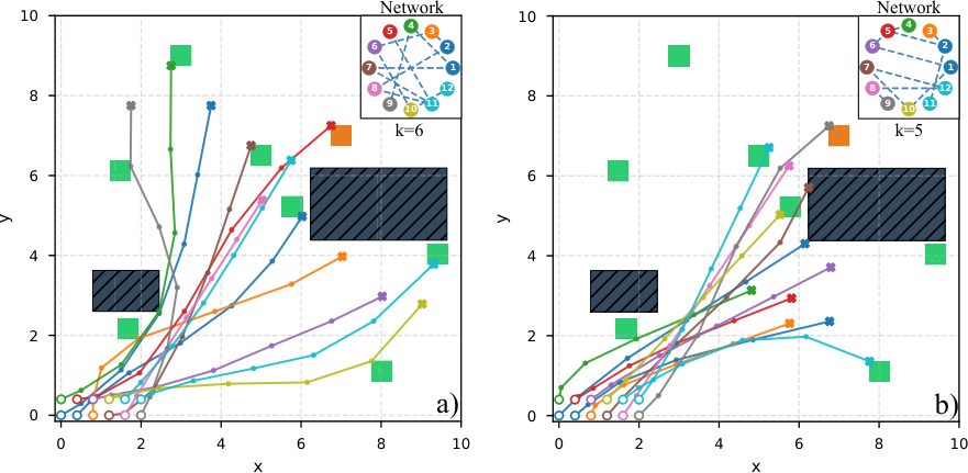
We divide the presentation of the results in two parts. First, an illustrative example comparing the flow and SEC approaches (Figure 2) for standard connectivity. Second, a statistical evaluation over 100 randomized scenarios with increasingly larger MAS (Table 3 and Figure 3).
In both cases, we consider a homogeneous MAS with agents’ dynamics represented by double integrators (sampling period second). The linear velocities were bounded to the interval and the corresponding accelerations to . The connectivity regions were modeled as squares of side 2. The optimization weights were chosen as and . The maximum planning horizon was set as . All problems were solved using the Gurobi optimizer 22 on a computer with an i5-1135G7 (2.4-4.2GHz) and 16GB RAM.
4.1 Networked MAS motion planning example
To illustrate the functionality of the proposed motion planning and decision-making algorithm, we employ the environment presented in Figure 2 for , which is based on the benchmark established in 18. For this particular example, the optimization time limit was selected as 600 seconds. Figure 2a shows the trajectories and target assignments considering the flow standard connectivity approach. The flow method enabled the MAS to reach each of the 7 optional targets in a maneuver of 6 seconds, whereas in the case of SEC (Figure 2b) only 4 optional targets were visited in a trajectory of 5 seconds. The connected communication network formed at the final step for each method is presented in the upper right corner of the corresponding figures, illustrating how the optimization enables the preservation of the communication by assigning some agents to the task of visiting targets while others serve as network relays. The final costs of the flow and SEC formulations were -69.9 and -41.7, respectively.
4.2 Randomized trials
We performed a statistical evaluation of the flow methods for standard and -hop connectivity considering randomized environments to compare their performance with the baselines SEC 18 and the matrix power method 40 for optimizations constrained to 60 seconds considering MAS with . The performance was assessed in terms of:
- a)
The rate of failure in finding a solution within the established time limit;
- b)
The quality of the best solution (if available) found within this time window;
- c)
The time required to compute the first feasible solution;
- d)
The first solution’s quality.
We note that items c) and d) are relevant metrics for receding horizon methods where feasible solutions must be computed in a relatively small time window.
The environments were generated with , . The positions of the obstacles and targets were determined using uniform distributions. Square obstacles with side were considered. In the -hop connectivity cases, the number of hops was selected as .
Table 3 presents the rate of failures considering the generated scenarios for each method and connectivity type as the number of agents in the MAS increases. We consider a model intractable if the rate of failure in finding solutions within the established time limit is greater than or equal to 50%. The results show that the SEC and flow formulations for standard connectivity yielded tractable models for and , respectively. Remarkably, we observe that the rate of failures almost doubles in the transition from 12 to 14 agents considering SEC, whereas the models under flow constraints presented a more controlled growth, indicating better scalability w.r.t. the size of the MAS.
| 4 | 6 | 8 | 10 | 12 | 14 | 16 | 18 | 20 | |
| Standard conn. | |||||||||
| SEC | 0 | 0 | 0 | 0 | 44 | 85 | 100 | 100 | 100 |
| Flow | 0 | 0 | 0 | 2 | 10 | 15 | 35 | 44 | 59 |
| 3-hop conn. | |||||||||
| Matrix power | 0 | 0 | 1 | 1 | 15 | 30 | 50 | – | – |
| Flow | 0 | 0 | 0 | 10 | 48 | 92 | 100 | – | – |
Figure 3 shows the statistical results. The data related to intractable cases (50% or more rate of failure) were omitted due to the insufficient samples. Figures 3a, 3b, and 3c, show that both methods performed similarly in all metrics for . However, the SEC formulation takes substantially more time to compute the first feasible solution than the flow for , and becomes intractable for larger MAS. The flow formulation consistently provides solutions within the time limit for . However, the variability in the value of the initial and final costs grows substantially for . Nevertheless, Figure 3c demonstrates that the solver is able to bring the final solutions to a cost between .
In the case of -hop connectivity, Table 3 shows that the matrix power and flow formulations provided tractable models for and , respectively. An approximated five-fold increase in the rate of failure was observed for the flow method in the transition from a model with to , which became intractable for . The existing matrix power formulation outperformed flow in terms of scalability, depicting a more controlled growth in the number of failures as the size of the MAS increases. Figure 3d illustrates the substantial time required to compute first solution under the flow scheme for . While the baseline generally performs better, we observe an approximate 6-fold growth in time for . Figures 3e demonstrate that for the flow method provides initial solutions with much more variance, being able to compute better first costs in a few instances, while the baseline consistently computes solutions with cost between around 10 and 100. However, 3f shows that the matrix power method provides much better capabilities of improving the initial solutions for .
4.3 Discussion
The results demonstrate that the flow encoding for standard connectivity provides substantial improvements in terms of scalability w.r.t. the size of the MAS, enabling the motion planning and decision-making problems to be solved for larger MAS within the established time limit compared to the SEC baseline. We attribute this result to the overall reduction in the scale of the MILP model provided by the flow formulation. The number of inequality constraints required by the SEC encoding grows exponentially with the number of agents, rendering the model intractable at moderate scales. In practice, the large number of constraints severely increases the time required by the solver’s presolve routines, which are a fundamental element of modern solvers, responsible for removing redundancies and tightening bounds. Indeed, for , the average presolve time under SEC was 28.2 seconds compared to 0.58 seconds under the flow formulation, indicating that nearly half of the allowed optimization time was spent in presolve in the case of SEC.
In the case of -hop connectivity, the main advantage of the proposed flow encoding is a substantial reduction in binary optimization variables, which dictate the worst-case number of iterations required by a branch-and-bound solver to find a global optimal solution. However, this reduction did not translate into practical performance gains within the imposed time limit. The overall increase in model size resulting from the additional continuous variables and inequality constraints resulted in worse scalability of the flow encoding compared to the matrix power baseline. In contrast to the standard connectivity case, the presolve times were comparable between the flow and matrix power formulations for -hop connectivity, suggesting that the performance gap originates from the cost of solving the LP relaxations at each branch-and-bound node. This is consistent with the growth of continuous variables and inequality constraints introduced by the flow encoding, which substantially increases the scale of the corresponding LP relaxations when compared to the matrix power baseline.
5 Conclusion
This work investigated the integration of connectivity maintenance constraints based on the concept of flow into \tl_set:NeMILP models used for motion planning and decision-making of \tl_set:NeMAS. We demonstrated that these alternative formulations encode necessary and sufficient conditions for standard and -hop connectivity, and evaluated their performance over the baselines using a statistical analysis over randomized trials for MAS of increasing sizes and a standard branch-and-bound commercial solver.
We conclude that the flow formulation is the most promising MILP implementation of standard connectivity constraints for networked MAS under branch-and-bound solve strategies. As such, future work should be directed at exploring methods to improve the scalability of these models, e.g., distributed MILP 9. Conversely, the flow formulation for -hop connectivity did not provide benefits over the baseline under restricted optimization times. However, we still see value in the reduction of binary variables provided by the flow implementation considering distinct solve strategies. In particular, we believe that methods based on decoupling the solution of binary and continuous variables can benefit substantially from this formulation. For example, deep reinforcement learning can be used to train a model to determine only the binary variables for a mixed-integer MPC controller 48. The reduced number of variables enables the use of smaller neural networks that can be efficiently trained and potentially provide better inference performance.
*Acknowledgments The authors have nothing to report.
*Funding This study was financed, in part, by the São Paulo Research Foundation (FAPESP), Brazil. Process Numbers 2024/04703-0 and 2025/01170-4.
*Disclosure The authors have nothing to report.
*Conflicts of Interest
The authors declare no conflicts of interest.
*Data availability statement The data that support the findings of this study are available from the corresponding author upon reasonable request.
References
- 1 Marco Dorigo, Guy Theraulaz, and Vito Trianni. Reflections on the future of swarm robotics. Science Robotics, 5(49):eabe4385, 2020.
- 2 Hamed Rezaee and Farzaneh Abdollahi. Average consensus over high-order multiagent systems. IEEE Transactions on Automatic Control, 60(11):3047–3052, 2015.
- 3 Michael Wooldridge. An introduction to multiagent systems. John wiley & sons, 2009.
- 4 Cecilia Garcia Cena, Pedro F. Cardenas, Roque Saltaren Pazmino, Lisandro Puglisi, and Rafael Aracil Santonja. A cooperative multi-agent robotics system: Design and modelling. Expert Systems with Applications, 40(12):4737–4748, 2013.
- 5 Jennifer Gielis, Ajay Shankar, and Amanda Prorok. A critical review of communications in multi-robot systems. Current robotics reports, 3(4):213–225, 2022.
- 6 Daniel Pickem, Paul Glotfelter, Li Wang, Mark Mote, Aaron Ames, Eric Feron, and Magnus Egerstedt. The robotarium: A remotely accessible swarm robotics research testbed. In 2017 IEEE International Conference on Robotics and Automation (ICRA), pages 1699–1706, 2017.
- 7 Tim Farnham, Simon Jones, Adnan Aijaz, Yichao Jin, Ioannis Mavromatis, Usman Raza, Anthony Portelli, Aleksandar Stanoev, and Mahesh Sooriyabandara. Umbrella collaborative robotics testbed and iot platform. In 2021 IEEE 18th Annual Consumer Communications & Networking Conference (CCNC), pages 1–7, 2021.
- 8 Wen Zhao, Mitsuhiro Kamezaki, Kaoru Yamaguchi, Minoru Konno, Akihiko Onuki, and Shigeki Sugano. A wheeled robot chain control system for underground facilities inspection using visible light communication and solar panel receivers. IEEE/ASME Transactions on Mechatronics, 27(1):180–189, 2022.
- 9 Andrea Testa, Guido Carnevale, and Giuseppe Notarstefano. A tutorial on distributed optimization for cooperative robotics: From setups and algorithms to toolboxes and research directions. Proceedings of the IEEE, 113(1):40–65, 2025.
- 10 Angelo Caregnato-Neto, Marcos ROA Maximo, and Rubens JM Afonso. Resilient robust connectivity for multiagent systems with line of sight using mixed-integer programming. Journal of Control, Automation and Electrical Systems, 33(1):129–140, 2022.
- 11 Chao Song, Xinyu Zhang, Yang She, Bo Li, and Qingfu Zhang. Trajectory planning for uav swarm tracking moving target based on an improved model predictive control fusion algorithm. IEEE Internet of Things Journal, 12(12):19354–19369, 2025.
- 12 Rudy R Negenborn, Bart De Schutter, and Johannes Hellendoorn. Multi-agent model predictive control: A survey. arXiv preprint arXiv:0908.1076, 2009.
- 13 Luigi D’Alfonso, Francesco Giannini, Giuseppe Franzè, Giuseppe Fedele, Francesco Pupo, and Giancarlo Fortino. Autonomous vehicle platoons in urban road networks: A joint distributed reinforcement learning and model predictive control approach. IEEE/CAA Journal of Automatica Sinica, 11(1):141–156, 2024.
- 14 Sungjun Seo and Kooktae Lee. On the convergence of density-based predictive control for multi-agent non-uniform area coverage. Journal of Dynamic Systems, Measurement, and Control, 148(2):021014, 01 2026.
- 15 Giuseppe Fedele and Giuseppe Franzè. A distributed model predictive control strategy for constrained multi-agent systems: The uncertain target capturing scenario. IEEE Transactions on Automation Science and Engineering, 21(2):1549–1563, 2023.
- 16 Francesca Pagano, Salvatore Marcellini, Mario Selvaggio, Vincenzo Lippiello, and Fabio Ruggiero. Multi-robot nonlinear model predictive control for persistent monitoring. IEEE Transactions on Control Systems Technology, 34(2):906–918, 2026.
- 17 Matthias Köhler, Matthias A. Müller, and Frank Allgöwer. Distributed mpc for self-organized cooperation of multiagent systems. IEEE Transactions on Automatic Control, 69(11):7988–7995, 2024.
- 18 Rubens J. M. Afonso, Marcos R. O. A. Maximo, and Roberto K. H. Galvao. Task allocation and trajectory planning for multiple agents in the presence of obstacle and connectivity constraint with mixed-integer linear programming. Int. J. Robust Nonlinear Control, 30(14):5464–5491, 9 2020.
- 19 Ignacio Sanchez, Agustina D’Jorge, Guilherme V Raffo, Alejandro H Gonzalez, and Antonio Ferramosca. Nonlinear model predictive path following controller with obstacle avoidance. Journal of Intelligent & Robotic Systems, 102(1):16, 2021.
- 20 Matthias Köhler, Matthias A. Müller, and Frank Allgöwer. Distributed model predictive control for dynamic cooperation of multi-agent systems, 2026.
- 21 A. Richards and J. How. Mixed-integer programming for control. In Proceedings of the 2005, American Control Conference, 2005., pages 2676–2683 vol. 4, 2005.
- 22 Gurobi Optimization, LLC. Gurobi Optimizer Reference Manual, 2025.
- 23 Daniel Ioan, Ionela Prodan, Sorin Olaru, Florin Stoican, and Silviu-Iulian Niculescu. Mixed-integer programming in motion planning. Annual Reviews in Control, 51:65–87, 2021.
- 24 Teodor Gabriel Crainic, Michel Gendreau, and Antonio Frangioni, editors. Combinatorial Optimization and Applications: A Tribute to Bernard Gendron. International Series in Operations Research & Management Science. Springer Cham, Cham, Switzerland, 2024. Edition 1.
- 25 Andrea Gasparri, Lorenzo Sabattini, and Giovanni Ulivi. Bounded control law for global connectivity maintenance in cooperative multirobot systems. IEEE Transactions on Robotics, 33(3):700–717, 2017.
- 26 Meng Ji and Magnus Egerstedt. Distributed coordination control of multiagent systems while preserving connectedness. IEEE Transactions on Robotics, 23(4):693–703, 2007.
- 27 Lorenzo Sabattini, Cristian Secchi, Nikhil Chopra, and Andrea Gasparri. Distributed control of multirobot systems with global connectivity maintenance. IEEE Transactions on Robotics, 29(5):1326–1332, 2013.
- 28 Alexandros Filotheou, Alexandros Nikou, and Dimos V Dimarogonas. Robust decentralised navigation of multi-agent systems with collision avoidance and connectivity maintenance using model predictive controllers. International Journal of Control, 93(6):1470–1484, 2020.
- 29 Andrea Simonetto, Tamás Keviczky, and Robert Babuška. Constrained distributed algebraic connectivity maximization in robotic networks. Automatica, 49(5):1348–1357, 2013.
- 30 Andrea Carron, Danilo Saccani, Lorenzo Fagiano, and Melanie N Zeilinger. Multi-agent distributed model predictive control with connectivity constraint. IFAC-PapersOnLine, 56(2):3806–3811, 2023.
- 31 Karlo Griparic, Marsela Polic, Marko Krizmancic, and Stjepan Bogdan. Consensus-based distributed connectivity control in multi-agent systems. IEEE Transactions on Network Science and Engineering, 9(3):1264–1281, 2022.
- 32 Hasan A. Poonawala and Mark W. Spong. Preserving strong connectivity in directed proximity graphs. IEEE Transactions on Automatic Control, 62(9):4392–4404, 2017.
- 33 Victoria Tuck, Yash Vardhan Pant, Sanjit A. Seshia, and S. Shankar Sastry. Dec-los-rrt: Decentralized path planning for multi-robot systems with line-of-sight constrained communication. In 2021 IEEE Conference on Control Technology and Applications (CCTA), pages 103–110, 2021.
- 34 Pham Q. Viet and Daniel Romero. Path planning for aerial relays via probabilistic roadmaps. IEEE Transactions on Communications, 74:4251–4266, 2026.
- 35 Tom Schouwenaars, Andrew Stubbs, James Paduano, and Eric Feron. Multivehicle path planning for nonline-of-sight communication. Journal of Field Robotics, 23(3-4):269–290, 2006.
- 36 Esten Ingar Grøtli and Tor Arne Johansen. Path planning for uavs under communication constraints using splat! and milp. Journal of Intelligent & Robotic Systems, 65(1):265–282, 2012.
- 37 Johan Thunberg and Petter Ögren. A mixed integer linear programming approach to pursuit evasion problems with optional connectivity constraints. Autonomous Robots, 31(4):333–343, 2011.
- 38 Pramod Abichandani, Hande Y. Benson, and Moshe Kam. Robust communication connectivity for multi-robot path coordination using mixed integer nonlinear programming: Formulation and feasibility analysis. In 2013 IEEE International Conference on Robotics and Automation, pages 3600–3605, 2013.
- 39 Pramod Abichandani, Solmaz Torabi, Shambadeb Basu, and Hande Benson. Mixed integer nonlinear programming framework for fixed path coordination of multiple underwater vehicles under acoustic communication constraints. IEEE Journal of Oceanic Engineering, 40(4):864–873, 2015.
- 40 Rubens J. M. Afonso, Roberto K. H. Galvão, Gabriel A. Souza, Marcos R. O. A. Maximo, and Angelo Caregnato-Neto. Linear constraints for ensuring k-hop connectivity using mixed-integer programming for multi-agent systems. International Journal of Robust and Nonlinear Control, 34(2):1433–1447, 2024.
- 41 Angelo Caregnato-Neto, Marcos R. O. A. Maximo, and Rubens J. M. Afonso. Mixed-integer motion planning for nonholonomic robots under visible light communication constraints. Optimal Control Applications and Methods, 46(3):1023–1035, 2025.
- 42 Jingjin Yu and Steven M LaValle. Multi-agent path planning and network flow. In Algorithmic Foundations of Robotics X: Proceedings of the Tenth Workshop on the Algorithmic Foundations of Robotics, pages 157–173. Springer, 2013.
- 43 Lishuo Pan, Kevin Hsu, and Nora Ayanian. Hierarchical large scale multirobot path (re) planning. In 2024 IEEE/RSJ International Conference on Intelligent Robots and Systems (IROS), pages 5319–5326. IEEE, 2024.
- 44 Emily M. Craparo, Jonathan P. How, and Eytan Modiano. Throughput optimization in mobile backbone networks. IEEE Transactions on Mobile Computing, 10(4):560–572, 2011.
- 45 Arthur Richards and Jonathan Pa How. Aircraft trajectory planning with collision avoidance using mixed integer linear programming. In in Proceedings of the 2002 American control conference (IEEE Cat. No. CH37301), pages 1936–1941, 2002.
- 46 V. Rodoplu and T.H. Meng. Minimum energy mobile wireless networks. IEEE Journal on Selected Areas in Communications, 17(8):1333–1344, 1999.
- 47 Luis Gouveia, Luigi Simonetti, and Eduardo Uchoa. Modeling hop-constrained and diameter-constrained minimum spanning tree problems as steiner tree problems over layered graphs, 2011.
- 48 Caio Fabio Oliveira da Silva, Azita Dabiri, and Bart De Schutter. Integrating reinforcement learning and model predictive control for mixed- logical dynamical systems. IEEE Open Journal of Control Systems, 4:316–331, 2025.
*