Envelopes of upper bounds for nonbinary constant-weight and constant-composition codes

Artur Akhiiarov Affiliation: Laboratory of Advanced Combinatorics and Network Applications, Moscow Institute of Physics and Technology (State University), Moscow, Russia Peter Boyvalenkov Affiliation: Institute of Mathematics and Informatics, Bulgarian Academy of Sciences, Sofia Danila Cherkashin Affiliation: Institute of Mathematics and Informatics, Bulgarian Academy of Sciences, Sofia Andrei Raigorodskii Affiliation: Department of Discrete Mathematics and Laboratory of Advanced Combinatorics and Network Applications, Moscow Institute of Physics and Technology (State University), Moscow, Russia Affiliation: Department of Mathematical Statistics and Random Processes, Faculty of Mechanics and Mathematics, Lomonosov Moscow State University, Moscow, Russia Affiliation: Caucasus Mathematical Center, Adyghe State University, Maykop, Republic of Adygea, Russia

September 2026

Abstract

Deriving upper bounds on code size from existing bounds is a classical approach in coding theory, dating back to the seminal results of Elias, Bassalygo, and Levenshtein. We study a framework encompassing the Bassalygo–Elias and Levenshtein inequalities for binary and nonbinary (constant-weight) codes and provides certain generalizations. The asymptotic cost of transferring a bound between different symbol compositions is expressed in terms of mutual information, yielding an information-theoretic optimal transport formulation.

We determine the optimal permutation-transport cost between arbitrary compositions in terms of their least common majorant in the majorization order. Specializing to symmetric constant-weight compositions yields explicit transport profiles. As a byproduct, we establish unimodality of the asymptotic constant-weight rate as a function of the relative weight. We prove that the resulting closure operators are idempotent and that applying transport before outer Bassalygo–Elias averaging leaves the unrestricted bound obtained from the same input unchanged. We also establish necessary and sufficient conditions for an upper bound to be a fixed point of the closure operator. Since the asymptotic rate function is an upper bound for itself and it is a fixed point, we conclude the Schur concavity of the constant-composition rate function.

Finally, we survey existing upper bounds for binary and nonbinary constant-weight and constant-composition codes, combine them into optimized envelopes within the transport framework, and obtain improved theoretical and numerical bounds.

1 Introduction

Fix an alphabet $\mathcal{A}$ with $|\mathcal{A}|=q$ , $q\geq 2$ is an integer, and a distinguished symbol $0$ . A code $C$ of length $n$ is any non-empty subset of $\mathcal{A}^{n}$ . A word $x$ is an element of $C$ . The weight of a word $x$ is the number $\wt(x)$ of non-zero symbols in $x$ . A constant-weight code with weight $w$ is a code in which every word has weight $w$ . Hamming distance $d_{H}(x,y)$ between words $x$ and $y$ is the number of positions in which $x$ and $y$ differ. The minimum distance $d(C)$ of a code $C$ is the smallest value of $d_{H}(x,y)$ over distinct $x,y\in C$ .

Two classical problems of coding theory consider the maximum possible cardinality of codes with fixed length and minimum distance and fixed length, constant weight, and minimum distance, respectively. Thus, we are interested in asymptotic upper bounds for the quantities

A_{q}(n,d):=\max\left\{|C|:C\subseteq\mathcal{A}^{n},\ d(C)\geq d\right\},

A_{q}(n,d,w):=\max\left\{|C|:C\subseteq\mathcal{A}^{n},\ \wt(x)=w\text{ for all }x\in C,\ d(C)\geq d\right\}.

We refer to the books [37, Chapter 17], [43, Chapters 5–7], [29, Chapters 1.9, 12, 13], [52, Chapter 3], and references therein from the enormous body of literature on the subject.

When considering codes as the length $n$ tends to infinity, one analyzes, respectively, the tradeoff between the relative minimum distance $d(C)/n\to\delta$ for $q$ -ary codes and asymptotic behavior of

R_{q}^{\mathrm{unr}}(\delta):=\limsup_{n\to\infty}\frac{1}{n}\log_{q}A_{q}(n,\lceil\delta n\rceil).

and between the relative weight $w/n\to\omega$ , the relative distance $d(C)/n\to\delta$ , and the asymptotic behavior of

R_{q}(\delta,\omega):=\limsup_{n\to\infty}\frac{1}{n}\log_{q}A_{q}(n,\lceil\delta n\rceil,\lceil\omega n\rceil)

for constant-weight codes (everywhere, $\delta,\omega\in[0,1]$ are real parameters).

We first derive a broad generalization of Levenshtein’s bound [34] from 1971. We prove two inequalities (Theorems 2.1 and 2.2) to provide transport between bounds for constant composition codes of the same distance. Setting a general framework, we derive an information-theoretic optimal transport formulation in which we find exact constant-composition transport cost (Theorem 3.2) and propose a plan for its “realization”. In the basic case, when both source and target are constant-weight, the problem is reduced to explicit computations leading to certain bounds (Corollary 3.5). Furthermore, the general framework allows us to define and investigate a closure operator which can be applied to all valid asymptotic upper bounds. We prove and study two major features of this operator, its idempotence (Theorem 4.1; i.e., one application is enough) and its majorization property (Proposition 4.2; explicitly showing that the constant-weight case provides optimality over the composition vectors). The majorization monotonicity gives, in particular, $q$ -ary unimodality of the asymptotic constant-composition rate which was previously considered only in the binary case [46, 15, 5]. The properties of an upper bound that cannot be improved at any source by our transport approach are investigated for obtaining necessary and sufficient conditions for unimprovability (Theorems 4.4 and 4.5). One of the main theoretical contributions of the paper (Corollary 4.6) shows that the constant-composition rate is Schur-concave.

Our general framework also allows unified treatment of all pre-existing bounds. This allows us to provide theoretical and numerical comparisons. Since not all known estimates have a simple description, a full explicit theoretical envelope looks difficult. Instead, some theoretical properties of the full envelope are provided in Section 6. They are based on the numerical observations which are discussed in Section 7.

Let us note that an immediate application of Levenshtein theorem from 1971 (inequality (6) below) to OpenAI moving subspace constant weight binary bound (see [41, Chapter 2, Lemma 3.5]) already gives some improvements. For instance, the upper bound on $R_{2}(0.1,0.2)$ changes from $0.42040\dots$ to $0.4145$ (see also Fig. 1). We provide examples (tables and graphs) of our refinements compared with best-known upper bounds for some values of the alphabet size $q$ .

The paper is organized as follows. In Section 2 we describe our main inequalities connecting upper bound for different regimes. Section 3 and 4 are devoted to theoretical analysis of these inequalities in the asymptotic regime. Then Section 5 collects known upper bounds which we combine with our approach theoretically in Section 6 and numerically in Section 7. Appendix A contains a relation of our optimal transport with the classical rate–distortion problem.

AI usage.

The authors used OpenAI ChatGPT Pro to refine the proofs, check calculations, and assist with manuscript preparation. All mathematical statements, proofs, computations, and citations were independently verified by the authors, who take full responsibility for the content of the manuscript.

Acknowledgments.

DC is supported by the Bulgarian National Science Fund Contract KP-06-N72/6-2023. PB is supported by the Ministry of Education and Science of Bulgaria under the Grant No. DO1-98/26.06.2025 “National Centre for High Performance and Distributed Computing” (NCHPDC). The authors would like to thank Alexander Barg for providing insightful remarks.

2 Main tools

We identify the alphabet $\mathcal{A}$ with the cyclic group $\mathbb{Z}_{q}$ . The composition vector of a word $c$ is the vector $(c_{0},\dots,c_{q-1})$ , where $c_{i}$ stands for the number of symbols $i$ in $c$ . A code $C$ is called constant-composition if all $x\in C$ have the same composition vector. If $C$ is constant-composition with a composition vector $\bm{w}$ , we write $\comp(C)=\bm{w}$ . For an integer composition vector $\bm{w}=(w_{a})_{a\in\mathcal{A}}$ with $\sum_{a}w_{a}=n$ , let

A_{q}(n,d;\bm{w}):=\max\bigl\{|C|:C\subseteq\mathcal{A}^{n},\ \comp(C)=\bm{w},\ d_{H}(x,y)\geq d\text{ for }x\neq y\bigr\}.

The quantity $A_{q}(n,d;\bm{w})$ is more general than the classical $A_{q}(n,d,w)$ and correspondingly allows more general treatment of the asymptotic bounds problem.

For a rational probability vector $p=(p_{a})_{a\in\mathcal{A}}$ and admissible integer sequences, write

R_{q}(\delta;p):=\limsup_{n\to\infty}\frac{1}{n}\log_{q}A_{q}(n,\lceil\delta n\rceil;np).

For the symmetric composition put $p_{\omega}:=\left(1-\omega,\frac{\omega}{q-1},\ldots,\frac{\omega}{q-1}\right)$ ; Proposition 4.2 below shows that $R_{q}(\delta,\omega)=R_{q}(\delta;p_{\omega})$ so the asymptotics of a constant-weight rate function coincides with the asymptotics of the corresponding symmetric composition.

Let $\tau=(\tau_{ab})_{a,b\in\mathbb{Z}_{q}}$ be a rational nonnegative $q\times q$ matrix of total mass one. We regard $\tau_{ab}$ as the proportion of coordinates on which the source symbol $a$ is sent to the target symbol $b$ . Denote by

p_{a}=\sum_{b\in\mathbb{Z}_{q}}\tau_{ab},\qquad r_{b}=\sum_{a\in\mathbb{Z}_{q}}\tau_{ab},

(1)

the row and column sums in the matrix $\tau$ , respectively. Thus $p=(p_{a})_{a\in\mathbb{Z}_{q}}$ and $r=(r_{b})_{b\in\mathbb{Z}_{q}}$ are the source and target compositions, respectively.

For $u\in\mathbb{Z}_{q}$ , define the distribution of the additive shift

\mu_{u}:=\sum_{a\in\mathbb{Z}_{q}}\tau_{a,a+u},

(2)

where the second index is taken modulo $q$ .

Our first main tool is the following theorem. Recall the definition of a multinomial coefficient

\binom{n}{v}:=\binom{n}{v_{1},\dots,v_{k}}=\frac{n!}{v_{1}!\cdot\dots\cdot v_{k}!},

where $v$ stands for the $k$ -tuple $(v_{1},\ldots,v_{k})$ with $v_{1}+\dots+v_{k}=n$ .

Theorem 2.1 (Transition-matrix transport inequality).

Let $p$ and $r$ be probability vectors and $\tau$ be a matrix with non-negative entries satisfying (1); assume that all $n\tau_{ab}$ are integers. Then, for every $n$ and $d$ ,

A_{q}(n,d;np)\leq\frac{\displaystyle\binom{n}{(n\mu_{u})_{u\in\mathbb{Z}_{q}}}}{\displaystyle\prod_{a\in\mathbb{Z}_{q}}\binom{np_{a}}{(n\tau_{ab})_{b\in\mathbb{Z}_{q}}}}A_{q}(n,d;nr).

(3)

Proof.

Let $C\subset\mathbb{Z}_{q}^{n}$ be a code of composition $np$ and size $A_{q}(n,d;np)$ . For each $x=(x_{1},\ldots,x_{n})\in C$ , consider all vectors $u=(u_{1},\ldots,u_{n})\in\mathbb{Z}_{q}^{n}$ , such that

\left|\{i:x_{i}=a,\ x_{i}+u_{i}=b\}\right|=n\tau_{ab}\ \ \mbox{for every}\ a,b\in\mathbb{Z}_{q}.

For a fixed $x$ , on the $np_{a}$ coordinates carrying the symbol $a$ , we choose which $n\tau_{ab}$ coordinates are sent to each $b\in\mathbb{Z}_{q}$ . Hence the number of admissible vectors $u$ is given by the product of multinomial coefficients

\prod_{a\in\mathbb{Z}_{q}}\binom{np_{a}}{(n\tau_{ab})_{b\in\mathbb{Z}_{q}}}.

If a coordinate undergoes the transition $a\mapsto b$ , then necessarily $u_{i}=b-a\pmod{q}$ .

Therefore every admissible $u$ has composition $n\mu$ , where $\mu$ is defined by (2). The total number of vectors in $\mathbb{Z}_{q}^{n}$ with this composition is

\binom{n}{(n\mu_{u})_{u\in\mathbb{Z}_{q}}}.

Now fix such a vector $u$ . The map

T_{u}:\mathbb{Z}_{q}^{n}\longrightarrow\mathbb{Z}_{q}^{n},\qquad T_{u}(x)=x+u

is a Hamming isometry. Moreover, for every pair $(x,u)$ counted above, the image $T_{u}(x)$ has composition $nr$ . Consequently, for a fixed $u$ , at most $A_{q}(n,d;nr)$ codewords of $C$ can occur in admissible pairs $(x,u)$ .

Double counting the admissible pairs $(x,u)$ therefore gives

|C|\prod_{a\in\mathbb{Z}_{q}}\binom{np_{a}}{(n\tau_{ab})_{b\in\mathbb{Z}_{q}}}\leq\binom{n}{(n\mu_{u})_{u\in\mathbb{Z}_{q}}}A_{q}(n,d;nr),

which is exactly (3), completing the proof. ∎

Theorem 2.1 uses only additive shifts in $\mathcal{A}$ . We prove the following extension (Theorem 2.2) to arbitrary coordinatewise permutations of $\mathcal{A}$ . For the symmetric source and target compositions analyzed below, the optimal information cost is already attained by additive shifts; see Proposition 3.7. The permutation extension is nevertheless essential for our proofs of majorization monotonicity and for the reduction of the fixed-weight problem to the balanced constant-composition problem, see Corollary 4.3 and Proposition 4.2.

Let $\mathcal{S}_{q}$ be the symmetric group on $\mathcal{A}$ . Let $\eta=(\eta_{a,\pi})_{a\in\mathcal{A},\pi\in\mathcal{S}_{q}}$ be a rational probability distribution ( $\eta$ is a counterpart of $\tau$ ). Write

p_{a}=\sum_{\pi}\eta_{a,\pi},\qquad\mu_{\pi}=\sum_{a}\eta_{a,\pi},\qquad r_{b}=\sum_{\begin{subarray}{c}a,\pi\\ \pi(a)=b\end{subarray}}\eta_{a,\pi}.

(4)

Theorem 2.2 (Permutation-transport inequality).

Let $p$ and $r$ be probability vectors and $\eta$ be a rational probability distribution satisfying (4); assume that all $n\eta_{a\pi}$ are integers.

A_{q}(n,d;np)\leq\frac{\displaystyle\binom{n}{(n\mu_{\pi})_{\pi\in\mathcal{S}_{q}}}}{\displaystyle\prod_{a\in\mathcal{A}}\binom{np_{a}}{(n\eta_{a,\pi})_{\pi\in\mathcal{S}_{q}}}}A_{q}(n,d;nr).

(5)

Proof.

Let $C\subset\mathcal{A}^{n}$ be a code with $\comp(C)=np$ and $|C|=A_{q}(n,d;np)$ . For each $x\in C$ , count all sequences $\bm{\pi}=(\pi_{1},\ldots,\pi_{n})\in\mathcal{S}_{q}^{n}$ such that

\left|\{i:x_{i}=a,\ \pi_{i}=\pi\}\right|=n\eta_{a,\pi}.

For fixed $x$ their number is the denominator in the ratio in (5). The total number of permutation sequences with marginal type $\mu=(\mu_{\pi})_{\pi\in\mathcal{S}_{q}}$ is the numerator. For a fixed $\bm{\pi}$ , the map

x\longmapsto\bm{\pi}(x):=(\pi_{1}(x_{1}),\ldots,\pi_{n}(x_{n}))

is a Hamming isometry, and every selected image has composition $nr$ . Consequently at most $A_{q}(n,d;nr)$ codewords can be paired with a fixed $\bm{\pi}$ . Double counting the pairs $(x,\bm{\pi})$ proves the claim. ∎

Restricting $\pi_{i}$ to the $q$ translations of a cyclic group recovers Theorem 2.1.

2.1 Levenshtein’s theorem revisited

Theorem 2.1 should be viewed as a nonbinary constant-composition generalization of the double-counting inequality used by Levenshtein [34] for binary constant-weight codes:

A_{2}(n,d,w)\leq\frac{\binom{n}{w-\beta+\alpha}}{\binom{n-w}{\alpha}\binom{w}{\beta}}A_{2}(n,d,\alpha+\beta),

(6)

where $\alpha\leq n-w$ and $\beta\leq w$ .

Indeed, for $q=2$ take the transition matrix

n\tau=\begin{pmatrix}n-w-\alpha&\alpha\\ w-\beta&\beta\end{pmatrix}.

Thus $\alpha$ zero coordinates are changed from $0$ to $1$ , $w-\beta$ one coordinates are changed from $1$ to $0$ , and the remaining coordinates are left unchanged. The target word therefore has weight $\alpha+\beta$ . The associated binary shift vector has weight $\alpha+(w-\beta)=w-\beta+\alpha$ . Hence Theorem 2.1 gives exactly (6).

2.2 Bassalygo averaging

We recall the averaging step that passes from a constant-weight bound to an unrestricted bound.

Lemma 2.3 (Bassalygo averaging).

For every $n,d,w$ ,

A_{q}(n,d)\leq\frac{q^{n}}{\binom{n}{w}(q-1)^{w}}\,A_{q}(n,d,w).

(7)

Proof.

Denote the shell of words of length $n$ and weight $w$ by $J_{q}(n,w)$ , i.e.

J_{q}(n,w):=\{x\in\mathcal{A}^{n}:\wt(x)=w\},\qquad|J_{q}(n,w)|=\binom{n}{w}(q-1)^{w}.

(8)

For an unrestricted code $C\subseteq\mathcal{A}^{n}$ of minimum distance at least $d$ and cardinality $A_{q}(n,d)$ , average $|(C+z)\cap J_{q}(n,w)|$ over $z\in\mathcal{A}^{n}$ . Every pair $(c,s)\in C\times J_{q}(n,w)$ determines a unique translation $z=s-c$ . Hence

\sum_{z\in\mathcal{A}^{n}}|(C+z)\cap J_{q}(n,w)|=|C|\cdot|J_{q}(n,w)|.

For some $z$ ,

|(C+z)\cap J_{q}(n,w)|\geq|C|\frac{|J_{q}(n,w)|}{q^{n}}.

Translation is a Hamming isometry, so this intersection is a constant-weight code of minimum distance at least $d$ . Therefore

|C|\frac{|J_{q}(n,w)|}{q^{n}}\leq A_{q}(n,d,w),

which proves (7). ∎

3 Asymptotic transport inequalities from Theorem 2.2

In this section we analyze how to apply Theorem 2.2 in the most effective way and justify the obtained asymptotic bounds. It is convenient to use the language of information-theoretic transport, with mutual information as the cost.

First, note that there are generally several transport plans $\eta$ with the same source and target marginals $p$ and $r$ . We determine the optimal permutation-transport cost between arbitrary compositions through their least common majorant, then specialize the result to the constant-weight case.

3.1 Entropy and mutual information

The definition of mutual information, the chain rule, and the data processing inequality are standard; see [16, Sections 2.3–2.8] and [17, Chapter 2]. All random variables considered here take values in finite sets, and all logarithms are to base $q$ . For the historical origin of these notions, see [48].

For a probability distribution $P$ on a set $\mathcal{S}$ , define

H_{q}(P):=-\sum_{x\in\mathcal{S}}P(x)\log_{q}P(x).

For a random variable $X$ with distribution $P_{X}$ , write $H_{q}(X):=H_{q}(P_{X})$ . Then define the $q$ -ary entropy function

h_{q}(x):=-x\log_{q}x-(1-x)\log_{q}(1-x)+x\log_{q}(q-1).

We use the convention $0\log 0=0$ . Thus $H_{q}(p_{\omega})=h_{q}(\omega)$ , where $p_{\omega}$ is the constant-composition vector $\left(1-\omega,\frac{\omega}{q-1},\ldots,\frac{\omega}{q-1}\right)$ .

Conditional entropy and mutual information.

For two random variables $X,Y$ , write $H_{q}(X,Y):=H_{q}(P_{XY})$ . Their conditional entropy is

H_{q}(X\mid Y):=\sum_{y:\,P_{Y}(y)>0}P_{Y}(y)\,H_{q}(P_{X\mid Y=y}),\qquad P_{X\mid Y=y}(x):=\frac{P_{XY}(x,y)}{P_{Y}(y)}.

Thus $H_{q}(X\mid Y)$ is the average entropy of the conditional distributions. Conditioning on several variables means conditioning on their tuple, for example $H_{q}(X\mid Y,Z):=H_{q}(X\mid(Y,Z))$ .

The chain rule for entropy states that

H_{q}(X,Y)=H_{q}(Y)+H_{q}(X\mid Y).

Its conditional form is

H_{q}(X,Y\mid Z)=H_{q}(X\mid Z)+H_{q}(Y\mid X,Z).

Let $X$ and $Y$ be random variables with joint distribution $P_{XY}$ and marginals $P_{X}$ and $P_{Y}$ . Their mutual information is defined by

I_{q}(X;Y):=\sum_{x,y}P_{XY}(x,y)\log_{q}\frac{P_{XY}(x,y)}{P_{X}(x)P_{Y}(y)}.

Equivalently,

I_{q}(X;Y)=H_{q}(X)-H_{q}(X\mid Y)=H_{q}(Y)-H_{q}(Y\mid X)=H_{q}(X)+H_{q}(Y)-H_{q}(X,Y).

Terms with $P_{XY}(x,y)=0$ contribute zero. Moreover, $I_{q}(X;Y)\geq 0$ , and $I_{q}(X;Y)=0$ if and only if $X$ and $Y$ are independent.

Conditional mutual information and the chain rule.

For random variables $X,Y,Z$ , define

I_{q}(X;Y\mid Z):=H_{q}(X\mid Z)-H_{q}(X\mid Y,Z)=H_{q}(Y\mid Z)-H_{q}(Y\mid X,Z).

It is nonnegative, with equality exactly when $X$ and $Y$ are conditionally independent given $Z$ , meaning that

P_{XY\mid Z=z}(x,y)=P_{X\mid Z=z}(x)P_{Y\mid Z=z}(y)

for every $z$ of positive probability.

The chain rule for mutual information is

I_{q}(X;Y,Z)=I_{q}(X;Y)+I_{q}(X;Z\mid Y)=I_{q}(X;Z)+I_{q}(X;Y\mid Z).

Here $I_{q}(X;Y,Z)$ denotes mutual information between $X$ and the pair $(Y,Z)$ . Nonnegativity of conditional mutual information also gives

H_{q}(X\mid Y,Z)\leq H_{q}(X\mid Y)\leq H_{q}(X).

Data processing inequality.

We write $X\to Y\to Z$ when $X$ and $Z$ are conditionally independent given $Y$ . Equivalently, their joint distribution factorizes as

P_{XYZ}(x,y,z)=P_{X}(x)P_{Y\mid X=x}(y)P_{Z\mid Y=y}(z);

which is called the Markov-chain condition.

The data-processing inequality states that

I_{q}(X;Z)\leq I_{q}(X;Y)\qquad\text{for}\qquad X\to Y\to Z.

(9)

In particular, $I_{q}(X;f(Y))\leq I_{q}(X;Y)$ for every deterministic function $f$ , with equality when $f$ is bijective.

Convexity in the channel.

For a fixed input distribution $p$ , mutual information is convex in the conditional distribution of the output [16, Theorem 2.7.4]. Explicitly, let $X\sim p$ , and let $P_{Y_{i}\mid X}=W_{i}$ , $i=1,2$ , be channels with the same input and output alphabets. If

P_{Y\mid X}=\lambda W_{1}+(1-\lambda)W_{2},\qquad 0\leq\lambda\leq 1,

then

I_{q}(X;Y)\leq\lambda I_{q}(X;Y_{1})+(1-\lambda)I_{q}(X;Y_{2}).

The same statement holds for any finite convex combination of channels.

Majorization and Schur concavity.

We say that a nonincreasing probability vector $y$ majorizes nonincreasing probability vector $x$ , and write $x\preceq y$ when

\sum_{i=1}^{j}x_{i}\leq\sum_{i=1}^{j}y_{i}\quad(1\leq j<k),

where $k$ is the length of $x$ and $y$ . A permutation-invariant function $f$ on probability vectors of length $k$ is Schur-concave if $f(x)\geq f(y)$ provided that $x\preceq y$ . Entropy function $H_{q}$ is strictly Schur-concave, which means that $H_{q}(x)=H_{q}(y)$ and $x\preceq y$ imply $x=y$ . Also, it is concave in the usual sense, that is

H_{q}(\lambda p_{1}+(1-\lambda)p_{2})\geq\lambda H_{q}(p_{1})+(1-\lambda)H_{q}(p_{2})

for all probability vectors $p_{1},p_{2}$ and $0\leq\lambda\leq 1$ .

3.2 Asymptotic case of Theorem 2.2

The passage from Theorem 2.2 to an asymptotic rate is a standard method-of-types calculation [18]: multinomial coefficients become entropies, and a quotient of conditional and marginal type-class sizes becomes a mutual information; see, for example, [11, 16]. This observation is particularly useful here because it turns the combinatorial choice of an auxiliary permutation sequence into a finite-dimensional information-theoretic optimization.

Let $\Pi$ be a random variable on the symmetric group $\mathcal{S}_{q}$ , let $(X,\Pi)$ have joint distribution $\eta$ , and let $Y=\Pi(X)$ . Stirling’s formula applied to (5) gives the following form of Theorem 2.2. As usual, we write $X\sim Z$ for equidistributed random variables $X$ and $Z$ .

Corollary 3.1.

For every joint distribution of $(X,\Pi)$ with $X\sim p$ and $Y=\Pi(X)\sim r$ ,

R_{q}(\delta;p)\leq I_{q}(X;\Pi)+R_{q}(\delta;r),

(10)

where $I_{q}$ denotes mutual information measured in base- $q$ units.

Indeed, the exponent of the multinomial ratio is $H_{q}(\Pi)-H_{q}(\Pi\mid X)=I_{q}(X;\Pi)$ .

Relation with conditional-type Elias arguments.

The appearance of mutual information in (10) is not specific to the permutation formulation. It is the standard exponential loss in conditional-type versions of the Bassalygo–Elias argument. Indeed, Blahut’s composition bounds [11] are formulated using stochastic matrices subject to mutual-information constraints. In a particularly transparent modern formulation, Dalai’s conditional-composition covering lemma [19, Lemma 3] shows that a constant-composition code $C$ contains a subcode $C^{\prime}$ of size

|C^{\prime}|\geq|C|\,q^{-n(I_{q}(P,V)+o(1))}

whose codewords have a prescribed joint type with a fixed auxiliary composition. Here $I_{q}(P,V)=I_{q}(X;U)$ , where $X\sim P$ and $U\mid X=x\sim V(\cdot\mid x)$ . The finite permutation inequality used here gives an exact group-action realization of the same conditional-type mechanism.

We shall continue investigation of the relations of our approach with the Bassalygo–Elias argument in Subsection 6.2.

3.3 Optimal transport between arbitrary compositions

The permutation inequality (10) also permits a target whose nonzero symbol frequencies are not equal. Introduce the minimal transport cost as

K_{q}(p,r):=\min_{P_{\Pi\mid X}:\,\Pi(X)\sim r}I_{q}(X;\Pi),\qquad X\sim p,\quad\Pi\in\mathcal{S}_{q}.

(11)

Thus the strongest form of (10) becomes $R_{q}(\delta;p)\leq K_{q}(p,r)+R_{q}(\delta;r)$ . The minimum in (11) is attained, since the feasible set of joint distributions is compact and mutual information is continuous. The next result (Theorem 3.2) solves (11) and thus eliminates optimization over the permutation-valued auxiliary variable $\Pi$ .

For a vector $v$ define $v^{\downarrow}$ as the permuted vector whose entries go in the non-increasing order. We say that a probability vector $s$ majorizes a probability vector $p$ if $p^{\downarrow}\preceq s^{\downarrow}$ . From combinatorial point of view the coordinates order in the composition vector does not matter, so we will simply write $p\preceq s$ . Majorization gives a standard partial order on probability vectors. Denote the least common majorant of vectors $p$ and $r$ in the corresponding lattice by $p^{\downarrow}\vee r^{\downarrow}$ . The majorization lattice and its entropy functionals have been studied in [14, 13]. In particular, the symmetric quantity

\mathsf{d}_{q}(p,r):=H_{q}(p)+H_{q}(r)-2H_{q}(p^{\downarrow}\vee r^{\downarrow})

(12)

defines a metric on nonincreasing probability vectors.

For a permutation $\sigma\in\mathcal{S}_{q}$ and a probability vector $v$ , write $(\sigma(v))_{x}:=v_{\sigma^{-1}(x)}$ . Thus, if $S\sim v$ , then $\sigma(S)$ has distribution $\sigma(v)$ . We use the standard characterization of majorization:

u\preceq v\quad\Longleftrightarrow\quad u\in\operatorname{conv}\{\sigma(v):\sigma\in\mathcal{S}_{q}\}.

(13)

This follows from the doubly stochastic characterization of majorization and the Birkhoff–von Neumann theorem; see [38, Chapters 2 and 4].

Theorem 3.2 (Exact constant-composition transport cost).

Let $p,r$ be probability vectors on the $q$ -letter alphabet $\mathcal{A}$ , and put $s:=p^{\downarrow}\vee r^{\downarrow}$ . Then

K_{q}(p,r)=H_{q}(p)-H_{q}(s).

(14)

Moreover, let

p=\sum_{i}\alpha_{i}\sigma_{i}(s),\qquad r=\sum_{j}\beta_{j}\rho_{j}(s),

where $\sigma_{i},\rho_{j}\in\mathcal{S}_{q}$ , $\alpha_{i},\beta_{j}\geq 0$ , and $\sum_{i}\alpha_{i}=\sum_{j}\beta_{j}=1$ , be arbitrary convex representations of $p$ and $r$ (such representations exist because $p,r\preceq s$ ). Then an optimal joint distribution of $(X,\Pi)$ is

\Pr\{X=x,\Pi=\pi\}=\sum_{i,j:\,\rho_{j}\circ\sigma_{i}^{-1}=\pi}\alpha_{i}\beta_{j}s_{\sigma_{i}^{-1}(x)}.

(15)

Proof.

Consider any feasible joint distribution of $(X,\Pi)$ , with $X\sim p$ and $Y=\Pi(X)\sim r$ . Put $\mu_{\pi}:=\Pr\{\Pi=\pi\}$ . For each $\pi$ with $\mu_{\pi}>0$ , define

v_{a,\pi}:=\Pr\{X=a\mid\Pi=\pi\},\qquad v_{\pi}:=(v_{a,\pi})_{a\in\mathcal{A}}.

Then, for every $a,b\in\mathcal{A}$ ,

p_{a}=\Pr\{X=a\}=\sum_{\pi\in\mathcal{S}_{q}}\mu_{\pi}v_{a,\pi},\qquad r_{b}=\Pr\{Y=b\}=\sum_{\begin{subarray}{c}a\in\mathcal{A},\;\pi\in\mathcal{S}_{q}\\ \pi(a)=b\end{subarray}}\mu_{\pi}v_{a,\pi},

and

H_{q}(X\mid\Pi)=-\sum_{\pi\in\mathcal{S}_{q}}\mu_{\pi}\sum_{a\in\mathcal{A}}v_{a,\pi}\log_{q}v_{a,\pi}=\sum_{\pi\in\mathcal{S}_{q}}\mu_{\pi}H_{q}(v_{\pi}).

Set

s_{0}:=\sum_{\pi}\mu_{\pi}v_{\pi}^{\downarrow}.

This is a non-increasing probability vector. For each $k$ , the function $F_{k}(v):=\sum_{i=1}^{k}v_{i}^{\downarrow}$ is convex, since it is the maximum of the sums of $k$ coordinates. Therefore

F_{k}(p)\leq\sum_{\pi}\mu_{\pi}F_{k}(v_{\pi})=F_{k}(s_{0}).

The same argument applied to the mixture defining $r$ , together with $F_{k}(\pi(v_{\pi}))=F_{k}(v_{\pi})$ , gives $F_{k}(r)\leq F_{k}(s_{0})$ . Thus $p,r\preceq s_{0}$ , and the defining property of the join implies $s\preceq s_{0}$ .

By concavity and Schur concavity of entropy,

H_{q}(X\mid\Pi)=\sum_{\pi}\mu_{\pi}H_{q}((v_{\pi})^{\downarrow})\leq H_{q}(s_{0})\leq H_{q}(s).

Hence every feasible transport satisfies $I_{q}(X;\Pi)\geq H_{q}(p)-H_{q}(s)$ .

For the reverse inequality, take convex representations from (13). Let $S,I,J$ be mutually independent, with

\Pr\{S=x\}=s_{x},\qquad\Pr\{I=i\}=\alpha_{i},\qquad\Pr\{J=j\}=\beta_{j},

and define

X:=\sigma_{I}(S),\qquad\Pi:=\rho_{J}\circ\sigma_{I}^{-1},\qquad Y:=\Pi(X)=\rho_{J}(S).

The two convex representations give $X\sim p$ and $Y\sim r$ . This construction induces exactly the joint distribution stated above.

Since $\Pi$ is a deterministic function of $(I,J)$ , data processing inequality (9) gives $I_{q}(X;\Pi)\leq I_{q}(X;I,J)$ . Conditionally on $I=i,J=j$ , the distribution of $X$ is $\sigma_{i}(s)$ , whose entropy is $H_{q}(s)$ . Consequently,

I_{q}(X;\Pi)\leq H_{q}(p)-H_{q}(X\mid I,J)=H_{q}(p)-H_{q}(s).

Together with the lower bound, this proves the formula and the optimality of the constructed plan. ∎

The least-concave-majorant algorithm.

Here we present a standard algorithm to find $s=p^{\downarrow}\vee r^{\downarrow}$ for given $p$ and $r$ . The algorithm is linear in $q$ after the sorting (which has complexity $O(q\log q)$ ).

Set $m_{0}=0$ , $m_{q}=1$ , and

m_{k}=\max\left\{\sum_{i=1}^{k}p_{i}^{\downarrow},\sum_{i=1}^{k}r_{i}^{\downarrow}\right\}.

Start with the increments $m_{k}-m_{k-1}$ as unit-length blocks. Whenever two adjacent block slopes increase, merge the blocks and replace their slopes by their length-weighted average. Continue until the block slopes are nonincreasing. This gives the least concave majorant $\widehat{m}$ of the polygonal line through $(k,m_{k})$ . The join has coordinates $s_{i}=\widehat{m}(i)-\widehat{m}(i-1)$ . Once the join and the two convex decompositions have been computed, the realizing plan is given by (15).

For $q=3$ the least common majorant can be written explicitly. Let $M$ and $m$ be the maximum and the minimum among all entries of $p$ and $r$ , respectively. Then

p^{\downarrow}\vee r^{\downarrow}=(M,1-M-m,m),\qquad K_{3}(p,r)=H_{3}(p)-H_{3}(M,1-M-m,m).

Indeed, the largest coordinate of any common majorant is at least $M$ , and its smallest coordinate is at most $m$ . The vector $p^{\downarrow}\vee r^{\downarrow}$ is non-increasing and satisfies both requirements.

Corollary 3.3.

The cost (14) is zero exactly when $r\preceq p$ . Also, $K_{q}(p,r)=H_{q}(p)-H_{q}(r)$ if and only if $p\preceq r$ .

3.4 Optimal transport between constant-weight layers

In the next section (Proposition 4.2) we shall prove that from the asymptotic point of view the constant-weight case coincides with the symmetric composition case $p_{t}=\left(1-t,\frac{t}{q-1},\ldots,\frac{t}{q-1}\right)$ for $0\leq t\leq 1$ . Now we study the optimal transport between symmetric source and target.

Recall that the preceding least-concave-majorant algorithm computes the transport cost. For symmetric compositions, the computation is particularly simple and can be done explicitly. For $1\leq k\leq q-1$ , the sum of the $k$ largest components of $p_{t}$ is

P_{k}(t):=\sum_{i=1}^{k}(p_{t}^{\downarrow})_{i}=\begin{cases}1-t+\dfrac{(k-1)t}{q-1},&0\leq t\leq(q-1)/q,\\[5.69054pt] \dfrac{kt}{q-1},&(q-1)/q\leq t\leq 1.\end{cases}

(16)

The algorithm is applied to $\max\{P_{k}(\omega),P_{k}(\theta)\}$ , with the endpoint values $0$ and $1$ . Once the join is known, an optimal transport plan is obtained by the construction in Theorem 3.2.

We call the intervals on which the profile has the explicit expressions below its branches; the first branch is the one adjacent to $\theta=0$ . The branches can now be determined by comparing the partial sums in (16) and pooling their slopes as in the least-concave-majorant algorithm.

The terminology for the first branch comes from Fano’s inequality [16, Section 2.10], see (17) below. For a feasible transport with $X\sim p_{\omega}$ and $\Pi(X)\sim p_{\theta}$ , put $Z:=\Pi^{-1}(0)$ . Then $Z\in\mathcal{A}$ , $\Pr\{X\neq Z\}=\theta$ , and data processing inequality (9) gives $I_{q}(X;Z)\leq I_{q}(X;\Pi)$ . If $E=\mathbf{1}_{\{X\neq Z\}}$ and $\Pr\{E=1\}=\theta$ , then

H_{q}(X\mid Z)=H_{q}(E\mid Z)+H_{q}(X\mid E,Z)\leq H_{q}(E)+\theta\log_{q}(q-1)=h_{q}(\theta).

Indeed, when $E=0$ , the value of $X$ is determined by $Z$ , whereas when $E=1$ , at most $q-1$ possibilities remain. Therefore

I_{q}(X;Z)\geq h_{q}(\omega)-h_{q}(\theta),\qquad X\sim p_{\omega}.

(17)

The next proposition gives a compact expression for the entire profile. The following Corollary 3.5 identifies its branches explicitly. In particular, it shows that Fano’s lower bound is sharp on the initial interval, see (21) below.

Proposition 3.4 (Complete constant-weight profile).

Let $q\geq 3$ and $\omega,\theta\in[0,1]$ . Put

M:=\max\left\{1-\omega,1-\theta,\frac{\omega}{q-1},\frac{\theta}{q-1}\right\},\quad\ell:=\min\left\{1-\omega,1-\theta,\frac{\omega}{q-1},\frac{\theta}{q-1}\right\},

(18)

and $\lambda:=(1-M-\ell)/(q-2)$ . Then

p_{\omega}^{\downarrow}\vee p_{\theta}^{\downarrow}=\left(M,\underbrace{\lambda,\ldots,\lambda}_{q-2\text{ entries}},\ell\right),

(19)

and consequently

K_{q}(p_{\omega},p_{\theta})=h_{q}(\omega)+M\log_{q}M+(q-2)\lambda\log_{q}\lambda+\ell\log_{q}\ell.

(20)

Proof.

For $t\in\{\omega,\theta\}$ , let $P_{k}(t)$ be as defined in (16). Clearly, these partial sums are linear in $k$ on $1\leq k\leq q-1$ , regardless of which side of $(q-1)/q$ contains $t$ . Moreover,

M=\max\{P_{1}(\omega),P_{1}(\theta)\},\qquad 1-\ell=\max\{P_{q-1}(\omega),P_{q-1}(\theta)\}.

We compute the least concave majorant directly.

A composition attaining the smallest component $\ell$ has all its other components at most $M$ , while a composition attaining the largest component $M$ has all its other components at least $\ell$ . Thus $1-\ell\leq(q-1)M$ and $1-M\geq(q-1)\ell$ . These inequalities give

M\geq\lambda\geq\ell\geq 0,

so $s=(M,\lambda,\ldots,\lambda,\ell)$ is a non-increasing probability vector. Its partial sums are

S_{k}=M+(k-1)\lambda=\frac{q-1-k}{q-2}M+\frac{k-1}{q-2}(1-\ell),\qquad 1\leq k\leq q-1.

Since each $P_{k}(t)$ is linear in $k$ and its two endpoint values are bounded above by $M$ and $1-\ell$ , respectively,

P_{k}(\omega)\leq S_{k},\qquad P_{k}(\theta)\leq S_{k}.

Hence $s$ majorizes both compositions.

Conversely, let $u=(u_{0},\dots,u_{q-1})$ be any non-increasing common majorant of $p_{\omega}$ and $p_{\theta}$ . Denote by $U_{k}$ , $1\leq k\leq q$ , the partial sums of $u$ . Then $U_{1}\geq M$ and $U_{q-1}\geq 1-\ell$ . This and the concavity of its partial sums imply

U_{k}\geq\frac{q-1-k}{q-2}U_{1}+\frac{k-1}{q-2}U_{q-1}\geq S_{k},\qquad 1\leq k\leq q-1.

Therefore $s\preceq u$ , proving (19). Theorem 3.2 now gives (20) thus completing the proof. ∎

Inspecting the cases in (18) gives the following explicit representation of Proposition 3.4.

Corollary 3.5.

For $\omega>0$ and $q\geq 3$ , put $t_{0}=(q-1)(1-\omega)$ , $t_{1}=1-\frac{\omega}{q-1}$ , $t_{2}=\omega$ , and define

\bar{h}_{q-1}^{(q)}(z):=-z\log_{q}z-(1-z)\log_{q}(1-z)+z\log_{q}(q-2),\qquad 0\leq z\leq 1.

Then the complete profile is

K_{q}(p_{\omega},p_{\theta})=\begin{cases}h_{q}(\omega)-h_{q}(\theta),&\begin{array}[]{@{}l@{}}\theta\leq\min\{t_{0},t_{2}\}\\[-2.84526pt] \text{or }\theta\geq\max\{t_{0},t_{2}\},\end{array}\\[8.53581pt] 0,&\min\{t_{1},t_{2}\}\leq\theta\leq\max\{t_{1},t_{2}\},\\[5.69054pt] \displaystyle\omega\left[\log_{q}(q-1)-\bar{h}_{q-1}^{(q)}\!\left(\frac{\theta-1+\omega}{\omega}\right)\right],&\text{otherwise}.\end{cases}

(21)

All cases are restricted to $\theta\in[0,1]$ , and the expressions agree at common endpoints. If $t_{0}>1$ , the condition $\theta\geq\max\{t_{0},t_{2}\}$ gives an empty branch. For $\omega=0$ , and any $\theta$ one has $K_{q}(p_{0},p_{\theta})=0$ .

Proof.

To obtain the piecewise expression, the same partial-sum comparison gives

	$\displaystyle p_{\omega}\preceq p_{\theta}$	$\displaystyle\quad\Longleftrightarrow\quad\theta\leq\min\{t_{0},t_{2}\}\ \text{or}\ \theta\geq\max\{t_{0},t_{2}\},$
	$\displaystyle p_{\theta}\preceq p_{\omega}$	$\displaystyle\quad\Longleftrightarrow\quad\min\{t_{1},t_{2}\}\leq\theta\leq\max\{t_{1},t_{2}\}.$

In these two regimes the join is, respectively, $p_{\theta}^{\downarrow}$ and $p_{\omega}^{\downarrow}$ , giving the first and second expressions in (21).

In every remaining case the compositions are incomparable, and Proposition 3.4 implies that their join is a permutation of $(1-\omega,1-\theta,u,\dots,u)$ , with $u:=(\omega+\theta-1)/(q-2)$ appearing $q-2$ times. Put $z:=(\theta-1+\omega)/\omega$ . Here $0\leq z\leq 1$ , and the same vector can be written, up to permutation, as $(1-\omega,\omega(1-z),\omega z/(q-2),\ldots,\omega z/(q-2))$ .

Recall that $s=p_{\omega}^{\downarrow}\vee p_{\theta}^{\downarrow}$ ; splitting off the mass $1-\omega$ in the entropy yields

H_{q}(p_{\omega})-H_{q}(s)=\omega\left[\log_{q}(q-1)-\bar{h}_{q-1}^{(q)}(z)\right],

which proves the remaining expression. At the boundaries the respective join vectors coincide, so the formulas agree. Finally, when $\omega=0$ , the join is $(1,0,\ldots,0)$ ; hence (20) gives zero. ∎

The ordering of the branches in (21) depends on the source weight $\omega$ . For $\omega>(q-1)/q$ , one has $t_{0}<t_{1}<t_{2}$ , and the incomparable regime “otherwise” lies before the zero-information interval. For $0<\omega<(q-1)/q$ , the order is $t_{2}<t_{1}<t_{0}$ , and the incomparable regime lies after that interval. The former is the classical reverse-water-filling regime; the latter belongs to the positive exact-distortion continuation beyond the zero-information interval (see Appendix A). At $\omega=(q-1)/q$ , for any $\theta$ the three thresholds coincide and

K_{q}(p_{(q-1)/q},p_{\theta})=1-h_{q}(\theta).

Remark 3.6.

In the case $q=2$ , the two compositions are always comparable in the majorization order, and

K_{2}(p_{\omega},p_{\theta})=\max\{h_{2}(\omega)-h_{2}(\theta),0\}.

In the following proposition we verify that if both source and target compositions are symmetric then Theorem 2.2 cannot asymptotically refine Theorem 2.1.

Proposition 3.7.

For symmetric compositions $p_{\omega},p_{\theta}$ , an optimal permutation transport can also be realized by additive shifts of $\mathbb{Z}_{q}$ .

Proof.

For $q=2$ , every alphabet permutation is an additive shift, so assume $q\geq 3$ . Choose an optimal permutation transport $(X,\Pi)$ from $p_{\omega}$ to $p_{\theta}$ , as provided by Theorem 3.2, and put $Z:=\Pi^{-1}(0)$ . Since $X=Z$ if and only if $\Pi(X)=0$ , data processing inequality (9) gives

\Pr\{X=Z\}=1-\theta,\qquad I_{q}(X;Z)\leq I_{q}(X;\Pi)=K_{q}(p_{\omega},p_{\theta}).

Average the joint distribution of $(X,Z)$ under simultaneous alphabet permutations fixing $0$ , and denote the resulting pair by $(X^{\prime},Z^{\prime})$ . These relabelings preserve the source distribution $p_{\omega}$ and the event of equality. By invariance under bijective relabeling and convexity of mutual information in the channel for a fixed source distribution,

X^{\prime}\sim p_{\omega},\qquad\Pr\{X^{\prime}=Z^{\prime}\}=1-\theta,\qquad I_{q}(X^{\prime};Z^{\prime})\leq K_{q}(p_{\omega},p_{\theta}).

Write $Q_{xz}:=\Pr\{X^{\prime}=x,Z^{\prime}=z\}$ . By symmetry, there are constants $A,B,C$ such that

Q_{0j}=A,\qquad Q_{i0}=B,\qquad Q_{ij}=C\quad(i,j\neq 0,\ i\neq j).

For every $u\neq 0$ , subtraction in $\mathbb{Z}_{q}$ gives

\Pr\{X^{\prime}-Z^{\prime}=u\}=\sum_{z\in\mathbb{Z}_{q}}Q_{z+u,z}=A+B+(q-2)C.

Thus all nonzero differences have the same probability. Since $\Pr\{X^{\prime}-Z^{\prime}=0\}=1-\theta$ , we obtain $X^{\prime}-Z^{\prime}\sim p_{\theta}$ . Then the random translation $x\mapsto x-Z^{\prime}$ is a feasible permutation transport.

Consequently,

K_{q}(p_{\omega},p_{\theta})\leq I_{q}(X^{\prime};-Z^{\prime})=I_{q}(X^{\prime};Z^{\prime})\leq K_{q}(p_{\omega},p_{\theta}).

Hence the additive transport is optimal. ∎

4 The closure operator and its properties

In this section we define the closure operator, investigate its idempotence and prove necessary, and sufficient conditions on fixed points of the operator.

Let $\Delta_{q-1}$ denote the probability simplex on $\mathcal{A}$ , that is the convex hull of standard basis vectors in $\mathbb{R}^{q}$ . Let $B_{q}(\delta;r)$ be a valid asymptotic upper bound for every composition $r$ . Define the constant-composition closure operator

(\mathcal{P}B_{q})(\delta;p):=\inf_{r\in\Delta_{q-1}}\{K_{q}(p,r)+B_{q}(\delta;r)\}.

Theorem 3.2 has already optimized the information cost of transferring a bound between two prescribed compositions. Thus the remaining optimization is over the target composition $r$ alone:

(\mathcal{P}B_{q})(\delta;p)=H_{q}(p)+\inf_{r\in\Delta_{q-1}}\{B_{q}(\delta;r)-H_{q}(p^{\downarrow}\vee r^{\downarrow})\}.

4.1 Idempotence and majorization

The following theorem follows from a certain triangle-type inequality and implies that no finite chain of intermediate compositions improves a single application of the presented method.

Theorem 4.1 (Idempotence).

The constant-composition closure operator is idempotent, that is for every upper bound $B_{q}$ we have

\mathcal{P}(\mathcal{P}B_{q})=\mathcal{P}B_{q}.

Proof.

We first prove that, for any compositions $p,r,s$ ,

K_{q}(p,s)\leq K_{q}(p,r)+K_{q}(r,s).

(22)

Choose optimal transports $X\stackrel{{\scriptstyle\Pi}}{{\longmapsto}}Y$ and $Y\stackrel{{\scriptstyle\Sigma}}{{\longmapsto}}Z$ , with respective marginals $p,r,s$ . Realize the second transport so that $\Sigma$ is conditionally independent of $(X,\Pi)$ given $Y$ , and put $\Theta=\Sigma\circ\Pi$ . The chain rule and data processing inequality (9) give

I_{q}(X;\Theta)\leq I_{q}(X;\Pi,\Sigma)=I_{q}(X;\Pi)+I_{q}(X;\Sigma\mid\Pi)=

=I_{q}(X;\Pi)+I_{q}(Y;\Sigma\mid\Pi)\leq I_{q}(X;\Pi)+I_{q}(Y;\Sigma).

Here we used the conditional bijection $Y=\Pi(X)$ , the fact that $H_{q}(\Sigma\mid\Pi)\leq H_{q}(\Sigma)$ and $H_{q}(\Sigma\mid Y,\Pi)=H_{q}(\Sigma\mid Y)$ . Since $\Theta$ transports $p$ to $s$ , this proves (22).

Consequently,

	$\displaystyle(\mathcal{P}(\mathcal{P}B_{q}))(\delta;p)$	$\displaystyle=\inf_{r,s\in\Delta_{q-1}}\{K_{q}(p,r)+K_{q}(r,s)+B_{q}(\delta;s)\}$
		$\displaystyle\geq\inf_{s\in\Delta_{q-1}}\{K_{q}(p,s)+B_{q}(\delta;s)\}=(\mathcal{P}B_{q})(\delta;p).$

Choosing $r=p$ gives the reverse inequality. ∎

Proposition 4.2 (Uniform nonzero composition).

For every $\omega$ ,

R_{q}(\delta;p_{\omega})=R_{q}(\delta,\omega).

Proof.

For any composition vector $p=(1-\omega,p_{1},\ldots,p_{q-1})$ choose $\Pi$ , independently of $X$ , uniformly from the subgroup $\mathcal{S}_{q-1}\leq\mathcal{S}_{q}$ of permutations with fixed $0$ . Then

I_{q}(X;\Pi)=0\qquad\text{ and }\qquad\Pi(X)\sim p_{\omega}.

Corollary 3.1 gives $R_{q}(\delta;p)\leq R_{q}(\delta;p_{\omega})$ uniformly over all source compositions of weight $\omega$ .

By inclusion, we have

A_{q}(n,d,w)\leq\sum_{\wt(\bm{w})=w}A_{q}(n,d,\bm{w}).

Since the number of summands is polynomial in $n$ , passing to the limit gives

R_{q}(\delta,\omega)\leq\max_{p,p_{1}+\dots+p_{q-1}=\omega}R_{q}(\delta;p)=R_{q}(\delta;p_{\omega}).

The inverse inequality is obvious by inclusion. ∎

Now we are in a position to show that $R_{q}(\delta,\omega)$ is unimodal in $\omega$ , i.e. for every fixed $\delta$ function $R_{q}(\delta,\omega)$ increases before $\omega=(q-1)/q$ and decreases later. In fact, Corollary 4.6 gives a stronger result of the behavior of $R_{q}(\delta,\omega)$ . In the binary case, the unimodality results were obtained by Samorodnitsky [46], see also [5].

Corollary 4.3 (Majorization monotonicity).

If $r\preceq p$ , then

R_{q}(\delta;p)\leq R_{q}(\delta;r).

(23)

Thus the asymptotic constant-composition rate is Schur-concave. In particular, for fixed $\delta$ , the function $\omega\mapsto R_{q}(\delta,\omega)$ is nondecreasing on $[0,(q-1)/q]$ and nonincreasing on $[(q-1)/q,1]$ .

Proof.

Since $r\preceq p$ , Corollary 3.3 gives $K_{q}(p,r)=0$ . The asymptotic transport inequality (10) therefore yields (23).

Writing $\omega_{*}=(q-1)/q$ , comparison of partial sums 16 gives $p_{\omega_{2}}\preceq p_{\omega_{1}}$ for $0\leq\omega_{1}\leq\omega_{2}\leq\omega_{*}$ and $p_{\omega_{1}}\preceq p_{\omega_{2}}$ for $\omega_{*}\leq\omega_{1}\leq\omega_{2}\leq 1$ . The stated weight monotonicity follows, using Proposition 4.2 for the passage from symmetric compositions to full constant-weight shells. ∎

4.2 Bounds unchanged by permutation transport

Throughout this subsection, $q\geq 2$ and $\delta\in[0,1]$ are fixed. We characterize finite-valued upper bounds that cannot be improved at any source by the permutation-transport operator. The criteria are pointwise in $\delta$ and impose no relation between different distances.

We will use the metric $\mathsf{d}_{q}(p,r)$ , defined in (12), on compositions modulo coordinate permutations.

Theorem 4.4 (Unimprovable composition-dependent bounds).

Let $B_{q}(\delta;\cdot)$ be an upper bound on $R_{q}(\delta;\cdot)$ . The following conditions are equivalent.

1.

For every $p\in\Delta_{q-1}$ ,

$(\mathcal{P}B_{q})(\delta;p)=B_{q}(\delta;p).$
2.

Both functions

$p\longmapsto B_{q}(\delta;p),\qquad p\longmapsto H_{q}(p)-B_{q}(\delta;p)$

are Schur-concave.
3.

For every $p\preceq r$ ,

$0\leq B_{q}(\delta;p)-B_{q}(\delta;r)\leq H_{q}(p)-H_{q}(r).$ (24)

For every $p,r\in\Delta_{q-1}$ ,

\left|\bigl(2B_{q}(\delta;p)-H_{q}(p)\bigr)-\bigl(2B_{q}(\delta;r)-H_{q}(r)\bigr)\right|\leq\mathsf{d}_{q}(p,r).

(25)

Proof.

Since $K_{q}(p,p)=0$ , condition 1 is equivalent to the family of inequalities

B_{q}(\delta;p)-B_{q}(\delta;r)\leq K_{q}(p,r)\qquad(p,r\in\Delta_{q-1}).

(26)

Indeed, these inequalities give $B\leq\mathcal{P}B$ , whereas the diagonal choice $r=p$ always gives $\mathcal{P}B\leq B$ .

If $p\preceq r$ , the join formula yields

K_{q}(p,r)=H_{q}(p)-H_{q}(r),\qquad K_{q}(r,p)=0.

Applying (26) in both directions proves (24). Conditions 2 and 3 are equivalent by the definition of Schur-concavity. Notice that mutually majorizing vectors give equality in (24), so permutation invariance is also a consequence of condition 3.

Conversely, assume condition 3. For arbitrary $p,r$ , put $s=p^{\downarrow}\vee r^{\downarrow}$ . Since $p,r\preceq s$ ,

B_{q}(\delta;p)-B_{q}(\delta;r)\leq B_{q}(\delta;p)-B_{q}(\delta;s)\leq H_{q}(p)-H_{q}(s)=K_{q}(p,r).

Thus (26) holds and condition 1 follows.

Finally,

2K_{q}(p,r)=\mathsf{d}_{q}(p,r)+H_{q}(p)-H_{q}(r).

Consequently, the two directed inequalities for $(p,r)$ and $(r,p)$ in (26) are equivalent to (25), that is condition 4. ∎

For a constant-weight input bound $B_{q}(\delta,\theta)$ we use the extension $B_{q}(\delta;r)=B_{q}(\delta,1-r_{0})$ , where $r_{0}$ is the first coordinate of $r$ . At a symmetric source the closure is

(\mathcal{P}B_{q})(\delta;p_{\omega})=\inf_{0\leq\theta\leq 1}\{K_{q}(p_{\omega},p_{\theta})+B_{q}(\delta,\theta)\}.

(27)

Thus unimprovability of a weight-only bound means equality in (27) with $B_{q}(\delta,\omega)$ for every $\omega$ . It concerns the symmetric sources $p_{\omega}$ ; it does not assert that the extension $r\mapsto B_{q}(\delta,1-r_{0})$ is a fixed point on the entire simplex.

Theorem 4.5 (Unimprovable weight-dependent bounds).

Let $B_{q}(\delta,\cdot)$ be an upper bound on $R_{q}(\delta,\cdot)$ , and put

f(\omega)=B_{q}(\delta,\omega),\qquad h(\omega)=h_{q}(\omega).

The bound is unchanged by (27) at every weight if and only if

\left|2f(x)-h(x)-2f(y)+h(y)\right|\leq\mathsf{d}_{q}(p_{x},p_{y})\qquad(0\leq x,y\leq 1).

(28)

For $q>2$ , an equivalent explicit criterion consists of the following two sets of conditions.

(a) Within each branch:

	$\displaystyle 0\leq f(y)-f(x)$	$\displaystyle\leq h(y)-h(x),$		$\displaystyle 0\leq x\leq y\leq\frac{q-1}{q},$		(29)
	$\displaystyle 0\leq f(x)-f(y)$	$\displaystyle\leq h(x)-h(y),$		$\displaystyle\frac{q-1}{q}\leq x\leq y\leq 1.$		(30)

(b) Between the branches: for $0\leq x\leq(q-1)/q\leq y\leq 1$ , put

a_{y}=(q-1)(1-y),\qquad b_{y}=1-\frac{y}{q-1}.

Then

	$\displaystyle 0\leq f(y)-f(x)$	$\displaystyle\leq h(y)-h(x),$		$\displaystyle x\leq a_{y},$		(31)
	$\displaystyle 0\leq f(x)-f(y)$	$\displaystyle\leq h(x)-h(y),$		$\displaystyle x\geq b_{y}.$		(32)

For $a_{y}<x<b_{y}$ , define as in (19)

s_{x,y}=\left(1-x,\underbrace{\frac{x+y-1}{q-2},\ldots,\frac{x+y-1}{q-2}}_{q-2\text{ entries}},1-y\right).

The remaining condition is

H_{q}(s_{x,y})-h(y)\leq f(x)-f(y)\leq h(x)-H_{q}(s_{x,y}).

(33)

Proof.

As in (26), unimprovability is equivalent to

f(x)-f(y)\leq K_{q}(p_{x},p_{y})\qquad(0\leq x,y\leq 1).

(34)

Combining the inequalities in both directions gives (28).

On each side of $(q-1)/q$ , the symmetric compositions form a majorization chain. Specifically,

p_{y}\preceq p_{x}:\quad 0\leq x\leq y\leq\frac{q-1}{q},\qquad p_{x}\preceq p_{y}:\quad\frac{q-1}{q}\leq x\leq y\leq 1.

The comparable-pair costs therefore give (29)–(30).

Suppose $q>2$ and $x\leq(q-1)/q\leq y$ . The partial sums of the sorted compositions, for $1\leq k\leq q-1$ , are

P_{k}=1-x+\frac{(k-1)x}{q-1},\qquad Q_{k}=\frac{ky}{q-1}.

Their difference is affine in $k$ . Comparing its values at $k=1$ and $k=q-1$ gives

p_{y}\preceq p_{x}\iff x\leq a_{y},\qquad p_{x}\preceq p_{y}\iff x\geq b_{y}.

These cases yield (31) and (32). In the remaining case $a_{y}<x<b_{y}$ , we have $p_{x}^{\downarrow}\vee p_{y}^{\downarrow}=s_{x,y}$ by Proposition 3.4.

The two directions of (34) now give (33). At $x=a_{y}$ or $x=b_{y}$ the join reduces to the appropriate comparable composition. All pairs have been covered, proving necessity and sufficiency of (a)–(b). ∎

Conditions (29)–(30) say that both $f$ and its entropy deficit $h_{q}-f$ are nondecreasing up to $(q-1)/q$ and nonincreasing thereafter. For $q>2$ , the full criterion also includes (31)–(33): the symmetric one-parameter family is not closed under taking joins.

Corollary 4.6 (Structural properties of the exact asymptotic rates).

For every fixed $q\geq 2$ and $\delta\in[0,1]$ , the following hold.

1.

The exact constant-composition rate is a fixed point: $(\mathcal{P}R_{q})(\delta;p)=R_{q}(\delta;p)$ . Both $R_{q}(\delta;\cdot)$ and $H_{q}-R_{q}(\delta;\cdot)$ are Schur-concave. In particular,

$0\leq R_{q}(\delta;p)-R_{q}(\delta;r)\leq H_{q}(p)-H_{q}(r)\qquad(p\preceq r).$ (35)
2.

The exact constant-weight rate is also unchanged by weight transport:

$R_{q}(\delta,\omega)=\inf_{0\leq\theta\leq 1}\{K_{q}(p_{\omega},p_{\theta})+R_{q}(\delta,\theta)\}.$

It satisfies all the conditions of Theorem 4.5. In particular, both functions $\omega\longmapsto R_{q}(\delta,\omega)$ and $\omega\longmapsto h_{q}(\omega)-R_{q}(\delta,\omega)$ are nondecreasing on $[0,(q-1)/q]$ and nonincreasing on $[(q-1)/q,1]$ .

The function $f(\omega)=R_{q}(\delta,\omega)$ is absolutely continuous on $[0,1]$ , and almost everywhere

\begin{cases}0\leq f^{\prime}(\omega)\leq\displaystyle\log_{q}\frac{(q-1)(1-\omega)}{\omega},&0<\omega<\frac{q-1}{q},\\[5.69054pt] \displaystyle\log_{q}\frac{(q-1)(1-\omega)}{\omega}\leq f^{\prime}(\omega)\leq 0,&\frac{q-1}{q}<\omega<1.\end{cases}

(36)

4.

With $u_{q}=(1/q,\ldots,1/q)$ ,

$0\leq R_{q}(\delta;u_{q})-R_{q}(\delta;p)\leq 1-H_{q}(p).$ (37)

Consequently,

$0\leq f\left(\frac{q-1}{q}\right)-f(\omega)\leq 1-h_{q}(\omega),\qquad f^{\prime}\left(\frac{q-1}{q}\right)=0.$ (38)

The derivative at $(q-1)/q$ exists without any additional regularity assumption.

Proof.

Corollary 3.1 and Theorem 3.2 give directly

R_{q}(\delta;p)\leq K_{q}(p,r)+R_{q}(\delta;r)\qquad(p,r\in\Delta_{q-1}).

Taking the infimum over $r$ , and using $r=p$ for the reverse inequality, proves the first fixed-point identity. Theorem 4.4 then gives the Schur-concavity assertions and (35). Restricting to $p=p_{\omega}$ , $r=p_{\theta}$ , and applying Proposition 4.2 proves the second fixed-point identity. Theorem 4.5 gives the stated monotonicities and all cross-branch inequalities.

On either closed branch, the increment inequalities imply

|f(y)-f(x)|\leq|h_{q}(y)-h_{q}(x)|.

Since $h_{q}$ is absolutely continuous and monotone on each branch, the definition of absolute continuity, applied to disjoint intervals, shows that $f$ is absolutely continuous there as well. The two restrictions agree at $(q-1)/q$ , so $f$ is absolutely continuous on $[0,1]$ . Differentiating the increment inequalities at points where $f^{\prime}$ exists gives (36), since

h_{q}^{\prime}(\omega)=\log_{q}\frac{(q-1)(1-\omega)}{\omega}.

Finally, $u_{q}\preceq p$ for every $p$ , so (35) implies (37). Taking $p=p_{\omega}$ gives the inequality in (38). The Taylor expansion

1-h_{q}(\omega)=\frac{q^{2}}{2(q-1)\ln q}\left(\omega-\frac{q-1}{q}\right)^{2}+O\left(\left|\omega-\frac{q-1}{q}\right|^{3}\right)

then proves $f^{\prime}((q-1)/q)=0$ . ∎

The binary case.

For $q=2$ , the complete criterion for $f=B_{2}(\delta,\omega)$ instead takes the form

f(\omega)=F(h_{2}(\omega)),\qquad 0\leq\omega\leq 1,

(39)

where $F:[0,1]\to\mathbb{R}$ is nondecreasing and $1$ -Lipschitz.

Indeed, $p_{\omega}$ and $p_{1-\omega}$ differ only by a coordinate permutation. Their costs in both directions are zero, so $f(\omega)=f(1-\omega)$ is necessary. The compositions on $[0,1/2]$ form a chain, and $h_{2}$ maps that interval continuously and strictly increasingly onto $[0,1]$ . Its inverse defines $F$ in (39); the lower-branch increment inequalities are exactly

0\leq F(t)-F(s)\leq t-s\qquad(0\leq s\leq t\leq 1).

Conversely, these inequalities and the symmetry implied by (39) give (34) for every pair.

The monotonicity of $R_{2}(\delta,\omega)$ and of $h_{2}(\omega)-R_{2}(\delta,\omega)$ on $[0,1/2]$ is classical. Both assertions are stated explicitly in Samorodnitsky [46, Section 4, Lemmas 4.1–4.2], with attribution to Levenshtein’s work.

5 Base bounds to which the closure operator is applied

This section describes weight-dependent and unrestricted asymptotic upper bounds. We shall collect bounds $B_{q}(\delta,\theta)$ , suitably abbreviated, which will serve as input for the closure operator $\mathcal{P}$ . The purpose of the section is broader than the preparation to the final numerical comparison. A bound is omitted from the latter envelope whenever it is contained pointwise in a kept family, or when no closed proportional-parameter evaluation is presently available.

5.1 Shell size, shell balls, and Plotkin–Johnson

The shell $J_{q}(n,w)$ (see (8)) itself has exponent $h_{q}(\omega)$ . The asymptotic form of the unrestricted Singleton bound gives the additional elementary ceiling $R_{q}(\delta,\omega)\leq 1-\delta$ . Neither the shell-size ceiling nor the Singleton ceiling is used in the final comparison: on its domain each is no stronger than the kept families.

For $q\geq 3$ , let $\alpha,\beta\geq 0$ satisfy $\alpha\leq 1-\omega$ , $\alpha+\beta\leq\omega$ , and put $\gamma=\omega-\alpha-\beta$ . Define

\Phi_{q}^{\mathrm{rel}}(\omega;\alpha,\beta):=(1-\omega)h_{q}\left(\frac{\alpha}{1-\omega}\right)+\omega H_{q}\left(\frac{\alpha}{\omega},\frac{\beta}{\omega},\frac{\gamma}{\omega}\right)+\beta\log_{q}(q-2).

This is the exponent of the $(\alpha,\beta)$ -relation in $\mathcal{A}^{n}$ with respect to a fixed word of weight $\omega n$ . Hence the shell-ball exponent is,

V_{q}(\rho,\omega)=\max_{\mathcal{D}}\Phi_{q}^{\mathrm{rel}}(\omega;\alpha,\beta),

(40)

where the optimization domain $\mathcal{D}$ contains $\alpha,\beta\geq 0$ such that $\alpha\leq 1-\omega$ , $\alpha+\beta\leq\omega$ , and $2\alpha+\beta\leq\rho$ . Then the shell Hamming bound is

B_{q}^{\mathrm{Ham}}(\delta,\omega)=h_{q}(\omega)-V_{q}(\delta/2,\omega).

For $q=2$ the corresponding formulas are obtained from the binary Johnson scheme and should be written separately rather than by substituting $q=2$ into $\Phi_{q}^{\mathrm{rel}}(\omega;\alpha,\beta)$ .

The above Hamming–Johnson construction belongs to the relation-layer Bassalygo–Elias bound envelope, which we consider below, so adding the shell-Hamming curve cannot lower the selected envelope.

The asymptotic average-distance threshold [31, 34] in the symmetric constant-weight shell is

\delta_{q}^{\mathrm{Pl}}(\omega)=1-(1-\omega)^{2}-\frac{\omega^{2}}{q-1}=2\omega-\frac{q}{q-1}\omega^{2}.

Therefore

B^{\mathrm{Pl}}_{q}(\delta,\omega)=R_{q}(\delta,\omega)=0\qquad\text{for}\qquad\delta\geq\delta_{q}^{\mathrm{Pl}}(\omega).

(41)

The zero-rate region of this Plotkin bound is already enforced by the following relation-layer Bassalygo–Elias bound.

5.2 Relation-layer Bassalygo–Elias bound

For $q\geq 3$ , define

\delta_{q}^{\mathrm{loc}}(\omega;\alpha,\beta):=2\alpha-\frac{q\alpha^{2}}{(q-1)(1-\omega)}+\omega-\frac{\alpha^{2}+\gamma^{2}+\beta^{2}/(q-2)}{\omega},\qquad\gamma=\omega-\alpha-\beta.

Averaging over a relation layer and applying Plotkin’s bound inside the selected subcode gives

B_{q}^{\mathrm{rel-BE}}(\delta,\omega)=h_{q}(\omega)-\sup_{\begin{subarray}{c}\alpha,\beta\geq 0\\ \alpha\leq 1-\omega,\ \alpha+\beta\leq\omega\\ \delta_{q}^{\mathrm{loc}}(\omega;\alpha,\beta)\leq\delta\end{subarray}}\Phi_{q}^{\mathrm{rel}}(\omega;\alpha,\beta).

(42)

This family gives best-known bounds for some values of parameters and so we keep it in the final envelope.

5.3 Code–anticode bounds

The code–anticode principle provides a second general way of converting diametric information inside a shell $J_{q}(n,w)$ into an upper bound. Let

I_{q}(n,D,w):=\max\{|A|:A\subset J_{q}(n,w),\diam(A)\leq D\}.

For a vertex transitive graph $G=(V,E)$ the folklore clique-coclique bound (see, for instance, [28]) gives

\alpha(G)\cdot\omega(G)\leq|V(G)|.

(43)

Now let $G$ be a graph with the vertex set $J_{q}(n,w)$ and whose edges connect pairs of vertices at the Hamming distance at most $d-1$ . Clearly $G$ is vertex transitive, so (43) gives

A_{q}(n,d,w)\cdot I_{q}(n,d-1,w)\leq|J_{q}(n,w)|=\binom{n}{w}(q-1)^{w}.

(44)

In particular, every explicit anticode gives a valid upper bound, whether or not it is known to be maximum.

Binary constant-weight codes.

For $q=2$ , write $s:=\left\lfloor(d-1)/2\right\rfloor$ and $t:=w-s$ . An anticode of Hamming diameter at most $2s$ is the same as a $t$ -intersecting family of $w$ -subsets. The complete intersection theorem of Ahlswede and Khachatrian [2] determines its maximum cardinality:

I_{2}(n,2s,w)=\max_{i}\sum_{j=t+i}^{\min\{w,t+2i\}}\binom{t+2i}{j}\binom{n-t-2i}{w-j},

(45)

where

0\leq i\leq\min\left\{w-t,\left\lfloor\frac{n-t}{2}\right\rfloor\right\},\qquad w\leq n/2,\qquad 0\leq s\leq w.

Consequently

A_{2}(n,d,w)\leq\frac{\binom{n}{w}}{I_{2}(n,2\lfloor(d-1)/2\rfloor,w)}.

For numerical asymptotics one may apply Stirling’s formula directly to (45). Assuming $0\leq\omega\leq 1/2$ (the other half follows by complementation) and $0\leq\delta\leq 2\omega$ , put $\tau_{0}:=\omega-\delta/2$ . Then the anticode exponent is

\alpha_{2}^{\mathrm{AK}}(\delta,\omega):=\sup_{\mathcal{D}}\left((\tau_{0}+2\iota)h_{2}\!\left(\frac{x}{\tau_{0}+2\iota}\right)+(1-\tau_{0}-2\iota)h_{2}\!\left(\frac{\omega-x}{1-\tau_{0}-2\iota}\right)\right),

where the optimization is over $(x,\iota)\in\mathcal{D}$ defined by $0\leq\iota\leq\min\{\delta/2,(1-\tau_{0})/2\}$ , $x\geq\tau_{0}+\iota$ , $x\leq\min\{\omega,\tau_{0}+2\iota\}$ and $\omega-x\leq 1-\tau_{0}-2\iota$ . Hence the complete-intersection code–anticode bound in the binary case is

B_{2}^{\mathrm{CA}}(\delta,\omega)=h_{2}(\omega)-\alpha_{2}^{\mathrm{AK}}(\delta,\omega).

This binary complete-intersection curve is recorded here because of its theoretical importance. It is covered by the moving-subspace Johnson-layer construction appearing below.

Nonbinary constant-weight codes.

For $q>2$ , the code–anticode inequality (44) is available, but the maximum anticode size is not known for all proportional parameters. Etzion [24] identifies several families of maximum anticodes for special parameter ranges and leaves the general diametric problem open. Two explicit families were nevertheless used asymptotically.

First, fix the support of the word and allow $D$ specified nonzero coordinates to vary over $\mathcal{A}\setminus\{0\}$ , while fixing the remaining nonzero symbols. This gives an anticode of diameter at most $D$ and size $(q-1)^{D}$ . Second, fix $\tau n$ coordinates to one prescribed nonzero symbol and allow the remaining $(1-\tau)n$ coordinates to run through $J_{q}((1-\tau)n,(\omega-\tau)n)$ . Its exponent is

a_{q}^{\mathrm{s}}(\tau,\omega)=(1-\tau)h_{q}\!\left(\frac{\omega-\tau}{1-\tau}\right)

and its Hamming diameter has relative value at most $d_{q}^{\mathrm{s}}(\tau,\omega)=\min\{2(\omega-\tau),\,1-\tau\}$ . Thus an available anticode exponent is

\alpha_{q}^{\mathrm{ex}}(\delta,\omega):=\max\left\{\min\{\delta,\omega\}\log_{q}(q-1),\ \sup_{\begin{subarray}{c}0\leq\tau\leq\omega\\ d_{q}^{\mathrm{s}}(\tau,\omega)<\delta\end{subarray}}a_{q}^{\mathrm{s}}(\tau,\omega)\right\}

yielding the bound

B_{q}^{\mathrm{CA,ex}}(\delta,\omega):=h_{q}(\omega)-\alpha_{q}^{\mathrm{ex}}(\delta,\omega),\qquad q>2.

The superscript “ex” here means that the bound follows from a particular anticode example: unlike the binary complete-intersection expression where the diametric problem has been solved.

The explicit nonbinary code–anticode bound is covered by the $B_{q}^{cc-CA}$ bound.

For the unrestricted Hamming space, the maximum-anticode problem is known exactly by the diametric theorem of Ahlswede and Khachatrian [3]. This underlies, in particular, the optimal-anticode refinements used in nonbinary unrestricted bounds such as Kaipa’s [32].

5.4 The Ben-Haim–Litsyn product-scheme bound

We use the finite-dimensional asymptotic formulation of Ben-Haim and Litsyn [9]. As written below, the formulas require $q\geq 3$ ; boundary values are understood by continuity. Define

k_{q}(x)=\frac{q-1}{q}-\frac{q-2}{q}x-\frac{2}{q}\sqrt{(q-1)x(1-x)},\qquad h(x,y)=\frac{x(1-x)-y(1-y)}{1+2\sqrt{y(1-y)}}.

Put

R_{1}(q,\omega,\delta):=\min_{\mathcal{D}_{1}}\biggl\{h_{q}(\xi)+\xi h_{q}\!\left(\frac{\eta}{\xi}\right)-(\xi+\eta)\log_{q}(q-1)+\eta\log_{q}(q-2)\biggr\},

where the optimization domain $\mathcal{D}_{1}\ni(\eta,\xi)$ is defined by inequalities

0\leq\eta\leq\frac{q-2}{q-1}\omega,\qquad 0\leq\xi-\eta\leq\min\{\omega-\eta,1-\omega\},

b=(1-\eta)h\!\left(\frac{\omega-\eta}{1-\eta},\frac{\xi-\eta}{1-\eta}\right)\leq\omega-\frac{q-1}{q-2}\eta,\qquad\delta\geq 2b+(\omega-b)k_{q-1}\!\left(\frac{\eta}{\omega-b}\right).

Next define

R_{2}(q,\omega,\nu,\phi,\delta):=\min_{\mathcal{D}_{2}}\biggl\{\nu R_{1}\!\left(q,\frac{\phi}{\nu},\delta_{1}\right)+(1-\nu)R_{1}\!\left(q,\frac{\omega-\phi}{1-\nu},\delta_{2}\right)\biggr\},

where the domain $\mathcal{D}_{2}\ni(\delta_{1},\delta_{2})$ is defined by $\nu\delta_{1}+(1-\nu)\delta_{2}=\delta$ , $0\leq\delta_{1}\leq\min\{2\phi/\nu,1\}$ , $0\leq\delta_{2}\leq\min\{2(\omega-\phi)/(1-\nu),1\}$ . Finally, the Ben-Haim–Litsyn upper bound on $R_{q}(\delta,\omega)$ is

B_{q}^{\mathrm{BHL}}(\delta,\omega):=\min_{\begin{subarray}{c}0\leq\phi\leq\nu\\ 0\leq\omega-\phi\leq 1-\nu\end{subarray}}\biggl\{h_{q}(\omega)-\nu h_{q}\!\left(\frac{\phi}{\nu}\right)-(1-\nu)h_{q}\!\left(\frac{\omega-\phi}{1-\nu}\right)+R_{2}(q,\omega,\nu,\phi,\delta)\biggr\}.

5.5 The nonbinary Johnson LP and finite SDP bounds

For $q>2$ , two words in $J_{q}(n,w)$ are classified by two orbit parameters: $j$ support deletions/insertions and $i$ nonzero symbol changes on the common support. Their Hamming distance is $i+2j$ , and the relation valency is

v_{ij}=(q-1)^{j}\binom{w}{j}\binom{n-w}{j}\binom{w-j}{i}(q-2)^{i}.

Let $Q_{rs}(i,j)$ denote the second eigenmatrix of the nonbinary Johnson scheme. The exact finite Delsarte linear programming (LP) relaxation is

maximize	$\displaystyle\sum_{i,j}a_{ij},$
subject to	$\displaystyle a_{00}=1,\qquad a_{ij}\geq 0,\qquad a_{ij}=0\quad(0<i+2j<d),$
	$\displaystyle\sum_{i,j}a_{ij}Q_{rs}(i,j)\geq 0\quad\text{for every dual index }(r,s).$	(46)

Its normalized asymptotic optimum, denoted $B_{q,\mathrm{LP}}^{\mathrm{cw}}(\delta,\omega)$ , is a valid upper bound and contains every explicit feasible dual polynomial in this scheme [20, 50]. Aaltonen’s constructions and the Ben-Haim–Litsyn product Hamming–Johnson construction are low-dimensional explicit or numerical realizations within this broader LP framework. Terwilliger-algebra and higher-point SDP refinements [47, 26, 44] can improve finite-length bounds, but no closed proportional-parameter formula comparable to the binary results below is presently available. Consequently nonbinary Johnson LP bound and its SDP refinements are not plotted.

5.6 Unrestricted nonbinary ceilings

Every constant-weight code is an unrestricted code. Hence any unrestricted upper bound $U_{q}(\delta)$ gives

R_{q}(\delta,\omega)\leq U_{q}(\delta).

The first $q$ -ary Delsarte–Levenshtein curve is

U_{q}^{\mathrm{LP}1}(\delta)=h_{q}\!\left(\frac{q-1-(q-2)\delta-2\sqrt{(q-1)\delta(1-\delta)}}{q}\right).

(47)

Further published nonbinary unrestricted families include Aaltonen’s LP bound [1], the shortening and straight-line closure of Laihonen–Litsyn [33], Kaipa’s optimal-anticode hybrid [32, 3], and the unrestricted Ben-Haim–Litsyn product-scheme bound [9]. The unrestricted BHL bound is defined by

U_{q}^{\mathrm{BHL},\mathrm{unr}}(\delta):=\inf_{0\leq\omega\leq 1}\{1-h_{q}(\omega)+B_{q}^{\mathrm{BHL}}(\delta,\omega)\}.

This is the outer Bassalygo–Elias conversion formalized in Section 6.2.

For comparison, we record Kaipa’s Elias–Plotkin hybrid [32]. For $q>2$ , put $\vartheta=(q-1)/q$ and $\delta_{1}=(2q-3)/(q(q-1))$ . Then

U_{q}^{\mathrm{Kaipa}}(\delta)=\begin{cases}1-h_{q}\!\left(\vartheta-\sqrt{\vartheta(\vartheta-\delta)}\right),&0\leq\delta\leq\delta_{1},\\ (\vartheta-\delta)\dfrac{q-1}{q-2}\log_{q}(q-1),&\delta_{1}\leq\delta\leq\vartheta,\\ 0,&\vartheta\leq\delta\leq 1.\end{cases}

(48)

This curve is not a separate component of the selected envelope, since it is pointwise dominated by the unrestricted Ben-Haim–Litsyn bound $U_{q}^{\mathrm{BHL},\mathrm{unr}}(\delta)$ . Indeed, the choice $\eta=\xi=0$ in the definition of $R_{1}$ gives $R_{1}(q,w,\delta_{q}^{\mathrm{Pl}}(w))=0$ . For $0\leq\delta\leq\delta_{1}$ , choosing

w=\vartheta-\sqrt{\vartheta(\vartheta-\delta)}

and applying outer Bassalygo–Elias averaging recovers the first branch of (48). For $\delta_{1}\leq\delta\leq\vartheta$ , use the two-block BHL construction with block weights $1/q$ and $\vartheta$ , block distances $\delta_{1}$ and $\vartheta$ , and first-block proportion $\nu=(\vartheta-\delta)/(\vartheta-\delta_{1})$ .

Both block bounds vanish, and outer averaging yields $\nu[1-h_{q}(1/q)]=(\vartheta-\delta)\frac{q-1}{q-2}\log_{q}(q-1)$ . Thus $U_{q}^{\mathrm{BHL},\mathrm{unr}}(\delta)\leq U_{q}^{\mathrm{Kaipa}}(\delta)$ . This ordering is preserved by the generalized-shortening closure defined below, because that operator is monotone in its input.

Aaltonen bound is contained in the BHL family, while LP1 bound (47) is contained in the mixed-channel family defined below. The Laihonen–Litsyn shortening construction is incorporated through $\mathcal{S}$ , so we do not consider it as a separate seed.

For an unrestricted upper bound $U$ , define its generalized-shortening closure by

(\mathcal{S}U)(\delta)=\inf\left\{\alpha\bigl[1-\widehat{h}_{q}(\rho/\alpha)\bigr]+(1-\alpha)U(\Delta):\rho=\frac{\delta-(1-\alpha)\Delta}{2},\ 0\leq\alpha,\Delta\leq 1,\ 0\leq\rho\leq\alpha\right\},

where $\widehat{h}_{q}(x):=h_{q}(\min\{x,(q-1)/q\})$ and the face $\alpha=0$ is understood by continuity. This is the asymptotic form of the Laihonen–Litsyn shortening inequality [33]: $\rho$ is the normalized radius in the deleted block and $\Delta$ is the relative distance of the residual code.

Alrabiah and Guruswami give a $q$ -ary extension of their classical–quantum channel criterion and an explicit $q$ -ary mixed-channel family [4]. With

	$\displaystyle\nu_{q}(a)$	$\displaystyle=1-\frac{q}{q-1}a,$	$\displaystyle r_{q}(v)$	$\displaystyle=\frac{q-1}{q}(1-v),$
	$\displaystyle\gamma_{q}(x)$	$\displaystyle=\frac{q-1-(q-2)x-2\sqrt{(q-1)x(1-x)}}{q},$

put, for $v\in[\nu_{q}(\delta),1]$ ,

t=\sqrt{\frac{\nu_{q}(\delta)}{v}},\qquad g=\gamma_{q}(r_{q}(v)),\qquad\ell=\frac{(1-t)g}{q-1},

and

\lambda_{1,2}=\frac{1}{2}\left(1-(q-2)\ell\pm\sqrt{(1-(q-2)\ell)^{2}-\frac{4(1-t)(1+(q-1)t)}{q-1}g(1-g)}\right).

The resulting $q$ -ary mixed-channel ceiling for $\delta<\frac{q-1}{q}$ is

U_{q}^{\mathrm{MC}}(\delta)=\inf_{\nu_{q}(\delta)\leq v\leq 1}\left\{h_{q}(g)+\lambda_{1}\log_{q}\lambda_{1}+\lambda_{2}\log_{q}\lambda_{2}+(q-2)\ell\log_{q}\ell\right\}.

For $q>2$ , the source [4] does not claim that this curve dominates the Aaltonen, Laihonen–Litsyn, or Ben-Haim–Litsyn envelopes, so these families must be compared pointwise.

In the final comparison, the mixed-channel and unrestricted Ben-Haim–Litsyn bounds are each replaced by their generalized-shortening closure. The unshortened curves are redundant because zero shortening recovers each seed.

5.7 Recent binary moving-subspace and LP developments

The strongest recent developments are currently specific to the binary Hamming and Johnson schemes. They are therefore relevant both as additional binary base bounds and as structural guidance, but they should not be inserted into the $q>2$ envelope without a separate nonbinary argument.

Chapter 2 of Ten Advances in Mathematics and Theoretical Computer Science [41] replaces the single stabilizer-fixed vector in a Delsarte eigenspace by a moving higher-rank stabilizer module. In the binary Hamming cube, define

\Gamma_{H}(a,b)=\frac{2(a-b)(1-a-b)}{\sqrt{a(1-a)}}

and

\kappa_{H}(\delta)=\inf_{\begin{subarray}{c}0\leq b<a\leq 1/2\\ \Gamma_{H}(a,b)>1-2\delta\end{subarray}}\{h_{2}(a)-h_{2}(b)\}.

Barg [7] shows explicitly that this Hamming cube moving-subspace expression is identical to the mixed-qubit classical–quantum bound of Alrabiah and Guruswami:

\kappa_{H}(\delta)=R_{\mathrm{MQC}}(\delta).

Thus the two apparently different arguments give the same first new binary curve. Barg [7] also explains the analogous relationship for the recent improvements of the second MRRW bound: one route works on constant-weight Johnson layers and then applies Bassalygo–Elias averaging, while the classical–quantum route uses masking. In both pictures a subspace is attached to each codeword and moves with it.

The moving-subspace construction also has a genuinely weight-sensitive binary branch, like in the classical LP case. For

\frac{\delta}{2}<\alpha<\frac{1}{2},\qquad 0\leq\beta<\frac{\alpha}{2},\qquad 0\leq\gamma<\frac{1-\alpha}{2},

and $\beta+\gamma<u<\min\{\alpha,\,\alpha-\beta+\gamma,\,1-\alpha+\beta-\gamma\}$ , put $z=1-2u$ , $m=1-2\alpha$ , $\zeta=1-2\beta-2\gamma$ , $\xi=1-2\alpha+2\beta-2\gamma$ , and

\Lambda_{\alpha,\beta,\gamma}(u)=\frac{(\zeta\xi-mz^{2})^{2}}{z^{2}(1-m^{2})(1-z^{2})}+\frac{(z^{2}-\xi^{2})(\zeta^{2}-z^{2})}{z^{2}(1-m^{2})\sqrt{1-z^{2}}}.

The corresponding binary fixed-weight bound is

B_{2}^{\mathrm{MS-CW}}(\delta,\alpha):=\inf\left(h_{2}(u)-\alpha h_{2}\!\left(\frac{\beta}{\alpha}\right)-(1-\alpha)h_{2}\!\left(\frac{\gamma}{1-\alpha}\right)\right),

where infimum is taken over $\Lambda_{\alpha,\beta,\gamma}(u)>1-\frac{\delta}{2\alpha(1-\alpha)}$ . Applying outer Bassalygo–Elias averaging to this layer gives the corresponding unrestricted improvement of the second MRRW bound.

Write $U_{2}^{\mathrm{HMS}}$ for the Hamming-cube moving-subspace curve defined by $\kappa_{H}$ above and set

U_{2}^{\mathrm{MS}}(\delta)=\min\left\{U_{2}^{\mathrm{HMS}}(\delta),\inf_{0<\alpha<1/2}\bigl[1-h_{2}(\alpha)+B_{2}^{\mathrm{MS-CW}}(\delta,\alpha)\bigr]\right\}.

(49)

This combined family is the binary unrestricted moving-subspace input used below. The Hamming moving-subspace and binary mixed-qubit channel formulas coincide and hence are not drawn as separate curves; the masked mixed-qubit curve is also omitted because (49) is pointwise no worse. Similarly, the one-vector binary Johnson LP constant-weight certificate is not kept, because the moving-subspace Johnson-layer construction strengthens it. The full permutation transport contains the untransported $B_{2}^{\mathrm{MS-CW}}$ curve.

Gay, Jeronimo, and Liu’s Honeycomb framework enlarges the Hamming cube representation graph and gives a first-level exponent no worse than the combined moving-subspace exponent, with strict improvement whenever the new branch is active [25]. Barg [7] provides a coding-theoretic explanation of the common moving-subspace mechanism behind these constructions.

A further development appeared in Salmon [45]. Let $LP_{n}(d)$ denote the ordinary radial binary Delsarte LP optimum and

R_{D}(\delta):=\limsup_{n\to\infty}\frac{1}{n}\log_{2}LP_{n}(\lceil\delta n\rceil).

Salmon proves that the half-rate point of the LP relaxation itself is exact. With

\delta_{\pi}:=\frac{1}{2}-\frac{1}{\pi},

one has

R_{D}(\delta_{\pi})=\frac{1}{2},\qquad R_{D}(\delta)<\frac{1}{2}\quad\text{for}\quad\delta>\delta_{\pi}.

Moreover, the construction in the same paper gives the explicit Delsarte ceiling

R_{2}^{\mathrm{unr}}(\delta)\leq R_{D}(\delta)\leq U_{2}^{\mathrm{Sal}}(\delta):=\frac{\pi}{4}(1-2\delta),\qquad\delta_{\pi}\leq\delta\leq\frac{1}{2}.

At the endpoint $\delta_{\pi}$ this equals $1/2$ , so the bound is sharp for the radial Delsarte relaxation.

Salmon obtains this result by extending the finite moving-subspace method to higher multiplicity spaces through a generalized Hecke algebra and by using all levels of the hierarchy simultaneously.

For orientation, Salmon records the following values at $\delta=\delta_{\pi}$ :

\begin{array}[]{l|c}\text{binary upper-bound construction}&\text{exponent at }\delta_{\pi}\\ \hline\cr\text{first MRRW}&0.5130793807\ldots\\ \text{second MRRW}&0.5017797958\ldots\\ \text{combined moving-subspace bound}&0.5005547387\ldots\\ \text{first Honeycomb level}&0.5003477743\ldots\\ \text{full radial Delsarte LP}&0.5\end{array}

Thus the finite-level 2026 improvements should not be regarded as the endpoint of the binary LP method: at least at the half-rate point, the full radial LP is now evaluated exactly.

The two September 2026 papers do not presently supply a corresponding new $q$ -ary constant-weight formula. Barg [7] notes that the spectral method extends in principle to other homogeneous spaces, including the $q$ -ary Hamming scheme, but that implementing the new moving-subspace refinement there requires additional work. Salmon’s half-rate theorem is binary.

Consequently, the nonbinary final comparison keeps only the non-dominated explicit families identified above: Ben-Haim–Litsyn constant weight, the relation-layer and explicit shell-anticode bounds, and the two shortened unrestricted families.

5.8 Composition-sensitive target bounds

Here and in the sequel we will use cc to abbreviate the constant composition case or bound.

Plotkin and type-class packing.

For a composition $r$ , the Plotkin threshold is

\Delta(r)=1-\sum_{i}r_{i}^{2}.

Indeed, for a code of size $M$ , let $N_{i,j}$ count occurrences of symbol $i$ in coordinate $j$ . Its sum of ordered pair distances is

\sum_{j}\left(M^{2}-\sum_{i}N_{i,j}^{2}\right)\leq nM^{2}\left(1-\sum_{i}r_{i}^{2}\right),

since $\sum_{j}N_{i,j}=Mnr_{i}$ . Thus the rate is zero for $\delta>\Delta(r)$ ; the endpoint follows by the usual shortening limit.

Define $B_{q}^{\mathrm{cc-Pl}}(\delta;r)=0$ for $\delta\geq\Delta(r)$ and $B_{q}^{\mathrm{cc-Pl}}(\delta;r)=H_{q}(r)$ otherwise. Its full transport is kept; the shell-Plotkin redundancy does not apply to arbitrary compositions.

For the sake of completeness, define the type-class ball exponent

V_{\mathrm{cc}}(\rho;r):=\max_{\begin{subarray}{c}Q\geq 0,\;Q\mathbf{1}=Q^{\mathsf{T}}\mathbf{1}=r\\ 1-\operatorname{tr}Q\leq\rho\end{subarray}}\{H_{q}(Q)-H_{q}(r)\}.

Here $H_{q}(Q)$ is the entropy of the $q^{2}$ entries. A word with composition $nr$ has $q^{n(H_{q}(Q)-H_{q}(r)+o(1))}$ neighbors of joint type $Q$ , and there are polynomially many joint types. Disjoint balls inside the type class therefore give

B^{\mathrm{Ham-cc}}_{q}(\delta;r)=H_{q}(r)-V_{\mathrm{cc}}(\delta/2;r).

A constant-composition code–anticode bound.

Choose $0\leq z_{i}\leq r_{i}$ , put $\lambda=\sum_{i}z_{i}$ , fix a prefix with composition $n(r-z)$ , and let the remaining $\lambda n$ positions run through the type class with symbol counts $nz$ . This anticode has exponent $\lambda H_{q}(z/\lambda)$ , and its diameter is at most $n\min\{\lambda,2(\lambda-\max_{i}z_{i})\}$ . For the latter claim, positions occupied by a most frequent symbol in two residual words intersect in at least $n(2\max_{i}z_{i}-\lambda)$ positions. Consequently,

B_{q}^{\mathrm{cc-CA}}(\delta;r):=H_{q}(r)-\sup_{\begin{subarray}{c}0\leq z_{i}\leq r_{i}\\ \min\{\lambda,2(\lambda-\max_{i}z_{i})\}<\delta\end{subarray}}\lambda H_{q}(z/\lambda)

is a valid bound. The value at $\lambda=0$ is interpreted as zero and $B_{q}^{\mathrm{cc-CA}}(0;r):=H_{q}(r)$ . The strict diameter constraint is implemented by limits from below. This is an explicit family, not a characterization of maximum anticodes. For this particular family the supremum is obtained by a finite union of capped water-filling problems, implemented in the accompanying code.

After full transport, $\mathcal{P}B_{q}^{\mathrm{cc-CA}}\leq\mathcal{P}B_{q}^{\mathrm{Ham-cc}}$ and $\mathcal{P}B_{q}^{\mathrm{cc-Pl}}\leq\mathcal{P}B_{q}^{\mathrm{Ham-cc}}$ , by the rate–distortion reduction in Appendix A and monotonicity and idempotence of $\mathcal{P}$ . Thus transported Hamming is omitted; the two remaining composition-sensitive families need not dominate each other, although their necessity in the larger envelope requires a separate comparison.

5.9 Asymptotic lower bounds

For the sake of comparison and completeness we briefly recall the principal asymptotic lower bounds (mostly for unrestricted codes). We use notation $[x]_{+}:=\max\{x,0\}$ .

Varshamov–Gilbert.

For every integer $q\geq 2$ ,

R_{q}(\delta)\geq 1-h_{q}(\delta),\qquad 0\leq\delta\leq 1-\frac{1}{q}.

For prime power $q$ , this bound can be realized by linear codes [27, 53]. For every fixed $\delta$ Liang [35] proposes an improvement of the Varshamov–Gilbert bound for all sufficiently large $q$ ; namely, [35] states that for all sufficiently large $q$ and some absolute constant $C>0$

R_{q}(\delta)\geq 1-\delta-\frac{C\log\log q}{q^{1/6}}.

Algebraic-geometric bounds.

For prime-power $q$ , let $A(q):=\limsup_{g\to\infty}N_{q}(g)/g$ be the Ihara constant (cf. [30, 8]), where $N_{q}(g)$ is the maximum number of rational points on a smooth projective geometrically irreducible curve of genus $g$ over $\mathbb{F}_{q}$ . Algebraic-geometric codes yield

R_{q}(\delta)\geq\left[1-\delta-\frac{1}{A(q)}\right]_{+}.

For square prime powers, $A(q)=\sqrt{q}-1$ , giving the Tsfasman–Vlăduţ–Zink bound [51]. Nonlinear algebraic-geometric constructions include the bounds of Elkies [21, 22], Xing [54], Niederreiter–Özbudak [39, 40], and Liu–Wu–Xing [36]. One explicit form due to Niederreiter–Özbudak is

R_{q}(\delta)\geq\left[1-\delta-\frac{1}{A(q)}+\log_{q}(1+\frac{1}{q^{3}})\right]_{+}.

Concatenation bounds.

For prime-power $q$ , the Zyablov [55] bound is

R_{q}(\delta)\geq\max_{\delta\leq t\leq 1-1/q}(1-h_{q}(t))\left(1-\frac{\delta}{t}\right),\qquad 0<\delta<1-\frac{1}{q}.

Multilevel concatenation gives the Blokh–Zyablov family [12]; see, for example, [6]. These bounds are inferior to the Varshamov–Gilbert bound but corresponding codes can be explicitly constructed.

Constant-composition and constant-weight Varshamov–Gilbert bounds.

For a probability vector $p$ , the constant-composition version of the Varshamov–Gilbert bound is

R_{q}(\delta;p)\geq 2H_{q}(p)-\max_{\begin{subarray}{c}Q\geq 0,\;Q\mathbf{1}=Q^{\mathsf{T}}\mathbf{1}=p\\ \sum_{a\neq b}Q_{ab}\leq\delta\end{subarray}}H_{q}(Q),

where $H_{q}(Q)$ is the entropy of the joint distribution $Q$ ; see also [49]. In the shell notation introduced above, the constant-weight bound is

R_{q}(\delta,\omega)\geq h_{q}(\omega)-V_{q}(\delta,\omega),

where $V_{q}$ is defined in (40) for $q\geq 3$ and by

V_{2}(\rho,\omega)=\max_{0\leq a\leq\min\{\omega,1-\omega,\rho/2\}}\left\{\omega h_{2}\!\left(\frac{a}{\omega}\right)+(1-\omega)h_{2}\!\left(\frac{a}{1-\omega}\right)\right\},

for $q=2$ .

Extraction from unrestricted codes.

Any unrestricted asymptotic lower bound $L_{q}(\delta)$ also gives, by averaging over Hamming isometries,

R_{q}(\delta;p)\geq[L_{q}(\delta)+H_{q}(p)-1]_{+},\qquad R_{q}(\delta,\omega)\geq[L_{q}(\delta)+h_{q}(\omega)-1]_{+}.

These extraction bounds require no prime-power assumption on $q$ .

6 The master optimized envelope

The transport of (41) is considered later as part of the optimized closure and is not itself a base bound.

Fix $q\geq 2$ and let $r=(r_{0},\dots,r_{q-1})$ be a composition vector. Clearly a constant-weight upper bound $B_{q}$ and an unrestricted upper bound $U_{q}$ can be extended for $r$ as follows

B_{q}(\delta;r):=B_{q}(\delta,1-r_{0}),\qquad U_{q}(\delta;r):=U_{q}(\delta).

An input is assigned $+\infty$ outside its stated domain. Now for every upper bound $B_{q}(\delta;r)$ Theorem 3.2 gives

R_{q}(\delta,\omega)\leq h_{q}(\omega)+\inf_{r\in\Delta_{q-1}}\left\{B_{q}(\delta;r)-H_{q}(p_{\omega}^{\downarrow}\vee r^{\downarrow})\right\}.

Below we consider only the bounds that may give the strongest refinement after applying the transport operator $\mathcal{P}$ . A necessary condition for this is to be a best known base bound for some parameter values.

Namely, the list of base bounds is described as follows. For the numerical comparisons, let $U_{2}^{*}(\delta)$ denote the pointwise minimum of the selected binary unrestricted curves (the combined moving-subspace, Honeycomb and Salmon branches). For $q>2$ , set

U_{q}^{*}(\delta)=\min\bigl\{(\mathcal{S}U_{q}^{\mathrm{BHL},\mathrm{unr}})(\delta),(\mathcal{S}U_{q}^{\mathrm{MC}})(\delta)\bigr\}.

For $q>2$ , define

B_{q}^{\mathrm{pure}}(\delta,\omega)=\min\{B_{q}^{\mathrm{rel-BE}}(\delta,\omega),B_{q}^{\mathrm{BHL}}(\delta,\omega)\},

B_{q}^{\mathrm{cc}+\mathcal{P}}(\delta,\omega)=\min\{(\mathcal{P}B_{q}^{\mathrm{cc-Pl}})(\delta;p_{\omega}),(\mathcal{P}B_{q}^{\mathrm{cc-CA}})(\delta;p_{\omega})\},

The selected nonbinary constant-weight envelope is

E_{q}(\delta,\omega)=\min\{U_{q}^{*}(\delta),B_{q}^{\mathrm{pure}}(\delta,\omega),B_{q}^{\mathrm{cc}+\mathcal{P}}(\delta,\omega)\}.

In the binary case, the plotted transported envelope is

E_{2}(\delta,\omega)=\min\{U_{2}^{*}(\delta),B_{2}^{\mathrm{MS-CW}}(\delta,\omega)\}.

6.1 Weight-only and composition-sensitive inputs

Recall that, for a weight-only input $B_{q}(\delta,\theta)$ , understood as a composition bound by the convention above, one has

(\mathcal{P}B_{q})(\delta;p_{\omega})=\inf_{0\leq\theta\leq 1}\{K_{q}(p_{\omega},p_{\theta})+B_{q}(\delta,\theta)\}.

Indeed, if $\theta=1-r_{0}$ , then $p_{\theta}\preceq r$ , so the join formula gives $K_{q}(p_{\omega},p_{\theta})\leq K_{q}(p_{\omega},r)$ . The reverse comparison follows by choosing $r=p_{\theta}$ . Consequently, arbitrary target compositions do not improve the transport of the same weight-only input.

Target compositions in smaller alphabets.

Let $q\geq 3$ , $(q-2)/(q-1)\leq\omega\leq 1$ . Recall that $p_{1}=(0,1/(q-1),\dots,1/(q-1))$ and define $r_{t}=(0,1-t,t/(q-2),\dots,t/(q-2))$ . Since $p_{\omega}\preceq p_{1}\preceq r_{t}$ ,

K_{q}(p_{\omega},r_{t})=H_{q}(p_{\omega})-H_{q}(r_{t})=K_{q}(p_{\omega},p_{1})+K_{q}(p_{1},r_{t}).

Hence, for a $(q-1)$ -ary constant-weight bound $L_{q-1}(\delta,t)$ , measured in base $(q-1)$ ,

\inf_{0\leq t\leq 1}\left\{K_{q}(p_{\omega},r_{t})+\log_{q}(q-1)L_{q-1}(\delta,t)\right\}=h_{q}(\omega)-\log_{q}(q-1)+\log_{q}(q-1)(\mathrm{BE}_{q-1}L_{q-1})(\delta).

For $q=3$ this gives

\inf_{0\leq t\leq 1}\{K_{3}(p_{\omega},r_{t})+\log_{3}2\,L_{2}(\delta,t)\}=K_{3}(p_{\omega},p_{1})+\log_{3}2\inf_{0\leq t\leq 1}\{1-h_{2}(t)+L_{2}(\delta,t)\}.

The following finite inequality is especially useful near $\omega=1$ .

Lemma 6.1 (Ternary-to-binary symbol merging).

Let $r=(\varepsilon,t,1-\varepsilon-t)$ and $d>2n\varepsilon$ . Then

A_{3}(n,d;nr)\leq A_{2}(n,d-2n\varepsilon,nt).

Consequently, for any binary constant-weight rate bound $L_{2}(D,t)$ ,

R_{3}(\delta;r)\leq\log_{3}2\,L_{2}(\delta-2\varepsilon,t),\qquad\delta>2\varepsilon.

Proof.

Map both symbols $0,2$ to binary $0$ , and symbol $1$ to binary $1$ . The only lost mismatches are $(0,2)$ and $(2,0)$ , at most $2n\varepsilon$ per pair of words. Thus the image has minimum distance at least $d-2n\varepsilon>0$ ; in particular, the map is injective on the code. Every image has binary weight $nt$ . Taking rates proves the second assertion, with the logarithm-base conversion shown explicitly. ∎

The merging is not an isometry. The loss $2\varepsilon$ in relative Hamming distance must not be omitted. More generally, one may retain two symbols of a $q$ -ary alphabet and merge all other symbols, of total frequency $\varepsilon$ , into one of them. The same proof gives a binary bound with loss at most $2\varepsilon$ and factor $\log_{q}2$ .

Corollary 6.2 (Unbalancing without changing the total weight).

Let $q=3$ and $\delta>2(1-\omega)$ . For any valid binary constant-weight bound $L_{2}$ ,

R_{3}(\delta,\omega)\leq\log_{3}2\inf_{0\leq t\leq\omega/2}\left\{\omega\left[1-h_{2}(t/\omega)\right]+L_{2}(\delta-2(1-\omega),t)\right\}.

(50)

Proof.

Put $a=1-\omega$ . Transport $p_{\omega}=(a,\omega/2,\omega/2)$ to $r=(a,t,\omega-t)$ . An optimal joint distribution of $(X,\Pi)$ , with columns indexed by $\mathrm{id},(12)$ , is

\Pr\{X=x,\Pi=\pi\}=\frac{1}{2}\begin{pmatrix}a&a\\ t&\omega-t\\ \omega-t&t\end{pmatrix}.

(51)

Its source marginal is $p_{\omega}$ ; its transported marginal is $r$ . Conditionally on either permutation the source entropy is $H_{3}(r)$ , so the cost is

H_{3}(p_{\omega})-H_{3}(r)=\omega\log_{3}2\,[1-h_{2}(t/\omega)].

This meets the entropy-potential lower bound and is therefore optimal. Apply Lemma 6.1 at the target, and optimize $t$ . Finally use the uniform-nonzero-composition reduction to pass from $p_{\omega}$ to the full weight shell. ∎

The target in (51) has exactly the original weight $\omega$ . The gain comes from redistributing its nonzero symbols, not from finding a different balanced weight layer. In particular, the construction needs only two permutations fixing the zero symbol.

Remark 6.3 (The full permutation extension can be essential here).

If $a=1-\omega<t<\omega/2$ , the cost in (51) cannot be attained using only cyclic translations of $\mathbb{Z}_{3}$ . Indeed, equality in the entropy-potential inequality for $Y=X+U$ would require $Y$ and $U$ to be independent. Then, since $r=(a,t,\omega-t)$ has its unique minimum at $0$ ,

a=\Pr\{X=0\}=\sum_{u}\Pr\{U=u\}r_{u}

forces $U=0$ almost surely. This would give $p_{\omega}=r$ , a contradiction. Compactness of the additive feasible set makes the cost gap strict. Thus balanced sources do not make full permutations redundant when the target composition is unbalanced.

6.2 Relation with outer Bassalygo–Elias averaging

For a composition-dependent upper bound $B_{q}$ , define the Bassalygo–Elias closure operator

(\mathsf{BE}_{q}B_{q})(\delta):=\inf_{r\in\Delta_{q-1}}\{1-H_{q}(r)+B_{q}(\delta;r)\}.

The operator $\mathsf{BE}_{q}$ yields an unrestricted upper bound; it should be distinguished from the relation-layer Bassalygo–Elias bound (42). Indeed, the averaging argument of Lemma 2.3, applied to a type class, gives

A_{q}(n,d)\leq\frac{q^{n}}{\binom{n}{\bm{w}}}A_{q}(n,d;\bm{w}).

For a weight-only input, the inheritance convention and $H_{q}(r)\leq h_{q}(1-r_{0})$ , with equality at $r=p_{1-r_{0}}$ , give

(\mathsf{BE}_{q}B_{q})(\delta)=\inf_{0\leq\theta\leq 1}\{1-h_{q}(\theta)+B_{q}(\delta,\theta)\}.

(52)

Thus the usual constant-weight conversion is a specialization of the same operator.

Proposition 6.4 (Absorption by outer averaging).

Let $u_{q}=(1/q,\ldots,1/q)$ . For every valid input bound $B_{q}$ ,

(\mathcal{P}B_{q})(\delta;u_{q})=(\mathsf{BE}_{q}B_{q})(\delta),

(53)

and

\mathsf{BE}_{q}(\mathcal{P}B_{q})=\mathsf{BE}_{q}B_{q}.

Proof.

Since $u_{q}\preceq r$ , Theorem 3.2 gives $K_{q}(u_{q},r)=1-H_{q}(r)$ , proving (53). By Theorem 4.1,

(\mathsf{BE}_{q}(\mathcal{P}B_{q}))(\delta)=(\mathcal{P}^{2}B_{q})(\delta;u_{q})=(\mathcal{P}B_{q})(\delta;u_{q})=(\mathsf{BE}_{q}B_{q})(\delta),

as desired. ∎

Comparison at a fixed composition.

The join formula also gives $K_{q}(p,r)\geq H_{q}(p)-H_{q}(r)$ , and hence

(\mathcal{P}B_{q})(\delta;p)\geq H_{q}(p)-1+(\mathsf{BE}_{q}B_{q})(\delta).

(54)

Equality holds if an outer minimizing target $r_{*}$ satisfies $p\preceq r_{*}$ , by Corollary 3.3. For a finite outer infimum, a minimizing sequence $r_{j}$ suffices if

H_{q}(r_{j})-H_{q}(p^{\downarrow}\vee r_{j}^{\downarrow})\longrightarrow 0.

Moreover, since $u_{q}=p_{(q-1)/q}$ , (54) and (53) imply

\inf_{0\leq\omega\leq 1}\{1-h_{q}(\omega)+(\mathcal{P}B_{q})(\delta;p_{\omega})\}=(\mathsf{BE}_{q}B_{q})(\delta).

Thus outer averaging over symmetric source compositions gives the same absorption identity.

In particular, for a weight-only input and a minimizer $\theta_{*}$ in (52),

(\mathcal{P}B_{q})(\delta;p_{\omega})=h_{q}(\omega)-1+(\mathsf{BE}_{q}B_{q})(\delta)

(55)

whenever $p_{\omega}\preceq p_{\theta_{*}}$ . By Corollary 3.5, for $q\geq 3$ this condition is

\theta_{*}\leq\min\{\omega,(q-1)(1-\omega)\}\quad\text{or}\quad\theta_{*}\geq\max\{\omega,(q-1)(1-\omega)\},\qquad\theta_{*}\in[0,1].

The same criterion follows from binary majorization when $q=2$ . At a nonuniform source, (55) is an entropy-shifted comparison, not an identification of transport with the unrestricted conversion $\mathsf{BE}_{q}B_{q}$ .

7 Numerics

7.1 Comparison of the principal explicit bounds

As explicit examples, let us consider the cases $q=3$ , $\omega=0.8$ and $\delta\in\{0.17,0.175,0.18\}$ (Table 1) and $q=4$ , $\omega=0.3$ and $\delta\in\{0.15,0.2,0.25\}$ (Table 2). We compare the relevant base bounds with our transport envelope in the last row.

Upper bound	$\delta=0.17$	$\delta=0.175$	$\delta=0.18$
Shortened $q$ -ary mixed channel	0.6603202	0.6516413	0.6429629
Shortened EB + BHL	0.6522021	0.6436794	0.6351914
Permutation transport + cc code-anticode	0.6418900	0.6349414	0.6280642
Permutation transport + cc Plotkin	0.6246678	0.6168063	0.6089954
Relation-layer Bassalygo–Elias	0.6265477	0.6187202	0.6109420
Ben-Haim–Litsyn	0.6260611	0.6171344	0.6082347
Permutation transport + BHL	0.6124318	0.6039092	0.5954211

Table 1: Upper bounds for

q=3

and

\omega=0.8

Upper bound	$\delta=0.15$	$\delta=0.2$	$\delta=0.25$
Shortened $q$ -ary mixed channel	0.7376107	0.6649032	0.5901030
Shortened EB + BHL	0.7303165	0.6556511	0.5830799
Permutation transport + cc code-anticode	0.4267979	0.3646439	0.3075474
Permutation transport + cc Plotkin	0.4160005	0.3464810	0.2803266
Relation-layer Bassalygo–Elias	0.4280715	0.3606050	0.2953136
Ben-Haim–Litsyn	0.4146549	0.3375564	0.2628409
Permutation transport + BHL	0.4087063	0.3340409	0.2614697

Table 2: Upper bounds for

q=4

and

\omega=0.3

In Table 3 we provide the explicit values of all intermediate and final parameters needed to verify the bounds in the last rows of Tables 1 and 2.

$q=3$ , $\omega=0.8$
Parameter	$\delta=0.17$	$\delta=0.175$	$\delta=0.18$
$\text{target weight }\theta$	0.1138558	0.1185010	0.1232558
$\nu$	0.0000000	0.0000000	0.0000000
$\phi$	0.0000000	0.0000000	0.0000000
$\delta_{2}$	0.1700000	0.1750000	0.1800000
$\eta_{2}$	0.0012477	0.0013522	0.0014636
$\xi_{2}$	0.0082550	0.0088862	0.0095499

$q=4$ , $\omega=0.3$
Parameter	$\delta=0.15$	$\delta=0.2$	$\delta=0.25$
$\text{target weight }\theta$	0.0922692	0.1345841	0.1862225
$\nu$	0.0000000	0.0000000	0.0000000
$\phi$	0.0000000	0.0000000	0.0000000
$\delta_{2}$	0.1500000	0.2000000	0.2500000
$\eta_{2}$	0.0008479	0.0018618	0.0036516
$\xi_{2}$	0.0051687	0.0107140	0.0193281

Table 3: Certificates for Permutation transport + BHL values in Tables 1 and 2

In all cases shown in Table 3, the numerical optimizer satisfies $\nu=0$ and hence $\phi=0$ . Thus the first BHL block has zero mass, and the two-block construction reduces to the one-block term $R_{1}$ , i.e. to the Aaltonen constant-weight bound. We therefore omit all parameters associated with the first block, as well as the intermediate quantities and the separately recorded transport, BHL and total values. Here $\theta$ denotes the target weight in the permutation transport: the source composition $p_{\omega}$ is transported to the symmetric composition $p_{\theta}$ , at which the Ben-Haim–Litsyn bound is evaluated. The remaining $\eta_{2}$ and $\xi_{2}$ are the optimizing parameters of the surviving $R_{1}$ term.

The following figures give the comparisons of the chosen bounds. The values are the saved attained numerical certificates.

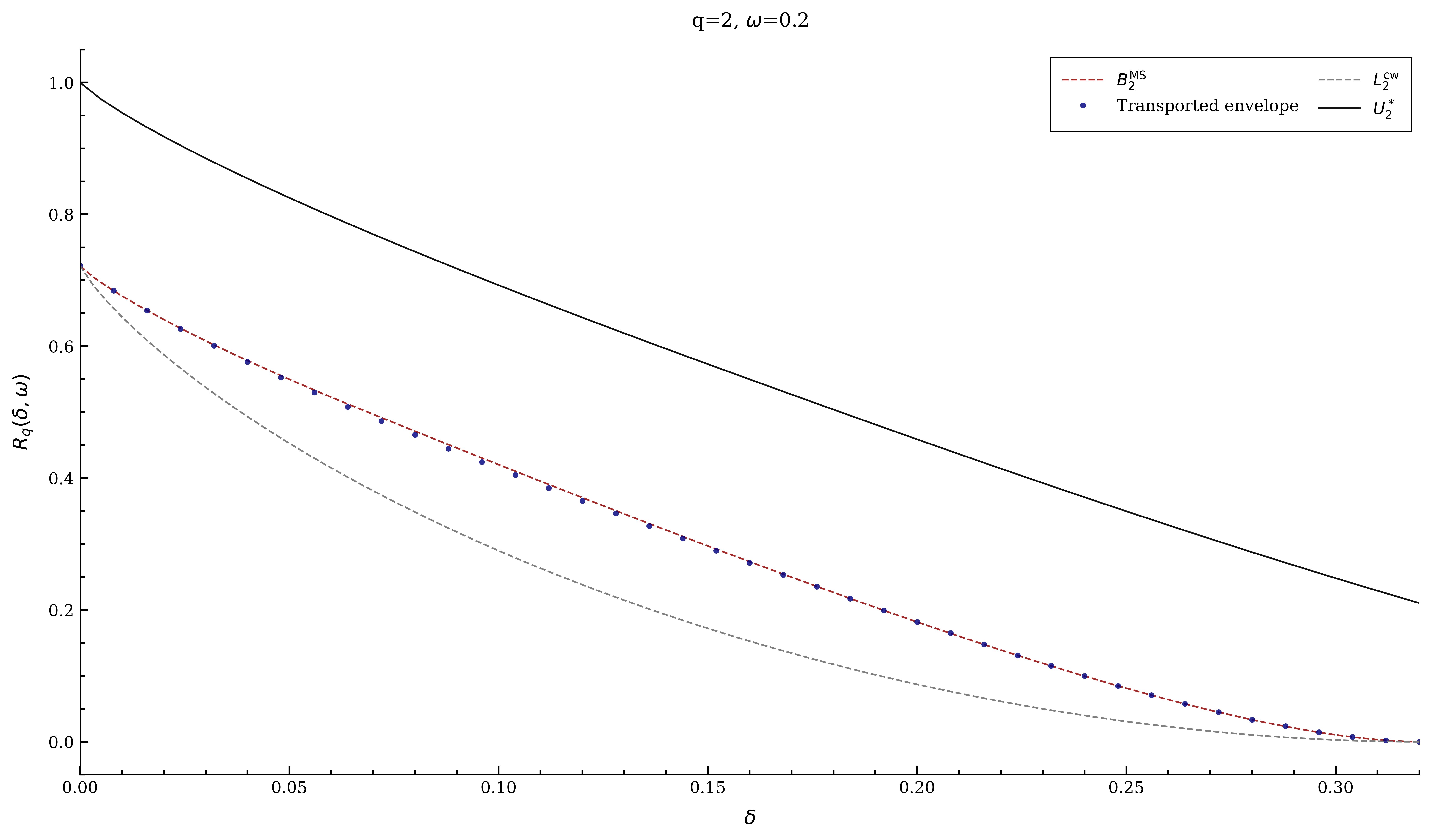
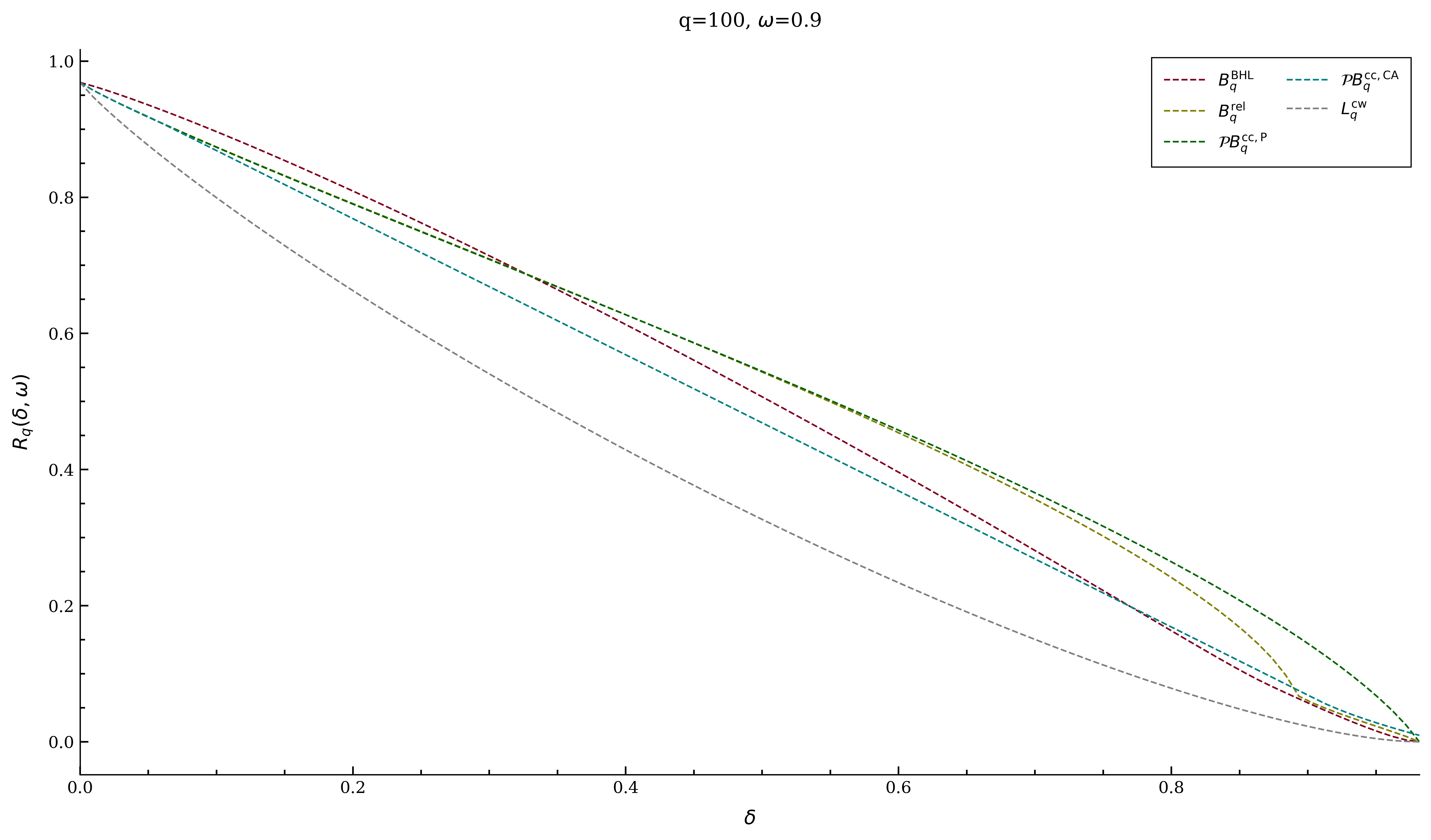
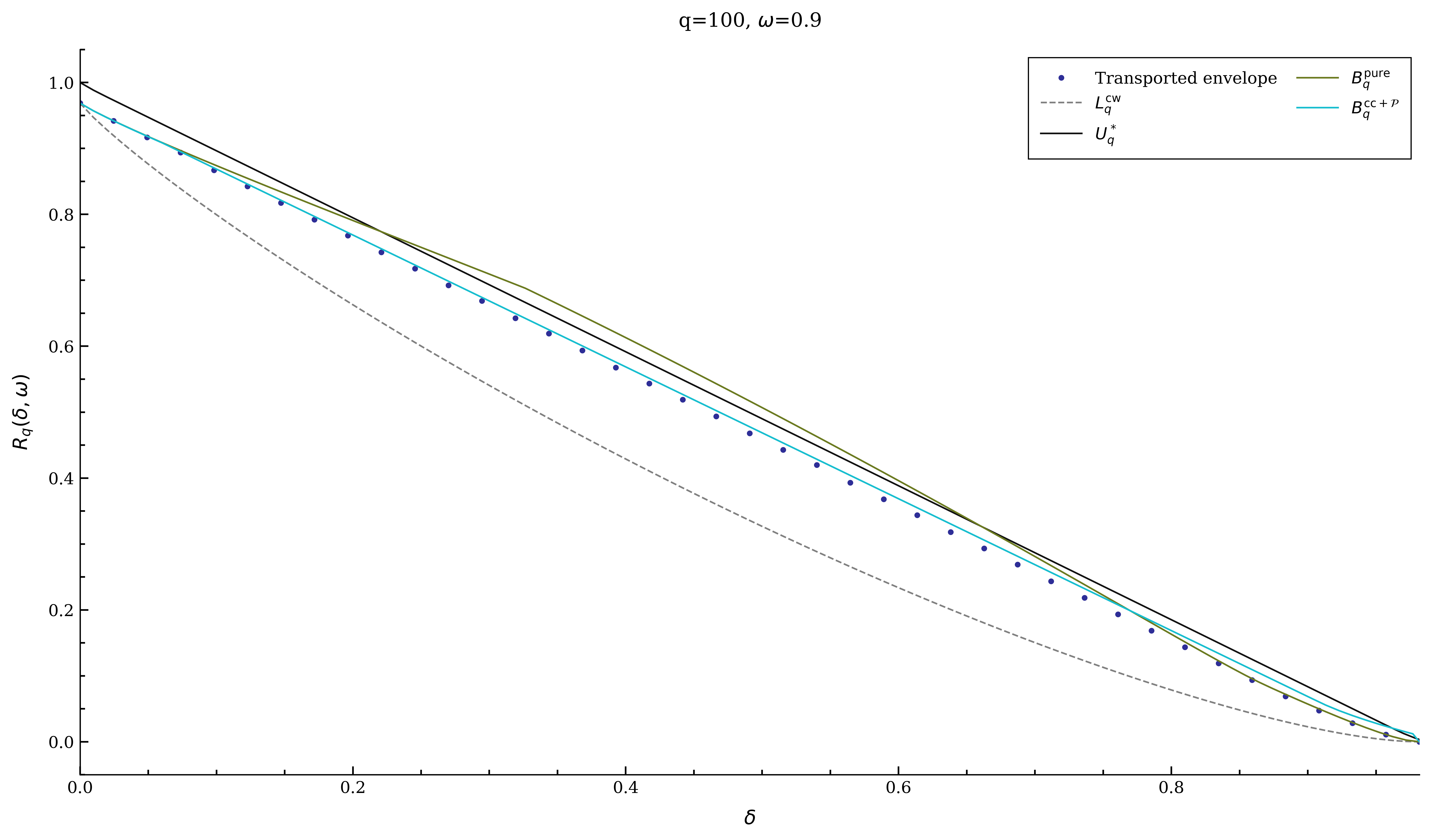
Refer to caption — Figure 1: Binary constant-weight comparison for $q=2$ and $\omega=0.2$ : the moving-subspace Johnson-layer input (red dashed), its permutation transport (blue dots), the unrestricted envelope (black solid), and Varshamov–Gilbert lower bound (gray dashed).

Permutation transport produces an improvement already in the binary example and this improvement becomes more visible for large $q$ .

7.2 Non-symmetric composition targets

It is natural to ask whether Theorem 2.1 and Theorem 2.2 give the same asymptotic results. By Proposition 3.7 we know that this is the case when both source and target vectors are symmetric. However, in the example below the optimal upper bound which can be obtained via Theorem 2.2 using the permutation-transport and symbol-merging construction of Corollary 6.2 cannot be obtained by Theorem 2.1. This example uses a symmetric source and an asymmetric target.

Take $\omega=0.99$ , $\delta=0.17$ . The optimal transport $(0.01,0.495,0.495)\longrightarrow(0.01,t,0.99-t)$ is the two-permutation plan (51). Its information cost is $0.99\log_{3}2\,[1-h_{2}(t/0.99)]$ . Merging the rare symbol gives a binary code of relative weight $t$ and relative distance at least $0.15=\delta-2(1-\omega)$ . Formula (50) gives

R_{3}(0.17,0.99)\leq\log_{3}2\inf_{0\leq t\leq 0.495}\left\{0.99\left(1-h_{2}\left(\frac{t}{0.99}\right)\right)+B_{2}^{\mathrm{MS-CW}}(0.15,t)\right\}.

The numerical value obtained at $t=0.11576$ is approximately 0.35623.

Transported Ben-Haim–Litsyn bound $\mathcal{P}B_{3}^{\mathrm{BHL}}(0.17;p_{0.99})$ gives 0.36346, while application of Lemma 6.1 to the constant-weight bound $(\mathcal{P}B_{2}^{\mathrm{MS-CW}})(0.15;p_{0.495})$ gives 0.36134.

References

[1] M. Aaltonen (1990) A new upper bound on nonbinary block codes. Discrete Mathematics 83, pp. 139–160. Cited by: §5.6.
[2] R. Ahlswede and L. H. Khachatrian (1997) The complete intersection theorem for systems of finite sets. European Journal of Combinatorics 18 (2), pp. 125–136. Cited by: §5.3.
[3] R. Ahlswede and L. H. Khachatrian (1998) The diametric theorem in Hamming spaces—optimal anticodes. Advances in Applied Mathematics 20, pp. 429–449. Cited by: §5.3, §5.6.
[4] O. Alrabiah and V. Guruswami (2026) Binary code rate bounds via classical–quantum channels. arXiv preprint arXiv:2608.09347. Cited by: §5.6, §5.6.
[5] C. Bachoc, V. Chandar, G. Cohen, P. Solé, and A. Tchamkerten (2011) On bounded weight codes. IEEE Transactions on Information Theory 57, pp. 6780–6787. External Links: Document, Link Cited by: §1, §4.1.
[6] A. Barg and G. Zémor (2005) Multilevel expander codes. In Proceedings. International Symposium on Information Theory, 2005. ISIT 2005., pp. 1315–1319. Cited by: §5.9.
[7] A. Barg (2026) Comments on the recent improvements of the MRRW bounds. arXiv preprint arXiv:2609.01860. Cited by: §5.7, §5.7, §5.7, §5.7.
[8] P. Beelen (2022) A survey on recursive towers and Ihara’s constant. arXiv preprint arXiv:2203.03310. Cited by: §5.9.
[9] Y. Ben-Haim and S. Litsyn (2007) A new upper bound on the rate of non-binary codes. Advances in Mathematics of Communications 1, pp. 83–92. Cited by: §5.4, §5.6.
[10] T. Berger (1971) Rate distortion theory: a mathematical basis for data compression. Prentice–Hall, Englewood Cliffs, NJ. Cited by: Relation to Erokhin–Pinkston reverse water filling..
[11] R. E. Blahut (1977) Composition bounds for channel block codes. IEEE Transactions on Information Theory 23 (6), pp. 656–674. Cited by: §3.2, §3.2.
[12] È. L. Blokh and V. V. Zyablov (1974) Coding of generalized concatenated codes. Problemy Peredachi Informatsii 10 (3), pp. 45–50. Cited by: §5.9.
[13] F. Cicalese, L. Gargano, and U. Vaccaro (2013) Information theoretic measures of distances and their econometric applications. In 2013 IEEE International Symposium on Information Theory, pp. 409–413. Cited by: §3.3.
[14] F. Cicalese and U. Vaccaro (2002) Supermodularity and subadditivity properties of the entropy on the majorization lattice. IEEE Transactions on Information Theory 48 (4), pp. 933–938. External Links: Document Cited by: §3.3.
[15] G. Cohen, P. Solé, and A. Tchamkerten (2010) Heavy weight codes. In International Symposium on Information Theory, pp. 1120–1124. External Links: Link Cited by: §1.
[16] T. M. Cover and J. A. Thomas (2006) Elements of information theory. 2 edition, Wiley-Interscience, Hoboken, NJ. Cited by: §3.1, §3.1, §3.2, §3.4.
[17] I. Csiszár and J. Körner (2011) Information theory: coding theorems for discrete memoryless systems. 2 edition, Cambridge University Press, Cambridge. Cited by: §3.1.
[18] I. Csiszár (1998) The method of types. IEEE Transactions on Information Theory 44 (6), pp. 2505–2523. External Links: Document Cited by: §3.2.
[19] M. Dalai (2015) Elias bound for general distances and stable sets in edge-weighted graphs. IEEE Transactions on Information Theory 61 (5), pp. 2335–2350. Cited by: §3.2.
[20] P. Delsarte (1973) An algebraic approach to the association schemes of coding theory. Philips Research Reports Supplements 10, pp. 1–97. Cited by: §5.5.
[21] N. D. Elkies (2001) Excellent codes from modular curves. In Proceedings of the thirty-third annual ACM symposium on Theory of computing, pp. 200–208. Cited by: §5.9.
[22] N. D. Elkies (2003) Still better nonlinear codes from modular curves. arXiv preprint math/0308046. Cited by: §5.9.
[23] V. Erokhin (1958) $\varepsilon$ -Entropy of a discrete random variable. Theory of Probability and Its Applications 3, pp. 97–100. Cited by: Relation to Erokhin–Pinkston reverse water filling..
[24] T. Etzion (2021) Non-binary diameter perfect constant-weight codes. IEEE Transactions on Information Theory 68 (2), pp. 891–904. Cited by: §5.3.
[25] W. Gay, F. Granha Jeronimo, and L. Liu (2026) The honeycomb framework for code bounds. arXiv preprint arXiv:2608.20287. Cited by: §5.7.
[26] D. C. Gijswijt, A. Schrijver, and H. Tanaka (2006) New upper bounds for nonbinary codes based on the Terwilliger algebra and semidefinite programming. Journal of Combinatorial Theory, Series A 113, pp. 1719–1731. Cited by: §5.5.
[27] E. N. Gilbert (1952) A comparison of signalling alphabets. Bell System Technical Journal 31, pp. 504–522. Cited by: §5.9.
[28] C. Godsil and K. Meagher (2016) Erdős–ko–rado theorems: algebraic approaches. Cambridge University Press, Cambridge. Cited by: §5.3.
[29] W. C. Huffman, J. Kim, and P. Solé (2021) Concise encyclopedia of coding theory. CRC Press. Cited by: §1.
[30] Y. Ihara (1981) Some remarks on the number of rational points of algebraic curves over finite fields. Journal of the Faculty of Science, University of Tokyo 28 (3), pp. 721–724. Cited by: §5.9.
[31] S. M. Johnson (1962) A new upper bound for error-correcting codes. IRE Transactions on Information Theory 8, pp. 203–207. Cited by: §5.1.
[32] K. Kaipa (2018) An improvement of the asymptotic Elias bound for non-binary codes. IEEE Transactions on Information Theory 64, pp. 5170–5178. Cited by: §5.3, §5.6, §5.6.
[33] T. Laihonen and S. Litsyn (1998) On upper bounds for minimum distance and covering radius of non-binary codes. Designs, Codes and Cryptography 14, pp. 71–80. Cited by: §5.6, §5.6.
[34] V. I. Levenshtein (1971) Upper-bound estimates for fixed-weight codes. Problems of Information Transmission 7, pp. 281–287. External Links: Link Cited by: §1, §2.1, §5.1.
[35] X. Liang (2024) The $q$ -ary Gilbert–Varshamov bound can be improved for all but finitely many positive integers $q$ . arXiv preprint arXiv:2403.08727. Cited by: §5.9.
[36] S. Liu, T. Wu, and C. Xing (2023) Nonlinear codes exceeding the Gilbert–Varshamov and Tsfasman–Vlăduţ–Zink bounds. In Proceedings of the 2023 Annual ACM–SIAM Symposium on Discrete Algorithms (SODA), pp. 4104–4114. External Links: Document, Link Cited by: §5.9.
[37] F. J. MacWilliams and N. J. A. Sloane (1977) The theory of error-correcting codes. Vol. 16, Elsevier. Cited by: §1.
[38] A. W. Marshall, I. Olkin, and B. C. Arnold (2011) Inequalities: theory of majorization and its applications. 2 edition, Springer. External Links: Document, Link Cited by: §3.3.
[39] H. Niederreiter and F. Özbudak (2004) Constructive asymptotic codes with an improvement on the Tsfasman–Vlăduţ–Zink and Xing bounds. In Coding, Cryptography and Combinatorics, Progress in Computer Science and Applied Logic, Vol. 23, pp. 259–275. Cited by: §5.9.
[40] H. Niederreiter and F. Özbudak (2006) Improved asymptotic bounds for codes using distinguished divisors of global function fields. Note: arXiv:math/0611260 External Links: math/0611260, Link Cited by: §5.9.
[41] OpenAI (2026) Ten advances in mathematics and theoretical computer science. Note: Chapter 2, “Improved Bounds for Binary and Spherical Codes,” updated 6 August 2026 Cited by: §1, §5.7.
[42] J. T. Pinkston III (1967) Encoding independent sample information sources. Technical report Technical Report 462, Research Laboratory of Electronics, Massachusetts Institute of Technology. Cited by: Relation to Erokhin–Pinkston reverse water filling..
[43] V. Pless, R. A. Brualdi, and W. C. Huffman (1998) Handbook of coding theory. Elsevier Science Inc.. Cited by: §1.
[44] S. C. Polak (2019) New methods in coding theory. Ph.D. Thesis, University of Amsterdam. Cited by: §5.5.
[45] A. Salmon (2026) The half-rate linear programming bound for binary codes is $1/2-1/\pi$ . arXiv preprint arXiv:2609.03736. Cited by: §5.7.
[46] A. Samorodnitsky (2001) On the optimum of Delsarte’s linear program. Journal of Combinatorial Theory, Series A 96 (2), pp. 261–287. External Links: Document, Link Cited by: §1, §4.1, §4.2.
[47] A. Schrijver (2005) New code upper bounds from the Terwilliger algebra and semidefinite programming. IEEE Transactions on Information Theory 51, pp. 2859–2866. Cited by: §5.5.
[48] C. E. Shannon (1948) A mathematical theory of communication. Bell System Technical Journal 27, pp. 379–423, 623–656. Cited by: §3.1.
[49] A. Somekh-Baruch, J. Scarlett, and A. G. i Fabregas (2019) Generalized random Gilbert–Varshamov codes. IEEE Transactions on Information Theory 65 (6), pp. 3452–3469. Cited by: §5.9.
[50] H. Tarnanen, M. Aaltonen, and J. Goethals (1985) On the nonbinary Johnson scheme. European Journal of Combinatorics 6, pp. 279–285. Cited by: §5.5.
[51] M. A. Tsfasman, S. G. Vlăduţ, and T. Zink (1982) Modular curves, Shimura curves, and Goppa codes, better than Varshamov–Gilbert bound. Mathematische Nachrichten 109, pp. 21–28. Cited by: §5.9.
[52] M. A. Tsfasman and S. Vlăduţ (2008) Algebraic-geometric codes. Non-Binary Error Control Coding for Wireless Communication and Data Storage. Cited by: §1.
[53] R. R. Varshamov (1957) Estimate of the number of signals in error correcting codes. Doklady Akademii Nauk SSSR 117, pp. 739–741. Note: In Russian Cited by: §5.9.
[54] C. Xing (2011) Asymptotically good nonlinear codes from algebraic curves. IEEE transactions on information theory 57 (9), pp. 5991–5995. Cited by: §5.9.
[55] V. V. Zyablov (1971) An estimate of the complexity of constructing binary linear cascade codes. Problemy Peredachi Informatsii 7 (1), pp. 5–13. Cited by: §5.9.

Appendix A. Connection with rate–distortion

We now record the rate–distortion interpretation of the profiles obtained in Section 3.4.

Proposition 7.1 (Exact reduction to Hamming information).

Let $X\sim p$ , where $p$ is an arbitrary probability vector on $\mathcal{A}$ . For every $\theta\in[0,1]$ ,

K_{q}(p,p_{\theta})=\min_{P_{Z\mid X}:\,\Pr\{X\neq Z\}=\theta}I_{q}(X;Z),

(56)

where $Z$ takes values in $\mathcal{A}$ .

Proof.

For any feasible permutation transport, put $Z=\Pi^{-1}(0)$ . Then $\Pi(X)=0$ if and only if $X=Z$ , so $\Pr\{X\neq Z\}=\theta$ . Since $Z$ is a function of $\Pi$ , data processing inequality (9) gives $I_{q}(X;Z)\leq I_{q}(X;\Pi)$ .

Conversely, given a joint distribution of $(X,Z)$ with exact error probability $\theta$ , choose $\Pi$ , conditionally on $Z=z$ , uniformly among the $(q-1)!$ permutations satisfying $\Pi(z)=0$ , independently of $X$ given $Z$ . The output is zero when $X=Z$ and is uniform on $\mathcal{A}\setminus\{0\}$ otherwise. Hence $\Pi(X)\sim p_{\theta}$ . Moreover, $Z$ is determined by $\Pi$ and $X\to Z\to\Pi$ is a Markov chain, so $I_{q}(X;\Pi)=I_{q}(X;Z)$ . ∎

Relation to Erokhin–Pinkston reverse water filling.

For a discrete source $X\sim p$ and Hamming distortion, the classical rate–distortion function is

\mathsf{R}_{p}(D):=\min_{P_{Z\mid X}:\,\Pr\{X\neq Z\}\leq D}I_{q}(X;Z)=\min_{0\leq\theta\leq D}K_{q}(p,p_{\theta}),\qquad 0\leq D\leq 1,

where $Z$ takes values in the same alphabet $\mathcal{A}$ , and the second equality follows from Proposition 7.1. The explicit solution due to Erokhin and Pinkston is commonly described as reverse water filling [23, 42, 10]: as the allowed distortion increases, the least probable symbols successively leave the support of an optimal reproduction distribution. The function $\mathsf{R}_{p}(D)$ becomes zero at $D=1-\max_{x}p_{x}$ and remains zero thereafter.

In contrast, the transport cost $K_{q}(p,p_{\theta})$ corresponds to the exact error probability $\Pr\{X\neq Z\}=\theta$ , as established in (56). It need not be nonincreasing in $\theta$ and may become positive again after its zero-information interval. Thus the classical rate–distortion function is obtained by minimizing the exact-distortion profile over all errors not exceeding $D$ , rather than by evaluating that profile at $\theta=D$ . The join formula in Theorem 3.2 provides a single geometric description of the entire exact-distortion profile.