On Generalized Naive Bayes with Continuous Features

Ábrahám Papp Address: Department of Analysis and Operations Research, Institute of Mathematics, Budapest University of Technology and Economics Botond Szilágyi Address: Department of Chemical and Environmental Process Engineering, Faculty of Chemical Technology and Biotechnology, Budapest University of Technology and Economics Edith Alice Kovács Address: Department of Analysis and Operations Research, Institute of Mathematics, Budapest University of Technology and Economics

Abstract

The Generalized Naive Bayes (GNB) model was introduced for discrete and categorical random variables as an extension of classic Naive Bayes. We now accommodate the GNB framework to continuous explanatory variables. A central result of the paper is that structure learning of the GNB depends only on the pair copulas of the bi-variate marginals. We proved that the GNB structure can be assigned to the basis of a matroid, therefore we give greedy algorithms for finding the optimal GNB structure on the training data, in sense of minimizing Kullback-Leibler divergence. Three cases are considered: joint Gaussian distribution, then a more flexible model where we suppose the dependence structure to be described by a Gaussian copula with arbitrary marginals, and an even more flexible case where the joint continuous probability distribution is arbitrary, i.e. copula and marginal distributions are arbitrary. A method for model reduction, based on the newly introduced concept of GNB forest is given. We close the paper by comparing the newly introduced GNB classification results to other classical "glass-box" algorithms on real datasets.

Keywords:

Naive Bayes, Gaussian GNB, General GNB, Gaussian copula GNB , classification, structure learning

MSC

62C12 , 62C10 , 62-07

^†^†highlights: The Generalized Naive Bayes (GNB) structure is extended to the case of continuous explanatory variables. It is proven that finding the GNB structure, depends only on the joint copula of the feature pairs. We discuss the combinatorial properties of the GNB structures. Greedy algorithms for GNB structure discovering under three dependence scenarios are given. Classification algorithms are given using the whole and reduced GNB structure.

1 Introduction

Naive Bayes classifier is one of the most popular machine learning algorithms due to its simplicity, efficiency and easy interpretation, which is appealing to experts in various domains. Therefore, it is considered to be one of the top 10 data mining algorithms [1], [2]. However, most real-world domains involve continuous variables. A common practice to deal with continuous variables is to discretize them, with a subsequent loss of information. In this paper we are especially interested in cases when the explanatory variables are continuous.

To illustrate the ubiquitous interest in this algorithm we provide a glimpse of some recent applications of it. Gaussian Naive Bayes classification is applied for detector pulse discrimination, see [3]. In [4] a new class-specific feature selection is proposed, instead of using the same features for all classes. For probability estimation authors use kernel density estimation. A new efficient classification weighted Naive Bayes classifier was introduced in [5]. The probabilities were weighted based on a mean of three weights mutual information, chi-square (independence test) and Gini impurity calculated on discretized data. We consider very important to mention here the study [6] where an approach for building optimized machine learning models for the classification of opinions on social media posts is proposed. Their experiments shown that although RNN architectures are widely recognized for their ability to handle sequential data, classical algorithms such as Naive Bayes and SVM still offer comparable performance, especially when preprocessing techniques were used. They showed that Naive Bayes outperformed RNN on most datasets.

An emerging problem today is the management of decentralized data sources while preserving data privacy. The paper [7] proposes a new federated approach for Naive Bayes (NB) classification, assuming discrete variables. Their approach federates a discriminative variant of NB, sharing meaningless parameters instead of conditional probability tables. Therefore, this process is more reliable against possible attacks.

The NB algorithm is based on the assumption that the explanatory variables are conditionally independent given the class variable (target variable). This is not generally true for real-life problems. Many papers are concerned with the improvement of this remarkable algorithm. These improvements follow mainly two directions. Some research show that selecting some attributes beforehand might result in better classification accuracy and better generalization. Another improvement might be achieved by relaxing the conditional independence assumption. Essential results in this direction, using continuous predictors without discretizations, are introduced in the following papers. In [8] a former method, called Tree Augmented Naive Bayes (TAN) [9] which was defined for discrete attributes, was extended to continuous attributes having Gaussian or mixture or Gaussian distributions. Furthermore, they proposed a hybrid model that can simultaneously accommodate both continuous and discrete variables. In [10], the application of conditional Gaussian distributions was further investigated and adapted to this framework. The study also introduced the $k$ -Dependence Bayesian classifier, originally proposed for the discrete setting in [11]. In Sahami’s paper [11], the $k$ -dependence classifier includes the structure of a Naive Bayes classifier and allows each feature to have at most $k$ parent features. In [10] the authors improved the former method and called it filter $k$ -dependence Bayes classifier. In [12], the authors examined the classification framework from the perspective of Bayesian networks, which represent conditional independence relationships among random variables using directed acyclic graphs. They proposed several flexible classifiers based on kernel density estimation, including the Flexible Naive Bayes, Flexible Tree-Augmented Naive Bayes, and Flexible $k$ -Dependence Bayesian classifiers (FKDB). In the FKDB model, each predictor variable is allowed to have at most $k$ parent predictors in addition to the class variable, thereby providing greater modeling flexibility while controlling structural complexity. Conditional mutual information between the features with respect to the classifier is considered in their greedy algorithms. A novel selective Naive Bayes algorithm was introduced in [13], where after ordering the features based on the mutual information between the features and target variable, each new model is obtained from the previous one by adding one feature greedily. The "nest" model is chosen based on its predictability power. In [14] authors gave a new version of Naive Bayes classifier dealing with datasets with correlated patterns. The method involves reducing variables through clustering, based on their dependencies. The goal was to select a combination of features that are as independent as possible.

There are also some recent papers dealing with $k$ -dependence classifiers. In [15] for each node up to $k$ parents are added in greedy way taking into account the conditional log-likelihood. Another paper concerning with the introduction of higher order dependencies into a Bayesian network classifier is [16]. Their idea is to start from a TAN structure and to add directed edges based on conditional entropy. Although increasing the value of $k$ may raise the risk of overfitting, fixing $k$ may constrain the model flexibility. To address these issues in [17], the authors propose $K$ -free dependence Bayesian classifiers, which can learn an adaptive number of parent nodes for each attribute. To search its optimal structure, they sequentially evaluate the candidate submodels either by minimizing the mean squared error or maximizing the classification accuracy.

A very interesting new paper [18] improves the Gaussian Naive Bayes classifier on imbalanced datasets through coordinate-based minority feature mining, using coordinate transformation based on local relative density changes. In [19] a relaxed Naive Bayesian classifier was introduced based on the maximum dependent attribute groups, is proposed to alleviate the conditional independence assumption and then to obtain better prediction performance than traditional Naive Bayes and its most of variants.

Ensemble learning can also lead to performance improvement. In [20] random Bayes forest is proposed by introduction of randomness (via a probability distribution on the mutual information) in root selection, children selection and parent selection. The classification is delivered by voting.

A comparison of the three main methods for handling continuous variables: the normal method, the kernel method, and discretization is given in [21]. They showed that no single method is universally better than the other. The authors present three model-selection methods based on cross-validation that can significantly improve overall performance of Naive Bayes classifiers, outperforming any of the three popular methods on their own.

The present paper aims to relax the conditional independence assumption by introducing a structure that allows dependencies among the explanatory attributes. We create the theoretical background for the case of continuous attributes, then we extend the graphical structure allowing more complex dependencies. We discuss on the optimality of the greedy algorithms introduced. We also compare classification results to other "glass-box" methods like support vector machine (SVM) and logistic regression (LR). We mention here the paper [22] of Ng et.al. which compares Naive Bayes algorithm with logistic regression. They claimed that there exist two distinct regimes of performance between the generative and discriminative classifiers with regard to the training-set size. Another paper [23] suggests through simulation that the existence of the two distinct regimes may not be so reliable. In addition, for real world datasets, so far there is no theoretically correct, general criterion for choosing between the discriminative and the generative approaches for classification. The choice depends on the confidence we have in the correctness of the specification of either $p(y|\mathbf{x})$ or $p(\mathbf{x},y)$ .

The remainder of this paper is organized as follows. In Section 2, key concepts and main results from probability theory, information theory and graph theory needed are introduced. Section 3 introduces the weights assigned to the approximation under different assumptions on the joint distribution of the explanatory variables. This section contains the proof that the structure of GNB depends only on the copula of the features, which gives an absolutely new perspective to this field.

In Section 4, we discuss the combinatorial background of the GNB structures and give greedy algorithms which guarantee to find the optimal structure on the training data in the sense of minimizing Kullback-Leibler divergence under different dependence assumptions. Moreover we introduce the $k$ -GNB model which allows even more complex dependence structure between the continuous explanatory variables. In Section 5 two classification procedure are given. The first one uses all explanatory feature. We give a reduction method based on $f1$ score which uses a subset of features and based on this we introduce the second classification procedure. In section 6 numerical results and comparisons with other glass-box algorithms are presented. We close the paper with conclusions and future work 7.

2 Preliminaries

Naive Bayes is a fast and effective classification method with a clear theoretical foundation, although its primary drawback is the conditional independence assumption.

In this paper, we will use the extension of the Naive Bayes structure to the Generalized Naive Bayes (GNB) structure by allowing dependencies between the explanatory variables. However, we want to exploit beside their dependencies the conditional independencies between them also. The GNB structure was introduced as a special case of the discrete cherry trees in a recent paper [24]. Now, we approach the case when the explanatory variables are continuous and are not conditionally independent given the class variable. Previous papers concerned with allowing dependence between explanatory variables typically do only discuss on conditional independence when they relate the structure to Bayes networks, which are described by directed acyclic graphs [10], [12], [8],[15].

The GNB model with continuous explanatory variables is a special probabilistic mixed graphical model that includes both a discrete target variable and continuous explanatory variables. Therefore the concepts we use are coming from different fields like probability theory, graph theory, information theory, and optimization.

However, in general the structure learning of the probabilistic graphical models is challenging, due to the combinatorial search required across all potential structures is NP complete [25]. In our approach the dimension of the marginal distributions involved remains bounded, this way, the search space for finding the best-fitting structure to the real distribution described by the sample data, is also massively reduced.

The following subsections summarize key concepts and preliminary results essential for the new findings presented in the paper.

2.1 The GNB structures

The GNB graph structure was introduced in [24] as a special case of the cherry-tree structure introduced in [26] [27], see A for the general definition of the cherry tree. Since we use the same graph structure as in [24] we define it directly.

Definition 1.

A Generalized Naive Bayes graph-structure on $V=D\cup\left\{0\right\}=\\$ $=\left\{0,1,\ldots,d\right\}$ (vertex 0 is assigned to $Y$ ), is constructed as follows:

•

Step 1. The smallest GNB structure on three vertices is given by the interconnected triplet $\left(0,i_{1},i_{2}\right)$ , where $i_{1},i_{2},\in D$ .
•

Step k. Let us suppose that the vertices $i_{1},i_{2},\ldots,i_{k}\in D$ are already in the GNB structure. We add a new vertex $i_{k+1}\in D$ to the existing GNB structure by connecting it to vertex $0$ and an already connected vertex $i_{m}\in\left\{i_{1},i_{2},\ldots,i_{k}\right\}$ . The vertex $i_{m}$ is called the mother of vertex $i_{k+1},k>0$ , denoted by $\mu(i_{k+1})$ .

Refer to caption — Figure 1: Construction of a GNB graph on 6 vertices. $0$ corresponds to the target variable while the other vertices to the explanatory variables

We call GNB-junction tree the structure assigned to the GNB graph structure the following way:

1.

The set of vertices in each $3$ - element maximum clique (fully connected subgraph) is called a cluster containing its $3$ vertices (a node in the junction tree graph).
2.

Two $3$ -element clusters are connected if the following two conditions are fulfilled: (a) the clusters share $2$ elements; (b) if a set of $2$ elements is contained by $m$ clusters, these clusters will be connected tree-like by $m-1$ edges, see second row of Figure 2.
3.

The $2$ -element set given by the intersection of two connected clusters is called a separator. The number of clusters containing it is called the multiplicity of the separator.

For an illustration of a GNB-structure, corresponding to a GNB graph, see first row in Figure 2. The junction trees associated with a GNB graph structure in second row of Figure 2 do not have a unique graph representation, but all can be represented in a compact form Figure 2, third row.

Let $\mathbf{X}=\left(X_{1},\ldots,X_{d}\right)^{T}$ a random vector of the explanatory variables and $D$ $=\{1,...,d\}$ the set of indices. The GNB-junction tree over $V=D\cup 0$ given by the set of clusters $\mathcal{C}$ , the set of separators $\mathcal{S}$ together with the separators multiplicity set $\mathcal{M}$ denoted by $(V,\mathcal{C},\mathcal{S},\mathcal{M})$ . For convenience we will use the following notations: the probability distribution of a random vector with its components $(X_{i_{1}},\ldots,X_{i_{k}})$ is shortened as follows: $p(\mathbf{X}_{i_{1},\ldots,i_{k}})$ and $p(\mathbf{X}_{A})$ where $A=\{i_{1},\ldots,i_{k}\}\subset V$ .

The probability distribution corresponding to a GNB-junction tree $(V,\mathcal{C},\mathcal{S},\mathcal{M})$ is given by the following formula:

p_{GNB}(\mathbf{x})=\frac{\prod\limits_{C\in\mathcal{C}}p\left(\mathbf{x}_{C}\right)}{\prod\limits_{S\in\mathcal{S}}p\left(\mathbf{x}_{S}\right)^{v_{S}-1}}=\frac{\prod\limits_{(l,m,0)\in\mathcal{C}}p\left(\mathbf{x}_{l,m,0}\right)}{\prod\limits_{(s,0)\in\mathcal{S}}p\left(\mathbf{x}_{s,0}\right)^{v_{S}-1}}

(1)

where $v_{S}$ is the number of clusters that are connected through the separator $S=(s,0)$ (multiplicity of $S$ ); the formula stands for all realizations of $\mathbf{X}$ .

One can note that, regardless of which graphical representation of a junction tree we use (see, for example, Figure 2), the probability distribution associated has the same formula. In our example this is:

P_{GNB}\left(\mathbf{x}\right)=\frac{p(\mathbf{x}_{0,1,2})p(\mathbf{x}_{0,2,3})p(\mathbf{x}_{0,1,4})p(\mathbf{x}_{0,1,5})}{(p\left(\mathbf{x}_{0,1}\right))^{2}p\left(\mathbf{x}_{0,3}\right)}.

2.2 Results related to copula theory

In 1959 Abe Sklar introduced copula functions [28], which are capable of modeling the dependence between variables separate from the one-dimensional marginals.

Let $\boldsymbol{X}=(X_{1},\dots,X_{d})\in\mathbb{R}^{d}$ be an $d$ -dimensional continuous random vector, with $p$ joint p.d.f. and $F$ joint c.d.f., meaning that

F(x_{1},\dots,x_{d})=\mathbb{P}(X_{1}\leq x_{1},\dots,X_{d}\leq x_{d}).

Definition 2.

A function $C:[0,1]^{d}\to[0,1]$ is an $d$ -dimensional copula function, if it satisfies the following properties:

•

$C(u_{1},\dots,u_{d})$ is strictly increasing in all $u_{i}$ components.
•

$C(u_{1},\dots,u_{i-1},0,u_{i+1},\dots,u_{d})=0$ for all $u_{k}\in[0,1]$ , $k\neq i$ , $i\in\{1,\dots,d\}$ .
•

$C(1,\dots,1,u_{i},1,\dots,1)=u_{i}$ for all $u_{i}\in[0,1]$ , $i\in\{1,\dots,d\}$ .
•

$C$ is $d$ -increasing, meaning that for all $(u_{1,1},\dots,u_{1,d})$ and $(u_{2,1},\dots,u_{2,d})$ in $[0,1]^{n}$ , if for all $i$ , $u_{1,i}<u_{2,i}$ , then

$\sum_{i_{1}=1}^{2}\cdots\sum_{i_{d}=1}^{2}(-1)^{\sum_{j=1}^{d}i_{j}}C(u_{i_{1},1},\dots,u_{i_{d},d})\geq 0$

In the theory of copulas, Sklar’s theorem (1959) [28] can be regarded as a central theorem:

Theorem 3.

Any multivariate c.d.f. $F$ can be written in the following way:

F(x_{1},\dots,x_{n})=C(F_{1}(x_{1}),\dots,F_{n}(x_{n}))

Moreover, if the one-dimensional marginals $F_{1},\dots,F_{d}$ are continuous, then $C$ in unique.

The following formula connects the original density function with the copula density:

p(x_{1},\dots,x_{d})=c(F_{1}(x_{1}),\dots,F_{n}(x_{d}))\cdot p_{1}(x_{1})\cdot\dots\cdot p_{d}(x_{d})

(2)

Where $c$ is the joint p.d.f. of $\boldsymbol{U}=(U_{1},\dots,U_{n})$ or the mixed partial derivative of $C$ .

An interesting overview is given in [29]

2.3 Information theoretical concepts

Since the best-fitting GNB probability distribution is achieved by minimizing the Kullback-Leibler divergence we recall the necessary information theoretical concepts. For more details, see the fundamental book [30].

We will use an equivalent formulation of conditional entropy that quantifies the amount of information needed to describe the outcome of a random variable $Y$ given a random variable $X$ : $H(Y|X)=H(X,Y)-H(X)$ .

We will use the following formula for the information content of a bi-variate mixed random variable consisting of $X$ continuous and $Y$ discrete random variables:

I(\mathbf{X})=H(X)+H(Y)-H(X,Y)

(3)

where: $H(Y)$ stands for the entropy of a discrete random variable $Y$ : $H(Y)=-\sum_{y\in\mathcal{Y}}p(y)\log p(y)$ ; $H(X,Y)$ is the joint entropy of a continuous variable $X$ and a discrete variable $Y$ : $H(X,Y)=-\sum_{y\in\mathcal{Y}}\int_{\mathcal{X}}p(x,y)\log p(x,y)\,dx$ , and $\chi$ is the domain of the random variable $X$

When a $p(\mathbf{x})$ probability density is approximated by $p_{app}(\mathbf{x})$ the quantification of the information loss is given by the Kullback-Leibler divergence (KL-divergence) [31]:

\mathbf{KL}(p(\mathbf{x}),p_{app}(\mathbf{x}))=\int_{\chi}p\left(\mathbf{x}\right)\log_{2}\frac{p\left(\mathbf{x}\right)}{p_{app}(\mathbf{x})}d\mathbf{x}.

(4)

KL divergence is a positive number unless $P_{app}\equiv P$ , when $\mathrm{KL}=0$ . The smaller the value of the KL-divergence is the better the approximation is.

The mutual information can be seen as a special type of KL divergence between a given $p(X_{i_{1}},X_{i_{2}})$ and an approximation given by independence: $p_{app}=p(X_{i_{1}})p(X_{i_{2}})$ .

The information content of a random vector $\mathbf{X}=(X_{i_{1}},...,X_{i_{k}})$ can be given straightforward as a generalizations of the mutual information:

I(X_{i_{1}},...,X_{i_{k}})=\int_{\mathbf{\chi}}p\left(x_{i_{1}},\dots,x_{i_{k}}\right)\log_{2}\frac{p\left(x_{i_{1}}\mathbf{,}\dots,x_{i_{k}}\right)}{p(x_{i_{1}})\cdot\ldots\cdot p(x_{i_{k}})}d\mathbf{x}.

(5)

or more general by the following formula

I(\mathbf{X})=\sum\limits_{t=i_{1}}^{i_{k}}H(X_{t})-H(\mathbf{X})

(6)

We note that the information content defined above and used in the papers [26] and [27] quantifies the strength of the dependence between the random variables; it was also called by other authors as multiinformation or total correlation.

A fundamental theorem we use in this paper is an adaptation of the general result of the KL divergence between the real probability distribution and an approximation given by a general cherry tree [27]. We are now interested in the case when the approximation is given by a GNB junction tree. The expression of the KL divergence between a real probability distribution and a GNB junction tree probability distribution involves marginals of order two and three corresponding to the separators and clusters, see [24]:

Theorem 4.

The Kullback-Leibler divergence between the real distribution $P(\mathbf{X})$ and the GNB junction tree approximation (1) is:

	$\displaystyle KL(P\left(\mathbf{X}Y\right),P_{GNB}\left(\mathbf{X}Y\right))$	$\displaystyle=\sum\limits_{i=1}^{d}H(X_{i})+H(Y)-H(\mathbf{X,}Y)$
		$\displaystyle-\left(\sum\limits_{C\in\mathcal{C}}I\left(\mathbf{X_{C}}\right)-\sum_{S\in\mathcal{S}}(\nu_{s}-1)I\left(\mathbf{X_{S}}\right)\right),$		(7)

where the clusters $C$ and the separators $S$ contain the index 0 corresponding to the target variable.

Since KL depends on the structure of the GNB only through the amount in the parenthesis, we introduce the following definition.

Definition 5.

We call the weight of the approximation the following sum:

W=\sum\limits_{C\in\mathcal{C}}I(\mathbf{X}_{C})-\sum\limits_{S\in\mathcal{S}}\left(\nu_{s}-1\right)I(\mathbf{X}_{S})

(8)

Since the weight is positive or zero, a larger weight results in a better approximation. Therefore, we conclude that it is worthwhile to find the structure with the largest weight.

In [24] it was proved that the GNB approximation provides an approximation to the training data that is at least as good as that of the NB approximation

In the present paper we deal with continuous features, which do not alter the formula and our objective because all information contents are positive or $0$ . (Differential entropy for example does not preserve this property in the continuous case.) We aim to maximize the weight; a problem which occurs is that information contents depend on a discrete random variable (the classifier) and continuous random variables at the same time. Therefore we have to introduce the information content of a mixed random vector.

The information contents of a mixed random vector

We introduce the following notations which are used throughout the paper: $p(\mathbf{x},y)$ is the joint probability density/mass function of $\mathbf{X}$ and $Y$ , $p_{i}(x_{i})$ denotes the uni-variate marginal probability density function of $X_{i}$ , whereas $p(\mathbf{x})$ denotes the multivariate probability density function of the random vector $\mathbf{X}=(X_{1},...,X_{d})$ , $p(y)$ is the probability distribution of the discrete random variable (classifier) $Y$ . In our present setting $\mathbf{X}$ the random vector containing continuous attributes and the discrete, target random variable $Y$ that takes on values in the set $\mathcal{Y}=\{y_{1},...,y_{m}\}$ .

Theorem 6.

The formula for the information content of a random vector consisting of $d$ continuous explanatory variables $\mathbf{X}=(X_{1},...,X_{d})$ and a discrete variable $Y$ is the following:

I(\mathbf{X},Y)=\sum\limits_{i=1}^{d}H(X_{i})-\sum\limits_{y_{k}\in\mathcal{Y}}p(y_{k})H(\mathbf{X}|y_{k}).

(9)

For the proof see B

3 The weight of a GNB approximation under different assumptions on the joint distribution of the explanatory variables

In the Subsection 2.3, we pointed out that the weight of the approximation of the approximation connects the GNB structure to the goodness of fit. In this chapter we examine three cases. In the first case, we assume that the explanatory variables follow a multivariate Gaussian distribution then we discuss the general case when the joint probability distribution is expressed by the means of copulas, with arbitrary marginal distributions. In the last case we consider Gaussian copula to model the dependence structure, and arbitrary marginals to model the features.

3.1 Features following joint Gaussian distribution

In this subsection, we suppose the target to be a discrete variable and the explanatory variables to have a joint Gaussian distribution with mean vector $\mu_{\mathbf{X}}$ and covariance matrix $\mathbf{K}_{\mathbf{X}}$ . This seems to be quite restrictive, but there are many cases when this works very well. In order to calculate the weight of the approximation, the mixed information content of orders two and three have to be calculated. We also will use that all marginals of a Gaussian distribution are Gaussian.

The weight of the Gauss-GNB structure

First, we derive the formula for the information content of a bi-variate random vector consisting of a continuous Gaussian random variable $X$ and a discrete random variable $Y$ . For convenience, we use the natural logarithm. The uni-variate Gaussian entropy is given by formula: $H(X)=\frac{1}{2}\log(2\pi e\sigma^{2})$ .

The mutual information between a continuous variable $X$ with Gauss distribution and a discrete variable $Y$ is given by the following formula. (The proof is given in C)

\displaystyle I(X,Y)=\frac{1}{2}\left(\log\sigma^{2}_{X}-\sum\limits_{y_{k}\in\mathcal{Y}}p(y_{k})\log\sigma^{2}_{X|y_{k}}\right)

(10)

Now, we deduce a general formula for the information content of a continuous multivariate Gaussian distribution over $\mathbf{X}$ with covariance matrix $\mathbf{K}$ and a discrete random variable $Y$ . We start from formula 9 and use besides the formula of the entropy of a uni-variate Gaussian distribution the entropy of the $d$ dimensional Gaussian distribution:

\displaystyle H(\mathbf{X})

\displaystyle=

\displaystyle\frac{1}{2}\left[\log(2\pi e)^{d}\left|K_{\mathbf{X}}\right|\right]

$\displaystyle I(\mathbf{X},Y)$	$\displaystyle=$	$\displaystyle\sum\limits_{i=1}^{d}H(X_{i})-\sum\limits_{y_{k}\in\mathcal{Y}}p(y_{k})H(\mathbf{X}\|y_{k})=$	(11)
	$\displaystyle=$	$\displaystyle\sum\limits_{i=1}^{d}\frac{1}{2}\log(2\pi e\sigma_{X_{i}}^{2})-\sum\limits_{y_{k}\in\mathcal{Y}}p(y_{k})\left(\frac{1}{2}\log\left(2\pi\right)^{d}+\frac{1}{2}\log\left\|K_{\mathbf{X}\|y_{k}}\right\|+\frac{d}{2}\right)=$
	$\displaystyle=$	$\displaystyle\frac{1}{2}\left[\sum\limits_{i=1}^{d}\left(\log 2\pi+1+\log\sigma_{X_{i}}^{2}\right)-\left(d\log\left(2\pi\right)+d\right)\sum\limits_{y_{k}\in\mathcal{Y}}p(y_{k})\right]-$
		$\displaystyle-\frac{1}{2}\sum\limits_{y_{k}\in\mathcal{Y}}p(y_{k})\log\left\|K_{\mathbf{X}\|y_{k}}\right\|=$
	$\displaystyle=$	$\displaystyle\frac{1}{2}\left[\sum\limits_{i=1}^{d}\log\sigma_{X_{i}}^{2}-\sum\limits_{y_{k}\in\mathcal{Y}}p(y_{k})\log\left\|K_{\mathbf{X}\|y_{k}}\right\|\right]$

As we saw in the preliminaries, KL divergence depends on the GNB structure only through its weight, which depends on the information content of the clusters and the separators in the GNB structure 8.

As a particular case for formula 11 we express $I(X_{l},X_{m},Y)$ as

\displaystyle I(X_{l},X_{m},Y)=\frac{1}{2}\left[\log\sigma_{l}^{2}+\log\sigma_{m}^{2}-\sum\limits_{y_{i}\in\mathcal{Y}}p(y_{i})\log|K_{X_{l}X_{m}|y_{i}}|\right]

(12)

Based on 10 and 12 we will deduce the formula of weight.

Theorem 7.

The weight of a GNB distribution corresponding to the $(V,\mathcal{C},\mathcal{S},\mathcal{M})$ GNB structure with joint Gaussian explanatory variables is:

	$\displaystyle W$	$\displaystyle=$	$\displaystyle\frac{1}{2}\log\prod\limits_{m\in D}\sigma_{m}^{2}-\frac{1}{2}\underset{y_{i}\in\mathcal{Y}}{\sum}p(y_{i})\log\left(\prod\limits_{m\in D}\sigma_{m\|yi}^{2}\right)+$		(13)
		$\displaystyle-$	$\displaystyle\frac{1}{2}\underset{y_{i}\in\mathcal{Y}}{\sum}p(y_{i})\sum\limits_{(l,m,0)\in\mathcal{C}}\log(1-\rho^{2}_{lm\|y_{i}})$		(13)

where $\rho^{2}_{lm|y_{i}}$ stands for the square of the Pearson correlation between $X_{l}$ and $X_{m}$ filtered for the elements where the target $Y$ takes on the value $y_{i}$ .

Proof.

We write the formula of weight 8 in a particular form:

$\displaystyle W$	$\displaystyle=$	$\displaystyle\sum\limits_{(l,m,0)\in\mathcal{C}}I(X_{l},X_{m},Y)-\sum\limits_{(l,0)\in\mathcal{S}}\left(v_{\left(l,0\right)}-1\right)I(X_{l},Y)=$	(14)
	$\displaystyle=$	$\displaystyle\frac{1}{2}\sum\limits_{(l,m,0)\in\mathcal{C}}\left[\log\sigma_{l}^{2}+\log\sigma_{m}^{2}-\underset{y_{i}\in\mathcal{Y}}{\sum}p(y_{i})\log\|K_{X_{l}X_{m}\|y_{i}}\|\right]-$
		$\displaystyle-\frac{1}{2}\sum\limits_{(s,0)\in\mathcal{S}}\left(v_{s}-1\right)\left[\log\sigma_{s}^{2}-\underset{y_{i}\in\mathcal{Y}}{\sum}p(y_{i})\log\sigma^{2}_{s\|y_{i}}\right)$

Due to the junction tree structure each vertex appears once more in the clusters than in the separators this is why each term $\sigma_{i},i=1\dots d$ appears a single time in the next formula.

$\displaystyle W$	$\displaystyle=$	$\displaystyle\frac{1}{2}\sum\limits_{m\in D}\log\sigma_{m}^{2}-\frac{1}{2}\sum\limits_{(l,m,0)\in\mathcal{C}}\underset{y_{i}\in\mathcal{Y}}{\sum}p(y_{i})\log\|K_{X_{l}X_{m}\|y_{i}}\|+$	(15)
		$\displaystyle+\frac{1}{2}\sum\limits_{(s,0)\in\mathcal{S}}\left(v_{s}-1\right)\underset{y_{i}\in\mathcal{Y}}{\sum}p(y_{i})\log\sigma_{s}^{2}\|y_{i}=\frac{1}{2}\sum\limits_{m\in D}\log\sigma_{m}^{2}-$
		$\displaystyle-\frac{1}{2}\left[\underset{y_{i}\in\mathcal{Y}}{\sum}p(y_{i})\left(\sum\limits_{(l,m,0)\in\mathcal{C}}\log\|K_{X_{l}X_{m}\|y_{i}}\|-\sum\limits_{(l,0)\in\mathcal{S}}(v_{s}-1)\log\sigma^{2}_{s\|y_{i}}\right)\right]$

We calculate the determinant of the covariance matrix for a given $y_{i}$ :

|K_{X_{l}X_{m}|y_{i}}|=\det\left(\begin{array}[]{cc}\sigma_{l|y_{i}}^{2}&\rho_{lm|y_{i}}\sigma_{l|y_{i}}\sigma_{m|y_{i}}\\ \rho_{lm|y_{i}}\sigma_{m|y_{i}}\sigma_{l|y_{i}}&\sigma_{m|y_{i}}^{2}\end{array}\right)=\sigma_{l|y_{i}}^{2}\sigma_{m|y_{i}}^{2}(1-\rho^{2}_{lm|y_{i}})

Applying the logarithm we obtain:

	$\displaystyle\log\|K_{X_{l}X_{m}\|y_{i}}\|$	$\displaystyle=$	$\displaystyle\log\left[\sigma_{l\|y_{i}}^{2}\sigma_{m\|y_{i}}^{2}(1-\rho^{2}_{lm\|y_{i}})\right]$
		$\displaystyle=$	$\displaystyle\log\sigma_{l\|y_{i}}^{2}+\log\sigma_{m\|y_{i}}^{2}+\log(1-\rho^{2}_{lm\|y_{i}})$

The inner parenthesis of formula 15 becomes:

			$\displaystyle\sum\limits_{(l,m,0)\in\mathcal{C}}\log\|K_{X_{l}X_{m}\|y_{i}}\|-\sum\limits_{(l,0)\in\mathcal{S}}\left(v_{\left(l,0\right)}-1\right)\log\sigma^{2}_{l\|y_{i}}$
		$\displaystyle=$	$\displaystyle\sum\limits_{(l,m,0)\in\mathcal{C}}\left(\log\sigma_{l\|y_{i}}^{2}+\log\sigma_{m\|y_{i}}^{2}+\log(1-\rho_{lm\|y_{i}})\right)-\sum\limits_{(s,0)\in\mathcal{S}}(v_{s}-1)\log\sigma^{2}_{l\|y_{i}}$

Now we apply the same idea as before exploiting the fact that terms of the form $\sigma_{l|y_{i}}^{2}$ appear in the clusters exactly once more than in the separators.

It follows that the amount of the inner parenthesis of 15 equals to:

\sum\limits_{m\in D}\log\sigma_{m|yi}^{2}+\sum\limits_{(l,m,0)\in\mathcal{C}}\log(1-\rho_{lm|y_{i}}).

Returning to the formula of the weight 15 we obtain:

$\displaystyle W$	$\displaystyle=$	$\displaystyle\frac{1}{2}\sum\limits_{m\in D}\log\sigma_{m}^{2}-\frac{1}{2}\left[\underset{y_{i}\in\mathcal{Y}}{\sum}p(y_{i})\left(\sum\limits_{m\in D}\log\sigma_{m\|yi}^{2}+\sum\limits_{(l,m,0)\in\mathcal{C}}\log(1-\rho^{2}_{lm\|y_{i}})\right)\right]=$
	$\displaystyle=$	$\displaystyle\frac{1}{2}\log\prod\limits_{m\in D}\sigma_{m}^{2}-\frac{1}{2}\underset{y_{i}\in\mathcal{Y}}{\sum}p(y_{i})\log\left(\prod\limits_{m\in D}\sigma_{m\|yi}^{2}\right)+$
	$\displaystyle-$	$\displaystyle\frac{1}{2}\underset{y_{i}\in\mathcal{Y}}{\sum}p(y_{i})\sum\limits_{(l,m,0)\in\mathcal{C}}\log(1-\rho^{2}_{lm\|y_{i}})$

∎

Remark 8.

One can see that the weight is connected to the GNB graph structure only through:

\sum\limits_{(l,m,0)\in\mathcal{C}}\underset{y_{i}\in\mathcal{Y}}{\sum}p(y_{i})\log(1-\rho_{lm|y_{i}})

(16)

which has to be minimized in order to maximize 13. Therefore, we have to find the structure which minimizes 16

Interesting to note here that this formula was also obtained in the paper [12], by minimizing the description length.

3.2 GNB with a general nonparametric joint continuous distribution between the explanatory variables

Recall that the KL divergence between the joint distribution $P\left(\mathbf{X}Y\right)$ and the approximation $P_{GNB}\left(\mathbf{X}Y\right)$ given by the formula 7, we rewrite it by using the notation $\mu(i)$ to denote the mother vertex of vertex $i$ (it follows from the construction):

	$\displaystyle KL(P\left(\mathbf{X}Y\right),P_{GNB}\left(\mathbf{X}Y\right))$	$\displaystyle=\sum\limits_{i=1}^{d}H(X_{i})+H(Y)-$
		$\displaystyle-\left(\sum\limits_{(i,\mu\left(i\right),0)\in\mathcal{C}}I\left(X_{i},X_{\mu\left(i\right)},Y\right)-\sum_{(\mu\left(i\right),0)\in\mathcal{S}}I\left(X_{\mu\left(i\right)},Y\right)\right).$

One can observe, that the value of $KL(P\left(\mathbf{X}Y\right),P_{GNB}\left(\mathbf{X}Y\right))$ depends on the GNB junction tree structure only by the amount contained in the parentheses called the weight of the GNB-structure:

W_{GNB}(\mathbf{X,}Y\mathbf{)=}\sum\limits_{(i,\mu\left(i\right),0)\in\mathcal{C}}I\left(X_{i},X_{\mu\left(i\right)},Y\right)-\sum_{(\mu\left(i\right),0)\in\mathcal{S}}I\left(X_{\mu\left(i\right)},Y\right).

(17)

There is no need to use the multiplicity of the separator since terms of the form $X_{\mu_{(}i)}$ may denote multiple times to the same variables.

We discuss the most general case, making no assumption on the copula or the marginals. We prove the following essential lemma.

Lemma 9.

The information content of a random vector $\mathbf{X}$ with the probability density $p(\mathbf{x})=c_{\mathbf{X}}({F_{1}(x_{1}),\dots,F_{d}(x_{d})})$ is equal with the information content of the vector $\mathbf{U}$ described $c_{\mathbf{X}}(\mathbf{u})$

I\left(\mathbf{X}\right)=I_{c_{\mathbf{x}}}(\mathbf{U})

(18)

Proof.

An important result published by Ma and Sun in their 2008/2011 paper [32] is that the "Mutual Information is equal to copula entropy".

To unify the notations we now revise it as follows: Let us denote by $c_{\mathbf{X}}(\mathbf{u})$ the copula density assigned to the random vector $\mathbf{X}$ , by defining vector $\mathbf{U}^{\prime}$ s coordinate in the following way: $U_{i}=F_{i}(x)$ .

Copula entropy is defined similar to differential entropy of a continuous random vector as follows:

H_{c_{\mathbf{X}}}\left(\mathbf{U}\right)=\underset{(0,1)^{{\acute{}}d}}{-\int}c_{\mathbf{X}}(\mathbf{u})\log c_{\mathbf{X}}(\mathbf{u})d\mathbf{u}.

The formula of information content for a random vector with continuous component 5 is:

I\left(\mathbf{X}\right)=\underset{\chi}{\int}p(\mathbf{x})\log\frac{p(\mathbf{x})}{\underset{i=1}{\overset{d}{\prod}}p(x_{i})}d\mathbf{x}

(19)

We use the following equation which follows directly from 2

p(\mathbf{x})=c_{\mathbf{X}}(\mathbf{u})\underset{i=1}{\overset{d}{\prod}}p(x_{i})

where

\mathbf{u}=\left(F_{1}(x_{1}),\ldots,F_{d}(x_{d})\right)

and substitute in 19 :

	$\displaystyle I\left(\mathbf{X}\right)$	$\displaystyle=$	$\displaystyle\underset{\chi}{\int}c_{\mathbf{X}}(\mathbf{u})\underset{i=1}{\overset{d}{\prod}}p(x_{i})\log\frac{c_{\mathbf{X}}(\mathbf{u})\underset{i=1}{\overset{d}{\prod}}p(x_{i})}{\underset{i=1}{\overset{d}{\prod}}p(x_{i})}d\mathbf{x}$
		$\displaystyle=$	$\displaystyle\underset{\chi}{\int}c_{\mathbf{X}}(\mathbf{u})\underset{i=1}{\overset{d}{\prod}}p(x_{i})\log c_{\mathbf{X}}(\mathbf{u})d\mathbf{x.}$

Since $F_{i}(x_{i})=u_{i}$ this implies $p_{i}(x)dx_{i}=du_{i}$ it follows directly that:

I(\mathbf{X})=-H_{c_{\mathbf{X}}}\left(\mathbf{U}\right),

(20)

The result in formula 20 was published in [32].

We now make a further essential step. We express the information content of the random vector $\mathbf{U}$ corresponding to $\mathbf{X}$ .

I{c_{\mathbf{X}}}\left(\mathbf{U}\right)=\sum_{i=1}^{d}H(U_{i})-H_{c_{\mathbf{X}}}(\mathbf{U})

Since $U_{i}$ are uniform distributions on $(0,1)$ their entropy are equal to 0, so:

I_{c_{\mathbf{X}}}\left(\mathbf{U}\right)=-H_{c_{\mathbf{X}}}(\mathbf{U})

(21)

Formula 20 and 21 implies the result of the lemma. ∎

Remark 10.

Information content of a continuous random vector $\mathbf{X}$ depends only on the copula which describes the joint dependence, not on the marginals. Therefore it can be estimated as the KL divergence between the transformed data $\mathbf{U}$ and the independence between the components, which in this case means the product of uniform marginals.

In the next theorem we give the formula of the weight of the GNB approximation without any restriction on copula or marginals.

Theorem 11.

The weight of a fitted GNB probability distribution is given by the formula

	$\displaystyle W_{GNB}$	$\displaystyle=\sum\limits_{i=1}^{d}H(X_{i})-\sum\limits_{y_{k}\in\mathcal{Y}}p(y_{k})\sum\limits_{i=1}^{d}H(X_{i}\|y_{k})+$
	$\displaystyle+$	$\displaystyle\sum\limits_{(i,\mu\left(i\right),0)\in\mathcal{C}}\sum\limits_{y_{k}\in\mathcal{Y}}p(y_{k})I_{c_{X_{i},X_{\mu\left(i\right)}\|y_{k})}}(U_{i},U_{\mu(i)}).$		(22)

Proof.

To prove this, we use the expressions of $I\left(X_{i},X_{\mu\left(i\right)},Y\right)$ and $I\left(X_{\mu\left(i\right)},Y\right).$

We apply 9 for the particular case:

I\left(X_{i},X_{\mu\left(i\right)},Y\right)=H(X_{i})+H\left(X_{\mu\left(i\right)}\right)-\sum\limits_{y_{k}\in\mathcal{Y}}p(y_{k})H(X_{i},X_{\mu\left(i\right)}|y_{k}).

(23)

and

I\left(X_{\mu\left(i\right)},Y\right)=H(X_{\mu\left(i\right)})-\sum\limits_{y_{k}\in\mathcal{Y}}p(y_{k})H(X_{\mu\left(i\right)}|y_{k})

(24)

As consequence of 3 for a given $y_{k}\in\mathcal{Y}$ we have the the following expression of $H(X_{i},X_{\mu\left(i\right)}|y_{k}):$

H(X_{i},X_{\mu\left(i\right)}|y_{k})=H(X_{i}|y_{k})+H(X_{\mu\left(i\right)}|y_{k})-I(X_{i},X_{\mu\left(i\right)}|y_{k}).

(25)

By Lemma 9 for each $y_{k}\in\mathcal{Y}$ each information content of the form $I(X_{i},X_{\mu\left(i\right)}|y_{k})$ can be expressed using the copula information formula 18:

I(X_{i},X_{\mu\left(i\right)}|y_{k})=I_{c_{X_{i},X_{\mu\left(i\right)}|y_{k}}}(U_{i},U_{\mu(i)})

(26)

By substituting 26 in 25 we get:

H(X_{i},X_{\mu\left(i\right)}|y_{k})=H(X_{i}|y_{k})+H(X_{\mu\left(i\right)}|y_{k})-I_{c_{X_{i},X_{\mu\left(i\right)}|y_{k}}}(U_{i},U_{\mu(i)})

(27)

Now, we substitute 27 in 23:

	$\displaystyle I\left(X_{i},X_{\mu\left(i\right)},Y\right)$	$\displaystyle=H(X_{i})+H\left(X_{\mu\left(i\right)}\right)-$
		$\displaystyle\sum\limits_{y_{k}\in\mathcal{Y}}p(y_{k})\left[H(X_{i}\|y_{k})+H(X_{\mu\left(i\right)}\|y_{k})-I_{c_{X_{i},X_{\mu\left(i\right)}\|y_{k}}}(U_{i},U_{\mu(i)})\right].$		(28)

By substituting 28 and 24 in the formula of the weight 17:

$\displaystyle W_{GNB}$	$\displaystyle=\sum\limits_{(i,\mu\left(i\right),0)\in\mathcal{C}}H(X_{i})+H\left(X_{\mu\left(i\right)}\right)-$
	$\displaystyle-\sum\limits_{y_{k}\in\mathcal{Y}}p(y_{k})\left[H(X_{i}\|y_{k})+H(X_{\mu\left(i\right)}\|y_{k})-I_{c_{X_{i},X_{\mu\left(i\right)}\|y_{k}}}(U_{i},U_{\mu(i)})\right]$
	$\displaystyle-\sum_{(\mu\left(i\right),0)\in\mathcal{S}}\left[H(X_{\mu\left(i\right)})-\sum\limits_{y_{k}\in\mathcal{Y}}p(y_{k})H(X_{\mu(i)\|y_{k}})\right].$	(29)

Let us simplify Formula 29; We now have a GNB junction tree with clusters of the form $\left(X_{i},X_{\mu\left(i\right)},Y\right)$ and separators of the form $\left(X_{\mu\left(i\right)},Y\right)$ . Since these indices are vertices are in a junction tree, the number of clusters which contain a given index $i$ is exactly larger by $1$ than the number of separators which contain it. Therefore by taking the difference we will obtain in the weight only one time each $H(X_{i})$ . This way the weight $W_{GNB}$ reduces to the following new formula:

$\displaystyle W_{GNB}$	$\displaystyle=\sum\limits_{i=1}^{d}H(X_{i}))-$
	$\displaystyle-\left\{\sum\limits_{(i,\mu\left(i\right),0)\in\mathcal{C}}\sum\limits_{y_{k}\in\mathcal{Y}}p(y_{k})\left[H(X_{i}\|y_{k})+H(X_{\mu\left(i\right)}\|y_{k})-I_{c_{X_{i},X_{\mu\left(i\right)}\|y_{k}}}(U_{i},U_{\mu(i)})\right]\right.-$
	$\displaystyle-\left.\sum_{(\mu\left(i\right),0)\in\mathcal{S}}\left[\sum\limits_{y_{k}\in\mathcal{Y}}p(y_{k})H(X_{\mu\left(i\right)}\|y_{k})\right]\right\}.$	(30)

We transform the formula 30 by grouping the terms containing $H(X_{i}|y_{k})$ and $H(X_{\mu\left(i\right)}|y_{k})$ together:

	$\displaystyle W_{GNB}$	$\displaystyle=\sum\limits_{i=1}^{d}H(X_{i})-$
		$\displaystyle\left\{\sum\limits_{y_{k}\in\mathcal{Y}}p(y_{k})\left(\sum\limits_{(i,\mu\left(i\right),0)\in\mathcal{C}}\left[H(X_{i}\|y_{k})+H(X_{\mu\left(i\right)}\|y_{k})\right]-\sum_{(\mu\left(i\right),0)\in\mathcal{S}}H(X_{\mu\left(i\right)}\|y_{k})\right)\right.-$
		$\displaystyle-\left.\sum\limits_{(i,\mu\left(i\right),0)\in\mathcal{C}}\sum\limits_{y_{k}\in\mathcal{Y}}p(y_{k})I_{c_{X_{i},X_{\mu\left(i\right)}\|y_{k}}}(U_{i},U_{\mu(i)})\right\}.$

Let us simplify the sum:

\sum\limits_{y_{k}\in\mathcal{Y}}p(y_{k})\left(\sum\limits_{(i,\mu\left(i\right),0)\in\mathcal{C}}\left[H(X_{i}|y_{k})+H(X_{\mu\left(i\right)}|y_{k})\right]-\sum_{(\mu\left(i\right),0)\in\mathcal{S}}H(X_{\mu\left(i\right)}|y_{k})\right).

For each realization of $Y=y_{k}$ , we have

\sum\limits_{(i,\mu\left(i\right),0)\in\mathcal{C}}\left[H(X_{i}|y_{k})+H(X_{\mu\left(i\right)}|y_{k})\right]-\sum_{(\mu\left(i\right),0)\in\mathcal{S}}H(X_{\mu\left(i\right)}|y_{k}).

We now use a similar logic as before: All the vertices are present in the clusters and in the separators. Since this is a junction tree each of the vertices will be contained by one more cluster than separators. Summarizing these observations Formula we have:

\sum\limits_{(i,\mu\left(i\right),0)\in\mathcal{C}}\left[H(X_{i}|y_{k})+H(X_{\mu\left(i\right)}|y_{k})\right]-\sum_{(\mu\left(i\right),0)\in\mathcal{S}}H(X_{\mu\left(i\right)}|y_{k})=\sum\limits_{i=1}^{d}H(X_{i}|y_{k})

and formula of the weight 30 can be expressed as:

	$\displaystyle W_{GNB}$	$\displaystyle=\sum\limits_{i=1}^{d}H(X_{i})-\sum\limits_{y_{k}\in\mathcal{Y}}[p(y_{k})\sum\limits_{i=1}^{d}H(X_{i}\|y_{k})]+$
		$\displaystyle+\sum\limits_{(i,\mu\left(i\right),0)\in\mathcal{C}}\sum\limits_{y_{k}\in\mathcal{Y}}p(y_{k})I_{c(X_{i},X_{\mu\left(i\right)}\|y_{k})}(U_{i},U_{\mu(i)})$

∎

Remark 12.

As a consequence of the Theorem 11 one can observe that the weight is connected to the GNB structure only through the term:

\sum\limits_{(i,\mu\left(i\right),0)\in\mathcal{C}}\sum\limits_{y_{k}\in\mathcal{Y}}p(y_{k})I_{c_{X_{i},X_{\mu\left(i\right)}|y_{k}}}(U_{i},U_{\mu(i)})

(31)

We emphasize here that we have to estimate information contents of pair copulas of vectors $(U_{i},U_{j})\in(0,1)^{2}$ , which do not depend on marginals.

Remark 13.

Theorem 11 shows that GNB structure learning in the continuous case depends only on the information of the bi-variate copulas associated to the bi-variate marginals of the features. This shifts structure learning to an entirely new perspective.

3.3 Joint dependence structure characterized by Gauss copula

In subsection 3.1 we discussed the case when features are supposed to have a joint Gaussian distribution. This subsection explores a more flexible scenario when the explanatory variables are continuous and may belong to different families and the dependence structure is described by a joint Gaussian copula. For the concept of Gaussian copula, see for example [33].

By $p_{i}(x_{i})$ respectively $F_{i}(x_{i})$ are denoted the marginal probability density function (p.d.f) respectively the marginal cumulative distribution function (c.d.f.) of the variable $X_{i}$ . If we have only sample data we have to approximate them. Here we use kernel density estimations for approximate them. Of course it is possible to fit the data uni-variate marginals using parametric families also.

The aim is to find the best fitting GNB structure by fitting a GNB-Gauss copula to the transformed data. This requires the following transformations. First, we fit to all uni-variate marginals a kernel p.d.f respectively a kernel c.d.f.. We denote these by $\tilde{p_{i}}$ respectively $\tilde{F_{i}}$ We transform the sample data as follows $u^{j}_{i}=\tilde{F}_{i}(x^{j}_{i})$ , where $x^{j}_{i}$ is the value taken by the $i$ -th explanatory variable $X_{i}$ in the $j$ -th sample. As a result we obtain a transformed data where the new random vector is $\mathbf{U}=(U_{1},\dots,U_{d})$ , each of the component $U_{i}$ is a uniform distribution on range $(0,1)$ . Now, by applying a new transformation, namely by the inverse of the standard normal c.d.f.: $z^{j}_{i}=\phi^{-1}(u^{j}_{i})$ we obtain the random vector $\mathbf{Z}=(Z_{1},\dots,Z_{d})$ .

The next step is to fit to the transformed data corresponding to the random vector $\mathbf{Z}$ a Gaussian GNB distribution. We apply the methodology used in the previous subsection to discover the optimal Gaussian GNB structure in the sense of maximizing its weight over all Gaussian GNB structures.

Theorem 14.

The weight of a GNB approximation, when the dependence between features are described by a Gaussian copula is given by:

	$\displaystyle W_{GNB}^{{}_{{}^{c_{G}}}}$	$\displaystyle=$	$\displaystyle\sum\limits_{i=1}^{d}H(X_{i})-\sum\limits_{y_{k}\in\mathcal{Y}}p(y_{k})\sum\limits_{i=1}^{d}H(X_{i}\|y_{k})+$
			$\displaystyle-\sum\limits_{(i,j,0)\in\mathcal{C}}\sum\limits_{y_{k}\in\mathcal{Y}}p(y_{k})\log(1-(\rho_{z_{i},z_{j}\|k\text{ }}^{c_{G}})^{2})$

where $\rho_{i,j|k\text{ }}^{c_{G}}$ stands for correlation coefficient of the bi-variate Gauss copula corresponding to the transformed data $z_{i}$ and $z_{j}$ after filtering for a given $y_{k}$ class.

Proof.

We will uses formula 22, for which we need to calculate $I_{c_{X_{i}X_{j}|y_{k}}}(U_{i|k},U_{j|k})$ in the case when we suppose to describe the data by Gauss copula given each class.

For each $y_{k}$ we fit to the data $x_{i}^{s}|y_{k},i=1,\ldots d,s=1,\ldots,n$ (lower index stands for the feature, upper index, for the sample vector) the kernel c.d.f. estimation $\widehat{F}_{i}(x_{i}|y_{k})$ . We denote $\widehat{F}_{i}(x_{i}^{s}|y_{k})=u_{i|k}^{s}\in\left(0,1\right)$ . Now we apply the inverse standard cumulative normal distribution and obtain $\Phi^{-1}\left(u_{i|k}^{s}\right):=z_{i|k}^{s}$ . We highlight here that in this way for all $i=1,\ldots d$ the obtained $z_{i|k}$ have a standard normal distribution. With this transformations the initial sample vector $\left(x_{1|k}^{s},\ldots,x_{d|k}^{s}\right)$ is transformed into $\left(z_{1|k}^{s},\ldots,z_{d|k}^{s}\right),s=1,\ldots,n$ , will have standard normal marginals and the joint distribution is given by their correlation matrix. Let us denote by $\rho_{i,j|k\text{ }}^{c_{G}}$ the correlation between $Z_{i|k}$ and $Z_{j|k}$ under the Gaussian copula assumption.

We know that the joint entropy of a bivariate Gaussian distribution is given by the formula

H(Z_{i},Z_{j})=\frac{1}{2}\log((2\pi e)^{2}|K_{Z_{i}Z_{j}}|)=\log(2\pi e)+\log\left[1-\left(\rho_{z_{i},z_{j}|y_{k}\text{ }}^{c_{G}}\right)^{2}\right]

(32)

The entropy of the standard normal marginals are

H(Z_{i})=\frac{1}{2}\log(2\pi e)

(33)

By substituting for a fixed class $y_{k}$ the 32 and 33 in the formula of information content 3 we obtain:

I_{c_{X_{i}X_{j}|y_{k}}}(Z_{i|k},Z_{j|k})=H(Z_{i})+H(Z_{i})-H(Z_{i},Z_{j})=-\log(1-(\rho_{z_{i},z_{j}|y_{k}}^{c_{G}})^{2}).

(34)

Having the formula of 34 and formula of the weight 22 it follows straight forward the formula given by the theorem. ∎

Remark 15.

The weight of a Gaussian GNB copula distribution depends on the graph structure $(V,\mathcal{C},\mathcal{S},\mathcal{M})$ only through the term

\sum\limits_{(i,j,0)\in\mathcal{C}}\underset{y_{k}\in\mathcal{Y}}{\sum}p(y_{k})\log(1-(\rho_{z_{i},z_{j}|y_{k}}^{c_{G}})^{2})

where the term $\rho_{z_{i},z_{j}|y_{k}}^{c_{G}}$ stands for the correlation between the transformed variables $Z_{l}$ and $Z_{m}$ when the data is filtered such that the class variable takes on the value $y_{k}$ .

4 Combinatorial background of the GNB and greedy structure learning algorithms

Structure learning algorithm aims to find the best fitting GNB probability distribution to the training data. In the following we examine this problem from combinatorial point of view.

4.1 Mathematical structure

In general, finding the best fitting $k$ order cherry tree p.d. approximation (for the general definition see A) to a given probability distribution is NP complete, when $k>2$ [25] problem. The GNB probability distribution is a special case of it since GNB is a cherry tree with $k=3$ that fulfills the restriction that all of its clusters contain a common vertex, which is the index of the classification variable besides two indices corresponding to two features (in this case continuous). We will show how this problem can be related to a matroid.

Let us recall that matroids are an abstraction of several combinatorial objects, as a generalization of vectors linear independence. The word matroid was introduced by Whitney in 1935 in his landmark paper "On the abstract properties of linear dependence" [34].

Definition 16.

The pair $(E,\mathcal{I})$ is called matroid if $\mathcal{I}\subseteq 2^{E}$ the collection of subsets of $E$ , called the independent sets satisfies following axioms:

(i)

$\mathcal{I}\neq\phi$
(ii)

If $A\in\mathcal{I}$ , and $B\subset A$ then $B\in\mathcal{I}$
(iii)

If $A,B\in\mathcal{I}$ and $|A|<|B|\Rightarrow\exists e\in B\backslash A$ such that $A\cup\{e\}\in\mathcal{I}$

Theorem 17.

The set $E$ of edges of the form $(i,j),i,j\in D$ together, with the independence set defined by the subsets of $E$ present in a forest has a matroid structure.

Proof.

We consider set $D$ of vertices that correspond to the indices of the explanatory variables. We have to prove that the set of all edges in $E$ with indices in $D$ , together with the set $\mathcal{I}$ :

\mathcal{I}=\left\{F\subseteq E\ |\ F\text{ defines a forest on }D\right\}

(35)

has a matroid structure.

First, it is easy to see, the $\mathcal{I}$ contains the empty set, i.e. there is no edge between any of the vertices in $D$ (when the vertices are not connected). (In the probabilistic setting this happens when the feature are conditionally independent with respect to $Y$ wich is the case of NB).

Also it is easy to verify that if $A\in\mathcal{I}$ , and $B\subset A$ then $B\in\mathcal{I}$ , because a subset of a forest is also a forest.

The last axiom, called augmentation axiom is not so trivial to prove.

We use the important identity that $\left|F\right|=\left|D\right|-c(F)$ , where $F$ denotes a forest on all vertices in D and $c(F)$ denotes the components of $F$ , which are trees or isolated vertices.

Consider adding edges from $B\backslash A$ to $A$ . Let us denote an edge $e=(i,j),e\in B\backslash A$ . At this point two possibilities may occur:

•

There exist an edge $e\in B\backslash A$ which connects two components of $A$ (to trees in A, a tree with an isolated vertex, or two isolated vertices). In this case it remains a forest, which completes the proof.
•

There is no $e\in B\backslash A$ edge between two different components of A (case 1). If so, then all edges of B are within the vertices contained by the components of A (in the trees of A). This implies that $c(B)\geqslant c(A)$ this is contradiction with $c(A)>c(B).$

This means that only the first case is valid which, together with the verification of the first two axioms completes the proof. ∎

In [24] it was proved that any GNB graph structure has the property that the subgraph determined by the explanatory variables is a tree. (see for example in Figure 1. So each GNB structure is characterized uniquely by the spanning tree between its explanatory variables.

Theorem 18.

The spanning tree structure which defines a GNB structure is a basis of the matroid defined.

Proof.

The matroid defined in 17 has as its basis (i.e.the maximal independent set) the spanning trees of the complete graph. ∎

Based on this we have the following guarantee.

Remark 19.

Finding a maximum weighted independent set (here a spanning tree) in a weighted matroid can be solved by a greedy algorithm.

In our case we want to find the best fitting GNB structure, therefore a crucial step is how we define the weights assigned to the edges of the complete graph defined on the vertex set $D$ in order to find the spanning tree with the property that the GNB assigned has the maximal weight (best fitting in sense of KL minimization).

We will discuss this for different assumptions on the joint probability distribution of the explanatory variables in the next subsection 4.2.

4.2 Greedy algorithms for structure learning

In the Subsections 3.1,3.2, 3.3 three cases of GNB structures under different assumptions were discussed. As mentioned earlier due to the matroid structure we have the guarantee of finding the basis with the largest weight, although the assignment of weights to the edges of a complete graph defined on ${1,\dots,d}$ is a crucial step. Now we put together the results we proved. For choosing the weights we rely on the results of the Theorems 7, 11 and 14.

1.

The case when the explanatory variables are supposed to have a joint Gaussian distribution we assign to each edge $(l,m)$ the weight:

$\omega(l,m)=\underset{y_{i}\in\mathcal{Y}}{\sum}p(y_{i})\log(1-\rho^{2}_{lm|y_{i}}),$ (36)

where $\rho_{lm|y_{i}}$ denotes the correlation between the explanatory features $X_{l}$ and $X_{m}$ having the class value $Y=y_{i}$ .
2.

The case when the dependence structure is described by a Gauss copula, we assign to each edge $(l,m)$ the weight:

$w_{G}(l,m)=\underset{y_{i}\in\mathcal{Y}}{\sum}p(y_{i})\log(1-{\rho_{G}}^{2}_{lm|y_{i}}),$ (37)

where $\rho_{G}{{}_{lm|y_{i}}}$ denotes the parameter of the pair-Gauss copula which describes the dependence between $X_{l}$ and $X_{m}$ having the class value $Y=y_{i}$ .
3.

The case when we have no restriction on the marginal distributions or on the joint copula called general distribution, we assign to each edge $(l,m)$ the weight:

$w(l,m)=\sum\limits_{y_{i}\in\mathcal{Y}}p(y_{i})I_{c_{\mathbf{X}}(U_{l},U_{m}|y_{i})}.$ (38)

We have the guarantee 19 of finding the best fitting structure to the training data (under a the given assumption of the dependence between the features) by applying Prim or Kruskal algorithms to the complete graph with edges weighted by 36, 37, or 38.

Algorithm 1 GNB-cont structure learning

procedure GNB-cont learning(

D

, Method)

Input: Training samples

\mathbf{D}

with

(X_{1},\dots,X_{d})

and target

Y

, the Method {GNBGauss, GNBGauss-cop, GNB-KDE}

Procedure:

For all pairs

(l,m),l,m\in D,l\neq m

Calculate the weights given by formula 36, or 37, or 38 as a function

of the method

\blacktriangleright

see Theorems 7, 11 and 14.

Apply Kruskal’s algorithm: Find the maximum spanning tree of the

complete graph on

D

Return: Set of ordered clusters of the form

(l,m,0)

based on the selection

order of pairs (l,m) connected in each step to the forest under construction.

end procedure

4.3 Discussion on higher order dependencies between the attributes

The idea of allowing more than two explanatory variables to be interdependent was earlier discussed in paper like [11], [10], [15] respectively in a more recent paper [35]. All papers regarding the continuous explanatory feature space discuss this problem from the Bayesian network perspective. Bayesian networks are described by directed acyclic graphs. In this setting, increasing the degree of dependence among explanatory variables is achieved by relaxing the structural constraint that each variable may have only one parent besides the class variable. Ghofrani’s paper [35] discusses this problem from undirected probabilistic graphical model perspective. However their approach is restricted to discrete features only.

Now we introduce the theoretical background of GNB-kind structures which allow higher order dependencies between the explanatory variables. We introduce the $k$ -Generalized Naive Bayes ( $k$ -GNB),

Definition 20.

A $k$ -Generalized Naive Bayes graph-structure on $D\cup\left\{0\right\}=\\$ $=\left\{0,1,\ldots,d\right\}$ (vertex 0 is assigned to $Y$ ), is constructed as follows:

•

Step 1. The smallest $k$ -GNB structure on $k$ vertices is given by a clique $\left(0,i_{1},\dots,i_{k-1}\right)$ , where $i_{1},\dots,i_{k-1},\in D$ .
•

Step n. Let us suppose that the vertices $i_{1},i_{2},\ldots,i_{n-k}\in D$ are already in the $k$ -GNB structure. We add a new vertex $i_{n+1}\in D$ to the existing $k$ -GNB structure by connecting it to a $k-1$ element clique which contain the vertex $0$ .

We assign to a $k$ -GNB graph structure a $k$ -th order GNB junction tree with the property that each cluster contains $k-1$ -vertices besides the vertex $0$ .

The probability distribution assigned to the $k$ -GNB junction tree $(V,\mathcal{C},\mathcal{S},\mathcal{M})$ is given by the same Formula 1.The marginal probability distributions involved are now of size $k$ respectively $k-1$ .

As an illustration, we discuss now only from theoretical point of view the case of joint Gaussian distribution. First let we determine the formula for the weight of an approximation given by the Gaussian $k$ -GNB probability distribution.

Theorem 21.

The weight of a $k$ -order GNB structure is given as follows:

	$\displaystyle W$	$\displaystyle=$	$\displaystyle\frac{1}{2}\sum\limits_{i=1}^{d}\log\sigma_{X_{i}}^{2}-\frac{1}{2}\left[\sum\limits_{C\in\mathcal{C}}\sum\limits_{y_{k}\in\mathcal{Y}}p\left(y_{k}\right)\log\left\|K_{X_{C}}\right\|\right.$		(39)
			$\displaystyle\left.-\sum\limits_{S\in\mathcal{S}}\left(\nu_{S}-1\right)\sum\limits_{y_{k}\in\mathcal{Y}}p\left(y_{k}\right)\log\left\|K_{X_{S\|y_{k}}}\right\|\right]$		(39)

Proof.

We express $I(\mathbf{X_{C}},Y)$ and $I(\mathbf{X_{S}},Y)$ by using Formula 11:

I(\mathbf{X_{C}},Y)=\frac{1}{2}\left[\sum\limits_{X_{i}\in\mathcal{C}}\log\sigma_{X_{i}}^{2}-\sum\limits_{y_{k}\in\mathcal{Y}}p(y_{k})\log\left|K_{\mathbf{X_{C}}|y_{k}}\right|\right]

(40)

I(\mathbf{X_{S}},Y)=\frac{1}{2}\left[\sum\limits_{X_{i}\in S}\log\sigma_{X_{i}}^{2}-\sum\limits_{y_{k}\in\mathcal{Y}}p(y_{k})\log\left|K_{\mathbf{X_{S}}|y_{k}}\right|\right]

(41)

Now we substitute these in 15 and we get the weight:

$\displaystyle W$	$\displaystyle=$	$\displaystyle\frac{1}{2}\sum\limits_{C\in\mathcal{C}}\left[\sum\limits_{i\in C}\log\sigma_{X_{i}}^{2}-\sum\limits_{y_{k}\in\mathcal{Y}}p\left(y_{k}\right)\log\left\|K_{X_{C}\|y_{k}}\right\|\right]-$
		$\displaystyle-\frac{1}{2}\sum\limits_{S\in\mathcal{S}}\left(\nu_{S}-1\right)\left[\sum\limits_{i\in S}\log\sigma_{X_{i}}^{2}-\sum\limits_{y_{k}\in\mathcal{Y}}p\left(y_{k}\right)\log\left\|K_{X_{S\|y_{k}}}\right\|\right]$
	$\displaystyle=$	$\displaystyle\frac{1}{2}\sum\limits_{i=1}^{D}\log\sigma_{X_{i}}^{2}-\frac{1}{2}\left[\sum\limits_{C\in\mathcal{C}}\sum\limits_{y_{k}\in\mathcal{Y}}p\left(y_{k}\right)\log\left\|K_{X_{C}}\right\|\right.$
		$\displaystyle\left.-\sum\limits_{S\in\mathcal{S}}\left(\nu_{S}-1\right)\sum\limits_{y_{k}\in\mathcal{Y}}p\left(y_{k}\right)\log\left\|K_{X_{S\|y_{k}}}\right\|\right]$

∎

Discussion on finding $k$ -GNB structures $k\geq 3$ We approach this problem from two aspects. Can we prove a similar result as in Section 4 related to the matroid theory?

The answer is no. In this case, the indices of the features do not form a spanning tree; The independence set would contain a forest of $k$ -th order cherry trees, $k\geq 3$ . Consequently, the augmentation property 16 no longer holds. This can be shown straightforwardly by constructing a counterexample. Let us consider two 3 order cherry trees.

	$\displaystyle(1,2,3)-[1,2]-(1,2,4)-[1,2]-(1,2,5)$
	$\displaystyle(1,4,5)-[1,4]-(1,3,4)-[3,4]-(2,3,4)-[3,4]-(3,4,6)$

The edges consist now of 3 elements. The second cherry tree is contains more edges than the first one. Neither of the clusters of the second one van be added to the first one such that we have a valid cherry tree. Any of the clusters which contains indices already present in the first cherry tree are pointless, the triplet $(3,4,6)$ contains the index $6$ , which is not in the first tree, however this can not be augmented to the first cherry tree because $[3,4]$ is not a potential separator (there is no cluster in the first tree which contains them).

The second aspect concerns the weight of the approximation. In Formula 8, it can be observed that the weight of the approximation depends on the marginal probability distributions with their indices belonging to the clusters and separators. All information contents of subsets $k$ elements of the form $(Y,X_{i_{1}},\dots,X_{i_{k-1}})$ and of subsets of $k-1$ elements of the form $(Y,X_{i_{1}},\dots,X_{i_{k-2}})$ , with $i_{1},\dots,i_{k-1}\in D$ , will be calculated based on Formulas 40 and 41 then we aim to discover the best fitting $k$ -GNB structure. There can be introduced greedy algorithms for doing this, but for cases $k>3$ there is no guarantee, for finding it in polynomial time.

5 The classification procedure and model reduction

The first subsection presents the classification method using all available features. The second subsection then introduces a model reduction approach and presents the corresponding classification results based on the reduced model.

5.1 All features classification procedure

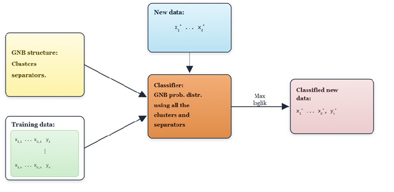
We discuss first the classification in the case when all the features are considered. Based on the training data, we find a GNB structure by applying Algorithm 1. As a result, we obtain a set of clusters and a set of separators that define the GNB structure. With these components as inputs, we describe the main steps involved in the classification process, see Figure 3. Based on the approximation Formula 1 the log-likelihood of a new point $\mathbf{x^{\star}}$ in a class $y\in\{y_{1},\dots,y_{m}\}$ can be calculated.

Input:

The set of clusters and the set of separators which contain the index 0 corresponding the $Y$ target variable: $(0,{i_{k}},{j_{k})\in\mathcal{C}}$ and $(0,{i_{k}})\in\mathcal{S}$ and the corresponding marginal probability distributions: $(Y,X_{i_{k}},X_{j_{k}})$ and $(Y,X_{i_{k}})$ ; A new datapoint $\mathbf{x}=(x^{*}_{1},\dots,x^{*}_{d})$

Log-likelihood evaluation

For each $y_{k}\in\{y_{1},\dots,y_{m}\}$ the log-likelihood of a new datapoints $\mathbf{x^{*}}$ is calculated by using GNB approximation ${p_{GNB}}(y,\mathbf{x^{*}})$ :

	$\displaystyle\log\frac{\prod\limits_{(0,i,j)\in\mathcal{C}}p\left(y_{k},x^{}_{i},x^{}_{j}\right)}{\prod\limits_{(0,s)\in\mathcal{S}}p\left(y_{k},x^{}_{s}\right)^{v_{S}-1}}=\sum\limits_{\left(0,{i},j\right)\in\mathcal{C}}{\log p\left(y_{k},x^{}_{i},x^{*}_{j}\right)}-$
	$\displaystyle-{\sum\limits_{\left(0,s\right)\in\mathcal{S}}{(v_{s}-1)}\log p\left(y_{k},x^{*}_{s}\right)}$

Output:

The class $y_{k}$ with the maximal log-likelihood; Diagnostics: Graph representations on the good and bad classified points projected to the feature pairs selected.

For the Diagnostics see an illustration on the Iris data in F: In Figures 15, 16, 17, one can observe respectively the pairs in the Gaussian case, Gauss copula with KDE marginals, and the most general case where the copula and the marginals are modeled by KDEs.

We emphasize here that we used the default parameters for kernel density estimation, for a general fitting. Although for practitioners interested in a given problem it is worth to finetuning these parameters. Such setting can improve essential the fitting to the training data, see the example in Appendix 18. However this may lead to overfitting on the test data, therefore for finetuning a good idea is to use a validation set.

5.2 Model reduction and classification based on the reduced model

When the number of explanatory attributes is very high, most of the classification methods use feature selection beforehand or regularization in cases like LR and SVM to reduce the number of explanatory variables.

We propose a method that selects one reduced model from a sequence of reduced models. These reduced models are evaluated on the training data. It would also be possible to apply this approach to a validation dataset; however, we chose to rely exclusively on the training data here to ensure comparability with LR and SVM, for which only training data was used.

The reduction procedure has as input the ordered set of clusters obtained from the Structure Learning Algorithm 1.

The smallest reduced model has one cluster. Each new reduced model is obtained from the former one by adding to it a new cluster from the ordered sequence. It is important to point out that by adding greedily new clusters we may obtain a forest as an intermediate structure which is a set of GNB trees, therefore we need to introduce the following concept. The workflow of the method can be seen in Figure .

Definition 22.

We call GNB forest on a set $D^{\prime}\subset D$ a structure which has the property that all of the indices in $D^{\prime}$ are linked to $0$ (which stands for the classification variable $Y$ ) and a forest is defined on the set of indices in $D^{\prime}$ .

Let us denote by $\mathcal{T}_{D^{\prime}}$ the set of disjunct trees defined on $D^{\prime}\subset D$ .

Theorem 23.

The probability distribution corresponding to an intermediate structure constructed from the sequence given by Algorithm 1 is a GNB forest, and the probability distribution assigned is given by

p(Y,\mathbf{X}_{D^{\prime}})=\prod\limits_{T_{k}\in\mathcal{T}}\frac{\prod\limits_{(0,i_{T_{k}},j_{T_{k}})\in\mathcal{C}_{T_{k}}}p(Y,X_{i_{T_{k}}},X_{j_{T_{k}}})}{\prod\limits_{(0,s_{T_{k}})\in\mathcal{S}_{T_{k}}}p(Y,X_{s_{T_{k}}})^{\left(v_{s_{T_{k}}}-1\right)}}\cdot\frac{1}{p(Y)^{{\left|\mathcal{T}\right|}-1}}

(42)

where $\mathcal{T}_{D^{\prime}}$ denotes the forest constructed by Kruskal’s algorithm on the intermediate set of vertices $D^{\prime}$

Proof.

In each step of Algorithm 1 Kruskal’s Algorithm adds a new edge. This can be achieved in two ways: by connecting a new vertex to the existing forest or by adding two new vertices connected by a new edge. In this way in each step a new cluster is added to the GNB forest (Definition 22).

Two clusters (triplets of the form $(0,i,j)$ ) are connected either by only the vertex $0$ or by two vertices one of them is $0$ the other one contained by $D^{\prime}$ , see Figure 4.

When a subset of vertices in $D^{\prime}$ form a tree, the clusters are connected to each other by two vertices (all separators contain two vertices), so this defines sub GNB structure (corresponding to each $T_{k}\in\mathcal{T}$ tree); The probability distribution assigned to a sub-GNB structure corresponding to a $T_{k}\in\mathcal{T}$ tree is

P(\mathbf{X}_{T_{k}})=\frac{\prod\limits_{(0,i_{T_{k}},j_{T_{k}})\in\mathcal{C}_{T_{k}}}p(Y,X_{i_{T_{k}}},X_{j_{T_{k}}})}{{\prod\limits_{(0,s_{T_{k}})\in\mathcal{S}_{T_{k}}}p(Y,X_{s_{T_{k}}})^{\left(v_{s_{T_{k}}}-1\right)}}}

(43)

where $\mathcal{C}_{T_{k}}$ respectively $\mathcal{S}_{T_{k}}$ denotes the set of cluster and separators of the sub-GNB structure.

Let us consider the case when between vertices in $D^{\prime}$ their is no path, i.e. the indices belong to different trees. In this case the GNB forest with the indices of the explanatory variables in $D^{\prime}$ may contain multiple sub-GNB structures, having in common only $Y$ , see Figure 4. The probability distribution assigned is given by the GNB structures involved. The number of the trees is denoted by $\left|\mathcal{T}\right|$ , where $\left|\mathcal{T}\right|\geq 1$ . A GNB structure corresponding to different trees is illustrated in Figure 4. It is easy to see that the intersection between the sub GNB structures is only $Y$ which is an one-element separator. The number of one-element separators of this type are exactly $\left|\mathcal{T}\right|-1$ .

From this observation and Formula 43 it follows immediately the formula of the probability distribution 42 given in the theorem. ∎

Let us note that if we have exactly one tree then $\frac{1}{P(Y)^{\left|\mathcal{T}\right|-1}}$ equals to 1.

The log-likelihood of a sample vector $(\mathbf{x^{*}},y_{k})$ is calculated based on the reduced model 42 restricted to the GNB forest containing the attributes with indices in $D^{\prime}\subset D$ by the following formula:

\begin{array}[]{c}\log p(\mathbf{x^{*}}_{D^{\prime}},y_{k})=\sum\limits_{T_{k}\in\mathcal{T}}\left[\sum\limits_{(0,i_{T_{k}},j_{T_{k}})\in\mathcal{C}_{T_{k}}}\log p(y_{k},x^{*}_{i_{T_{k}}},x^{*}_{j_{T_{k}}})\right.\\ \left.-\sum\limits_{(0,s_{T_{k}})\in\mathcal{S}_{T_{k}}}\left(v_{s_{T_{k}}}-1\right)\log p(y_{k},x^{*}_{s_{T_{k}}})\right]-\left|\mathcal{T}\right|\log p(y_{k})\end{array}

(44)

We assign to the number of clusters/features used by all the reduced models the $f1$ -score calculated on the training data, see the graphs in E. One can chose automatically the number of clusters having the highest average $f1$ -scores over a number of splits (in our experiments this is chosen to be 10). The user can also decide based of the graphics weather a slight improvement is an enough reason to use more clusters. Obviously this function is not a monotonic one.

The selection of the reduce model is illustrated in Figure 5.

The classification procedure based on the reduced model is described as follows:

Input:: The set of indices $D^{\prime}$ ; the GNB forest on $D^{\prime}$ : the set of clusters, set of separators with their multiplicity; the corresponding marginal probability distributions: $(Y,X_{i_{k}},X_{j_{k}})$ and $(Y,X_{i_{k}})$ ; A new datapoint $\mathbf{x}=(x^{*}_{1},\dots,x^{*}_{d})$
Log-likelihood evaluation: For each value of $y=y_{1},\dots,y_{m}$ the log-likelihood of a new datapoint $\mathbf{x^{*}}$ is calculated : $\log p(\mathbf{x^{*}}_{D^{\prime}},y_{k})$ $\blacktriangleright$ Theorem: 44
Output:: The class $y_{k}\in\left\{y_{1},\ldots,y_{m}\right\}$ with the maximal log-likelihood.

6 Numerical Results

The introduced algorithms are designed for the classification task when attributes are continuous, without using discretizations. We will use evaluation metrics specific to this problem: accuracy, precision, recall, $f1$ -score, see D. In the case of more than two classes we used weighted scores. Our algorithms (GNB-Gauss, GNB G-cop, GNB KDE) respectively the reduced models (GNBGauss*, GNB G-cop*, GNB KDE*) were implemented in Python, and will be publicly available for testing.

6.1 Data preparation methods and experiment description

The GNB algorithms introduced in this paper are developed for data characterized by continuous features, without using discretizations. However all data was scaled by min-max scaler, and when two variables correlate more in absolute value than 0.99 we delete one of them. To have a general setting and to be able to apply the algorithms in the same conditions, we choose for all the compared algorithms the same random $15\%$ test set selection, having the same random ten splits (seeds: form 42 to 52).

Relative to our methods we conducted two kinds of experiments. One containing all of the explanatory variables, the second one by using "the best" reduced model. The reduction of the model is made automatically as described in Subsection 5.2 characterizing each of the reduced models by the mean $f1$ score on the training data over the $10$ runs.

In order to compare our algorithms to other glass-box algorithms we run the logistic regression (LR) and Support Vector Machine (SVM) algorithms under different regularization parameter ( $C=1000$ , $C=1$ , $C=0.01$ ) where $C$ stands for regularizing parameter.

6.2 Data description

We give in the following a short description of the datasets in the table 1.

	Num. of	Num. of	Num. of
Dataset	attributes	classes	entries
	(columns)	attributes	(rows)
Abalone [36]	8	3	4180
Body fat [37]	13	3	252
WBCD [38]	30	2	569
Connect [39]	60	2	208
Iris [40]	4	3	150
Wine [41]	14	3	178
Wine quality [42]	12	2	4898

Table 1: Short description of the datasets we used in this paper. The usage of the datasets is described in

In the Diagnostic Wisconsin Breast Cancer Database (WBCD) [38] the aim is to classify a tumor as benign or malignant. The data is slightly unbalanced 0.63 are benign (B) and 0.37 are malign (M). The Abalone data [36] the problem is predicting the sex of abalone shell from physical measurements. The Body fat dataset [37] lists estimates of the percentage of body fat determined by underwater weighing and various body circumference measurements for 252 men. The target variable has three classes. The Iris dataset [40] is a well known dataset with 50 samples from each of the three species. The task is to classify the flowers based on four features. The Connectionist data [39] contains 111 patterns obtained by bouncing sonar signals off a metal cylinder at various angles and under various conditions. Each pattern is a set of 60 numbers in the range 0.0 to 1.0. Each number represents the energy within a particular frequency band, integrated over a certain period of time.The label associated with each record contains the letter "R" if the object is a rock and "M" if it is a mine (metal cylinder).

The Parkinson’s Disease (Parkinson) data set [43] contains biomedical voice measurements. The aim is to discriminate healthy people from those with PD. There are two wine related datasets: Wine data [42] which is related to red variants of the Portuguese "Vinho Verde" wine. The dataset describes the amount of various chemicals present in wine and their effect on it’s quality. The datasets can be viewed as classification task. The classes are ordered and not balanced (e.g. there are much more normal wines than excellent or poor ones). The original task was to predict the quality wine score (0-10) using the given data. This problem was reformulated and the predict good quality wines with score greater or equal than $7$ and average quality wines with their score smaller than $7$ . The second one is Wine quality data [41] which contains results of a chemical analysis of wines grown in the same region in Italy but derived from three different cultivars. The analysis determined the quantities of 13 constituents found in each of the three types of wines.

6.3 Results and discussion

The results are presented in the Tables: 2, 3, 4 and 5. We use for each dataset accuracy, precision, recall and $f1$ scores. When there were more than two classes we used their weighted average, implemented in Python. This way the problems which occur because of unbalanced data can also be observed and compared.

For each of the datasets the tables are presented in two rows. The classification Cases where all features were utilized in the classification are highlighted in yellow. For Logistic regression and SVM we used high value for the inverse of the regularization term $C=1000$ in order to avoid regularization and use all the features. In the white columns, besides Gaussian Naive Bayes (GaussNB), Kernel Naive Bayes (KernelNB) we apply Logistic Regression (LR) and Support Vector Machine (SVM) with different regularization coefficients.

Our newly introduced methods: Gaussian GNB (GNBGauss), Gauss copula with kernel estimated marginals (GNB G-copula) and the most general method where either the joint probability density either the copula an the uni-variate marginals are estimated by kernel densities(GNB KDE). Moreover, we introduced the model reduction possibility in subsection 5.2. The automatically reduced models were denoted by appending a star to their names.

In Table 2, on Abalone dataset: The "all features" winner based on $f1$ score is LR (C=1000) which is also the overall winner; Among the new GNB methods, the highest $f1$ score was achieved by GNB KDE ( $96\%$ of the winner $f1$ score). On Body fat dataset "all feature" winner and overall winner is GNB G-Cop*. Default LR(C=1) and SVM(C=1) are dominated by their version with C=1000 (no regularization). SVM (C=1000) was the closest to the winner ( $99\%$ of the winner $f1$ score).

In Table 3, on WBCD dataset SVM (C=1000) is the "all features" winner, whereas the reduced model winner is LR (C=1); Among our methods The GNB G-cop was the best ( $97.5\%$ of the winner $f1$ score). On Connect dataset GNB KDE model is the "all feature" winner while the reduced GNB KDE* model is the overall best.

In Table 4, on Iris dataset GNB G-cop was "all features" winner, while the reduced model GNB G-cop* also the overall winner; on Parkinson dataset SVM(C=1) is the the overall winner. Among our methods the winner is GNB KDE which achieves ( $95.8\%$ of the winner $f1$ score)

In Table 5, Wine dataset the "all features" and overall winner are the GNBGauss and GNB G-cop methods, among the other methods GaussNB performed also very well. In Wine quality dataset the "all features" and overall winner are the GNB KDE method, among the reduced methods GNB G-cop was the best one. Interestingly to note that LR and SVM methods classified very poorly. On the other hand GaussNB and K.NB performed better than LR and SVM with different parameter setting.

For a good overview, we calculate for each of the datasets the relative $f1$ scores as a fraction obtained by dividing the $f1$ score obtained by each of the methods with the highest $f1$ score achieved on the given dataset (mean over 10 random sampling). Then we calculate the average of these relative $f1$ scores for each of the methods over all of the datasets. The results are presented in Figure 6.

We mention here that in some of the cases the automatic reduced model chores algorithm also decided to use all the explanatory variable. Also it is worth to draw the attention that we use here Gaussian kernels without tuning their parameters, therefore we are sure that for a given problem of interest it is worth to finetuning the parameters in order to get better results. We illustrate this on the Iris data, see Figure 17.

In conclusion, the newly introduced methods are competitive with established glass-box classification methods, such as logistic regression and support vector machines. In many cases, they even outperformed these traditional glass-box approaches. Also important to see that this methods are capable to use as many features as possible by avoiding redundancy since our models exploit the conditional independencies. We highlight here that our reduction method E outputs graphs based on which human decision maker may intervene in the process. These graphs represents how $f1$ score (calculated on the training data) depends on the number of clusters involved on each train test split and the graph obtained by averaging over 10 random splits. Based on these graphs the user may decide on how many clusters to use in the classification task. However in all our experiments this was done automatically, by choosing the number of clusters which achieved the highest $f1$ score on the average of the 10 runs.

Table 2: The table contains the mean accuracy scores (rows) for different methods (columns) over 10 random splits on the Abalone and Body fat test data. We highlighted in yellow when all features were used, and by star our reduced models.

Abalone	GaussNB	K.NB	LR(C=1000)	LR(C=1.0)	LR(C=0,01)	SVM(C=1000)	SVM(C=1)
accuracy	0.5270	0.5118	0.5593	0.5577	0.5308	0.5560	0.5451
precision	0.5127	0.3319	0.5448	0.5443	0.5421	0.5439	0.6938
recall	0.5270	0.5118	0.5593	0.5577	0.5308	0.5560	0.5451
f1-score	0.4783	0.4012	0.5459	0.5420	0.4408	0.5235	0.4475
	SVM(C=0.01)	GNBGauss	GNB G-cop	GNB KDE	GNBGauss*(4/6)	GNB G-cop* (4/6))	GNB KDE*(6/6)
accuracy	0.5278	0.5271	0.5204	0.5376	0.5432	0.5313	0.5376
precision	0.3751	0.5113	0.5015	0.5207	0.5346	0.5133	0.5207
recall	0.5278	0.5271	0.5204	0.5376	0.5432	0.5313	0.5376
f1-score	0.4344	0.5002	0.4982	0.5238	0.5165	0.5077	0.5238
Body fat	GaussNB	K,NB	LR(C=1000)	LR(C=1,0)	LR(C=0,01)	SVM(C=1000)	SVM(C=1)
accuracy	0.6553	0.6289	0.7947	0.7500	0.5789	0.8211	0.7500
precision	0.6811	0.6601	0.7925	0.7683	0.3352	0.8194	0.7697
recall	0.6553	0.6289	0.7947	0.7500	0.5789	0.8211	0.7500
f1-score	0.6576	0.6290	0.7935	0.7273	0.4246	0.8202	0.7240
	SVM(C=0,01)	GNBGauss	GNB G-cop	GNB KDE	GNBGauss*(2/12)	GNB G-cop* (10/12)	GNB KDE* (9/12)
accuracy	0.5789	0.7579	0.8105	0.7579	0.8132	0.8316	0.7868
precision	0.3352	0.7534	0.8096	0.7506	0.8100	0.8302	0.7818
recall	0.5789	0.7579	0.8105	0.7579	0.8132	0.8316	0.7868
f1-score	0.4246	0.7503	0.8068	0.7515	0.8107	0.8280	0.7813

Table 3: The table contains the mean accuracy scores (rows) for different methods (columns) over 10 random splits on the WBCD and Connectionist fat test data. We highlighted in yellow when all features were used, and by star our reduced models.

WBCD	GaussNB	K.NB	LR(C=1000)	LR(C=1.0)	LR(C=0,01)	SVM(C=1000)	SVM(C=1)
accuracy	0.9360	0.9151	0.9663	0.9698	0.7907	0.9651	0.9779
precision	0.9316	0.9881	0.9709	0.9933	1.0000	0.9708	0.9902
recall	0.8938	0.7813	0.9375	0.9250	0.4375	0.9344	0.950000
f1-score	0.9123	0.8726	0.9539	0.9579	0.6087	0.9522	0.9697
	SVM(C=0.01)	GNBGauss	GNB G-cop	GNB KDE	GNBGauss* (29/29)	GNB G-cop* (29/29)	GNB KDE* (28/29)
accuracy	0.8756	0.9570	0.9593	0.9488	0.9570	0.9593	0.9477
precision	1.0000	0.9408	0.9439	0.9423	0.9408	0.9439	0.9421
recall	0.665625	0.9438	0.9469	0.9188	0.9438	0.9469	0.9156
f1-score	0.7993	0.9423	0.9454	0.9304	0.9423	0.9454	0.9287
Connect	GaussNB	K.NB	LR(C=1000)	LR(C=1.0)	LR(C=0,01)	SVM(C=1000)	SVM(C=1)
accuracy	0.6813	0.7000	0.7719	0.7969	0.6906	0.7656	0.7938
precision	0.7656	0.8304	0.7680	0.8000	0.6320	0.7654	0.7889
recall	0.5765	0.5471	0.8176	0.8235	1.0000	0.8059	0.8353
f1-score	0.6577	0.6596	0.7920	0.8116	0.7745	0.7851	0.8114
	SVM(C=0.01)	GNBGauss	GNB G-cop	GNB KDE	GNBGauss* (44/59)	GNB G-cop* (57/59)	GNB KDE* (46/59)
accuracy	0.5313	0.7563	0.8375	0.8563	0.8469	0.8469	0.8656
precision	0.5313	0.8151	0.8172	0.8407	0.8805	0.8235	0.8470
recall	1.0000	0.7000	0.8941	0.9000	0.8235	0.9059	0.9118
f1-score	0.6939	0.7532	0.8539	0.8693	0.8511	0.8627	0.8782

Table 4: The table contains the mean accuracy scores (rows) for different methods (columns) over the same 10 random splits on the Iris and Parkinson data. We highlighted in yellow when all features were used, and by star our reduced models.

Iris	GaussNB	K.NB	LR(C=1000)	LR(C=1.0)	LR(C=0,01)	SVM(C=1000)	SVM(C=1)
accuracy	0.9565	0.9087	0.9870	0.9261	0.7391	0.9783	0.9565
precision	0.9567	0.9137	0.9870	0.9272	0.8217	0.9783	0.9567
recall	0.9565	0.9087	0.9870	0.9261	0.7391	0.9783	0.9565
f1-score	0.9565	0.9082	0.9870	0.9260	0.6825	0.9783	0.9565
	SVM(C=0.01)	GNBGauss	GNB G-cop	GNB KDE	GNBGauss* (2/4)	GNB G-cop* (3/4)	GNB KDE* (2/4)
accuracy	0.3043	0.9826	0.9913	0.9826	0.9870	0.9913	0.9826
precision	0.3043	0.9828	0.9913	0.9828	0.9870	0.9913	0.9828
recall	0.3043	0.9826	0.9913	0.9826	0.9870	0.9913	0.9826
f1-score	0.2806	0.9826	0.9913	0.9826	0.9870	0.9913	0.9826
Parkinson	GaussNB	K.NB	LR(C=1000)	LR(C=1.0)	LR(C=0,01)	SVM(C=1000)	SVM(C=1)
accuracy	0.7267	0.7833	0.8500	0.8600	0.7667	0.8267	0.8700
precision	0.8230	0.8702	0.8455	0.8610	0.5878	0.8193	0.8838
recall	0.7267	0.7833	0.8500	0.8600	0.7667	0.8267	0.8700
f1-score	0.7472	0.7994	0.8472	0.8438	0.6654	0.8218	0.8515
	SVM(C=0.01)	GNBGauss	GNB G-cop	GNB KDE	GNBGauss* (14/15)	GNB G-cop*	GNB KDE*(15/15)
accuracy	0.7667	0.7067	0.8067	0.8067	0.7000	0.8067	0.8067
precision	0.5878	0.7886	0.8195	0.8350	0.7861	0.8048	0.8350
recall	0.7667	0.7067	0.8067	0.8067	0.7000	0.8067	0.8067
f1-score	0.6654	0.7277	0.8117	0.8155	0.7218	0.8057	0.8155

Table 5: The table contains the mean accuracy scores (rows) for different methods (columns) over the same 10 random splits on the Wine and Wine quality data. We highlighted in yellow when all features were used, and by star our reduced models.

Wine	GaussNB	K.NB	LR(C=1000)	LR(C=1.0)	LR(C=0,01)	SVM(C=1000)	SVM(C=1)
accuracy	0.9926	0.9222	0.9741	0.9778	0.5630	0.9667	0.9778
precision	0.9928	0.9318	0.9740	0.9786	0.5299	0.9672	0.9795
recall	0.9926	0.9222	0.9741	0.9778	0.5630	0.9667	0.9778
f1-score	0.9926	0.9207	0.9740	0.9777	0.4773	0.9666	0.9779
	SVM(C=0.01)	GNBGauss	GNB G-cop	GNB KDE	GNBGauss* (12/12)	GNB G-cop* (12/12)	GNB KDE* (12/12)
accuracy	0.4074	1.0000	1.0000	0.9889	1.0000	1.0000	0.9889
precision	0.1660	1.0000	1.0000	0.9893	1.0000	1.0000	0.9893
recall	0.4074	1.0000	1.0000	0.9889	1.0000	1.0000	0.9889
f1-score	0.2359	1.0000	1.0000	0.9889	1.0000	1.0000	0.9889
Wine quality	GaussNB	K.NB	LR(C=1000)	LR(C=1.0)	LR(C=0,01)	SVM(C=1000)	SVM(C=1)
accuracy	0.7443	0.6788	0.8185	0.8204	0.8031	0.8031	0.8031
precision	0.4040	0.3583	0.5884	0.6234	0.0000	0.0000	0.0000
recall	0.6281	0.7984	0.2599	0.2224	0.0000	0.0000	0.0000
f1-score	0.4917	0.4947	0.3605	0.3278	0.0000	0.0000	0.0000
	SVM(C=0.01)	GNBGauss	GNB G-cop	GNB KDE	GNBGauss* (12/12)	GNB G-cop* (10/10)	GNB KDE* (12/12)
accuracy	0.8031	0.7753	0.8009	0.8181	0.7753	0.8009	0.8181
precision	0.0000	0.4502	0.4942	0.5369	0.4502	0.4942	0.5369
recall	0.0000	0.6375	0.4688	0.5526	0.6375	0.4688	0.5526
f1-score	0.0000	0.5277	0.4812	0.5447	0.5277	0.4812	0.5447

7 Conclusion

This paper discusses the classification based on fitting GNB structures to data when the explanatory variables are continuous. We introduce the theoretical background to solve this problem under different assumption on the joint probability distribution between the explanatory variables: joint a Gaussian distribution; the more general case when the uni-variate marginals may have various distributions, and the dependence is characterized by a Gaussian copula; and an even more general case when we have no restriction on the joint density (copula or marginals). We proved, that the KL divergence depends on the GNB structure only through the pair copulas associated to the bi-variate marginals. We give under each of the assumptions a classification method. Moreover we give also a feature/cluster reduction methodology together with a classification based on the concept of GNB forest. The GNB structure learning based on data was also discussed from combinatorial point of view. We proved that the GNB structures may be assigned to the basis of a matroid. This ensures the existence of a greedy algorithm with an optimality guarantee, in the sense of minimizing the KL divergence. For finding such greedy algorithm we defined a weighted complete graph on the set of indices, and proved that applying to it the Kruskal’s algorithm we obtain the optimal GNB structure. We introduced a more general structure allowing more complex dependence structure between the attributes ( $k\geq 3$ interconnected features) called $k$ -GNB models, and discussed from mathematical point of view the Gaussian case. For $k\geq 3$ there are no guarantees for finding the optimal structure even for the Gaussian case.

Advantages: A significant strength of the new algorithms, in contrast to black-box algorithms, is their explainability. Therefore the GNB structures can be considered an interpretable machine learning tool. A huge advantage of using the simple GNB approach is that all marginal probability distributions used for classification are of order 3. Even in the more general cases, when $k>3$ it is an advantage to chose small values for $k$ ; Low dimensional marginals can be more trustfully approximated from data, even if the data is not very large. Therefore, our algorithms also work well in cases with many features and relatively small datasets. We observed that via model reduction the accuracy of the classification is typically improved. The output graphs are usable for experts in deciding on how many clusters should be considered. This way, they may intervene in the classification loop. All the proposed algorithms for GNB were tested and compared under the same conditions. It turned out that our algorithms are competitive, in many cases even better than the popular Glass-box models. Our algorithms were implemented in Python, a demo repository can be found at
https://github.com/AbrahamPapp/generalized-naive-bayes-demo. We will publish also the package developed by the first author.

Limitations: The Gaussian classification method should be used with precaution. The copula based methods need in the classification task the kernel densities fitted to the training data. Using the default parameters may be suboptimal. We recommend fine-tuning the parameters involved with respect to the given problem. Another drawback may occur even in the cases when we have nice guarantee on the optimality of structure on the training data, this gives no guarantee on its efficiency on the test data. However the method of reduction may overcome this issue.

Future work: We plan to accelerate the algorithm and discuss it for higher values of $k\geq 3$ . Additionally, we intend to release a Python package containing these algorithms.

We anticipate that this work will be advantageous for classification problems in fields where acquiring large sample data is very expensive or time-consuming.

Acknowledgements

The research reported in this paper was partially supported by project no. BME-NVA-02, implemented with the support provided by the Ministry of Innovation and Technology of Hungary from the National Research, Development and Innovation Fund, financed under the TKP2021 funding scheme.

References

[1] H. Zhang, L. Jiang, L. Yu, Attribute and instance weighted naive Bayes, Pattern Recognition 111 (2021).
[2] X. Wu, V. Kumar, J. Ross Quinlan, J. Ghosh, Q. Yang, H. Motoda, G. J. McLachlan, A. Ng, B. Liu, P. S. Yu, et al., Top 10 algorithms in data mining, Knowledge and information systems 14 (1) (2008) 1–37.
[3] D. Petschke, T. E. Staab, A supervised machine learning approach using naive gaussian bayes classification for shape-sensitive detector pulse discrimination in positron annihilation lifetime spectroscopy (pals), Nuclear Instruments and Methods in Physics Research Section A: Accelerators, Spectrometers, Detectors and Associated Equipment 947 (2019) 162742.
[4] J. S. Aguilar-Ruiz, C. Romero-Vargas, Xnb: A package for class-specific naive-bayes classifier, SoftwareX 32 (2025) 102347.
[5] G.-L. Ou, Y.-L. He, P. Fournier-Viger, J. Z. Huang, A novel multi-source weighted naive bayes classifier, Information Sciences (2025) 122568.
[6] J. G. Brandao, A. P. C. Junior, V. M. G. Pacheco, C. G. Rodrigues, O. M. O. Belo, A. P. Coimbra, W. P. Calixto, Optimization of machine learning models for sentiment analysis in social media, Information Sciences 694 (2025) 121704.
[7] P. Torrijos, J. C. Alfaro, J. A. Gámez, J. M. Puerta, Federated learning with discriminative naive bayes classifier, in: International Conference on Intelligent Data Engineering and Automated Learning, Springer, 2024, pp. 328–339.
[8] N. Friedman, M. Goldszmidt, T. J. Lee, Bayesian network classification with continuous attributes: Getting the best of both discretization and parametric fitting., in: ICML, Vol. 98, 1998, pp. 179–187.
[9] N. Friedman, D. Geiger, M. Goldszmidt, Bayesian network classifiers, Machine learning 29 (1997) 131–163.
[10] A. Perez, P. Larranaga, I. Inza, Supervised classification with conditional gaussian networks: Increasing the structure complexity from naive bayes, International Journal of Approximate Reasoning 43 (1) (2006) 1–25.
[11] M. Sahami, Learning limited dependence bayesian classifiers., in: KDD, Vol. 96, 1996, pp. 335–338.
[12] A. Pérez, P. Larrañaga, I. Inza, Bayesian classifiers based on kernel density estimation: Flexible classifiers, International Journal of Approximate Reasoning 50 (2) (2009) 341–362.
[13] S. Chen, G. I. Webb, L. Liu, X. Ma, A novel selective naïve Bayes algorithm, Knowledge-Based Systems 192 (2020).
[14] R. Blanquero, E. Carrizosa, P. Ramírez-Cobo, M. R. Sillero-Denamiel, Variable selection for naïve bayes classification, Computers & Operations Research 135 (2021) 105456.
[15] L. Wang, X. Zhang, K. Li, S. Zhang, Semi-supervised learning for k-dependence bayesian classifiers, Applied Intelligence 52 (4) (2022) 3604–3622.
[16] L. Wang, L. Li, Q. Li, K. Li, Learning high-dependence bayesian network classifier with robust topology, Expert Systems with Applications 239 (2024) 122395.
[17] K. Meng, H. Zhang, L. Jiang, P. Lv, S. He, M. Xu, K-free dependence bayesian classifiers, IEEE Transactions on Neural Networks and Learning Systems (2026).
[18] W. Wang, L. Yan, F. Liu, Y. Li, Improving gaussian naive bayes classification on imbalanced data through coordinate-based minority feature mining, PeerJ Computer Science 11 (2025) e3003.
[19] G.-L. Ou, Y.-L. He, Y.-C. Cheng, J. Z. Huang, Relaxed naïve bayesian classifier based on maximum dependent attribute groups, Information Sciences 707 (2025) 122013.
[20] Y. Ren, L. Wang, X. Li, M. Pang, J. Wei, Stochastic optimization for bayesian network classifiers, Applied Intelligence 52 (13) (2022) 15496–15516.
[21] R. R. Bouckaert, Naive bayes classifiers that perform well with continuous variables, in: Australasian joint conference on artificial intelligence, Springer, 2004, pp. 1089–1094.
[22] A. Ng, M. Jordan, On discriminative vs. generative classifiers: A comparison of logistic regression and naive bayes, Advances in neural information processing systems 14 (2001).
[23] J.-H. Xue, D. M. Titterington, Comment on “on discriminative vs. generative classifiers: A comparison of logistic regression and naive bayes”, Neural processing letters 28 (3) (2008) 169–187.
[24] E. A. Kovács, A. Ország, D. Pfeifer, A. Benczúr, Generalized naive bayes, Pattern Recognition (2025) 112927.
[25] D. M. Chickering, Learning bayesian networks is np-complete, in: Learning from data: Artificial intelligence and statistics V, Springer, 1996, pp. 121–130.
[26] E. Kovács, T. Szántai, On the approximation of a discrete multivariate probability distribution using the new concept of t-cherry junction tree, in: Coping with Uncertainty, Springer, 2010, pp. 39–56.
[27] T. Szántai, E. Kovács, Hypergraphs as a mean of discovering the dependence structure of a discrete multivariate probability distribution, Annals of Operations Research 193 (1) (2012) 71–90.
[28] M. Sklar, Fonctions de répartition à n dimensions et leurs marges, in: Annales de l’ISUP, Vol. 8, 1959, pp. 229–231.
[29] A. Sklar, Random variables, distribution functions, and copulas: a personal look backward and forward, Lecture notes-monograph series (1996) 1–14.
[30] T. M. Cover, J. A. Thomas, Elements of information theory, John Wiley & Sons, 2012.
[31] S. Kullback, R. A. Leibler, On information and sufficiency, The annals of mathematical statistics 22 (1) (1951) 79–86.
[32] J. Ma, Z. Sun, Mutual information is copula entropy, Tsinghua Science & Technology 16 (1) (2011) 51–54.
[33] R. B. Nelsen, An introduction to copulas, Springer, 2006.
[34] H. Whitney, On the abstract properties of linear dependence, in: Hassler Whitney Collected Papers, Springer, 1992, pp. 147–171.
[35] F. Ghofrani, A. Keshavarz-Haddad, A. Jamshidi, A new probabilistic classifier based on decomposable models with application to internet traffic, Pattern Recognition 77 (2018) 1–11.
[36] S. T. T. S. C. A. Nash, Warwick, W. Ford, Abalone, UCI Machine Learning Repository, DOI: https://doi.org/10.24432/C55C7W (1994).
[37] K. W. Penrose, A. G. Nelson, A. G. Fisher, Generalized body composition prediction equation for men using simple measurement techniques, Medicine & Science in Sports & Exercise 17 (2) (1985) 189.
[38] https://archive.ics.uci.edu/dataset/17/breast+cancer+wisconsin+diagnostic.
[39] T. Sejnowski, R. Gorman, Connectionist Bench (Sonar, Mines vs. Rocks), UCI Machine Learning Repository, DOI: https://doi.org/10.24432/C5T01Q (1988).
[40] R. A. Fisher, Iris, UCI Machine Learning Repository, DOI: https://doi.org/10.24432/C56C76 (1936).
[41] S. Aeberhard, M. Forina, Wine, UCI Machine Learning Repository, DOI: https://doi.org/10.24432/C5PC7J (1992).
[42] C. A. A. F. M. T. Cortez, Paulo, J. Reis, Wine Quality, UCI Machine Learning Repository, DOI: https://doi.org/10.24432/C56S3T (2009).
[43] https://www.kaggle.com/datasets/thecansin/parkinsons-data-set.

Appendix A cherry junction tree of order $k$

We call the structure assigned to a cherry tree graph of order $k$ a cherry-junction tree of order k, and define it as follows:

1.

The set of vertices in each $k$ th order maximum clique is called a cluster, and contains its $k$ vertices.
2.
Two $k$ -element clusters are connected if the following two conditions are fulfilled:
- •
  
  the clusters share $k-1$ elements
- •
  
  if a set of $k-1$ elements is contained by $m$ clusters, these clusters will be connected tree-like by $m-1$ edges.
3.

The $k-1$ -element set given by the intersection of two connected clusters is called a separator. The number of clusters containing it is the multiplicity of the separator.

A cherry-junction tree is characterized by the set of indices $V$ , the set of clusters $\mathcal{C}$ , the set of separators $\mathcal{S}$ and a dictionary of the multiplicities of the separators $\mathcal{M}$ .

The associated probability distribution has the formula:

p_{GNB}(\mathbf{x})=\frac{\prod\limits_{C\in\mathcal{C}}p\left(\mathbf{x}_{C}\right)}{\prod\limits_{S\in\mathcal{S}}p\left(\mathbf{x}_{S}\right)^{v_{S}-1}}

Appendix B Information content of continuous and discrete random vector

Proof.

The entropy of the random vector $(\mathbf{X},Y)=(X_{1},...,X_{d},Y)$ is the following:

H(\mathbf{X},Y)=-\sum\limits_{y_{k}\in\mathcal{Y}}\int_{\mathbf{\chi}}p(\mathbf{x},y_{k})\log p(\mathbf{x},y_{k})dx

We express $p(\mathbf{x},y)$ from the conditional probability distribution formula:

p(\mathbf{x}|Y)=\frac{p(\mathbf{x},y)}{p(Y)}\implies p(\mathbf{x},y)=p(Y)p(\mathbf{x}|Y)

and substitute it in the formula of the joint entropy:

$\displaystyle H(\mathbf{X},Y)$	$\displaystyle=$	$\displaystyle-\sum\limits_{y_{k}\in\mathcal{Y}}\int_{\mathbf{\chi}}p(y_{k})p(\mathbf{x}\|y_{k})\log[p(y_{k})p(\mathbf{x}\|y_{k})]dx=$
	$\displaystyle=$	$\displaystyle-\sum\limits_{y_{k}\in\mathcal{Y}}p(y_{k})\int_{\mathbf{\chi}}p(\mathbf{x}\|y_{k})\log[p(y_{k})p(\mathbf{x}\|y_{k})]dx=$
	$\displaystyle=$	$\displaystyle-\sum\limits_{y_{k}\in\mathcal{Y}}\left[p(y_{k})\int_{\mathbf{\chi}}p(\mathbf{x}\|y_{k})\log p(y_{k})+p(\mathbf{x}\|y_{k})\log p(\mathbf{x}\|y_{k})\right]dx=$
	$\displaystyle=$	$\displaystyle-\sum\limits_{y_{k}\in\mathcal{Y}}\left(p(y_{k})\log p(y_{k})\underset{1}{\underbrace{\int_{\mathbf{\chi}}p(\mathbf{x}\|y_{k})dx}}+p(y_{k})\int_{\mathbf{\chi}}p(\mathbf{x}\|y_{k})\log p(\mathbf{x}\|y_{k})dx\right)=$
	$\displaystyle=$	$\displaystyle-\sum\limits_{y_{k}\in\mathcal{Y}}p(y_{k})\log p(y_{k})+\sum\limits_{y_{k}\in\mathcal{Y}}p(y_{k})H(\mathbf{X}\|y_{k})=$
	$\displaystyle=$	$\displaystyle H(Y)+\sum\limits_{y_{k}\in\mathcal{Y}}p(y_{k})H(\mathbf{X}\|y_{k})$

By using the formula of joint entropy, we can express the formula of information content as follows:

$\displaystyle I(\mathbf{X},Y)$	$\displaystyle=$	$\displaystyle\sum\limits_{i=1}^{d}H(X_{i})+H(Y)-H(\mathbf{X},Y)=$
	$\displaystyle=$	$\displaystyle\sum\limits_{i=1}^{d}H(X_{i})+H(Y)-\left(H(Y)+\sum\limits_{y_{k}\in\mathcal{Y}}p(y_{k})H(\mathbf{X}\|y_{k})\right)$
	$\displaystyle=$	$\displaystyle\sum\limits_{i=1}^{d}H(X_{i})-\sum\limits_{y_{k}\in\mathcal{Y}}p(y_{k})H(\mathbf{X}\|y_{k})$

∎

Appendix C Mutual information Gauss and discrete random variables

$\displaystyle I(X,Y)$	$\displaystyle=$	$\displaystyle H(X)-\sum\limits_{y_{k}\in\mathcal{Y}}p(y_{k})H(X\|y_{k})=$	(45)
	$\displaystyle=$	$\displaystyle\frac{1}{2}\log(2\pi e\sigma_{X}^{2})-\sum\limits_{y_{k}\in\mathcal{Y}}p(y_{k})\left[\frac{1}{2}\log(2\pi e\sigma_{X\|y_{k}}^{2})\right]=$
	$\displaystyle=$	$\displaystyle\frac{1}{2}\left(\log 2\pi+1+\log\sigma_{X}^{2}\right)+\frac{-1}{2}\sum\limits_{y_{k}\in\mathcal{Y}}p(y_{k})\left[\log(2\pi)+1+\log\sigma_{X\|y_{k}}^{2}\right]=$
	$\displaystyle=$	$\displaystyle\frac{1}{2}\left[\left(\log 2\pi+1+\log\sigma_{X}^{2}\right)-\log(2\pi)-1-\sum\limits_{y_{k}\in\mathcal{Y}}p(y_{k})\log\sigma_{X\|y_{k}}^{2}\right]=$
	$\displaystyle=$	$\displaystyle\frac{1}{2}\left(\log\sigma^{2}_{X}-\sum\limits_{y_{k}\in\mathcal{Y}}p(y_{k})\log\sigma^{2}_{X\|y_{k}}\right)$

Appendix D Evaluation metrics

In binary classification, beyond accuracy, precision and recall are often used metrics to evaluate the models. Let the labels we want to predict be ‘positive’ and ‘negative’, then we can define the confusion matrix, in which the columns show the actual values and the rows show the predicted values:

		Actual
		Positive	Negative
Predicted	Positive	#{True Positive}	#{False Positive}
Predicted	Negative	#{False Negative}	#{True Negative}

There are four possible outcomes according to the actual and the predicted label. The elements of the matrix show the occurrence of each outcome. Based on these accuracy, precision and recall can be defined as follows:

\textrm{Accuracy}=\frac{\#\{\textrm{True Positive}\}+\#\{\textrm{True Negative}\}}{\#\{Total\}}

\textrm{Precision}=\frac{\#\{\textrm{True Positive}\}}{\#\{\textrm{True Positive}\}+\#\{\textrm{False Positive}\}}

\textrm{Recall}=\frac{\#\{\textrm{True Positive}\}}{\#\{\textrm{True Positive}\}+\#\{\textrm{False Negative}\}}

\textrm{f1 score}=2\times\frac{\textrm{Precision}\times\textrm{Recall}}{\textrm{Precision}+\textrm{Recall}}

Appendix E Model reduction based on graphs

Appendix F Pair diagnostic graphs

Illustration of the diagnostics for the Iris Data for the feature pairs used in the GNB structure under different assumptions/methods applied.

	$\displaystyle\log\|K_{X_{l}X_{m}\|y_{i}}\|$	$\displaystyle=$	$\displaystyle\log\left[\sigma_{l\|y_{i}}^{2}\sigma_{m\|y_{i}}^{2}(1-\rho^{2}_{lm\|y_{i}})\right]$
		$\displaystyle=$	$\displaystyle\log\sigma_{l\|y_{i}}^{2}+\log\sigma_{m\|y_{i}}^{2}+\log(1-\rho^{2}_{lm\|y_{i}})$

$\displaystyle W$	$\displaystyle=$	$\displaystyle\frac{1}{2}\sum\limits_{C\in\mathcal{C}}\left[\sum\limits_{i\in C}\log\sigma_{X_{i}}^{2}-\sum\limits_{y_{k}\in\mathcal{Y}}p\left(y_{k}\right)\log\left\|K_{X_{C}\|y_{k}}\right\|\right]-$
		$\displaystyle-\frac{1}{2}\sum\limits_{S\in\mathcal{S}}\left(\nu_{S}-1\right)\left[\sum\limits_{i\in S}\log\sigma_{X_{i}}^{2}-\sum\limits_{y_{k}\in\mathcal{Y}}p\left(y_{k}\right)\log\left\|K_{X_{S\|y_{k}}}\right\|\right]$
	$\displaystyle=$	$\displaystyle\frac{1}{2}\sum\limits_{i=1}^{D}\log\sigma_{X_{i}}^{2}-\frac{1}{2}\left[\sum\limits_{C\in\mathcal{C}}\sum\limits_{y_{k}\in\mathcal{Y}}p\left(y_{k}\right)\log\left\|K_{X_{C}}\right\|\right.$
		$\displaystyle\left.-\sum\limits_{S\in\mathcal{S}}\left(\nu_{S}-1\right)\sum\limits_{y_{k}\in\mathcal{Y}}p\left(y_{k}\right)\log\left\|K_{X_{S\|y_{k}}}\right\|\right]$

On Generalized Naive Bayes with Continuous Features

Abstract

Keywords:

MSC

1 Introduction

2 Preliminaries

2.1 The GNB structures

Definition 1.

2.2 Results related to copula theory

Definition 2.

Theorem 3.

2.3 Information theoretical concepts

Theorem 4.

Definition 5.

Theorem 6.

3 The weight of a GNB approximation under different assumptions on the joint distribution of the explanatory variables

3.1 Features following joint Gaussian distribution

Theorem 7.

Proof.

Remark 8.

3.2 GNB with a general nonparametric joint continuous distribution between the explanatory variables

Lemma 9.

Proof.

Remark 10.

Theorem 11.

Proof.

Remark 12.

Remark 13.

3.3 Joint dependence structure characterized by Gauss copula

Theorem 14.

Proof.

Remark 15.

4 Combinatorial background of the GNB and greedy structure learning algorithms

4.1 Mathematical structure

Definition 16.

Theorem 17.

Proof.

Theorem 18.

Proof.

Remark 19.

4.2 Greedy algorithms for structure learning

4.3 Discussion on higher order dependencies between the attributes

Definition 20.

Theorem 21.

Proof.

5 The classification procedure and model reduction

5.1 All features classification procedure

5.2 Model reduction and classification based on the reduced model

Definition 22.

Theorem 23.

Proof.

6 Numerical Results

6.1 Data preparation methods and experiment description

6.2 Data description

6.3 Results and discussion

7 Conclusion

Acknowledgements

References

Appendix A cherry junction tree of order kk

Appendix B Information content of continuous and discrete random vector

Proof.

Appendix C Mutual information Gauss and discrete random variables

Appendix D Evaluation metrics

Appendix E Model reduction based on graphs

Appendix F Pair diagnostic graphs

Appendix A cherry junction tree of order $k$